extrapolation for time-series and cross-sectional data … · · 2017-01-26extrapolation for...

Principles of Forecasting: A Handbook for Researchers and Practitioners, J. Scott Armstrong (ed.): Norwell, MA: Kluwer Academic Publishers, 2001

May 18, 2000

Extrapolation for Time-Series

and Cross-Sectional Data

J. Scott Armstrong The Wharton School, University of Pennsylvania

ABSTRACT

Extrapolation methods are reliable, objective, inexpensive, quick, and easily automated. As a result, they are widely used, especially for inventory and production forecasts, for operational planning for up to two years ahead, and for long-term forecasts in some situations, such as population forecasting. This paper provides principles for selecting and preparing data, making seasonal adjustments, extrapolating, assessing uncertainty, and identifying when to use extrapolation. The principles are based on received wisdom (i.e., experts’ commonly held opinions) and on empirical studies. Some of the more important principles are:

• In selecting and preparing data, use all relevant data and adjust the data for important events that occurred in the past.

• Make seasonal adjustments only when seasonal effects are expected and only if there is

good evidence by which to measure them.

• In extrapolating, use simple functional forms. Weight the most recent data heavily if there are small measurement errors, stable series, and short forecast horizons. Domain knowledge and forecasting expertise can help to select effective extrapolation procedures. When there is uncertainty, be conservative in forecasting trends. Update extrapolation models as new data are received.

• To assess uncertainty, make empirical estimates to establish prediction intervals.

• Use pure extrapolation when many forecasts are required, little is known about the situation,

the situation is stable, and expert forecasts might be biased.

Key words: acceleration, adaptive parameters, analogous data, asymmetric errors, base rate, Box-Jenkins, combining, conservatism, contrary series, cycles, damping, decomposition, discontinuities, domain knowledge, experimentation, exponential smoothing, functional form, judgmental adjustments, M-competition, measurement error, moving averages, nowcasting, prediction intervals, projections, random walk, seasonality, simplicity, tracking signals, trends, uncertainty, updating.

EXTRAPOLATION 2

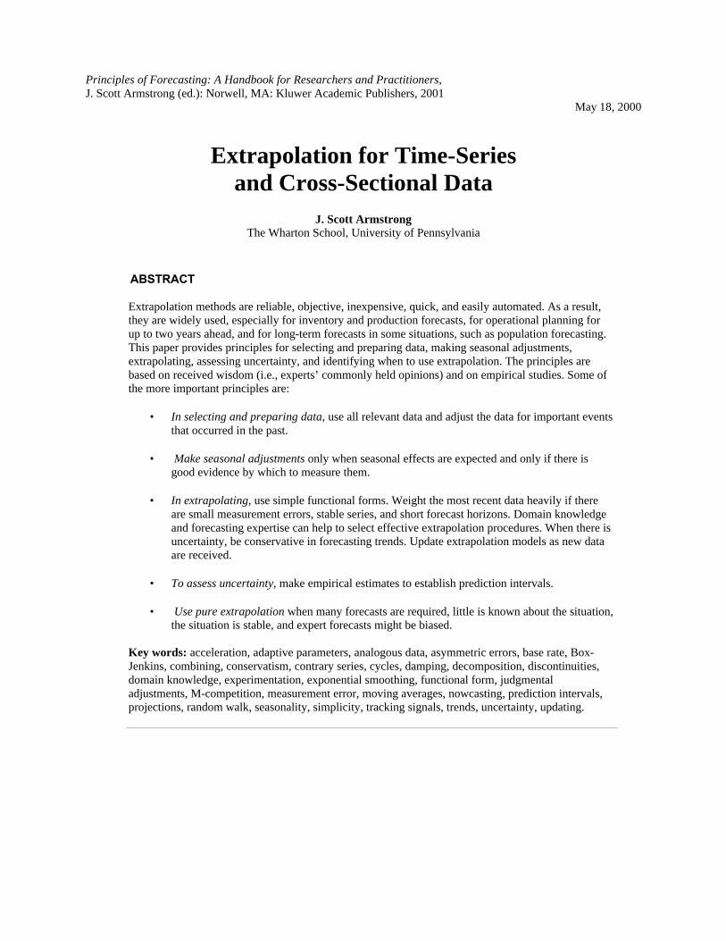
Time-series extrapolation, also called univariate time-series forecasting or projection, relies on quantitative methods to analyze data for the variable of interest. Pure extrapolation is based only on values of the variable being forecast. The basic assumption is that the variable will continue in the future as it has behaved in the past. Thus, an extrapolation for Exhibit 1 would go up.

Exhibit 1A Time Series

1.60

0.00

0.20

0.40

0.60

0.80

1.00

1.20

1.40

1965

1970

1975

1980

1985

1990

1995

Extrapolation can also be used for cross-sectional data. The assumption is that the behavior of some actors at a given time can be used to extrapolate the behavior of others. The analyst should find base rates for similar populations. For example, to predict whether a particular job applicant will last more than a year on the job, one could use the percentage of the last 50 people hired for that type of job who lasted more than a year. Academics flock to do research on extrapolation. It is a statistician’s delight. In early 2000, using a search for the term time series (in the title or key words), I found listings in the Social Science Citation Index (SSCI) for over 5,600 papers published in journals since 1988; adding the term forecasting reduced this to 580 papers. I found 730 by searching on seasonality, decreased to 41 when the term forecasting was added. Searching for extrapolation yielded 314 papers, reduced to 43 when forecasting was added. Little of this research has contributed to the development of forecasting principles. In my paper, only 16 studies published during this period seemed relevant to the development of principles for extrapolation. Few statisticians conduct studies that allow one to generalize about the effectiveness of their methods. When other researchers test the value of their procedures, they show little interest and seldom cite findings about the accuracy of their methods. For example, Fildes and Makridakis (1995) checked the SSCI and SCI (Science Citation Index) to determine the number of times researchers cited four major comparative validation studies on time series forecasting (Newbold and Granger 1974; Makridakis and Hibon 1979; Meese and Geweke 1984; and Makridakis et al. 1982). Between 1974 and 1991, a period in which many thousands of time-series studies were published, these four comparative studies were cited only three times per year in all the statistics journals indexed. In short, they were virtually ignored by statisticians. I found some research to be useful, especially studies comparing alternative extrapolation methods on common data sets. Such studies can contribute to principles for extrapolation when they contain descriptions of the conditions. In reviewing the literature, I looked at references in key papers. In addition, using the term “extrapolation,” I searched the SSCI for papers published from 1988 to 2000. I sent drafts of my paper to key researchers and practitioners, asking them what papers and principles might have been overlooked. I also posted the references and principles on the Forecasting Principles website, hops.wharton.upenn.edu/forecast, in August 1999, and issued a call to various e-mail lists for information about references that should be included.

PRINCIPLES OF FORECASTING

3

The first part of the paper describes the selection and preparation of data for extrapolation, the second considers seasonal adjustments, the third examines making extrapolations, and the fourth discusses the assessment of uncertainty. The paper concludes with principles concerning when to use extrapolation SELECTING AND PREPARING DATA Although extrapolation requires only data on the series of interest, there is also a need for judgment, particularly in selecting and preparing the data.

• Obtain data that represent the forecast situation.

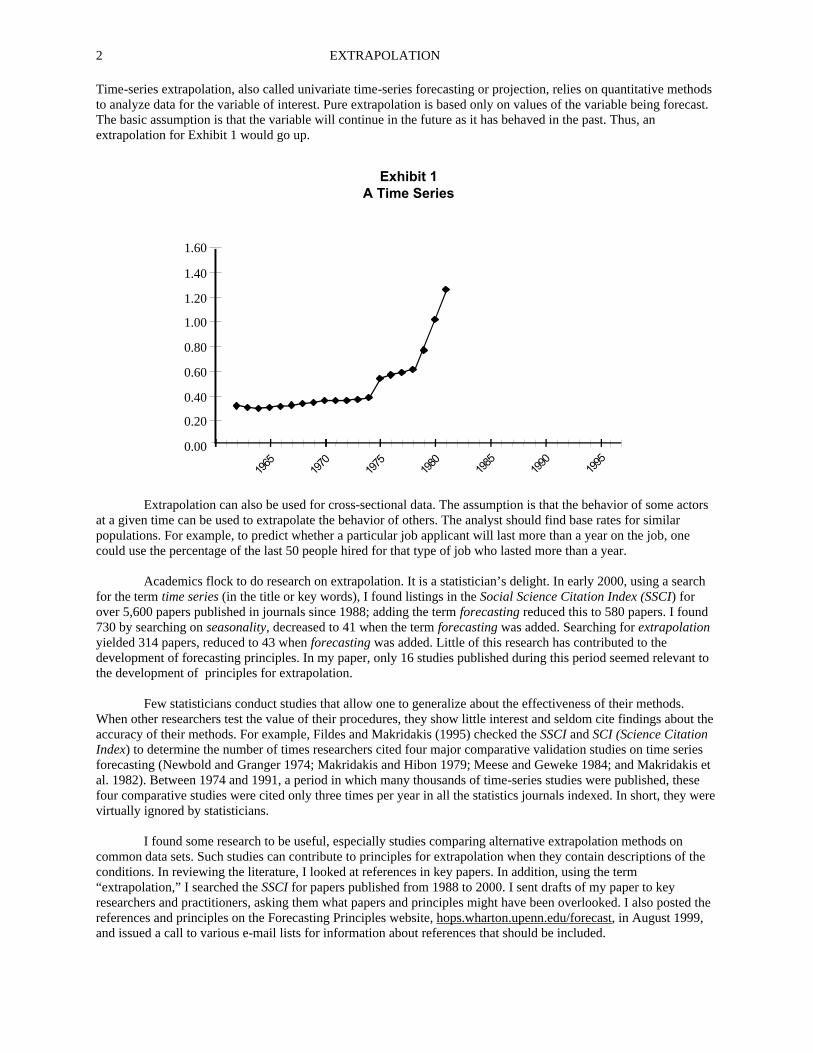
For extrapolation, you need data that represent the events to be forecast. Rather than starting with data, you should ask what data the problem calls for. For example, if the task calls for a long-term forecast of U.S. retail prices of gasoline, you need data on the average pump prices in current dollars. Exhibit 1 presents these data from 1962 through 1981. The gasoline case is typical of many situations in which ample data exist on the variable to be forecast. Sometimes it is not obvious how to measure the variable of interest. For example, if you want to extrapolate the number of poor people in the U.S., you must first define what it means mean to be poor. Alternate measures yield different estimates. Those who use income as the measure conclude that the number of poor is increasing, while those who use the consumption of goods and services conclude that the number is decreasing. If you have few data on the situation, you should seek data from analogous situations. For example, to forecast the start-up pattern of sales at a new McDonald’s franchise, you could extrapolate historical data from McDonald’s start-ups in similar locations. If you can find no similar situations, you can develop laboratory or field experiments. Experiments are especially useful for assessing the effects of large changes. Marketers have used laboratory experiments for many years, for example, in testing new products in simulated stores. Nevin (1974) tested the predictive validity of consumer laboratory experiments, finding that they provided good estimates of market share and market share for some brands. Analysts have used laboratory simulations successfully to predict personnel behavior by using work samples (Reilly and Chao 1982, Robertson and Kandola 1982, and Smith 1976). In these simulations, subjects are asked to perform typical job duties. From their performance on sample tasks, analysts extrapolated their behavior on the job. For greater realism, analysts may conduct field experiments. Compared to lab experiments, field experiments are costly, offer less control over key factors, and have little secrecy. Field experiments are used in many areas, such as marketing, social psychology, medicine, and agriculture. The validity of the extrapolation depends upon how closely the experiment corresponds to the given situation. For example, when running field experiments in a test market for a new product, you must first generalize from the sample observations to the entire test market, then from the test market to the total market, and finally to the future. In addition, such experiments can be influenced by researchers’ biases and by competitors’ actions. Exhibit 2 summarizes different types of data sources. I rated them against five criteria. No one source provides the best data for all situations. When large structural changes are expected, traditional extrapolation of historical data is less appropriate than extrapolations based on analogous data, laboratory simulations, or field experiments.

EXTRAPOLATION 4

Exhibit 2: Ranking of Data for Extrapolations (1 = most appropriate or most favorable)

Data Source

To reduce cost of

forecasts

To control for effects of researcher’s

bias

To estimate current status

To forecast effects of

small changes

To forecast effects of

large changes

Historical 1 1 1 1 4

Analogous situation 2 2 2 4 3

Laboratory experiment 3 4 4 3 2

Field experiment 4 3 3 2 1

• Use all relevant data, especially for long-term forecasts

The principle of using all relevant data is based primarily on received wisdom, and little evidence supports it. Clearly, however, extrapolation from few data, say less than five observations, is risky. In general, more data are preferable. Analysts must then decide what data are relevant. For example, older data tend to be less relevant than recent data and discontinuities may make some earlier data irrelevant. There is some evidence that having too few data is detrimental. For example, Dorn (1950), in his review of population forecasts, concluded that demographic forecasters had been using too few data. Smith and Sincich (1990), using three simple extrapolation techniques for U.S. population forecast, found that accuracy improved as the number of years of data increased to ten. Increasing beyond ten years produced only small gains except for population in rapidly growing states, in which case using more data was helpful. Not all evidence supports the principal, however. Schnaars (1984) concluded that more data did not improve accuracy significantly in extrapolations of annual consumer product sales. While the evidence is mixed, accuracy sometimes suffers when analysts use too few data, so it seems best, in general, to use all relevant data. The longer the forecast horizon, the greater the need for data. I found evidence from six studies that examined forecast accuracy for horizons from one to 12 periods ahead. Using more data improved accuracy for the longer forecast horizons (Armstrong 1985, pp. 165-168). In the case of U.S. prices for gasoline, why start with 1962? Annual data exist back to 1935. The issue then is whether these early data are representative of the future. It seems reasonable to exclude data from the Great Depression and World War II. However, data from 1946 on would be relevant.

• Structure the problem to use the forecaster’s domain knowledge.

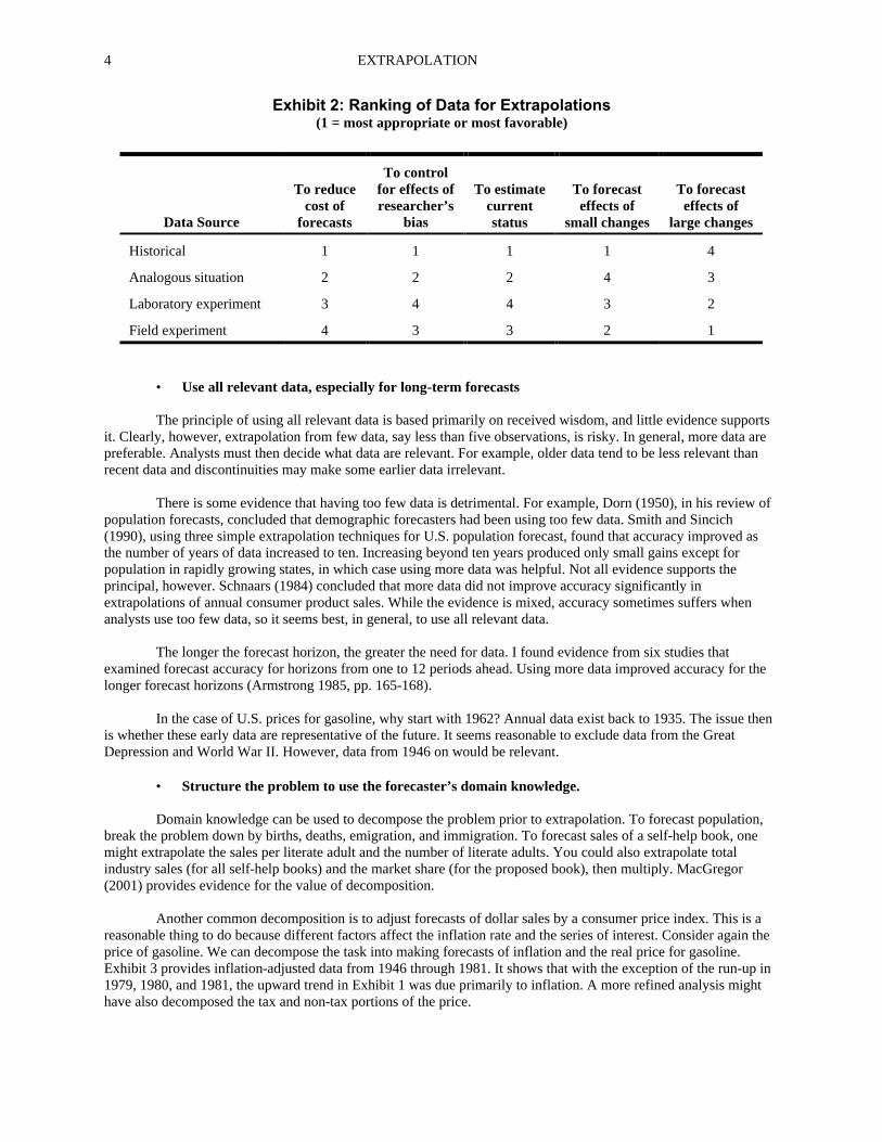
Domain knowledge can be used to decompose the problem prior to extrapolation. To forecast population, break the problem down by births, deaths, emigration, and immigration. To forecast sales of a self-help book, one might extrapolate the sales per literate adult and the number of literate adults. You could also extrapolate total industry sales (for all self-help books) and the market share (for the proposed book), then multiply. MacGregor (2001) provides evidence for the value of decomposition. Another common decomposition is to adjust forecasts of dollar sales by a consumer price index. This is a reasonable thing to do because different factors affect the inflation rate and the series of interest. Consider again the price of gasoline. We can decompose the task into making forecasts of inflation and the real price for gasoline. Exhibit 3 provides inflation-adjusted data from 1946 through 1981. It shows that with the exception of the run-up in 1979, 1980, and 1981, the upward trend in Exhibit 1 was due primarily to inflation. A more refined analysis might have also decomposed the tax and non-tax portions of the price.


5

1.60

0.00

0.20

0.40

0.60

0.80

1.00

1.20

1.40

1945

1950

1955

1960

1965

1970

1975

1980

1985

1990

1995

Exhibit 3U.S. Gasoline Prices

(1982 Dollars)

= Current dollars

= Constant dollars

Source: International Petroleum Encyclopedia, 1999; Tulsa Petroleum Publishing Company

• Clean the data to reduce measurement error.

Real-world data are often inaccurate. Mistakes, cheating, unnoticed changes in definitions, and missing data can cause outliers. Outliers, especially recent ones, can lead to serious forecast errors.

The advice to clean the data applies to all quantitative methods, not just extrapolation. Analysts might

assume that someone has already ensured the accuracy of the data. For example, Nobel Prize recipient Robert Solow assumed that the data reported in his 1957 paper were accurate. These data, drawn from 1909 to 1949, fell along a straight line with the exception that the 1943-1949 data were parallel to the other data but shifted above them. Solow devoted about one-half page to a hypothesis about this “structural shift.” He even drew upon other literature to support this hypothesis. In a comment on Solow’s paper, Hogan (1958) showed that, rather than a “structural shift,” the results were due to mistakes in arithmetic.

Even small measurement errors can harm forecast accuracy. To illustrate the effects of measurement error, Alonso (1968) presented an example in which the current population was estimated to be within one percent of the actual value and the underlying change process was known perfectly. He then calculated a two-period forecast, and the forecast of change had a prediction interval of plus or minus 37 percent. (Armstrong 1985, pp. 459-461, provides a summary of Alonso’s example.) One protection against input errors is to use independent sources of data on the same variable. For example, to estimate the crime rate in an area, you could use police reports and also a survey of residents to see how many were victimized. Large differences would suggest the possibility that one of the measures was inaccurate. If you cannot identify the source of the error, you might use an average of the two measures. If you are working with hundreds of series or more, you need routine procedures to clean the data. One step is to set reasonable limits on the values. For example, sometimes values cannot be negative or go beyond an upper limit. Programs can check for violations of these limits. They can also calculate means and standard deviations, and then show outliers (say with a probability of less than one in a hundred of coming from the same process.) If feasible, you should examine outliers to determine whether they are due to mistakes or to identifiable causes. Graphical procedures may also be useful to examine potential errors in the data. In practice, mistakes in data are common.

EXTRAPOLATION 6

It is wise to modify outliers because they can affect estimates of seasonal factors, levels, and trends. You can reduce outliers to equal the most extreme observation about which you feel confident (Winsorizing). Another procedure is to replace them with the overall mean of the series (excluding outliers) or with a median. For trended data, replace outliers with local averages such as the average of the observations just prior to and just after an outlier. Also, you can make forecasts with the outlier included and then with it replaced by a modified value to assess its effects on forecasts and on prediction intervals.

• Adjust intermittent time series

An intermittent series (also called interrupted series or intermittent demand or irregular demand) is a non-negative series that contains zeros. Such series may reflect a pattern of demand where orders occur in lumps and one or more periods of zero demand ensue. Examples of intermittent demand occur in forecasting the demand for computer components, expensive capital goods, and seasonal goods such as grass seed or snow shovels. Extrapolation methods can encounter difficulties because of the use of zero (especially for series modeled in multiplicative terms) and for the resulting large increases that make it difficult to estimate the trend. There are a number of ways to adjust the series. One way is to aggregate the time-series interval so that it is long enough to rule out intermittent values. For example, if a daily series contains zeros, aggregate to weeks; if a weekly series contains zeroes, aggregate to months; if a monthly series contains zeroes, aggregate to quarters. Aggregation also removes outliers in some series (for cases in which demand shifts from one period to the next). One disadvantage of this approach is that the length of the interval may be longer than desired for decision-making. It also means that updating will be less frequent. Another solution, when working with only a few series, is to replace zero observations with a local average based on the values before and after the zero observation. This enables an analyst to make frequent updates in the system, except for the periods with zero demand. In addition to aggregation across time, one could aggregate across space. For example, instead of looking at county data, look at state data; instead of state data, use national data. However, this may create problems if the decisions are made at the county level. Another approach is to aggregate across similar items. Rather than forecasting for a particular size of a toothpaste brand, data could be aggregated across sizes. Still another solution, known as Croston’s Method, is to use exponential smoothing to estimate two series: one for the time between non-zero values and the other for the values. Details are provided in Croston (1972) with a correction by Rao (1973). Willemain et al. (1994) tested Croston’s method against exponential smoothing. Their tests, which involved artificial and actual data, showed that Croston’s method produced substantially more accurate forecasts of demand per period than were obtained by simply using exponential smoothing. However, this is only a single study. Furthermore, no comparisons have been made on the efficacy of other approaches such as aggregating the data.

• Adjust data for historical events When sporadic events have important effects on historical time-series, you should try to remove their

effects. Such events could include policy changes, strikes, stockouts, price reductions, boycotts, product recalls, or extreme weather. This advice is based primarily on received wisdom. To make subjective adjustments, analysts need good domain knowledge. When similar historical events have occurred often, you should try to obtain quantitative assessments of their impacts on the variable of interest. For example, if a brand uses periodic price reductions, you should estimate their effects on sales and remove them from the data. As noted by Tashman and Hoover (2001), some forecasting software programs have procedures for handling these adjustments. Econometric methods can also be useful here (Allen and Fildes 2001), as can judgmental estimates.

Consider again the rising price of gasoline in the late 1970s. It was caused by collusion among the oil

producers. Received wisdom in economics is that collusion cannot be sustained, and the more participants there are, the more likely it is that cheating will occur. To make a long-range forecast of U.S. gasoline prices, it seems sensible to modify the observations for 1979, 1980, and 1981. Using Winsorizing, one could set the value equal to the highest price observed in the ten years before 1979.


7

SEASONAL ADJUSTMENTS For data reported in periods of less than a year, it is often useful to adjust the data for seasonality. Making seasonal adjustments is an important way to reduce errors in time-series forecasting. For example, in forecasts over an 18-month horizon for 68 monthly economic series from the M-Competition, Makridakis et al. (1984, Table 14) found that seasonal adjustments reduced the MAPE from 23.0 to 17.7 percent. However, Nelson (1972) showed that seasonal adjustments sometimes harm accuracy. Seasonal factors can be estimated by regression analysis where months are represented by dummy variables, or by the relationship between each month and a corresponding moving average (commonly referred to as the ratio-to-moving-average method). Little evidence exists to show that these approaches differ substantially in accuracy, so you might choose between them based on convenience and costs. The ratio-to-moving average is commonly used, although Ittig (1997) claims that, when a trend is present, the seasonal factors contain a systematic error, especially when the trend is multiplicative. Ittig’s evidence for this, however, is not strong. Typically, analysts test seasonal factors and use them only if they are statistically significant. This is a situation where tests of statistical significance seem to be useful.Testing them requires at least three, but preferably five or more years of data. Many software programs require at least three years (Tashman and Hoover 2001). The Census X-12 program (or its predecessor X-11) can be used to estimate seasonal factors. It has provisions for seasonality, trend, adjustments of outliers, trading day adjustments, and differential weighting of observations (Findley, Monsell & Bell 1998; Scott 1997). This program grew from a stream of research initiated by Shiskin, who produced a useful program in the early 1960s (Shiskin 1965). Teams of statisticians have been making improvements since the 1960s. These improvements have helped in identifying historical patterns of seasonality, but they are disappointing for forecasters because they have made the program more difficult to understand, and researchers have done little work to show how the changes affect forecasting. (The program can be downloaded at no charge from the Forecasting Principles site.)

• Use seasonal adjustments if domain knowledge suggests the existence of seasonal fluctuations and if there are sufficient data.

I speculate that seasonal adjustments should be made only when domain experts expect seasonal patterns. Analysts can classify series into three groups: those in which there is no reason to expect seasonality, those in which seasonality might occur, and those expected to have strong seasonal patterns. For some data, such as monthly series for consumer products, almost all series have seasonal patterns. For example, beverage sales can be expected to exhibit strong seasonal patterns because of weather and holidays. For other series, such as data on the stock market, it is difficult to imagine why there would be seasonal patterns; attempts to apply seasonal adjustments for such series will produce false seasonal factors that harm accuracy. When data are lacking, the forecaster might still impose seasonal factors based on domain knowledge. For example, sales of a revolutionary new product for winter sports, garden supplies, or new school supplies will have pronounced seasonality. You could use data from similar products to estimate seasonal factors.

• Use multiplicative seasonal factors if the seasonal pattern is stable, measurement errors are small, the data are ratio-scaled and not near zero, and there are ample data.

Seasonal factors can be stated in multiplicative form (e.g., demand in January is 85% of that in the typical month) or additive (e.g., demand in January is 20,000 units below the average). You should use domain knowledge to decide which is most appropriate. Multiplicative factors are most appropriate when measurement errors are small, data are ample, and the seasonal pattern is stable. Also, multiplicative factors are relevant only for ratio-scaled data and when the observations are not near zero. These conditions commonly occur. If any of these conditions is not met, consider additive factors.

EXTRAPOLATION 8

Multiplicative factors are also useful if you calculate seasonal factors for analogous series (all luxury car sales, for example), and combine these estimates with those from the series itself (e.g., BMW sales). This cannot be done using additive factors.

• Damp seasonal factors when there is uncertainty

Applying seasonal factors can increase forecast errors if there is a great deal of uncertainty in their estimates. Uncertainty in seasonal factors arises in a number of ways. First, the analyst may be uncertain whether the data are subject to seasonal patterns. Second, it may be difficult to adjust for historical events, especially if the pattern varies from year to year. Third, there may be few years of data with which to estimate seasonality; at the extreme, with only one year of data, it would be difficult to distinguish between random variations, trend, and real seasonal effects, and you would not be able to test for statistical significance of the seasonal factors. Fourth, there may be measurement errors in the data. Finally, the longer the forecasting horizon, the more likely the seasonal patterns are to change. To address uncertainty, I suggest damping the seasonal factors. For multiplicative factors, this would involve drawing them in toward 1.0. For example, a damping factor of 0.5 would reduce a seasonal factor of 1.4 to 1.2 (reducing the seasonal impact from 40% to 20%). For additive factors, it would mean drawing them closer to zero. The optimal degree of damping may also depend on the extent to which the trend is damped. Damping can be done in many ways. If it is difficult to adjust for the timing and magnitude of historical events, a local mean or spill-over strategy can be used. Here, a suspected seasonal factor could be modified by using an average of the seasonal factors for the month along with those immediately before and after it. To adjust for measurement error, you can damp the seasonal factors based on the amount of data available. Finally, seasonal factors can be damped based on the length of the horizon, with longer horizons calling for more damping because seasonal patterns might change. Fred Collopy and I conducted a small-scale unpublished study on the accuracy of damped seasonal factors. We selected a stratified random sample of 62 series from the monthly data used in the M-competition. Using our own (limited) domain knowledge, we made rule-based forecasts for one- to 18-month-ahead forecasts with the seasonal adjustment factors from the M-Competition. We repeated the process using damped seasonal factors, again based on limited domain knowledge. For one-month-ahead forecasts, damping reduced the MdAPE by 7.2%. For 18-month-ahead forecasts, damping reduced the error by 5.0%. Damping with a shrinkage modifier (for measurement error) improved accuracy for 66% of the series. Use of a horizon modifier improved accuracy for 56% of the series. These findings, discussed on the Forecasting Principles website, provide mild support for the principle that damped seasonals can improve accuracy. MAKING EXTRAPOLATIONS Once you have prepared the data, you must decide how to extrapolate them. The standard approach has been to decompose the data into level, trend, and cycles. Estimating the Level One source of error in forecasting is inaccurate “nowcasting,” that is, errors in estimating values at the origin of the forecast. This is a problem particularly when using regression based only on the time series. Because the prior data are all weighted equally, the estimate of the current level may be outdated. This problem is more serious for data measured in longer intervals, such as annual rather than monthly data. You can reduce the effects of this problem if you can estimate the trend reliably (or if no trend exists), or by correcting for lag (as suggested by Brown 1959). Another source of errors is large changes that have not yet affected the historical time-series. For example, recent reports carried by the mass media concerning the hazards of a consumer product could harm its sales, but their effects might not yet have been fully reflected in the reported sales data.


9

Statistical procedures may help in setting the starting value (at the beginning of the calibration data). Backwards exponential smoothing was used in the M-Competition (Makridakis et al. 1982). Gardner (1985, p. 1242) achieved accurate forecasts by using regressions to backcast the starting levels. According to the study by Williams and Miller (1999), using either of these rules is more accurate than using the series mean as the starting level and setting the trend to zero. Forecasts of levels are also important when using cross-sectional data. When one lacks knowledge about a particular situation, base rates can be useful. Sometimes base rates have an obvious link to predictions. For example, in trying to predict which cars are likely to be transporting drugs, New Jersey state troopers are unlikely to stop inexpensive cars driven by elderly white women. Other times, domain knowledge might lead to less obvious base rates. Consider the following problem. You have been asked by the U.S. Internal Revenue Service to predict who is cheating on their tax returns. Normally, the IRS predicts cheating based on departures from base rates, such as high charitable contributions. However, Mark Nigrini, an accounting professor, suggested they use a base rate for the digits used in numbers. This uses Benford’s Law, named for the research by Frank Benford in 1938, although similar findings have been traced back to an astronomer, Simon Newcomb, in 1881 (Hill 1998). Benford’s law shows the pattern of numbers that often appear in socio-economic data, especially when the series involve summaries of different series. In Benford’s Law on significant digits, 1’s appears as the first digit 30% of the time and the numbers then decrease steadily until 9, which occurs less than 5% of the time. Cheaters, being unaware of the base rate, are unable to create series that follow Benford’s law. Benford’s Law could also be used to identify those who create false data in corporations’ financial statements (Nigrini 1999).

• Combine estimates of the level Given uncertainty, it makes sense to combine estimates for the level (in year to). This could include

estimates from exponential smoothing, regression, and the random walk. It could also include a subjective estimate when experts have observed large recent changes, especially when they understand their causes and can thus judge whether the changes are temporary or permanent. This principle is based mostly on speculation, although Armstrong (1970), Sanders and Ritzman (2001), Tessier and Armstrong (1977), and Williams and Miller (1999) provide some empirical support. Such combinations can be automated.

Combined estimates are helpful when the measures of level are unreliable. Thus, if one were trying to

predict the outcome of a political election, it would be sensible to combine the results from surveys by different polling organizations or to combine the results from a series of polls over time by a given organization (assuming no major changes had occurred during that time).

Trend Extrapolation

A trend is a trend is a trend, But the question is, will it bend? Will it alter its course Through some unforeseen force And come to a premature end?

Cairncross (1969) Will the trend bend? Some statisticians believe that the data can reveal this. In my judgment, this question can best be answered by domain knowledge. Experts should have a good knowledge of the series and what causes it to vary.

• Use a simple representation of trend unless there is strong contradictory evidence. There are many ways to represent behavior. Researchers seem to be enamored of complex formulations.

However, as Meade and Islam (2001) showed, various sophisticated and well-thought-out formulations often do not improve accuracy. That said, some degree of realism should aid accuracy. For example, economic behavior is typically best represented by multiplicative (exponential) rather than additive (linear) relationships. Sutton (1997) describes why multiplicative relationships represent human behavior well. To use multiplicative trends effectively, you must have ratio-scaled data and small measurement errors.

EXTRAPOLATION 10

The principle of simplicity must be weighed against the need for realism. Complexity should only be used if it is well supported. Simplicity is especially important when few historical data exist or when the historical data are unreliable or unstable.

To assess the value of simplicity, I reviewed empirical evidence on whether you need a method that is more complex than exponential smoothing. Of the 32 studies found, 18 showed no gain in accuracy for complexity, nine showed that simpler methods were more accurate, and only five showed that more complex methods improved accuracy. This summary is based on studies listed in Armstrong (1985, pp. 494-495), excluding those that had been challenged and those that compared exponential smoothing to moving averages. In one of the studies, Schnaars (1984) compared sales forecasts generated by six extrapolation methods for 98 annual time-series. The methods ranged from simple (next year will be the same as this year) to complex (curvilinear regression against time). The forecast horizon ranged from 1 to 5 years, and Schnaars used successive updating to examine almost 1,500 forecasts. The simplest models performed well, especially when there were few historical data and when the historical series seemed unstable. (Stability was assessed just as effectively by subjects who looked at the historical scatter plots as by using auto-correlation or runs statistics). Models that added complexity by squaring the time variable were especially inaccurate. The need for simplicity has been observed in demography over the past half century. In a review of the research, Dorn (1950) found that complex extrapolations were less accurate than simple extrapolations. According to Hajnal’s literature review (1955), crude extrapolations are as accurate as complex ones. Smith’s (1997) review led him to conclude that complexity did not produce more accurate population forecasts. Finally, and of key importance, the M-competition studies have shown that simplicity is a virtue in extrapolation (Makridakis et al. 1982; Makridakis et al. 1993; Makridakis and Hibon 2000). Complex functional forms might be appropriate when you have excellent knowledge about the nature of relationships, the properties of the series are stable through time, measurement errors are small, and random sources of variation are unimportant. This combination of conditions probably occurs infrequently, although it could occur for cross-sectional predictions or for long-term forecasting of annual time series.

• Weight the most recent data more heavily than earlier data when measurement errors are small, forecast horizons are short, and the series is stable.

It seems sensible to weight the most recent data most heavily, especially if measurement errors are unbiased and

small. This is important for short-range forecasts of long-interval data (e.g., one-ahead annual forecasts), because much of the error can arise from poor estimates of levels. Exponential smoothing provides an effective way to do this. Using Brown’s (1962) formulation, for example, the level is estimated from:

where Yt represents the latest value of the series at time t, and tY represents the smoothed average of that series. The " determines how much weight to place on the most recent data: the higher the factor, the heavier the weight. For example, an " of 0.2 would mean that 20 percent of the new average comes from the latest observation, and the other 80 percent comes from the previous average. The weights on each period drop off geometrically. Thus, data from the latest period is weighted by α, data from the period before that by α(1 – α), and data from the observation two periods ago by α(1 – α)2; data of d periods ago would be weighted by α(1 – α)d . You can use a similar procedure for a smoothing factor, beta ($), for the trend calculations, or for a smoothing factor for seasonal factors. If there is a trend in the data, make an adjustment to update the level such as:

tt*

t G)a

a1(YY

−+=

where tG is the smoothed value of the trend. For a comprehensive treatment of exponential smoothing, see Gardner (1985).

1ttt Ya)(1aYY −−+=


11

However, if the series is subject to substantial random measurement errors or to instabilities, a heavy weight on recent data would transmit random shocks to the forecast. These shocks are particularly detrimental to long-term forecasts, that is, after the effects of the short-term instabilities have worn off. In 1981, this would have been a danger for forecasts of gasoline prices.

There is evidence to support the principle to weight recent data more heavily. In one of the earliest studies, Kirby (1966) examined monthly sales forecasts for 23 sewing machine products in five countries using seven and a half years of data where the forecast horizon ranged from one to six months. He compared exponential smoothing with moving averages (the latter did not weight recent data more heavily). For a six-month horizon, the three methods were comparable in accuracy. As he shortened the forecast horizon, however, exponential smoothing became slightly more accurate. Kirby also developed forecasts from artificial data by imposing various types of measurement error upon the original data. He found, for example, that with more random error, moving averages were more accurate than exponential smoothing. This is consistent with the fact that recent errors can transmit shocks to an exponentially smoothed forecast. The M-competition showed exponential smoothing to be more accurate than equally weighted moving averages (Makridakis et al. 1982). For example, in 68 monthly series (their Table 28), the Median APE, averaged over forecast horizons of one to 18 months, was 13.4% for the (untrended) moving average versus 9.0% for the (untrended) exponential smoothing. Exponential smoothing was more accurate over all reported horizons, but its improvements over the moving average were larger for short-term horizons. Similarly, gains were found for 20 annual series (their Table 26); over the forecast horizons from one to six years, the moving average had an error of 13.9% versus 11.5% for exponential smoothing. Gains were observed only for the first three years; the accuracy of the two methods was equal for the last three years.

Should the search for the optimal parameters be tailored to the forecast horizon? This makes sense in that a heavier weight on recent observations is more appropriate for short-term forecasts. On the other hand, such a search reduces the sample size and leads to problems with reliability. Dalrymple and King (1981), in a study of 25 monthly time-series for products and services, found, as might be expected, that the optimum α was larger for short than for long horizons. However, their attempts to optimize smoothing coefficients for each horizon improved accuracy in only one of the eight forecast horizons they examined, and harmed accuracy in six.

• Be conservative when the situation is uncertain

If you ask people to extend a time-series that fluctuates wildly, they will often produce a freehand extrapolation that fluctuates wildly because they want the forecast to look like the historical data. This typically leads to poor forecasts, especially when the forecaster does not understand the reasons for the fluctuations. To the extent that you lack knowledge about the reasons for fluctuations, you should make conservative forecasts. What does it mean to be conservative in forecasting? It varies with the situation, so once again, it is important to draw upon domain knowledge. For example, to be conservative about trends for growth series, you might use additive trends rather than multiplicative (exponential) trends. However, if a series with a natural zero is expected to decay sharply, a multiplicative trend would be more conservative because it damps the trend and because it would not forecast negative values. Using multiplicative trends can be risky for long-range forecasts, so it may be wise to damp the trend. The longer the time horizon, the greater the need for damping. Mark Twain explained what might happen otherwise in Life on the Mississippi:

In the space of one hundred and seventy-six years the Lower Mississippi has shortened itself two hundred and forty-two miles. That is an average of a trifle over one mile and a third per year. Therefore,. . . any person can see that seven hundred and forty-two years from now the Lower Mississippi will be only a mile and three-quarters long, and Cairo and New Orleans will have joined their streets together, and be plodding comfortably along under a single mayor. . . There is something fascinating about science. One gets such wholesale returns of conjecture out of such a trifling investment of fact.

EXTRAPOLATION 12

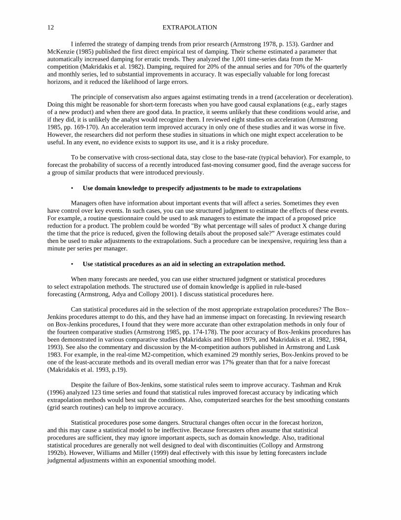
I inferred the strategy of damping trends from prior research (Armstrong 1978, p. 153). Gardner and McKenzie (1985) published the first direct empirical test of damping. Their scheme estimated a parameter that automatically increased damping for erratic trends. They analyzed the 1,001 time-series data from the M-competition (Makridakis et al. 1982). Damping, required for 20% of the annual series and for 70% of the quarterly and monthly series, led to substantial improvements in accuracy. It was especially valuable for long forecast horizons, and it reduced the likelihood of large errors. The principle of conservatism also argues against estimating trends in a trend (acceleration or deceleration). Doing this might be reasonable for short-term forecasts when you have good causal explanations (e.g., early stages of a new product) and when there are good data. In practice, it seems unlikely that these conditions would arise, and if they did, it is unlikely the analyst would recognize them. I reviewed eight studies on acceleration (Armstrong 1985, pp. 169-170). An acceleration term improved accuracy in only one of these studies and it was worse in five. However, the researchers did not perform these studies in situations in which one might expect acceleration to be useful. In any event, no evidence exists to support its use, and it is a risky procedure. To be conservative with cross-sectional data, stay close to the base-rate (typical behavior). For example, to forecast the probability of success of a recently introduced fast-moving consumer good, find the average success for a group of similar products that were introduced previously.

• Use domain knowledge to prespecify adjustments to be made to extrapolations

Managers often have information about important events that will affect a series. Sometimes they even have control over key events. In such cases, you can use structured judgment to estimate the effects of these events. For example, a routine questionnaire could be used to ask managers to estimate the impact of a proposed price reduction for a product. The problem could be worded "By what percentage will sales of product X change during the time that the price is reduced, given the following details about the proposed sale?” Average estimates could then be used to make adjustments to the extrapolations. Such a procedure can be inexpensive, requiring less than a minute per series per manager.

• Use statistical procedures as an aid in selecting an extrapolation method.

When many forecasts are needed, you can use either structured judgment or statistical procedures to select extrapolation methods. The structured use of domain knowledge is applied in rule-based forecasting (Armstrong, Adya and Collopy 2001). I discuss statistical procedures here. Can statistical procedures aid in the selection of the most appropriate extrapolation procedures? The Box–Jenkins procedures attempt to do this, and they have had an immense impact on forecasting. In reviewing research on Box-Jenkins procedures, I found that they were more accurate than other extrapolation methods in only four of the fourteen comparative studies (Armstrong 1985, pp. 174-178). The poor accuracy of Box-Jenkins procedures has been demonstrated in various comparative studies (Makridakis and Hibon 1979, and Makridakis et al. 1982, 1984, 1993). See also the commentary and discussion by the M-competition authors published in Armstrong and Lusk 1983. For example, in the real-time M2-competition, which examined 29 monthly series, Box-Jenkins proved to be one of the least-accurate methods and its overall median error was 17% greater than that for a naive forecast (Makridakis et al. 1993, p.19). Despite the failure of Box-Jenkins, some statistical rules seem to improve accuracy. Tashman and Kruk (1996) analyzed 123 time series and found that statistical rules improved forecast accuracy by indicating which extrapolation methods would best suit the conditions. Also, computerized searches for the best smoothing constants (grid search routines) can help to improve accuracy. Statistical procedures pose some dangers. Structural changes often occur in the forecast horizon, and this may cause a statistical model to be ineffective. Because forecasters often assume that statistical procedures are sufficient, they may ignore important aspects, such as domain knowledge. Also, traditional statistical procedures are generally not well designed to deal with discontinuities (Collopy and Armstrong 1992b). However, Williams and Miller (1999) deal effectively with this issue by letting forecasters include judgmental adjustments within an exponential smoothing model.


13

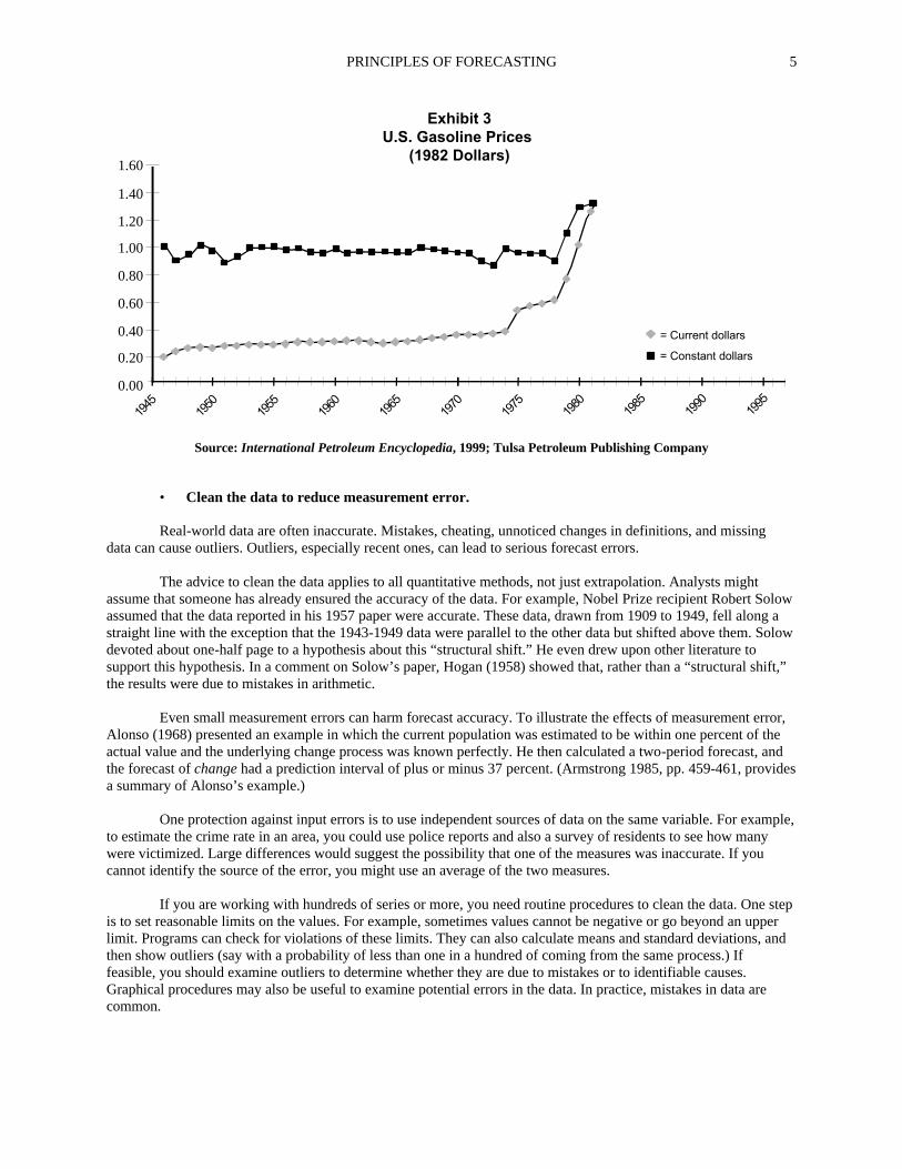
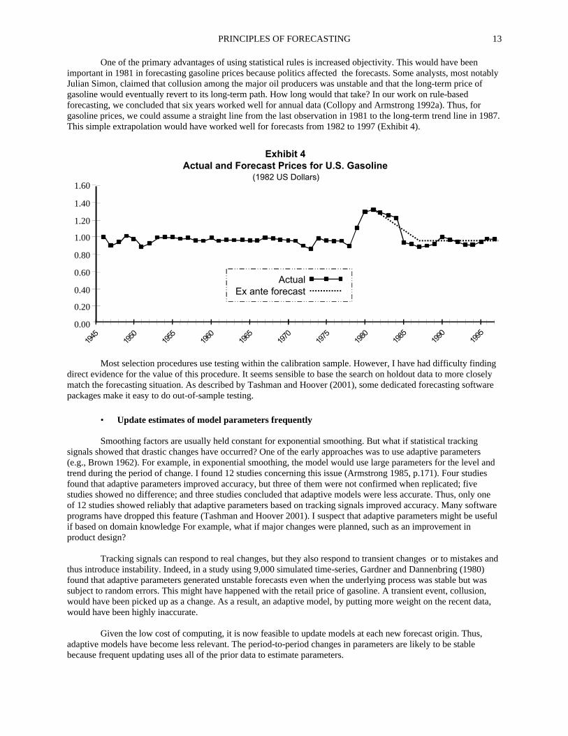
One of the primary advantages of using statistical rules is increased objectivity. This would have been important in 1981 in forecasting gasoline prices because politics affected the forecasts. Some analysts, most notably Julian Simon, claimed that collusion among the major oil producers was unstable and that the long-term price of gasoline would eventually revert to its long-term path. How long would that take? In our work on rule-based forecasting, we concluded that six years worked well for annual data (Collopy and Armstrong 1992a). Thus, for gasoline prices, we could assume a straight line from the last observation in 1981 to the long-term trend line in 1987. This simple extrapolation would have worked well for forecasts from 1982 to 1997 (Exhibit 4).

Exhibit 4Actual and Forecast Prices for U.S. Gasoline

1.60

0.00

0.20

0.40

0.60

0.80

1.00

1.20

1.40

ActualEx ante forecast

1945

1950

1955

1960

1965

1970

1975

1980

1985

1990

1995

(1982 US Dollars)

Most selection procedures use testing within the calibration sample. However, I have had difficulty finding direct evidence for the value of this procedure. It seems sensible to base the search on holdout data to more closely match the forecasting situation. As described by Tashman and Hoover (2001), some dedicated forecasting software packages make it easy to do out-of-sample testing.

• Update estimates of model parameters frequently

Smoothing factors are usually held constant for exponential smoothing. But what if statistical tracking signals showed that drastic changes have occurred? One of the early approaches was to use adaptive parameters (e.g., Brown 1962). For example, in exponential smoothing, the model would use large parameters for the level and trend during the period of change. I found 12 studies concerning this issue (Armstrong 1985, p.171). Four studies found that adaptive parameters improved accuracy, but three of them were not confirmed when replicated; five studies showed no difference; and three studies concluded that adaptive models were less accurate. Thus, only one of 12 studies showed reliably that adaptive parameters based on tracking signals improved accuracy. Many software programs have dropped this feature (Tashman and Hoover 2001). I suspect that adaptive parameters might be useful if based on domain knowledge For example, what if major changes were planned, such as an improvement in product design? Tracking signals can respond to real changes, but they also respond to transient changes or to mistakes and thus introduce instability. Indeed, in a study using 9,000 simulated time-series, Gardner and Dannenbring (1980) found that adaptive parameters generated unstable forecasts even when the underlying process was stable but was subject to random errors. This might have happened with the retail price of gasoline. A transient event, collusion, would have been picked up as a change. As a result, an adaptive model, by putting more weight on the recent data, would have been highly inaccurate.

Given the low cost of computing, it is now feasible to update models at each new forecast origin. Thus, adaptive models have become less relevant. The period-to-period changes in parameters are likely to be stable because frequent updating uses all of the prior data to estimate parameters.

EXTRAPOLATION 14

Clearly it is important to update the level whenever new data are obtained. In effect, this shortens the

forecast horizon and it is well-established that forecast errors are smaller for shorter forecast horizons. In addition, evidence suggests that frequent updating of the parameters contributes to accuracy. Fildes et al. (1998), in a study of 261 telecommunication series, examined forecasts for horizons of one, six, 12, and 18 months, with 1,044 forecasts for each horizon. When they updated the parameters at each forecast horizon (e.g., to provide six-month-ahead forecasts), the forecasts were substantially more accurate than those without updated parameters. Improvements were consistent over all forecast horizons, and they tended to be larger for longer horizons. For example, for damped-trend exponential smoothing, the MAPE was reduced from 1.54% to 1.37% for the one-month-ahead forecasts, a reduction of 11%. For the 18-month-ahead forecasts, its MAPE was reduced from 25.3% to 19.5%, an error reduction of 23%.

Estimating cycles Cycles can be either long-term or short-term. By long-term cycles, I mean those based on observations from annual data over multiple years. By short-term cycles, I mean those for very short periods, such as hourly data on electricity consumption.

• Use cycles when the evidence on future timing and amplitude is highly accurate.

Social scientists are always hopeful that they will be able to identify long-term cycles that can be used to improve forecasting. The belief is that if only we are clever enough and our techniques are good enough, we will be able to identify the cycles. Dewey and Dakin (1947) claimed that the world is so complex, relative to man’s ability for dealing with complexity, that a detailed study of causality is a hopeless task. The only way to forecast, they said, was to forget about causality and instead to find past patterns or cycles. These cycles should then be projected without asking why they exist. Dewey and Dakin believed that economic forecasting should be done only through mechanical extrapolation of the observed cycles. They were unable to validate their claim. Burns and Mitchell (1946) followed the same philosophy in applying cycles to economics. Their work was extended in later years, but with little success. Small errors in estimating the length of a cycle can lead to large errors in long-range forecasting if the forecasted cycle gets out of phase with the actual cycle. The forecasts might also err on the amplitude of the cycle. As a result, using cycles can be risky. Here is my speculation: If you are very sure about the length of a cycle and fairly sure of the amplitude, use the information. For example, the attendance at the Olympic games follows a four-year cycle with specific dates that are scheduled well in advance. Another example is electric consumption cycles within the day. Otherwise, do not use cycles. ASSESSING UNCERTAINTY Traditional approaches to constructing confidence intervals, which are based on the fit of a model to the data, are well reasoned and statistically complex but often of little value to forecasters. Chatfield (2001) reviewed the literature on this topic and concluded that traditional prediction intervals (PIs) are often poorly calibrated for forecasting. In particular, they tend to be too narrow for ex ante time series forecasts (i.e., too many actual observations fall outside the specified intervals). As Makridakis et al. (1987) show, this problem occurs for a wide range of economic and demographic data. It is more serious for annual than for quarterly data, and more so for quarterly than monthly data.

• Use empirical estimates drawn from out-of-sample tests.

The distributions of ex ante forecast errors differ substantially from the distributions of errors when fitting the calibration data (Makridakis and Winkler 1989). (By ex ante forecast errors, we mean errors based on forecasts that go beyond the periods covered by the calibration data and use no information from the forecast periods.) The ex


15

ante distribution provides a better guide to uncertainty than does the distribution of errors based on the fit to historical data. Williams and Goodman (1971) examined seasonally adjusted monthly data on sales of phones for homes and businesses in three cities in Michigan. They analyzed the first 24 months of data by regression on first differences of the data, then made forecasts for an 18-month horizon. They then updated the model and calculated another forecast; they repeated this procedure for 144 months of data. When they used the standard error for the calibration data to establish PIs (using 49 comparisons per series), 81% of the actual values were contained within the 95% PIs. But when they used empirically estimated PIs, 95% of the actual values were within the 95% PIs. Smith and Sincich (1988) examined ten-year-ahead forecasts of U.S. population over seven target years from 1920 to 1980. They calculated empirical PIs to represent the 90% limits. Ninety percent of the actual values fell within these PIs. While it is best to calculate empirical prediction intervals, in some cases this may not be feasible because of a lack of data. The fit to historical data can sometimes provide good calibration of PIs for short-term forecasts of stable series with small changes. For example, Newbold and Granger (1974, p. 161) examined one-month-ahead Box-Jenkins forecasts for 20 economic series covering 600 forecasts and 93% of the actual values fell within the 95% PIs. For their regression forecasts, 91% of the actual values fell within these limits.

• For ratio-scaled data, estimate the prediction intervals by using log transforms of the actual and predicted values.

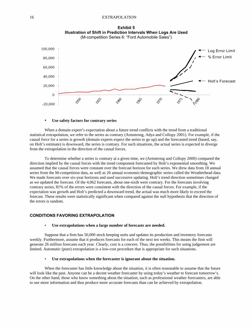
Because PIs are typically too narrow, one obvious response is to make them wider. Gardner (1988) used such an approach with traditional extrapolation forecasts. He calculated the standard deviation of the empirical ex ante errors for each forecast horizon and then multiplied the standard deviation by a safety factor. The resulting larger PIs improved the calibration in terms of the percentage of actual values that fell within the limits. However, widening the PIs will not solve the calibration problem if the errors are asymmetric. The limits will be too wide on one side and too narrow on the other. Asymmetric errors are common in the management and social sciences. In the M-competition (Makridakis et al. 1987), academic researchers used additive extrapolation models. The original errors from these forecasts proved to be asymmetric. For the six-year-ahead extrapolation forecasts using Holt’s exponential smoothing, 33.1% of the actual values fell above the upper 95% limits, while 8.8% fell below the lower 95% limits (see Exhibits 3 and 4 in Makridakis et al. 1987). The results were similar for other extrapolation methods they tested. The corresponding figures for Brown’s exponential smoothing, for example, were 28.2% on the high side and 10.5% on the low side. Although still present, asymmetry occurred to a lesser extent for quarterly data, and still less for monthly data. You might select an additive extrapolation procedure for a variety of reasons. If an additive model has been used for economic data, log transformations should be considered for the errors, especially if large errors are likely. Exhibit 5 illustrates the application of log-symmetric intervals. These predictions of annual Ford automobile sales using Holt’s extrapolation were obtained from the M-competition study (Makridakis et al. 1982, series number 6). We (Armstrong and Collopy 2000) used successive updating over a validation period up to 1967 to calculate the standard 95 percent prediction intervals (dotted lines) from the average ex ante forecast errors for each time horizon. This provided 28 one-year ahead forecasts, 27 two-ahead, and so forth up to 23 six-ahead forecasts. The prediction intervals calculated from percentage errors are unreasonable for the longer forecast horizons because they include negative values (Exhibit 5). In contrast, the prediction intervals calculated by assuming symmetry in the logs were more reasonable (they have been transformed back from logs). The lower level has no negative values and both the lower and upper limits are higher than those calculated using percentage errors.

EXTRAPOLATION 16

Exhibit 5 Illustration of Shift in Prediction Intervals When Logs Are Used

(M-competition Series 6: “Ford Automobile Sales”)

-20,000

0

20,000

40,00019

50

1960

1975

60,000

80,000

100,000

1955

1965

1970

Log Error Limit

% Error Limit

Holt’s Forecast

1980

• Use safety factors for contrary series

When a domain expert’s expectation about a future trend conflicts with the trend from a traditional statistical extrapolation, we refer to the series as contrary (Armstrong, Adya and Collopy 2001). For example, if the causal force for a series is growth (domain experts expect the series to go up) and the forecasted trend (based, say, on Holt’s estimate) is downward, the series is contrary. For such situations, the actual series is expected to diverge from the extrapolation in the direction of the causal forces. To determine whether a series is contrary at a given time, we (Armstrong and Collopy 2000) compared the direction implied by the causal forces with the trend component forecasted by Holt’s exponential smoothing. We assumed that the causal forces were constant over the forecast horizon for each series. We drew data from 18 annual series from the M-competition data, as well as 26 annual economic/demographic series called the Weatherhead data. We made forecasts over six-year horizons and used successive updating. Holt’s trend direction sometimes changed as we updated the forecast. Of the 4,062 forecasts, about one-sixth were contrary. For the forecasts involving contrary series, 81% of the errors were consistent with the direction of the causal forces. For example, if the expectation was growth and Holt’s predicted a downward trend, the actual was much more likely to exceed the forecast. These results were statistically significant when compared against the null hypothesis that the direction of the errors is random. CONDITIONS FAVORING EXTRAPOLATION

• Use extrapolations when a large number of forecasts are needed.

Suppose that a firm has 50,000 stock keeping units and updates its production and inventory forecasts weekly. Furthermore, assume that it produces forecasts for each of the next ten weeks. This means the firm will generate 26 million forecasts each year. Clearly, cost is a concern. Thus, the possibilities for using judgement are limited. Automatic (pure) extrapolation is a low-cost procedure that is appropriate for such situations.

• Use extrapolations when the forecaster is ignorant about the situation. When the forecaster has little knowledge about the situation, it is often reasonable to assume that the future

will look like the past. Anyone can be a decent weather forecaster by using today’s weather to forecast tomorrow’s. On the other hand, those who know something about the situation, such as professional weather forecasters, are able to use more information and thus produce more accurate forecasts than can be achieved by extrapolation.


17

• Use extrapolations when the situation is stable.

Extrapolation is based on an assumption that things will continue to move as they have in the past. This assumption is more appropriate for short-term than for long-term forecasting. In the absence of stability, you could identify reasons for instabilities and then make adjustments. An example of such an instability would be the introduction of a major marketing change, such as a heavily advertised price cut. You could specify the adjustments to be made prior to making the extrapolation, as Williams and Miller (1999) discuss.

• Use extrapolations when other methods would be subject to forecaster bias. Forecasts made by experts can incorporate their biases, which may arise from such things as optimism or

incentives. In such cases, extrapolation offers more objective forecasts, assuming that those forecasts are not subject to judgmental revisions. In the forecasts of gasoline prices (from Exhibit 4), the extrapolation was more accurate than the judgmental forecasts made in 1982, perhaps because it was less subject to bias.

• Use extrapolations as a benchmark in assessing the effects of policy changes. Extrapolations show what is expected if things continue. To assess the potential impact of a new policy,

such as a new advertising campaign, you could describe the changes you anticipate. However, sales might change even without this advertising. To deal with this, you could compare the outcomes you expect with an extrapolation of past data. Gasoline Prices Revisited

Pure extrapolation would have led to forecasts of rapidly rising prices for gasoline. The conditions stated above suggest that pure extrapolation was not ideal for this problem. It failed the first three conditions. However, it did meet the fourth condition (less subject to bias). Through the structured use of domain knowledge, we obtained a reasonable extrapolation of gasoline prices. Is this hindsight bias? Not really. The extrapolation methods follow the principles and use causal forces. They follow the general guideline Julian Simon used in making his 1981 forecasts (Simon 1981, 1985): “I am quite sure that the [real] prices of all natural resources will go down indefinitely.” IMPLICATIONS FOR PRACTITIONERS Extrapolation is the method of choice for production and inventory forecasts, some annual planning and budgeting exercises, and population forecasts. Researchers and practitioners have developed many sensible and inexpensive procedures for extrapolating reliable forecasts. By following the principles, you can expect to obtain useful forecasts in many situations. Forecasters have little need for complex extrapolation procedures. However, some complexity may be required to tailor the method to the many types of situations that might be encountered The assumption underlying extrapolation is that things will continue as they have. When this assumption has no basis, large errors are likely. The key is to identify the exceptions. One exception is situations that include discontinuities. Interventions by experts or a method dependent on conditions, such as rule-based forecasting, are likely to be useful in such cases. Another exception is situations in which trend extrapolations are opposite to those expected. Here you might rely on such alternatives as naive models, rule-based forecasting, expert opinions, or econometric methods. Pure extrapolation is dangerous when there is much change. Managers’ knowledge should be used in such cases. This knowledge can affect the selection of data, the nature of the functional form, and prespecified adjustments. Procedures for using domain knowledge can be easily added to standard extrapolation methods.

EXTRAPOLATION 18

IMPLICATIONS FOR RESEARCHERS Of the thousands of papers published on extrapolation, only a handful have contributed to the development of forecasting principles. We have all heard stories of serendipity in science, but it seems to have played a small role in extrapolation research. Researchers should conduct directed research studies to fill the many gaps in our knowledge about extrapolation principles. For example, little research has been done on how to deal effectively with intermittent series. The relative accuracy of various forecasting methods depends upon the situation. We need empirical research to clearly identify the characteristics of extrapolation procedures and to describe the conditions under which they should be used. For example, researchers could identify time series according to the 28 conditions described by Armstrong, Adya and Collopy (2001). How can we use domain knowledge most effectively and under what conditions do we need it? I believe that integrating domain knowledge with extrapolation is one of the most promising procedures in forecasting. Much is already being done. Armstrong and Collopy (1998) found 47 empirical studies of such methods, all but four published since 1985. Webby, O'Connor and Lawrence (2001) and Sanders and Ritzman (2001) also examine this issue. Rule-based forecasting represents an attempt to integrate such knowledge (Armstrong, Adya and Collopy 2001). SUMMARY Extrapolation consists of many simple elements. Here is a summary of the principles: To select and prepare data:

• Obtain data that represent the forecast situation; • Use all relevant data, especially for long-term forecasts; • Structure the problem to use the forecaster’s domain knowledge; • Clean the data to reduce measurement error; • Adjust intermittent series; and • Adjust data for historical events.

To make seasonal adjustments:

• Use seasonal adjustments if domain knowledge suggests the existence of seasonal fluctuations and if there are sufficient data;

• Use multiplicative factors for stable situations where there are accurate ratio-scaled data; and • Damp seasonal factors when there is uncertainty.

To make extrapolations:

• Combine estimates of the level; • Use a simple representation of trend unless there is strong evidence to the contrary; • Weight the most recent data more heavily than earlier data when measurement errors are small,

forecast horizons are short, and the series is stable; • Be conservative when the situation is uncertain; • Use domain knowledge to provide pre-specified adjustments to extrapolations; • Use statistical procedures as an aid in selecting an extrapolation method; • Update estimates of model parameters frequently; and • Use cycles only when the evidence on future timing and amplitude is highly accurate.


19

To assess uncertainty:

• Use empirical estimates drawn from out-of-sample tests. • For ratio-scaled data, estimate prediction intervals by using log transforms of the actual and

predicted values; and • Use safety factors for contrary series.

Use extrapolations when:

• Many forecasts are needed; • The forecaster is ignorant about the situation; • The situation is stable; • Other methods would be subject to forecaster bias; and • A benchmark forecast is needed to assess the effects of policy changes.

Much remains to be done. In particular, progress in extrapolation will depend on success in integrating judgment, time-series extrapolation can gain from the use of analogous time series, and software programs can play an important role in helping to incorporate cumulative knowledge about extrapolation methods. REFERENCES

Allen, G. & R. Fildes (2001), “Econometric forecasting,” in J. S. Armstrong (ed.), Principles of Forecasting. Norwell, MA:Kluwer Academic Publishers.

Alonso, W. (1968), "Predicting with imperfect data,” Journal of the American Institute of Planners, 34, 248-255.

Armstrong, J. S. (1970), “An application of econometric models for international marketing,” Journal of Marketing Research, 7, 190-198.

Armstrong, J. S. (1978, 1985, 2nd ed.), Long-Range Forecasting: From Crystal Ball to Computer. New York: John Wiley. 1985 edition available in full-text at hops.wharton.upenn.edu/forecast.

Armstrong, J. S., M. Adya & F. Collopy (2001), “Rule-based forecasting: Using judgment in time-series extrapolation,” in J. S. Armstrong (ed.), Principles of Forecasting. Norwell, MA: Kluwer Academic Publishers.

Armstrong, J. S. & F. Collopy (2000), “Identification of asymmetric prediction intervals through causal forces,” Journal of Forecasting (forthcoming).

Armstrong, J. S. & F. Collopy (1998), “Integration of statistical methods and judgment for time-series forecasting: Principles from empirical research,” in G. Wright and P. Goodwin, Forecasting with Judgment. Chichester: John Wiley. Full-text at hops.wharton.upenn.edu/forecast.

Armstrong, J. S. & F. Collopy (1992), “Error measures for generalizing about forecasting methods: Empirical comparisons,” (with discussion), International Journal of Forecasting, 8, 69-111. Full-text at hops.wharton.upenn.edu/forecast.

Armstrong, J. S. & E. J. Lusk (1983), “Research on the accuracy of alternative extrapolation models: Analysis of a forecasting competition through open peer review,” Journal of Forecasting, 2, 259-311 (Commentaries by seven authors with replies by the original authors of Makridakis et al. 1982). Full-text at hops.wharton.upenn.edu/forecast.

Box, G. E. & G. Jenkins (1970; 3rd edition published in 1994), Time-series Analysis, Forecasting and Control. San Francisco: Holden Day.

EXTRAPOLATION 20

Brown, R. G. (1962), Smoothing, Forecasting and Prediction. Englewood Cliffs, N.J.: Prentice Hall.

Brown, R. G. (1959), “Less-risk in inventory estimates,” Harvard Business Review, July-August, 104-116.

Burns, A. F. & W. C. Mitchell (1946), Measuring Business Cycles. New York: National Bureau of Economic Research.

Cairncross, A. (1969), “Economic forecasting,” Economic Journal, 79, 797-812.

Chatfield, C. (2001), “Prediction intervals for time-series,” in J. S. Armstrong (ed.), Principles of Forecasting. Norwell, MA: Kluwer Academic Publishers.

Collopy, F. & J. S. Armstrong (1992a), “Rule-based forecasting: Development and validation of an expert systems approach to combining time series extrapolations,” Management Science, 38, 1374-1414.

Collopy, F. & J. S. Armstrong (1992b), “Expert opinions about extrapolation and the mystery of the overlooked discontinuities,” International Journal of Forecasting, 8, 575-582. Full-text at hops.wharton.upenn.edu/forecast.

Croston, J. D. (1972), “Forecasting and stock control for intermittent demand,” Operational Research Quarterly, 23 (3), 289-303.

Dalrymple, D. J. & B. E. King (1981), “Selecting parameters for short-term forecasting techniques,” Decision Sciences, 12, 661-669.

Dewey, E. R. & E. F. Dakin (1947), Cycles: The Science of Prediction. New York: Holt.

Dorn, H. F. (1950), “Pitfalls in population forecasts and projections,” Journal of the American Statistical Association, 45, 311-334.

Fildes, R., M. Hibon, S. Makridakis & N. Meade (1998), “Generalizing about univariate forecasting methods: Further empirical evidence,” International Journal of Forecasting, 14, 339-358. (Commentaries follow on pages 359-366.)

Fildes, R. & S. Makridakis (1995), “The impact of empirical accuracy studies on time-series analysis and forecasting,” International Statistical Review, 63, 289-308.

Findley, D. F., B. C. Monsell & W. R. Bell (1998), “New capabilities and methods of the X-12 ARIMA seasonal adjustment program,” Journal of Business and Economic Statistics, 16, 127-152.

Gardner, E. S., Jr. (1985), “Exponential smoothing: The state of the art,” Journal of Forecasting, 4, 1-28. (Commentaries follow on pages 29-38.)

Gardner, E. S., Jr. (1988), “A simple method of computing prediction intervals for time-series forecasts,” Management Science, 34, 541-546.

Gardner, E. S., Jr. & D. G. Dannenbring (1980), “Forecasting with exponential smoothing: Some guidelines for model selection,” Decision Sciences, 11, 370-383.

Gardner, E. S., Jr. & E. McKenzie (1985), “Forecasting trends in time-series,” Management Science, 31, 1237-1246.

Groff, G. K. (1973), "Empirical comparison of models for short range forecasting,” Management Science, 20, 22-31.

Hajnal, J. (1955), “The prospects for population forecasts,” Journal of the American Statistical Association, 50, 309-327.


21

Hill, T.P. (1998), “The first digit phenomenon,” American Scientist, 86, 358-363.

Hogan, W. P. (1958), “Technical progress and production functions,” Review of Economics and Statistics, 40, 407-411.

Ittig, P. (1997), “A seasonal index for business,” Decision Sciences, 28, 335-355.

Kirby, R.M. (1966), “A comparison of short and medium range statistical forecasting methods,” Management Science, 13, B202-B210.

MacGregor, D. (2001), “Decomposition for judgmental forecasting and estimation,” in J.S. Armstrong (ed.), Principles of Forecasting. Norwell, MA: Kluwer Academic Publishers.

Makridakis, S., A. Andersen, R. Carbone, R. Fildes, M. Hibon, R. Lewandowski, J. Newton, E. Parzen & R. Winkler (1982), “The accuracy of extrapolation (time-series) methods: Results of a forecasting competition,” Journal of Forecasting, 1, 111-153.

Makridakis, S., A. Andersen, R. Carbone, R. Fildes, M. Hibon, R. Lewandowski, J. Newton, E. Parzen & R. Winkler (1984), The Forecasting Accuracy of Major Time-series Methods. Chichester: John Wiley.

Makridakis, S. & M. Hibon, “The M3-competition: Results, conclusions and implications,” International Journal of Forecasting (forthcoming).

Makridakis, S. & M. Hibon (1979), “Accuracy of forecasting: An empirical investigation,” (with discussion), Journal of the Royal Statistical Society: Series A, 142, 97-145.

Makridakis, S., M. Hibon, E. Lusk & M. Belhadjali (1987), “Confidence intervals,” International Journal of Forecasting, 3, 489-508.

Makridakis, S. & R. L. Winkler (1980), “Sampling distributions of post-sample forecasting errors,” Applied Statistics, 38, 331-342.

Makridakis, S., C. Chatfield, M. Hibon, M. Lawrence, T. Mills, K. Ord & L. F. Simmons (1993), “The M2-Competition: A real-time judgmentally based forecasting study,” International Journal of Forecasting, 9, 5-22. (Commentaries by the authors follow on pages 23-29)

Meade, N. & T. Islam (2001), "Forecasting the diffusion of innovations: Implications for time-series extrapolation,” in J. S. Armstrong (ed.), Principles of Forecasting. Norwell, MA: Kluwer Academic Publishers.

Meese, R. & J. Geweke (1984), “A comparison of autoregressive univariate forecasting procedures for macroeconomic time-series,” Journal of Business and Economic Statistics, 2, 191-200.

Nelson, C.R. (1972), “The prediction performance of the FRB-MIT-Penn model of the U.S. economy,” American Economic Review, 5, 902-917.

Nevin, J. R. (1974), “Laboratory experiments for estimating consumer demand: A validation study,” Journal of Marketing Research, 11, 261-268.

Newbold, P. & C. W. J. Granger (1974), “Experience with forecasting univariate time-series and the combination of forecasts,” Journal of the Royal Statistical Society: Series A, 137, 131-165.

Nigrini, M. (1999), “I’ve got your number,” Journal of Accountancy, May, 79-83.

Rao, A. V. (1973), “A comment on ‘Forecasting and stock control for intermittent demands’,” Operational Research Quarterly, 24, 639-640.

EXTRAPOLATION 22

Reilly, R.R. & G. T. Chao (1982), "Validity and fairness of some alternative employee selection procedures,” Personnel Psychology, 35, 1-62.

Remus, W. & M. O’Connor (2001), “Neural networks for time-series forecasting,” in J. S. Armstrong (ed.), Principles of Forecasting. Norwell, MA: Kluwer Academic Publishers.

Robertson, I. T. & R. S. Kandola (1982), "Work sample tests: Validity, adverse impact and applicant reaction,” Journal of Occupational Psychology, 55, 171-183

Sanders, N. & L. Ritzman (2001), “Judgmental adjustments of statistical forecasts,” in J. S. Armstrong (ed.), Principles of Forecasting. Norwell, MA: Kluwer Academic Publishers.

Schnaars, S. P. (1984), “Situational factors affecting forecast accuracy,” Journal of Marketing Research, 21, 290-297.

Scott, S. (1997), “Software reviews: Adjusting from X-11 to X-12,” International Journal of Forecasting, 13, 567-573.

Shiskin, J. (1965), The X-11 variant of the census method II seasonal adjustment program. Washington, D.C.: U.S Bureau of the Census.

Simon, J. (1981), The Ultimate Resource. Princeton: Princeton University Press.

Simon, J. (1985), “Forecasting the long-term trend of raw material availability,” International Journal of Forecasting, 1, 85-109 (includes commentaries and reply).

Smith, M. C. (1976), "A comparison of the value of trainability assessments and other tests for predicting the practical performance of dental students,” International Review of Applied Psychology, 25, 125-130.

Smith, S. K. (1997), “Further thoughts on simplicity and complexity in population projection models,” International Journal of Forecasting, 13, 557-565.

Smith, S. K. & T. Sincich (1990), “The relationship between the length of the base period and population forecast errors,” Journal of the American Statistical Association, 85, 367-375.

Smith, S. K. & T. Sincich (1988), “Stability over time in the distribution of population forecast errors,” Demography, 25, 461-474.

Solow, R. M. (1957), “Technical change and the aggregate production function,” Review of Economics and Statistics, 39, 312-320.

Sutton, J. (1997), “Gibrat’s legacy,” Journal of Economic Literature, 35, 40-59.

Tashman, L. J. & J. Hoover (2001), “An evaluation of forecasting software,” in J. S. Armstrong (ed.), Principles of Forecasting. Norwell, MA: Kluwer Academic Publishers.

Tashman, L. J. & J. M. Kruk (1996), “The use of protocols to select exponential smoothing procedures: A reconsideration of forecasting competitions,” International Journal of Forecasting, 12, 235-253.

Tessier, T. H. & J. S. Armstrong (1977), “Improving current sales estimates with econometric methods,” Unpublished paper available in full text at hops.wharton.upenn.edu/forecast.

Webby, R., M. O'Connor & M. Lawrence (2001), "Judgmental time-series forecasting using domain knowledge," in J. S. Armstrong (ed.), Principles of Forecasting. Norwell, MA: Kluwer Academic Publishers.


23

Willemain, T. R., C. N. Smart, J. H. Shocker & P. A. DeSautels (1994), “Forecasting intermittent demand in manufacturing: A comparative evaluation of Croston’s method,” International Journal of Forecasting, 10, 529-538.

Williams, D. W. & D. Miller (1999), “Level-adjusted exponential smoothing for modeling planned discontinuities,” International Journal of Forecasting, 15, 273-289.

Williams, W. H. &. L. Goodman (1971), “A simple method for the construction of empirical confidence limits to economic forecasts,” Journal of the American Statistical Association, 66, 752-754.

Acknowledgements: Robert G. Brown, Christopher Chatfield, Fred Collopy, Robert Fildes, Richard H. Franke, Everette S. Gardner, Jr., Robert L. Goodrich, Paul Goodwin, Peter T. Ittig, Johannes Ledolter, Don Miller, J. Keith Ord, Charles N. Smart, Tim Stoughton, Arnold L. Sweet, Leonard J. Tashman and Thomas J. Yokum provided useful comments on early drafts. While there was consensus on the principles, some reviewers have a higher opinion than I do for the value of basic research on extrapolation. Raphael Austin, Ling Qiu and Mariam Rafi provided editorial suggestions.

extrapolation for time-series and cross-sectional data … · · 2017-01-26extrapolation for...

Documents