external cavity mode-locked semiconductor lasers for the
TRANSCRIPT
University of Central Florida University of Central Florida
STARS STARS
Electronic Theses and Dissertations, 2004-2019
2013
External Cavity Mode-locked Semiconductor Lasers For The External Cavity Mode-locked Semiconductor Lasers For The
Generation Of Ultra-low Noise Multi-gigahertz Frequency Combs Generation Of Ultra-low Noise Multi-gigahertz Frequency Combs
And Applications In Multi-heterodyne Detection Of Arbitrary And Applications In Multi-heterodyne Detection Of Arbitrary
Optical Waveforms Optical Waveforms
Josue Davila-Rodriguez University of Central Florida
Part of the Electromagnetics and Photonics Commons, and the Optics Commons
Find similar works at: https://stars.library.ucf.edu/etd
University of Central Florida Libraries http://library.ucf.edu
This Doctoral Dissertation (Open Access) is brought to you for free and open access by STARS. It has been accepted
for inclusion in Electronic Theses and Dissertations, 2004-2019 by an authorized administrator of STARS. For more
information, please contact [email protected].
STARS Citation STARS Citation Davila-Rodriguez, Josue, "External Cavity Mode-locked Semiconductor Lasers For The Generation Of Ultra-low Noise Multi-gigahertz Frequency Combs And Applications In Multi-heterodyne Detection Of Arbitrary Optical Waveforms" (2013). Electronic Theses and Dissertations, 2004-2019. 2526. https://stars.library.ucf.edu/etd/2526
EXTERNAL CAVITY MODE-LOCKED SEMICONDUCTOR LASERS FOR THE
GENERATION OF ULTRA-LOW NOISE MULTI-GIGAHERTZ FREQUENCY COMBS
AND APPLICATIONS IN MULTI-HETERODYNE DETECTION OF ARBITRARY
OPTICAL WAVEFORMS
by
JOSUE DAVILA-RODRIGUEZ
B.S. Tecnologico de Monterrey, 2006
A dissertation submitted in partial fulfillment of the requirements
for the degree of Doctor of Optics
in the College of Optics & Photonics
at the University of Central Florida
Orlando, Florida
Spring Term
2013
Major Professor: Peter J. Delfyett Jr.
ii
© 2013 Josué Dávila-Rodríguez

iii
ABSTRACT
The construction and characterization of ultra-low noise semiconductor-based mode-locked
lasers as frequency comb sources with multi-gigahertz combline-to-combline spacing is studied
in this dissertation. Several different systems were built and characterized. The first of these
systems includes a novel mode-locking mechanism based on phase modulation and periodic
spectral filtering. This mode-locked laser design uses the same intra-cavity elements for both
mode-locking and frequency stabilization to an intra-cavity, 1,000 Finesse, Fabry-Pérot Etalon
(FPE). On a separate effort, a mode-locked laser based on a Slab-Coupled Optical Waveguide
Amplifier (SCOWA) was built. This system generates a pulse-train with residual timing jitter of
<2 fs and pulses compressible to <1 ps. Amplification of these pulse-trains with an external
SCOWA lead to 390 mW of average optical power without evident degradation in phase noise
and pulses that are compressible to the sub-picosecond regime. Finally, a new laser is built using
a 10,000 Finesse Fabry-Pérot Etalon held in a vacuum chamber. The fluctuations in the optical
frequency of the individual comb-lines over time periods longer than 12 minutes are shown to be
significantly reduced to <100 kHz in a measurement that is limited by the linewidth of the
reference source.
The use of these comb sources as local oscillators in multi-heterodyne detection of arbitrary
optical waveforms is explored in three different cases. 1) Sampling of mode-locked pulses, 2)
sampling of phase modulated continuous wave light and 3) periodically filtered white light. The
last experiment achieves spectral interferometry with unprecedented resolution.
iv
"The ancient teachers of this science," said he, "promised impossibilities and
performed nothing. The modern masters promise very little; they know that
metals cannot be transmuted and that the elixir of life is a chimera but these
philosophers, whose hands seem only made to dabble in dirt, and their eyes to
pore over the microscope or crucible, have indeed performed miracles. They
penetrate into the recesses of nature and show how she works in her hiding-
places. They ascend into the heavens; they have discovered how the blood
circulates, and the nature of the air we breathe. They have acquired new and
almost unlimited powers; they can command the thunders of heaven, mimic the
earthquake, and even mock the invisible world with its own shadows."
- M. Waldman (Frankenstein)

v
A mis padres
A Gabo, Becky y Toño
A la flaquita

vi
ACKNOWLEDGMENTS
I owe many thanks to Professor Peter Delfyett for the opportunity to play a small part in his
group. Without his seemingly infinite energy and his truly endless thirst for the next best system
none of what follows would have been possible. Working in the Ultrafast Photonics group has
been a true delight and the experience I’ve gained has shaped the way I approach problems,
reflect upon them and focus on a possible solution. I can only hope that the next hundred or so
pages are a faithful image of the group’s philosophy and work ethic. The members of the group
that I had the privilege to overlap with are: Dr. Frank Quinlan, Dr. Sarper Ozharar, Dr. Ji-
Myoung Kim, Dr. Sangyoun Gee, Dr. Ibrahim Ozdur, Dr. Dimitrios Mandridis, Dr. M.U.
Piracha, Dr. Nazanin Hoghooghi, Chuck Williams-Butt, Sharad Bhooplapur, Abhijeet Ardey,
Dat Nguyen, Marcus Bagnell, Edris Sarailou, Anthony Klee and Kristina Bagnell. Other
colleagues at CREOL that deserve a special mention: Andrew Sims, Andi Eisele, Alessandro
Salandrino, Kyle Douglass, Armando Pérez, Enrique Antonio.
I thank Frank for walking me through the first few experiments and for sharing insights and ideas
even today, many years after he left the group. Ibrahim was always up for hearing my dispersed
and wavy arguments and carefully shooting them down. Dr. Dimitrios Mandridis was the best
person to test argumentative endurance with. Chuck was a great lab partner and the greatest pun-
master. Nazanin was a wonderful colleague and a better friend. She was always willing to listen
and the best at pushing me to do more when I was discouraged.
Finally, I would like to credit the prompt availability of caffeine in CREOL with keeping me
awake through the whole experience.

vii
TABLE OF CONTENTS
LIST OF FIGURES ...................................................................................................................... IX
: INTRODUCTION............................................................................................... 1 CHAPTER 1
1. Applications of frequency combs ............................................................................................ 1
Frequency domain applications .............................................................................................. 2
Time domain applications ....................................................................................................... 5
2. Harmonically mode-locked lasers ........................................................................................... 6
3. Semiconductor-based mode-locked lasers as frequency comb sources ................................ 11
: PHASE NOISE MEASUREMENT TECHNIQUES ........................................ 12 CHAPTER 2
1. Signal representation ............................................................................................................. 12
2. Absolute, relative and residual phase noise .......................................................................... 13
: A MODE-LOCKED LASER STABILIZED TO AN INTRACAVTITY CHAPTER 3
ETALON USING PHASE MODULATION AND PERIODIC OPTICAL FILTERING ........... 19
1. Experimental setup and operation principle .......................................................................... 20
2. Experimental results .............................................................................................................. 25
3. Conclusions ........................................................................................................................... 29
: A MODE-LOCKED LASER USING A SLAB COUPLED OPTICAL CHAPTER 4
WAVEGUIDE AMPLIFIER (SCOWA) AS A GAIN MEDIUM ............................................... 30
1. Experimental setup ................................................................................................................ 31
2. Laser characterization ........................................................................................................... 33
All SMF Cavity ...................................................................................................................... 33
Dispersion compensated cavity ............................................................................................. 37
3. Conclusions ........................................................................................................................... 39
viii
: ALL-DIODE AMPLIFICATION OF 10 GHZ PULSE-TRAINS .................... 41 CHAPTER 5
1. Overall MOPA system .......................................................................................................... 42
2. Experimental results .............................................................................................................. 43
3. Conclusions ........................................................................................................................... 47
: FREQUENCY STABILITY OF A MODE-LOCKED LASER WITH A 10,000 CHAPTER 6
FINESSE FABRY-PEROT ETALON ......................................................................................... 49
1. Experimental setup ................................................................................................................ 49
2. Experimental results .............................................................................................................. 51
3. Amplified spontaneous emission suppression as a function of filter Finesse ....................... 56
4. Conclusions ........................................................................................................................... 57
: APPLICATION OF FREQUENCY COMBS IN MULTI-HETERODYNE CHAPTER 7
MEASUREMENTS. PART I: THEORY ..................................................................................... 58
1. Conceptual description .......................................................................................................... 60
2. Heterodyne detection of bandlimited white light and periodically filtered white light ........ 64
: APPLICATION OF FREQUENCY COMBS IN MULTI-HETERODYNE CHAPTER 8
MEASUREMENTS. PART II: EXPERIMENTAL RESULTS ................................................... 69
1. Mode-locked pulses............................................................................................................... 69
2. Phase modulated light ........................................................................................................... 73
3. White light and periodically filtered white light ................................................................... 78
REFERENCES ............................................................................................................................. 82
ix
LIST OF FIGURES
Figure 1.1: Frequency domain applications of frequency combs. (a) Calibration of stellar
spectrograms and (b) Direct frequency comb spectroscopy using a second frequency comb as a
local oscillator. ................................................................................................................................ 4
Figure 1.2: Optical arbitrary waveform generation using frequency comb from a mode-locked
laser. ................................................................................................................................................ 5
Figure 1.3: Photonically-sampled analog-to-digital converter. The mode-locked pulse-train acts
as the sampling gate in the ADC setup. .......................................................................................... 6
Figure 1.4: Mode-locking through loss modulation. (a) Fundamentally and (b) harmonically
mode-locked lasers.......................................................................................................................... 7
Figure 1.5: Mode-locked pulse-train and the corresponding spectrum. Notice that the fceo has
been chosen to be ¼frep, which can also be seen in the pulses where the peak of the carrier
coincides with the peak of the envelope after four pulses. ............................................................. 8
Figure 1.6. Harmonic mode-locking picture from the perspective of interleaved pulse-trains. In
the top two panels a set of identical pulses are interleaved and perfect coherence makes 3 out of
every 4 comb-lines destructively interfere. In the bottom panels small static phase shifts are
introduced in each pulse-train, generating a periodic pattern in the frequency domain but without
the destructive interference. .......................................................................................................... 10
Figure 2.1: Noise measurement schemes. (a) Relative noise measurement by comparing two
independent oscillators and (b) residual noise measurement. ....................................................... 14
Figure 2.2: Frequency discriminator technique for absolute noise measurements ....................... 16
Figure 2.3: Frequency discriminator transfer function for two different delays. .......................... 18
Figure 3.1: Experimental setup. CIR: Circulator, DBM: Double Balanced Mixer, FPE: Fabry-
Pérot Etalon, ISO: Isolator, LPF: Low-Pass Filter, OC: Output Coupler, PC: Polarization
Controller, PD: Photodetector, PID: Proportional-Integral-Diferential Controller, PM: Phase
Modulator, PS: Phase Shifter, PZT: Piezoelectric Transducer (Fiber Stretcher), SOA:
Semiconductor Optical Amplifier ................................................................................................. 21

x
Figure 3.2: Phase modulation sidebands (black) and FPE transmission peaks (red). The mode-
locking occurs due to the combination of phase modulation and periodic spectral filtering. The
Finesse of the cavity for this plot is F = 100 and the depth of modulation β = 1.84 rad, for
illustration purposes. ..................................................................................................................... 22
Figure 3.3: Measurement of the depth of modulation in the mode-locked laser. The black (red)
dots show the expected amplitudes for depth of modulation = 1.85 rad (2.02 rad). ................. 23
Figure 3.4: Pound-Drever-Hall error signals for several depths of modulation and driving
frequencies. These calculations include the effects of the interaction of higher-order sidebands
with the Fabry-Pérot cavity. .......................................................................................................... 24
Figure 3.5: Measurement of the dynamic PDH slope. (a) Real-time spectrogram and, (b)
recovered peak frequency. The laser remains locked throughout the measurement. An error
signal slope can be calculated from the size of each step, and has been calculated to be ~67
mV/MHz. ...................................................................................................................................... 25
Figure 3.6 – Laser characteristics. (a) Optical spectrum, (b) High-resolution optical spectrum, (c)
Photodetected pulse-train and, (d) Photodetected RF tone. .......................................................... 26
Figure 3.7 – (a) Spectrogram and, (b) a single RF trace of the heterodyne beat between a
continuous-wave laser and one combline of the mode-locked laser. An upper bound to the
frequency stability and the linewidth of the laser comblines can be set from these measurements.
....................................................................................................................................................... 27
Figure 3.8 – Phase noise measurement setup using a regenerative frequency divider. ................ 28
Figure 3.9 – Phase noise power spectral density of the frequency divided radio-frequency tone
and integrated timing jitter. The integrated timing jitter is the same as in the 10.285 GHz signal.
....................................................................................................................................................... 28
Figure 4.1. Mode-locked laser using a SCOWA and an intra-cavity Fabry-Pérot Etalon. CIR:
Circulator, DBM: Double Balanced Mixer, FPE: Fabry-Perot Etalon, ISO: Isolator, LPF: Low-
Pass Filter, OC: Output Coupler (Variable), PC: Polarization controller, PD: Photodetector, PID:
Proportional-Integral-Differential Controller, PM: Phase Modulator, PS: Phase Shifter, PZT:
Piezoelectric Transducer (Fiber Stretcher), SOA: Semiconductor Optical Amplifier (SCOWA),
VOD: Variable Optical Delay ....................................................................................................... 32
xi
Figure 4.2 – (a) Optical spectrum and (b) High-resolution optical spectrum of a single combline.
....................................................................................................................................................... 34
Figure 4.3 – Optical frequency stability measurement via multi-heterodyne detection with a
similarly built laser. (a) Schematic of the experimental setup, (b) Conceptual description of the
multi-heterodyne process and, (c) recorded real-time spectrogram. ............................................. 35
Figure 4.4 – Photodetected pulse-trains (a) directly out of the laser and (b) after external
compression. (c) and (d) show the autocorrelation traces from the pulse-trains in (a) and (b)
respectively. .................................................................................................................................. 35
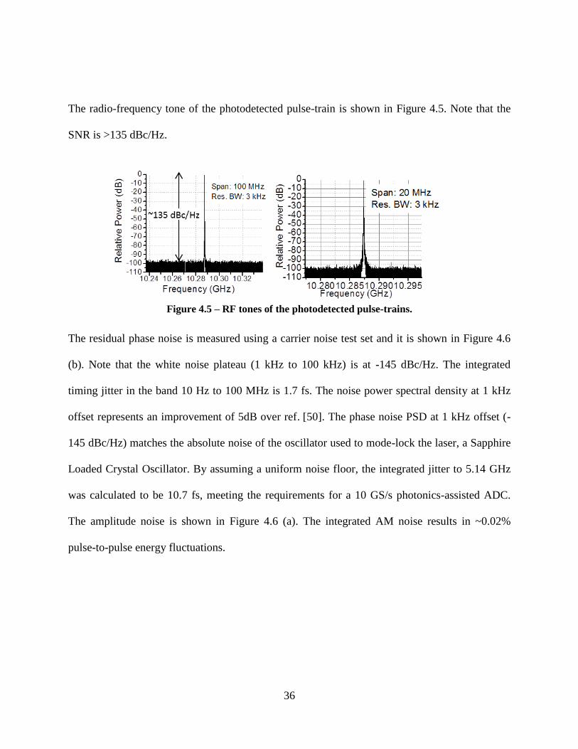
Figure 4.5 – RF tones of the photodetected pulse-trains. ............................................................. 36
Figure 4.6 – (a) Amplitude and (b) phase noise of the 10.287 GHz pulse-train. .......................... 37
Figure 4.7. (a) Optical spectrum of a dispersion compensated laser cavity. (b) Heterodyne beat-
note between a cw laser and a single comb-line. Also shown in (b) are Lorentzian lineshapes
with 1 kHz and 2 kHz FWHM linewidth. ..................................................................................... 38
Figure 4.8. Autocorrelation traces. (a) A comparison of all the compressed autocorrelation traces
in black, from all-SMF cavity, in blue from dispersion compensated cavity and in red, the
calculated transform-limited pulse autocorrelation. (b) A 10 ps span plot showing only the red
and blue traces............................................................................................................................... 38
Figure 4.9. Residual phase noise measurements. The left axis shows the residual phase noise for
(i) this chapter with the all-anomalous dispersion cavity and (ii) the dispersion compensated
cavity; (iii) a similar laser with a commercially available gain medium [50] and (iv) absolute
noise of the mode-locking source for all cases. The noise floor shown corresponds to
measurement (i), but it is comparable in the other cases. The right axis in shows the integrated
timing jitter for curves (i) and (ii) ................................................................................................. 39
Figure 5.1. Overal MOPA system built in the laboratory. The diagnostics box shown in the
dashed box contains standard diagnostics equipment and it is kept as a unit during the
experiments. Phase noise measurements are performed using an attenuated beam both to protect
the photodetector and to match the amount of power used from the original pulse-train. The
dashed box before the amplifier is an optional dispersion stage used to compress the pulses
before amplification. ..................................................................................................................... 43
xii
Figure 5.2. Gain measurements with pulses directly from the cavity and after compression. On
the left side, autocorrelation traces of the pulses input to the amplification stage. On the right side
a plot of Gain vs. Output power for the long (short) pulses in black (red). .................................. 44
Figure 5.3. Optical spectra of the amplified pulse-trains, measured at different output powers.
Amplification of (a) long and (b) short pulses. ............................................................................. 45
Figure 5.4. Pulse autocorrelation traces before and after amplification. (a) Amplifying pulses
directly from the oscillator and subsequently compressing and (b) amplifying compressed pulses.
....................................................................................................................................................... 46
Figure 5.5. Comparison of compressed pulse autocorrelations before (red) and after (blue)
amplification. ................................................................................................................................ 46
Figure 5.6 (a) Phase and (b) amplitude noise measurements for the pulse-trains before (black)
and after (red) amplification ......................................................................................................... 47
Figure 6.1. Schematic of the mode-locked laser utilized in this experiment. CIR: Circulator,
DBM: Double Balanced Mixer, DCF: Dispersion Compensating Fiber, FPE: Fabry-Pérot Etalon,
IM: Intensity Modulator, ISO: isolator, OC: output coupler, PC: Polarization controller, PD:
Photodetector, PBS: Polarizing Beam Splitter, PM: Electro-optic Phase Modulator, PZT:
Piezoelectric Fiber Stretcher, SOA: Semiconductor Optical Amplifier, VOD: Variable Optical
Delay. The PBS used to multiplex the error signal is a bulk component. The FPE is kept in a
vacuum and temperature stabilized enclosure. ............................................................................. 51
Figure 6.2. Characterization of the laser output. (a) Optical Spectrum measured at port B (black)
and port C (red). (b) Autocorrelation traces with the pulses passing through ~20 m of SMF and
~90 m of SMF. In blue, the calculated transform-limited autocorrelation. .................................. 52
Figure 6.3. Multi-heterodyne experimental setup. RT-RFSA: real time Spectrum Analyzer. ..... 53
Figure 6.4. Single trace of the multi-heterodyne spectrum. Each comb-line is clearly resolved.
The following measurements are the result of tracking the 14 comb-lines in the blue box. ........ 54
Figure 6.5. Long term tracking of the comb-line frequency. The data on the left side was taken
on Dec-13-2012 and on the right on Dec-14-2012. The laser operated continuously but it had to
be relocked several times in between. The plotted data shows the beat-note centroid and the error
xiii
bars correspond to ±1σ. Notice that the centroid always remains within a 100 kHz window and
the average value of σ is ~80 kHz................................................................................................. 55
Figure 6.6. Statistics of the beat-note centroid positions. 2xσ is plotted in black squares and the
maximum observed deviation over 12 minutes in red circles. Notice that even the maximum
observed deviations are within one beat-note line-width. ............................................................ 56
Figure 6.7. Broadband ASE suppression for a mode-locked laser using (a) 1,000 Finesse and (b)
10,000 Finesse etalons. ................................................................................................................. 57
Figure 7.1 – Conceptual picture of the multiheterodyne detection with a large repetition rate
detuning. (a) Time domain depiction of the process. Notice the pulse walk-off between the LO
and the signal under test. (b) Frequency domain picture in the optical domain and (c) the
photodetected spectrum of the superposition of the two optical combs. The highest frequency
combline pair (green) illustrates the aliasing effect. This is illustrated by the shaded areas
underneath the frequency axis as well, with an overlapping region. Also note the difference in
scales between the optical and RF frequency axes. ...................................................................... 61
Figure 7.2 – Conceptual experimental setup for white light photocurrent interferometry. .......... 67
Figure 7.3 – Simulation results. (a) Optical spectra. (b) Photocurrent interference for a fixed 20
ns delay ......................................................................................................................................... 68
Figure 8.1 – (a) Optical spectra of the mode-locked comb sources. (b) Photodetected RF
spectrum. (c) Smaller span of the RF spectrum. ........................................................................... 71
Figure 8.2 – Time domain RF waveforms after downconversion as the 10.24 GHz mode-locked
comb experiences different amounts of dispersion. ...................................................................... 72
Figure 8.3 – Experimental setup. Amp: amplifier, BPF: bandpass filter, FC: frequency comb,
CW: CW laser, LPF: low-pass filter, OC: optical coupler, PC: polarization controller, PD:
photodetector, PM: phase modulator, PS: phase shifter, RFC: RF coupler, RFS: RF synthesizer,
VA: variable attenuator. ................................................................................................................ 74
Figure 8.4 – (a) Optical spectra of the phase-modulated CW light and the reference comb. (b)
Photodetected RF spectrum. ......................................................................................................... 74
Figure 8.5 – (a) Time domain waveforms, the red trace is displaced ~1/2 a period with respect to
the black trace. (b) FFT of the fullwaveform. (c) FFT and spectral phase of a 1.6 s segment of
xiv
the waveform. A constant offset and a linear trend have been removed from the phase plot. Only
the phase values where the FFT has significant power are shown. The inset plot shows the errors
of the phase compared to the theoretically expected values. ........................................................ 75
Figure 8.6 – Instantaneous frequency of the photodetected waveform. RF on the left y axis and
optical in the right axis. Notice the compression between the two scales. The rms and mean
absolute error are indicated in the figure. The fit errors are ~5% of the full range. ..................... 76
Figure 8.7 – Fitted time domain waveform. Notice that after a carrier frequency shift and
bandwidth decompression, this corresponds exactly to the phase-modulated optical waveform. 77
Figure 8.8 – Multiheterodyne white light interferometry. (a) Optical spectra of the periodically
filtered white light (blue) and the mode-locked laser (red). (b) RF spectra of the interfering
photocurrents of the downconverted white light. ......................................................................... 79
Figure 8.9 – Spectral interference of downconverted incoherent light. (a) Experimental setup. (b)
Sampled RF waveforms. (c) Power spectra of the sampled waveforms. (d) Spectral interference
with superposed transfer function of a spectral interferometer (red). ........................................... 80
Figure 8.10 – Heterodyne photocurrent interferometry. (a) Experimental setup. (b) Calculated
interferometry spectrogram. (c) Measured interferogram. ........................................................... 81
CHAPTER 1 : INTRODUCTION
Frequency combs have revolutionized a number of fields in experimental physics, metrology and
engineering that their importance can hardly be overstated. A frequency comb, as produced by a
femtosecond mode-locked laser, consists of a large (103 - 10
5) array of equally spaced, phase-
locked narrow frequency components [1,2]. By controlling only two parameters, namely, the
frequency spacing and the carrier-envelope offset frequency, every combline frequency can be
known with sub-Hz accuracy [2,3]. It is this capability makes comb sources invaluable for a
number of applications. This introduction is organized in three sections: the first enumerates and
briefly describes some of the applications of frequency combs, making an attempt at pointing out
which applications benefit from high repetition rate pulse-trains or widely spaced frequency
combs, the second one presents a more detailed description of the frequency comb itself, as
produced by a mode-locked laser, with emphasis on harmonically mode-locked lasers, and the
last section contains a short review of recent advances in semiconductor-based lasers and
frequency comb sources.
1.Applications of frequency combs
The range of applications of optical frequency combs is extremely broad and only a short review
is presented here. Depending on whether the periodicity of the electric field or the spectral purity
and precise equidistancy of the spectral lines is of use to the application at hand one can very
2
broadly (and somewhat artificially, since both characteristics are intimately connected)
categorize the applications of frequency combs into frequency-domain applications and time-
domain applications.
Frequency domain applications
In high precision spectroscopy, an optical frequency comb is used to accurately determine the
optical frequency of the atomic or molecular transition by acting as a link between a microwave
frequency standard and the narrow line-width laser that interrogates said transition [4]. This
ability to essentially count the optical cycles permits extremely precise determinations of the
transition frequencies in single ions [5] and cold atomic beams [6].
This process can be used in reverse using an atomic resonance with very narrow linewidth
(known as a clock transition) as a primary frequency standard and a self-referenced frequency
comb is used to count the optical cycles of the laser interrogating the resonance. The system is
then essentially an optical clock. Optical clocks are expected to perform orders of magnitude
better than the current fountain Cs clock [7,8].
The possibility of extending the spectral coverage of frequency combs via nonlinear processes
also enables molecular spectroscopy in the mid-ir region where the rotational-vibrational
molecular fingerprints lie [9–12]. Molecular fingerprinting with frequency combs could bring
about simple and multiplexed stand-off detection as well as trace gas detection with
unprecedented sensitivities. Nonlinear processes also allow generation of coherent light at the
other end of the electromagnetic spectrum. This is done by generating extremely high peak
electric fields via the control of the carrier-envelope phase slip, which enables coherent high-

3
harmonic generation and has resulted in the generation of extreme UV combs [13] which can
potentially be used for spectroscopy on ionized Helium, extending the tests of Quantum
Electrodynamics [14,15] to a new level of precision.
In the history of scientific progress, the advent of more accurate measurement tools (in this case,
time-keeping and frequency metrology tools) has been accompanied by new scientific
discoveries and technological developments. As an example in fundamental physics, the drift or
fluctuation (or the lack thereof) of fundamental constants can be tested for [16] and more
extreme tests of special and general relativity can be performed by following the changes in the
speed of distant galaxies over time. One technique for detection of extrasolar planets requires the
ability to measure changes in Doppler shifts as small as 1 cm/s/yr [17]. For the measurement of
small Doppler shifts in the emission spectra from distant stars, frequency combs provide a stable
and absolutely calibrated frequency grid that the stellar spectrographs can be compared to. The
absolute calibration provided by the comb allows for comparisons of spectrographs recorded at
distant locations and over very long periods of time without loss of calibration. In essence, this
procedure measures the “wobble” of a star that has an earth-like companion and thus hunt for
possible inhabited extra-solar planets [18,19].

4
Figure 1.1: Frequency domain applications of frequency combs. (a) Calibration of stellar
spectrograms and (b) Direct frequency comb spectroscopy using a second frequency comb as a
local oscillator.
Precision length measurements can be significantly improved by the use of two frequency
combs [20,21], where the coherence in both the RF and optical domains is used to implement a
combined time-of-flight and interferometric measurement which increases the resolution without
decreasing the ambiguity range at the same time. Multi-heterodyne techniques can be also
applied to spectroscopy, using one of the combs as a probe while the second comb acts as a local
oscillator to down-convert and sample the changes undergone by the probe beam. This powerful
technique can simultaneously resolve the individual vibrational-rotational levels in gases and the
signals can be coherently accumulated for very long times, significantly increasing the signal-to-
noise ratio [22–26]. In this dissertation, the application of multi-heterodyne techniques will be
extended to mutually incoherent sources with periodic spectral structures.
Optical communications also benefit from frequency combs by allowing the development of
dense WDM modulation schemes where each combline is modulated individually, the comb
recombined and transmitted through the network [27,28]. Individual lines of lasers with comb
spacing in the order of 10 GHz can be spectrally separated and modulated with high-speed
(b) (a)
5
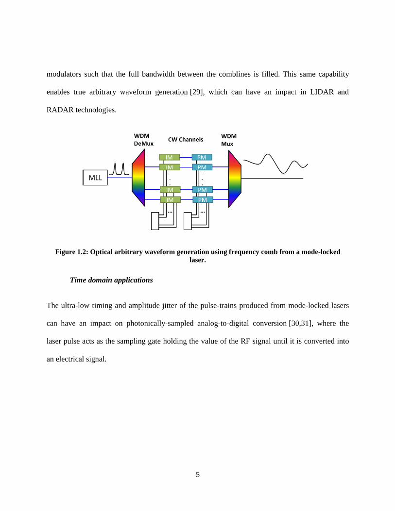
modulators such that the full bandwidth between the comblines is filled. This same capability
enables true arbitrary waveform generation [29], which can have an impact in LIDAR and
RADAR technologies.
Figure 1.2: Optical arbitrary waveform generation using frequency comb from a mode-locked
laser.
Time domain applications
The ultra-low timing and amplitude jitter of the pulse-trains produced from mode-locked lasers
can have an impact on photonically-sampled analog-to-digital conversion [30,31], where the
laser pulse acts as the sampling gate holding the value of the RF signal until it is converted into
an electrical signal.

6
Figure 1.3: Photonically-sampled analog-to-digital converter. The mode-locked pulse-train acts as
the sampling gate in the ADC setup.
More recently, frequency combs have been used in the generation of ultra-low noise microwave
signals via optical frequency division [32–34]. This process requires a self-referenced mode-
locked laser whose repetition rate is locked to an ultra-narrow linewidth continuous wave laser.
The repetition rate of the mode-locked laser is then photodetected and band-pass filtered. The
phase noise of these signals has been shown to be extremely low, since it divides the optical
frequency by a number in the order of 104 to 10
6.
2. Harmonically mode-locked lasers
This section outlines some of the properties of the pulse-trains obtained from fundamentally and
harmonically mode-locked lasers. This topic has been treated extensively in the literature [35–
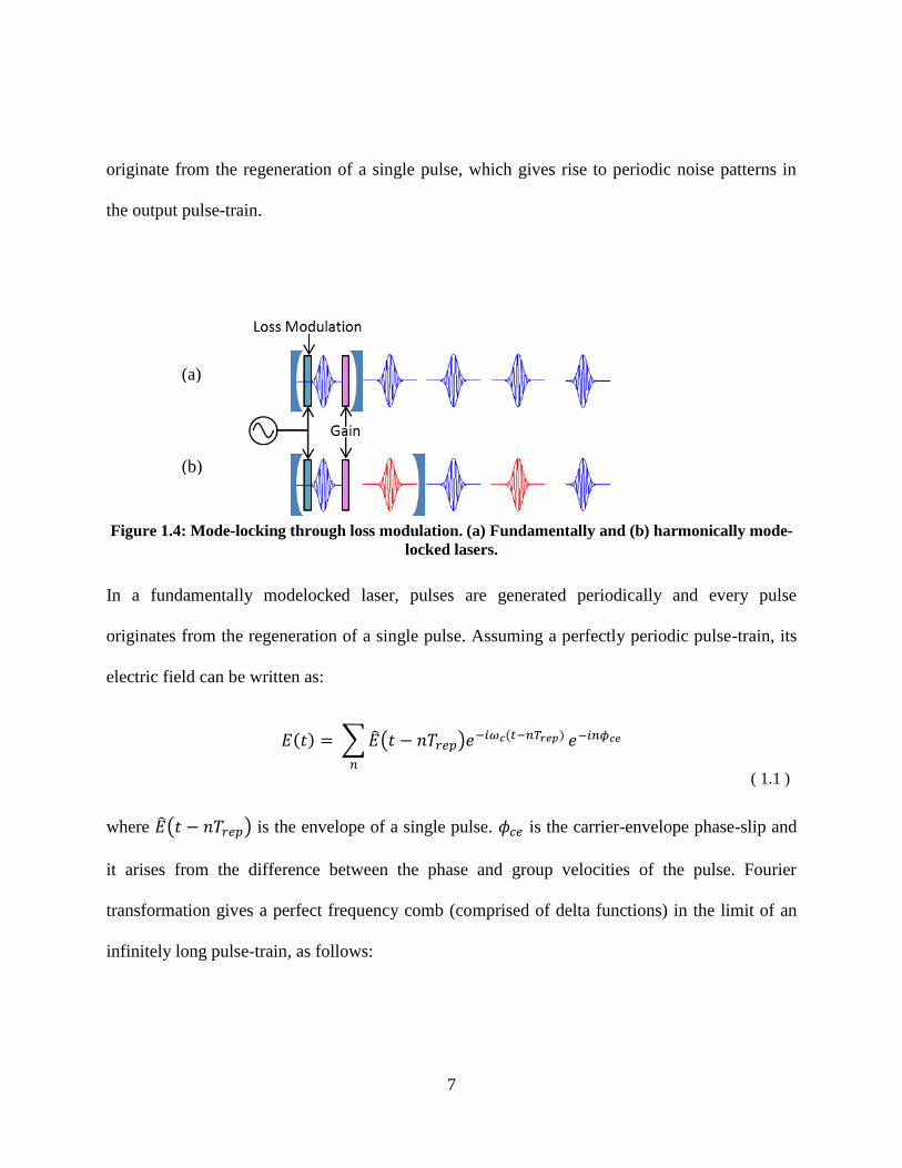
39] and only a brief summary is presented here. A picture of a typical loss-modulation setup for a
mode-locked laser is shown in Figure 1.4, where the modulator in (a) is driven with a period
equal to the round-trip time of the optical cavity or (b) at an integer submultiple of the round-trip
time of the cavity. The pulses in case (b) have been color coded to show that they do not
7
originate from the regeneration of a single pulse, which gives rise to periodic noise patterns in
the output pulse-train.
Figure 1.4: Mode-locking through loss modulation. (a) Fundamentally and (b) harmonically mode-
locked lasers.
In a fundamentally modelocked laser, pulses are generated periodically and every pulse
originates from the regeneration of a single pulse. Assuming a perfectly periodic pulse-train, its
electric field can be written as:
( ) ∑ ( ) ( )
( 1.1 )
where ( ) is the envelope of a single pulse. is the carrier-envelope phase-slip and
it arises from the difference between the phase and group velocities of the pulse. Fourier
transformation gives a perfect frequency comb (comprised of delta functions) in the limit of an
infinitely long pulse-train, as follows:
(a)
(b)
8
( ) ( )∑ ( )
( 1.2 )
where
, and
, and ( ) is the Fourier transform of the envelope of a
single pulse. Therefore, the spectrum is an array of spectral lines located at frequencies equal to:
( 1.3 )
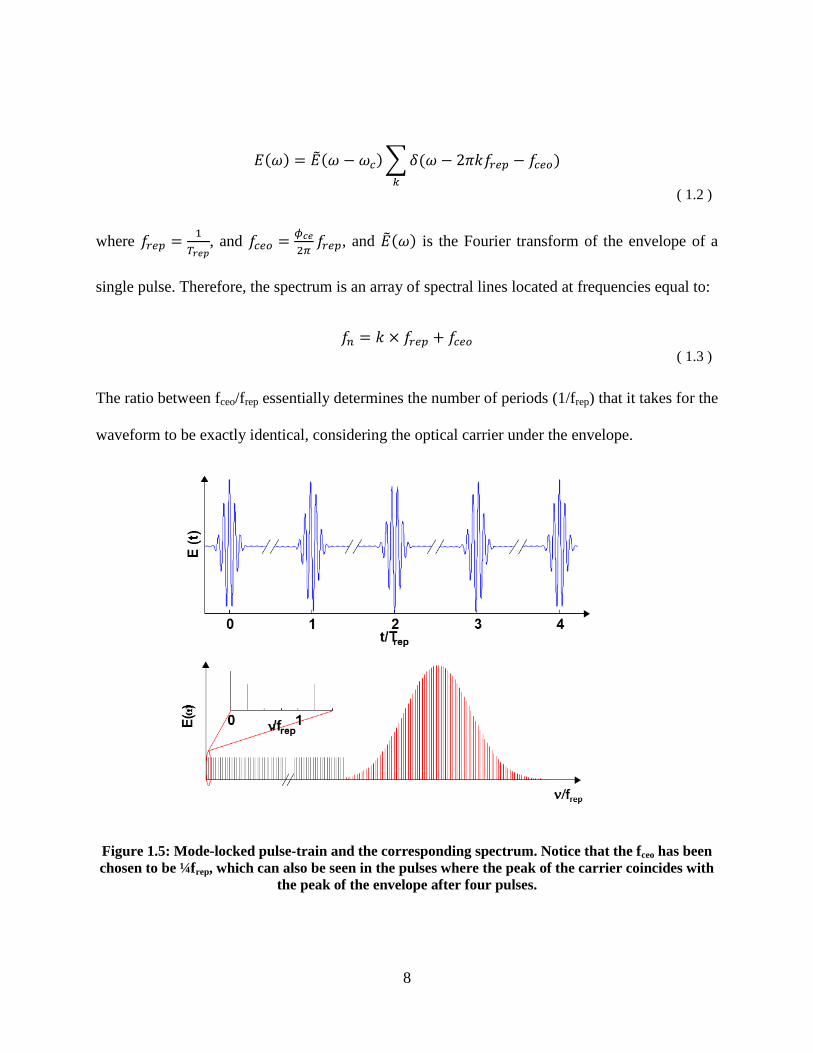
The ratio between fceo/frep essentially determines the number of periods (1/frep) that it takes for the
waveform to be exactly identical, considering the optical carrier under the envelope.
Figure 1.5: Mode-locked pulse-train and the corresponding spectrum. Notice that the fceo has been
chosen to be ¼frep, which can also be seen in the pulses where the peak of the carrier coincides with
the peak of the envelope after four pulses.
9
In a harmonically mode-locked laser, however, there is more than one pulse in the cavity at the
same time (in the case of some of the lasers presented in future chapters, there are 1000’s of
pulses in the cavity). These pulse-trains originate from independent portions of spontaneous
emission and are, in general, not correlated with each other. This property imposes a periodic
noise pattern in the pulse-train with a periodicity equal to the cavity round-trip time. In this
interpretation, the output pulse-train can be considered as the interleaving of multiple
independent pulse-trains, each of which has the period of the cavity round-trip time. This in turn
leads to a spectrum that consists of the summation of independent spectra with comblines spaced
by the cavity fundamental frequency. This picture is shown in Figure 1.6. On the top left side a
high repetition rate pulse-train is represented as the sum of multiple lower repetition rate pulse-
trains. The pulse-trains are assumed to be identical with the exception of a time delay equal to
1/frep between them. This leads to a Fourier transform (top right) where each comb has a different
linear phase slope (everything else is equal). Adding these spectra causes perfect destructive
interference on 3 out of every 4 comb-lines, generating a comb spectrum at the repetition rate of
the pulse-train. This ideal situation is not met in harmonically mode-locked lasers both because
of the presence of dispersion and, more evidently, because each pulse-train is generated from an
‘initial’ burst of amplified spontaneous emission appearing in its time-slot and without
correlation to the other pulse-trains. By assuming that each pulse-train has a random overall
phase shift with respect to the other pulse-trains and adding the obtained spectra (Figure 1.6) the
obtained spectrum has comb-line to comb-line spacing of fcav. Evidently, there is an overall frep
periodicity (both in amplitude and phase) on this comb. This accounts for the high-repetition rate
intensity pattern while the electric field is periodic only with fcav.

10
Figure 1.6. Harmonic mode-locking picture from the perspective of interleaved pulse-trains. In the
top two panels a set of identical pulses are interleaved and perfect coherence makes 3 out of every 4
comb-lines destructively interfere. In the bottom panels small static phase shifts are introduced in
each pulse-train, generating a periodic pattern in the frequency domain but without the destructive
interference.
In the case of an actively mode-locked laser, one can draw a similar picture starting from the
frequency domain due to the fact that the loss modulation imposes a condition which couples
comb-lines that are frep away from each other. Ultimately, this picture leads to a set of pulse-
trains whose repetition rate is equal to frep and which add to generate a pulse-train at the same
repetition rate but whose electric-field phase is periodic with fcav.

11
3.Semiconductor-based mode-locked lasers as frequency comb sources
Semiconductor-based mode-locked lasers can be very attractive as compact sources of
picosecond pulses with high repetition rates in the fiber optic communication band of 1.5
µm [40]. Semiconductor laser media are also attractive because they are electrically pumped,
which contributes to the compactness of the system, as well as to its wall-plug efficiency.
Although the integration of light emitting semiconductor chips with CMOS compatible
technologies (to achieve full optical-electronic integration) remains a field that faces many
challenges, significant improvements have been made over the past few years [41,42] and it can
certainly be expected that more integrated devices will be developed in the near future.
Ultra-stable and ultra-low noise performance of semiconductor lasers can be achieved with
external cavities, through careful cavity engineering and design. Long term stabilization of pulse
repetition rate and optical frequency has been demonstrated through the use of intra-cavity
etalons and Pound-Drever-Hall control loops [35,43].
Finally, another advantage of semiconductors-based lasers is that their operation can be extended
to other wavelength regimes via bandgap engineering.

12
CHAPTER 2 : PHASE NOISE MEASUREMENT TECHNIQUES
This chapter will introduce some of the techniques used in the measurement of fluctuations in
periodic signals. Several techniques previously developed in the domain of microwaves [44–46]
can be imported and adapted to the field of optics since the photodetected current corresponds to
a microwave electrical signal that carries the timing and amplitude jitter of the envelope of the
original pulse-train. Other methods, such as frequency discriminators, benefit from optics and
can be improved and used in a much broader spectral region using optical fibers and
interferometric techniques [47,48], as will be discussed below. In general, it is relevant to
understand the significance of noise, its fundamental limits and the techniques to measure and
characterize it.
1.Signal representation
A narrow-band signal can be represented as a sinusoid whose amplitude and phase are allowed to
present small deviations from the ideal case. This representation can be done in a Cartesian
manner using in-phase and quadrature components or, in a phasor fashion, using amplitude and
phase. The latter is convenient since the fluctuations in these quantities represent the amplitude
and timing jitter of the signal. Thus, an almost perfect sinusoid can be represented as:
( ) {[ ( )] ( ( ))} [ ( )] ( ( )) ( 2.1 )
where α(t) represents the fractional amplitude fluctuations and φ(t) the phase fluctuations. The
signal is written normalized to unitary amplitude and an overall constant phase has been omitted

13
by setting the time origin at one of the maxima of the signal. Although both amplitude and phase
noise are assumed to be small, phase noise and amplitude noise are fundamentally different in
that, for long observation times, phase noise diverges, whereas amplitude noise is bound in every
oscillator by some limiting mechanism.
The spectral content of such a signal can be obtained through its Fourier transform as follows:
( )
√ ∫ [ ( )] ( ) ( )
( 2.2 )
Assuming φ(t) << 1 radian and α(t) << 1, expanding the phase noise from the exponential and
ignoring all higher-order noise terms, we can rewrite this integral as
( )
√ ∫ [ ( ) ( )] ( )
( 2.3 )
where it is evident that the first-order noise terms appear as sidebands on a delta function
centered at ω0. Amplitude noise and phase noise appear as an in-phase and in-quadrature
addition, respectively. Higher order phase noise terms as well as mixing products do appear in
the expansion, but can usually be ignored provided that the noise is small, which is always the
case for a high-quality oscillator.
2.Absolute, relative and residual phase noise
Amplitude and phase fluctuations can be measured in several ways that are relevant depending
on the particular application. Power spectral densities of either α(t) or φ(t) are usually measured
14
using a radio-frequency spectrum analyzer (RFSA) or a similar device. Measuring directly at the
carrier frequency has some drawbacks: (1) an RFSA measures power spectral densities,
combining phase and amplitude fluctuations, (2) the noise sidebands are usually extremely small
compared to the carrier such that the dynamic range of the RFSA is not enough, (3) the IF filter
bandwidth is usually much larger than would be desired and (4) the swept voltage controlled
oscillator inside the RFSA can be too unstable for the task. Down-conversion with a mixer solves
most of these problems by allowing the mixing to be done with an arbitrary phase angle
(separating AM and PM noise) and producing the noise sidebands at close-to-zero frequencies,
which makes it easy to accurately sample and analyze together with a second harmonic term
which can be easily filtered out. Since timing jitter is probably the most important parameter in
the stability of an oscillator, the descriptions given here will be centered on phase noise. Also,
the experimental setups described are conceptual in nature and some practical issues will be
discussed later.
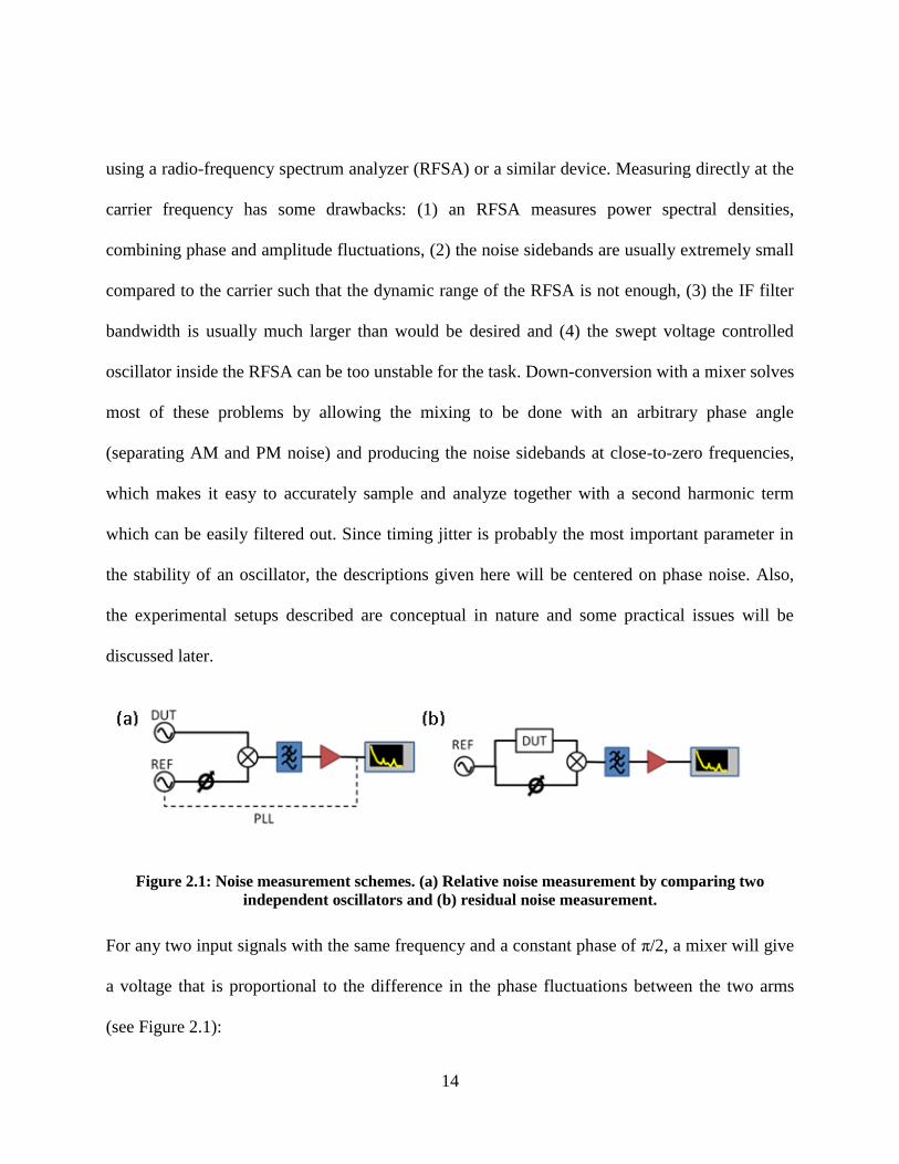
Figure 2.1: Noise measurement schemes. (a) Relative noise measurement by comparing two
independent oscillators and (b) residual noise measurement.
For any two input signals with the same frequency and a constant phase of π/2, a mixer will give
a voltage that is proportional to the difference in the phase fluctuations between the two arms
(see Figure 2.1):

15
( ) ( ) ( ) ( 2.4 )
The power spectral density of this signal would then be:
( ) ( ) ( ) { { ( ) ( )}} ( 2.5 )
where the last term in the expression is the Fourier transform of the cross correlation of the phase
fluctuations of both sources and for uncorrelated devices this term vanishes. Each of the first two
terms represents the absolute noise of each signal and it measures the deviation of the phase of
the signal from that of a perfect sinusoid, while the measured quantity, Sv(ω), is known as the
relative noise between the sources. The ultimate performance of an oscillator is given by its
absolute noise. Figure 2.1 (a) shows a conceptual measurement setup of this type. If the reference
oscillator’s phase noise is much lower than that of the device under test (DUT) then the output
noise is approximately that of the DUT. If they are similar, then the noise is twice that of a single
oscillator. It is evident from Eq. ( 2.4 ) that in a residual noise measurement the fluctuations that
are common to both oscillators will interfere due to coherent addition of signals. For very short
path differences or low Fourier frequencies, these quantities destructively interfere and vanish.
Residual noise is used to mean the uncorrelated noise added by the DUT. In the case of mode-
locked lasers this includes spontaneous emission and the environmental noise that modifies the
properties of the laser cavity. Figure 2.1 (b) shows a residual noise measurement, where it is
evident that the fluctuations of the reference source will cancel out, as long as they are not
filtered by the DUT. If the DUT includes a high-finesse filter, then the measurement will yield
artificially high residual noise in the spectral regions where the phase noise in the DUT arm is
16
lower than the phase noise in the reference arm [49]. The total noise of a two-port device would
be given by:
( ) ( ) ( ) ( ) ( 2.6 )
where h(t) is the impulse response of the DUT and φres(t) is the residual (uncorrelated) noise
added by the device. The power spectral density of the output of the mixer would then be:
( ) [ ( )] ( ) ( )
( 2.7 )
The cross correlation term was omitted from Eq. ( 2.7 ) since the residual noise is by definition
uncorrelated to the noise of the reference. From this equation it is also evident that in the spectral
regions where H(ω) is flat, the output of the mixer is the residual noise of the device.
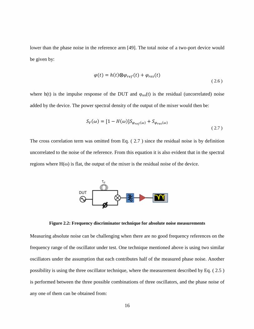
Figure 2.2: Frequency discriminator technique for absolute noise measurements
Measuring absolute noise can be challenging when there are no good frequency references on the
frequency range of the oscillator under test. One technique mentioned above is using two similar
oscillators under the assumption that each contributes half of the measured phase noise. Another
possibility is using the three oscillator technique, where the measurement described by Eq. ( 2.5 )
is performed between the three possible combinations of three oscillators, and the phase noise of
any one of them can be obtained from:
17
( )
[ ( ) ( ) ( )]
( 2.8 )
The main disadvantage of the three oscillator method is that it requires the three oscillators of
comparable quality. Another method for absolute noise measurements consists of the frequency
discriminator or delay-line measurement, schematically shown in Figure 2.2. In this setup, the
signal is mixed with a delayed version of itself, causing the noise at different frequency offsets to
interfere in a periodic fashion [47,48]. It is easy to see that:
{ ( ) ( )}
[ ] { ( )}
( 2.9 )
From this equation, we can see that the phase noise of the oscillator and the power spectral
density at the output of the mixer are related by:
( ) ( ) ( ) ( 2.10 )
The frequency discriminator transfer function is shown in Figure 2.3. For this particular
measurement system, it is advantageous to use a photonic (fiber) delay line because it minimizes
the losses; it is practically immune to electromagnetic interference and can be very compact. It is
important to note that the noise at low frequency offsets is severely attenuated due to the transfer
function of the delay line. Thus, to measure long term stability of oscillator, long delay lines are
required and high stability for these fiber coils must be ensured as well.

18
Figure 2.3: Frequency discriminator transfer function for two different delays.
A common figure of merit for the performance of oscillators is the integrated rms timing jitter,
which can be calculated from the phase noise power spectral density through:
√ ∫ ( )
( 2.11 )
In the following chapters, the residual timing jitter of actively mode-locked lasers will be used as
a figure of merit to assess the quality of the pulse-train as it compares to the mode-locked source.
19
CHAPTER 3 : A MODE-LOCKED LASER STABILIZED TO AN
INTRACAVTITY ETALON USING PHASE MODULATION AND
PERIODIC OPTICAL FILTERING
Both high repetition rate pulse-trains and frequency comb sources with multi-gigahertz
combline-to-combline spacing are desirable for a multiplicity of applications [27,28].
Harmonically mode-locked lasers can directly provide high repetition rate pulse-train, but have
the drawback that multiple cavity mode-sets may exist at the same time and this leads to periodic
noise patterns in the output pulse-trains [35–37]. To overcome this issue, harmonically mode-
locked lasers with an intra-cavity Fabry-Pérot etalon (FPE) as a high-finesse filter have been
demonstrated and have shown good performance in regards to amplitude and phase noise of the
output optical pulse-trains as well as the frequency stability of the individual comblines [50].
This architecture has the advantage that the long fiber cavity has a high quality factor, providing
narrow longitudinal modes, while the FPE provides the wide mode-spacing. In these comb
sources, the modes of the fiber cavity are stabilized to the intra-cavity FPE through a modified,
multi-combline, Pound-Drever-Hall (PDH) scheme. The PDH stabilization loop typically
requires an independent radio-frequency source in order to phase modulate a portion of the
output optical comb and derive an error signal by probing the FPE resonance through a technique
analogous to frequency modulation spectroscopy [51,52]. However, there is a trade-off between
the optical power available as usable laser output and that used in the stabilization loop. Since
the slope of the error signal increases with the optical power, using a larger fraction of the light
in the stabilization loop results in a tighter lock, but this reduces the power available in the output

20
pulse-train. Increasing the output coupling makes more power available for the PDH loop at the
expense of the laser's cavity quality factor.
Mode-locked lasers using phase modulation and an intra-cavity FPE have been demonstrated as
a means for repetition rate multiplication [53,54]. These lasers operate by modulating at a sub-
harmonic of the etalon’s FSR. It is then the higher order side-bands that oscillate in the cavity,
creating pulse-trains with a repetition rate that is a multiple of the driving frequency.
In this chapter, a mode-locked laser is presented in which both mode-locking and frequency
stabilization are achieved using a single phase modulator and the intra-cavity etalon. Using the
same intra-cavity elements for both purposes achieves a simplification of the feedback loop that
is typically used, as compared to the one in reference [50]. It should be noted that in this setup
(Figure 3.1), all of the intra-cavity power is used for the stabilization loop, which is roughly an
order of magnitude larger than the output power, creating tighter lock while avoiding the trade-
off with the available power at the output.
1.Experimental setup and operation principle
A commercially available semiconductor optical amplifier (SOA) is used as the gain medium
and the phase modulator is driven at exactly one-half the free-spectral range (FSR) of the FPE.
The etalon is built with an ultra-low expansion quartz spacer, is hermetically sealed to mitigate
the effects of environmental fluctuations, and has FSR = 10.285 GHz and a Finesse of 1,000. The
fiber cavity is 28 m long and is comprised entirely of standard single mode fiber. Mode-locking
21
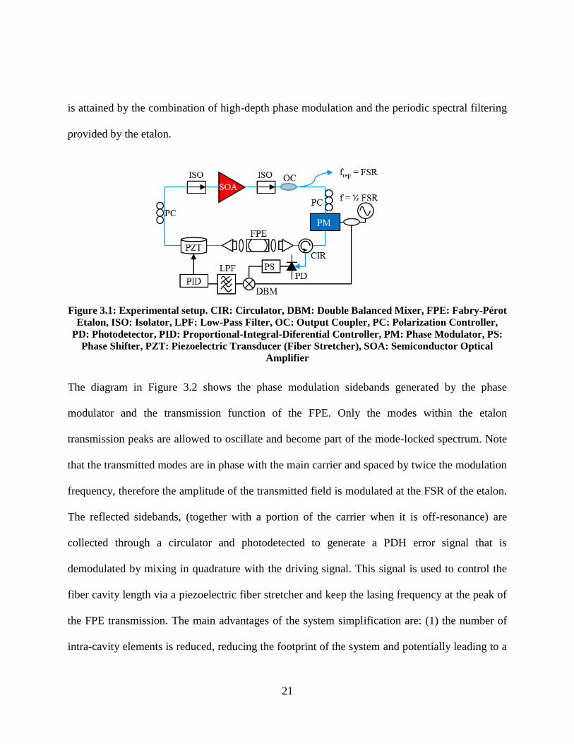
is attained by the combination of high-depth phase modulation and the periodic spectral filtering
provided by the etalon.
Figure 3.1: Experimental setup. CIR: Circulator, DBM: Double Balanced Mixer, FPE: Fabry-Pérot
Etalon, ISO: Isolator, LPF: Low-Pass Filter, OC: Output Coupler, PC: Polarization Controller,
PD: Photodetector, PID: Proportional-Integral-Diferential Controller, PM: Phase Modulator, PS:
Phase Shifter, PZT: Piezoelectric Transducer (Fiber Stretcher), SOA: Semiconductor Optical
Amplifier
The diagram in Figure 3.2 shows the phase modulation sidebands generated by the phase
modulator and the transmission function of the FPE. Only the modes within the etalon
transmission peaks are allowed to oscillate and become part of the mode-locked spectrum. Note
that the transmitted modes are in phase with the main carrier and spaced by twice the modulation
frequency, therefore the amplitude of the transmitted field is modulated at the FSR of the etalon.
The reflected sidebands, (together with a portion of the carrier when it is off-resonance) are
collected through a circulator and photodetected to generate a PDH error signal that is
demodulated by mixing in quadrature with the driving signal. This signal is used to control the
fiber cavity length via a piezoelectric fiber stretcher and keep the lasing frequency at the peak of
the FPE transmission. The main advantages of the system simplification are: (1) the number of
intra-cavity elements is reduced, reducing the footprint of the system and potentially leading to a

22
cavity design with lower loss, (2) an additional RF oscillator is not needed for the stabilization
loop, and (3) the useful output power is increased since there is no need to use a portion of it in
the stabilization loop.
Figure 3.2: Phase modulation sidebands (black) and FPE transmission peaks (red). The mode-
locking occurs due to the combination of phase modulation and periodic spectral filtering. The
Finesse of the cavity for this plot is F = 100 and the depth of modulation β = 1.84 rad, for
illustration purposes.
A few parameters must be optimized to obtain the desired laser performance. The depth of
modulation was empirically optimized based on laser performance (optical bandwidth and pulse-
train stability). Keeping the RF power to the phase modulator constant and using a CW laser, a
measurement was performed to obtain the depth of modulation. The plot in Figure 3.3 shows the
High Resolution optical spectrum of the output from the phase modulator. This measurement
shows that the depth of modulation is between 1.85 and 2 rad. It is important to note that this
range of depth of modulation is with certainty below the point ( = 2.405 rad) at which the
carrier is suppressed and it is in fact close to the point where the first and second order sidebands
have the same power. It was also found that the laser can mode-lock (and be PDH locked) at
lower modulation indices, typically at the cost of narrower spectral bandwidth.

23
Figure 3.3: Measurement of the depth of modulation in the mode-locked laser. The black (red) dots
show the expected amplitudes for depth of modulation = 1.85 rad (2.02 rad).
The standard PDH stabilization scheme assumes a relatively low depth of modulation (to be able
to consider only first order side-bands in the calculation) and that the generated side-bands are
non-resonant. Neither condition is fulfilled in this setup because the depth of modulation is high,
leading to considerable power in higher-order sidebands and, all the even order sidebands are
resonant with the Fabry-Pérot cavity. For this reason, numerical calculations were performed to
verify that an error signal could be obtained. Figure 3.4 shows the calculated error signals for
several cases. To point out some of the interesting features of these calculations, notice that when
the modulation index increases significantly (middle column) several structures appear from the
interaction of the resonant even-order sidebands. Another interesting case is when the carrier is
completely suppressed ( = 2.405), where no error signal is observed on resonance, signal that
reappears as the modulation frequency reaches ½FSR, at which point the signal originates from
the interaction of the ±2 sidebands.
194.36 194.37 194.38 194.39 194.4 194.41 194.42 194.43 194.44-60
-50
-40
-30
-20
-10
0
Frequency (THz)
Op
tic
al
Po
we
r (d
Bm
)
Measurement
= 1.85
= 2.02
24
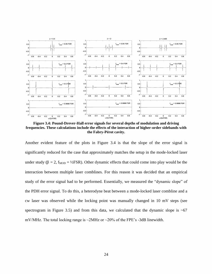
Figure 3.4: Pound-Drever-Hall error signals for several depths of modulation and driving
frequencies. These calculations include the effects of the interaction of higher-order sidebands with
the Fabry-Pérot cavity.
Another evident feature of the plots in Figure 3.4 is that the slope of the error signal is
significantly reduced for the case that approximately matches the setup in the mode-locked laser
under study ( = 2, fMOD = ½FSR). Other dynamic effects that could come into play would be the
interaction between multiple laser comblines. For this reason it was decided that an empirical
study of the error signal had to be performed. Essentially, we measured the “dynamic slope” of
the PDH error signal. To do this, a heterodyne beat between a mode-locked laser combline and a
cw laser was observed while the locking point was manually changed in 10 mV steps (see
spectrogram in Figure 3.5) and from this data, we calculated that the dynamic slope is ~67
mV/MHz. The total locking range is ~2MHz or ~20% of the FPE’s -3dB linewidth.

25
Figure 3.5: Measurement of the dynamic PDH slope. (a) Real-time spectrogram and, (b) recovered
peak frequency. The laser remains locked throughout the measurement. An error signal slope can
be calculated from the size of each step, and has been calculated to be ~67 mV/MHz.
2.Experimental results
The mode-locked laser output consists of a pulse-train with 10.285 GHz repetition rate and
average power of ~5 mW. The optical spectrum is a comb of optical frequencies spaced by
10.285 GHz and has a 10 dB bandwidth of ~3 nm (Figure 3.6(a)). A high resolution trace of one
combline is shown in Figure 3.6 (b). The modes spaced by the cavity fundamental (~7 MHz) are
not visible in this measurement. The observed optical signal to noise ratio is 60 dB at a resolution
bandwidth of 1 MHz. An average of 12 sampling oscilloscope traces of the corresponding pulse-
train is shown in Figure 3.6 (c), using an oscilloscope with equivalent bandwidth of 30 GHz. The
photodetected RF tone at 10.285 GHz in Figure 3.6 (d) has signal-to-noise ratio >115 dBc/Hz.
(b) (a)
26
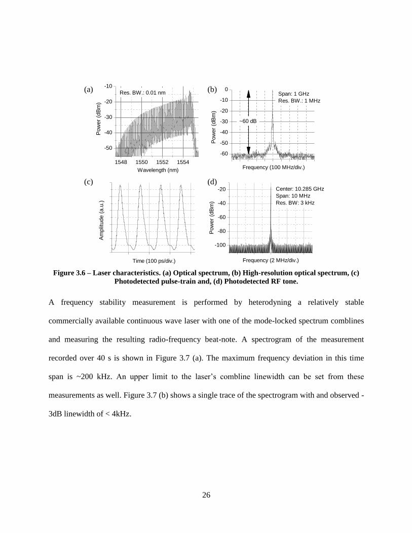
Figure 3.6 – Laser characteristics. (a) Optical spectrum, (b) High-resolution optical spectrum, (c)
Photodetected pulse-train and, (d) Photodetected RF tone.
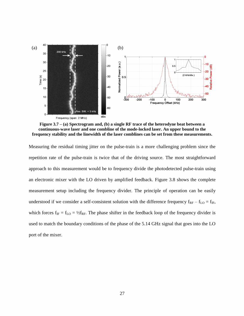
A frequency stability measurement is performed by heterodyning a relatively stable
commercially available continuous wave laser with one of the mode-locked spectrum comblines
and measuring the resulting radio-frequency beat-note. A spectrogram of the measurement
recorded over 40 s is shown in Figure 3.7 (a). The maximum frequency deviation in this time
span is ~200 kHz. An upper limit to the laser’s combline linewidth can be set from these
measurements as well. Figure 3.7 (b) shows a single trace of the spectrogram with and observed -
3dB linewidth of < 4kHz.
1548 1550 1552 1554
-50
-40
-30
-20
-10
Wavelength (nm)
Pow
er
(dB
m)
Res. BW.: 0.01 nm
-60
-50
-40
-30
-20
-10
0
Pow
er
(dB
m)
Frequency (100 MHz/div.)
Span: 1 GHz
Res. BW.: 1 MHz
~60 dB
Am
plit
ude (
a.u
.)
Time (100 ps/div.)
-100
-80
-60
-40
-20
Pow
er
(dB
m)
Frequency (2 MHz/div.)
Center: 10.285 GHz
Span: 10 MHz
Res. BW: 3 kHz
(b) (a)
(c) (d)
27
Figure 3.7 – (a) Spectrogram and, (b) a single RF trace of the heterodyne beat between a
continuous-wave laser and one combline of the mode-locked laser. An upper bound to the
frequency stability and the linewidth of the laser comblines can be set from these measurements.
Measuring the residual timing jitter on the pulse-train is a more challenging problem since the
repetition rate of the pulse-train is twice that of the driving source. The most straightforward
approach to this measurement would be to frequency divide the photodetected pulse-train using
an electronic mixer with the LO driven by amplified feedback. Figure 3.8 shows the complete
measurement setup including the frequency divider. The principle of operation can be easily
understood if we consider a self-consistent solution with the difference frequency fRF – fLO = fIF,
which forces fIF = fLO = ½fRF. The phase shifter in the feedback loop of the frequency divider is
used to match the boundary conditions of the phase of the 5.14 GHz signal that goes into the LO
port of the mixer.
(a) (b)
28
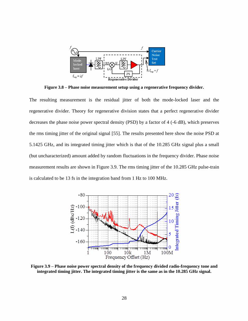
Figure 3.8 – Phase noise measurement setup using a regenerative frequency divider.
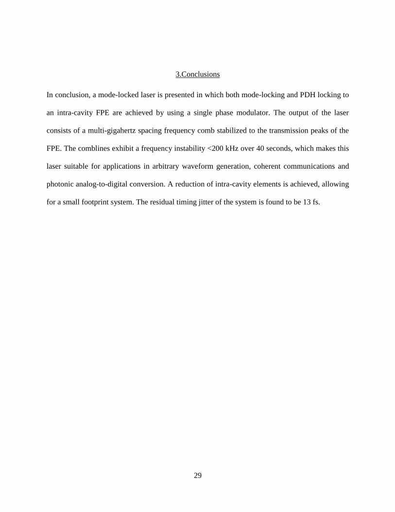
The resulting measurement is the residual jitter of both the mode-locked laser and the
regenerative divider. Theory for regenerative division states that a perfect regenerative divider
decreases the phase noise power spectral density (PSD) by a factor of 4 (-6 dB), which preserves
the rms timing jitter of the original signal [55]. The results presented here show the noise PSD at
5.1425 GHz, and its integrated timing jitter which is that of the 10.285 GHz signal plus a small
(but uncharacterized) amount added by random fluctuations in the frequency divider. Phase noise
measurement results are shown in Figure 3.9. The rms timing jitter of the 10.285 GHz pulse-train
is calculated to be 13 fs in the integration band from 1 Hz to 100 MHz.
Figure 3.9 – Phase noise power spectral density of the frequency divided radio-frequency tone and
integrated timing jitter. The integrated timing jitter is the same as in the 10.285 GHz signal.
29
3.Conclusions
In conclusion, a mode-locked laser is presented in which both mode-locking and PDH locking to
an intra-cavity FPE are achieved by using a single phase modulator. The output of the laser
consists of a multi-gigahertz spacing frequency comb stabilized to the transmission peaks of the
FPE. The comblines exhibit a frequency instability <200 kHz over 40 seconds, which makes this
laser suitable for applications in arbitrary waveform generation, coherent communications and
photonic analog-to-digital conversion. A reduction of intra-cavity elements is achieved, allowing
for a small footprint system. The residual timing jitter of the system is found to be 13 fs.
30
CHAPTER 4 : A MODE-LOCKED LASER USING A SLAB COUPLED
OPTICAL WAVEGUIDE AMPLIFIER (SCOWA) AS A GAIN MEDIUM
Optical frequency combs with multi-gigahertz spacing are useful in applications such as optical
arbitrary waveform generation (OAWG) [29,56,57], ultrafast signal processing [27,28], high
resolution spectroscopy [23,25], and astronomical spectrograph calibration [18]. In the time
domain these sources produce low-noise high-repetition-rate pulse-trains that can be used in high
speed analog-to-digital conversion (ADC) [30,31,58,59], and the generation of ultra-low noise
microwaves [33,34,60,61]. Low pulse-to-pulse amplitude and timing fluctuations are key to
many of these applications. For example, a photonically sampled ADC at 10 GS/s requires a
timing jitter smaller than 12 fs and under 0.03% of amplitude noise to operate with 10 effective
bits of resolution [30].
It has been shown that low noise semiconductor-based harmonically mode-locked lasers can
produce stable frequency combs with a cavity design that uses a long optical fiber cavity with a
nested Fabry-Pérot etalon (FPE) [50]. In this architecture, the narrow linewidth of the individual
comblines is due to the long storage time of the fiber cavity (and thus, its more stringent
frequency selectivity), while the wide comb spacing is due to the spacing between the periodic
transmission peaks of the intra-cavity etalon. In this chapter, we describe experiments performed
to include a Slab-Coupled Optical Waveguide Amplifier (SCOWA) in a harmonically mode-
locked laser with an intracavity etalon to further improve its performance. Additionally, a Pound-
Drever-Hall loop is incorporated to stabilize the comb to the transmission peaks of the etalon.
31
This setup locks the fiber cavity fundamental frequency to a subharmonic of the etalon or,
equivalently, its optical path length to an integer multiple of the round trip length of the etalon.
1.Experimental setup
The experimental setup is shown in Figure 4.1. An optical cavity with 5 MHz free spectral range
(corresponding to 40 m of single mode optical fiber) is built around a Fabry-Pérot etalon with a
finesse of 103. The laser is mode-locked via loss modulation using an intra-cavity LiNbO3 Mach-
Zehnder modulator driven by an ultra-low noise microwave oscillator. The modulator is driven at
10.287 GHz, to closely match the free-spectral range of the FPE. The mode-locked comb is
locked to the FPE’s transmission peaks through a Pound-Drever-Hall (PDH) loop, shown in the
shaded box in Figure 4.1. The PDH loop consists on phase modulating the output comb at 500
MHz and reinjecting this phase-modulated comb in the FPE in an orthogonal polarization state.
The reflected sidebands are photodetected and mixed with the 500 MHz tone to recover a signal
that is proportional to the frequency difference between the transmission peak of the FPE and the
comblines. This signal is then used to feed back into the fiber cavity length through a piezo-
electric fiber stretcher. This loop essentially locks the fiber cavity fundamental frequency to a
subharmonic of the FPE’s free spectral range (FSR), or its optical path length to an integer
multiple of the FPE’s double-pass distance. A variable output coupler is used to optimize output
coupling ratio. Furthermore, dispersion compensating fiber (DCF) is inserted in the cavity to
make an attempt at increasing the spectral bandwidth of the output comb. Results for both the
all-SMF and the dispersion compensated cavity are described in this chapter.
32
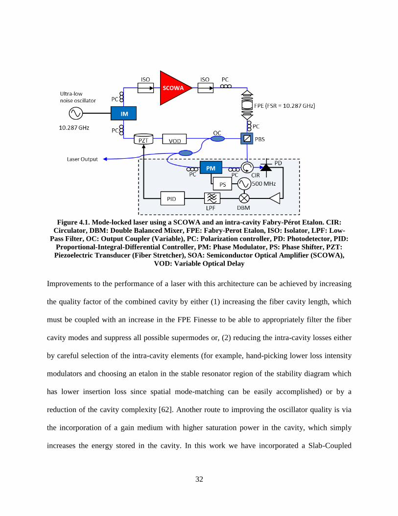
Figure 4.1. Mode-locked laser using a SCOWA and an intra-cavity Fabry-Pérot Etalon. CIR:
Circulator, DBM: Double Balanced Mixer, FPE: Fabry-Perot Etalon, ISO: Isolator, LPF: Low-
Pass Filter, OC: Output Coupler (Variable), PC: Polarization controller, PD: Photodetector, PID:
Proportional-Integral-Differential Controller, PM: Phase Modulator, PS: Phase Shifter, PZT:
Piezoelectric Transducer (Fiber Stretcher), SOA: Semiconductor Optical Amplifier (SCOWA),
VOD: Variable Optical Delay
Improvements to the performance of a laser with this architecture can be achieved by increasing
the quality factor of the combined cavity by either (1) increasing the fiber cavity length, which
must be coupled with an increase in the FPE Finesse to be able to appropriately filter the fiber
cavity modes and suppress all possible supermodes or, (2) reducing the intra-cavity losses either
by careful selection of the intra-cavity elements (for example, hand-picking lower loss intensity
modulators and choosing an etalon in the stable resonator region of the stability diagram which
has lower insertion loss since spatial mode-matching can be easily accomplished) or by a
reduction of the cavity complexity [62]. Another route to improving the oscillator quality is via
the incorporation of a gain medium with higher saturation power in the cavity, which simply
increases the energy stored in the cavity. In this work we have incorporated a Slab-Coupled
33
Optical Waveguide Amplifier (SCOWA) as a gain medium. SCOWAs have shown excellent
performance with respect to high saturation power and low noise figure [63–65].
It should be noted that incorporating a SCOWA as the gain medium in this type of cavities is
challenging due to the fact that SCOWAs typically have lower gain compared to commercially
available devices, which considerably reduces the available loss budget. As an example, it would
have been practically impossible to realize this laser using a flat-flat FPE, since the fiber-to-fiber
insertion loss is typically high (~7dB). On the other hand, by using a cavity with curved mirrors,
a stable resonator is achieved and the mode can be matched very closely using simple optics,
which allows for coupling losses of ~1 dB or less.
The cavity dispersion is roughly matched first by inserting a low-loss patchcord of DCF that is
longer than the estimated required value and then the dispersion is matched by interchanging
SMF fiber lengths and optimizing the laser performance at each step until the largest bandwidth
is obtained. The rationale behind this iterative procedure of varying the length of SMF instead of
DCF is that given the lower absolute value of the dispersion of SMF makes it simpler to change
the dispersion by a smaller amount per step.
2.Laser characterization
All SMF Cavity
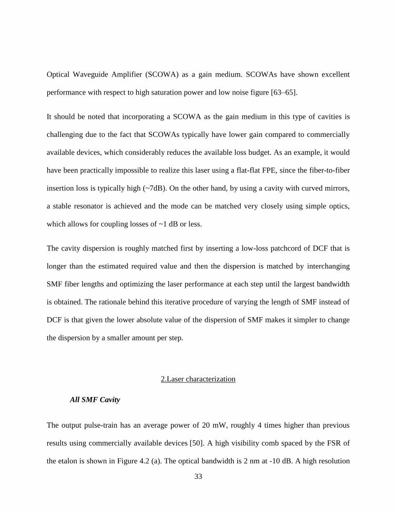
The output pulse-train has an average power of 20 mW, roughly 4 times higher than previous
results using commercially available devices [50]. A high visibility comb spaced by the FSR of
the etalon is shown in Figure 4.2 (a). The optical bandwidth is 2 nm at -10 dB. A high resolution
34
measurement of a single combline is shown in Figure 4.2 (b). Notice that the optical SNR is >60
dB, limited by the noise floor of the High Resolution Spectrum Analyzer.
Figure 4.2 – (a) Optical spectrum and (b) High-resolution optical spectrum of a single combline.
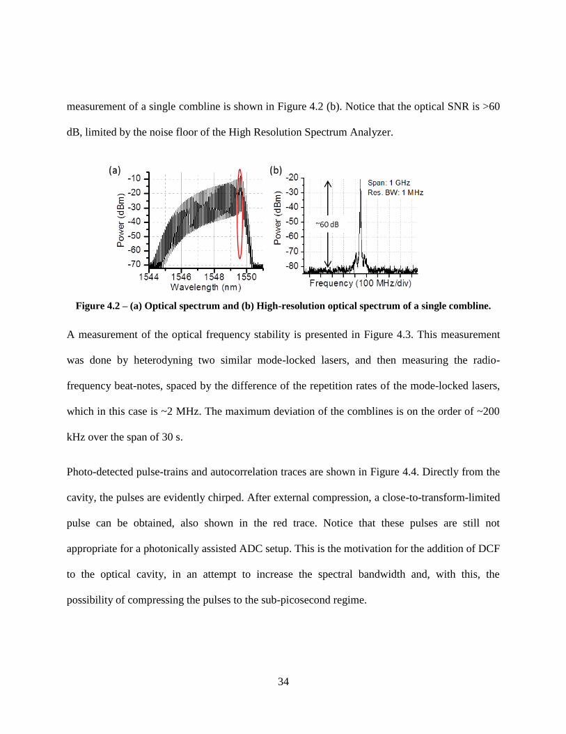
A measurement of the optical frequency stability is presented in Figure 4.3. This measurement
was done by heterodyning two similar mode-locked lasers, and then measuring the radio-
frequency beat-notes, spaced by the difference of the repetition rates of the mode-locked lasers,
which in this case is ~2 MHz. The maximum deviation of the comblines is on the order of ~200
kHz over the span of 30 s.
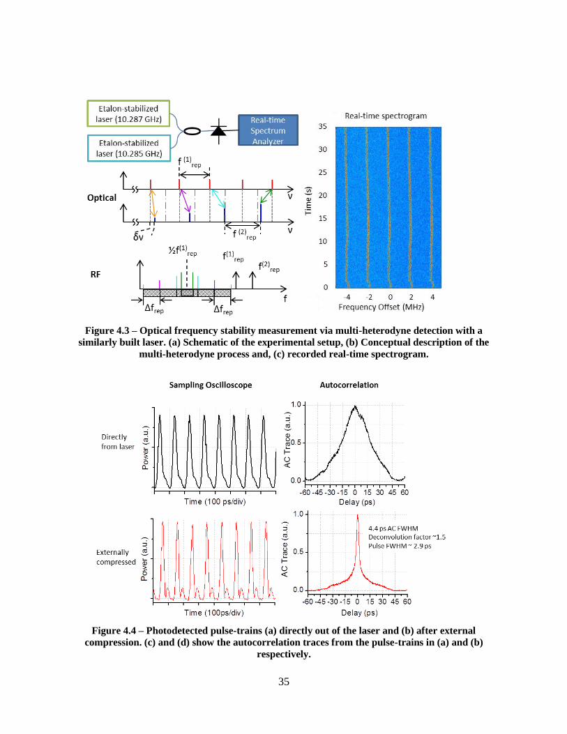
Photo-detected pulse-trains and autocorrelation traces are shown in Figure 4.4. Directly from the
cavity, the pulses are evidently chirped. After external compression, a close-to-transform-limited
pulse can be obtained, also shown in the red trace. Notice that these pulses are still not
appropriate for a photonically assisted ADC setup. This is the motivation for the addition of DCF
to the optical cavity, in an attempt to increase the spectral bandwidth and, with this, the
possibility of compressing the pulses to the sub-picosecond regime.
35
Figure 4.3 – Optical frequency stability measurement via multi-heterodyne detection with a
similarly built laser. (a) Schematic of the experimental setup, (b) Conceptual description of the
multi-heterodyne process and, (c) recorded real-time spectrogram.
Figure 4.4 – Photodetected pulse-trains (a) directly out of the laser and (b) after external
compression. (c) and (d) show the autocorrelation traces from the pulse-trains in (a) and (b)
respectively.
36
The radio-frequency tone of the photodetected pulse-train is shown in Figure 4.5. Note that the
SNR is >135 dBc/Hz.
Figure 4.5 – RF tones of the photodetected pulse-trains.
The residual phase noise is measured using a carrier noise test set and it is shown in Figure 4.6
(b). Note that the white noise plateau (1 kHz to 100 kHz) is at -145 dBc/Hz. The integrated
timing jitter in the band 10 Hz to 100 MHz is 1.7 fs. The noise power spectral density at 1 kHz
offset represents an improvement of 5dB over ref. [50]. The phase noise PSD at 1 kHz offset (-
145 dBc/Hz) matches the absolute noise of the oscillator used to mode-lock the laser, a Sapphire
Loaded Crystal Oscillator. By assuming a uniform noise floor, the integrated jitter to 5.14 GHz
was calculated to be 10.7 fs, meeting the requirements for a 10 GS/s photonics-assisted ADC.
The amplitude noise is shown in Figure 4.6 (a). The integrated AM noise results in ~0.02%
pulse-to-pulse energy fluctuations.

37
Figure 4.6 – (a) Amplitude and (b) phase noise of the 10.287 GHz pulse-train.
Dispersion compensated cavity
The incorporation of DCF in the cavity leads to an optical comb with a much broader bandwidth.
Figure 4.7 (a) shows an optical spectrum with ~9.9 nm of bandwidth at -10 dB. A heterodyne
beat between a stable cw laser and single comb-line is shown in Figure 4.7 (b). Shown for
comparison are also two Lorentzian lineshapes, with 1 kHz (red) and 2 kHz (blue) FWHM
linewidth. The output pulse-train can be externally compressed by using a dual grating
compressor. Figure 4.8 shows the autocorrelation traces for the compressed pulses from the all-
SMF cavity and the dispersion compensated cavity. Also shown is the calculated autocorrelation
trace for the transform-limited pulse, based on the optical spectrum. Figure 4.8 (b) shows the last
two traces in a 10 ps time span. The pulse-width after deconvolution is ~930 fs.

38
Figure 4.7. (a) Optical spectrum of a dispersion compensated laser cavity. (b) Heterodyne beat-note
between a cw laser and a single comb-line. Also shown in (b) are Lorentzian lineshapes with 1 kHz
and 2 kHz FWHM linewidth.
Figure 4.8. Autocorrelation traces. (a) A comparison of all the compressed autocorrelation traces in
black, from all-SMF cavity, in blue from dispersion compensated cavity and in red, the calculated
transform-limited pulse autocorrelation. (b) A 10 ps span plot showing only the red and blue traces.
Phase noise measurements were also performed for the dispersion compensated cavity. A
summary of all the results is shown in Figure 4.9, including the absolute noise of the driving

39
source and the phase noise of a previously demonstrated system using a commercially-available
gain medium.
Figure 4.9. Residual phase noise measurements. The left axis shows the residual phase noise for (i)
this chapter with the all-anomalous dispersion cavity and (ii) the dispersion compensated cavity;
(iii) a similar laser with a commercially available gain medium [50] and (iv) absolute noise of the
mode-locking source for all cases. The noise floor shown corresponds to measurement (i), but it is
comparable in the other cases. The right axis in shows the integrated timing jitter for curves (i) and
(ii)
3.Conclusions
In conclusion, we have built and characterized a comb source with 10 GHz comb-spacing using a
SCOWA as a gain medium. The average optical output power is >20 mW, the optical SNR of a
single comb-line is >60 dB. A broader comb can be obtained through compensation of the cavity

40
dispersion to ~9.9 nm. The timing jitter of the pulse-train from the all-SMF (dispersion-
compensated) cavity is ~1.9 fs (4.9 fs) integrated from 1 Hz to 100 MHz and ~11 (14 fs) fs to the
Nyquist frequency. The optical pulses of the dispersion compensated cavity have been shown to
be compressible to <1 ps.
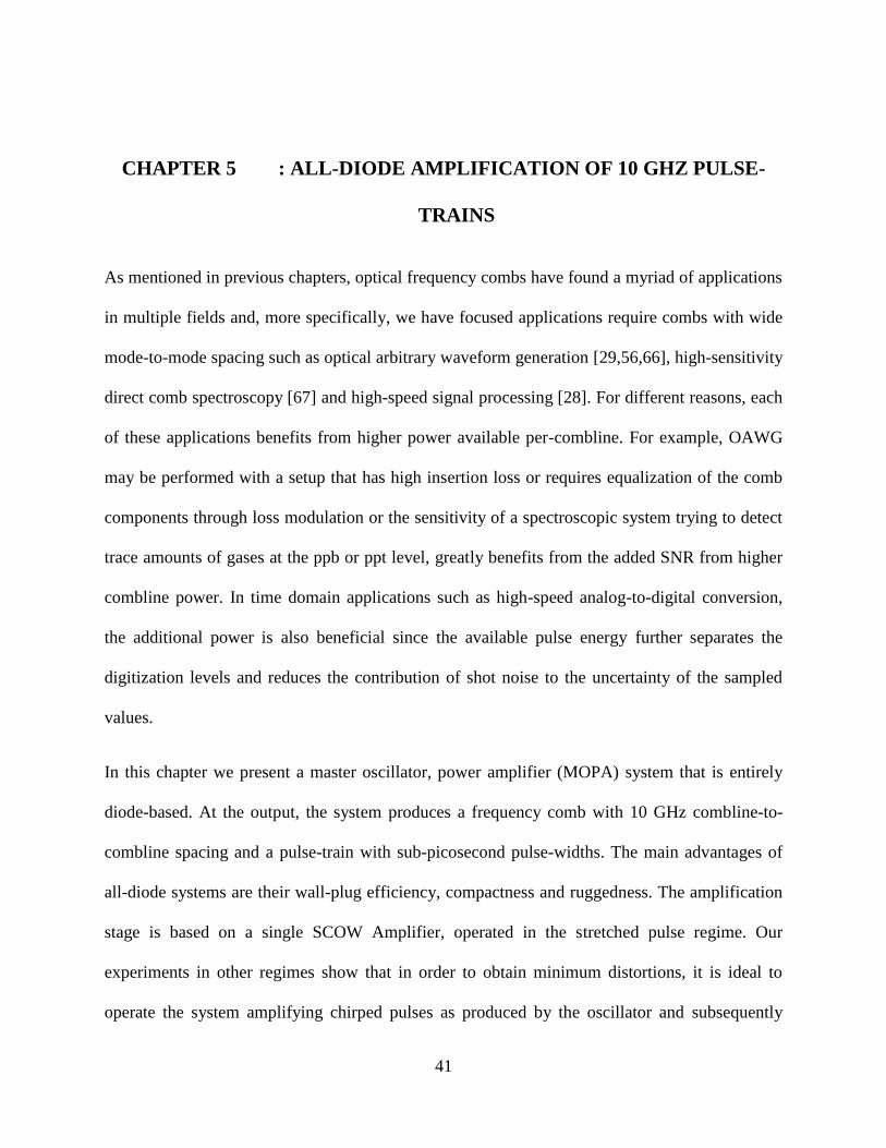
41
CHAPTER 5 : ALL-DIODE AMPLIFICATION OF 10 GHZ PULSE-
TRAINS
As mentioned in previous chapters, optical frequency combs have found a myriad of applications
in multiple fields and, more specifically, we have focused applications require combs with wide
mode-to-mode spacing such as optical arbitrary waveform generation [29,56,66], high-sensitivity
direct comb spectroscopy [67] and high-speed signal processing [28]. For different reasons, each
of these applications benefits from higher power available per-combline. For example, OAWG
may be performed with a setup that has high insertion loss or requires equalization of the comb
components through loss modulation or the sensitivity of a spectroscopic system trying to detect
trace amounts of gases at the ppb or ppt level, greatly benefits from the added SNR from higher
combline power. In time domain applications such as high-speed analog-to-digital conversion,
the additional power is also beneficial since the available pulse energy further separates the
digitization levels and reduces the contribution of shot noise to the uncertainty of the sampled
values.
In this chapter we present a master oscillator, power amplifier (MOPA) system that is entirely
diode-based. At the output, the system produces a frequency comb with 10 GHz combline-to-
combline spacing and a pulse-train with sub-picosecond pulse-widths. The main advantages of
all-diode systems are their wall-plug efficiency, compactness and ruggedness. The amplification
stage is based on a single SCOW Amplifier, operated in the stretched pulse regime. Our
experiments in other regimes show that in order to obtain minimum distortions, it is ideal to
operate the system amplifying chirped pulses as produced by the oscillator and subsequently

42
compress in a posterior stage. Spectral and temporal domain analysis of the pulse distortions is
presented as well as noise characterization of the original and amplified pulse-trains.
1.Overall MOPA system
The Master Oscillator is kept as described on Chapter 4, including stabilization loops and intra-
cavity dispersion compensation and a low noise Sapphire-Loaded Crystal Oscillator is used for
mode-locking. The amplification stage consists of a SCOWA with lower gain and higher
saturation power than the laser chip. Gain measurements with cw light input were performed and
the small signal gain at 4 A of bias current is 15 dB and saturation power is ~25 dBm. The
complete system is depicted in Figure 5.1. The output of the oscillator is isolated from possible
reflections from connectors as well as amplified spontaneous emission from the power amplifier
by placing a Faraday isolator at its output. One-tenth of the laser output is used for diagnostics,
which include optical spectrum analysis, photodetection followed by RF spectral analysis and a
sampling oscilloscope. The set of diagnostics connections are shown in the dashed box in Figure
5.1 and are kept as a unit and used for either the original pulse-train or the amplified pulse-train.
After amplification, only one-hundredth of the output is used for the standard diagnostics and the
power used in residual phase noise measurements is carefully controlled to match the power used
when the same measurement is performed on the pulse-train directly from the oscillator. A
dispersion stage consisting of an optimized length of SMF (depicted as D in Figure 5.1) is used
to compress the pulses either before or after the amplifier.
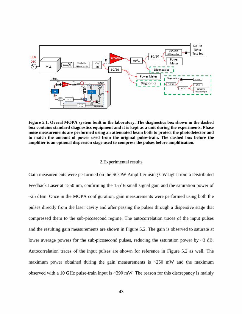
43
Figure 5.1. Overal MOPA system built in the laboratory. The diagnostics box shown in the dashed
box contains standard diagnostics equipment and it is kept as a unit during the experiments. Phase
noise measurements are performed using an attenuated beam both to protect the photodetector and
to match the amount of power used from the original pulse-train. The dashed box before the
amplifier is an optional dispersion stage used to compress the pulses before amplification.
2.Experimental results
Gain measurements were performed on the SCOW Amplifier using CW light from a Distributed
Feedback Laser at 1550 nm, confirming the 15 dB small signal gain and the saturation power of
~25 dBm. Once in the MOPA configuration, gain measurements were performed using both the
pulses directly from the laser cavity and after passing the pulses through a dispersive stage that
compressed them to the sub-picosecond regime. The autocorrelation traces of the input pulses
and the resulting gain measurements are shown in Figure 5.2. The gain is observed to saturate at
lower average powers for the sub-picosecond pulses, reducing the saturation power by ~3 dB.
Autocorrelation traces of the input pulses are shown for reference in Figure 5.2 as well. The
maximum power obtained during the gain measurements is ~250 mW and the maximum
observed with a 10 GHz pulse-train input is ~390 mW. The reason for this discrepancy is mainly

44
due to the multiple diagnostics taps used to carefully calibrate the gain measurements, which
limits the amount of power available for the amplification stage.
Figure 5.2. Gain measurements with pulses directly from the cavity and after compression. On the
left side, autocorrelation traces of the pulses input to the amplification stage. On the right side a
plot of Gain vs. Output power for the long (short) pulses in black (red).
From the gain measurements, it can be concluded that the amplifier is operating in a nonlinear
regime when illuminated with short pulses; therefore the manifestation of spectral distortions is
expected. To confirm this, optical spectra were recorded at different input powers to the
amplifier. Figure 5.3 shows these measurements for amplification of long and short pulses. In the
case of long pulses only a small red-shift is observed as the power is increased. This can be
attributed to the fact that the pulses are up-chirped and therefore the red edge for the pulse sees a
slightly higher gain as it passes through the amplifier. In the case of short pulses, much larger
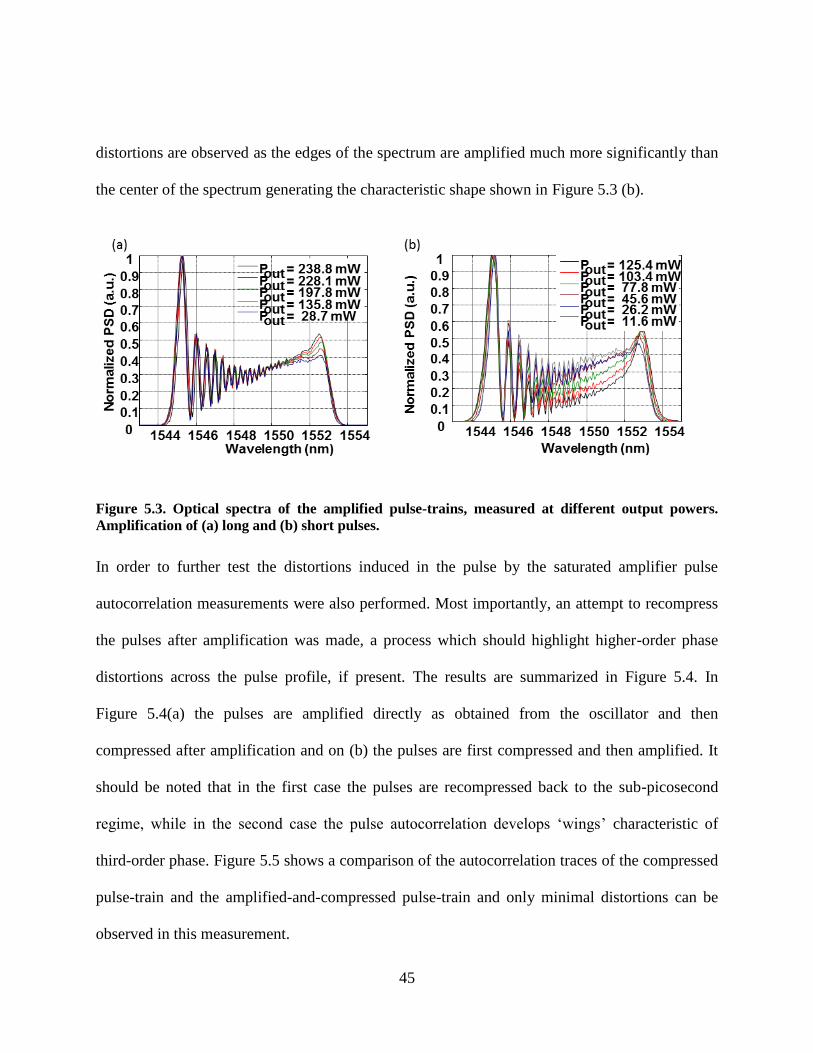
45
distortions are observed as the edges of the spectrum are amplified much more significantly than
the center of the spectrum generating the characteristic shape shown in Figure 5.3 (b).
Figure 5.3. Optical spectra of the amplified pulse-trains, measured at different output powers.
Amplification of (a) long and (b) short pulses.
In order to further test the distortions induced in the pulse by the saturated amplifier pulse
autocorrelation measurements were also performed. Most importantly, an attempt to recompress
the pulses after amplification was made, a process which should highlight higher-order phase
distortions across the pulse profile, if present. The results are summarized in Figure 5.4. In
Figure 5.4(a) the pulses are amplified directly as obtained from the oscillator and then
compressed after amplification and on (b) the pulses are first compressed and then amplified. It
should be noted that in the first case the pulses are recompressed back to the sub-picosecond
regime, while in the second case the pulse autocorrelation develops ‘wings’ characteristic of
third-order phase. Figure 5.5 shows a comparison of the autocorrelation traces of the compressed
pulse-train and the amplified-and-compressed pulse-train and only minimal distortions can be
observed in this measurement.

46
Figure 5.4. Pulse autocorrelation traces before and after amplification. (a) Amplifying pulses
directly from the oscillator and subsequently compressing and (b) amplifying compressed pulses.
Figure 5.5. Comparison of compressed pulse autocorrelations before (red) and after (blue)
amplification.

47
Finally, residual noise measurements were also performed on the amplified pulse-trains to
quantify the noise added by the amplification stage. The results are shown in Figure 5.6 and as
can be observed, no additional noise can be measured at the current stage. The technical noise is
faithfully amplified together with the signal while the shot noise level is kept equal by placing
equal amounts of average optical power on the photodetector.
Figure 5.6 (a) Phase and (b) amplitude noise measurements for the pulse-trains before (black) and
after (red) amplification
3.Conclusions
In conclusion, we have demonstrated a master oscillator and power amplifier system based
entirely on diode amplifiers which produces >250 mW of average optical power (maximum
observed 390 mW) in a 10 GHz optical frequency comb. The amplification can be performed
with minimal distortions if the amplification stage is fed with chirped pulses as produced by the
oscillator and the output of the amplification stage has been compressed to the sub-picosecond
48
regime. These systems can potentially find applications on optics-assisted sampling for analog to
digital converters, optical arbitrary waveform generation and multi-heterodyne spectroscopy to
name a few.
49
CHAPTER 6 : FREQUENCY STABILITY OF A MODE-LOCKED
LASER WITH A 10,000 FINESSE FABRY-PEROT ETALON
The central element in the type of comb sources presented in this dissertation (as well as in
refs. [35,50]) is the inclusion of a high-finesse optical cavity, coupled to a long fiber ring cavity.
The reason behind the inclusion of such high-finesse filter is the suppression of the interleaved
cavity modes to accomplish a laser that operates as a comb source at 10 GHz. Besides this, the
Fabry-Pérot Etalon (FPE) accomplishes at least three more purposes inside the cavity. The first
one is the elimination of the so-called supermode noise spurs, which present themselves as noise
that is periodic with the fundamental frequency of the cavity a known detrimental effect of
harmonic mode-locking. The second effect is that this cavity is able to filter out broadband
spontaneous emission from the gain medium and the last one is that the FPE becomes a
frequency reference for the comb-lines. In this chapter, a new laser system using a 10,000
Finesse etalon is constructed and characterized. This FPE is held in a vacuum chamber whose
temperature is controlled in order to achieve an improvement on the absolute frequency stability
of the comb. Also, an attempt is made at measuring the suppression of out-of-band ASE by
placing several output couplers around the optical cavity and making spectral measurements with
both a system with a 1,000 Finesse etalon and a 10,000 Finesse etalons.
1.Experimental setup
The experimental setup of the laser used in this chapter is shown in Figure 6.1 and it is very
similar to previous implementations of the system, so details about the general laser architecture
50
are omitted in this chapter and the reader is referred to previous chapters and refs. [35,50] where
details about the operation and performance of previously demonstrated sources can be found. In
brief, the laser is mode-locked via loss modulation by driving the intensity modulator (IM) at a
rate equal to the free-spectral range (FSR) of the FPE. The cavity length is actively stabilized by
using a multi-combline Pound-Drever-Hall (PDH) stabilization scheme, shown in the dashed box
in Figure 6.1. Note that multiple taps have been placed around the cavity which are used to
characterize the evolution of the pulses as they travel around the cavity. The optical cavity is
comprised mostly of single mode fiber (~20m) and a short section of dispersion compensating
fiber (~2m), yielding a ~9 MHz cavity, which is then mode-locked at a harmonic close to the
~1,130th, to closely match the FSR of the FPE. Contrary to previous experience, it was found
that it was quite challenging to mode-lock the laser before the dispersion compensation was in
place. We currently attribute this to a walk-off between the cold fiber cavity modes and the
modes of the FPE.

51
Figure 6.1. Schematic of the mode-locked laser utilized in this experiment. CIR: Circulator, DBM:
Double Balanced Mixer, DCF: Dispersion Compensating Fiber, FPE: Fabry-Pérot Etalon, IM:
Intensity Modulator, ISO: isolator, OC: output coupler, PC: Polarization controller, PD:
Photodetector, PBS: Polarizing Beam Splitter, PM: Electro-optic Phase Modulator, PZT:
Piezoelectric Fiber Stretcher, SOA: Semiconductor Optical Amplifier, VOD: Variable Optical
Delay. The PBS used to multiplex the error signal is a bulk component. The FPE is kept in a
vacuum and temperature stabilized enclosure.
2. Experimental results
Characterization data of the laser is shown in Figure 6.2. Figure 6.2 (a) shows two optical
spectra taken from the port B, immediately after the SOA (red line) and from port C, after the
light has passed through the FPE (black line). It is evident from the plot that background ASE is
significantly filtered by the cavity. In the plot shown ASE is suppressed to below the noise-floor
of the instrument. Further measurements were performed and are compared to a mode-locked
laser with a 1,000 Finesse etalon in the next section. Figure 6.2 (b) shows two autocorrelation
traces after the pulses have been passed through 20 m and 90 m of SMF. The smooth curve
(blue) is a calculation of the transform-limited autocorrelation using the measured optical
spectrum. The full-width at half-maximum (FWHM) of the measured autocorrelation after 90 m
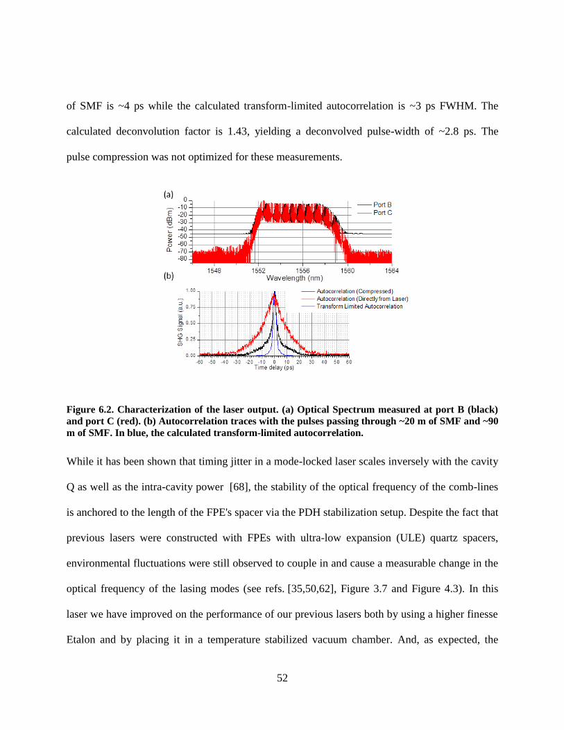
52
of SMF is ~4 ps while the calculated transform-limited autocorrelation is ~3 ps FWHM. The
calculated deconvolution factor is 1.43, yielding a deconvolved pulse-width of ~2.8 ps. The
pulse compression was not optimized for these measurements.
Figure 6.2. Characterization of the laser output. (a) Optical Spectrum measured at port B (black)
and port C (red). (b) Autocorrelation traces with the pulses passing through ~20 m of SMF and ~90
m of SMF. In blue, the calculated transform-limited autocorrelation.
While it has been shown that timing jitter in a mode-locked laser scales inversely with the cavity
Q as well as the intra-cavity power [68], the stability of the optical frequency of the comb-lines
is anchored to the length of the FPE's spacer via the PDH stabilization setup. Despite the fact that
previous lasers were constructed with FPEs with ultra-low expansion (ULE) quartz spacers,
environmental fluctuations were still observed to couple in and cause a measurable change in the
optical frequency of the lasing modes (see refs. [35,50,62], Figure 3.7 and Figure 4.3). In this
laser we have improved on the performance of our previous lasers both by using a higher finesse
Etalon and by placing it in a temperature stabilized vacuum chamber. And, as expected, the

53
obtained comb is much more robust against environmental fluctuations. In previous
measurements, we were also limited by the fact that the laser used for the comparison was free-
running [50,62]. To improve our measurement method, we have used a fully stabilized frequency
comb as reference. The experimental setup for the measurement is shown in Figure 6.3. The
reference comb is a commercially-available (Menlo Systems), fiber-based mode-locked laser in
which both frep and fceo are stabilized to a microwave reference. The repetition rates are detuned
from an exact harmonic in order to generate a multi-heterodyne spectrum, which is subsequently
filtered and analyzed in a real-time spectrum analyzer. The only drawback of this setup is that
the reference comb has a relatively broad comb line-width, in the order of 100 kHz.
Figure 6.3. Multi-heterodyne experimental setup. RT-RFSA: real time Spectrum Analyzer.
The beating of two frequency combs produces a multi-heterodyne spectrum, which allows us to
track the frequency of multiple (14 in this case, but this is not limited by the method) beat-notes
simultaneously using a real-time radiofrequency spectrum analyzer to record the spectrogram
which is then analyzed for frequency deviations. The repetition rate of the reference source is
stabilized to 250.955 MHz and the source under test is mode-locked at the FSR of the FPE,
10.2898 GHz. Therefore, the effective repetition rate detuning
kHz.
A single trace of such multi-heterodyne spectrum is shown in Figure 6.4. These spectra were
continuously recorded for ~6 min on one measurement day (Dec/13/2012) and for ~12 min the
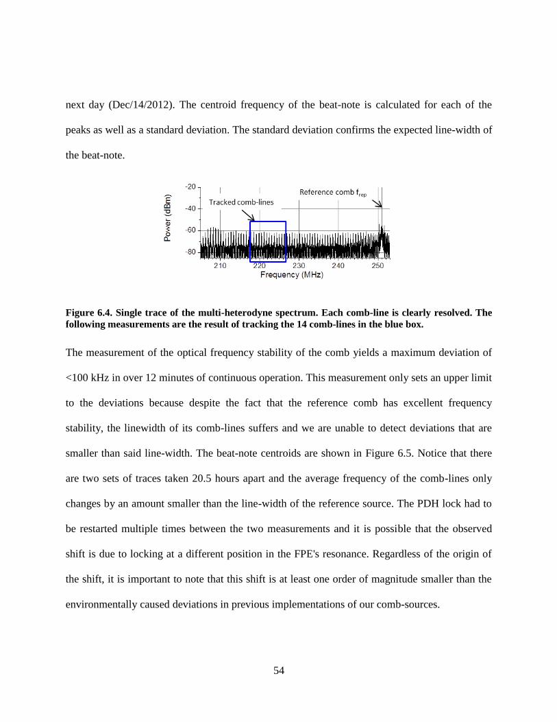
54
next day (Dec/14/2012). The centroid frequency of the beat-note is calculated for each of the
peaks as well as a standard deviation. The standard deviation confirms the expected line-width of
the beat-note.
Figure 6.4. Single trace of the multi-heterodyne spectrum. Each comb-line is clearly resolved. The
following measurements are the result of tracking the 14 comb-lines in the blue box.
The measurement of the optical frequency stability of the comb yields a maximum deviation of
<100 kHz in over 12 minutes of continuous operation. This measurement only sets an upper limit
to the deviations because despite the fact that the reference comb has excellent frequency
stability, the linewidth of its comb-lines suffers and we are unable to detect deviations that are
smaller than said line-width. The beat-note centroids are shown in Figure 6.5. Notice that there
are two sets of traces taken 20.5 hours apart and the average frequency of the comb-lines only
changes by an amount smaller than the line-width of the reference source. The PDH lock had to
be restarted multiple times between the two measurements and it is possible that the observed
shift is due to locking at a different position in the FPE's resonance. Regardless of the origin of
the shift, it is important to note that this shift is at least one order of magnitude smaller than the
environmentally caused deviations in previous implementations of our comb-sources.
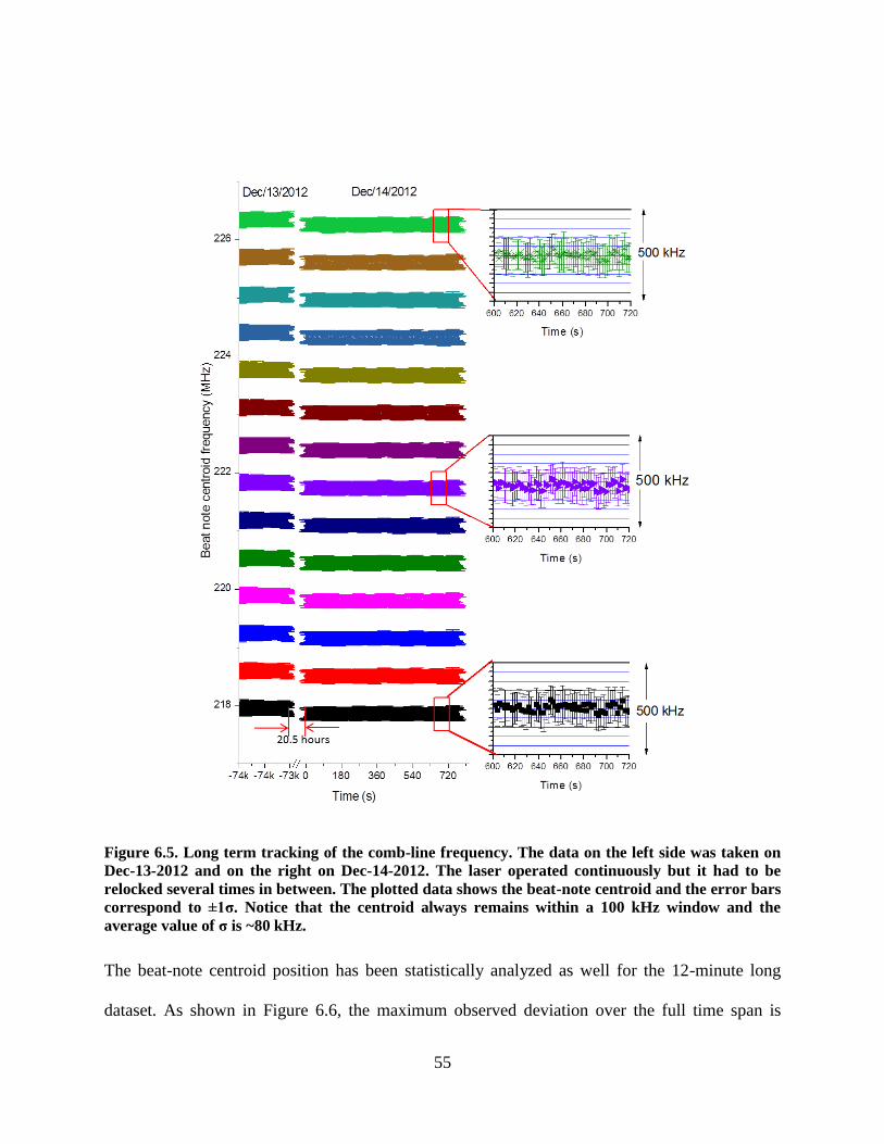
55
Figure 6.5. Long term tracking of the comb-line frequency. The data on the left side was taken on
Dec-13-2012 and on the right on Dec-14-2012. The laser operated continuously but it had to be
relocked several times in between. The plotted data shows the beat-note centroid and the error bars
correspond to ±1σ. Notice that the centroid always remains within a 100 kHz window and the
average value of σ is ~80 kHz.
The beat-note centroid position has been statistically analyzed as well for the 12-minute long
dataset. As shown in Figure 6.6, the maximum observed deviation over the full time span is

56
always under 100 kHz (< 90 kHz, with the exception of an anomalous data-point in the second
beat-note) and twice the standard deviation is <40 kHz.
Figure 6.6. Statistics of the beat-note centroid positions. 2xσ is plotted in black squares and the
maximum observed deviation over 12 minutes in red circles. Notice that even the maximum
observed deviations are within one beat-note line-width.
3. Amplified spontaneous emission suppression as a function of filter Finesse
Another one of the functionalities that the FPE performs in the cavity is the suppression of
broadband amplified spontaneous emission from the amplifier. A simple mathematical analysis
of the transfer function of the FPE shows that the expected suppression is inversely proportional
to the Finesse of the FPE. Measurements of this suppression were performed on a mode-locked
laser with a 1,000 Finesse etalon and then with a 10,000 Finesse etalon by recording the optical
spectra in a coupler before and after the FPE. The fiber cavities contained the exact same
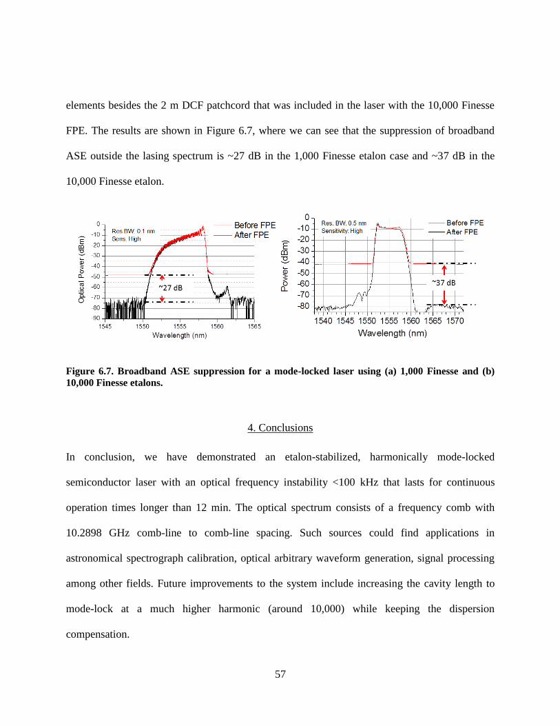
57
elements besides the 2 m DCF patchcord that was included in the laser with the 10,000 Finesse
FPE. The results are shown in Figure 6.7, where we can see that the suppression of broadband
ASE outside the lasing spectrum is ~27 dB in the 1,000 Finesse etalon case and ~37 dB in the
10,000 Finesse etalon.
Figure 6.7. Broadband ASE suppression for a mode-locked laser using (a) 1,000 Finesse and (b)
10,000 Finesse etalons.
4. Conclusions
In conclusion, we have demonstrated an etalon-stabilized, harmonically mode-locked
semiconductor laser with an optical frequency instability <100 kHz that lasts for continuous
operation times longer than 12 min. The optical spectrum consists of a frequency comb with
10.2898 GHz comb-line to comb-line spacing. Such sources could find applications in
astronomical spectrograph calibration, optical arbitrary waveform generation, signal processing
among other fields. Future improvements to the system include increasing the cavity length to
mode-lock at a much higher harmonic (around 10,000) while keeping the dispersion
compensation.

58
CHAPTER 7 : APPLICATION OF FREQUENCY COMBS IN MULTI-
HETERODYNE MEASUREMENTS. PART I: THEORY
Since its invention, the optical frequency comb [1,3,69], has been applied to several fields such
as time and frequency metrology [4,70,71], length metrology [20], optical arbitrary waveform
generation [27,28,56,66,72,73], and high precision spectroscopy [23]. All of these applications
benefit from the fact that the frequency comb consists of a large set of coherent local oscillators
with uniform frequency spacing. These oscillators can then probe the resonances of a molecular
or atomic system in spectroscopic measurements, and become the Fourier basis whose
amplitudes and phases are controlled for arbitrary waveform generation or provide the link
between the optical frequency of a single combline and the microwave frequencies represented
by the combline spacing in optical clocks.
Sampling electric fields directly at optical frequencies is practically an impossible task given the
fact that the center frequency of the oscillation is well beyond the capabilities of electronic
sampling devices. Notwithstanding, most optical signals contain information only within a small
bandwidth (i.e., they are bandlimited). Heterodyning a high-frequency but bandlimited signal
with a coherent oscillator produces an exact copy of the bandlimited signal centered at a
frequency corresponding to the frequency difference between the coherent oscillator and the
signal under test. This low-frequency copy can then be sampled by electronic means. This
principle can be applied to optical signals, that is, a narrowband optical signal can be
heterodyned with a continuous wave (CW) laser and sampled at the beat frequency. If the signal
59
is distributed over periodically spaced portions of spectrum, it can be heterodyned with a set of
coherent oscillators with different frequency spacing to generate a series of beat notes in the RF
domain that can then be sampled. Heterodyne techniques are useful because both amplitude and
phase information are retained in the process. Some of the requirements for the local oscillators
are frequency stability and a fixed phase relation between them, both of which are typically met
by frequency comb sources.
Multiheterodyne detection with optical frequency combs was first proposed in [22] and has been
implemented in a coherent configuration where two combs that share an optical reference are
mixed and from the mixing products the effect of a medium on the signal comb can be
deduced [23,74,75]. The mutual coherence of these combs makes possible the accumulation of
signal over extended periods of time, beyond the coherence time of individual comblines.
In our experiments, we utilize a frequency comb as a set of local oscillators to downconvert and
sample periodic optical signals. The optical signals that are being sampled are not coherent with
the local oscillator, which is a realistic approximation to measuring unknown optical signals as is
the case in the spectral characterization of rapidly tunable CW lasers [76], mode-locked laser
systems, and arbitrarily shaped optical waveforms. The most evident limitations are that the
waveforms must have an underlying periodicity and that the lack of mutual coherence sets a limit
on the maximum time over which signal can be accumulated. Three types of experiments are
presented, wherein different types of sources are sampled: 1) pulses from an independent optical
frequency comb source; 2) phase-modulated, CW light; and 3) periodically filtered, incoherent
white light. In the first two experiments, the repetition rates are extremely detuned, by more than
60
a multiple of the repetition rate of the lower repetition rate source and, therefore, the
downconversion is performed using only a subset of the available comblines. An effective
repetition rate detuning is introduced to accurately describe these experiments. In the third case,
photocurrent interferometry of signals detected with time delays between them is performed to
demonstrate the fidelity of the measurement.
This chapter is organized as follows. In the next section a conceptual description of the
experiments is presented by considering the sources to have infinitely narrow (represented by
Dirac delta functions) frequency components. Following this section, a more rigorous treatment
of the signals is presented and the analysis extended to random signals with bandlimited spectral
content. The experimental results are left for the next chapter where our experiments will be
described in detail.
1.Conceptual description
Equivalent time and frequency domain pictures can be drawn to explain the phenomena at hand.
A conceptual form of the experimental setup is shown in Fig. 1, where one of the sources is an
optical frequency comb and the other is the source under test. For this description, we shall
assume that the source under test is a frequency comb with narrow components whose
amplitudes and phases are unknown. This assumption is valid as long as the observation time
does not exceed the coherence time, which can be on the order of hundreds of microseconds to
milliseconds for free-running, narrow-linewidth lasers [50], while cavity stabilized lasers have
reached the sub-hertz linewidth regime [77–79], allowing for second-long observation times.
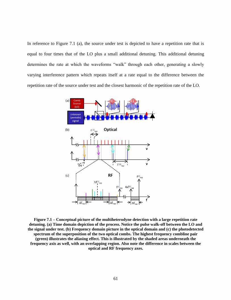
61
In reference to Figure 7.1 (a), the source under test is depicted to have a repetition rate that is
equal to four times that of the LO plus a small additional detuning. This additional detuning
determines the rate at which the waveforms “walk” through each other, generating a slowly
varying interference pattern which repeats itself at a rate equal to the difference between the
repetition rate of the source under test and the closest harmonic of the repetition rate of the LO.
Figure 7.1 – Conceptual picture of the multiheterodyne detection with a large repetition rate
detuning. (a) Time domain depiction of the process. Notice the pulse walk-off between the LO and
the signal under test. (b) Frequency domain picture in the optical domain and (c) the photodetected
spectrum of the superposition of the two optical combs. The highest frequency combline pair
(green) illustrates the aliasing effect. This is illustrated by the shaded areas underneath the
frequency axis as well, with an overlapping region. Also note the difference in scales between the
optical and RF frequency axes.
62
From the frequency domain picture [see Figure 7.1 (b) and (c)], it can be readily seen that the RF
beat notes will appear at the frequency difference between each pair of comblines. The effective
repetition rate detuning determines the rate at which the comblines from each source walk-off
from each other, thus determining the beat-note spacing in the RF domain. It should be noted that
for large detuning or a large interacting bandwidth, the beat notes may get to the point where the
next closest combline is not to the lower frequency side but to the higher frequency side. When
this occurs, a different set of beat notes with the same spacing but at an overall offset will appear
within the region of interest, generating a signal with a slower overall periodicity (aliased). To
avoid this problem the following limit must be satisfied:
| |
( )
( 7.1 )
In this expression, N is the number of interacting comblines,
( ) (
( ) ( )
⁄ ) ( )
is the effective repetition rate detuning, ( )
is the
larger of the two repetition rates, and is the frequency difference between the two closest
comblines. From ( 7.1 ), we can see that there is a tradeoff between the maximum repetition rate
detuning and the available interacting bandwidth. The frequency difference of the two closest
comblines also affects the maximum usable bandwidth and, in some cases, it can be tuned to a
convenient value by changing the carrier-envelope offset frequency of the reference comb. For
example, assume ( ) and
( ) , then ⌊
( ) ( )
⁄ ⌋ and the beat-note
spacing . A maximum of 50 beat notes can be
63
observed within the band from dc to ( )
⁄ , which limits the optical bandwidth that
can be used before aliasing effects appear to a maximum of 200 GHz.
The equivalent time domain picture is that of a sampling gate that has variable delay with respect
to the periodic signal under test, given by the pulse walk-off. The relative position of the
pulses/waveforms comes back to its original position after a time equal to ⁄ , which in turn
gives rise to the beat-note spacing in the RF domain.
It is important to note that this is a linear technique and, consequently, the interacting quantities
are the electric fields. The resulting waveforms arise from electric field interference, which, if
the local oscillator is properly characterized, gives a snapshot of the periodic signal under test,
including the carrier under the envelope.
This process achieves two independent forms of spectral conversion: 1) it downconverts the
carrier frequency from the optical domain to the RF domain; and 2) it compresses the spectrum
by reducing the “empty” spaces in between comblines from the original repetition rate to the new
sampled rate, given by the repetition rate detuning. The downconversion factor can be defined as
the carrier optical frequency divided by the carrier microwave frequency and the compression
factor as the ratio of the original repetition rate to the sampled repetition rate.
As the repetition rate detuning is reduced, the generated waveforms have a longer periodicity.
This detuning must evidently reach a point where the periodicity is longer than the coherence of
the sources. In the frequency domain, this can be thought of as an overlap between finite-
linewidth components (as opposed to the ideal delta-like components described so far) when the
64
spectral compression is carried beyond the linewidth of individual comblines. A more detailed
analysis of the signals obtained from finite linewidth signals is presented in the next section, but
it must be stated that a lower limit to the repetition rate detuning can be written as:
( 7.2 )
where ΔνLW is a parameter that represents the linewidth of the individual comblines and its
definition may vary depending on the particular application.
2.Heterodyne detection of bandlimited white light and periodically filtered white light
When the source under test is a bandlimited white light source, the corresponding electric fields
can be represented through a Fourier expansion whose frequency component pacing depends
inversely on the observation time. A classical analysis for the correlations between two delayed
copies of a white light signal is developed by Hanbury Brown and Twiss [80]. In this paper, a
heterodyne version of the derivation is presented for a single combline and the conclusions can
be extended to the multi-combline beating by superposing individual solutions as long as the
condition in ( 7.2 ) is fulfilled.
An advantage of using heterodyne detection to downconvert a white light spectrum is that the
resulting photocurrent interferometry has extremely high resolution, limited only by the available
RF spectrum analyzers. As a comparison, a typical grating based optical spectrum analyzer can
resolve fringes with a resolution on the order of 1 GHz, while a RF spectrum analyzer could
65
potentially resolve spectral fringes with spacing smaller than 1 Hz. The power spectral density of
the white light spectrum then becomes the ultimate limitation in the detectability of the fringes.
A few assumptions must be stated first: 1) The white light is considered band-limited; 2) the
local oscillator is assumed to be coherent (i.e., a delta-like function); and 3) the frequency
difference between the local oscillator and the closest nonzero frequency component of the white
light is larger than the white light bandwidth. This allows us to treat the white light homodyne
beats independently from the heterodyne beats. The assumptions are not extremely constraining,
provided careful filtering.
A random but bandlimited optical field is considered in this derivation. In general, the spectrum
of a bandlimited signal may consist of a finite number of sparsely located finite bandwidth peaks.
If such a random electric field is observed for a finite time τ, then it can be represented by a
Fourier series in the following form:
( ) ∑ | | [
]
( 7.3 )
where the coefficients qn are related to the integrated optical power in the nth frequency bin and
are nonzero only for a finite frequency range,
. are the phases of the
frequency components and are assumed to be uniformly distributed over the range [0,2]. As
shown in the analysis in [80], the photocurrent generated by such a field is given by
( ) ⟨ ⟩ ∑ √ √ [
( ) ( )]
( 7.4 )

66
where is the photodetector responsivity, ⟨ ⟩ is the average power contained in the signal
and Pn and Pm are the average powers contained in the nth and mth frequency bins, respectively.
The photocurrent fluctuations represented by the second term in ( 7.4 ) average zero, but,
nonetheless, they can be shown to be correlated to the signals detected at a time delay . The
case that is of interest to us in this work is a heterodyne version of this experiment. The total
electric field obtained by adding a CW carrier to a random signal like the one in ( 7.3 ) is given
by:
( ) [ ] ∑ [
]
( 7.5 )
The photodetected signal has four main components: the two terms in ( 7.4 ) plus an additional
average power due to the local oscillator and a heterodyne term. As long as care is taken to keep
the frequency difference between the local oscillator and the center of the white light’s spectrum
larger than the white light bandwidth, the heterodyne term can be filtered and observed
independently in the RF domain. The voltage across a resistor RL of the heterodyne part of the
photodetected signal is given by
( )( ) √ ∑√ [ (
) ( )]
( 7.6 )

67
Figure 7.2 – Conceptual experimental setup for white light photocurrent interferometry.
After including delays at different positions (see Fig. 9) at the second photodetector, the voltage
is
( )( ) √ ∑√ [ (
) ( )
]
( 7.7 )
Note that phase delays in the optical paths ( and ) change the phase of the photodetected
spectrum directly. If we add the signals ( ) and ( ) in an RF coupler as shown in Figure 7.2,
the interference pattern will have a fringe spacing related to the accumulated delay between the
white light paths, but the fringe position will be extremely sensitive to small path changes in the
order of the wavelength of light, due to the phase factor (
). The expression
for the spectral interference is given by:
| {
( ( )( ) ( )( ))}| [ (
)
]
( ) (
)
( 7.8 )
where ( ) ( ⁄ ) is the Fourier transform of the signal in a single channel. Notice that ⁄
and are optical frequencies. As a consequence, while the periodicity of the interference pattern
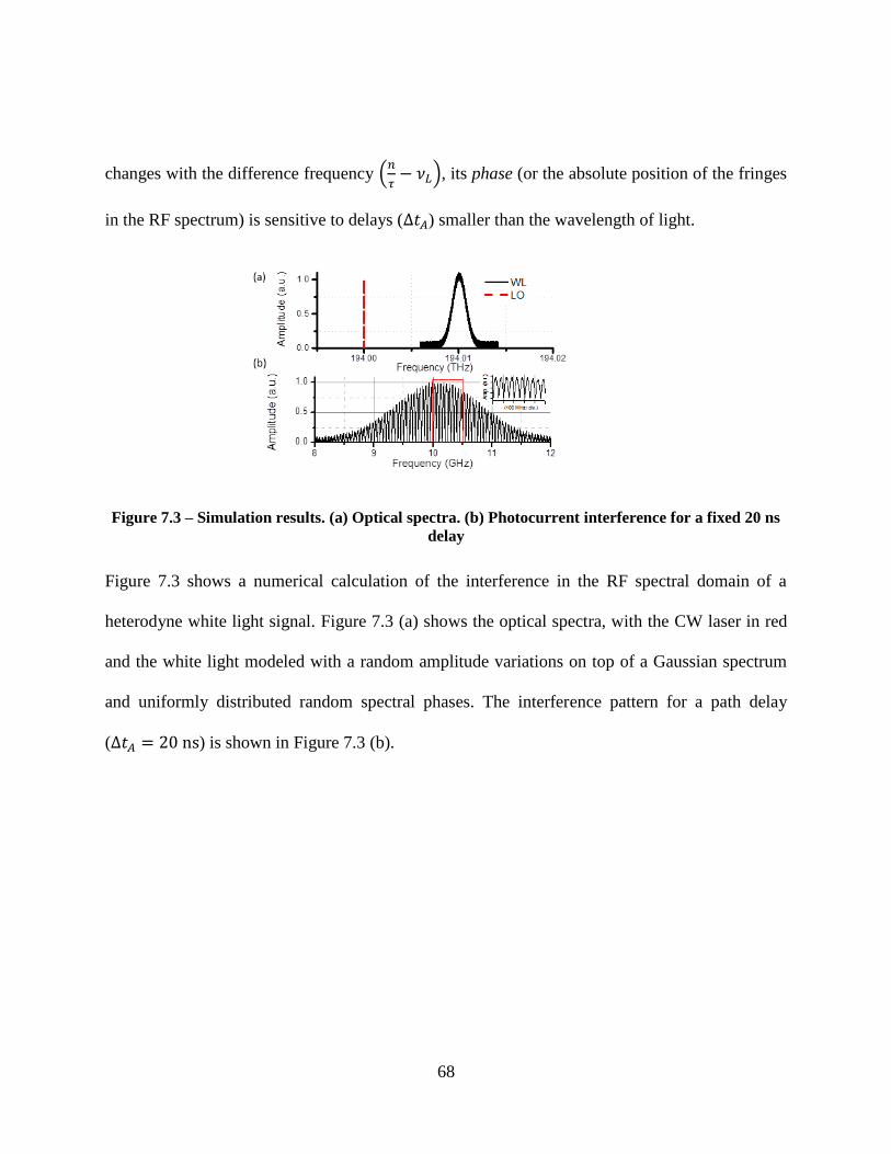
68
changes with the difference frequency (
), its phase (or the absolute position of the fringes
in the RF spectrum) is sensitive to delays ( ) smaller than the wavelength of light.
Figure 7.3 – Simulation results. (a) Optical spectra. (b) Photocurrent interference for a fixed 20 ns
delay
Figure 7.3 shows a numerical calculation of the interference in the RF spectral domain of a
heterodyne white light signal. Figure 7.3 (a) shows the optical spectra, with the CW laser in red
and the white light modeled with a random amplitude variations on top of a Gaussian spectrum
and uniformly distributed random spectral phases. The interference pattern for a path delay
( ) is shown in Figure 7.3 (b).
69
CHAPTER 8 : APPLICATION OF FREQUENCY COMBS IN MULTI-
HETERODYNE MEASUREMENTS. PART II: EXPERIMENTAL
RESULTS
The experiments presented cover various cases for which multiheterodyning an unknown,
periodic, optical signal with a frequency comb is useful as a means to downconvert and sample
the electric fields. Although all the experiments are conceptually very similar, in practice, they
represent a broad set of cases. For this reason, the metrics for evaluation of the performance of
the experimental setups are chosen specifically for each of the experiments. In some cases, the
availability of different diagnostic tools also determines the type of analysis that can be
performed.
This chapter is organized as follows: the first section deals with pairs of optical frequency comb
sources generated from mode-locked lasers, the second section deals with a mode-locked laser
comb which samples phase modulated continuous wave light and the third section includes
experiments done with periodically filtered white light.
1.Mode-locked pulses
In the first experiment, an erbium-doped fiber passively mode-locked laser source is used as a
local oscillator to sample the electric field from a semiconductor-based harmonically mode-
locked laser, locked to an intracavity Fabry–Pérot etalon (FPE) [35]. The repetition rates of the

70
lasers are ~250 MHz and ~10.24 GHz, respectively. The detuning is extremely large and only the
beat notes from the 250 MHz spaced comblines that are nearest to the 10 GHz spaced comblines
are used in the measurement, yielding an effective repetition rate detuning of ~600 kHz, which is
calculated by comparing the 41st harmonic of the fiber laser with the fundamental of the 10.24
GHz comb source. This is equivalent to sampling one out of every forty-one 10.24 GHz
repetition rate pulses on each cycle.
Optical and RF spectra of the results are shown in Figure 8.1. An effort was made in this
experiment to make the detuning large enough to almost fill the available RF bandwidth (1/2 of
250 MHz) for one copy of the spectrum. The absolute position of the downconverted comb can
also be controlled by varying the carrier-envelope offset frequency of the 250 MHz comb. A
smaller span of the RF measurement shows clearly resolved beat notes in Figure 8.1 (c). The
interacting bandwidth is essentially the optical bandwidth of the semiconductor mode-locked
laser which is ~2.12 THz, that is, more than 200 comblines. The downconversion factor
( ⁄ ) is on the order of , and the compression factor ( ⁄ ) is .

71
Figure 8.1 – (a) Optical spectra of the mode-locked comb sources. (b) Photodetected RF spectrum.
(c) Smaller span of the RF spectrum.
In order to test whether the spectral phase information is preserved, the photodetected signal is
low pass filtered (ideally with a filter that cuts off everything above 125 MHz, but in this case,
the oscilloscope bandwidth was limited to 80 MHz) and the resulting waveform is sampled with
an electrical oscilloscope. The semiconductor laser’s pulses are then passed through different
amounts of dispersion (~100 m of standard single-mode fiber with ( ⁄ ) and a
few meters of dispersion compensating fiber with ( ⁄ )). The results are
shown in Figure 8.2, where it can be observed that as the pulse chirp, and hence, the spectral
phase of the optical signal is varied, the chirp and pulse duration of the RF signal varies
accordingly.
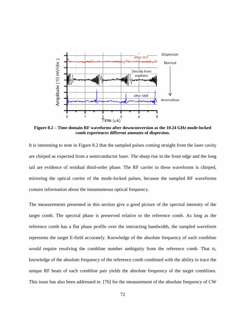
72
Figure 8.2 – Time domain RF waveforms after downconversion as the 10.24 GHz mode-locked
comb experiences different amounts of dispersion.
It is interesting to note in Figure 8.2 that the sampled pulses coming straight from the laser cavity
are chirped as expected from a semiconductor laser. The sharp rise in the front edge and the long
tail are evidence of residual third-order phase. The RF carrier in these waveforms is chirped,
mirroring the optical carrier of the mode-locked pulses, because the sampled RF waveforms
contain information about the instantaneous optical frequency.
The measurements presented in this section give a good picture of the spectral intensity of the
target comb. The spectral phase is preserved relative to the reference comb. As long as the
reference comb has a flat phase profile over the interacting bandwidth, the sampled waveform
represents the target E-field accurately. Knowledge of the absolute frequency of each combline
would require resolving the combline number ambiguity from the reference comb. That is,
knowledge of the absolute frequency of the reference comb combined with the ability to trace the
unique RF beats of each combline pair yields the absolute frequency of the target comblines.
This issue has also been addressed in [76] for the measurement of the absolute frequency of CW

73
lasers by using two reference frequency combs with detuned repetition rates. The sensitivity of
our measurement is ultimately limited by the length of time over which a signal can be
accumulated due to the lack of coherence between the target and reference combs.
2.Phase modulated light
Another particular case of interest is that of phase-modulated CW light. In fact, recent work [76]
has been done in the measurement of the absolute frequency of rapidly tuned CW lasers. The
lack of intensity fluctuations and the fact that there is only a slow change in optical frequency
make it an interesting case to test some of the limits of the technique. For example, the small
number of interacting comblines reduces the number of free parameters and it is therefore easier
to fully characterize the experimental data by fitting the measured waveform to an expected
theoretical waveform.
The experimental setup is shown in Figure 8.3. As in the previous experiment, the same
commercially available, 250 MHz, erbium-fiber frequency comb is used as a local oscillator in
this experiment to downconvert the comb generated by phase modulation at 10.006 31 GHz of
CW light from a commercially available CW laser. In order to fully recover the comb
parameters, it is desirable to obtain a high-fidelity sampled electrical waveform. Besides careful
low-pass filtering to avoid higher frequency components to leak into the sampling device, good
suppression of the 250 MHz tone from intracomb beatings is imperative to best use the available
resolution of the sampling device. For this reason, an interferometric carrier suppression arm is

74
used, as shown in Figure 8.3. Additional filtering can be done in the digital domain after the data
have been recorded.
Figure 8.3 – Experimental setup. Amp: amplifier, BPF: bandpass filter, FC: frequency comb, CW:
CW laser, LPF: low-pass filter, OC: optical coupler, PC: polarization controller, PD:
photodetector, PM: phase modulator, PS: phase shifter, RFC: RF coupler, RFS: RF synthesizer,
VA: variable attenuator.
The optical spectrum of both sources is shown in Figure 8.4 (a), and the photodetected RF
spectrum is shown in Figure 8.4 (b). Notice the difference in the 250 MHz carrier suppression
through the interferometric filtering.
Figure 8.4 – (a) Optical spectra of the phase-modulated CW light and the reference comb. (b)
Photodetected RF spectrum.
A real-time high bandwidth oscilloscope was used to record waveforms obtained from the
multiheterodyne beat notes. After filtering the beat notes between 70 and 120 MHz, an example
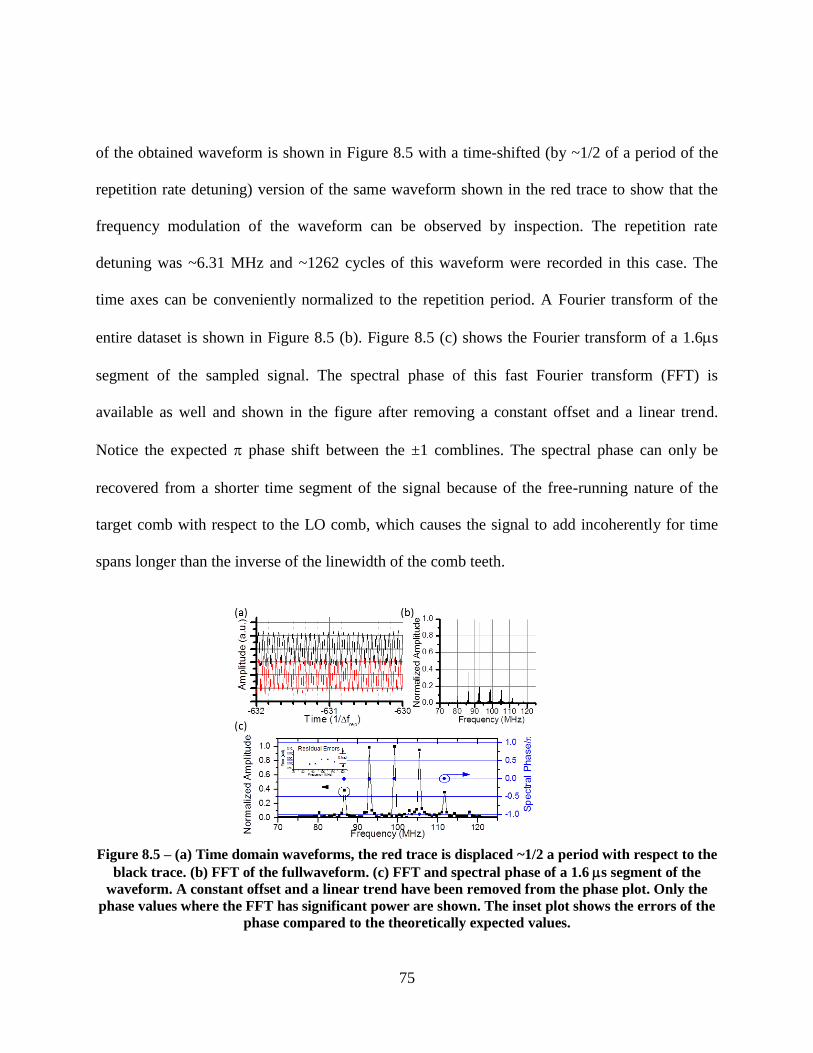
75
of the obtained waveform is shown in Figure 8.5 with a time-shifted (by ~1/2 of a period of the
repetition rate detuning) version of the same waveform shown in the red trace to show that the
frequency modulation of the waveform can be observed by inspection. The repetition rate
detuning was ~6.31 MHz and ~1262 cycles of this waveform were recorded in this case. The
time axes can be conveniently normalized to the repetition period. A Fourier transform of the
entire dataset is shown in Figure 8.5 (b). Figure 8.5 (c) shows the Fourier transform of a 1.6s
segment of the sampled signal. The spectral phase of this fast Fourier transform (FFT) is
available as well and shown in the figure after removing a constant offset and a linear trend.
Notice the expected phase shift between the ±1 comblines. The spectral phase can only be
recovered from a shorter time segment of the signal because of the free-running nature of the
target comb with respect to the LO comb, which causes the signal to add incoherently for time
spans longer than the inverse of the linewidth of the comb teeth.
Figure 8.5 – (a) Time domain waveforms, the red trace is displaced ~1/2 a period with respect to the
black trace. (b) FFT of the fullwaveform. (c) FFT and spectral phase of a 1.6 s segment of the
waveform. A constant offset and a linear trend have been removed from the phase plot. Only the
phase values where the FFT has significant power are shown. The inset plot shows the errors of the
phase compared to the theoretically expected values.
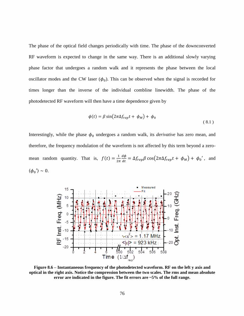
76
The phase of the optical field changes periodically with time. The phase of the downconverted
RF waveform is expected to change in the same way. There is an additional slowly varying
phase factor that undergoes a random walk and it represents the phase between the local
oscillator modes and the CW laser ( ). This can be observed when the signal is recorded for
times longer than the inverse of the individual combline linewidth. The phase of the
photodetected RF waveform will then have a time dependence given by
( ) ( )
( 8.1 )
Interestingly, while the phase undergoes a random walk, its derivative has zero mean, and
therefore, the frequency modulation of the waveform is not affected by this term beyond a zero-
mean random quantity. That is, ( )
( ) , and
⟨ ⟩ .
Figure 8.6 – Instantaneous frequency of the photodetected waveform. RF on the left y axis and
optical in the right axis. Notice the compression between the two scales. The rms and mean absolute
error are indicated in the figure. The fit errors are ~5% of the full range.
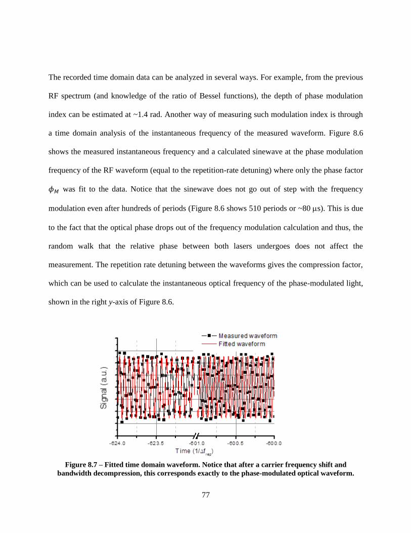
77
The recorded time domain data can be analyzed in several ways. For example, from the previous
RF spectrum (and knowledge of the ratio of Bessel functions), the depth of phase modulation
index can be estimated at ~1.4 rad. Another way of measuring such modulation index is through
a time domain analysis of the instantaneous frequency of the measured waveform. Figure 8.6
shows the measured instantaneous frequency and a calculated sinewave at the phase modulation
frequency of the RF waveform (equal to the repetition-rate detuning) where only the phase factor
was fit to the data. Notice that the sinewave does not go out of step with the frequency
modulation even after hundreds of periods (Figure 8.6 shows 510 periods or ~80 s). This is due
to the fact that the optical phase drops out of the frequency modulation calculation and thus, the
random walk that the relative phase between both lasers undergoes does not affect the
measurement. The repetition rate detuning between the waveforms gives the compression factor,
which can be used to calculate the instantaneous optical frequency of the phase-modulated light,
shown in the right y-axis of Figure 8.6.
Figure 8.7 – Fitted time domain waveform. Notice that after a carrier frequency shift and
bandwidth decompression, this corresponds exactly to the phase-modulated optical waveform.
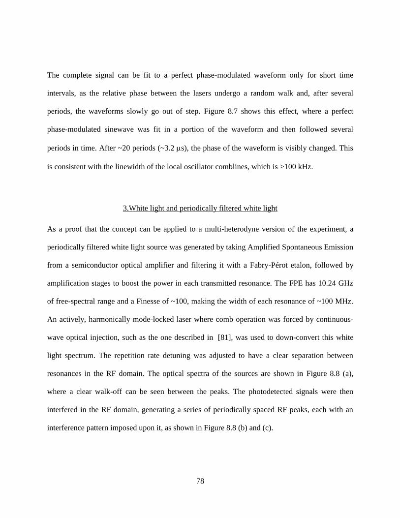
78
The complete signal can be fit to a perfect phase-modulated waveform only for short time
intervals, as the relative phase between the lasers undergo a random walk and, after several
periods, the waveforms slowly go out of step. Figure 8.7 shows this effect, where a perfect
phase-modulated sinewave was fit in a portion of the waveform and then followed several
periods in time. After ~20 periods (~3.2 s), the phase of the waveform is visibly changed. This
is consistent with the linewidth of the local oscillator comblines, which is >100 kHz.
3.White light and periodically filtered white light
As a proof that the concept can be applied to a multi-heterodyne version of the experiment, a
periodically filtered white light source was generated by taking Amplified Spontaneous Emission
from a semiconductor optical amplifier and filtering it with a Fabry-Pérot etalon, followed by
amplification stages to boost the power in each transmitted resonance. The FPE has 10.24 GHz
of free-spectral range and a Finesse of ~100, making the width of each resonance of ~100 MHz.
An actively, harmonically mode-locked laser where comb operation was forced by continuous-
wave optical injection, such as the one described in [81], was used to down-convert this white
light spectrum. The repetition rate detuning was adjusted to have a clear separation between
resonances in the RF domain. The optical spectra of the sources are shown in Figure 8.8 (a),
where a clear walk-off can be seen between the peaks. The photodetected signals were then
interfered in the RF domain, generating a series of periodically spaced RF peaks, each with an
interference pattern imposed upon it, as shown in Figure 8.8 (b) and (c).

79
Figure 8.8 – Multiheterodyne white light interferometry. (a) Optical spectra of the periodically
filtered white light (blue) and the mode-locked laser (red). (b) RF spectra of the interfering
photocurrents of the downconverted white light.
An experiment was performed where the photocurrents were sampled independently and then
interfered. The results are shown in Figure 8.9. A delay of ~12 m of fiber was added between the
two arms and the waveforms sampled in two independent channels of a high-bandwidth
oscilloscope. The sampled waveforms are shown in Figure 8.9 (b). It is interesting to note that
while each of the waveforms is essentially noise (incoherent), the two waveforms are correlated
with a delay of ~63 ns. The FFT spectra of these signals are shown in Figure 8.9 (c). When the
signals are added, spectral interference can be observed in each of the down-converted ASE
peaks. Figure 8.9 (d) shows the resulting interference. The transfer function of a spectral
interferometer is shown in red for visual aid.
Since the interference pattern is sensitive to small path length deviations, another test was made
where a single ASE peak and a continuous wave laser were used to measure the spectrogram of
the interference while the optical path in one of the arms of the interferometer was driven by a
piezo-electric fiber stretcher, as shown in Figure 8.10 (a). The spectrogram in Figure 8.10 (b) is
obtained by calculating the interference pattern while a slow triangular modulation is imposed on

80
ΔtA. The function driving ΔtA is a 1 Hz triangular wave with a peak-to-peak amplitude of 4 fs.
That is, the path delay between the two ASE paths is only changed by 4 fs (ΔtA = 20ns ± 2fs) or,
close to a single cycle of a 200 THz carrier. The experimentally obtained spectrogram is shown
in Figure 8.10 (c), where a clear periodic shift in the fringes is observed with a frequency of 1Hz.
Figure 8.9 – Spectral interference of downconverted incoherent light. (a) Experimental setup. (b)
Sampled RF waveforms. (c) Power spectra of the sampled waveforms. (d) Spectral interference
with superposed transfer function of a spectral interferometer (red).
In conclusion, we have shown a series of experiments where the use of a comb source as a local
oscillator to down-convert and compress optical signals is desirable. We have provided examples
with coherent (too narrow-band to be observed in short observation times) sources where we
have compressed the spectrum of phase modulated light waveforms by factors of ~1600x and
mode-locked pulses by ~17,000x. The carrier frequencies were down-converted from the ~200
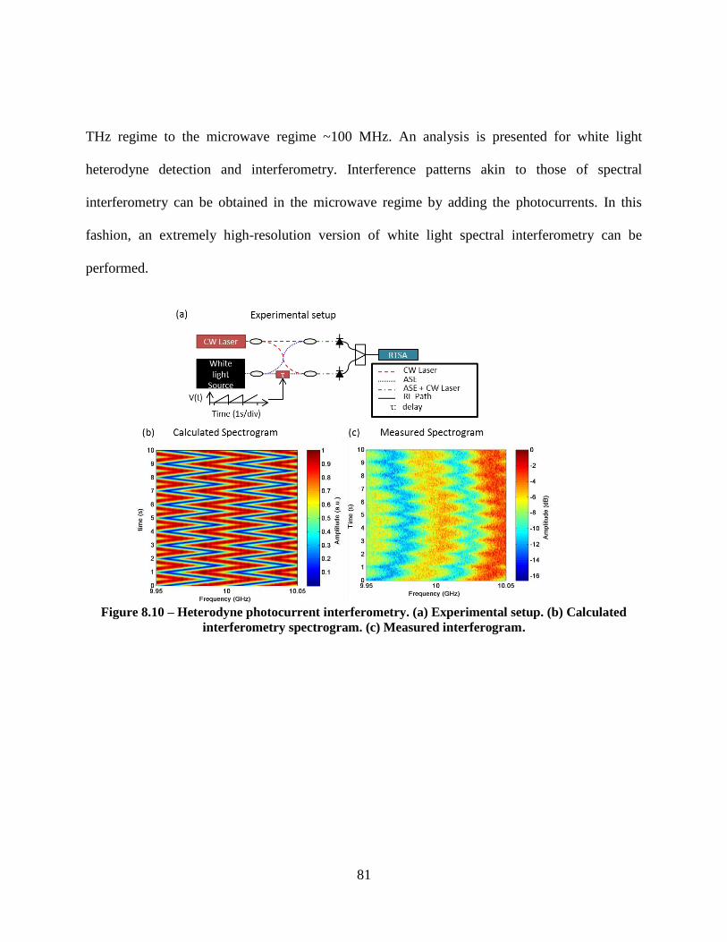
81
THz regime to the microwave regime ~100 MHz. An analysis is presented for white light
heterodyne detection and interferometry. Interference patterns akin to those of spectral
interferometry can be obtained in the microwave regime by adding the photocurrents. In this
fashion, an extremely high-resolution version of white light spectral interferometry can be
performed.
Figure 8.10 – Heterodyne photocurrent interferometry. (a) Experimental setup. (b) Calculated
interferometry spectrogram. (c) Measured interferogram.
82
REFERENCES
1. J. Ye and S. T. Cundiff, Femtosecond Optical Frequency Comb: Principle, Operation,
and Applications (Springer Verlag, 2005).
2. D. J. Jones, S. A. Diddams, J. K. Ranka, A. Stentz, R. S. Windeler, J. L. Hall, and S. T.
Cundiff, "Carrier-Envelope Phase Control of Femtosecond Mode-Locked Lasers and
Direct Optical Frequency Synthesis," Science 288, 635–639 (2000).
3. R. Holzwarth, T. Udem, T. Hänsch, J. Knight, W. Wadsworth, and P. Russell, "Optical
Frequency Synthesizer for Precision Spectroscopy," Physical Review Letters 85, 2264–
2267 (2000).
4. S. Diddams, D. Jones, J. Ye, S. Cundiff, J. Hall, J. Ranka, R. Windeler, R. Holzwarth, T.
Udem, and T. Hansch, "Direct link between microwave and optical frequencies with a 300
THz femtosecond laser comb," Physical review letters 84, 5102–5 (2000).
5. T. Rosenband, D. B. Hume, P. O. Schmidt, C. W. Chou, A. Brusch, L. Lorini, W. H.
Oskay, R. E. Drullinger, T. M. Fortier, J. E. Stalnaker, S. A. Diddams, W. C. Swann, N.
R. Newbury, W. M. Itano, D. J. Wineland, and J. C. Bergquist, "Frequency ratio of Al+
and Hg+ single-ion optical clocks; metrology at the 17th decimal place.," Science (New
York, N.Y.) 319, 1808–12 (2008).
6. C. Parthey, A. Matveev, J. Alnis, B. Bernhardt, A. Beyer, R. Holzwarth, A. Maistrou, R.
Pohl, K. Predehl, T. Udem, T. Wilken, N. Kolachevsky, M. Abgrall, D. Rovera, C.
Salomon, P. Laurent, and T. Hänsch, "Improved Measurement of the Hydrogen 1S–2S
Transition Frequency," Physical Review Letters 107, 1–5 (2011).
7. P. Gill, "Optical clocks coming of age," Nature 407, 579–80 (2000).
8. T. Udem, S. Diddams, K. Vogel, C. Oates, E. Curtis, W. Lee, W. Itano, R. Drullinger, J.
Bergquist, and L. Hollberg, "Absolute Frequency Measurements of the Hg+ and Ca
Optical Clock Transitions with a Femtosecond Laser," Physical Review Letters 86, 4996–
4999 (2001).
9. T. W. Neely, T. A. Johnson, and S. A. Diddams, "High-power broadband laser source
tunable from 30 μm to 44 μmbased on a femtosecond Yb:fiber oscillator," Optics Letters
36, 4020 (2011).
10. F. Adler, P. Masłowski, A. Foltynowicz, K. C. Cossel, T. C. Briles, I. Hartl, and J. Ye,
"Mid-infrared Fourier transform spectroscopy with a broadband frequency comb," Optics
Express 18, 21861 (2010).

83
11. A. Schliesser, M. Brehm, F. Keilmann, and D. W. van der Weide, "Frequency-comb
infrared spectrometer for rapid, remote chemical sensing," Optics Express 13, 9029
(2005).
12. A. Schliesser, N. Picqué, and T. W. Hänsch, "Mid-infrared frequency combs," Nature
Photonics 6, 440–449 (2012).
13. C. Gohle, T. Udem, M. Herrmann, J. Rauschenberger, R. Holzwarth, H. a Schuessler, F.
Krausz, and T. W. Hänsch, "A frequency comb in the extreme ultraviolet.," Nature 436,
234–7 (2005).
14. D. Z. Kandula, C. Gohle, T. J. Pinkert, W. Ubachs, and K. S. E. Eikema, "XUV frequency
comb metrology on the ground state of helium," 18 (2011).
15. T. K. Allison, A. Cingöz, D. C. Yost, and J. Ye, "Extreme Nonlinear Optics in a
Femtosecond Enhancement Cavity," America 1–10 (2011).
16. M. Fischer, N. Kolachevsky, M. Zimmermann, R. Holzwarth, T. Udem, T. W. Hänsch, M.
Haas, U. D. Jentschura, and C. H. Keitel, "New Limits on the Drift of Fundamental
Constants from Laboratory Measurements," Physical Review Letters 92, 1–4 (2004).
17. T. Steinmetz, T. Wilken, C. Araujo-Hauck, R. Holzwarth, T. W. Hänsch, L. Pasquini, A.
Manescau, S. D’Odorico, M. T. Murphy, T. Kentischer, W. Schmidt, and T. Udem, "Laser
frequency combs for astronomical observations.," Science (New York, N.Y.) 321, 1335–7
(2008).
18. D. A. Braje, M. S. Kirchner, S. Osterman, T. Fortier, and S. A. Diddams, "Astronomical
spectrograph calibration with broad-spectrum frequency combs," The European Physical
Journal D 48, 57–66 (2008).
19. G. Walker, "Extrasolar planets: with a coarse-tooth comb.," Nature 452, 538–9 (2008).
20. I. Coddington, W. C. Swann, L. Nenadovic, and N. R. Newbury, "Rapid and precise
absolute distance measurements at long range," Nature Photonics 3, 351–356 (2009).
21. S.-W. Kim, "Metrology: Combs rule," Nature Photonics 3, 313–314 (2009).
22. S. Schiller, "Spectrometry with frequency combs," Optics letters 27, 766–8 (2002).
23. I. Coddington, W. Swann, and N. Newbury, "Coherent Multiheterodyne Spectroscopy
Using Stabilized Optical Frequency Combs," Physical Review Letters 100, (2008).
24. N. R. Newbury, I. Coddington, and W. Swann, "Sensitivity of coherent dual-comb
spectroscopy.," Optics express 18, 7929–45 (2010).

84
25. B. Bernhardt, A. Ozawa, P. Jacquet, M. Jacquey, Y. Kobayashi, N. Picque, T. Udem, R.
Holzwarth, G. Guelachvili, and T. W. Ha, "Cavity-enhanced dual-comb spectroscopy," 4,
2009–2011 (2010).
26. T. Ideguchi, A. Poisson, G. Guelachvili, N. Picqué, and W. Theodor, "Adaptive real-time
dual-comb spectroscopy," Sciences-New York 1–6 (n.d.).
27. P. J. Delfyett, S. Gee, H. Izadpanah, S. Ozharar, F. Quinlan, and T. Yilmaz, "Optical
frequency combs from semiconductor lasers and applications in ultrawideband signal
processing and communications," Journal of Lightwave Technology 24, 2701–2719
(2006).
28. P. J. Delfyett, I. Ozdur, N. Hoghooghi, M. Akbulut, J. Davila-Rodriguez, and S.
Bhooplapur, "Advanced Ultrafast Technologies Based on Optical Frequency Combs,"
IEEE Journal of Selected Topics in Quantum Electronics 1–17 (2011).
29. A. M. Weiner, "Femtosecond pulse shaping using spatial light modulators," Review of
Scientific Instruments 71, 1929 (2000).
30. G. C. Valley, "Photonic analog-to-digital converters.," Optics express 15, 1955–82 (2007).
31. H. Taylor, "An optical analog-to-digital converter--Design and analysis," IEEE Journal of
Quantum Electronics 15, 210–216 (1979).
32. T. M. Fortier, M. S. Kirchner, F. Quinlan, J. Taylor, J. C. Bergquist, T. Rosenband, N.
Lemke, a. Ludlow, Y. Jiang, C. W. Oates, and S. a. Diddams, "Generation of ultrastable
microwaves via optical frequency division," Nature Photonics 5, 425–429 (2011).
33. J. Millo, R. Boudot, M. Lours, P. Y. Bourgeois, A. N. Luiten, Y. Le Coq, Y. Kersalé, and
G. Santarelli, "Ultra-low-noise microwave extraction from fiber-based optical frequency
comb.," Optics letters 34, 3707–9 (2009).
34. A. Haboucha, W. Zhang, T. Li, M. Lours, A. N. Luiten, Y. Le Coq, and G. Santarelli,
"Optical-fiber pulse rate multiplier for ultralow phase-noise signal generation.," Optics
letters 36, 3654–6 (2011).
35. F. Quinlan, S. Ozharar, S. Gee, and P. J. Delfyett, "Harmonically mode-locked
semiconductor-based lasers as high repetition rate ultralow noise pulse train and optical
frequency comb sources," Journal of Optics A: Pure and Applied Optics 11, 103001
(2009).
36. T. Yilmaz, C. M. Depriest, a. Braun, J. H. Abeles, and P. J. Delfyett, "Noise in
fundamental and harmonic modelocked semiconductor lasers: Experiments and
simulations," IEEE Journal of Quantum Electronics 39, 838–849 (2003).
85
37. T. Yilmaz, C. Depriest, P. Delfyett, S. Etemad, a Braun, and J. Abeles, "Supermode
suppression to below -130 dBc/Hz in a 10 GHz harmonically mode-locked external sigma
cavity semiconductor laser.," Optics express 11, 1090–5 (2003).
38. S. Gee, F. Quinlan, S. Ozharar, and P. J. Delfyett, "Correlation of supermode noise of
harmonically mode-locked lasers," Journal of the Optical Society of America B 24, 1490
(2007).
39. F. Rana, H. L. T. Lee, R. J. Ram, M. E. Grein, L. A. Jiang, E. P. Ippen, and H. A. Haus,
"Characterization of the noise and correlations in harmonically mode-locked lasers,"
Journal of the Optical Society of America B 19, 2609 (2002).
40. L. A. Jiang, E. P. Ippen, and H. Yokoyama, "Semiconductor mode-locked lasers as pulse
sources for high bit rate data transmission," Journal of Optical and Fiber Communications
Reports 2, 1–31 (2005).
41. G. Roelkens, L. Liu, D. Liang, R. Jones, a. Fang, B. Koch, and J. Bowers, "III-V/silicon
photonics for on-chip and intra-chip optical interconnects," Laser & Photonics Reviews 4,
751–779 (2010).
42. S. R. Jain, M. N. Sysak, G. Kurczveil, and J. E. Bowers, "Integrated hybrid silicon DFB
laser-EAM array using quantum well intermixing.," Optics express 19, 13692–9 (2011).
43. S. Gee, F. Quinlan, S. Ozharar, and P. J. Delfyett, "Simultaneous optical comb frequency
stabilization and super-mode noise suppression of harmonically mode-locked
semiconductor ring laser using an intracavity etalon," IEEE Photonics Technology Letters
17, 199–201 (2005).
44. E. Rubiola and V. Giordano, "Advanced interferometric phase and amplitude noise
measurements," Review of Scientific Instruments 73, 2445 (2002).
45. E. Rubiola, Phase Noise and Frequency Stability in Oscillators (Cambridge University
Press, 2009).
46. E. Rubiola, V. Giordano, and J. Groslambert, "Very high frequency and microwave
interferometric phase and amplitude noise measurements," Review of Scientific
Instruments 70, 220–225 (1999).
47. E. Rubiola, E. Salik, S. Huang, N. Yu, and L. Maleki, "Photonic-delay technique for
phase-noise measurement of microwave oscillators," Journal of the Optical Society of
America B 22, 987 (2005).
48. K. Volyanskiy, J. Cussey, H. Tavernier, P. Salzenstein, G. Sauvage, L. Larger, and E.
Rubiola, "Applications of the optical fiber to the generation and measurement of low-

86
phase-noise microwave signals," Journal of the Optical Society of America B 25, 2140
(2008).
49. F. Quinlan, S. Gee, S. Ozharar, and P. Delfyett, "The effects of filtering RF source phase
noise by a low noise, high quality factor actively modelocked laser on the laser’s absolute
and relative phase noise," Optics Express 14, 5346 (2006).
50. I. Ozdur, M. Akbulut, N. Hoghooghi, D. Mandridis, S. Ozharar, F. Quinlan, and P. J.
Delfyett, "A Semiconductor-Based 10-GHz Optical Comb Source With Sub 3-fs Shot-
Noise-Limited Timing Jitter and ~500-Hz Comb Linewidth," IEEE Photonics Technology
Letters 22, 431–433 (2010).
51. E. D. Black, "An introduction to Pound–Drever–Hall laser frequency stabilization,"
American Journal of Physics 69, 79 (2001).
52. R. W. P. Drever, J. L. Hall, F. V. Kowalski, J. Hough, G. M. Ford, A. J. Munley, and H.
Ward, "Laser phase and frequency stabilization using an optical resonator," Applied
Physics B Photophysics and Laser Chemistry 31, 97–105 (1983).
53. K. Sarwar Abedin, N. Onodera, and M. Hyodo, "Repetition-rate multiplication in actively
mode-locked fiber lasers by higher-order FM mode locking using a high-finesse Fabry–
Perot filter," Applied Physics Letters 73, 1311 (1998).
54. K. S. Abedin, N. Onodera, and M. Hyodo, "Higher order FM mode locking for pulse-
repetition-rate enhancement in actively mode-locked lasers: theory and experiment," IEEE
Journal of Quantum Electronics 35, 875–890 (1999).
55. E. Rubiola, M. Olivier, and J. Groslambert, "Phase noise in the regenerative frequency
dividers," IEEE Transactions on Instrumentation and Measurement 41, 353–360 (1992).
56. N. K. Fontaine, D. J. Geisler, R. P. Scott, T. He, J. P. Heritage, and S. J. B. Yoo,
"Demonstration of high-fidelity dynamic optical arbitrary waveform generation.," Optics
express 18, 22988–95 (2010).
57. R. P. Scott, N. K. Fontaine, J. P. Heritage, and S. J. B. Yoo, "Dynamic optical arbitrary
waveform generation and measurement.," Optics express 18, 18655–70 (2010).
58. R. H. Walden, "Analog-to-digital converter survey and analysis," IEEE Journal on
Selected Areas in Communications 17, 539–550 (1999).
59. P. W. Juodawlkis, J. C. Twichell, G. E. Betts, J. J. Hargreaves, R. D. Younger, J. L.
Wasserman, F. J. O’Donnell, K. G. Ray, and R. C. Williamson, "Optically sampled
analog-to-digital converters," IEEE Transactions on Microwave Theory and Techniques
49, 1840–1853 (2001).
87
60. T. M. Fortier, M. S. Kirchner, F. Quinlan, J. Taylor, J. C. Bergquist, T. Rosenband, N.
Lemke, A. Ludlow, Y. Jiang, C. W. Oates, and S. A. Diddams, "Photonic Generation of
Low-Phase-Noise Microwave Signals," Arxiv:1101.3616 1–17 (2011).
61. F. Quinlan, T. M. Fortier, M. S. Kirchner, J. A. Taylor, M. J. Thorpe, N. Lemke, A. D.
Ludlow, Y. Jiang, and S. A. Diddams, "Ultralow phase noise microwave generation with
an Er:fiber-based optical frequency divider," Optics Letters 36, 3260 (2011).
62. J. Davila-Rodriguez, I. Ozdur, C. Williams, and P. J. Delfyett, "A semiconductor-based,
frequency-stabilized mode-locked laser using a phase modulator and an intracavity
etalon," Optics Letters 35, 4130 (2010).
63. P. W. Juodawlkis, J. J. Plant, W. Loh, L. J. Missaggia, K. E. Jensen, and F. J. O’Donnell,
"Packaged 1.5-µm Quantum-Well SOA With 0.8-W Output Power and 5.5-dB Noise
Figure," IEEE Photonics Technology Letters 21, 1208–1210 (2009).
64. W. Loh, J. J. Plant, J. Klamkin, J. P. Donnelly, F. J. O’Donnell, R. J. Ram, and P. W.
Juodawlkis, "Noise Figure of Watt-Class Ultralow-Confinement Semiconductor Optical
Amplifiers," IEEE Journal of Quantum Electronics 47, 66–75 (2011).
65. S. Gee, F. Quinlan, S. Ozharar, P. J. Delfyett, J. J. Plant, and P. W. Juodawlkis, "Ultralow-
noise mode-locked optical pulse trains from an external cavity laser based on a slab
coupled optical waveguide amplifier (SCOWA)," Optics Letters 30, 2742 (2005).
66. Z. Jiang, D. S. Seo, D. E. Leaird, and a M. Weiner, "Spectral line-by-line pulse shaping.,"
Optics letters 30, 1557–9 (2005).
67. a. M. Zolot, F. R. Giorgetta, E. Baumann, J. W. Nicholson, W. C. Swann, I. Coddington,
and N. R. Newbury, "Direct-comb molecular spectroscopy with accurate, resolved comb
teeth over 43 THz," Optics Letters 37, 638 (2012).
68. F. Quinlan, S. Gee, S. Ozharar, and P. J. Delfyett, "Ultralow-jitter and -amplitude-noise
semiconductor-based actively mode-locked laser," Optics Letters 31, 2870 (2006).
69. S. A. Diddams, L.-S. Ma, J. Ye, and J. L. Hall, "Broadband optical frequency comb
generation with a phase-modulated parametric oscillator," Optics Letters 24, 1747 (1999).
70. T. Udem, J. Reichert, R. Holzwarth, and T. W. Hänsch, "Accurate measurement of large
optical frequency differences with a mode-locked laser," Optics Letters 24, 881 (1999).
71. T. Udem, R. Holzwarth, and T. W. Hänsch, "Optical frequency metrology.," Nature 416,
233–7 (2002).

88
72. M. Akbulut, S. Bhooplapur, I. Ozdur, J. Davila-Rodriguez, and P. J. Delfyett, "Dynamic
line-by-line pulse shaping with GHz update rate.," Optics express 18, 18284–91 (2010).
73. S. Bhooplapur, N. Hoghooghi, and P. J. Delfyett, "Pulse shapes reconfigured on a pulse-
to-pulse time scale by using an array of injection-locked VCSELs.," Optics letters 36,
1887–9 (2011).
74. I. Coddington, W. C. Swann, and N. R. Newbury, "Coherent linear optical sampling at 15
bits of resolution.," Optics letters 34, 2153–5 (2009).
75. F. Ferdous, D. E. Leaird, C.-B. Huang, and A. M. Weiner, "Dual-comb electric-field
cross-correlation technique for optical arbitrary waveform characterization.," Optics
letters 34, 3875–7 (2009).
76. F. R. Giorgetta, I. Coddington, E. Baumann, W. C. Swann, and N. R. Newbury, "Fast
high-resolution spectroscopy of dynamic continuous-wave laser sources," Nature
Photonics 4, 853–857 (2010).
77. A. D. Ludlow, X. Huang, M. Notcutt, T. Zanon-Willette, S. M. Foreman, M. M. Boyd, S.
Blatt, and J. Ye, "Compact, thermal-noise-limited optical cavity for diode laser
stabilization at 1x10(-15).," Optics letters 32, 641–3 (2007).
78. Y. Y. Jiang, A. D. Ludlow, N. D. Lemke, R. W. Fox, J. A. Sherman, L.-S. Ma, and C. W.
Oates, "Making optical atomic clocks more stable with 10−16-level laser stabilization,"
Nature Photonics 3–6 (2011).
79. B. Young, F. Cruz, W. Itano, and J. Bergquist, "Visible Lasers with Subhertz Linewidths,"
Physical Review Letters 82, 3799–3802 (1999).
80. R. Hanbury Brown and R. Q. Twiss, "Interferometry of the Intensity Fluctuations in Light.
I. Basic Theory: The Correlation between Photons in Coherent Beams of Radiation,"
Proceedings of the Royal Society A: Mathematical, Physical and Engineering Sciences
242, 300–324 (1957).
81. C. Williams, F. Quinlan, and P. J. Delfyett, "Injection-Locked Mode-Locked Laser With
Long-Term Stabilization and High Power-per-Combline," IEEE Photonics Technology
Letters 21, 94–96 (2009).