extended sibships danielle posthuma kate morley files: \\danielle\extsibs
Post on 20-Dec-2015
236 views
TRANSCRIPT
Extended sibships
Danielle PosthumaKate Morley
Files: \\danielle\ExtSibs
TC 19 - Boulder 2006
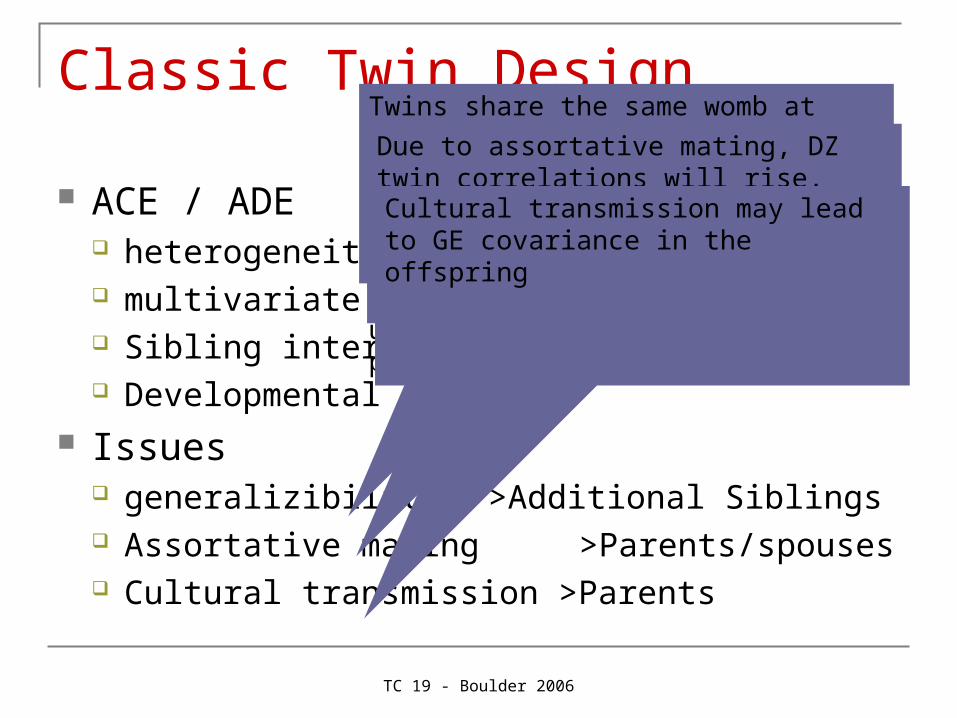
Classic Twin Design
ACE / ADE heterogeneity multivariate Sibling interaction Developmental
Issues generalizibility >Additional Siblings Assortative mating >Parents/spouses Cultural transmission >Parents
Twins share the same womb at the same time, this may not only make them more similar, but sharing the womb itself may also lead to complications specific to twin births, rendering twins unrepresentative of the normal population
Due to assortative mating, DZ twin correlations will rise, leading to increased estimates of C.Cultural transmission may lead to GE covariance in the offspring
TC 19 - Boulder 2006
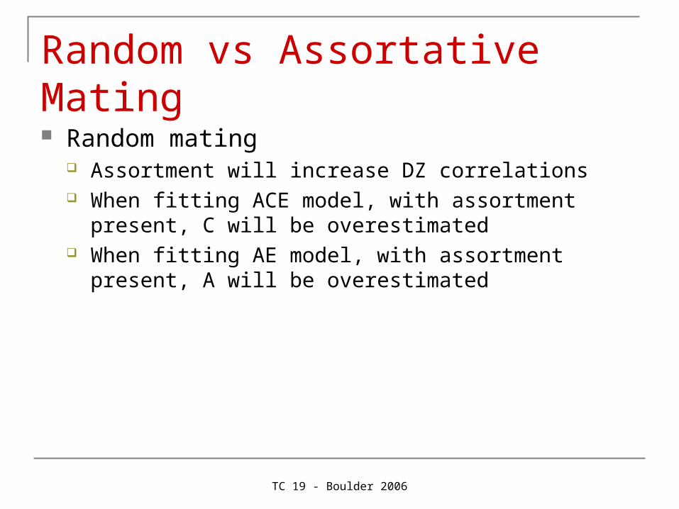
Random vs Assortative Mating Random mating
Assortment will increase DZ correlations When fitting ACE model, with assortment present, C will be
overestimated When fitting AE model, with assortment present, A will be
overestimated
TC 19 - Boulder 2006
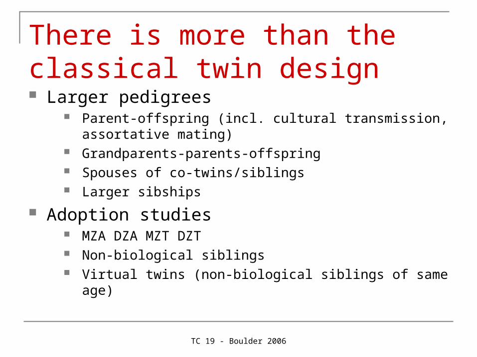
There is more than the classical twin design Larger pedigrees
Parent-offspring (incl. cultural transmission, assortative mating)
Grandparents-parents-offspring Spouses of co-twins/siblings Larger sibships
Adoption studies MZA DZA MZT DZT Non-biological siblings Virtual twins (non-biological siblings of same age)
Parent - Offspring
TC 19 - Boulder 2006
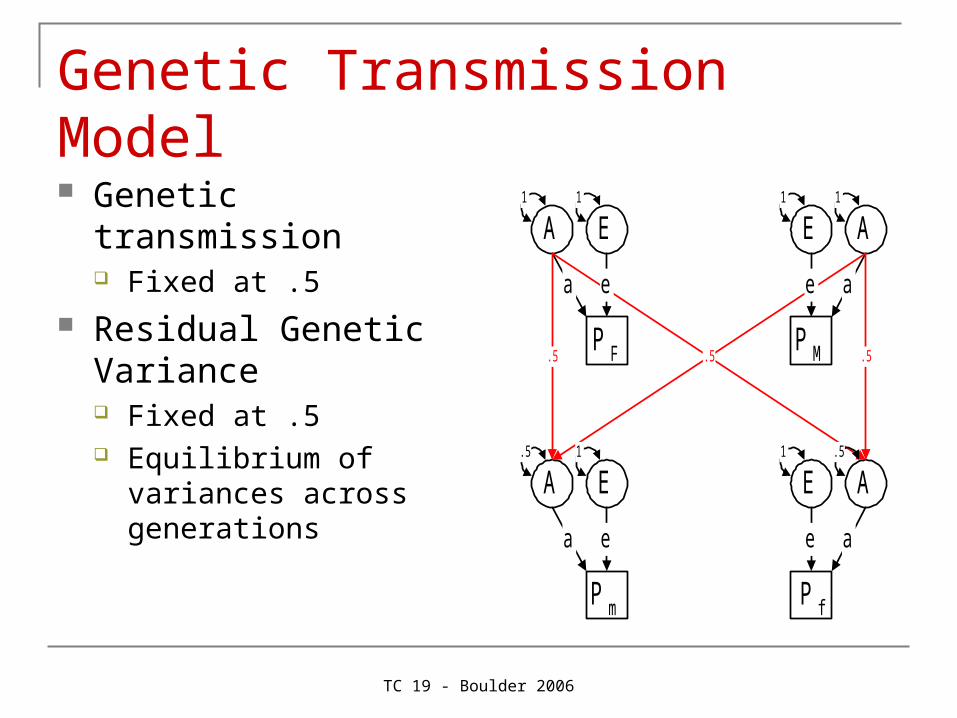
Genetic Transmission Model
Genetic transmission Fixed at .5
Residual Genetic Variance Fixed at .5 Equilibrium of variances
across generations
P M
P m P f
A
A A
A
a a
a a
.5 .5.5.5P F
1
.5
1
.5
E
e
1
E
e
1
E
e
1
E
e
1
TC 19 - Boulder 2006
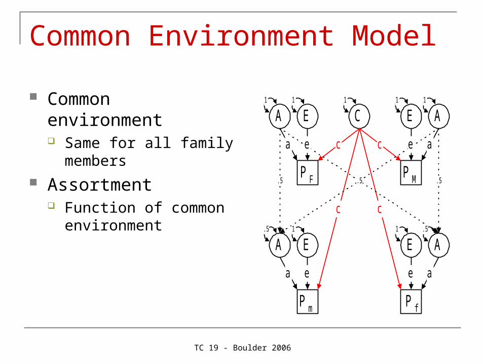
Common Environment Model
Common environment Same for all family
members Assortment
Function of common environment
P M
P m P f
A
A A
A C
a a
a
c c
c c
.5 .5.5.5P F
1
.5
11
.5
E
e
1
E
e
1
E
e
1
E1
ae
TC 19 - Boulder 2006
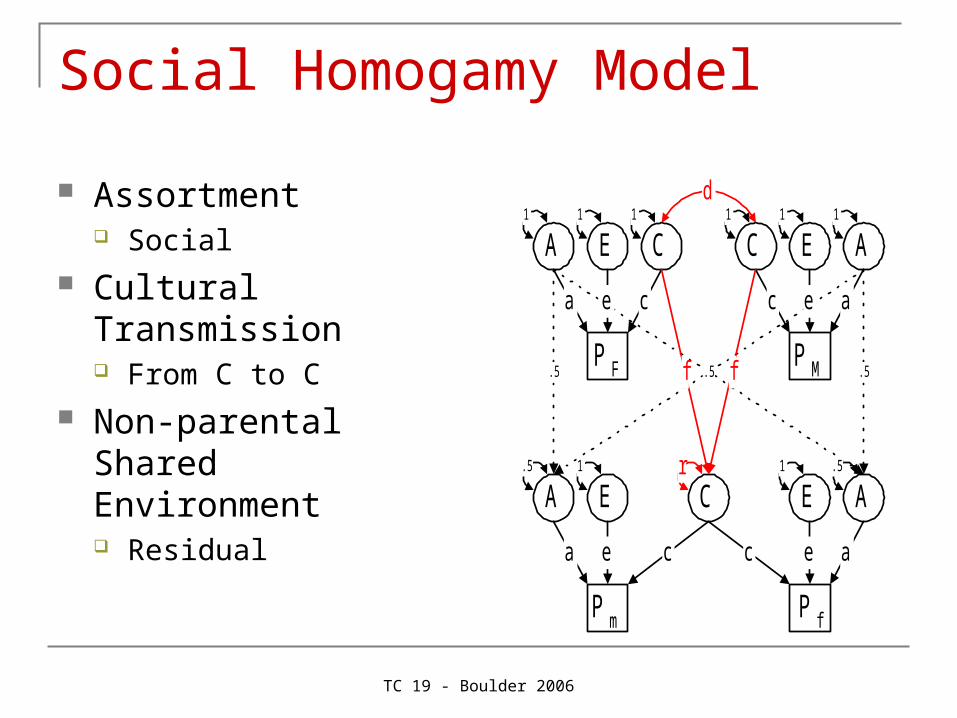
Social Homogamy Model
Assortment Social
Cultural Transmission From C to C
Non-parental Shared Environment Residual
P M
P m P f
A
A A
C
C
A C
a a
a a
c c
c c
.5 .5.5.5P F
1
r .5
111
.5
E
e
1
E
e
1
E
e
1
E
e
1
f f
d
TC 19 - Boulder 2006
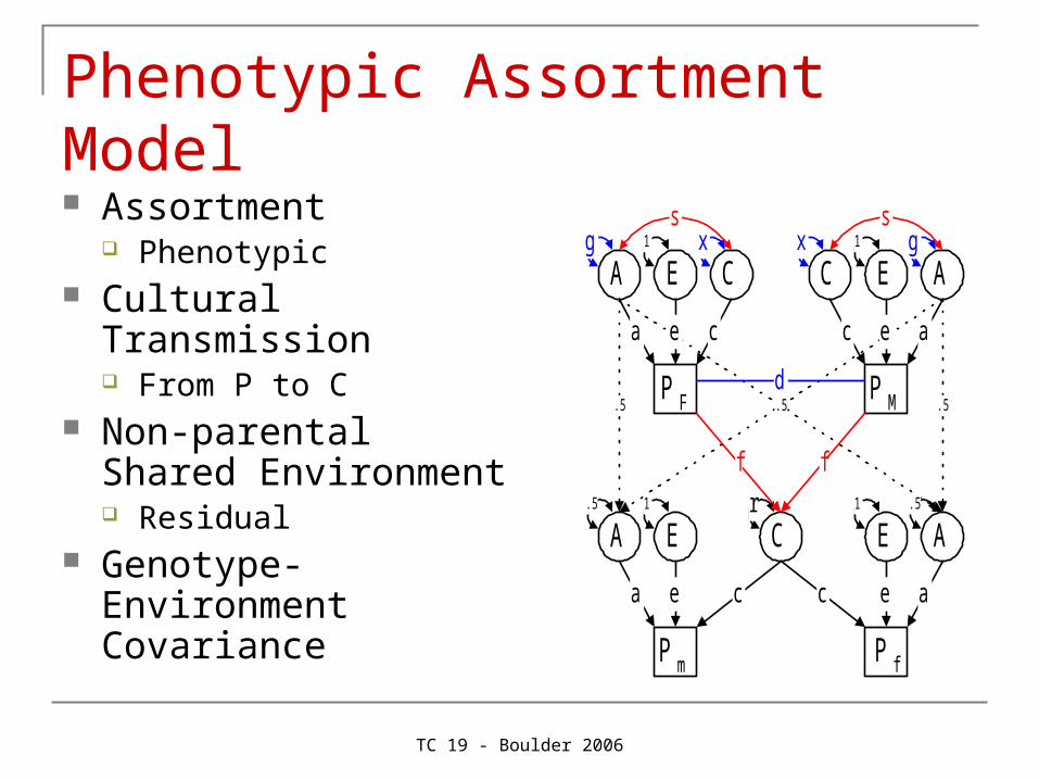
Phenotypic Assortment Model Assortment
Phenotypic Cultural Transmission
From P to C Non-parental Shared
Environment Residual
Genotype-Environment Covariance
P M
P m P f
A
A A
C
C
A C
a a
a a
c c
c c
.5 .5.5.5P F
g
r .5
gxx
.5
E
e
1
E
e
1
E
e
1
E
e
1
f f
d
s s
Spouses and offspring of twins
TC 19 - Boulder 2006
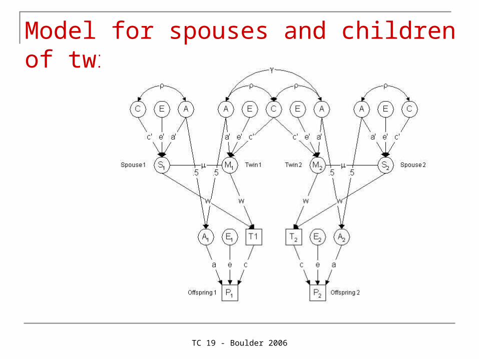
Model for spouses and children of twins (Eaves)
Extended sibships
TC 19 - Boulder 2006
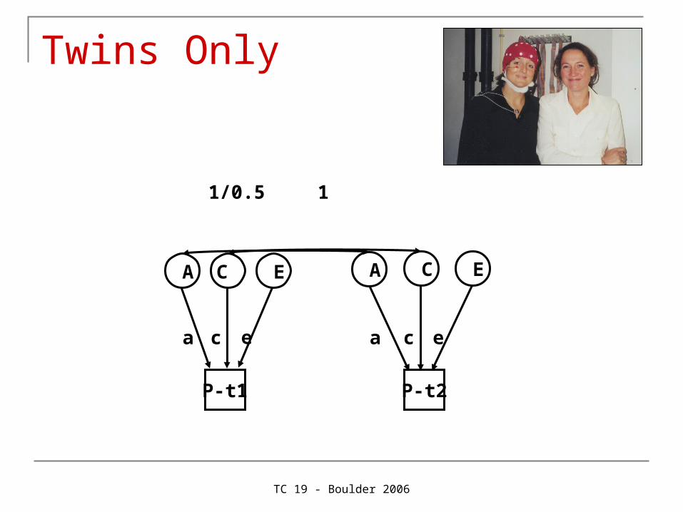
Twins Only
1
P-t1
E AC C A E
ec ecaa
P-t2
1/0.5
TC 19 - Boulder 2006
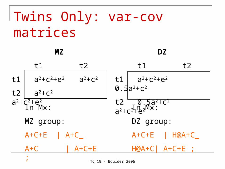
MZ
t1 t2
t1 a2+c2+e2 a2+c2
t2 a2+c2 a2+c2+e2
DZ
t1 t2
t1 a2+c2+e2 0.5a2+c2
t2 0.5a2+c2 a2+c2+e2
In Mx:
MZ group:
A+C+E | A+C_
A+C | A+C+E ;
In Mx:
DZ group:
A+C+E | H@A+C_
H@A+C| A+C+E ;
Twins Only: var-cov matrices
TC 19 - Boulder 2006
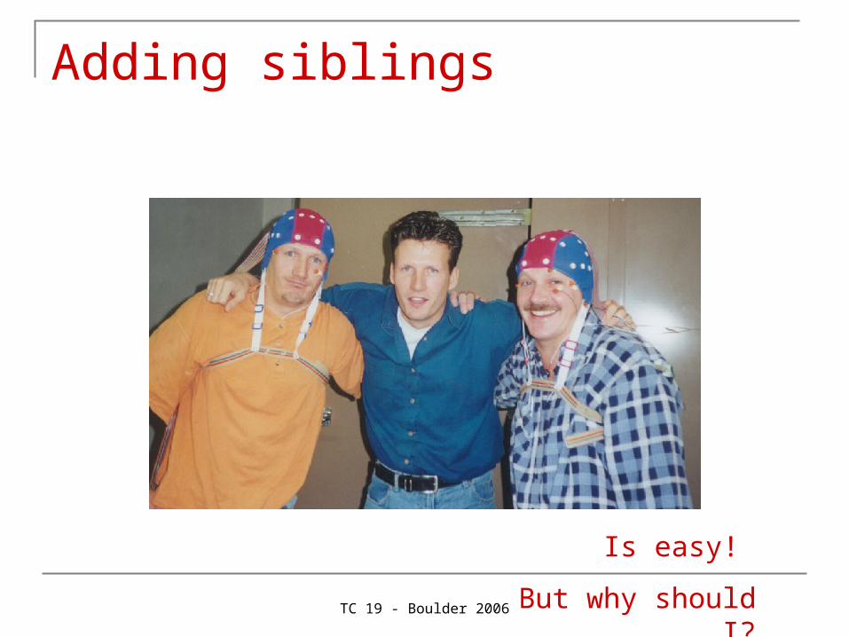
Adding siblings
Is easy!
But why should I?
TC 19 - Boulder 2006
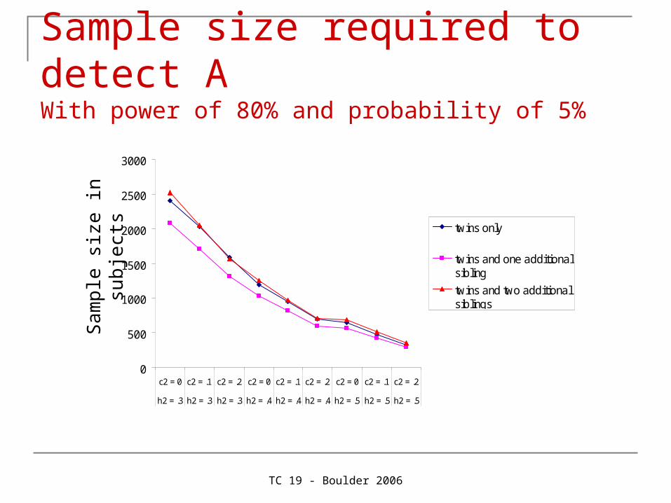
0
500
1000
1500
2000
2500
3000
c2 = 0 c2 = .1 c2 = .2 c2 = 0 c2 = .1 c2 = .2 c2 = 0 c2 = .1 c2 = .2
h2 = .3 h2 = .3 h2 = .3 h2 = .4 h2 = .4 h2 = .4 h2 = .5 h2 = .5 h2 = .5
twins only
twins and one additionalsibling
twins and two additionalsiblings
Sam
ple
size
in s
ubje
cts
Sample size required to detect A With power of 80% and probability of 5%
TC 19 - Boulder 2006
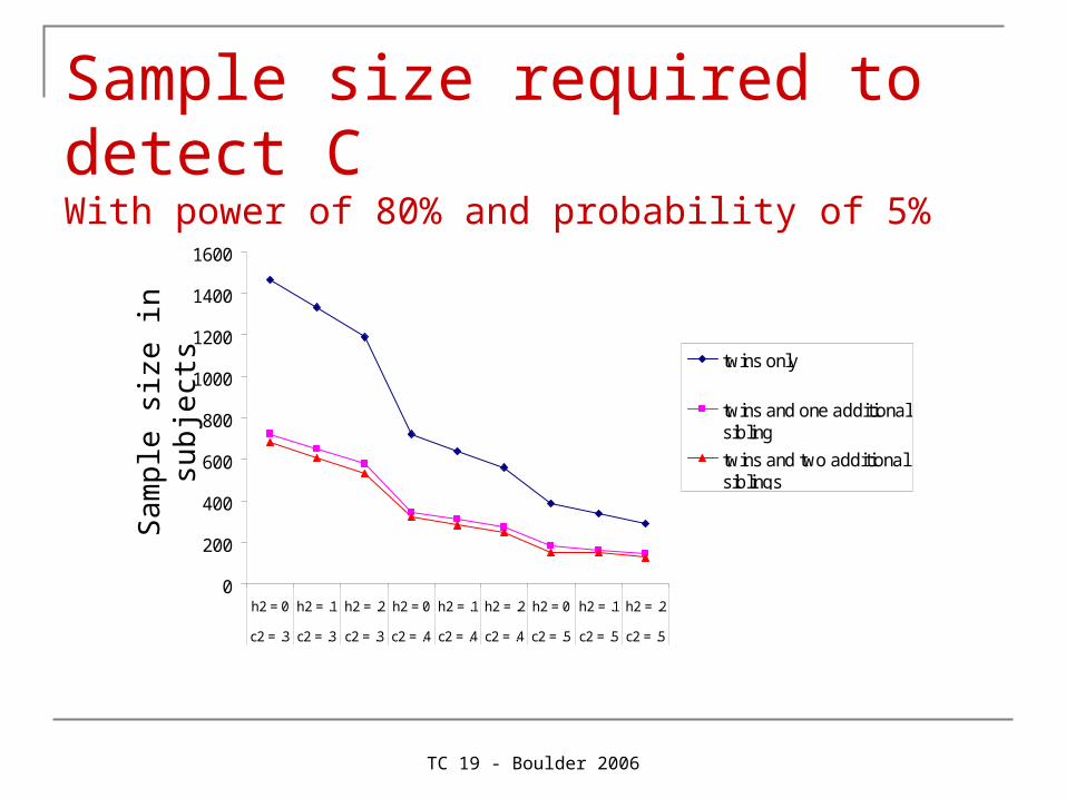
0
200
400
600
800
1000
1200
1400
1600
h2 = 0 h2 = .1 h2 = .2 h2 = 0 h2 = .1 h2 = .2 h2 = 0 h2 = .1 h2 = .2
c2 = .3 c2 = .3 c2 = .3 c2 = .4 c2 = .4 c2 = .4 c2 = .5 c2 = .5 c2 = .5
twins only
twins and one additionalsibling
twins and two additionalsiblings
Sam
ple
size
in s
ubje
cts
Sample size required to detect C With power of 80% and probability of 5%
TC 19 - Boulder 2006
Larger sibships
Provides a bit more power to detect AProvides a lot more power to detect C
Since C is usually small (e.g. A = .60, C = .20, E = .20), C is usually dropped from the model as it is not significant. As C is a familial source of variance, part of it will the end up in A, which will now be overestimated. Therefore, more power for C protects against overestimation of A.
TC 19 - Boulder 2006
Larger sibships
Will also allow you to test certain assumptions such as: Are twins different from singletons with respect to
means? Are twins different from singletons with respect to
variances? Do DZ twins correlate any different than non-twin
sibpairs?
TC 19 - Boulder 2006
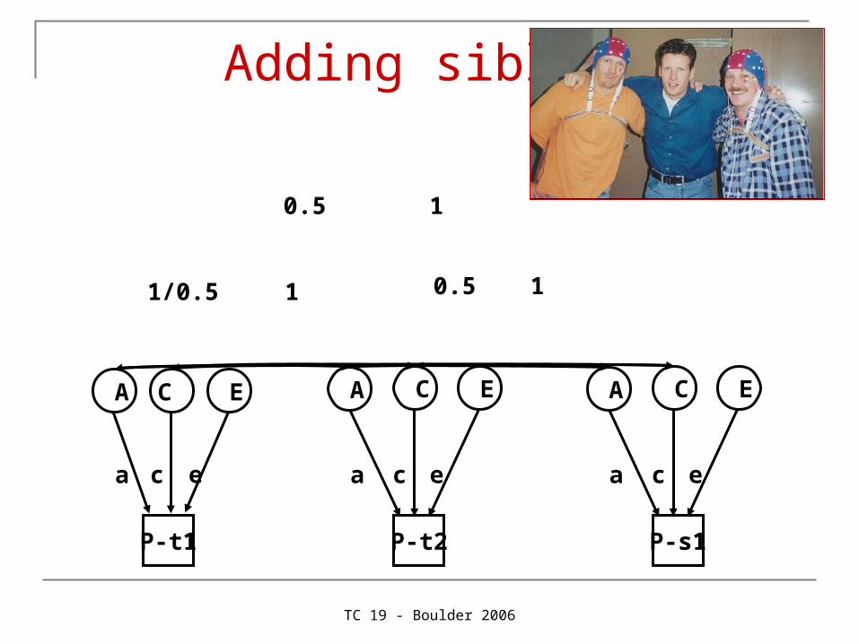
1
P-t1
E AC C A E
ec ecaa
P-t2
1/0.5
A C E
eca
P-s1
10.5
10.5
Adding siblings
TC 19 - Boulder 2006
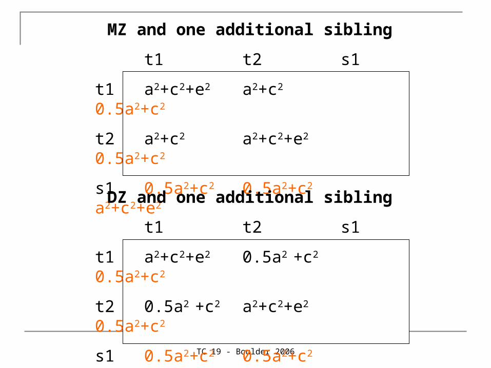
MZ and one additional sibling
t1 t2 s1
t1 a2+c2+e2 a2+c2 0.5a2+c2
t2 a2+c2 a2+c2+e2 0.5a2+c2
s1 0.5a2+c2 0.5a2+c2 a2+c2+e2
DZ and one additional sibling
t1 t2 s1
t1 a2+c2+e2 0.5a2 +c2 0.5a2+c2
t2 0.5a2 +c2 a2+c2+e2 0.5a2+c2
s1 0.5a2+c2 0.5a2+c2 a2+c2+e2
TC 19 - Boulder 2006
.
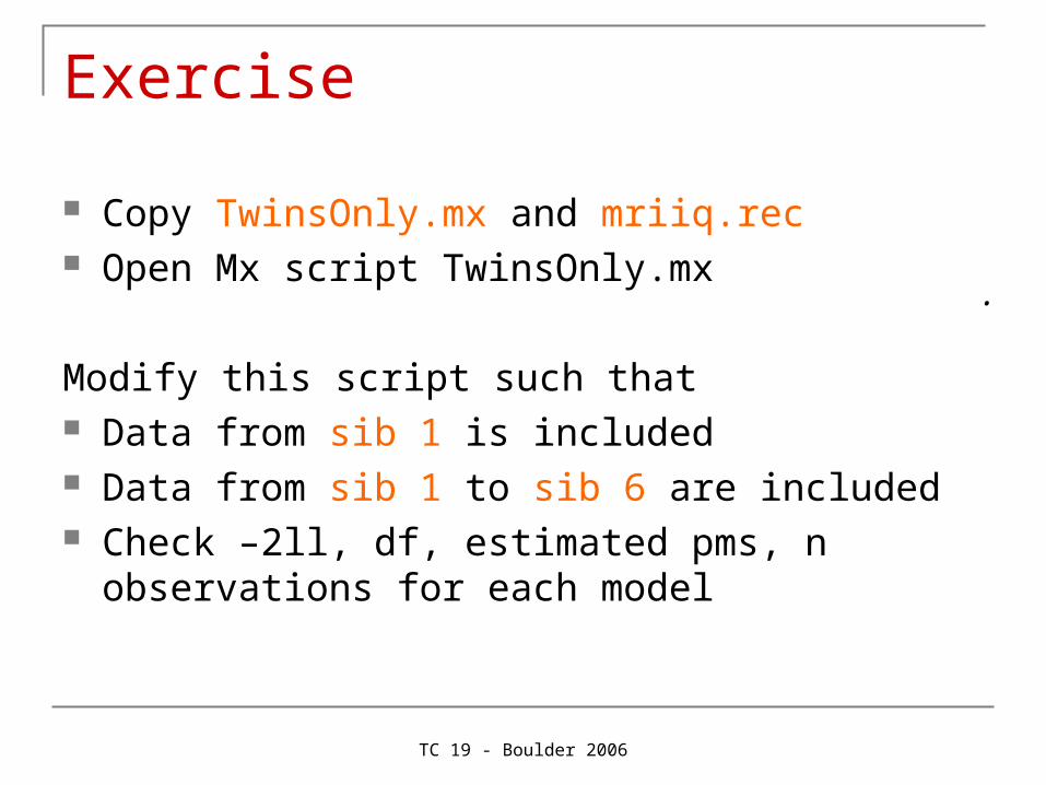
Exercise
Copy TwinsOnly.mx and mriiq.rec Open Mx script TwinsOnly.mx
Modify this script such that Data from sib 1 is included Data from sib 1 to sib 6 are included Check –2ll, df, estimated pms, n observations for
each model
TC 19 - Boulder 2006
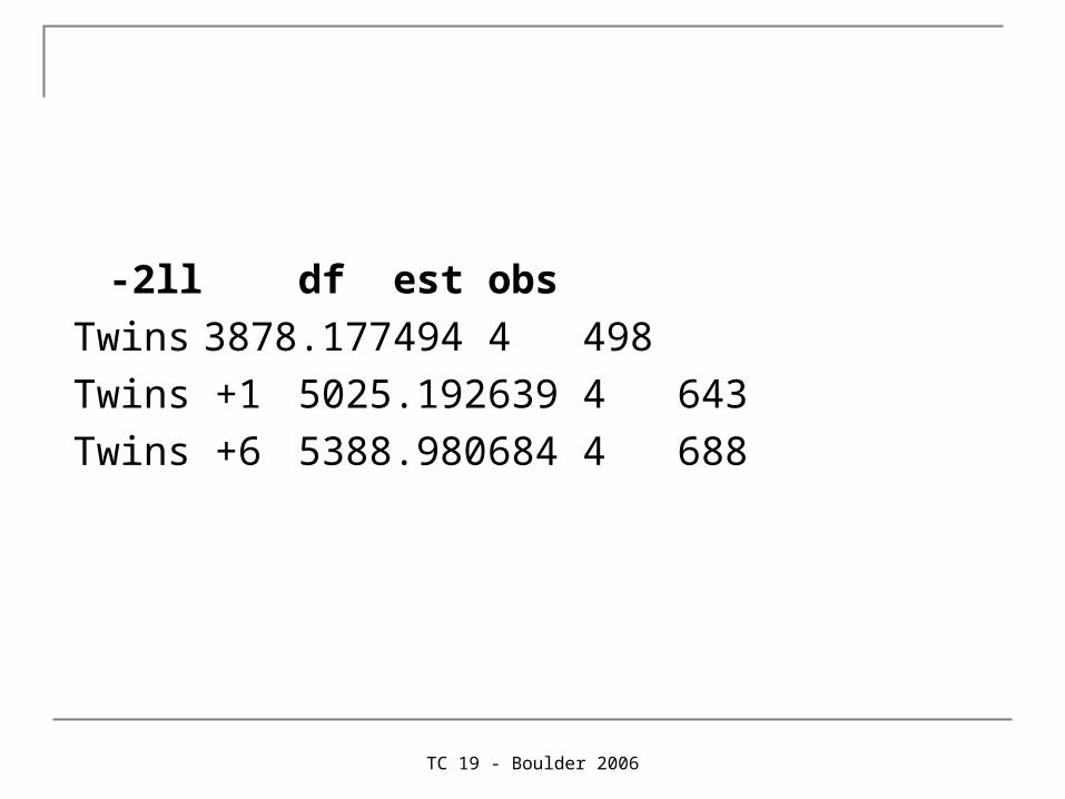
-2ll df est obs
Twins 3878.177 494 4 498
Twins +1 5025.192 639 4 643
Twins +6 5388.980 684 4 688
TC 19 - Boulder 2006
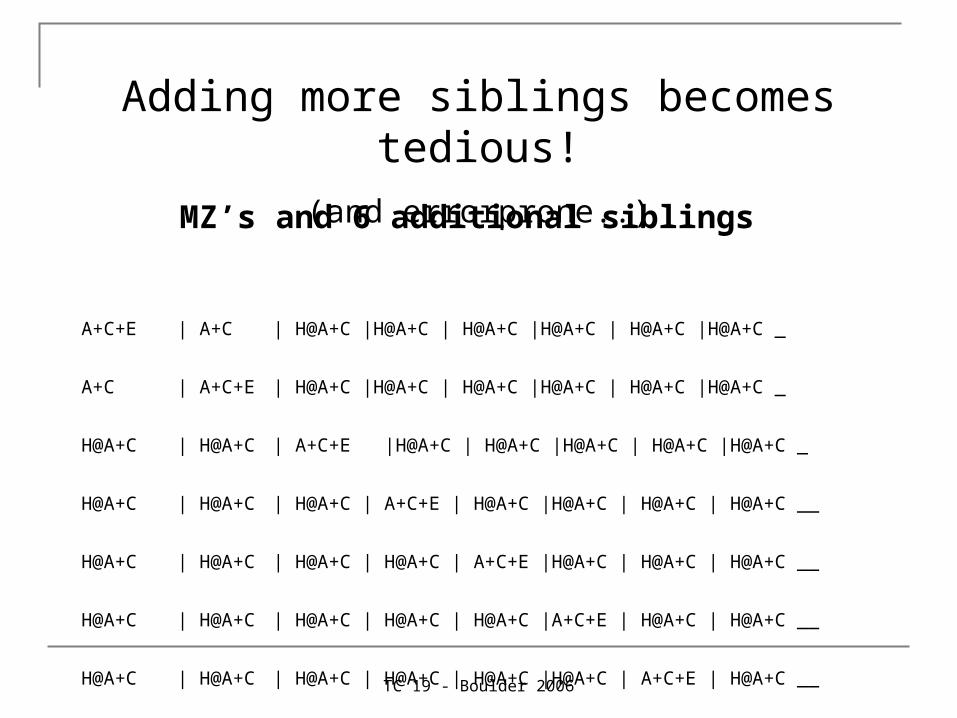
Adding more siblings becomes tedious!
(and errorprone..)
MZ’s and 6 additional siblings
A+C+E | A+C | H@A+C |H@A+C | H@A+C |H@A+C | H@A+C |H@A+C _
A+C | A+C+E | H@A+C |H@A+C | H@A+C |H@A+C | H@A+C |H@A+C _
H@A+C | H@A+C | A+C+E |H@A+C | H@A+C |H@A+C | H@A+C |H@A+C _
H@A+C | H@A+C | H@A+C | A+C+E | H@A+C |H@A+C | H@A+C | H@A+C __
H@A+C | H@A+C | H@A+C | H@A+C | A+C+E |H@A+C | H@A+C | H@A+C __
H@A+C | H@A+C | H@A+C | H@A+C | H@A+C |A+C+E | H@A+C | H@A+C __
H@A+C | H@A+C | H@A+C | H@A+C | H@A+C |H@A+C | A+C+E | H@A+C __
H@A+C | H@A+C | H@A+C | H@A+C | H@A+C |H@A+C | H@A+C | A+C+E ;
TC 19 - Boulder 2006
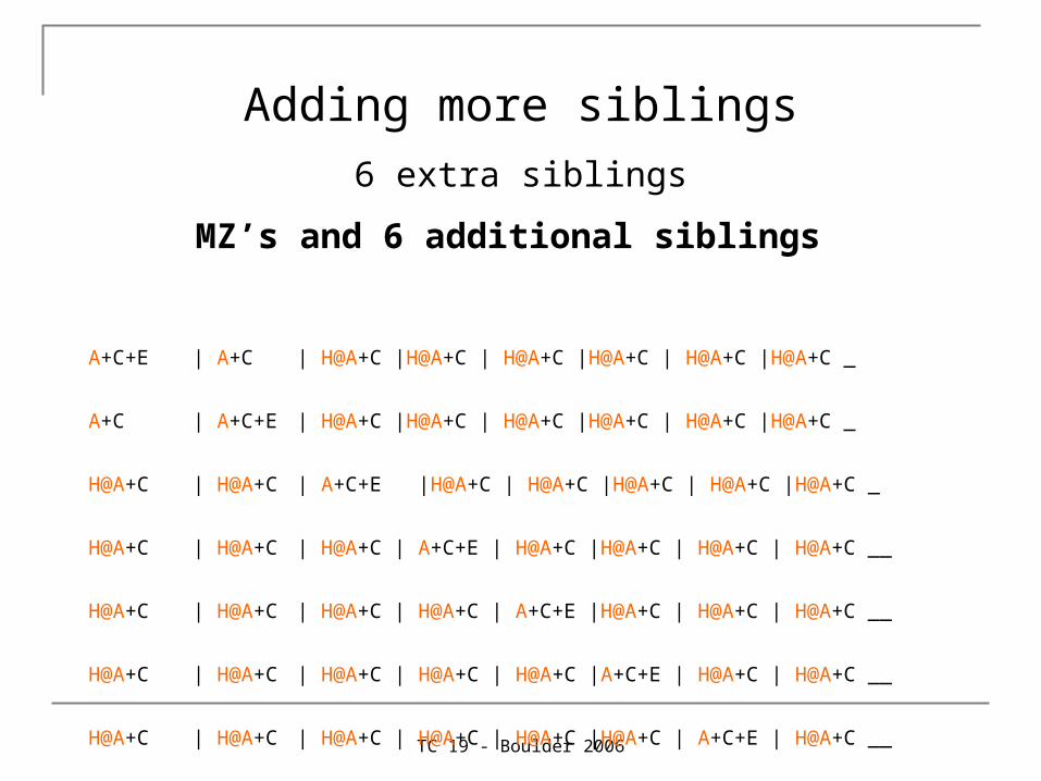
Adding more siblings
6 extra siblings
MZ’s and 6 additional siblings
A+C+E | A+C | H@A+C |H@A+C | H@A+C |H@A+C | H@A+C |H@A+C _
A+C | A+C+E | H@A+C |H@A+C | H@A+C |H@A+C | H@A+C |H@A+C _
H@A+C | H@A+C | A+C+E |H@A+C | H@A+C |H@A+C | H@A+C |H@A+C _
H@A+C | H@A+C | H@A+C | A+C+E | H@A+C |H@A+C | H@A+C | H@A+C __
H@A+C | H@A+C | H@A+C | H@A+C | A+C+E |H@A+C | H@A+C | H@A+C __
H@A+C | H@A+C | H@A+C | H@A+C | H@A+C |A+C+E | H@A+C | H@A+C __
H@A+C | H@A+C | H@A+C | H@A+C | H@A+C |H@A+C | A+C+E | H@A+C __
H@A+C | H@A+C | H@A+C | H@A+C | H@A+C |H@A+C | H@A+C | A+C+E ;
TC 19 - Boulder 2006
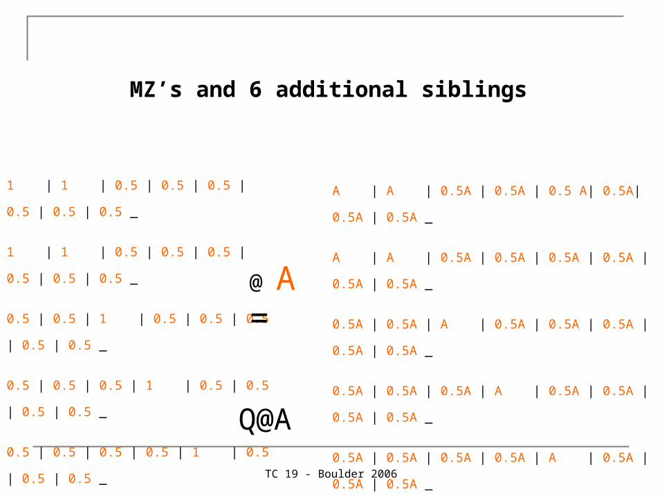
MZ’s and 6 additional siblings
1 | 1 | 0.5 | 0.5 | 0.5 | 0.5 | 0.5 | 0.5 _
1 | 1 | 0.5 | 0.5 | 0.5 | 0.5 | 0.5 | 0.5 _
0.5 | 0.5 | 1 | 0.5 | 0.5 | 0.5 | 0.5 | 0.5 _
0.5 | 0.5 | 0.5 | 1 | 0.5 | 0.5 | 0.5 | 0.5 _
0.5 | 0.5 | 0.5 | 0.5 | 1 | 0.5 | 0.5 | 0.5 _
0.5 | 0.5 | 0.5 | 0.5 | 0.5 |1 | 0.5 | 0.5 _
0.5 | 0.5 | 0.5 | 0.5 | 0.5 | 0.5 | 1 | 0.5 _
0.5 | 0.5 | 0.5 | 0.5 | 0.5 | 0.5 | 0.5 | 1 ;
@ A =
A | A | 0.5A | 0.5A | 0.5 A| 0.5A| 0.5A | 0.5A _
A | A | 0.5A | 0.5A | 0.5A | 0.5A | 0.5A | 0.5A _
0.5A | 0.5A | A | 0.5A | 0.5A | 0.5A | 0.5A | 0.5A _
0.5A | 0.5A | 0.5A | A | 0.5A | 0.5A | 0.5A | 0.5A _
0.5A | 0.5A | 0.5A | 0.5A | A | 0.5A | 0.5A | 0.5A _
0.5A | 0.5A | 0.5A | 0.5A | 0.5A |A | 0.5A | 0.5A _
0.5A | 0.5A | 0.5A | 0.5A | 0.5A | 0.5A | A | 0.5A _
0.5A | 0.5A | 0.5A | 0.5A | 0.5A | 0.5A | 0.5A | A ;
Q@A
TC 19 - Boulder 2006
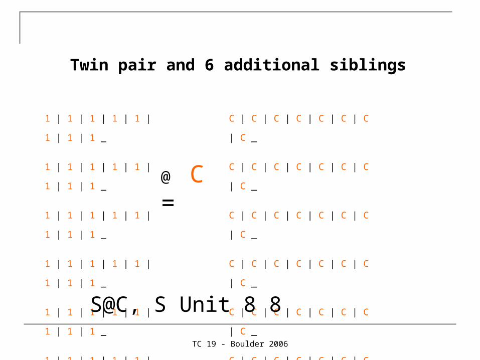
Twin pair and 6 additional siblings
1 | 1 | 1 | 1 | 1 | 1 | 1 | 1 _
1 | 1 | 1 | 1 | 1 | 1 | 1 | 1 _
1 | 1 | 1 | 1 | 1 | 1 | 1 | 1 _
1 | 1 | 1 | 1 | 1 | 1 | 1 | 1 _
1 | 1 | 1 | 1 | 1 | 1 | 1 | 1 _
1 | 1 | 1 | 1 | 1 | 1 | 1 | 1 _
1 | 1 | 1 | 1 | 1 | 1 | 1 | 1 _
1 | 1 | 1 | 1 | 1 | 1 | 1 | 1 ;
@ C =
C | C | C | C | C | C | C | C _
C | C | C | C | C | C | C | C _
C | C | C | C | C | C | C | C _
C | C | C | C | C | C | C | C _
C | C | C | C | C | C | C | C _
C | C | C | C | C | C | C | C _
C | C | C | C | C | C | C | C _
C | C | C | C | C | C | C | C ;
S@C, S Unit 8 8
TC 19 - Boulder 2006
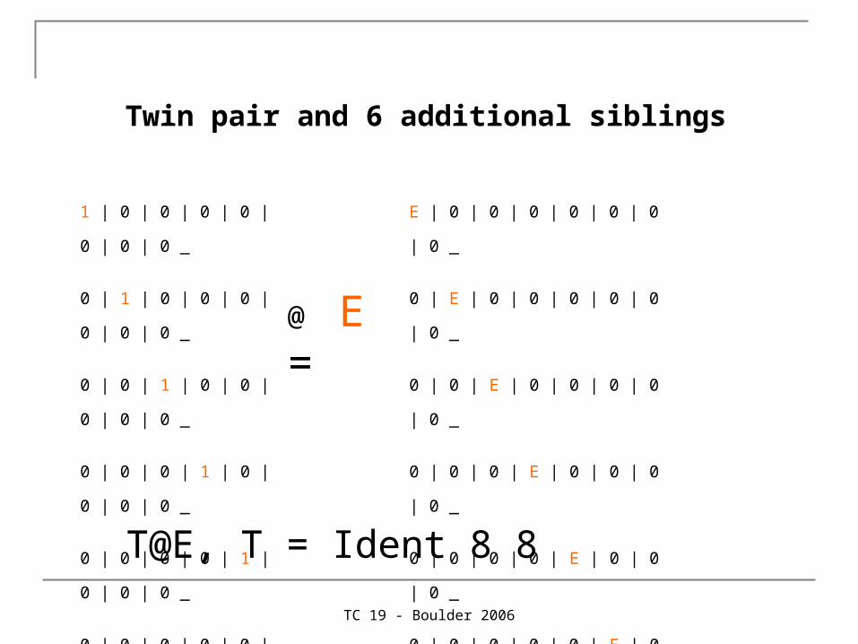
Twin pair and 6 additional siblings
1 | 0 | 0 | 0 | 0 | 0 | 0 | 0 _
0 | 1 | 0 | 0 | 0 | 0 | 0 | 0 _
0 | 0 | 1 | 0 | 0 | 0 | 0 | 0 _
0 | 0 | 0 | 1 | 0 | 0 | 0 | 0 _
0 | 0 | 0 | 0 | 1 | 0 | 0 | 0 _
0 | 0 | 0 | 0 | 0 | 1 | 0 | 0 _
0 | 0 | 0 | 0 | 0 | 0 | 1 | 0 _
0 | 0 | 0 | 0 | 0 | 0 | 0 | 1 ;
@ E =
E | 0 | 0 | 0 | 0 | 0 | 0 | 0 _
0 | E | 0 | 0 | 0 | 0 | 0 | 0 _
0 | 0 | E | 0 | 0 | 0 | 0 | 0 _
0 | 0 | 0 | E | 0 | 0 | 0 | 0 _
0 | 0 | 0 | 0 | E | 0 | 0 | 0 _
0 | 0 | 0 | 0 | 0 | E | 0 | 0 _
0 | 0 | 0 | 0 | 0 | 0 | E | 0 _
0 | 0 | 0 | 0 | 0 | 0 | 0 | E ;
T@E, T = Ident 8 8
TC 19 - Boulder 2006
.
Mx
Copy Twins&6.mx Open Twins&6.mx
TC 19 - Boulder 2006
.
Exercise
Modify this script for maximum nr of siblings = 3, 4, or 5, write down –2ll, df, estimated pms, n observations for each model
TC 19 - Boulder 2006
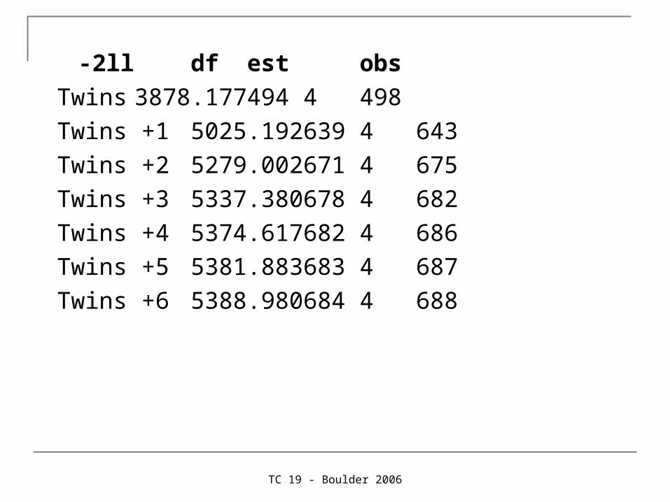
-2ll df est obs
Twins 3878.177 494 4 498
Twins +1 5025.192 639 4 643
Twins +2 5279.002 671 4 675
Twins +3 5337.380 678 4 682
Twins +4 5374.617 682 4 686
Twins +5 5381.883 683 4 687
Twins +6 5388.980 684 4 688
TC 19 - Boulder 2006
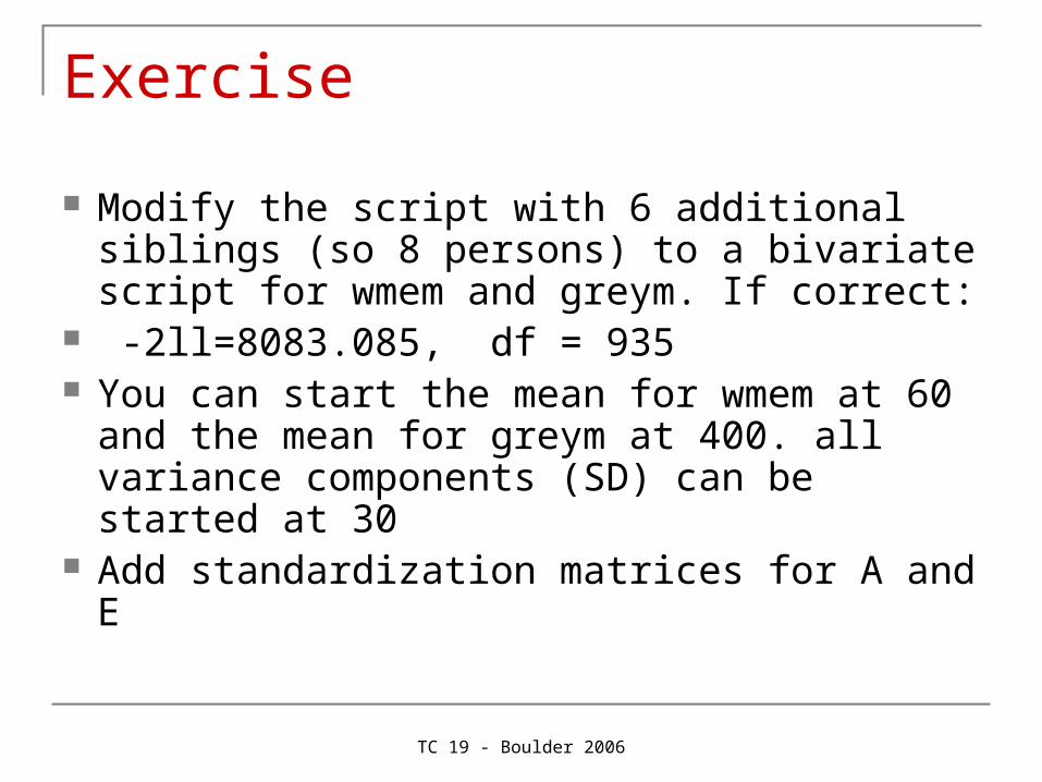
Exercise
Modify the script with 6 additional siblings (so 8 persons) to a bivariate script for wmem and greym. If correct:
-2ll=8083.085, df = 935 You can start the mean for wmem at 60 and
the mean for greym at 400. all variance components (SD) can be started at 30
Add standardization matrices for A and E
TC 19 - Boulder 2006
In Summary
Be aware of assumptions of the twin design
Adding additional persons: add expectations to Covariance statement
Adding additional phenotypes: change matrix dimensions