exposing computer generated images by using deep

Exposing Computer Generated Images by Using

Deep Convolutional Neural Networks

Edmar R. S. de Rezendea, Guilherme C. S. Rupperta, Antonio Theophiloa,Tiago Carvalhob

aCTI Renato Archer, Campinas-SP, Brazil 13069-901bFederal Institute of Sao Paulo (IFSP), Campinas-SP, Brazil 13069-901

Abstract

The recent computer graphics developments have upraised the quality of thegenerated digital content, astonishing the most skeptical viewer. Games andmovies have taken advantage of this fact but, at the same time, these ad-vances have brought serious negative impacts like the ones yielded by fakeimages produced with malicious intents. Digital artists can compose artificialimages capable of deceiving the great majority of people, turning this into avery dangerous weapon in a timespan currently know as “Fake News/Post-Truth” Era. In this work, we propose a new approach for dealing with theproblem of detecting computer generated images, through the application ofdeep convolutional networks and transfer learning techniques. We start fromResidual Networks and develop different models adapted to the binary prob-lem of identifying if an image was or not computer generated. Differentlyfrom the current state-of-the-art approaches, we don’t rely on hand-craftedfeatures, but provide to the model the raw pixel information, achieving thesame 0.97 of state-of-the-art methods with two main advantages: our meth-ods show more stable results (depicted by lower variance) and eliminate thelaborious and manual step of specialized features extraction and selection.

Keywords: digital forensics, CG detection, deep learning, transfer learning,fake news

Preprint submitted to Signal Processing: Image Communication November 29, 2017

arX

iv:1

711.

1039

4v1

[cs

.CV

] 2

8 N

ov 2

017

1. Introduction

The 2016 Global Games Market Report1 presented the economic potentialof digital games, which traded more than 99.6 billions of dollars, an incrementof 8% when compared to the previous year. The growth in this market alwayspushes forward the quality and development of associated industries andtechnologies as, for example, computer graphics methods. These methodsare essential to make games more realistic through high quality graphics.

Another entertainment field that takes advantage of advanced computergraphics methods is the movies industry. Thinking about realism, in thelast years we’ve experienced huge steps towards a complete deceiving of ourvisual senses. Productions as Rogue One: A Star Wars Story showed thepotential of Computer Graphics (CG) characters construction, introducingin a live action movie characters entirely based on real actors.

The search for a perfect generation of digital scenarios, objects and evenpeople is endless and recently reached an astonishing point, mostly helpedwith the latest advances of computing processing, in special the modernGPU cards (Graphics Processing Units). One current example of such anachievement was the digital reproduction of the actress Carrie Fisher in thelast Star Wars movie 2, with the same appearance of the beginning of hercareer in the 70’s.

In spite of the safe and benign results of these advances, once the goal ofperfect CG image generation is accomplished, some threats come along andintroduce new challenges to other science areas as pointed out by Holmeset al. [1]. One example of such a challenge is the identification if an imagewas a photo generated (PG - the one generated by a digital camera) orgenerated by CG methods. Figure 1, shows an example of how difficult is todiscern between PG and CG images.

Recent studies showed how easy is to deceive people using images [2]. Inspecial, several examples of undesired situations can be described involvingthe CG images. Imagine, for example, a CG image depicting a terrorist ex-ecution of a kidnapped report spreading across the globe. Or another CGimage of a rising politician, posted in social networks putting him in an em-barrassing or criminal situation days before an election. We are living in whatsome are calling the Fake News/Post-Truth Era [3, 4], where mass commu-

1https://goo.gl/xkWPon2http://www.imdb.com/title/tt3748528/

2

(a) PG (b) CG

Figure 1: Example of how challenging is to recognize PG and CG images by simple visualanalysis.

nication platforms (as social media networks) can be used to influence anddeceive people [5, 6]. If a well-crafted invented text can have a great impacton people’s public opinion, imagine the effects of a CG image produced by avery (probably well-paid) skilled professional posted on social networks.

The distinction between PG and CG has even more complex legal im-plications when related to child pornography. In Brazil, any person whoproduces, reproduces, directs, takes pictures or records, in any way, scenesinvolving explicit sexual or pornographic act involving children or teenager,can be sued according to Brazilian Law 11,829 published on November 25th,2008. This legal process can result in 4 to 8 years in jail. This situationraises a fundamental legal and ethical question created by technology: Whathappens if the material is proved to be CG generated? Are the legal conse-quences the same?

The task of CG image and video detection was already studied and severalDigital Forensics methods were proposed [7, 8, 9, 10]. However, the resultsare far from considering the problem as completely solved. Very often these

3

methods are based on the discovery of inconsistencies in very specific situ-ations, hindering their wide application. For example, Conotter et al. [11]developed a method based on blood flow information of CG constructed peo-ple in videos. In contrast, Tokuda et al. [7] proposed a more generic methodthat applies machine learning techniques to solve the CG image identificationtask and is more similar with the one presented by this work.

The rise of Deep Neural Networks (DNN) in the past few years, presenteda shift in classification process, specially in the feature engineering step of thisprocess. Algorithms based on DNN have outperformed other approaches inimage classification, becoming the standard approach for these tasks. Theyconsist of learning algorithms with multiple levels, acting over the raw input(image pixels for example) transforming the representation at one level intoa representation at a higher, slightly-more-abstract level [12, 13, 14]. Asthis stack of layers gets bigger, more complex functions can be learned fromdata. Besides this power of representing more complicated mappings, a greatadvantage of DNN is that there is no need for human engineered features,with a general purpose algorithm learning direct from raw data.

In spite of the basic concepts of DNN being around for some decades,only now, with the plenty availability of data and the recent developments ofGPU cards, DNN showed its full potential, specially in image classificationchallenges such as the ILSVRC (ImageNet Large Scale Visual RecognitionChallenge) [15]. This highlighted the transition from hand-crafted featurescombined with shallow classifiers to deep classifiers acting directly on rawdata as is the case of DNNs.

Since then, there is been a trend of, as deeper the model is, the bet-ter its performance and more difficult is the training process. This can bedemonstrated by ImageNet challenge results. In 2012 the 8-layers AlexNetnetwork [16] astonished the machine learning community winning the chal-lenge with a top-5 classification error rate of 16.4% and a huge leap fromthe second place (this one using usually hand-crafted features and shallowclassifiers). In 2014, two VGG DNN models (one with 16 layers and theother with 19 layers) got a top-5 classification error rate of 7.3% [17] whileGoogleNet with its 22 layers won the challenge with 6.7% error rate [18].Finally, in 2015 the Residual Network (ResNet) model, a DNN with 152 lay-ers, achieved a top-5 classification error of 3.57% [19]. Also, in 2015, for thefirst time, was presented a DNN technique capable of performing better thanhumans in image classification tests [20].

This paper presents a novel approach for dealing with the task of de-

4

tecting CG image generation. Two different models are developed, startingfrom the DNN ResNet with 50 layers (ResNet-50) [19] and adapting it to thebinary problem of CG image detection. Applying concepts of transfer learn-ing [21], we were able to transfer the weights of ResNet-50 layers pre-trainedon ImageNet dataset to our model, avoiding overfitting and achieving 97%of accuracy without the burden of designing complex hand-craft features. Toour best knowledge, this is the first work to propose applying DNN techniquesto this problem, not requiring human experts to design features.

Regarding the actual state-of-the-art method for detection of CG imagegeneration [7], the main contributions of this paper are: (1) the proposal of anew approach based on DNN and transfer learning techniques that achievesthe same accuracy of 0.97 as state-of-the-art methods without the need forhuman level feature extraction; (2) the use of an extended dataset (moredifficult for the task); (3) a more stable method proved by the lower varianceresults3; (4) evaluation of different kinds of classifiers in association with aDNN in order to find the best combination (features + classifier); (5) anda qualitative analysis of bottleneck features produced by ResNet-50 in CGimage detection problem.

The text is structured in the following way: Section 2 briefly presents themain works in the Digital Forensics literature that deal with the problem ofdetecting CG image generation. Section 3 explains with details the proposedmethodology while Section 4 describes the main experiments conducted tovalidate the methodology and presents the achieved results, comparing withthe state-of-the-art found on the literature. Lastly, Section 5 presents themain conclusions and some future research directions.

2. Related Work

There are many works in the literature on the topic of distinguishingbetween CG and real images. Holmes et.al. [1] discusses the legal aspectsrelated to the problem, specially for child pornography. The authors inves-tigated the perception of humans exposed to this kind of image performingtwo experiments: (i) the first one in which a set of images (CG and real)are shown to untrained users, and (ii) the second where there was a previoustraining for users before showing the images. The experiment consisted in

3All the artifacts (code and dataset) produced by this work will be available in case ofpaper acceptance.

5

submitting each user to 60 pictures of people. The user were asked to identifythe sex (man or woman) and if the image was real or generated by computer.In the first round of experiments, the untrained users achieved an accuracyaround 50% in CG image detection. In the second experiment, after a sim-ple training, the users improved their accuracy at the task. Also, as the CGimage quality improves, it becomes even easier to trick the perception of theuser to distinguish real and CG images.

The work [22] discusses the US Supreme Court decision on not consid-ering as a crime the computer generated child pornography. Also, the workpresents techniques for image tampering and approaches to detect some kindsof image manipulation.

Conotter et.al. [11] proposed to use information associated with bloodflow and perceptual details to detect computer generated people in videos.The method consists in evaluating small movements of cheeks and foreheadto generate a distinguishable signal of CG and real images. This signal ismore stable for real images, while CG images present many peaks.

Many methods based on machine learning have been proposed, whichtypically consists in extracting features and using a supervised learning clas-sifier to identify patterns of CG or real images. Tokuda et.al. [7] proposesa method using fusion of many classifiers combined with a big number offeature extraction schemes, achieving a 97% accuracy on his dataset (9700images).

Tan et.al. [23] uses Local Ternary Patterns (LTP) for features extraction,and rely only on texture features to distinguish CG and real images. Exper-iments reveal that the method achieves an accuracy of approximately 97%in a dataset of 2200 images collected from different sources, as for example,the Columbia University natural image library [24],using a Support VectorMachine (SVM) [25] classifier.

3. Proposed Method

The CG detection method proposed in this work relies upon a deep CNNarchitecture to classify each image from the dataset using the raw RGB pixelsvalues as features, without the need for manual feature extraction. The deepCNN deployed is based on the ResNet-50 model [19] and the method usestransfer learning techniques [21]. All the pipeline of proposed method asfundamental concepts related with it will be explained in the next sections.

6

3.1. Complete Model Architecture

Our proposed deep CNN model uses transfer learning techniques, lever-aging the outcomes of residual learning presented by He et al. [19]. The finalmodel architecture, with its pipeline depicted in Figure 2, consists of:

1. an initial pre-processing stage;

2. a sequence of many convolutional layers based on the first 49 layers ofResNet-50 and;

3. a top classifier replacing the original 1000 fully-connected softmax layer.

Test Image

(F1, F2, F3, … , Fn-2, Fn-1, Fn, ?)

?Classifier

CG Detection

Pre-processing

BottleneckFeaturesExtractor

7x7 conv, 64, /2

3x3 max pool, /2

3x1x1 conv, 643x3 conv, 641x1 conv, 256




avg. pool

1000 fc, softmax

ResNet-50


Pre-processing

Training Set

PG ImagesCG Images


(F1, F2, F3, … , Fn-2, Fn-1, Fn, CG1)...

(F1, F2, F3, … , Fn-2, Fn-1, Fn, CGN)(F1, F2, F3, … , Fn-2, Fn-1, Fn, PG1)...

(F1, F2, F3, … , Fn-2, Fn-1, Fn, PGN)

Bottleneck Features

Training

CG Images PG Images

Pre-processed Images

TransferLearning

Figure 2: Overview of proposed method. Transferring ResNet-50 parameters to our modelto extract bottleneck features, which are used to train different classifiers.

In a real word dataset, images can present different resolutions. However,our model requires a constant input dimensionality. Therefore, we resize theimages to a fixed resolution of 224 × 224 and, for each pixel, we subtractthe mean RGB value computed over the ImageNet dataset (as proposed byKrizhevsky et al. [16]). These two operations are performed by the pre-processing layer.

After pre-processing the dataset images, we apply the transfer learningtechniques explained in Section 3.3. In our CNN model, after the pre-processing, we use the first 49 layers of ResNet-50 with their weights trained

7

on ImageNet as a features extractor (red box named “Bottleneck FeaturesExtractor” of Figure 2) to generate a set of features with the correspondentlabel associated. These labelled features, also called bottleneck features4 arethe activation maps generated by the average pooling layer (the 49th layer ofResNet-50), ignoring the last 1000 fully-connected softmax layer.

These bottleneck features are used to train a top classifier that will makethe final prediction of CG images. This classifier has the same role as theoriginal softmax layer at the end of ResNet-50, adapting the network to thebinary problem of CG image detection. The replacement of this softmaxlayer, with thousands of parameters, associated with the transfer learningtechniques used (no learning happens at the convolutional layers), allowedus to deploy a very deep CNN for the CG image detection problem withoutthe requirement of millions of CG/PG labelled images, besides significantlyreducing the training time.

Once finished the training process, our final deep CNN model used fortesting is made up of the pre-processing layer, the Bottleneck Features Ex-tractor and a top classifier (network on the right of Figure 2). Different typeof classifiers were trained as top predictors in order to discover which oneperforms best for the task of CG image detection. Section 3.4 will delve intothe details of each type used.

3.2. ResNet-50

Residual Networks (ResNet) [19] can be classified as convolutional neuralnetworks (CNN). These CNNs, in turn, can be defined as neural networksthat have at least one layer using the convolution operation [13]. Mathemat-ically speaking, the convolution operation can be view as a weighted averageoperation of two functions (x and w), where one of them (w) is a probabilitydensity function. More formally:

s(t) = (x ∗ w)(t) =∫x(a)w(t− a)da (1)

4Bottleneck term refers to a neural network topology where the hidden layer has signif-icantly lower dimensionality than the input layer, assuming that such layer — referred toas the bottleneck — compresses the information needed for mapping the neural networkinput to the neural network output, increasing the system robustness to noise and over-fitting. Conventionally, bottleneck features are the output generated by the bottlenecklayer.

8

In practice, due to the commutative property, the convolution operationis usually implemented as the cross-correlation function [13]. For example,assuming the function x as a two-dimensional input image I and the proba-bility density function w as a function K (usually called kernel in machinelearning terminology), the function S below is the convolution of kernel Kover the image I:

S(i, j) = (I ∗K)(i, j) =∑m

∑n

I(i+m, j + n)K(m,n) (2)

In machine learning nomenclature, the function S is usually called a fea-ture map. Among many interesting properties that convolutions convey, oneof paramount importance is the robustness to translation in the recognitionof patterns. If a kernel K is specialized in recognizing circles, the convolutionof this kernel over the image will identify circles no matter where they occurin the image.

Besides convolutions, CNNs usually have some non-linear activation func-tions (like sigmoid or rectified linear functions) and pooling layers that havethe effect of turning the representation invariant to small translations in theimage [13].

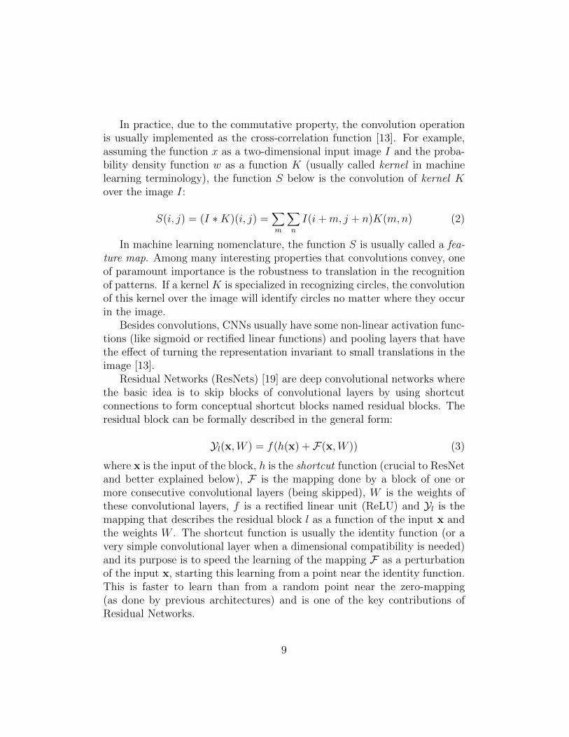
Residual Networks (ResNets) [19] are deep convolutional networks wherethe basic idea is to skip blocks of convolutional layers by using shortcutconnections to form conceptual shortcut blocks named residual blocks. Theresidual block can be formally described in the general form:

Yl(x,W ) = f(h(x) + F(x,W )) (3)

where x is the input of the block, h is the shortcut function (crucial to ResNetand better explained below), F is the mapping done by a block of one ormore consecutive convolutional layers (being skipped), W is the weights ofthese convolutional layers, f is a rectified linear unit (ReLU) and Yl is themapping that describes the residual block l as a function of the input x andthe weights W . The shortcut function is usually the identity function (or avery simple convolutional layer when a dimensional compatibility is needed)and its purpose is to speed the learning of the mapping F as a perturbationof the input x, starting this learning from a point near the identity function.This is faster to learn than from a random point near the zero-mapping(as done by previous architectures) and is one of the key contributions ofResidual Networks.

9

In ResNet-50 architecture, the basic residual blocks, also called bottle-neck blocks, are composed of a sequence of three convolutional layers withfilters of size 1 × 1, 3 × 3 and 1 × 1 respectively. The down-sampling isperformed directly by convolutional layers that have a stride of 2 and batchnormalization [26] is performed right after each convolution and before ReLUactivation.

The identity shortcuts can be directly used when the input and outputfeature maps are of the same dimensions. When the dimensions change,two options are considered: (i) The shortcut still performs identity mapping,with extra zero entries padded for increasing filter dimensions (depth). Thisoption introduces no extra parameter; (ii) A 1×1 convolution layer is used tomatch the dimensions. This is called projection shortcut. For both options,when the shortcuts go across feature maps of two sizes, they are performedwith a stride of 2. Figure 3 tries to clarify this set-up.

1x1 conv, 4f

BN

input

1x1 conv, f

3x3 conv, f

1x1 conv, 4f

+

BNReLU

ReLU

BNReLU

BN

input

1x1 conv, f

3x3 conv, f

1x1 conv, 4f

+

BNReLU

ReLU

BNReLU

BN

Figure 3: Bottleneck Blocks for ResNet-50 (left: identity shortcut; right: projection short-cut).

The network ends with a global average pooling layer and a 1000-wayfully-connected layer with softmax activation. The total number of weightedlayers is 50.

3.3. Transfer Learning

Deep learning techniques usually require a very large number of samplesand demands a heavy computing effort. In this scenario, transfer learning

10

[21] has gained a lot of attention. It represents the possibility to transferthe knowledge learned from one problem to another problem. For neuralnetworks, the transfer learning process consists, in practice, in transferringthe parameters of a (source) neural network that was previously trained fora particular dataset for a specific task to another (target) network with adifferent dataset to solve a different problem.

A typical transfer learning procedure implies in using an already trainedbase network and copying all the parameters from the first n layers to thefirst n layers of the target network. Then, a supervised training is performedonly on the remaining layers that were not copied. Since the task is differentand probably so is number of classes, the last layer has to be modified tocontain the same amount of neuron as the number of classes or it can bereplaced by another classifier. During this training, the copied layers can beleft fixed, or it can fine-tuned by allowing the backpropagation process intothe copies parameters. Usually fine-tuning improves the accuracy, however,when the number of parameters is big and the numbers of samples is small,this may result in overfitting and fine-tuning should not be used.

In traditional supervised learning, the common sense was settled thatthe training should always be performed specifically for a given task anddataset and the transfer learning approach could sound senseless. However,in general, deep neural networks present a particular characteristic which isto learn features in the first layers that are more general and not specific tothat particular dataset and problem. That makes that knowledge reusablefor other problems and dataset. On the other hand, the knowledge learnedon the last layers of the neural network are more specific for that task.

Transfer learning is very handy because it avoids the task of trainingthe network. Since the architecture is very deep, training it represents anenormous computational efforts requiring expensive high processing comput-ers, usually using multiple high-end GPU units. Another problem in trainingdeep networks from scratch is that it required a vary large number of samples,otherwise is will overfit the data. Transfer learning significantly mitigates thistwo problems, enabling the use of deep learning even when the target datasetis small or when there is limited computing resources. Recent studies havetaken advantage of this fact to obtain state-of-the-art results [27][28][29],which evidences the generality of the features learned in the first layers ofthe network.

In this work, we apply transfer learning technique by using the sameparameters of the ResNet-50 network trained for the ImageNet 2012 compe-

11

tition [15] which provided a 1.28 million images dataset from 1000 classes.The first 49 layers of the network were copied to a new ResNet-50 networkand we removed the last layer, replacing it by another classifier. We havenot used fine-tuning during the training due to the relatively small dataset.

3.4. Top Classifier

In the proposed method, the last layer of the ResNet-50 is replaced byanother classifier and we have evaluated four different classifier for this task.

3.4.1. Softmax

The softmax function[25] is widely used in deep learning architecturesand consists in the generalization of the binary logistic regression to multipleclasses.

This function is particularly interesting because it provides an intuitiveoutput with probabilist interpretation. The outcome of the function is avector containing the probability for each class.

Typically, the softmax is used for classification as the activation functionon the last fully-connected layer of CNNs, which is the case in the ResNet-50.The function transforms a vector z with dimension K of real numbers zk, toanother vector σ(z) of same dimensions with the values ranging from 0 to 1.The sum of the output vector adds up to 1, therefore it can be interpretedas the probabilities for each class. The formula is given by:

σ(z)j =ezj∑Kk=1 ezk

(4)

For training, we used the categorical cross-entropy loss function, which isgiven by:

H(p, q) = −∑x

p(x).log(q(x)) (5)

3.4.2. k-Nearest Neighbor (kNN)

The k-Nearest Neighbor (kNN) [25] classifier is one of the simplest andmost popular supervised classifier. It consists in classifying a sample based onthe k nearest samples from the training set. Usually, the euclidean distancefunction is used, but other distance functions may be chosen. The sampleis then classified by the majority voting or other similar function among thek nearest samples. The advantage of kNN is that it is very simple, does

12

not require an explicit training step and yet it is very effective for manyapplications, specially when the training set is large. The main drawbacks ofthis method are that (i) the method requires the distance computation to allsamples from the training dataset, which makes it computationally heavy;and (ii) the fact that it also requires a lot of memory since the whole datasethas to be loaded for comparison.

3.4.3. XGBoost

Extreme Gradient Boosting (XGBoost) [30] is a recent work that has beengaining a lot of attention for impressive results in machine learning challengeslike KDD Cup and Kaggle competitions.

XGboost consists of an open-source package that implements gradienttree boosting algorithm with the focus on being highly effective and scal-able. It includes novel optimized algorithms related to: more efficient par-allelization; a novel sparse-aware tree learning algorithm; out-of-core com-putation, cache-aware access; distributed weighted quantile sketch method;among other improvements. All these improvements allow the system toperform more than ten times faster than other tree boosting solutions.

The library was written in C++, however binding for other languages likepython, R and Java are available.

3.4.4. SVM

Support Vector Machines (SVM)[25] is one of the most popular supervisedclassifier and basically operates by finding the optimum hyperplane that bestseparates two classes. Originally designed for binary classification, it can beextended for multi-class problems by reducing one multi-class task to multiplebinary classification problems using techniques known as one-versus-one orone-versus-all, among other methods.

Although the original SVM is a linear classifier, it can be applied for non-linear problems by using kernel functions which nonlinearly maps the featurevector to a new space.

In the present work, we evaluate both the linear SVM and the SVM with aRadial Basis Function (RBF) kernel, for the top classifier of the architecture.

4. Experiments and Results

To validate the proposed approach, we have performed different roundsof experiments which will be detailed in the next sections.

13

4.1. DSTok Dataset

The first dataset in which the proposed method has been tested is a publicdataset proposed by Tokuda et al. [7]. It comprises 4,850 CG images and4,850 PG images, depicting different kinds of scenarios as people, outdoor,objects, cars, animals, and others. The entire set of images has been collectedfrom Internet and compressed in JPEG format, presenting images with sizesfrom 12 KB to 1.8 MB. Images in the dataset present different resolutionsand, differently from Tokuda et al., our proposed method works with theentire image (without cropping). Figure 4 depicts some examples of imagesin DSTok dataset.

(a) CG (b) CG

(c) PG (d) PG

Figure 4: Examples of images in DSTok dataset.

4.2. DSTokExt Dataset

The second dataset used to validate the method is an extension of Tokudaet al. [7] dataset. It comprises 8,394 CG images and 8,002 PG images, also

14

depicting different kinds of scenario. In the same way as Tokuda et al. [7],all the images have been collected from Internet and compressed in JPEGformat, presenting images with sizes from 12 KB to 1.8 MB. Images in thedataset present different resolutions. Figure 5 depicts some examples of im-ages in DSTok dataset.

(a) CG (b) CG

(c) PG (d) PG

Figure 5: Examples of images in DSTokExt dataset.

4.3. Validation Protocol

In order to compare the results achieved by the proposed method withthe results reported by Tokuda et.al. [7], we perform the same five fold cross-validation protocol, reporting the accuracy by fold and the average accuracyfor each round of experiments.

15

4.4. Implementation Details

The proposed methods have been implemented using Python 3.5, Keras2.0.35, and TensorFlow 1.0.16. All performed tests have been executed ina machine with an Intel(R) Xeon(R) CPU E5-2620 2.00GHz processor with96GB of RAM and two Nvidia Titan Xp GPUs.

4.5. Round #1: ResNet-50 trained from Glorot uniform initialization overDSTok

In the first round of experiments we classify samples from DSTok usinga deep CNN architecture similar to the original ResNet-50. Since we haveonly 2 classes (CG and PG), we have adapted the ResNet-50 architectureto the CG detection task replacing its last 1,000 fully-connected softmaxlayer by a 2 fully-connected softmax layer. The weights of the network havebeen initialized using Glorot uniform approach [31] and the bias terms wereinitialized to zero. All layers of the model have been trained for 200 epochswith categorical cross-entropy cost function and Adam optimizer (lr = 0.001,beta1 = 0.9, beta2 = 0.999, epsilon = 1e− 08 and decay = 0.0).

Figures 6 and 7 present, respectively, the average loss and accuracy ofResNet-50 trained from Glorot uniform initialization. Solid lines representthe average performance in the training (red) and testing (green) set whilethe shadows represent the standard deviation in the 5-fold cross-validation.

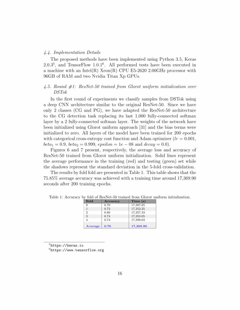
The results by fold fold are presented in Table 1. This table shows that the75.85% average accuracy was achieved with a training time around 17,369.90seconds after 200 training epochs.

Table 1: Accuracy by fold of ResNet-50 trained from Glorot uniform initialization.Fold Accuracy Time (s)0 0.79 17,387.851 0.72 17,352.252 0.80 17,357.333 0.74 17,353.054 0.74 17,399.03

Average 0.76 17,369.90

5https://keras.io6https://www.tensorflow.org

16

Figure 6: Train and test average loss of ResNet-50 trained from Glorot uniform initializa-tion.

4.6. Round #2: ResNet-50 fine-tuned from ImageNet initialization over DSTok

In the second round of experiments, we evaluate the impact of transferlearning as a strategy to initialize the weights of the convolutional layers inthe proposed model. We transfer the weights of ResNet-50 convolutionallayers pre-trained on ImageNet dataset to our deep CNN model, replacingthe last 1000 fully-connected softmax layer by a 2 fully-connected softmaxlayer.

In the first round of experiments, all network parameters (including thelast layer) have been initialized using Glorot uniform approach and the biasterms were initialized to zero. At this round of experiments, we use Ima-geNet parameters as initial weights, except in the last layer where, again, weapply Glorot uniform initialization. Then, all layers have been trained for200 epochs with categorical cross-entropy cost function and Adam optimizer(lr = 0.001, beta1 = 0.9, beta2 = 0.999, epsilon = 1e− 08 and decay = 0.0).

Figures 8 and 9 present, respectively, the average loss and accuracy ofResNet-50 fine-tuned from ImageNet initialization. Solid lines represent theaverage performance in the training (red) and testing (green) set while theshadows represent the standard deviation in the 5-fold cross-validation.

The results by fold are presented in Table 2. This table shows that the82.12% average accuracy was achieved with a training time around 16,889.14seconds after 200 training epochs.

Given the improvement of 7% over the average accuracy obtained in the

17

Figure 7: Train and test average accuracy of ResNet-50 trained from Glorot uniforminitialization.

Table 2: Accuracy by fold of ResNet-50 fine-tuned from ImageNet initialization.Fold Accuracy Time (s)0 0.86 16,888.321 0.82 16,895.002 0.85 16,897.953 0.77 16,879.804 0.80 16,884.62

Average 0.82 16,889.14

experiments of Round #1, we can conclude that the knowledge transferredfrom ImageNet dataset to CG image detection problem produced good re-sults.

4.7. Round #3: ResNet-50 fine-tuned from ImageNet initialization and pre-trained softmax layer over DSTok

In Round #2 of experiments, we showed that the transfer learning in facthelps to improve the model accuracy of CG detection task. However, therandom initialization of the last fully-connected softmax layer could causean undesired drawback backpropagating the error from the last layer to theImageNet transferred weights during the fine-tune step along the entire net-work, degrading the model accuracy.

Therefore, in this round of experiments, we pre-train the last fully-connectedsoftmax layer before the fine-tuning step along the entire network. To per-form this, we initialize the convolutional layers with ImageNet weights and

18

Figure 8: Train and test average loss of ResNet-50 fine-tuned from ImageNet initialization.

freeze them. Then, the weights of the last layer are initialized using Glorotuniform approach, the bias terms are initialized to zero and the network ispre-trained for 200 epochs with categorical cross-entropy cost function andAdam optimizer (lr = 0.001, beta1 = 0.9, beta2 = 0.999, epsilon = 1e − 08and decay = 0.0). This procedure results in the training of the softmaxlayer, only. After this step, we unfreeze convolutional layers, training alllayers of the model for 200 epochs with categorical cross-entropy cost func-tion and SGD optimizer (lr = 0.0001, momentum = 0.9, decay = 0.0 andnesterov = False), using a smaller learning rate to train the network. Sincewe expect the pre-trained weights to be quite good already as compared torandomly initialized weights, we do not want to distort them too quickly andtoo much.

Figures 10 and 11 present, respectively, the average loss and accuracy ofResNet-50 fine-tuned from ImageNet initialization and pre-trained softmaxlayer. Solid lines represent the average performance in the training (red) andtesting (green) set while the shadows represent the standard deviation in the5-fold cross-validation.

The results by fold are presented in Table 3. As can be seen in the table,the 2 fully-connected softmax layer pre-trained with bottleneck features (ob-tained freezing ImageNet weights in convolutional layers) achieved an averageaccuracy of 89.90% after 200 pre-training epochs and the model fine-tunedafter this pre-training step achieved an average accuracy of 91.96% with atraining time around 16,634.51 seconds after 200 training epochs.

19

Figure 9: Train and test average accuracy of ResNet-50 fine-tuned from ImageNet initial-ization.

Table 3: Accuracy by fold of 2 fully-connected softmax layer trained with bottleneckfeatures and ResNet-50 fine-tuned from ImageNet initialization.

Fold Pre-trainAccuracy

ModelAccuracy

Time (s)

0 0.91 0.93 16,716.761 0.89 0.90 16,618.892 0.91 0.92 16,596.873 0.89 0.91 16,620.854 0.90 0.93 16,619.18

Average 0.90 0.92 16,634.51

Those results confirm our hypothesis that, despite the disparity betweenobject detection and CG detection tasks, ResNet-50 comprehensively trainedon the large-scale well-annotated ImageNet may still be transferred to makeCG detection task more effective. Furthermore, it is important to highlightthat ResNet-50 bottleneck features provide a very discriminative image de-scriptor for CG detection problem.

4.8. Round #4: ResNet-50 bottleneck features with Shallow Classifiers overDSTok

Based on the promising results obtained with the knowledge transferof ResNet-50 convolutional layers pre-trained on ImageNet dataset, in thisround of experiments we evaluate the performance of transfer learning com-bined with shallow classifiers.

20

Figure 10: Train and test average loss of ResNet-50 fine-tuned from ImageNet initializationand pre-trained softmax layer.

Therefore, we replace the last fully-connected softmax layer of ResNet-50 by shallow classifiers in order to classify images represented by bottle-neck features. We evaluate the performance of proposed method replac-ing the top layer by three different classifiers: Support Vector Machine(SVM) [25], k-Nearest Neighbor (kNN) [25], and Extreme Gradient Boosting(XGBoost) [30].

For the SVM classifier we use two different kernels: a linear kernel,where the parameter C has been obtained through a grid search process withC ∈ [10−2, 10−1, ..., 1010], and a Radial Basis Function (RBF) kernel, wherethe parameters C and gamma (γ) have been obtained through a gridsearchprocess with C ∈ [10−2, 10−1, ..., 1010] and γ ∈ [10−9, 10−8, ..., 103].

The best C obtained for linear kernel was 0.01 and for RBF kernel thebest C obtained was 10.0 with a γ of 0.001. Figure 12 shows the accuraciesobtained in the gridsearch of parameters C and gamma using RBF kernel.For kNN classifier, we use a k = 1 and for XGBoost the learning rate (lr)was 0.1, maxdepth (md) was 3 and the number of estimators (ne) was 100.

Table 4 summarizes the results for each round of experiments, includingthe shallow classifiers proposed at this round. The best average accuracyachieved was 0.94 using SVM with RBF kernel, with a standard deviation of0.0065 and a variance of 0.00003.

The ROC curve is presented in Figure 13. Additionally, in Figure 14 wealso provide the learning curve for the SVM with RBF Kernel

21

Figure 11: Train and test average accuracy of ResNet-50 fine-tuned from ImageNet ini-tialization and pre-trained softmax layer.

Analyzing the learning curve, it is possible to observe that the trainingscore is around the maximum and the validation score could be increasedwith more training samples. This observation led us to the next round ofexperiments, where we evaluate the transfer learning combined with SVMRBF performance in DSTokExt Dataset, which is an extended version ofDSTok dataset proposed by Tokuda et al. [7].

4.9. Round #5: ResNet-50 bottleneck features with SVM over DSTokExt

The transfer of ResNet-50 convolutional layers trained on ImageNet datasetto CG image detection problem provided results comparable to the best lit-erature methods. Furthermore, as showed in Round #4, the learning curveof ResNet 50 + SVM RBF suggests that increasing the number of samplescould improve the model accuracy.

At this round of experiments, we use an extended version of DSTokdataset, named DSTokExt and described in Section 4.2, to improve meth-ods accuracy. We used the best model (ResNet-50 + SVM RBF) obtainedin Round #4 and performed a gridsearch to find the parameters C andgamma of the SVM RBF classifier with C ∈ [10−2, 10−1, ..., 1010] and γ ∈[10−9, 10−8, ..., 103]. The best C was 10.0 with a γ of 0.001, the same valuesobtained in Round #4. The average accuracy achieved was 0.97 with anstandard deviation of 0.003 and a variance of 6.85E-06. The ROC curve isdepicted in Figure 15. The area under the curve (AUC) is 0.97 and Table 5

22

Figure 12: Gridsearch of parameters C and gamma of SVM with RBF kernel.

Table 4: Summary of proposed approaches along 4 rounds of experiments.Architecture Train Epochs Transfer Avg

AccStdDev

Variance

ResNet-50 +2fc softmax

from scratch 200 no 0.76 0.035 9.81E-04


fine tune 200 yes 0.82 0.035 9.73E-04


pre-train top +fine tune

200 yes 0.92 0.011 9.79E-05

ResNet-50 +kNN

k=1 yes 0.89 0.006 4.41E-05

ResNet-50 +XGBoost

lr=0.1, md=3,ne=100

yes 0.90 0.007 3.56E-05

ResNet-50 +SVM Linear

C=0.01 yes 0.92 0.007 4.39E-04

ResNet-50 +SVM RBF

C=10,γ=0.001

yes 0.94 0.007 3.38E-05

presents the accuracy for each fold.Figure 16 presents the learning curve for this round, with the red curve

representing the training score, green curve representing the average testscore and the green shadow representing the standard deviation across thefolds. Again, as depicted in learning curve of Round #4, it is possible toobserve that the validation score could still be increased with more trainingsamples.

Figure 17 shows a comparison of confusion matrix (left) and the nor-malized confusion matrix (right) obtained with ResNet-50 + SVM RBF onDSTok and DSTokExt datasets.

23

Figure 13: ROC curve for the best result in DSTok dataset using ResNet-50 + SVM RBFKernel.

Table 5: Accuracy by fold of ResNet-50 + SVM RBF over DSTokExt.Fold Accuracy0 0.971 0.982 0.973 0.974 0.96

Average 0.97

4.10. Round #6: Visualization of Bottleneck Features

As described in Section 3, our method takes advantage of transfer learningprocess to generate ResNet-50 bottleneck features, projecting the 150,528input features (224 × 224 × 3 RGB values of the pixels of each image) in alower-dimensional space of 2,048 features. This process intends to generatea set of features with a better degree of separability, which could allow thetop classifier to achieve a higher classification accuracy.

To evaluate if the bottleneck features would, in fact, produce the de-sired boost in classification accuracy, we applied the t-Distributed Stochas-tic Neighbor Embedding (t-SNE) [32] dimensionality reduction technique tovisualize our high-dimensional features. We projected the 150,528 input fea-tures and the 2,048 bottleneck features in 2D, and plot them as points coloredaccording to their class, as depicted in Figure 18 for the images in DSTokdataset and Figure 19 for the images in DSTokExt dataset. Green circles

24

Figure 14: SVM Learning Curve.

represent CG samples while blue squares represent PG samples.It is possible to observe in the figures that the operations performed

by ResNet-50 convolutional layers projected the raw pixels into a betterseparable feature space.

4.11. Round #7:Comparative Analysis

Along five rounds of experiments, we exposed how transfer learning canbe used to take advantage of a DNN trained for object recognition task togenerate discriminative features for CG images. These features can be usedto train accurate classifiers for CG detection problem. The best accuracy of0.97 was achieved using bottleneck features with an SVM classifier with RBFkernel in an extended version of DSTok dataset (containing DSTok imagesplus additional images).

In Tokuda et.al. [7], the authors present an extensive comparison of sev-eral literature approaches dedicated to solve the problem of detecting CGand PG images. The main characteristics of each method investigated bythe authors are reported in Table 6. Additionally, we included the charac-teristics of all methods proposed in this work: (1) ResNet-50 trained fromGlorot uniform initialization (DNN1); (2) ResNet-50 fine-tuned from Ima-geNet initialization (DNN2); (3) ResNet-50 fine-tuned from ImageNet ini-tialization and pre-trained softmax layer (DNN3); (4) ResNet-50 bottleneckfeatures with kNN (DNN4); (5) ResNet-50 bottleneck features with XGBoost

25

Figure 15: ROC curve for the best result in DSTokExt dataset using ResNet-50 + SVMRBF Kernel.

(DNN5); (6) ResNet-50 bottleneck features with SVM Linear (DNN6); and(7) ResNet-50 bottleneck features with SVM RBF (DNN7).

Considering that our experimental protocol is exactly the same one adoptedby Tokuda et.al. [7], we used the results reported by the authors to compareour method with other literature methods. In addition, we also include theresults obtained using the DSTokExt dataset in the comparison table. Ta-ble 7 presents these results. From the table, we see that the accuracies ofliterature methods have a large range of values going from 0.97 (highest)to 0.552 (lowest). Proposed method DNN7 overcome all literature methodsbased on raw and simple features and it is better than FUS1 proposed byTokuda et al. [7]. This fact shows the expression power of transfer learningapproach in features extraction process. Additionally, when DNN7 have thenumber of training samples increased, it achieves the same accuracy as thebest approach proposed by Tokuda et al. [7] but with a lower variance.

In Table 7, it is possible to observe that our method performs better thanthe lowest fusion approach, even using a single kind of feature. Moreover, in-creasing the size of training dataset, our approach presents the same result asthe best fusion proposed by Tokuda et al. [7] with two main advantages: theabsence of laborious hand-craft feature extraction work and a lower variancein results (showing more stability).

26

Figure 16: SVM Learning Curve over DSTokExt dataset.

5. Conclusions and Research Directions

In this paper we have presented a new method for CG images detectionusing a deep convolutional neural network model based on ResNet-50 andtransfer learning concepts. After a simple pre-processing, each image in ourdataset is fed into our deep CNN model and, as result, we obtain a 2048dimension feature vector, here called bottleneck features. Exploring differentapproaches looking for achieving the most effective problem solution, weevaluate different approaches, since train ResNet-50 architecture from scratch(just changing the 1000fc softmax from original architecture to a 2fc softmaxin top layer), using our dataset, for CG detection process, until full transferlearning, where ImageNet weights for ResNet-50 are totally frozen in a wayto produce bottleneck features, which are used to train different machinelearning classifiers to detect if an image is, or not, produced by computergraphics methods.

Conducting different rounds of experiments, we evaluate the efficiencyand effectiveness of using a Deep CNN architecture, proposed for a objectrecognition task, in a CG detection problem, where we are looking for distin-guish between a CG and a PG image, involving different kinds of objects andcontext. Results showed that proposed approach perform as good as state-of-the-art methods in the same dataset, achieving more than 0.97 accuracyrate. These results highlight two main advantages of proposed method: (1)absence of require a hand-craft feature extraction and (2) more stability de-picted by a lower variance.

27

(a) DSTok dataset

(b) DSTokExt dataset

Figure 17: Confusion matrix of the SVM classifier.

In special, in Round #6 of experiments (Section 4.10) we showed forDSTok dataset, using t-SNE dimensionality reduction, the expression powerof bottleneck features generated by ResNet-50 transfer layers, which increasesthe classes separability when compared against raw input features. The samebehavior is kept in DSTokExt with more and different kinds of images.

Furthermore, it is important to realize that, as showed in Section 4.9,even with a extended dataset, the learning curve from the SVM classifierit is still not stable, which suggest that training score is not still aroundthe maximum. Since deep learning models needs an astonishing number ofimages to achieve a satisfactory accuracy, we conclude that keeps increasingthe number of images can leads to an accuracy even better.

A limitation of this method is its difficulty in dealing with CG imageswith a high degree of realism. We conducted an experiment with two datasetsinvolving images very similar and with high degree of realism, one proposedby Holmes et al. [1] and a second one proposed by Carvalho et al. [46]. This

28

(a) Raw image pixels (b) Bottleneck features

Figure 18: t-SNE visualization of DSTok dataset using (a) raw image pixels and (b)ResNet-50 bottleneck features.

left a door open for the improvement of this technique or development of anew one that could cope with this difficult scenario.

As research directions, our propose is explore different architectures bot-tleneck features extraction and perform fusion of these architectures in a wayto construct an ensemble of deep architectures.

Acknowledgments

The authors would like to thank the financial support of IFSP-Campinas,FAPESP (grant 2017/12631-6) and CNPq (grants 302923/2014-4, 313152/2015-2 and 423797/2016-6). We also would like to thank the authors Tokuda et.al. [7]who helped us with dataset acquirement and we gratefully acknowledge thesupport of NVIDIA Corporation with the donation of the GPUs used for thisresearch.

29

(a) Raw image pixels (b) Bottleneck features

Figure 19: t-SNE visualization of DSTokExt dataset using (a) raw image pixels and (b)ResNet-50 bottleneck features.

Table 6: Methods evaluated by Tokuda et.al. [7] and methods proposed here. For each ofone of the methods, it is shown the identifiers, the main concepts and the related featuresused by the methods.

Method Main Concept FeatureLi [33] Second order differences Edges/TextureLSB [34] Camera noise AcquisitionLYU [35] Wavelet transform Edges/TexturePOP [36] Interpolator predictor AcquisitionBOX [37] Boxes counting Auto-similarityCON [38] Contourlet transform Edges/TextureCUR [39] Curvelet transform [39] Edges/TextureGLC [40] Cooccurrence matrix TextureHOG [41] Histogram of oriented grads ShapeHSC [42] Histogram of shearlet coeff CurvesLBP [43] Local binary patterns Edges/TextureSHE [44] Shearlet transform Edges/TextureSOB [45] Sobel operator EdgesFUS1 [7] Concatenation CombinationFUS2 [7] Simple voting CombinationFUS3 [7] Weighted voting CombinationFUS4 [7] Meta-classification CombinationDNN1 Deep CNN + Softmax (from scratch) Raw image pixelsDNN2 Deep CNN transfer + Softmax (from ImageNet weights) Raw image pixelsDNN3 Deep CNN transfer + Softmax (fine-tuning) Raw image pixelsDNN4 Deep CNN transfer + kNN Raw image pixelsDNN5 Deep CNN transfer + XGBoost Raw image pixelsDNN6 Deep CNN transfer + SVM Linear Raw image pixelsDNN7 Deep CNN transfer + SVM RBF Raw image pixels

30

Table 7: Comparison among approaches for distinguishing CGs and PGs. Table is sortedfrom highest to lowest average accuracy. For each of the methods, it is shown the numberof dimensions of the feature space (m), the average accuracy for each class, the varianceand the dataset where the experiments have been performed.

Method m Averageaccuracy

Variance Dataset

DNN7 150528 0.97 6.85E-06 DSTokExtFUS4 13 0.97 6.06E-04 DSTokFUS3 13 0.96 3.86E-04 DSTokFUS2 13 0.95 2.82E-04 DSTokDNN7 150528 0.94 3.38E-05 DSTokFUS1 4011 0.93 9.60E-02 DSTokLi 144 0.93 8.27E-05 DSTokDNN6 150528 0.92 4.39E-04 DSTokDNN3 150528 0.92 9.79E-05 DSTokLYU 216 0.92 2.26E-04 DSTokDNN5 150528 0.90 3.56E-05 DSTokCON 696 0.90 3.03E-04 DSTokDNN4 150528 0.89 4.41E-05 DSTokLBP 78 0.87 3.68E-04 DSTokDNN2 150528 0.82 9.73E-04 DSTokCUR 2328 0.80 9.39E-04 DSTokHSC 96 0.80 6.23E-04 DSTokDNN1 150528 0.76 9.81E-04 DSTokHOG 256 0.74 5.20E-04 DSTokSHE 60 0.71 7.84E-04 DSTokLSB 12 0.66 7.53E-04 DSTokGLC 12 0.63 1,01E-03 DSTokPOP 12 0.57 5.95E-04 DSTokBOX 3 0.55 1.45E-03 DSTokSOB 150 0.55 1,05E-03 DSTok

31

References

References

[1] O. Holmes, M. S. Banks, H. Farid, Assessing and Improving the Iden-tification of Computer-Generated Portraits, ACM TAP 13 (2) (2016)12.

[2] V. Schetinger, M. M. Oliveira, R. da Silva, T. J. Carvalho, Humans areeasily fooled by digital images, Computers & Graphics 68 (SupplementC) (2017) 142 – 151, ISSN 0097-8493, doi:\bibinfo{doi}{https://doi.org/10.1016/j.cag.2017.08.010}, URL http://www.sciencedirect.

com/science/article/pii/S0097849317301450.

[3] K. Schulten, A. C. Brown, Evaluating sources in a ’post-truth’ world:Ideas for teaching and learning about fake news., http://tinyurl.com/h3w7rp8, accessed on November 17th, 2017, 2017.

[4] R. Keyes, The Post-Truth Era: Dishonesty and Deception in Contem-porary Life, St. Martin’s Press, ISBN 9781429976220, 2004.

[5] F. Davey-Attlee, I. Soares, The Fake News Machine. Inside a TownGearing Up for 2020., http://money.cnn.com/interactive/media/

the-macedonia-story/, accessed on November 17th, 2017, 2017.

[6] S. Shane, Mystery of Russian Fake on Facebook Solved, bya Brazilian, https://www.nytimes.com/2017/09/13/us/politics/

russia-facebook-election.html, accessed on November 17th, 2017,2017.

[7] E. Tokuda, H. Pedrini, A. Rocha, Computer generated images vs. digitalphotographs: A synergetic feature and classifier combination approach,Elsevier JVCI 24 (8) (2013) 1276 – 1292.

[8] D. Dang-Nguyen, G. Boato, F. G. B. D. Natale, Discrimination betweencomputer generated and natural human faces based on asymmetry in-formation, in: IEEE EUSIPCO, 1234–1238, 2012.

[9] D. Dang-Nguyen, G. Boato, F. G. B. D. Natale, Identify computergenerated characters by analysing facial expressions variation, in: IEEEWIFS, 252–257, 2012.

32

[10] H. Farid, M. J. Bravo, Perceptual discrimination of computer generatedand photographic faces, Digital Investigation 8 (2012) 226–235.

[11] V. Conotter, E. Bodnari, G. Boato, H. Farid, Physiologically-based de-tection of computer generated faces in video, in: IEEE ICIP, 248–252,2014.

[12] Y. Bengio, et al., Learning deep architectures for AI, Foundations andtrends R© in Machine Learning 2 (1) (2009) 1–127.

[13] I. Goodfellow, Y. Bengio, A. Courville, Deep Learning, MIT Press,http://www.deeplearningbook.org, 2016.

[14] Y. LeCun, Y. Bengio, G. Hinton, Deep learning, Nature 521 (7553)(2015) 436–444.

[15] O. Russakovsky, J. Deng, H. Su, J. Krause, S. Satheesh, S. Ma,Z. Huang, A. Karpathy, A. Khosla, M. Bernstein, et al., Imagenet largescale visual recognition challenge, Springer IJCV 115 (3) (2015) 211–252.

[16] A. Krizhevsky, I. Sutskever, G. E. Hinton, Imagenet classification withdeep convolutional neural networks, in: Adv Neural Inf Process Syst,1097–1105, 2012.

[17] K. Simonyan, A. Zisserman, Very deep convolutional networks for large-scale image recognition, arXiv preprint arXiv:1409.1556 .

[18] C. Szegedy, W. Liu, Y. Jia, P. Sermanet, S. Reed, D. Anguelov, D. Er-han, V. Vanhoucke, A. Rabinovich, Going deeper with convolutions, in:IEEE CVPR, 1–9, 2015.

[19] K. He, X. Zhang, S. Ren, J. Sun, Deep residual learning for imagerecognition, in: IEEE CVPR, 770–778, 2016.

[20] K. He, X. Zhang, S. Ren, J. Sun, Delving deep into rectifiers: Surpassinghuman-level performance on imagenet classification, in: Proceedings ofthe IEEE international conference on computer vision, 1026–1034, 2015.

[21] J. Yosinski, J. Clune, Y. Bengio, H. Lipson, How transferable are fea-tures in deep neural networks?, in: Adv Neural Inf Process Syst, 3320–3328, 2014.

33

[22] H. Farid, Creating and Detecting Doctored and Virtual Images: Impli-cations to The Child Pornography Prevention Act, Tech. Rep. TR2004-518, 2004.

[23] D. Q. Tan, X. J. Shen, H. P. Qin, J.and Chen, Detecting computergenerated images based on local ternary count, Springer PRIA 26 (4)(2016) 720–725.

[24] C. V. L. C. University, http://www.cs.columbia.edu/CAVE/, accessedon May 19th, 2017, ????

[25] C. M. Bishop, Pattern Recognition and Machine Learning, Springer-Verlag New York, Inc., Secaucus, NJ, USA, ISBN 0387310738, 2006.

[26] S. Ioffe, C. Szegedy, Batch normalization: Accelerating deep net-work training by reducing internal covariate shift, arXiv preprintarXiv:1502.03167 .

[27] J. Donahue, Y. Jia, O. Vinyals, J. Hoffman, N. Zhang, E. Tzeng, T. Dar-rell, DeCAF: A Deep Convolutional Activation Feature for Generic Vi-sual Recognition., in: ”ICML”, vol. 32, 647–655, 2014.

[28] M. D. Zeiler, R. Fergus, Visualizing and understanding convolutionalnetworks, in: ”ECCV”, Springer, 818–833, 2014.

[29] P. Sermanet, D. Eigen, X. Zhang, M. Mathieu, R. Fergus, Y. LeCun,Overfeat: Integrated recognition, localization and detection using con-volutional networks, arXiv preprint arXiv:1312.6229 .

[30] T. Chen, C. Guestrin, XGBoost: A Scalable Tree Boosting System,CoRR abs/1603.02754, URL http://arxiv.org/abs/1603.02754.

[31] X. Glorot, Y. Bengio, Understanding the difficulty of training deep feed-forward neural networks., in: Aistats, vol. 9, 249–256, 2010.

[32] L. v. d. Maaten, G. Hinton, ”Visualizing data using t-SNE”, JMLR9 (Nov) (2008) 2579–2605.

[33] W. Li, T. Zhang, E. Zheng, X. Ping, Identifying photorealistic computergraphics using second-order difference statistics, in: IEEE FSKD, vol. 5,2316–2319, 2010.

34

[34] T.-T. Ng, S.-F. Chang, Identifying and prefiltering images distinguish-ing between natural photography and photorealistic computer graphics,IEEE SPM 26 (2) (2009) 49–58.

[35] S. Lyu, H. Farid, How realistic is photorealistic?, IEEE TSP 53 (2)(2005) 845–850.

[36] H. F. A.C. Popescu, Exposing digital forgeries in color filter array inter-polated images?, IEEE TSP 53 (10) (2005) 3948–3959.

[37] L. Liebovitch, T. Toth, A fast algorithm to determine fractal dimensionsby box counting, Physics Letters A 141 (1989) 386–390.

[38] M. Do, M. Vetterli, Contourlets: a directional multiresolution imagerepresentation, in: IEEE ICIP, 357–360, 2002.

[39] E. Candes, D. Donoho, Curvelets A Surprisingly Effective Nonadap-tive Representation for Objects with Edges, Vanderbilt University Press,2000.

[40] R. Haralick, K. Shanmugam, I. Dinstein, Textural features for imageclassification, IEEE SMC 3 (6) (1973) 610–621.

[41] N. Dalal, B. Triggs, Histograms of oriented gradients for human detec-tion, in: IEEE CVPR, 886–893, 2005.

[42] W. Schwartz, R. da Silva, L. Davis, H. Pedrini, A novel feature descriptorbased on the shearlet transform, in: IEEE ICIP, 1053–1056, 2011.

[43] T. Ojala, M. Pietikainen, T. Maenpaa, A generalized local binary pat-tern operator for multiresolution gray scale and rotation invariant tex-ture classification, in: IEEE ICAPR, 399–408, 2001.

[44] G. Kutyniok, W.-Q. Lim, Compactly supported shearlets are optimallysparse, Elsevier JAT (2011) 1564–1589.

[45] R. Gonzalez, R. Woods, Digital Image Processing, Prentice-Hall, 2007.

[46] T. Carvalho, E. R. S. de Rezende, M. T. P. Alves, F. K. C. Balieiro,R. B. Sovat, Exposing Computer Generated Images by Eye’s RegionClassification via Transfer Learning of VGG19 CNN, in: IEEE Inter-national Conference On Machine Learning And Applications (ICMLA),2017.

35

exposing computer generated images by using deep

Documents