Exploratory Data Analysis using Random Forests∗

Zachary Jones and Fridolin Linder†

Abstract

Although the rise of "big data" has made machine learning algorithms more visible and relevant for

social scientists, they are still widely considered to be "black box" models that are not well suited for

substantive research: only prediction. We argue that this need not be the case, and present one method,

Random Forests, with an emphasis on its practical application for exploratory analysis and substantive

interpretation. Random Forests detect interaction and nonlinearity without prespecification, have low

generalization error in simulations and in many real-world problems, and can be used with many correlated

predictors, even when there are more predictors than observations. Importantly, Random Forests can be

interpreted in a substantively relevant way with variable importance measures, bivariate and multivariate

partial dependence, proximity matrices, and methods for interaction detection. We provide intuition as

well as technical detail about how Random Forests work, in theory and in practice, as well as empirical

examples from the literature on American and comparative politics. Furthermore, we provide software

implementing the methods we discuss, in order to facilitate their use.

∗Prepared for the 73rd annual MPSA conference, April 16-19, 2015.†Zachary M. Jones is a Ph.D. student in political science at Pennsylvania State University (zmj@zmjones.com). Fridolin

Linder is a Ph.D. student in political science at Pennsylvania State University (fridolin.linder@gmail.com); his work is supported

by Pennsylvania State University and the National Science Foundation under an IGERT award #DGE-1144860, “Big Data

Social Science”.

1

Introduction

There is a current debate in political science focusing on the opportunities and perils that come with “big

data.” In a recent symposium, several prominent political scientists debated whether big data collides with the

classical approaches to causal inference and theoretical development in our discipline (Clark and Golder 2015).

An important component of this debate, besides the strikingly large dimensions of the data, is the reliance on

machine learning algorithms for the analysis of this data. Because much of this new data originates from new

information technologies (e.g. Twitter and Facebook), and because computational power continues to become

more accessible, algorithmic methods that have mostly been developed in computer science are organically

connected to the movement towards big data.

Although machine learning methods have spawned some interest in the political methodology literature (Beck

and Jackman 1998; Beck, King, and Zeng 2000; Hainmueller and Hazlett 2013; Imai and Ratkovic 2013)

and have been used for applied work in a few instances (Grimmer and Stewart 2013; Hill Jr. and Jones

2014; D’Orazio et al. 2015), they are not very prominent in applied political science research. This might be

due to the fact that these tools were initially developed to maximize predictive performance, and are most

prominently employed for rather atheoretical tasks. For this reason, they are often considered to be “black

box” methods that deliver good predictions, but are not very useful for theory driven work and substantive

insight (Breiman 2001b).

In this paper we hope to demonstrate that this perception is unwarranted, and we will demonstrate how a

specific algorithm – Random Forests – can be used for substantive research. Random Forests can be easily

used with all common forms of outcome variables: continuous, discrete, censored (survival), and multivariate

combinations thereof. Furthermore, they do not require distributional assumptions. They can approximate

arbitrary functional forms between explanatory and outcome variables, making it easy to discover complex

nonlinear relationships that would be missed without explicit specification by many standard methods (Wager

and Walther 2015; Fernández-Delgado et al. 2014). These relationships can be visualized and interpreted

using partial dependence plots. Furthermore, Random Forests are capable of detecting interactions of any

order between predictors. Graphical and maximal subtree methods can be used to extract and substantively

interpret these interactions. The importance of variables can be assessed by their impact on the accuracy of

predictions, which allows for a quick assessment of the relevance of a predictor for the outcome of interest.

Finally, Random Forests can be used to obtain a measure of the similarity of observations in the predictor

space. This allows to identify clusters of observations. Furthermore, it provides additional information about

the importance of explanatory variables. In effect, the Random Forests algorithm is a very flexible method

2

able to detect a variety of interesting features in the data.

This flexibility makes Random Forests a useful tool for exploratory data analysis (EDA). While we focus

on EDA in this paper, we note that machine learning is not a substitute for research design and careful

social scientific thinking in confirmatory settings. Although EDA is not very prominent in published work in

political science, it can be viewed as a basic building block of every scientific agenda (Tukey 1977; Gelman

2004; Shmueli 2010). EDA can prove useful in theoretical development: generating hypotheses that can be

tested with confirmatory designs later. We view EDA as especially important in settings the observations are

generated from a complex process. A good example of such a strategy is King et al.’s work on censorship

in China, in which observational data prompted the hypothesis that censorship mostly targets collective

action; this hypothesis was then tested in an experimental design (King, Pan, and Roberts 2013; King, Pan,

and Roberts 2014; Monroe et al. 2015). Most of the recent statistical techniques used in political science

were primarily designed for confirmatory analyses, and as such often impose relatively strict parametric

assumptions that make it difficult to discover new, unexpected features of the data. In this light, algorithmic

methods are a very valuable extension of the set of data analysis tools that are available to political scientists.

Since Random Forests are developed in computer science and statistics, and so far they have been employed

mostly for prediction, the methods necessary to use them for substantive research are not very accessible to

social scientists. There are three different R packages, that all come with different tools for interpretation,

and there is no unified, accessible introduction of the algorithm and especially of the methods for substantive

interpretation. Therefore, in this paper, we provide an introduction to the algorithm and the methods used

to extract substantive insights mentioned above. First we give an introduction to classification and regression

trees (CART) that are the basic building blocks of the Random Forest. We then describe their combination

into the Random Forest. In the remainder of the paper we describe the methods that can be used to extract

substantive insights from the fitted forest. We illustrate these methods using two applications. One is based

on data from a recent turnout experiment on ex-felons in Connecticut (Gerber et al. 2014). The other uses

data on country level predictors for respect for human rights (Hill Jr. and Jones 2014; Fariss 2014). There

are several packages in R to fit Random Forests, however, the methods to extract substantive insight are

insufficiently general, do not exploit parallelization when it is possible, are only available in some packages,

lack a consistent interface, and lack the ability to generate publication quality visualizations. Therefore,

accompanying to this paper, we developed an R package, that provides the ability to compute and visualize

the methods we describe with all of the major Random Forest R packages1.1The package is currently available in its development version at https://github.com/zmjones/edarf. The packages supported

are party (cforest), randomForest, and randomForestSRC (rfsrc).

3

Random Forests

The Random Forest algorithm as first proposed by Breiman (2001a) is a so-called ensemble method. This

means that the model consists of many smaller models, but predictions and other quantities of interest are

obtained by combining the outputs of all the smaller models. There are many ensemble methods that consist

of various sub-models. The sub-models for Random Forests are classification and regression trees (CART).

The key to understanding how the Random Forest works is to understand CART. Therefore, in the next

sections we first give a more detailed introduction to CART and then continue with the combination of the

trees to an ensemble.

Classification and Regression Trees

CART are a method that relies on repeated partitioning of the data to estimate the conditional distribution

of a response given a set of explanatory variables. Let the outcome of interest be a vector of observations

y = (y1, . . . , yn)T and the set of explanatory variables or predictors a matrix X = (x1, . . . ,xp), where

xj = (x1j , . . . , xnj)T for j ∈ {1, . . . , p}. The goal of the algorithm is to partition y conditional on the values

of X in such a way that the resulting subgroups of y are as homogeneous as possible.

The algorithm works by considering every unique value in each predictor as a candidate for a binary split,

and calculating the homogeneity of the subgroups of the outcome variable that would result by grouping

observations that fall on either side of this value. Consider the (artificial) example in Figure 1. y is the vote

choice of n = 40 subjects (18 republicans and 22 democrats), x1 denotes subjects’ ideology and x2 their age.

The goal of the algorithm is to find homogeneous partitions of y given the predictors. The algorithm starts

at the upper right panel of Figure 1. The complete data is the first node of the tree. We could classify all

cases as Democrats yielding a misclassification rate of 18/40 = 0.45, but it is obvious that there is some

relationship between ideology and vote choice, so we could do better in terms of classification error using this

information. Formally the algorithm searches through all unique values of both explanatory variables and

calculates the number of cases that would be misclassified if a split would be made at that value and all cases

on the left and right of this split are classified according to majority rule. The upper right panel displays this

step for one value of ideology (which also turns out to be the best possible split). In the tree in the lower left

panel of Figure 1 the split is indicated by the two branches growing out of the first node. The variable name

in the node indicates that the split was made on ideology. To the left of an ideology value of 3.31 most of the

subjects voted Republican and on the right most voted Democrat. Therefore we classify all cases on the left

and right as Republican and Democrat respectively (indicated by the shaded areas in the scatterplots). Now

4

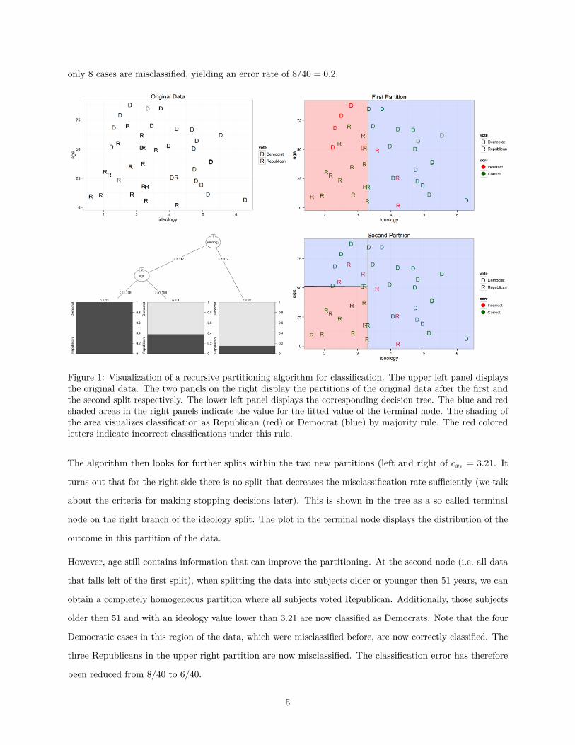
only 8 cases are misclassified, yielding an error rate of 8/40 = 0.2.

Figure 1: Visualization of a recursive partitioning algorithm for classification. The upper left panel displaysthe original data. The two panels on the right display the partitions of the original data after the first andthe second split respectively. The lower left panel displays the corresponding decision tree. The blue and redshaded areas in the right panels indicate the value for the fitted value of the terminal node. The shading ofthe area visualizes classification as Republican (red) or Democrat (blue) by majority rule. The red coloredletters indicate incorrect classifications under this rule.

The algorithm then looks for further splits within the two new partitions (left and right of cx1 = 3.21. It

turns out that for the right side there is no split that decreases the misclassification rate sufficiently (we talk

about the criteria for making stopping decisions later). This is shown in the tree as a so called terminal

node on the right branch of the ideology split. The plot in the terminal node displays the distribution of the

outcome in this partition of the data.

However, age still contains information that can improve the partitioning. At the second node (i.e. all data

that falls left of the first split), when splitting the data into subjects older or younger then 51 years, we can

obtain a completely homogeneous partition where all subjects voted Republican. Additionally, those subjects

older then 51 and with an ideology value lower than 3.21 are now classified as Democrats. Note that the four

Democratic cases in this region of the data, which were misclassified before, are now correctly classified. The

three Republicans in the upper right partition are now misclassified. The classification error has therefore

been reduced from 8/40 to 6/40.

5

We now extend the logic of CART from this very simple example of binary classification with two continuous

predictors to other types of outcome variables. When extending the algorithm to other types of outcome

variables we have to think about loss functions explicitly. In fact, we used a loss function in the illustration

above. We calculated the classification error when just using the modal category of the outcome variable

and argued that further splits of the data are justified because they decrease this error. More formally

let y(m) = (y(m)1 , . . . , y

(m)n(m)) and X(m) = (x(m)

1 , . . . ,x(m)p ) be the data at the current node m, x(m)

s the

explanatory variable that is to be used for a split, with unique values C(m) = {x(m)i }i∈{1,...,n(m)} and c ∈ C(m)

the value considered for a split. Then the data in the daughter nodes resulting from a split in c are y(ml)

and y(mr). Where y(ml) contains all elements of y(m) whose corresponding values of x(m)s ≤ c and y(mr) all

elements where x(m)s > c. The gain (or reduction in error) from a split at node m in predictor xs at value c

is defined as:

∆(y(m)) = L(y(m))−[n(ml)

n(m) L(y(ml)) + n(mr)

n(m) L(y(mr))]

(1)

Where n(ml) and n(mr) are the number of cases that fall to the right and to the left of the split, and L(·) is

the loss function.

In the example above we made the intuitive choice to use the number of cases incorrectly classified when

assigning the mode as the fitted value, divided by the number of cases in the node, as the loss function. In

order to return to the goal stated above, to obtain homogeneous partitions of the data, this proportion can

also be interpreted as the impurity of the data in the node. Therefore it is intuitive to use the amount of

impurity as a measure of loss. This is how the algorithm can be used for outcomes with more than two

unique values (i.e. for nominal or ordinal outcomes with more than two categories, or continuous outcomes).

By choosing a loss function that is appropriate to measure the impurity of a variable at a certain level of

measurement, the algorithm can be extended to those outcomes.

For categorical outcomes, denote the set of unique categories of y(m) as D(m) = {y(m)i }i∈{1,...,n(m)}. In order

to asses the impurity of the node we first calculate the proportion of cases pertaining to each class d ∈ D(m)

and denote it as p(m)(d). Denote further the class that occurs most frequent as y(m). The impurity of the

node in terms of misclassification is then obtained from:

Lmc(y(m)) = 1n(m)

n(m)∑i=1

I(y(m)i 6= y(m)) = 1− p(m)(y(m)) (2)

Where I(·) is the indicator function that is equal to one when its input is true. This formalizes the intuition

6

used above: the impurity of the node is the proportion of cases that would be misclassified under majority

rule.2

A different loss function is required to measure the impurity of the node, when the outcome is continuous.

Usually the mean squared error (MSE) is used:3

Lmse(y(m)) =n(m)∑i=1

(y(m)i − y(m))2 (3)

Where the predicted value y(m) is usually the mean of the observations in y(m). The extension to ordered

discrete predictors is straightforward. Since the observed values of a continuous random variable are discrete,

the partitioning algorithm described above works in the same way for ordered discrete random variables.

Unordered categorical variables are handled differently. If a split in category c of an unordered discrete

variable is considered, the categorization in values to the left and to the right of c have no meaning since there

is no ordering to make sense of “left” and “right.” Therefore all possible combinations of the elements of D(m)

that could be chosen for a split are considered. This can lead to problems for variables with many categories.

For an ordered discrete variable the number of splits that the algorithm has to consider is |D(m)|− 2, however,

for an unordered variable it is 2|D(m)|−1 − 1. This number gets large very quickly. For example the inclusion

of a country indicator as an explanatory variable might be computationally prohibitive if there are more

than a handful of countries (e.g. if there are 21 countries in the sample the number of splits that have to be

considered for that variable at each node is more than a million). Solutions to that problem are to include a

binary variable for each category or to randomly draw a subset of categories at each node (see Louppe 2014,

for details on the latter method).

After a loss function is chosen, the algorithm proceeds as described in our example. At each node m, ∆(y(m))

is calculated for all variables and all possible splits in the variables. The variable-split combination that

produces the highest ∆ is selected and the process is repeated for the data in the resulting daughter nodes

y(ml) and y(mr) until a stopping criterion is met. The stopping criterion is necessary to avoid trees that are

too complex and therefore overfit the data. Theoretically a tree could be grown until there is no impurity in

any terminal nodes. This tree would do perfectly on the data to which it was fit but would perform very

poorly on new data, because any noise in the data to which the CART was fit that was not a part of the2The other two loss functions that are most often used are the Gini loss Lgini(y(m)) =

∑d∈D(m) p(m)(d)[1 − p(m)(d)], and

the entropy of the node Lent(y(m)) = −∑

d∈D(m) p(m)(d) log[p(m)(d)]. Extensive theoretical (e.g. Raileanu and Stoffel 2004)and empirical (e.g. Mingers 1989) work in the machine learning literature concluded that the choice between those measuresdoes not have a significant impact on the results of the algorithm.

3If yet another loss function is employed, the Random Forest algorithm can also be applied to censored data. See Ishwaran etal. (2008) and Hothorn et al. (2006) for details.

7

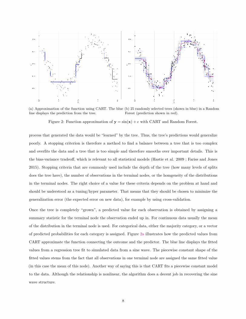
(a) Approximation of the function using CART. The blueline displays the prediction from the tree.

(b) 25 randomly selected trees (shown in blue) in a RandomForest (prediction shown in red).

Figure 2: Function approximation of y = sin(x) + ε with CART and Random Forest.

process that generated the data would be “learned” by the tree. Thus, the tree’s predictions would generalize

poorly. A stopping criterion is therefore a method to find a balance between a tree that is too complex

and overfits the data and a tree that is too simple and therefore smooths over important details. This is

the bias-variance tradeoff, which is relevant to all statistical models (Hastie et al. 2009 ; Fariss and Jones

2015). Stopping criteria that are commonly used include the depth of the tree (how many levels of splits

does the tree have), the number of observations in the terminal nodes, or the homgeneity of the distributions

in the terminal nodes. The right choice of a value for these criteria depends on the problem at hand and

should be understood as a tuning/hyper parameter. That means that they should be chosen to minimize the

generalization error (the expected error on new data), for example by using cross-validation.

Once the tree is completely “grown”, a predicted value for each observation is obtained by assigning a

summary statistic for the terminal node the observation ended up in. For continuous data usually the mean

of the distribution in the terminal node is used. For categorical data, either the majority category, or a vector

of predicted probabilities for each category is assigned. Figure 2a illustrates how the predicted values from

CART approximate the function connecting the outcome and the predictor. The blue line displays the fitted

values from a regression tree fit to simulated data from a sine wave. The piecewise constant shape of the

fitted values stems from the fact that all observations in one terminal node are assigned the same fitted value

(in this case the mean of this node). Another way of saying this is that CART fits a piecewise constant model

to the data. Although the relationship is nonlinear, the algorithm does a decent job in recovering the sine

wave structure.

8

Predicted values for new data can be obtained in a straightforward manner. Starting at the first node of the

tree, a new observation i is “dropped down the tree”, according to its values of the predictors (xi1, ..., xip).

That is, at each node the observation is either dropped to the right or the left daughter node depending

on its value on the explanatory variable that was used to make a split at that node. This way, each new

observation ends up in one terminal node. Then the predicted value of this terminal node is assigned as the

prediction of the tree for observation i.

As previously mentioned CART has one main problem: fitted values have high variance, i.e., there is a risk of

overfitting. Fitted values can be unstable, producing different classifications when changes to the data used to

fit the model are made. There are several related reasons why this occurs. The first is that CART is locally

optimal (greedy). At each step CART selects the split that maximizes the reduction in the loss function

(see Equation 1). It could be the case that if a less than optimal split were taken at one step, a bigger gain

could be had at subsequent steps, that is, local loss minimization may not lead to the global minimum that

could (theoretically) be achieved. Globally optimal solutions to this problem are generally computationally

intractable.4 Given this locally optimal optimization, order effects result, i.e., the order in which the variables

are split can result in different resulting tree structures, and thus, different predictions. Again, this is another

way of saying that CART is a high variance estimator of the function connecting the explanatory variables

to the outcome; the structure discovered varies substantially under stochastic perturbations of the data. In

addition to this issue, it Random Forests, which we discuss in the next section, have generally lower variance.

Combining the Trees to a Forest

Breiman (1996) proposed bootstrap aggregating – “bagging” – to decrease the variance of fitted values from

CART. This innovation is used to reduce the risk of overfitting. The core idea of bagging is to decrease

the variance of the predictions of one model, by fitting several models and averaging over their predictions

to obtain one regularized prediction. In order to obtain a variety of models that are not overfit to the

available data, each component model is fit only to a bootstrap sample of the data. A bootstrap sample is

a sample of the same size as the original data set, but drawn with replacement. Therefore, each of those

samples excludes some portion of the data, which is referred to as “out-of-bag” (OOB) data. In order to

build a Random Forest, a CART is fit to each of the bootstrap samples. Then, predictions from each tree

are obtaind for the OOB data by dropping it down the tree that was grown without that data. Thus each

observation will have a prediction made by each tree where it was not in the bootstrap sample drawn for that

tree. The predicted values for each observation are combined to produce an ensemble estimate which has a4Though see Grubinger, Zeileis, and Pfeiffer for an example of a stochastic search algorithm for this problem.

9

lower variance than would a prediction made by a single CART grown on the original data. For continuous

outcomes the predictions made by each tree are averaged. For discrete outcomes the majority class is used

(or the predicted probabilities are averaged). Relying on the OOB data for predictions also eliminates the

risk of overfitting since the each tree’s prediction is made with data not used for fitting (though see a later

section on limitations and future directions).

Breiman (2001a) extended the logic of bagging to predictors. This means that, instead of choosing the split

from among all the explanatory variables at each node in each tree, only a random subset of the explanatory

variables are used. This might seem counterintuitive at first, but it has the effect of diversifying the splits

across trees. If there are some very important variables they might overshadow the effect of weaker predictors

because the algorithm searches for the split that results in the largest reduction in the loss function. If at each

split only a subset of predictors are available to be chosen, weaker predictors get a chance to be selected more

often, reducing the risk of overlooking such variables. Additionally this allows a very large set of predictors to

be analyzed. If the number of predictors is very large and there are enough trees in the ensemble, all relevant

variables will be chosen for splits eventually, and their impact can be analyzed as well (see the later sections

on how to extract substantive information from the Random Forest). With individual trees in the ensemble

grown on independent sets of data and with different subsets of predictors available, trees give predictions

that are more diverse than if they were grown with the same data or with the same set of predictors. Thus

this reduces the variance of the predictions. This is easy to see by considering the variance of the arithmetic

mean of a stochastic data source drawn from some distribution. The variance of such an estimator decreases

at a rate of σ2/n, where σ2 is the true variance of the data, and n is the sample size. Clearly as n increases

the variability of the estimator decreases as well. Likewise a Random Forest’s predictions for y are an average

(or a modal category for classification). If this estimate is made by combining independent data (each tree’s

predictions) then the variance of the ensemble estimator is decreased more than if the tree’s predictions are

dependent. Roughly, this is because each datum in the average contains less information, and so the effective

sample size is much smaller than n.

A particular observation can fall in the terminal nodes of many trees in the forest, each of which, potentially,

can give a different prediction. Again, the OOB data, that is, data that was not drawn in the bootstrap

sample used to fit a particular tree, is used to make each tree’s prediction. For continuous outcomes, the

prediction of the forest is then the average of the predictions of each tree:

f(X) = 1T

T∑t=1

f (t)(Xi∈B(t)) (4)

10

where T is the total number of trees in the forest, and f (t)(·) is the t’th tree, B(t) is the out-of-bag data

for the t’th tree, that is, observations in X(t) and not in B(t), the bootstrap sample for the t’th tree. For

discrete outcomes, the prediction is the majority prediction from all trees that have been grown without the

respective observation or the average of the predicted probabilities. Figure 2b displays a Random Forest

approximation to a sine wave, which relates a single predictor to a continuous output. The blue lines are

predictions individual predictions from a random selection of 25 trees from the Random Forest, and the

smoother red line represents the prediction from the entire forest. It can be observed that the approximation

is much smoother compared to the approximation by any single tree (Figure 2a).

The number of candidate predictors available at each node and the number of trees in the forest are again

tuning parameters and the optimal choice depends on the data and task at hand. Therefore, they should be

chosen to minimize expected generalization error for example by using resampling methods such as cross

validation. Random Forests compare favorably with other popular nonparametric methods in prediction

tasks and can be interpreted substantively as well as we will show in the following sections (see e.g., Breiman

2001a; Breiman 2001b; Cutler et al. 2007; Murphy 2012; Hastie et al. 2009).

Exploratory Data Analysis and Substantive Interpretation

As could be seen in the section on CART, a single tree is relatively easy to interpret. It can be visualized as

in Figure 1 and directly interpreted. But how is it possible to interpret a thousand trees, every single one

only fit to a sample of the data, and using a random sample of explanatory variables at each split? Because

the Random Forest is an ensemble, it would be fruitless to try to extract substantive insight from its pieces.

However, several methods have been developed to extract more information than just predictions from it. In

this section we explain these methods and how to interpret them substantively using visualizations from our

R software package.

In order to illustrate the practical application of Random Forests for EDA, we use two data examples from

recently published political science studies. The first is a turnout study on released prisoners (Gerber et al.

2014). This dataset contains information on the experimental treatments as well as four additional covariates,

on over 5000 former inmates from Connecticut prisons that were released and whose voting rights have been

restored. As the treatment Gerber et al. (2014) sent letters with two different treatments (the control group

was not contacted), encouraging them to register and vote. Turnout and registration rates were recorded.

The authors found that their treatment had positive effects on registration and turnout. Since registration

and turnout rates are very low in this population and in order to avoid a very imbalanced outcome, we

11

use the subsample of registered prisoners and use their turnout as the outcome. We chose this data set to

show that Random Forests are useful not only in classical data mining applications with large numbers of

predictors, but also for analysis in more standard political science applications.

Additionally we consider data from a recent study of cross-national patterns of state repression (Hill Jr. and

Jones 2014). Quantitative analysis of cross-national patterns of state repression relies on annual country

reports from Amnesty International and the United States Department of State, which are used to code

ordinal measures of state repression such as the Cingranelli and Richards Physical Integrity Index and the

Political Terror Scale (Cingranelli and Richards 2010; Wood and Gibney 2010). We use the measure from

Fariss (2014) which is based on a dynamic measurement model, which aggregates information from multiple

sources on state repression in each country-year into a continuous measure. Hill Jr. and Jones (2014) use data

from 1981 to 1999 in their original study, however, the Random Forest algorithm assumes independent data

(see the later section on limitations). Since the measures of state repression are highly correlated over time

within countries, for the purpose of this demonstration we use data just from 1999. The data set contains

data on 190 countries. We use a set of explanatory variables that differs slightly from that of Hill Jr. and

Jones (2014), containing some predictors that may be relevant but were omitted before, and some predictors,

such as the participation competitiveness component of Polity IV, and binary indicators for civil war, which

have conceptual overlap with respect for physical integrity rights and should be omitted on those grounds

(Hill Jr. and Jones 2014; Hill Jr 2014). This data is well suited for exploratory data analysis using Random

Forests because we have no expectation that the relationship between any particular predictor (that is not

binary) will have a linear (or even smooth) relationship with our measure of respect for physical integrity

rights, nor do we have expectations about the number or size of any interactions that may be present in the

data. However, we would like to discover such relationships if they exist. Additionally, by studying the latent

similarity of countries in the predictor space, we hope to notice features of countries close in this space which

we do not have data on, and might be fruitful areas of future research.

Variable Importance

Often the goal of EDA is to identify variables that might be theoretically interesting, in order to generate

hypotheses for later confirmatory analyses. Especially with the rise of big data, in many cases information

on an abundance of variables that could not be considered before is available. In such instances a method

to quickly asses the importance of a large set of explanatory variables is very useful. With permutation

importance Random Forests provide a very useful tool for this purpose. It relies on the predictive importance

of variables, which in many cases can give a more relevant measure of substantive importance than, for

12

example, statistical significance tests (Gill 1999; Shmueli 2010).

The marginal permutation importance shows the mean decrease in prediction error that results from randomly

permuting an explanatory variable. If a particular column of X, say xj , is unrelated to y, then randomly

permuting xj within X should not meaningfully decrease the model’s ability to predict y5. However, if xj is

strongly related to y, then permuting its values will produce a systematic decrease in the model’s ability

to predict y, and the stronger the relationship between xj and y, the larger this decrease. Averaging the

amount of change in the fitted values from permuting xj across all the trees in the forest gives the marginal

permutation importance of a predictor6. Formally the importance of explanatory variable xj in tree t ∈ T is:

VI(t)(xj) = L(y(t), y(t))− L(y(t), y(t)π ) (5)

Where t indexes trees, xj is a particular predictor, y(t) are the fitted values for tree t, and y(t)π are the fitted

values for y(t) after permuting xj . L(·) is the loss function. For categorical outcomes the loss function usually

used is the misclassification rate (Equation 2), entropy or gini impurity (see Footnote 3). For regression the

mean squared error (Equation 3) is used. In words, the importance in a single tree is simply the difference

between the predictive accuracy (measured on the out-of-bag data) before and after permuting xj . The

importance of variable xj in tree t is averaged across all trees to obtain the permutation importance for the

whole forest (Equation 6) (Breiman 2001a; Strobl et al. 2008):

VI(xj) = 1T

T∑t=1

VI(t)(xj) (6)

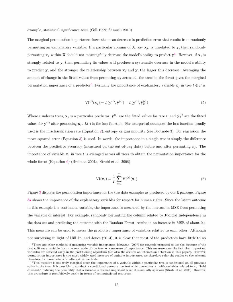
Figure 3 displays the permutation importance for the two data examples as produced by our R package. Figure

3a shows the importance of the explanatory variables for respect for human rights. Since the latent outcome

in this example is a continuous variable, the importance is measured by the increase in MSE from permuting

the variable of interest. For example, randomly permuting the column related to Judicial Independence in

the data set and predicting the outcome with the Random Forest, results in an increase in MSE of about 0.4.

This measure can be used to assess the predictive importance of variables relative to each other. Although

not surprising in light of Hill Jr. and Jones (2014), it is clear that most of the predictors have little to no5There are other methods of measuring variable importance. Ishwaran (2007) for example proposed to use the distance of the

first split on a variable from the root node of the tree as a measure of importance. This measure uses the fact that importantvariables are selected early in the partitioning algorithm (see also the section on interaction detection in this paper). However,permutation importance is the most widely used measure of variable importance, we therefore refer the reader to the relevantliterature for more details on alternative methods.

6This measure is not truly marginal since the importance of a variable within a particular tree is conditional on all previoussplits in the tree. It is possible to conduct a conditional permutation test which permutes xj with variables related to xj “heldconstant,” reducing the possibility that a variable is deemed important when it is actually spurious (Strobl et al. 2008). However,this procedure is prohibitively costly in terms of computational resources.

13

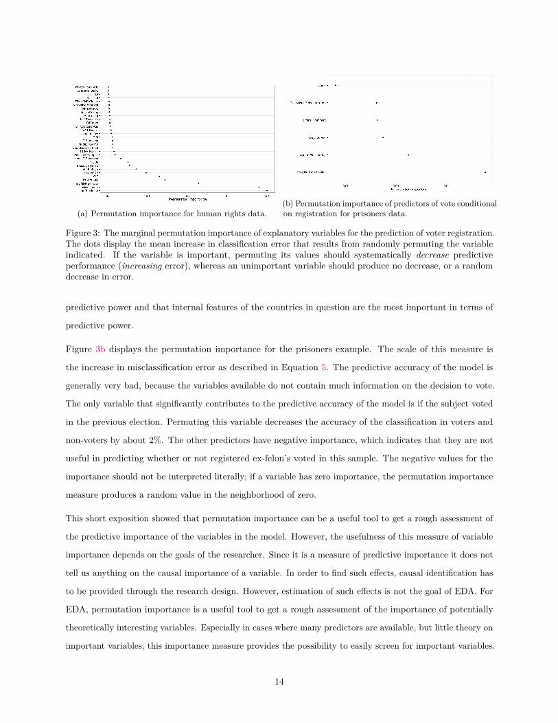
(a) Permutation importance for human rights data.(b) Permutation importance of predictors of vote conditionalon registration for prisoners data.

Figure 3: The marginal permutation importance of explanatory variables for the prediction of voter registration.The dots display the mean increase in classification error that results from randomly permuting the variableindicated. If the variable is important, permuting its values should systematically decrease predictiveperformance (increasing error), whereas an unimportant variable should produce no decrease, or a randomdecrease in error.

predictive power and that internal features of the countries in question are the most important in terms of

predictive power.

Figure 3b displays the permutation importance for the prisoners example. The scale of this measure is

the increase in misclassification error as described in Equation 5. The predictive accuracy of the model is

generally very bad, because the variables available do not contain much information on the decision to vote.

The only variable that significantly contributes to the predictive accuracy of the model is if the subject voted

in the previous election. Permuting this variable decreases the accuracy of the classification in voters and

non-voters by about 2%. The other predictors have negative importance, which indicates that they are not

useful in predicting whether or not registered ex-felon’s voted in this sample. The negative values for the

importance should not be interpreted literally; if a variable has zero importance, the permutation importance

measure produces a random value in the neighborhood of zero.

This short exposition showed that permutation importance can be a useful tool to get a rough assessment of

the predictive importance of the variables in the model. However, the usefulness of this measure of variable

importance depends on the goals of the researcher. Since it is a measure of predictive importance it does not

tell us anything on the causal importance of a variable. In order to find such effects, causal identification has

to be provided through the research design. However, estimation of such effects is not the goal of EDA. For

EDA, permutation importance is a useful tool to get a rough assessment of the importance of potentially

theoretically interesting variables. Especially in cases where many predictors are available, but little theory on

important variables, this importance measure provides the possibility to easily screen for important variables.

14

This is an attractive alternative to null hypothesis significance testing, which is often used heuristically for

this purpose (Hill Jr. and Jones 2014; Ward, Greenhill, and Bakke 2010; Gill 1999). NHST can be thought of

as giving a measure of surprise under the assumption of the null (e.g. that a regression coefficient is exactly

zero) with a particular type of stochastic variability assumed from the model. However, this can be misleading

when no assumed model is determined by theory, and, consequently, it is likely that the model is misspecified,

perhaps severely. It can also be misleading when this logic does not comport with the analysts’ use of the

word “importance.” In situations where causal identification is difficult or impossible, predictive importance is

a reasonable way to define and measure importance. Additionally, this measure comes from a method which

does not specify a particular generative structure on the data, and hence measures of importance include

direct and indirect associations (i.e., dependence of the outcome on a variable and all interactions that are

detected with that variable). This decreases the chance that a variable could be missed if its direct effects are

masked or dwarfed by its indirect effects.

Interpretation of Relationships

Although the predictive importance of a variable can often be very insightful, most scholars are interested in

how the variable is related to the outcome. Partial dependence is a simple method, again based on predictions

from the forest, to visualize the partial relationship between the outcome and the predictors (Hastie et al.

2009). Partial dependence provides the ability to visualize the relationship between y and one or more

predictors xj as detected by the Random Forest. The basic intuition is to obtain a prediction from the

Random Forest for each unique value of xj (or of each value combination if there are multiple variables of

interest) accounting for the effects of the other variables. Plotting these predictions against the unique values

of xj then displays how y is related to xj according to the model. Since the Random Forest can approximate

almost arbitrary functional relationships between xj and y – as shown in Figure 2b – the model is able

to detect non-linear relationships without the need to pre-specify them. This allows to detect potentially

interesting non-linearities in settings where little a priori theoretical knowledge allows for pre-specification of

specific forms. This is one of the main strengths of Random Forests for exploratory analyses.

The basic way partial dependence works is the following: for each value of the variable of interest, a new

data set is created, where all observations are assigned the same value on the variable of interest. Then this

data set is dropped down the forest, and a prediction for each observation is obtained. By averaging over

these predictions, a prediction for a synthetic data set where the variable of interest is fixed to a particular

value, and all other predictors are left unchanged is obtained. This is similar in spirit to integrating over the

variables that are not in the subset of interest, however, since we have no explicit probability model, we use

15

this empirical procedure. Repeating this for all values of the variable of interst gives the relationship between

said variable and the outcome over its range. Let xj be the predictor of interest, X−j be the other predictors,

y be the outcome, and f(X) the fitted forest. Then, in more detail, the partial dependence algorithm works

as follows:

1. For xj sort the unique values V = {xj}i∈{1,...,n} resulting in V∗, where |V∗| = K. Create K new

matrices X(k) = (xj = V∗k ,X−j), ∀ k = (1, . . . ,K).

2. Drop each of the K new datasets, X(k) down the fitted forest resulting in a predicted value for each

observation in all k datasets: y(k) = f(X(k)), ∀ k = (1, . . . ,K).

3. Average the predictions in each of the K datasets, y∗k = 1n

∑Ni=1 y

(k)i , ∀ k = (1, . . . ,K).

4. Visualize the relationship by plotting V∗ against y∗.

The average predictions obtained from this method are more than just marginal relationships between the

outcome and the predictor. Since each of the predictions are made using all the information in all the other

predictors of an observation, the prediction obtained from the partial dependence algorithm also contains

this information. This means that the relationship displayed in a partial dependence plot contains all the

relation between xj and y including the averaged effects of all interactions of xj with all the other predictors

X−j , which is why this method gives the partial dependence rather than the marginal dependence.

Our software provides a method to compute k-way partial dependence (i.e., interactions of arbitrary dimension

or many two-way partial dependencies) for continuous, binary, categorical, censored, and multivariate outcome

variables. Note again that partial dependence differs from obtaining predictions for y with (xj ,x−j) fixed

(i.e., setting the values of x−j as well as those in xj). Instead partial dependence gives predictions for y

conditional on xj given the average effects of x−j (p. 369-371 Hastie et al. 2009).

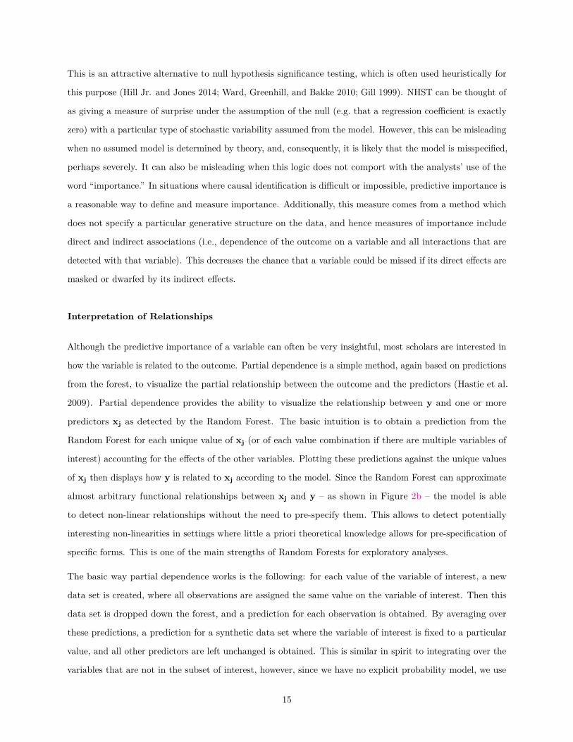
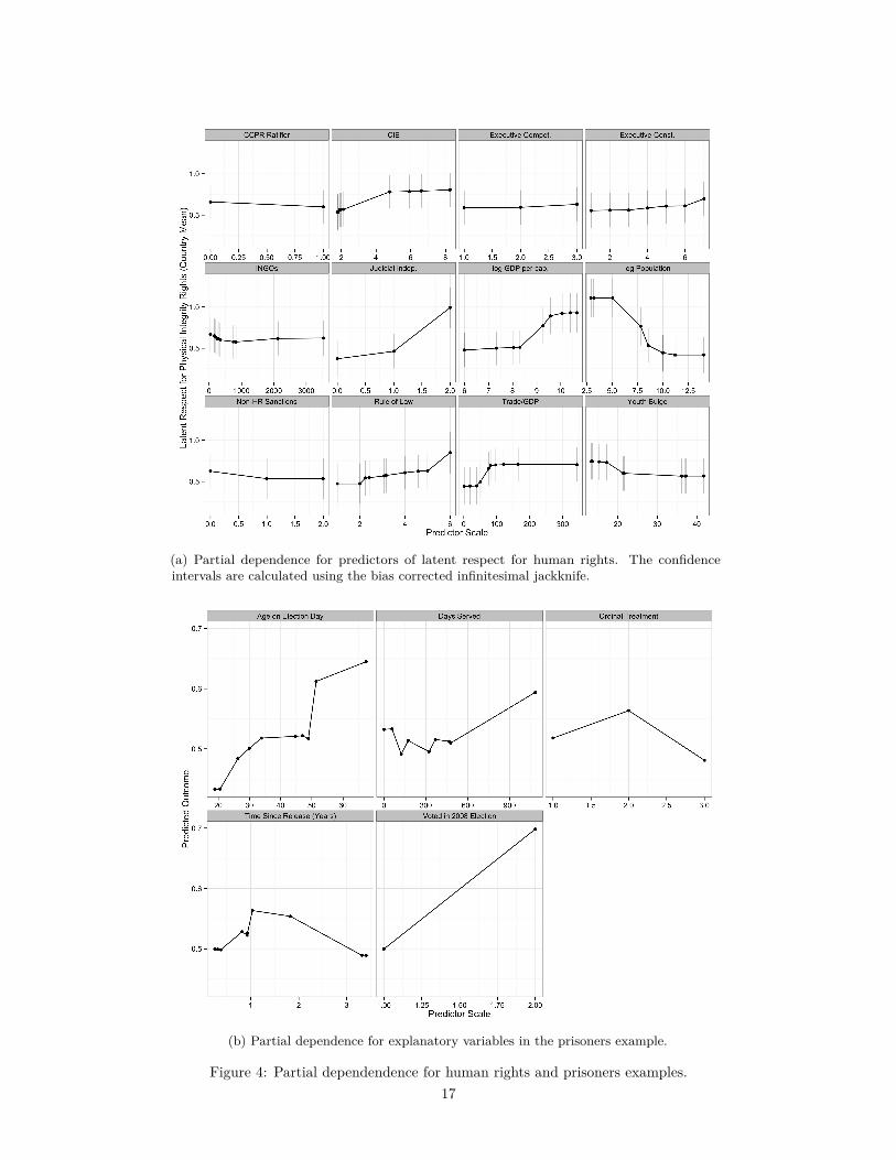
Figure 4 diplays the partial dependence for our example data sets. Figure 4a displays the relationships of

selected predictors with the latent outcome variable. Figure 4b shows the results for the prisoners example.

Note that the partial dependence plots in 4a additionally contain error bars for the predictions, whereas there

are no such bars in the plots for the prisoners example. Estimating sampling uncertainty for predictions from

ensemble algorithms such as random forests is a relatively new area of research (Sexton and Laake 2009;

Wager, Hastie, and Efron 2014; Mentch and Hooker 2014). Wager, Hastie, and Efron (2014) developed a

method – the bias-corrected infinitesimal jackknife (BIJ) to produce variance estimates for predictions from

Random Forests. However, this method works only for continuous outcomes and not for classification. We

implemented the BIJ in our R package to produce uncertainty intervals for partial dependence plots. Since

16

(a) Partial dependence for predictors of latent respect for human rights. The confidenceintervals are calculated using the bias corrected infinitesimal jackknife.

(b) Partial dependence for explanatory variables in the prisoners example.

Figure 4: Partial dependendence for human rights and prisoners examples.17

this is a topic of ongoing research, and there are other proposed approaches, we expect to extend our software

to these approaches (see e.g. Hooker 2004).

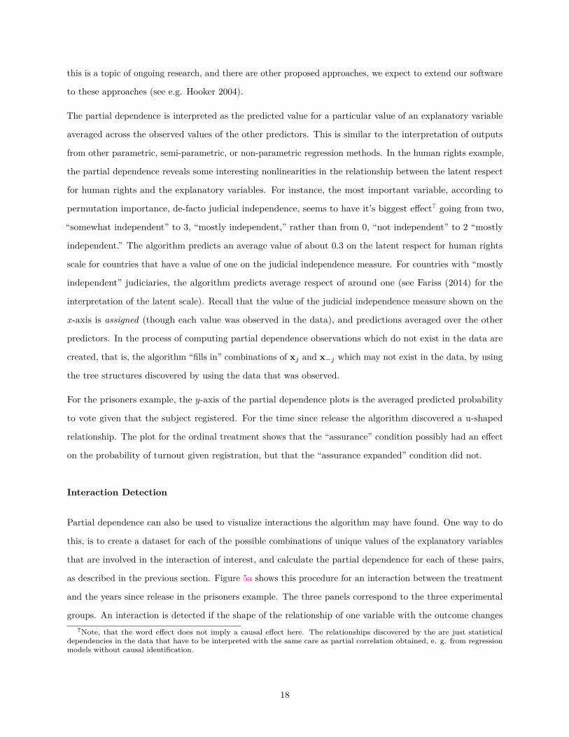
The partial dependence is interpreted as the predicted value for a particular value of an explanatory variable

averaged across the observed values of the other predictors. This is similar to the interpretation of outputs

from other parametric, semi-parametric, or non-parametric regression methods. In the human rights example,

the partial dependence reveals some interesting nonlinearities in the relationship between the latent respect

for human rights and the explanatory variables. For instance, the most important variable, according to

permutation importance, de-facto judicial independence, seems to have it’s biggest effect7 going from two,

“somewhat independent” to 3, “mostly independent,” rather than from 0, “not independent” to 2 “mostly

independent.” The algorithm predicts an average value of about 0.3 on the latent respect for human rights

scale for countries that have a value of one on the judicial independence measure. For countries with “mostly

independent” judiciaries, the algorithm predicts average respect of around one (see Fariss (2014) for the

interpretation of the latent scale). Recall that the value of the judicial independence measure shown on the

x-axis is assigned (though each value was observed in the data), and predictions averaged over the other

predictors. In the process of computing partial dependence observations which do not exist in the data are

created, that is, the algorithm “fills in” combinations of xj and x−j which may not exist in the data, by using

the tree structures discovered by using the data that was observed.

For the prisoners example, the y-axis of the partial dependence plots is the averaged predicted probability

to vote given that the subject registered. For the time since release the algorithm discovered a u-shaped

relationship. The plot for the ordinal treatment shows that the “assurance” condition possibly had an effect

on the probability of turnout given registration, but that the “assurance expanded” condition did not.

Interaction Detection

Partial dependence can also be used to visualize interactions the algorithm may have found. One way to do

this, is to create a dataset for each of the possible combinations of unique values of the explanatory variables

that are involved in the interaction of interest, and calculate the partial dependence for each of these pairs,

as described in the previous section. Figure 5a shows this procedure for an interaction between the treatment

and the years since release in the prisoners example. The three panels correspond to the three experimental

groups. An interaction is detected if the shape of the relationship of one variable with the outcome changes7Note, that the word effect does not imply a causal effect here. The relationships discovered by the are just statistical

dependencies in the data that have to be interpreted with the same care as partial correlation obtained, e. g. from regressionmodels without causal identification.

18

across levels of the other variable. In Figure 5a there is a shift in the probability to vote, but the shape of

the relationship changes only slightly, indicating that the algorithm has not detected a strong interaction.

In this case we are examining a possible interaction between a continuous variable and a discrete variable

with only three values, however, if the variables involved in a potential interaction are both continuous or

categorical with many levels, two problems occur. First, it would be computationally prohibitive to calculate

the partial dependence for all combinations of values of the two variables. For instance, if analyzing the

interaction between two variables with 50 and 100 unique values, 50× 100 = 5000 data sets would have to

be created and processed by the partial dependence algorithm. Depending on the size of the data set and

the computational resources available to the researcher, this might be prohibitive. Second, the visualization

becomes more difficult, because the there are two many value combinations making a display as in Figure 5a

infeasible.

We solve the first problem by taking a random sample of unique values that are used in the algorithm8

(but always including the minimum and maximum of the variables involved to obtain a picture of the whole

range of both variables). The reduction of the number of values that is achieved with this strategy also

makes visualization easier. The number of unique values can be further decreased by assigning the values of

continuous variables to a set of bins, and assigning the combinations of these bins in the partial dependence

algorithm. Another option for visualization, if reduction of unique values is not desirable, is to use three

dimensional plots, as displayed in Figure 5b. In this simulated example, the height of the plot represents the

predicted value at each value combination, whereas the two horizontal axes represent the two variables of

interest. The interaction between the variables is clearly visible in this example, because the shape of the

marginal relationships of each variable with the outcome changes conditional on the value of the interacting

variable.

Theoretically, higher order interactions could be detected in this way as well. If, for instance, a potential

three-way interaction is considered, all combinations of the unique values of the three variable can be obtained

and partial dependence can be calculated. In addition to the computational demand of such a procedure, the

partial dependence itself is difficult to interpret and is almost exclusively useful when visualized. In practice,

it is therefore hard to consider interactions of a higher order for substantive interpretation9. In order to

screen the set of explanatory variables for interactions, the partial dependence of all variable pairs has to be

calculated and visually inspected. Depending on the number of predictor variables this procedure might be8It is also possible to use an evenly spaced grid, however, this may result in extrapolation. Both of these options are

implemented in our R package.9Although it is difficult to interpret these higher order interactions, they are still detected by the Random Forest algorithm

and built into the model after it is fitted. The information from such higher order interactions is therefore still contained inpredictions obtained from the forest.

19

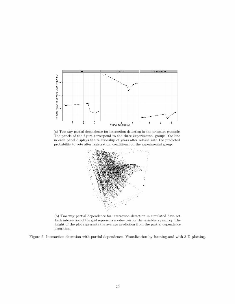
(a) Two way partial dependence for interaction detection in the prisoners example.The panels of the figure correspond to the three experimental groups, the linein each panel displays the relationship of years after release with the predictedprobability to vote after registration, conditional on the experimental group.

(b) Two way partial dependence for interaction detection in simulated data set.Each intersection of the grid represents a value pair for the variables x1 and x2. Theheight of the plot represents the average prediction from the partial dependencealgorithm.

Figure 5: Interaction detection with partial dependence. Visualization by faceting and with 3-D plotting.

20

computationally and time intensive. However, we our software optionally parallelizes the computation of

partial dependence making it possible to distribute the task across multiple computers.

Another method of detecting interactions from Random Forests does not rely so heavily on visualization.

Instead, it uses maximal v-subtrees and minimal depth (Ishwaran 2007; Ishwaran et al. 2010; Ishwaran et al.

2011). The basic idea behind this method for interaction detection is the fact that in CART variables that

are used for splits on a higher level (i.e. closer to the root node) have higher importance for prediction10. The

measure of interactive importance of two variables, say v and w is the depth of the first split on w within a

tree that is defined by the first split on v. More formally, Ishwaran et al. (2010) introduce the concept of a

maximal v-subtree. A maximal subtree for a variable v is the largest subtree of a tree that has as its root

node a split on v, and no split on v in the parent nodes of this root node. The minimal depth for variable

v is the distance between the highest maximal subtree for variable v and the root node of the whole tree.

The minimal depth is therefore a measure of the predictive importance of v. Interactions between pairs of

variables v and w can be detected, by calculating the minimal depth of w in the maximal subtree of v and

averaging this measure over all trees in the forest. This calculation gives a matrix of size p× p (recall that p is

the number of variables), that has on the diagonal the importance (according to the minimal depth criterion)

of each variable, and on the off-diagonal elements the importance of the pairs of variables. This matrix can

be easily scanned for rows that have a high importance on the diagonal entry and high importance on the off

diagonals indicating interactions with these variables11.

Again, this method can only detect interactions between pairs of variables. There are, to our knowledge, no

direct ways to detect and interpret interactions of higher orders. However, the interactions are still contained

in the fitted forest. This means, the information about these interactions are contained in all predictions and,

when they exist, discovered by multivariate partial dependence.

Similarity and Clustering

Random Forests can furthermore be used to to understand the similarity between observations in the predictor

space. Since observations that have similar x values ‘travel’ the same way on splits more often than values

with dissimilar values, the co-occurence in terminal nodes is a suitable measure of similarity. Using this logic

a so called proximity matrix is calculated. It is a n by n matrix where each entry gives the proportion of10This fact can also be used to create a measure of variable importance; an alternative to the permutation importance measure

described above.11We are currently working on the implementation of a visualization tool for this method across packages. Currently maximal

subtrees and minimal depth can only be obtained from the randomForestSRC package. Another method to detect interactionrelies on joint and marginal variable importance. Calculating the predictive importance of a pair of variables and subtractingthe marginal importance of the single variables gives a measure of interactive importance. See Ishwaran (2007) for more detailson this method.

21

times that observation i is in the same terminal node as observation j across all the terminal nodes in the

different trees of the forest.

In order to interpret this large proximity matrix, factorization methods such as principle components analysis

(PCA) can be used to visualize the similarity of the observations. PCA can be effectively visualized using

a biplot (Gabriel 1971). Our software provides a unified interface for extracting and visualizing proximity

matrices from the different Random Forest packages in R. We also make it easy to layer additional variables

through coloring or shape on top of a biplot. Such biplots for our example data are displayd in Figures 6 and

7.

In Figure 6a observations are coloured by their treatment condition, and in Figure 6b, by whether or not

they voted (the outcome of interest). The point shape shows whether or not the individual voted in 2008,

and the size of the point gives the individual’s age on election day. Clearly the first component (the x-axis) is

whether or not the individual voted in 2008, and the second component is treatment status. Age appears to

be less directly relevant. Decompositions of the proximity matrix can provide additional information about

the importance of the explanatory variables when they account for a relatively large portion of the variance

of the proximity matrix. In this case whether or not an individual voted in 2008 and their treatment status

were the dominant axes, however it appears that treatment status is less important than previous voting.

When individual data points are labelled these visualizations of the proximity matrix can provide additional

insight into similarity between units conditional on the relationship between the explanatory variables and the

outcome as discovered by the Random Forest. Figure 7 shows a biplot of the first two principal components

applied to a Random Forest fit to the human rights data. De-facto judicial independence from CIRI is used

to color the country names (Cingranelli and Richards 2010). Although it does not appear that judicial

independence is first principal component shown on the x-axis, there appears to be some separation on the

x-axis on this measure. There appears to be some spatial clustering (for example, many Nordic countries

cluster tightly in the lower left-hand corner), as well as clustering according to size/population.

22

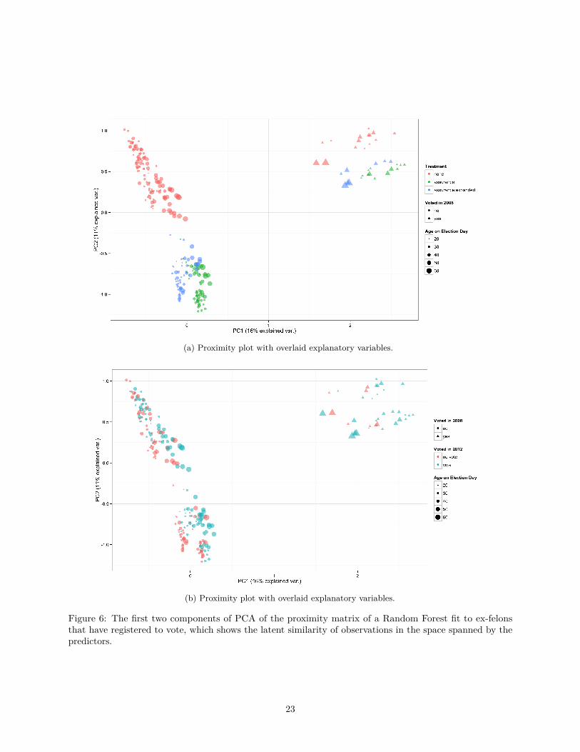
(a) Proximity plot with overlaid explanatory variables.

(b) Proximity plot with overlaid explanatory variables.

Figure 6: The first two components of PCA of the proximity matrix of a Random Forest fit to ex-felonsthat have registered to vote, which shows the latent similarity of observations in the space spanned by thepredictors.

23

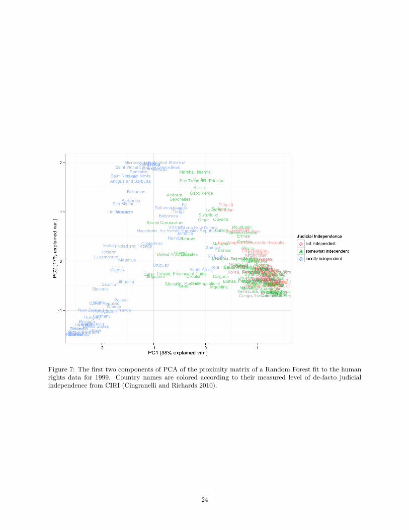
Figure 7: The first two components of PCA of the proximity matrix of a Random Forest fit to the humanrights data for 1999. Country names are colored according to their measured level of de-facto judicialindependence from CIRI (Cingranelli and Richards 2010).

24

Limitations and Future Directions

Random Forests are not without issue however. The CART which they are composed of often rely on biased

splitting criteria: some types of variables, specifically variables with many unique values, are artificially

preferred to variables with fewer categories (Hothorn, Hornik, and Zeileis 2006; Strobl et al. 2007). These

biases can also affect the measures of variable importance. Recent developments have resulted in unbiased

recursive partitioning algorithms that separate the variable selection and split selection parts of the CART

algorithm, and utilize subsampling rather than bootstrapping (Hothorn, Hornik, and Zeileis 2006). The

analyses in this paper are done using this unbiased algorithm.

Furthermore, as with many other methods, Random Forests utilize methods which assume that the observations

in the sample are independent. Theoretical results regarding the consistency of Random Forests for estimation

of moments (e.g., the mean) of the conditional distribution of the outcome rely on this assumption, and

there is evidence to suggest that violation of this assumption results in degradation of predictive performance

(Breiman 2001a; Wager and Walther 2015). However, there are several ways of dealing with this issue.

First, features of the dependence structure can often be incorporated as explanatory variables. Then, at

each node in each tree in the forest, these variables have a chance of being included in the set of variables

that may be split on. This means that if an explanatory variable has a relationship with the outcome that

changes across different units, time, etc., this can be detected if the structure is included in this way. However,

when such a description of the data structure results in unordered categorical variables with many unique

categories, this is computationally intensive and not always possible. As mentioned in the section on CART,

inclusion of a country indicator might already be prohibitive if there are more than 20 countries.

Second, there exist a variety of nonparametric resampling methods which can be used in place of independent

bootstrapping. The generalized moving block bootstrap, transformation based bootstraps, or model-based

(filtering) bootstrapping are examples of nonparametric bootstraps for dependent data, but the appropriateness

of any particular method is context specific (Lahiri 2003). Using an appropriate resampling method that

only exchanges statistically independent observations has the effect of decreasing the correlation between

trees in the forest, making them more diverse, and consequentially reducing variance (Breiman 2001a). A

Random Forest with trees grown on data that are bootstrapped in a way that does not take into account

the dependence structure will produce more correlated predictions, and higher variance predictions, which is

another way of saying that there may be overfitting. Furthermore, if inappropriate resampling methods are

used for hyperparameter optimization (e.g, the maximal depth of trees or the number of variables considered

at each node), this will result in poor estimates of generalization error (the OOB error) and consequently will

25

induce too much or too little complexity depending on the dependence in the data.

Lastly, a random effects approach could be used: the outcome of interest is treated as a function of an

unknown regression function which is estimated using Random Forests. The error is decomposed into variance

attributable to aspects of the dependence specified in a linear mixed-effects model and idiosyncratic error.

This improves predictions by using variance unexplained by the Random Forest but attributable to features

of the dependence structure (Hajjem, Bellavance, and Larocque 2014; Hajjem, Bellavance, and Larocque

2011). However, this method is currently limited to regression problems.

Conclusion

With the rise of big data and the increasing prominence of computationally intensive methods of analysis,

machine learning algorithms have become more visible to social scientists. Random Forests are a prominent

member of this class of methods. Although Random Forests are commonly used in other disciplines, they have

not been widely used in political science (See, e.g., Cutler et al. 2007; Strobl, Malley, and Tutz 2009; Berk

2006). We suspect that this is in part due to the belief that machine learning methods, which are primarily

designed to achieve good predictive performance, are black boxes that are not helpful for substantive research

(Breiman 2001b; Clark and Golder 2015). Additionally, the methods necessary to interpret Random Forests

are not jointly available in a software package that is easy to use for applied researchers. Although most

methods are available somewhere, a lot of effort might be required in many situations in order to extract all

the potential information contained in the Random Forest.

In this paper we gave an introduction to Random Forests and demonstrated several methods that facilitate

their use for substantive research. In situations where relevant theory says little about the functional form

of the relationship of interest, whether or not interactions are present, and when the number of possibly

relevant predictors is large, Random Forests can be a valuable addition to the data analysis tools available to

political scientists. In order to make these tools more accessible for applied researchers, we provide software

that facilitates visualization and substantive interpretation.

Although they might be a powerful new tool to analyze complex data, algorithmic methods are not a

substitute for good research design and careful social scientific reasoning. To avoid such a confusion we

explicitly advertise the use of such methods in an exploratory setting. In such situations, flexible algorithms

can be superior to classical parametric methods which may miss many rich features of the data because their

assumptions may constrain the discovery of such features. Political science can play an important role in

the future directions of machine learning research. Particularly, we see the development of machine learning

26

methods for dependent data as a fruitful area of research for political methodologists, as this data is very

common in our discipline.

27

References

Beck, Nathaniel, and Simon Jackman. 1998. “Beyond Linearity by Default: Generalized Additive Models.”

American Journal of Political Science 42. University of Texas Press: 596–627.

Beck, Nathaniel, Gary King, and Langche Zeng. 2000. “Improving Quantitative Studies of International

Conflict: A Conjecture.” American Political Science Review. JSTOR, 21–35.

Berk, Richard A. 2006. “An Introduction to Ensemble Methods for Data Analysis.” Sociological Methods &

Research 34 (3). Sage Publications: 263–95.

Breiman, Leo. 1996. “Bagging Predictors.” Machine Learning 24 (2). Springer: 123–40.

———. 2001a. “Random Forests.” Machine Learning 45 (1). Springer: 5–32.

———. 2001b. “Statistical Modeling: The Two Cultures (with Comments and a Rejoinder by the Author).”

Statistical Science 16 (3). The Institute of Mathematical Statistics: 199–231. doi:10.1214/ss/1009213726.

Cingranelli, David L., and David L. Richards. 2010. “The Cingranelli-Richards (CIRI) Human Rights

Dataset.” http://www.humanrightsdata.org.

Clark, William Roberts, and Matt Golder. 2015. “Big Data, Causal Inference, and Formal Theory:

Contradictory Trends in Political Science?” PS: Political Science & Politics 48 (01). Cambridge Univ Press:

65–70.

Cutler, D Richard, Thomas C Edwards Jr, Karen H Beard, Adele Cutler, Kyle T Hess, Jacob Gibson, and

Joshua J Lawler. 2007. “Random Forests for Classification in Ecology.” Ecology 88 (11). Eco Soc America:

2783–92.

D’Orazio, Vito, Kenwick Michael R., Matthew A. Lane, Glenn Palmer, and David Reitter. 2015. “There’s

Gotta Be a Better Way: Crowdsourcing the Collection of Observational Data.”

Fariss, Christopher J. 2014. “Respect for Human Rights Has Improved over Time: Modeling the Changing

Standard of Accountability.” American Political Science Review. Cambridge Univ Press, 1–22.

Fariss, Christopher J., and Zachary M. Jones. 2015. “Enhancing Validity in Observational Settings When

Replication Is Not Possible.”

Fernández-Delgado, Manuel, Eva Cernadas, Senén Barro, and Dinani Amorim. 2014. “Do We Need Hundreds

of Classifiers to Solve Real World Classification Problems?” The Journal of Machine Learning Research 15

(1). JMLR. org: 3133–81.

28

Gabriel, Karl Ruben. 1971. “The Biplot Graphic Display of Matrices with Application to Principal Component

Analysis.” Biometrika 58 (3). Biometrika Trust: 453–67.

Gelman, Andrew. 2004. “Exploratory Data Analysis for Complex Models.” Journal of Computational and

Graphical Statistics 13 (4).

Gerber, Alan S, Gregory A Huber, Marc Meredith, Daniel R Biggers, and David J Hendry. 2014. “Can

Incarcerated Felons Be (Re) Integrated into the Political System? Results from a Field Experiment.” American

Journal of Political Science. Wiley Online Library.

Gill, Jeff. 1999. “The Insignificance of Null Hypothesis Significance Testing.” Political Research Quarterly 52

(3). Sage Publications: 647–74.

Grimmer, Justin, and Brandon M Stewart. 2013. “Text as Data: The Promise and Pitfalls of Automatic

Content Analysis Methods for Political Texts.” Political Analysis. SPM-PMSAPSA, mps028.

Grubinger, Thomas, Achim Zeileis, and Karl-Peter Pfeiffer. “Evtree: Evolutionary Learning of Globally

Optimal Classification and Regression Trees in R.”

Hainmueller, Jens, and Chad Hazlett. 2013. “Kernel Regularized Least Squares: Reducing Misspecification

Bias with a Flexible and Interpretable Machine Learning Approach.” Political Analysis. SPM-PMSAPSA,

mpt019.

Hajjem, Ahlem, François Bellavance, and Denis Larocque. 2011. “Mixed Effects Regression Trees for Clustered

Data.” Statistics & Probability Letters 81 (4). Elsevier: 451–59.

———. 2014. “Mixed-Effects Random Forest for Clustered Data.” Journal of Statistical Computation and

Simulation 84 (6). Taylor & Francis: 1313–28.

Hastie, Trevor, Robert Tibshirani, Jerome Friedman, T Hastie, J Friedman, and R Tibshirani. 2009. The

Elements of Statistical Learning. Vol. 2. 1. Springer.

Hill Jr, Daniel W. 2014. “Democracy and the Concept of Personal Integrity Rights in Empirical Research.”

Hill Jr., Daniel W., and Zachary M. Jones. 2014. “An Empirical Evaluation of Explanations for State

Repression.” American Political Science Reivew 108 (3): 661–87.

Hooker, Giles. 2004. “Discovering Additive Structure in Black Box Functions.” In Proceedings of the Tenth

ACM SIGKDD International Conference on Knowledge Discovery and Data Mining, 575–80. ACM.

Hothorn, Torsten, Peter Bühlmann, Sandrine Dudoit, Annette Molinaro, and Mark J Van Der Laan. 2006.

“Survival Ensembles.” Biostatistics 7 (3). Biometrika Trust: 355–73.

29

Hothorn, Torsten, Kurt Hornik, and Achim Zeileis. 2006. “Unbiased Recursive Partitioning: A Conditional

Inference Framework.” Journal of Computational and Graphical Statistics 15 (3).

Imai, Kosuke, and Marc Ratkovic. 2013. “Estimating Treatment Effect Heterogeneity in Randomized Program

Evaluation.” The Annals of Applied Statistics 7 (1). Institute of Mathematical Statistics: 443–70.

Ishwaran, Hemant. 2007. “Variable Importance in Binary Regression Trees and Forests.” Electronic Journal

of Statistics 1. Institute of Mathematical Statistics: 519–37.

Ishwaran, Hemant, Udaya B Kogalur, Eugene H Blackstone, and Michael S Lauer. 2008. “Random Survival

Forests.” The Annals of Applied Statistics 2 (3). JSTOR: 841–60.

Ishwaran, Hemant, Udaya B Kogalur, Xi Chen, and Andy J Minn. 2011. “Random Survival Forests for

High-Dimensional Data.” Statistical Analysis and Data Mining 4 (1). Wiley Online Library: 115–32.

Ishwaran, Hemant, Udaya B Kogalur, Eiran Z Gorodeski, Andy J Minn, and Michael S Lauer. 2010. “High-

Dimensional Variable Selection for Survival Data.” Journal of the American Statistical Association 105 (489).

Taylor & Francis: 205–17.

King, Gary, Jennifer Pan, and Margaret E Roberts. 2013. “How Censorship in China Allows Government

Criticism but Silences Collective Expression.” American Political Science Review 107 (02). Cambridge Univ

Press: 326–43.

———. 2014. “Reverse-Engineering Censorship in China: Randomized Experimentation and Participant

Observation.” Science 345 (6199). American Association for the Advancement of Science: 1251722.

Lahiri, Soumendra Nath. 2003. Resampling Methods for Dependent Data. Springer Science & Business

Media.

Louppe, Gilles. 2014. “Understanding Random Forests: From Theory to Practice.” ArXiv Preprint

ArXiv:1407.7502.

Mentch, Lucas, and Giles Hooker. 2014. “Ensemble Trees and Clts: Statistical Inference for Supervised

Learning.” ArXiv Preprint ArXiv:1404.6473.

Mingers, John. 1989. “An Empirical Comparison of Selection Measures for Decision-Tree Induction.” Machine

Learning 3 (4). Springer: 319–42.

Monroe, Burt L, Jennifer Pan, Margaret E Roberts, Maya Sen, and Betsy Sinclair. 2015. “No! Formal

Theory, Causal Inference, and Big Data Are Not Contradictory Trends in Political Science.” PS: Political

Science & Politics 48 (01). Cambridge Univ Press: 71–74.

30

Murphy, Kevin P. 2012. Machine Learning: A Probabilistic Perspective. The MIT Press.

Raileanu, Laura Elena, and Kilian Stoffel. 2004. “Theoretical Comparison Between the Gini Index and

Information Gain Criteria.” Annals of Mathematics and Artificial Intelligence 41 (1). Springer: 77–93.

Sexton, Joseph, and Petter Laake. 2009. “Standard Errors for Bagged and Random Forest Estimators.”

Computational Statistics & Data Analysis 53 (3). Elsevier: 801–11.

Shmueli, Galit. 2010. “To Explain or to Predict?” Statistical Science 25 (3). Institute of Mathematical

Statistics: 289–310.

Strobl, Carolin, Anne-Laure Boulesteix, Thomas Kneib, Thomas Augustin, and Achim Zeileis. 2008.

“Conditional Variable Importance for Random Forests.” BMC Bioinformatics 9 (1). BioMed Central Ltd:

307.

Strobl, Carolin, Anne-Laure Boulesteix, Achim Zeileis, and Torsten Hothorn. 2007. “Bias in Random Forest

Variable Importance Measures: Illustrations, Sources and a Solution.” BMC Bioinformatics 8 (1). BioMed

Central Ltd: 25.

Strobl, Carolin, James Malley, and Gerhard Tutz. 2009. “An Introduction to Recursive Partitioning:

Rationale, Application, and Characteristics of Classification and Regression Trees, Bagging, and Random

Forests.” Psychological Methods 14 (4). American Psychological Association: 323.

Tukey, John W. 1977. “Exploratory Data Analysis.” Reading, Ma 231: 32.

Wager, Stefan, and Guenther Walther. 2015. “Uniform Convergence of Random Forests via Adaptive

Concentration.” ArXiv Preprint ArXiv:1503.06388.

Wager, Stefan, Trevor Hastie, and Bradley Efron. 2014. “Confidence Intervals for Random Forests: The

Jackknife and the Infinitesimal Jackknife.” The Journal of Machine Learning Research 15 (1). JMLR. org:

1625–51.

Ward, Michael D, Brian D Greenhill, and Kristin M Bakke. 2010. “The Perils of Policy by P-Value: Predicting

Civil Conflicts.” Journal of Peace Research 47 (4). Sage Publications: 363–75.

Wood, Reed M., and Mark Gibney. 2010. “The Political Terror Scale (PTS): A Re-Introduction and a

Comparison to CIRI.” Human Rights Quarterly 32 (2). The Johns Hopkins University Press: 367–400.

31