exploiting piano acoustics in automatic transcriptionsimond/phd/tiancheng-phd-thesis.pdf ·...
TRANSCRIPT

Exploiting Piano Acoustics in Automatic
Transcription
Tian Cheng
PhD thesis
School of Electronic Engineering and Computer Science
Queen Mary University of London
2016

Abstract
In this thesis we exploit piano acoustics to automatically transcribe piano
recordings into a symbolic representation: the pitch and timing of each de-
tected note. To do so we use approaches based on non-negative matrix factori-
sation (NMF). To motivate the main contributions of this thesis, we provide two
preparatory studies: a study of using a deterministic annealing EM algorithm
in a matrix factorisation-based system, and a study of decay patterns of partials
in real-word piano tones.
Based on these studies, we propose two generative NMF-based models which
explicitly model di↵erent piano acoustical features. The first is an attack/decay
model, that takes into account the time-varying timbre and decaying energy
of piano sounds. The system divides a piano note into percussive attack and
harmonic decay stages, and separately models the two parts using two sets of
templates and amplitude envelopes. The two parts are coupled by the note acti-
vations. We simplify the decay envelope by an exponentially decaying function.
The proposed method improves the performance of supervised piano transcrip-
tion.
The second model aims at using the spectral width of partials as an inde-
pendent indicator of the duration of piano notes. Each partial is represented by
a Gaussian function, with the spectral width indicated by the standard devia-
tion. The spectral width is large in the attack part, but gradually decreases to
a stable value and remains constant in the decay part. The model provides a
new aspect to understand the time-varying timbre of piano notes, but further
investigation is needed to use it e↵ectively to improve piano transcription.
We demonstrate the utility of the proposed systems in piano music tran-
scription and analysis. Results show that explicitly modelling piano acoustical
features, especially temporal features, can improve the transcription perfor-
mance.

Acknowledgements
First and foremost, I would like to thank my supervisors, Simon Dixon and
Matthias Mauch, for their advice in these four years of research, providing me
with useful guidance on the big picture of the thesis and also a great deal of
freedom to explore the topics of my choice. I am grateful to Emmanouil Benetos,
for his extremely detailed feedback and help that has led to a joint publication.
Special thanks to Roland Badeau, Sebastian Ewert and Kazuyoshi Yoshii
for their advice on the work in Chapter 3, 5 and 6, respectively. I am further
grateful to Kazuyoshi Yoshii for a very nice stay at the Okuno Lab in Kyoto
University.
A big thanks to the members of the Centre for Digital Music who have made
these four years a pleasant research experience: Mathieu Barthet, Chris Can-
nam, Keunwoo Choi, Magdalena Chudy, Alice Cli↵ord, Jiajie Dai, Brecht De
Man, Gyorgy Fazekas, Peter Foster, Dimitrios Giannoulis, Steven Hargreaves,
Chris Harte, Ho Huen, Holger Kirchho↵, Katerina Kosta, Panos Kudumakis,
Beici Liang, Zheng Ma, Andrew McPherson, Ken O’Hanlon, Maria Panteli,
Marcus Pearce, Mark Plumbley, Elio Quinton, Andrew Robertson, Mark San-
dler, Siddharth Sigtia, Jordan Smith, Janis Sokolovskis, Chunyang Song, Yading
Song, Dan Stowell, Bob Sturm, Mi Tian, Robert Tubb, Bogdan Vera, Siying
Wang, Sonia Wilkie and Luwei Yang.
Finally, I thank my family and friends (especially Shan) for their support.
Many thanks to Hao Li for his unwavering moral support!
This work was supported by a joint Queen Mary/China Scholarship Council
Scholarship.
3
Licence
This work is copyright c� 2016 Tian Cheng, and is licensed under the Creative
Commons Attribution Non Commercial Share Alike Licence. To view a copy of
this licence, visit
https://creativecommons.org/licenses/by-nc-sa/4.0/
or send a letter to Creative Commons, 171 Second Street, Suite 300, San Fran-
cisco, California, 94105, USA.
4

Contents
1 Introduction 14
1.1 Automatic music transcription and piano transcription . . . . . . 15
1.2 Research questions . . . . . . . . . . . . . . . . . . . . . . . . . . 16
1.3 Thesis structure and contributions . . . . . . . . . . . . . . . . . 18
1.4 Related publications . . . . . . . . . . . . . . . . . . . . . . . . . 19
2 Background 21
2.1 Music knowledge . . . . . . . . . . . . . . . . . . . . . . . . . . . 21
2.1.1 Sound generation and perception . . . . . . . . . . . . . . 21
2.1.2 Piano acoustics . . . . . . . . . . . . . . . . . . . . . . . . 24
2.2 Related work . . . . . . . . . . . . . . . . . . . . . . . . . . . . . 28
2.2.1 Methods based on periodicity . . . . . . . . . . . . . . . . 29
2.2.2 Methods based on harmonics (partials) . . . . . . . . . . 31
2.2.3 Methods based on timbre . . . . . . . . . . . . . . . . . . 33
2.2.4 Methods based on high level information . . . . . . . . . . 35
2.2.5 Classification-based methods . . . . . . . . . . . . . . . . 38
2.2.6 Note tracking . . . . . . . . . . . . . . . . . . . . . . . . . 39
2.3 Techniques for NMF-based AMT systems . . . . . . . . . . . . . 42
2.3.1 A general framework for NMF-based AMT . . . . . . . . 43
2.3.2 Constraints . . . . . . . . . . . . . . . . . . . . . . . . . . 51
2.3.3 Bayesian extension of NMF . . . . . . . . . . . . . . . . . 56
2.4 Evaluation metrics . . . . . . . . . . . . . . . . . . . . . . . . . . 59
2.4.1 Frame-level evaluation . . . . . . . . . . . . . . . . . . . . 59
2.4.2 Note-level evaluation . . . . . . . . . . . . . . . . . . . . . 60
2.4.3 Instrument-level evaluation . . . . . . . . . . . . . . . . . 60
2.4.4 Public evaluation . . . . . . . . . . . . . . . . . . . . . . . 61
2.5 Conclusions . . . . . . . . . . . . . . . . . . . . . . . . . . . . . . 61
3 A Deterministic Annealing EM Algorithm for AMT 63
3.1 PLCA and shift-invariant PLCA . . . . . . . . . . . . . . . . . . 64
5
3.2 Transcription system based on DAEM . . . . . . . . . . . . . . . 65
3.2.1 The baseline PLCA model . . . . . . . . . . . . . . . . . . 65
3.2.2 The DAEM-based model . . . . . . . . . . . . . . . . . . 67
3.3 Experiments . . . . . . . . . . . . . . . . . . . . . . . . . . . . . . 68
3.3.1 Datasets . . . . . . . . . . . . . . . . . . . . . . . . . . . . 68
3.3.2 Evaluation . . . . . . . . . . . . . . . . . . . . . . . . . . 68
3.3.3 Results . . . . . . . . . . . . . . . . . . . . . . . . . . . . 69
3.4 Conclusions and discussions . . . . . . . . . . . . . . . . . . . . . 72
4 Modelling the Decay of Piano Tones 74
4.1 Method . . . . . . . . . . . . . . . . . . . . . . . . . . . . . . . . 75
4.1.1 Finding partials . . . . . . . . . . . . . . . . . . . . . . . . 75
4.1.2 Tracking the decay of partials . . . . . . . . . . . . . . . . 76
4.2 Experiment . . . . . . . . . . . . . . . . . . . . . . . . . . . . . . 80
4.2.1 Dataset . . . . . . . . . . . . . . . . . . . . . . . . . . . . 81
4.2.2 Metric . . . . . . . . . . . . . . . . . . . . . . . . . . . . . 81
4.2.3 Modelling the decay . . . . . . . . . . . . . . . . . . . . . 81
4.3 Results . . . . . . . . . . . . . . . . . . . . . . . . . . . . . . . . . 81
4.3.1 R-squared . . . . . . . . . . . . . . . . . . . . . . . . . . . 81
4.3.2 Decay response . . . . . . . . . . . . . . . . . . . . . . . . 83
4.3.3 Decay of di↵erent dynamics . . . . . . . . . . . . . . . . . 84
4.4 Conclusions . . . . . . . . . . . . . . . . . . . . . . . . . . . . . . 84
5 An Attack/Decay Model for Piano Transcription 87
5.1 Method . . . . . . . . . . . . . . . . . . . . . . . . . . . . . . . . 89
5.1.1 A model of attack and decay . . . . . . . . . . . . . . . . 89
5.1.2 Sparsity . . . . . . . . . . . . . . . . . . . . . . . . . . . . 92
5.1.3 Onset detection . . . . . . . . . . . . . . . . . . . . . . . . 93
5.1.4 O↵set detection . . . . . . . . . . . . . . . . . . . . . . . . 93
5.2 Experiments . . . . . . . . . . . . . . . . . . . . . . . . . . . . . . 96
5.2.1 Experimental setup . . . . . . . . . . . . . . . . . . . . . . 97
5.2.2 The main transcription experiment . . . . . . . . . . . . . 97
5.2.3 Comparison with state-of-the-art methods . . . . . . . . . 103
5.2.4 Test on repeated notes for single pitches . . . . . . . . . . 106
5.2.5 Analysing decay in di↵erent dynamics . . . . . . . . . . . 109
5.3 Conclusion and future work . . . . . . . . . . . . . . . . . . . . . 111
6 Modelling Spectral Widths for Piano Transcription 114
6.1 The proposed model . . . . . . . . . . . . . . . . . . . . . . . . . 115
6.1.1 Modelling spectral widths . . . . . . . . . . . . . . . . . . 115
6.1.2 Modelling piano notes . . . . . . . . . . . . . . . . . . . . 116
6

6.2 Piano transcription experiment . . . . . . . . . . . . . . . . . . . 117
6.2.1 Pre-processing . . . . . . . . . . . . . . . . . . . . . . . . 118
6.2.2 Template training . . . . . . . . . . . . . . . . . . . . . . 118
6.2.3 Post-processing . . . . . . . . . . . . . . . . . . . . . . . . 119
6.2.4 Results . . . . . . . . . . . . . . . . . . . . . . . . . . . . 122
6.3 Conclusions and future work . . . . . . . . . . . . . . . . . . . . 127
7 Conclusions and Future Work 129
7.1 Conclusions . . . . . . . . . . . . . . . . . . . . . . . . . . . . . . 129
7.2 Further work . . . . . . . . . . . . . . . . . . . . . . . . . . . . . 131
A Beating in the dB scale 135
B Derivations for the attack/decay model 137
C Derivations for modelling spectral widths 141
7

List of Figures
2.1 The first four standing wave modes of an ideal vibrating string
fixed at both ends. . . . . . . . . . . . . . . . . . . . . . . . . . . 22
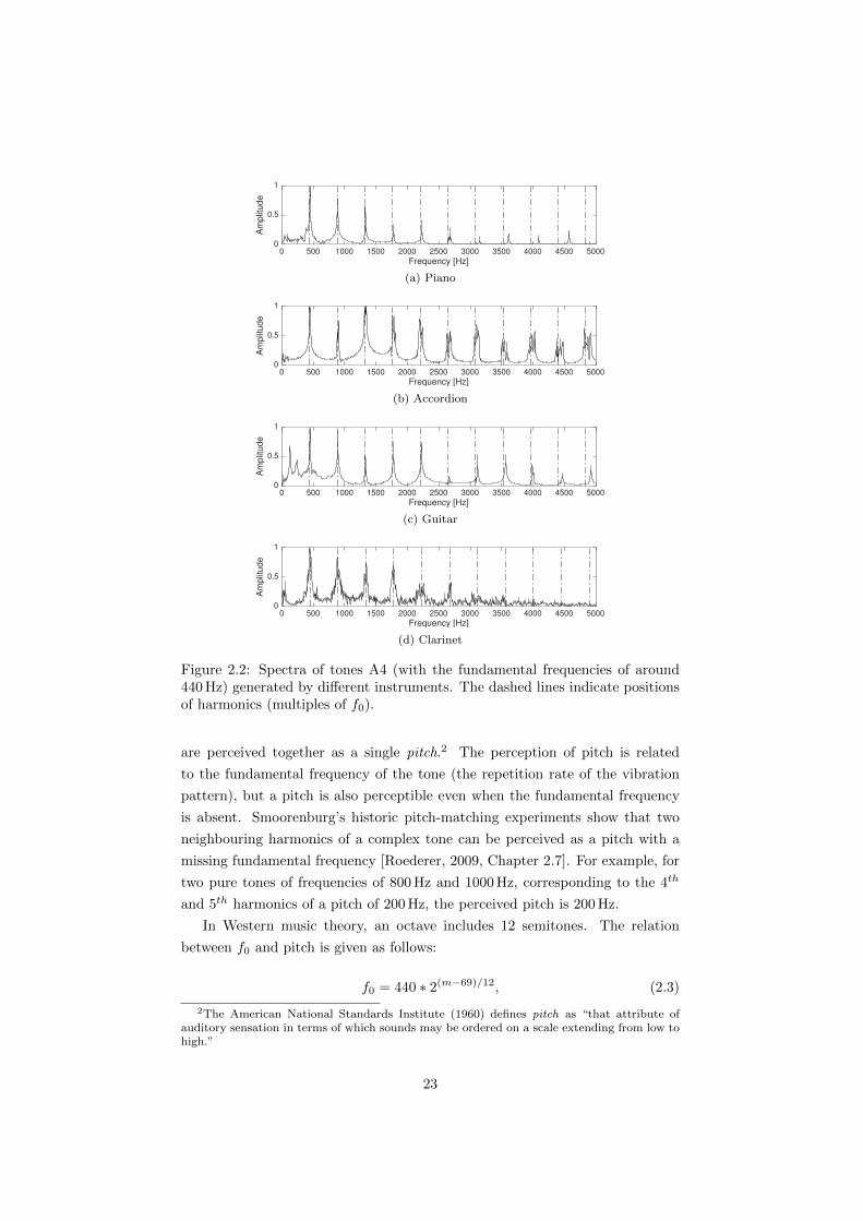
2.2 Spectra of tones A4 (with the fundamental frequencies of around
440Hz) generated by di↵erent instruments. The dashed lines
indicate positions of harmonics (multiples of f0). . . . . . . . . . 23
2.3 Grand piano structure, http://www.radfordpiano.com/structure/ 25
2.4 Time evolution of the spectrum of note A4 (440Hz). . . . . . . . 27
2.5 Di↵erent decay patterns of partials from notes (a) F1 (43.7Hz),
(b) G[2 (92.5Hz) and (c) A1 (55Hz). The top and middle panes
show the waveforms and spectrograms, respectively. The bottom
panes show the decay of selected partials, which are indicated by
the arrows on the spectrograms. The dashed lines are estimated
by the model in Chapter 4. . . . . . . . . . . . . . . . . . . . . . 28
2.6 Dynamic Bayesian Network structure with three layers of vari-
ables: the hidden chords Ct and note combinations Nt, and ob-
served salience St . . . . . . . . . . . . . . . . . . . . . . . . . . . 37
2.7 The hybrid architecture of the AMT systems in [Sigtia et al.,
2015, 2016]. . . . . . . . . . . . . . . . . . . . . . . . . . . . . . . 38
2.8 A general framework for NMF-based transcription. . . . . . . . . 44
2.9 The waveform and spectrogram of a tone with f0 of 440Hz. . . . 49
2.10 Spectral bases and activations obtained using di↵erent cost func-
tions. . . . . . . . . . . . . . . . . . . . . . . . . . . . . . . . . . . 50
3.1 Box-and-whisker plots of (a) accuracy; (b) onset-only F-measure;
and (c) onset-o↵set F-measure; for the Bach10 dataset. . . . . . . 70
4.1 (a) Partial frequencies of note A1 (55Hz), (b) Inharmonicity co-
e�cient B along the whole compass estimated for the piano of
the RWC dataset. . . . . . . . . . . . . . . . . . . . . . . . . . . . 76
8
4.2 Linear fitting for: (a) the 3rd partial of note D1 (f0 = 36.7Hz);
(b) the 2nd partial of note A[1 (f0 = 51.9Hz); (c) the 30th partial
of note D[2 (f0 = 69.3Hz). . . . . . . . . . . . . . . . . . . . . . 78
4.3 Multi-phase linear fitting for: (a) the 7th partial of note B[0
(f0 = 29.1Hz); (b) the 4th partial of note B[2 (f0 = 116.5Hz);
(c) the 1st partial of note E5 (f0 = 659.3Hz). . . . . . . . . . . . 79
4.4 Non-linear curve fitting for: (a) the 22nd partial of note D[1
(f0 = 34.6Hz); (b) the 10th partial of note G1 (f0 = 49Hz); and
(c) the 10th partial of note A1 (f0 = 55Hz). . . . . . . . . . . . . 80
4.5 Flowchart of partial decay modelling. . . . . . . . . . . . . . . . . 82
4.6 Average R2 of di↵erent note groups. f, m, p stand for dynamics,
while L and 3 indicate the linear and mixed models, respectively.
The order of labels in the legend corresponds to the order of lines
from top to bottom. . . . . . . . . . . . . . . . . . . . . . . . . . 83
4.7 Decay response: decay rates against frequency. Lower values
mean faster decay. The greyscale is used to indicate fundamental
frequency, with darker colours corresponding to lower pitches. . . 84
4.8 Decay rates for the first five partials for di↵erent dynamics . . . 86
5.1 An example of output from the proposed model. . . . . . . . . . 88
5.2 An example illustrating of the proposed model (note D3 with the
MIDI index of 50). . . . . . . . . . . . . . . . . . . . . . . . . . . 91
5.3 Example of onset detection showing how activations are processed. 94
5.4 Costs and segments for pitch F3 (MIDI index 53). . . . . . . . . 95
5.5 Attack envelopes. . . . . . . . . . . . . . . . . . . . . . . . . . . . 99
5.6 Detected onsets with di↵erent sparsity for pitch G4 (MIDI index
67). . . . . . . . . . . . . . . . . . . . . . . . . . . . . . . . . . . 101
5.7 Performance using di↵erent sparsity factors and thresholds. The
sparsity factors are indicated by di↵erent shapes, as shown in the
legends. Lines connecting di↵erent shapes are results achieved via
the same threshold. The threshold of the top-left set is �40dB,
and the bottom-right set is �21dB. The dashed lines show F-
measure contours, with the values decreasing from top-right to
bottom-left. . . . . . . . . . . . . . . . . . . . . . . . . . . . . . . 102
5.8 Examples of repeated note detection for low (left) and high (right)
pitches at three dynamic levels. Detected onsets are shown as
brown impulses, and ground truth onsets as red. . . . . . . . . . 109
5.9 Attack envelopes of di↵erent dynamics. . . . . . . . . . . . . . . . 110
5.10 Decay rates as a function of pitch for di↵erent dynamics. . . . . . 111
9
6.1 Spectra of the signal in Equation 6.1 . . . . . . . . . . . . . . . . 116
6.2 The response of a Gaussian window . . . . . . . . . . . . . . . . 117
6.3 Spectrograms and extracted parameters: templates, activations
and spectral widths for notes of di↵erent pitches . . . . . . . . . 120
6.4 Trained spectral widths. . . . . . . . . . . . . . . . . . . . . . . . 121
6.5 Box-and-whisker plots of spectral widths (below 20 frequency
bins) at onsets, with pitch in MIDI index on the vertical axis. . . 125
6.6 Box-and-whisker plots of spectral widths (below 20 frequency
bins) in decay stages, with pitch in MIDI index on the vertical
axis. . . . . . . . . . . . . . . . . . . . . . . . . . . . . . . . . . . 126
6.7 An example of the spectral width and activation for one pitch
during the first 6 seconds of the piece ‘alb se2’. . . . . . . . . . . 127
7.1 Filters for modelling the frequency response di↵erence between
two pianos. . . . . . . . . . . . . . . . . . . . . . . . . . . . . . . 134
10
List of Tables
2.1 Three levels of music dynamics, adapted from [Rossing, 1990,
p. 100] . . . . . . . . . . . . . . . . . . . . . . . . . . . . . . . . . 26
2.2 The usage of the �-divergences in AMT . . . . . . . . . . . . . . 47
2.3 Relation between divergences and generative models, adapted
from [Smaragdis et al., 2014] . . . . . . . . . . . . . . . . . . . . 57
2.4 Public evaluation results on frame-wise accuracy (Accf ) and onset-
only note-level F-measure Fon . . . . . . . . . . . . . . . . . . . . 61
3.1 Note ranges (in MIDI index) of instruments, adapted from Bene-
tos and Dixon [2012b]. . . . . . . . . . . . . . . . . . . . . . . . . 66
3.2 Multiple F0 estimation results (see Section 2.4 for explanation of
symbols). . . . . . . . . . . . . . . . . . . . . . . . . . . . . . . . 69
3.3 Note-tracking results . . . . . . . . . . . . . . . . . . . . . . . . . 70
3.4 Instrument assignment results . . . . . . . . . . . . . . . . . . . . 72
4.1 Average R2 of the linear and mixed models. NP is the number
of partials above the noise level for each dynamic level. . . . . . . 82
5.1 Variable list . . . . . . . . . . . . . . . . . . . . . . . . . . . . . . 90
5.2 Datasets used in the experiments . . . . . . . . . . . . . . . . . . 98
5.3 Experimental configuration for the training stage . . . . . . . . . 98
5.4 Experimental configuration I for the transcription experiments in
Section 5.2.2. . . . . . . . . . . . . . . . . . . . . . . . . . . . . . 99
5.5 Note tracking results with di↵erent fixed sparsity factors (above)
and annealing sparsity factors (below). . . . . . . . . . . . . . . . 100
5.6 Note tracking results (onset-o↵set) and frame-wise results . . . . 103
5.7 Comparison of transcription results with two state-of-the-art meth-
ods on three public datasets. . . . . . . . . . . . . . . . . . . . . 105
5.8 Experimental configuration II for test on repeated notes in Sec-
tion 5.2.4. . . . . . . . . . . . . . . . . . . . . . . . . . . . . . . . 106
11

5.9 Note tracking (onset-only) results for repeated notes in di↵erent
dynamics. . . . . . . . . . . . . . . . . . . . . . . . . . . . . . . . 108
6.1 Comparison of the proposed systems with a standard NMF . . . 123
12
List of Abbreviations
AMT Automatic Music TranscriptionARMA AutoRegressive Moving AverageCQT Constant-Q TransformDAEM Deterministic Annealing Expectation-MaximizationEM Expectation-MaximizationERB Equivalent Rectangular BandwidthHMM Hidden Markov ModelHTC Harmonic Temporal Structure ClusteringHTTC Harmonic Temporal Timbral ClusteringIS Itakura-SaitoKL Kullback-LeiblerMIDI Musical Instrument Digital InterfaceMIR Music Information RetrievalML Maximum LikelihoodNMF Non-negative Matrix FactorizationPLCA Probabilistic Latent Component AnalysisSI-PLCA Shift-Invariant Probabilistic Latent Component AnalysisSTFT Short-Time Fourier TransformSVM Support Vector Machine
13

Chapter 1
Introduction
This thesis explores piano acoustics for automatic transcription, using knowl-
edge and techniques from signal processing, machine learning, and the physics
of musical instruments. Signal processing provides a time-frequency representa-
tion as the front-end of the transcription system and machine learning helps us
estimate the specific parameters for our models that relate the time-frequency
representation to musical notes. The physics of musical instruments, and piano
acoustics in particular, provides us with knowledge about the structure of piano
sounds, and informs our research into new features to improve transcription
accuracy.
Automatic music transcription (AMT) is important because the transcribed
music notation (musical score) is a convenient summarisation of music that al-
lows musicians to e�ciently exchange musical ideas and play them. It can be
used in many applications, such as karaoke, query by humming (e.g. midomi1)
and music education [Tambouratzis et al., 2008]. In order to limit the scope of
the thesis, we decided to focus on a single instrument. Being one of the most
commonly-used instruments, the piano was the natural choice. Piano sounds
have many specific features, including either ones simplifying the transcription
task like discrete frequency and percussive onsets, or others such as time-varying
timbre, large frequency and dynamic ranges. The richness of piano sounds
makes the topic (piano transcription) interesting to explore. Furthermore, pi-
ano acoustics have been well investigated, providing us with ample theoretical
findings which we can make use of.
In order to transcribe piano music signals into a symbolic representation,
we make use of the non-negative matrix factorisation (NMF) framework to gen-
erate transcription systems motivated by piano acoustics. The thesis does not
use methods such as simpler template matching, neural networks and hidden
1http://www.midomi.com
14
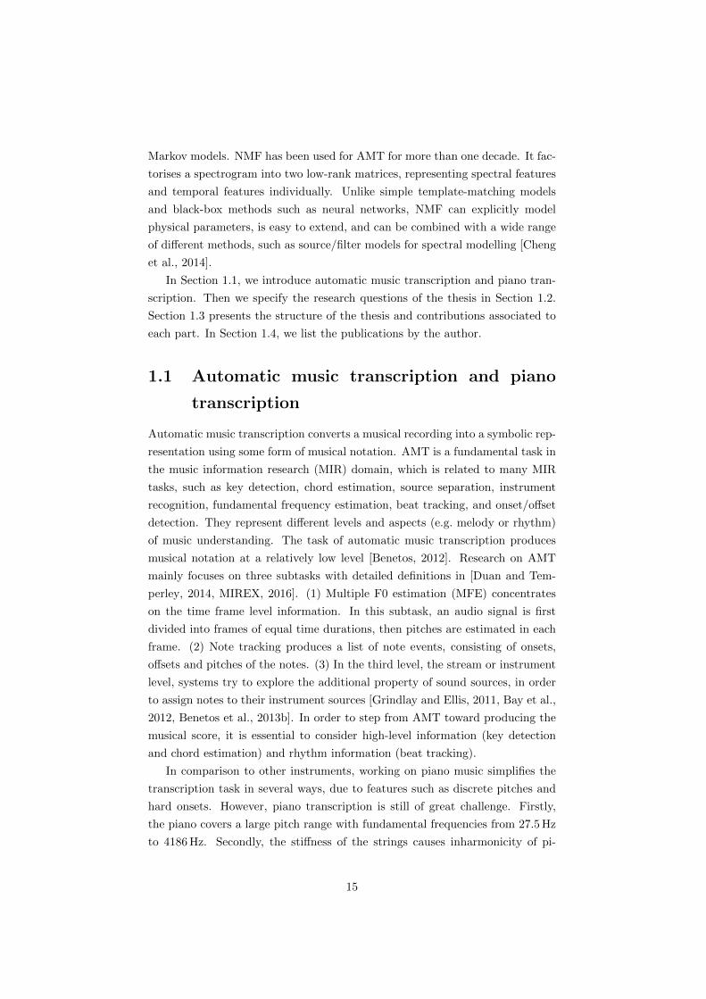
Markov models. NMF has been used for AMT for more than one decade. It fac-
torises a spectrogram into two low-rank matrices, representing spectral features
and temporal features individually. Unlike simple template-matching models
and black-box methods such as neural networks, NMF can explicitly model
physical parameters, is easy to extend, and can be combined with a wide range
of di↵erent methods, such as source/filter models for spectral modelling [Cheng
et al., 2014].
In Section 1.1, we introduce automatic music transcription and piano tran-
scription. Then we specify the research questions of the thesis in Section 1.2.
Section 1.3 presents the structure of the thesis and contributions associated to
each part. In Section 1.4, we list the publications by the author.
1.1 Automatic music transcription and piano
transcription
Automatic music transcription converts a musical recording into a symbolic rep-
resentation using some form of musical notation. AMT is a fundamental task in
the music information research (MIR) domain, which is related to many MIR
tasks, such as key detection, chord estimation, source separation, instrument
recognition, fundamental frequency estimation, beat tracking, and onset/o↵set
detection. They represent di↵erent levels and aspects (e.g. melody or rhythm)
of music understanding. The task of automatic music transcription produces
musical notation at a relatively low level [Benetos, 2012]. Research on AMT
mainly focuses on three subtasks with detailed definitions in [Duan and Tem-
perley, 2014, MIREX, 2016]. (1) Multiple F0 estimation (MFE) concentrates
on the time frame level information. In this subtask, an audio signal is first
divided into frames of equal time durations, then pitches are estimated in each
frame. (2) Note tracking produces a list of note events, consisting of onsets,
o↵sets and pitches of the notes. (3) In the third level, the stream or instrument
level, systems try to explore the additional property of sound sources, in order
to assign notes to their instrument sources [Grindlay and Ellis, 2011, Bay et al.,
2012, Benetos et al., 2013b]. In order to step from AMT toward producing the
musical score, it is essential to consider high-level information (key detection
and chord estimation) and rhythm information (beat tracking).
In comparison to other instruments, working on piano music simplifies the
transcription task in several ways, due to features such as discrete pitches and
hard onsets. However, piano transcription is still of great challenge. Firstly,
the piano covers a large pitch range with fundamental frequencies from 27.5Hz
to 4186Hz. Secondly, the sti↵ness of the strings causes inharmonicity of pi-
15
ano sounds. Thirdly, the number of simultaneous notes can be high in piano
music. It is even possible to have over 10 notes at the same time (using the sus-
tain pedal). Lastly, the decaying note energy makes the o↵sets hard to detect
correctly.
In this thesis, we start our studies on automatic music transcription in Chap-
ter 3, in which we analyse results of AMT systems at all three levels (frame level,
note level and instrument level). After investigating piano decay in Chapter 4,
we focus on piano transcription in Chapter 5 and 6, so that instrument assign-
ment is not needed for these two chapters.
1.2 Research questions
The work in this thesis addresses one main research question (RQ), which we
then break down into four more specific questions as detailed below.
RQ: Can automatic transcription of piano music be improved by con-
sidering acoustical features of the piano?
This thesis targets the automatic transcription task on a specific piano. Given
the situation that we have access to isolated notes produced by the piano (the
training dataset), we want to know what we can learn from the training dataset,
and how that might be useful for transcribing polyphonic music pieces played
on the same piano.
In order to answer the research question, we review both piano acoustics
and automatic music transcription methods. The thesis is undertaken from the
following four aspects.
RQ1: What are the weaknesses of matrix factorisation-based ap-
proaches and how can the weaknesses be addressed?
We review automatic music transcription systems in Sectoin 2.2. Among the
methods, non-negative matrix factorisation (NMF) is commonly used since
[Smaragdis and Brown, 2003]. NMF can represent the spectral features and
temporal features of musical tones individually, is easy to extend, and has been
used in a physics-informed piano analysis system [Rigaud, 2013]. NMF is cho-
sen as the fundamental framework for the proposed methods in this thesis. We
specify systems based on non-negative matrix factorisation in Section 2.3, and
deal with the local minimum problem of probabilistic latent component analysis
(PLCA) (the probabilistic counterpart of NMF) in Chapter 3.
16
RQ2: Which features can we learn associated with piano acoustics?
Piano acoustics studies features associated with the physical structure and ex-
citation mechanism of the piano. We briefly introduce piano acoustics in Sec-
tion 2.1.2, including inharmonicity, attack noise and temporal evolution of piano
tones. Inharmonicity has been studied by Rigaud [2013] for piano transcription
and tuning. This thesis will focus on the time-varying spectral structures and
the temporal evolution of piano tones.
RQ3: How do piano partials decay in real recordings?
Among the features associated to piano acoustics, we are particularly interested
in piano decay. The theory of piano decay was studied by Weinreich [1977]
and has been applied for sound synthesis [Aramaki et al., 2001, Bensa et al.,
2003, Bank, 2000, 2001, Lee et al., 2010]. Previous studies on decay parameter
estimation were only verified on some examples of synthetic notes [Valimaki
et al., 1996, Karjalainen et al., 2002]. We do not know how well the theory
based on two coupled strings works for all piano tones with di↵erent numbers of
strings (1-3 strings). In Chapter 4, we track the decay of acoustic piano tones to
understand partial decay of all 88 piano notes. We analyse the influence of the
frequency range, pitch range and dynamic on decay patterns, to gain insights
into how the decay information can be used in piano transcription systems.
RQ4: How can acoustical features be modelled in transcription sys-
tems?
Piano acoustics is well understood, but it is not intuitive to analyse and apply
the acoustical features in an NMF framework. Previous studies on analysing mu-
sical signals using NMF are undertaken in several ways [Rigaud, 2013, Cheng
et al., 2014], in which the parametric models attracted our attention. Hen-
nequin et al. [2011a] extend the temporal activations of a standard NMF to
be frequency-dependent by using the auto-regressive moving average (ARMA)
model. Then the parameters of the ARMA model can be estimated directly.
Hennequin et al. [2010] and Rigaud [2013] parameterise each partial by its fre-
quency and the main lobe of the Hamming window, to estimate the frequencies
directly for vibratos and inharmonic tones, respectively. In Chapter 5, we pa-
rameterise the decay envelope as an exponentially decaying function. In Chap-
ter 6, we model each partial by its frequency and a Gaussian function, with the
spectral width represented by the standard deviation of the Gaussian function.
Then we can model and directly estimate the decay rate and the spectral width
respectively in these proposed parametric models.
17

1.3 Thesis structure and contributions
The remainder of this thesis is organised as follows, with the associated contri-
butions of the chapters.
Chapter 2 - Background: We present necessary information on piano mu-
sic and computational methods. First, we introduce sound generation
and perception, and specify piano acoustics as the theoretical foundation
of our proposed piano transcription systems. Then we give a literature
review on related work in the automatic music transcription (AMT) do-
main. Especially, we present a general framework for AMT systems based
on non-negative matrix factorisation (NMF), including front-end, post-
processing of standard AMT systems, and parameter estimation methods
and constraints imposed in the NMF framework. Finally we describe com-
monly used evaluation metrics and compare the performance of important
methods based on the results of a public evaluation platform.
Chapter 3 - A Deterministic Annealing EM Algorithm for AMT:
We deal with the local minimal problem of PLCA with a Deterministic
Annealing Expectation-Maximisation (DAEM) algorithm and show the
improvements in transcription performance by doing so.
Contributions: We provide modified update rules for a PLCA-based
transcription method [Benetos and Dixon, 2012a] according to the DAEM,
with the introduction of a ‘temperature’ parameter. In comparison to
the baseline method, the proposed method brings improvements to both
frame-level and note-level results.
Chapter 4 - Modelling the Decay of Piano Tones: We track the decay
of acoustic piano tone. First, partials are found with inharmonicity con-
sidered. Then we track each partial to understand the decay of piano
tones in real recordings.
Contributions: We track the decay of acoustic piano tones from the
RWC Music Database in detail (first 30 partials of 88 notes played in 3
dynamics). We compare the temporal decay of individual piano partials to
the theoretical decay patterns based on piano acoustics [Weinreich, 1977].
We analyse the influence of the frequency range, pitch range and dynamic
on decay patterns, and gain insights into how piano transcription systems
can make use of decay information.
Chapter 5 - An Attack/Decay Model for Piano Transcription: We
propose an attack/decay model motivated by piano acoustics, which
models the time-varying timbre and decaying energy of piano notes. We
18

detect note onsets by peak-picking on attack activations, then o↵sets for
each pitch individually based on the reconstruction errors.
Contributions: The attack/decay method brings three refinements to
the non-negative matrix factorisation: (1) introduction of attack and har-
monic decay components; (2) use of a spike-shaped note activation that
is shared by these components; (3) modelling the harmonic decay with an
exponential function.
The results show that piano transcription performance for a known piano
can be improved by explicitly modelling piano acoustical features. In
addition, the proposed methods help to automatically analyse the decay
of piano sounds in di↵erent dynamic levels.
Chapter 6 - Modelling Spectral Widths for Piano Transcription: We
present a model for piano notes with time-varying spectral widths in an
NMF framework. We refine detected onsets by their spectral widths, and
analyse the spectral widths of isolated notes and notes in the musical
pieces.
Contributions: We present a new feature, the spectral width, which
could be potentially used as a cue to indicate the duration of piano notes.
The results on isolated notes suggest that the spectral width is large in
the attack part, then it decreases and remains stable in the decay part.
We use the spectral widths to refine detected onsets in the transcription
experiment. We analyse the spectral width distributions at onsets and in
the decay parts for notes in the musical pieces and show several directions
of future work.
Chapter 7 - Conclusions and further work: This chapter summarises the
contributions of the thesis and provides a few directions worthy of further
investigation, building on the work in the main chapters and generalising
the proposed models for other pianos and instruments.
1.4 Related publications
The publications listed below are closely related to this thesis. The main chap-
ters are based on [5] (Chapter 3), [3] (Chapter 4) and [1] (Chapter 5), respec-
tively. The author was the main contributor to the listed publications, who
performed all scientific experiments and manuscript writing, under supervision
of SD and MM. Co-authors SD, MM, EB provided advice during meetings and
comments on manuscripts. EB provided code of the baseline model in [5] and
[6].
19

Peer-reviewed conference papers
[1] T. Cheng, M. Mauch, E. Benetos and S. Dixon. An attack/decay model for
piano transcription. In 17th International Society for Music Information
Retrieval Conference (ISMIR), pages 584-590, 2016.
[2] T. Cheng, S. Dixon and M. Mauch. Improving piano note tracking by
HMM smoothing. In European Signal Processing Conference (EUSIPCO),
pages 2009-2013, 2015.
[3] T. Cheng, S. Dixon and M. Mauch. Modelling the decay of piano sounds.
In IEEE International Conference on Acoustics, Speech, and Signal Pro-
cessing (ICASSP), pages 594-598, 2015.
[4] T. Cheng, S. Dixon and M. Mauch. A comparison of extended source-filter
models for musical signal reconstruction, In International Conference on
Digital Audio E↵ects (DAFx), pages 203-209, 2014.
[5] T. Cheng, S. Dixon and M. Mauch. A deterministic annealing EM algo-
rithm for automatic music transcription. In 14th International Society for
Music Information Retrieval Conference (ISMIR), pages 475-480, 2013.
Other publication
[6] T. Cheng, S. Dixon and M. Mauch. MIREX submission: A determin-
istic annealing EM algorithm for automatic music transcription. Music
Information Retrieval Evaluation eXchange (MIREX), 2013.
20
Chapter 2
Background
The scope of this thesis is the automatic transcription of audio recordings of
piano music into symbolic notation. It relates to piano music and computational
methods. In this chapter, we present necessary information from both aspects.
First, we introduce related music knowledge in Section 2.1. Then in Section 2.2
we give a literature review on related work in the automatic music transcription
(AMT) domain. In Section 2.3 we focus on techniques for AMT systems based
on non-negative matrix factorisation (NMF). Section 2.4 describes commonly
used evaluation metrics. In Section 2.5 we conclude this chapter.
2.1 Music knowledge
We first introduce how sounds are generated and how people perceive them in
Section 2.1.1, to understand the observation (input) and expected output of
AMT systems. Secondly, in Section 2.1.2 we specify piano acoustics: features
related to the piano’s physical structure, which is the theoretical fundament of
our proposed piano transcription systems.
2.1.1 Sound generation and perception
In this section, we discuss sounds of music instruments generated via vibrating
strings or air columns (pitched instruments).
Given a tense string with fixed ends, when the string is set to vibrate, it
excites a series of waves with nodes at both ends of the string, as shown in
Figure 2.1. These waves are the standing waves of the string; a detailed demon-
stration can be found online.1 The frequency of the first wave is called the
fundamental frequency (f0) of the string. Compared to the string length L, the
1http://newt.phys.unsw.edu.au/jw/strings.html
21
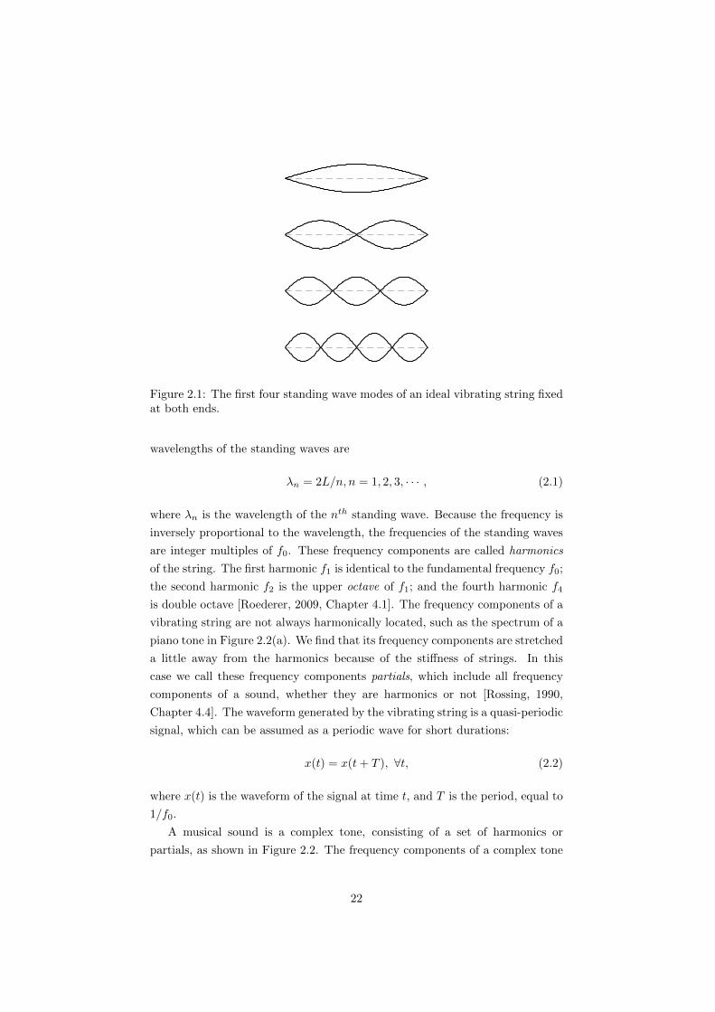
Figure 2.1: The first four standing wave modes of an ideal vibrating string fixedat both ends.
wavelengths of the standing waves are
�n = 2L/n, n = 1, 2, 3, · · · , (2.1)
where �n is the wavelength of the nth standing wave. Because the frequency is
inversely proportional to the wavelength, the frequencies of the standing waves
are integer multiples of f0. These frequency components are called harmonics
of the string. The first harmonic f1 is identical to the fundamental frequency f0;
the second harmonic f2 is the upper octave of f1; and the fourth harmonic f4
is double octave [Roederer, 2009, Chapter 4.1]. The frequency components of a
vibrating string are not always harmonically located, such as the spectrum of a
piano tone in Figure 2.2(a). We find that its frequency components are stretched
a little away from the harmonics because of the sti↵ness of strings. In this
case we call these frequency components partials, which include all frequency
components of a sound, whether they are harmonics or not [Rossing, 1990,
Chapter 4.4]. The waveform generated by the vibrating string is a quasi-periodic
signal, which can be assumed as a periodic wave for short durations:
x(t) = x(t+ T ), 8t, (2.2)
where x(t) is the waveform of the signal at time t, and T is the period, equal to
1/f0.
A musical sound is a complex tone, consisting of a set of harmonics or
partials, as shown in Figure 2.2. The frequency components of a complex tone
22
0 500 1000 1500 2000 2500 3000 3500 4000 4500 5000Frequency [Hz]
0
0.5
1
Am
plit
ude
(a) Piano
0 500 1000 1500 2000 2500 3000 3500 4000 4500 5000Frequency [Hz]
0
0.5
1
Am
plit
ude
(b) Accordion
0 500 1000 1500 2000 2500 3000 3500 4000 4500 5000Frequency [Hz]
0
0.5
1
Am
plit
ude
(c) Guitar
0 500 1000 1500 2000 2500 3000 3500 4000 4500 5000Frequency [Hz]
0
0.5
1
Am
plit
ude
(d) Clarinet
Figure 2.2: Spectra of tones A4 (with the fundamental frequencies of around440Hz) generated by di↵erent instruments. The dashed lines indicate positionsof harmonics (multiples of f0).
are perceived together as a single pitch.2 The perception of pitch is related
to the fundamental frequency of the tone (the repetition rate of the vibration
pattern), but a pitch is also perceptible even when the fundamental frequency
is absent. Smoorenburg’s historic pitch-matching experiments show that two
neighbouring harmonics of a complex tone can be perceived as a pitch with a
missing fundamental frequency [Roederer, 2009, Chapter 2.7]. For example, for
two pure tones of frequencies of 800Hz and 1000Hz, corresponding to the 4th
and 5th harmonics of a pitch of 200Hz, the perceived pitch is 200Hz.
In Western music theory, an octave includes 12 semitones. The relation
between f0 and pitch is given as follows:
f0 = 440 ⇤ 2(m�69)/12, (2.3)
2The American National Standards Institute (1960) defines pitch as “that attribute ofauditory sensation in terms of which sounds may be ordered on a scale extending from low tohigh.”
23
where m is the Musical Instrument Digital Interface (MIDI) index of a pitch.
For a piano, the pitch range is m 2 [21, 108].
The sounds in Figure 2.2 have the same pitch. However, their spectra vary.
The spectral structure of a pitched sound is characterised by the excitation
mechanism and physical structure of the instrument [Roederer, 2009, Chap-
ter 4.2, 4.3]. The identification of the instrument is related to timbre3 percep-
tion, which depends primarily on the precise structure of the spectrum, as stud-
ied in psychoacoustic experiments in [Plomp, 1970, 1976, McAdams, 1999]. For
example, a musician may describe a tone as dull or stu↵y (few upper harmon-
ics), “nasal” (mainly odd harmonics), bright or sharp (many enhanced upper
harmonics), or otherwise. These qualifications are associated to actual instru-
mental tones (fluty, stringy, reedy, brassy, etc.) [Roederer, 2009, Chapter 4.8].
In this section, we briefly introduce how a pitched sound is generated with
harmonics (partials) and what is primary to human perception of the pitch and
timbre of the sound. Just like human perception of music, an automatic music
transcription (AMT) system also works on a waveform of complex tones, to
estimate the pitch of each tone. The expected output can be in the form of a
time-pitch representation or a list of note events.
2.1.2 Piano acoustics
In this section we investigate piano acoustics, specific properties of sounds as-
sociated to piano physics.
A piano mainly consists of a keyboard, keys, hammers, strings and a sound-
board, as shown in Figure 2.3. It has 88 keys, with a pitch range of more than 7
octaves (A0 to C8), covering fundamental frequencies from 27.5Hz to 4186Hz.
Each piano tone is generated by the string(s) vibrating at a specific frequency.
The fundamental frequency of a string with fixed ends is given by [Pierce, 1983,
Chapter 2]:
f =1
2l
sT
µ. (2.4)
It is related to the length l, the tension T and the linear density µ (mass per
unit length) of the string. This means that for two tones an octave apart, the
string length of the lower pitch is twice as long as that of the higher pitch, if
the strings have equal tension and density. In this case, the string lengths of
low-pitch keys would be too long to fit on the sound board. To build a piano
of reasonable size, low bass tones usually use thicker strings, and treble tones
(tones in the high pitch range) use thinner strings with higher tensions [Burred,
3The American National Standards Institute (1960) defines timbre as “that attribute ofauditory sensation in terms of which a listener can judge two sounds similarly presented andhaving the same loudness and pitch as dissimilar.”
24

Figure 2.3: Grand piano structure, http://www.radfordpiano.com/structure/
2004], [Fletcher and Rossing, 1998, Chapter 12]. The short and thin strings are
less resonant than the long and thick strings, therefore, two or three strings are
used for a mid or high pitch to produce a louder sound [Livelybrooks, 2007].
Due to the sti↵ness of the string, partials of piano tones are slightly stretched
away from the harmonic positions (shown in Figure 2.2(a)), which is referred
to as inharmonicity. The inharmonicity coe�cient B is calculated as follows
[Fletcher et al., 1962]:
B =⇡3Qd4
64l2T, (2.5)
where Q is Young’s modulus, d is the diameter of the string, l and T are the
length and the tension of the string. This shows that the degree of inharmonic-
ity increases with decreased length and increased thickness. Then piano tones
of low-pitch and high-pitch ranges have greater inharmonicity than mid-pitch
tones. Experiments in the 1960’s showed that slight inharmonicity made syn-
thesised piano tones sound more natural, and was one of the characteristics that
added certain warmth [Fletcher et al., 1962], richness and quality to the piano
sound [Blackham, 1965]. However, the sound quality can be influenced nega-
tively by excessive inharmonicity [Burred, 2004, Chaigne and Kergomard, 2016].
Especially for bass notes, when the partials are very inharmonic, the pitch can
be confusing with a less pleasing sound. In an experiment on the audibility of
25

Table 2.1: Three levels of music dynamics, adapted from [Rossing, 1990, p. 100]
Name Symbol Meaning
forte f Loudmezzo forte mf Moderately loudpiano p Soft
inharmonicity [Jarvelainen et al., 2001], inharmonicity was more easily detected
for bass tones than treble tones.
Inharmonicity also influences piano tuning [Schuck and Young, 1943]. When
tuning a piano, a note’s upper octave is tuned to the frequency of its second
partial to eliminate the beats between these two notes. Then the fundamental
frequency ratio of an octave is slightly larger than 2. This results in the stretched
piano tuning, which allows the piano to sound maximally in tune with itself. In
[Rigaud, 2013], a model is proposed and studied, to explain inharmonicity and
tuning.
An individual piano tone is generated by the hammer hitting the string(s)
of the key. There are three characteristics of piano sounds associated with
the attack motion [Meyer, 2009, Chapter 3.4]. Firstly, the strike produces a
percussive sound. We can see that the energy distribution is flatter at the
attack stage, as shown in Figure 2.4. Secondly, the dynamics of a piano tone
are primarily determined by the force of the key attack [Hirschkorn, 2004].
Commonly used dynamics symbols are introduced in Table 2.1. Thirdly, the
hammer hits the string at 1/7 of its whole length, resulting in a particular
excitation structure with suppressed 7th, 14th, ..., partials.
Then we look at the sound evolution after the attack. In a grand piano the
string is excited into a perpendicular motion to the soundboard because the
hammer strikes from below. This perpendicular motion decays quickly. Due
to the coupling of the bridge and soundboard, the plane of vibration gradually
rotates to a parallel motion which decays more slowly [Weinreich, 1977]. This is
referred to as the typical “double decay” of the piano, as shown in Figure 2.5(a).
In a piano, most notes have more than one string per note. Usually only the
lowest ten or so notes have one string per note. The subsequent (about 18)
notes have two strings, and the rest have three strings. For notes with multiple
strings, the decay rate will double or treble if the strings are tuned to exactly
the same frequency. To make the sound sustain longer, the strings are tuned
to slightly di↵erent frequencies. Weinreich [1977] studies the coupled oscillation
of two strings in detail. If the frequency di↵erence between strings is small,
the coupled motion will result in a double decay, as shown in Figure 2.5(b).
26
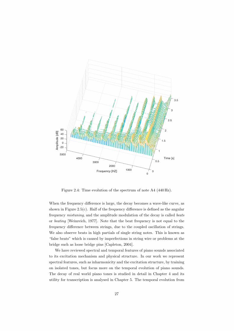
Figure 2.4: Time evolution of the spectrum of note A4 (440Hz).
When the frequency di↵erence is large, the decay becomes a wave-like curve, as
shown in Figure 2.5(c). Half of the frequency di↵erence is defined as the angular
frequency mistuning, and the amplitude modulation of the decay is called beats
or beating [Weinreich, 1977]. Note that the beat frequency is not equal to the
frequency di↵erence between strings, due to the coupled oscillation of strings.
We also observe beats in high partials of single string notes. This is known as
“false beats” which is caused by imperfections in string wire or problems at the
bridge such as loose bridge pins [Capleton, 2004].
We have reviewed spectral and temporal features of piano sounds associated
to its excitation mechanism and physical structure. In our work we represent
spectral features, such as inharmonicity and the excitation structure, by training
on isolated tones, but focus more on the temporal evolution of piano sounds.
The decay of real world piano tones is studied in detail in Chapter 4 and its
utility for transcription is analysed in Chapter 5. The temporal evolution from
27

0 1 2−0.50
0.5(a)
Ampl
itude
Freq
uenc
y (k
Hz)
0.5 1 1.50
0.5
1
1.5
0 1 2−40
−30
−20
−10
0
Time (s)
Ener
gy (d
B)
0 1 2−0.50
0.5(b)
0.5 1 1.50
0.5
1
1.5
0 1 2−60
−40
−20
0
Time (s)
0 1 2−0.50
0.5(c)
0.5 1 1.50
0.5
1
1.5
0 1 2−80
−60
−40
−20
0
Time (s)
ObservationModel
ObservationModel
ObservationModel
Figure 2.5: Di↵erent decay patterns of partials from notes (a) F1 (43.7Hz),(b) G[2 (92.5Hz) and (c) A1 (55Hz). The top and middle panes show thewaveforms and spectrograms, respectively. The bottom panes show the decayof selected partials, which are indicated by the arrows on the spectrograms. Thedashed lines are estimated by the model in Chapter 4.
the attack to decay stage is modelled in Chapter 6.
2.2 Related work
In this section, we review methods proposed for automatic music transcription.
Readers are referred to [Klapuri and Davy, 2006, de Cheveigne, 2006, Chris-
tensen and Jakobsson, 2009, Benetos et al., 2013b] for some excellent literature
reviews. Here we provide a new aspect to catalogue the methods by the level
of music understanding they involve. In the following sections, we introduce
methods automatically transcribing musical signals by relating the pitch of a
musical tone to its fundamental frequency (period), harmonics (partials) and
spectral structure (timbre), modelling musicological information, and making
use of classification-based methods. Then in Section 2.2.6, we cover steps to
form note events and some note-level methods which model the discrete note
events directly.
28

2.2.1 Methods based on periodicity
Methods reviewed in this section detect the pitch of a musical tone by its period.
These methods, which are also referred to as pitch detection algorithms (PDA)
[Hess, 1983, Gerhard, 2003], usually work only for single-pitch detection.
As mentioned in Section 2.1.1, a pitched sound is a quasi-periodic signal and
can be assumed as a periodic wave for short durations. We rewrite Equation 2.2
as follows:
x(t)� x(t+ T ) = 0, 8t, (2.6)
where x(t) is the waveform of the signal, and T is the period, equal to 1/f0.
The key for detecting period is to design a period candidate generating function,
which should have a maximal or minimal value at the time of the period [Talkin,
1995]. Commonly used functions are based on the autocorrelation function
(ACF) [Rabiner, 1977], and the average magnitude di↵erence function (AMDF)
[Ross et al., 1974]. In a frame with an integration window of size W , the ACF
at time index t is defined as:
ACF t(⌧) =t+WX
j=t+1
x(j)x(j + ⌧), (2.7)
where ⌧ is the time lag. We show the squared-di↵erence function (SDF)
[de Cheveigne, 1998], a variant of AMDF, defined as:
SDF t(⌧) =t+WX
j=t+1
(x(j)� x(j + ⌧))2. (2.8)
The cepstrum is also a commonly used method for period detection, which
is defined as the inverse Fourier transform of the short-time log magnitude
spectrum [Noll, 1967, Oppenheim and Schafer, 2004]. Unlike the previous time-
domain method, the cepstrum is performed in the frequency-domain, then in-
versely transformed back to the time domain. The harmonic peaks are flattened
by the log operator on the magnitude spectrum.
The above methods show peaks or valleys at multiples of the period, with the
period detected by the first peak of the ACF and cepstrum or first valley of the
AMDF and SDF. Associating the pitch with the zero-lag peak and other high-
order peaks are the typical errors in these pitch detection algorithms. Several
extended methods to solve these problems are introduced as follows.
de Cheveigne and Kawahara [2002] propose a method, YIN, based on ACF
with a number of modifications for f0 estimation. The method first computes a
modified ACF with shrunk integration window size, which lowers the high-order
peaks. Then the square di↵erence function is applied as the second indicator.
29

It is argued that the SDF is closer to the representation of the periodic signal
in Equation 2.6, which contributes to a significant reduction of the error rate.
A cumulative mean normalised di↵erence function is proposed based on SDF to
decrease the errors near the zero lag. In the fourth step, an absolute threshold
(0.1) is used to find the first dip for the period. The global minimum is selected
if no dip is below the threshold. Then parabolic interpolation is used for a
better estimation of the period. There is a final smoothing step to reduce
the fluctuation of the f0 estimation. The algorithm outperforms all compared
methods, and is simple and computationally e�cient with few parameters to be
tuned.
McLeod and Wyvill [2005] propose a normalised square di↵erence function
(NSDF) to find the pitch, which is defined as:
NSDF t(⌧) =ACF t(⌧)
mt(⌧)(2.9)
where mt(⌧) =Pt+W
j=t+1 (x(j)2+x(j+⌧)2). This normalised SDF (or normalised
ACF) minimises the edge e↵ects of the decreasing window size. The highest
positive maxima between pairs of zero crossings are selected as the candidates,
and the maximum at delay 0 is ignored. A threshold is set by multiplying the
global maximum with a constant k 2 [0.8, 1). The delay ⌧ of the first candidate
above the threshold is detected as the pitch period. Parabolic interpolation is
also applied to find the positions of the maxima more accurately. The method
uses a small window for a better representation of a changing pitch, such as
vibrato.
The above period detection methods actually find the smallest common pe-
riod shared by all harmonics of a pitch. If there are two pitches, they detect
the smallest common period they share, or a ‘root’ frequency of the two notes
[Moorer, 1975]. So these methods usually work only for single-pitch signals.
In the following, we introduce two methods jointly using temporal and spec-
tral representation [Peeters, 2006, Emiya et al., 2007]. The methods are moti-
vated by the observation of inverse octave errors (‘twice the pitch’ and ‘half the
pitch’) of the two representations. The pitch detection function is a product of
the temporal method and the spectral method, to reduce both octave errors. In
[Peeters, 2006], di↵erent representations are considered: spectral ones include
the Discrete Fourier Transform (DFT) of the signal, the frequency reassignment
(REAS), and the Auto-Correlation Functions of DFT and REAS; and temporal
ones include the Auto-Correlation Function and Real-Cepstrum of the signal.
Then the proposed periodicity function is computed by the product of each of
the two kinds of representations. The method is tested on a large test set of over
5000 musical instrument sounds, showing competitive results in comparison to
30
the YIN estimator [de Cheveigne and Kawahara, 2002].
Emiya et al. [2007] propose a pitch estimation method for a short analysis
window and focusing on piano sounds. Both the temporal method (based on
the autocovariance function) and spectral method (based on spectral matching)
include the inharmonicity factor. The final pitch detection function is a product
of the two methods. This model is the first physics-based transcription system
for piano. The test dataset contains a large set of isolated piano tones for
RWC database [Goto et al., 2003], a PROSONUS and a Yamaha upright piano.
Better performance is achieved by the proposed method compared to the YIN
estimator [de Cheveigne and Kawahara, 2002], especially for low-pitch and high-
pitch notes.
2.2.2 Methods based on harmonics (partials)
We know that a pitched sound actually consists of a set of frequency components,
appearing at or near integer multiplies of f0, as shown in Section 2.1.1. Methods
reviewed in this section make use of harmonics (partials) to detect the pitch of
the sound.
A subharmonic summation method uses the weighted sum of harmonic am-
plitudes [Hermes, 1988]:
H(f) =NX
n=1
hnP (nf), (2.10)
where H(f) is the subharmonic sum spectrum, and hn is the weight for the
nth harmonic. P is the spectrum with low frequency noise suppressed. Pitch is
detected with f0 where H(f) is maximum.
Taking harmonics (partials) into account makes it possible to estimate mul-
tiple pitches. The first attempt for duets was carried out by Moorer [1975].
The method first detects the root frequency (the greatest common frequency)
of the two notes with a periodicity detector. Bandpass filters centred at multi-
ples of the root filter out harmonics of notes. The strongest harmonic and its
sub-harmonics are compared to detect the root. Each integer multiple of the
root forms a note hypothesis. The hypothesis is tested by the existence of its
harmonics.
Klapuri [2003] proposes a multiple fundamental frequency estimation
method by iteratively detecting the predominant pitch and cancelling the de-
tected sound. First, the power spectrum is magnitude-warped and noise is sup-
pressed using a moving average filter. Then for each iteration, an f0 is detected
with the highest global weight. The global weight of an f0 is a sum of its squared
band-wise weights with adopted inharmonicity, and the band-wise weight is a
sum of its partials’ amplitudes modified by a triangular window. The method
31

assumes a smooth spectrum for a pitched tone. When cancelling a detected
pitch, the spectrum of the detected pitch is smoothed to reduce its influence
on remaining pitches. The smoothing method replaces the original amplitude
value of each partial by the weighted mean of the partials’ amplitudes in an
octave-wide triangular weighting window if the weighted mean is smaller. Two
terms based on the signal-to-noise ratio are used to stop the iteration.
Yeh et al. [2010] propose a joint estimation method for multiple fundamen-
tal frequency estimation by progressively combining hypothetical sources and
iteratively verifying each combination. The system first applies an adaptive
noise level estimation to divide the spectral peaks into partials of harmonic
sources and noise. A score function is defined as the weighted sum of the four
criteria, which are proposed to prevent sub-harmonic/super-harmonic errors,
including harmonicity, mean bandwidth, spectral centroid, and the standard
deviation of mean time. The f0 candidates are selected by iteratively applying
a predominant-f0 estimation and cancelling related partials. A harmonically
related f0 (HRF0) of the extracted f0s is also selected as a candidate if it is
dominant and disturbs the envelope smoothness. To infer the best combination,
f0 candidates are added to the combination one by one starting with the highest
score. The newly added f0 is considered valid if it either explains more energy
than the noise, or significantly improves the envelope smoothness for HRF0s.
Duan et al. [2010] estimate multiple f0s by modelling both the spectral
peak and non-peak regions. The peak region likelihood helps find f0s that
have harmonics that explain peaks, and the non-peak region likelihood helps
avoid f0s that have harmonics in the non-peak region. The method first detects
peaks from the spectrum. The f0 candidates are restricted to be around peaks
with the lowest frequencies or (locally) highest amplitudes. To reduce the time
complexity, an iterative greedy search strategy is applied to add f0s one by
one. For each iteration, a set of f0s is found which maximises the product
of the peak and non-peak region likelihoods. The likelihoods are based on the
probabilities of peaks belonging to given f0s, which are learned from monophonic
and polyphonic training data. A threshold-based method is used to end the
iteration. In the post-processing step inconsistent f0 estimates are removed and
the missing f0 is reconstructed using neighbouring f0 estimates.
Dressler [2011] proposes a pitch estimation method based on pair-wise anal-
ysis of spectral peaks. The method first detects amplitude and instantaneous
frequency (IF) of the spectral peaks, with each peak magnitude weighted by
its IF. The method finds pitch candidates by assuming two spectral peaks are
successive harmonics or successive odd harmonics for wind instruments (sup-
pressed even harmonics because of the open end of wind instruments). A pitch
candidate is rated by a multiplication of values of functions indicating the har-
32
monicity, spectral smoothness, attenuation by intermediate peaks and harmonic
impact of the candidate. Each function operates on frequencies or amplitudes
of the pitch pair or peaks between them.
2.2.3 Methods based on timbre
Timbre is associated to the spectrum of the musical sound. It primarily explains
the human ability of distinguishing instruments, as explained in Section 2.1.1.
Methods reviewed in this section represent the spectral structure of each pitch,
with the ability to be applied to multi-instrument music signals to identify
pitches from di↵erent instruments.
All matrix-factorisation-based AMT methods are included in this category,
such as non-negative matrix factorisation (NMF) [Smaragdis and Brown, 2003],
probabilistic latent component analysis (PLCA) [Smaragdis, 2009], independent
component analysis (ICA) [Plumbley and Abdallah, 2003], and sparse coding
[Abdallah and Plumbley, 2004]. Spectrogram factorisation methods decompose
the spectrogram into two matrices,
Xft ⇡
RX
r=1
WfrHrt, (2.11)
where X is the observed spectrogram, W represents spectral bases of pitches
and H are corresponding activations. f 2 [1, F ] is the frequency bin, t 2 [1, T ] is
the time frame, and r 2 [1, R] is the pitch index. A spectral basis has the same
dimension as the spectrogram in frequency, and represents the primary timbre
information of a pitched sound with a weighted average of its spectrogram over
time.
Among these methods, NMF is the most commonly used framework for
AMT, and our proposed systems are also based on NMF. We will discuss NMF-
based AMT systems in detail in Section 2.3. We briefly introduce some ex-
tensions based on matrix factorisation for multi-instrument polyphonic music
transcription as follows.
Vincent and Rodet [2004] use a three-layer probabilistic generative model
for multi-instrument separation and transcription. The low level is a spectral
layer modelled by a non-linear independent subspace analysis (ISA), describing
the input spectrum as a sum of weighted spectral components. The middle level
is a description layer, connecting the other two layers. The high-level state layer
tracks note states using the product of a Bernoulli prior and a factorial Markov
chain. This method needs information about instrument types to perform tran-
scription.
Cont et al. [2007] propose a real-time system for multi-pitch and multi-
33
instrument recognition based on NMF and sparse coding. First, a modulation
spectrum representation is learned per pitch and instrument to represent not
only short-term features but also long-term features, such as spectral envelope
or phase coupling. Then the spectrum is decomposed using learned templates
with a sparse non-negative decomposition method.
Grindlay and Ellis [2011] transcribe multi-instrument polyphonic music us-
ing a hierarchical probabilistic model. A set of linear subspaces are trained
on sounds of instruments. Detected notes can be assigned to their respec-
tive sources by mapping the note into a subspace or a hierarchical mixture-
of-subspaces. The hierarchical mixtures include far more than just the training
points. The system only needs information about the number of instruments.
The types of instruments are not necessary but can help the performance.
Bay et al. [2012] present a PLCA-based model for tracking the pitches of
individual instruments in polyphonic music. The system first learns a dictio-
nary of spectral basis vectors for each note of various musical instruments, then
explains the input spectrum of each frame as a sum of spectral bases in the
dictionary. Finally, a Viterbi algorithm is applied to track the most likely pitch
sequence for each instrument.
Kirchho↵ [2013] investigates instrument-specific transcriptions with a human
user involved. Di↵erent types of user input are studied to derive timbre models
for the instruments by means of NMF, source/filter model and so on.
Benetos et al. [2013a] propose a temporally constrained shift-invariant model
for multi-instrument music transcription. For each pitch of a variety of instru-
ments, several spectral templates are learned, corresponding to the attack, sus-
tain and decay states. The templates are able to shift across the log-frequency
axis to fit notes with frequency modulations and tuning changes based on a
shift-invariant PLCA (SI-PLCA) model. Pitch-wise HMMs constrain the tem-
poral transitions between states. All parameters are jointly estimated in an
HMM-constrained SI-PLCA model. With the trained templates on a set of
instruments, this method needs no prior information about played instruments.
Beside matrix-factorisation-based methods, there is another way to repre-
sent the spectral structure of musical sounds, by means of a Gaussian mixture.
Goto [2004] proposes a harmonic structure model for predominant-f0 estimation
(PreFEst). The hth harmonic of a tone with fundamental frequency of f0 is rep-
resented by a Gaussian function centred at f0 + log2 h on a log frequency scale,
with the relative amplitude determined by the weight of the Gaussian function.
The PreFEst-core uses several types of harmonic-structure tone models to deal
with sounds produced by di↵erent instruments. The frame level pitch likeli-
hoods are estimated using an expectation-maximisation (EM) algorithm on the
MAP (maximum a posteriori probability) mixture weights of the tone models.
34
A multiple-agent architecture is used to find the most dominant and stable f0
trajectory. First, an agent is generated by considering salient values of peaks
in current and near-future frames. Then each agent allocates peaks of close
frequency and is penalised if no peak is found nearby. The global f0 estimation
is obtained by the agent with the highest reliability and greatest total power.
The same harmonic structure is applied in the harmonic temporal structure
clustering (HTC) method for multi-pitch analysis [Kameoka et al., 2007]. The
HTC method imposes temporal continuity by weighted Gaussian function ker-
nels which are equally spaced after the onset. This two-dimensional geometric
model jointly estimates pitch, intensity, onset and duration of each underlying
source. The EM algorithm is applied to iteratively decrease the Kullback-Leibler
(KL) divergence between the HTC model and the whole observed spectrogram.
The model is then extended as a maximum a posteriori (MAP) estimation prob-
lem to include prior distributions on the parameters, which helps to prevent
sub-harmonic (half-pitch) errors and avoid overfitting.
The HTC model is further extended to Harmonic-Temporal-Timbral Clus-
tering (HTTC) for the analysis of multi-instrument polyphonic music [Miyamoto
et al., 2008]. The HTTC model considers multi-pitch analysis and timbre clus-
tering simultaneously. Each acoustic event is modelled by a harmonic structure
and a smooth envelope both represented by Gaussian mixtures. Timbres are
clustered to form timbre categories based on the similarity of the shape of spec-
tral energy in time and log-frequency space, regardless of pitch, spectral power,
onset, and duration. The harmonic, temporal and timbral model parameters
are simultaneously updated using the EM algorithm.
2.2.4 Methods based on high level information
A music piece is not a set of independent note events, despite often being mod-
elled so. Temporal or harmonic structure of music can provide useful informa-
tion for AMT. For example, both key and chords describe harmony, strongly
related to corresponding notes. Acoustic models directly extract information
from signals, while musicological models model the abstract structure of mu-
sic. A musicological model is also called a symbolic model or a music language
model. We show several AMT systems with musicological models in detail as
follows.
Ryynanen and Klapuri [2005] propose a transcription system with three
probabilistic models: a note event HMM, a silence model, and a musicological
model. First, the system applies a multiple-pitch estimator [Klapuri, 2005] to
detect f0s and related features frame-by-frame. The 3-state note HMM cal-
culates likelihoods for di↵erent notes based on the estimated f0s and related
35

features, and the silence model built on a 1-state HMM is used to skip the
silent time regions. The musicological model controls transitions between note
HMMs and the silence model according to the key estimated on frame-wise f0s.
Given a relative-key pair (major and minor keys with the same set of notes), the
transition probabilities between note HMMs are trained from a large database
of monophonic melodies. Probabilities for the note-to-silence and the silence-
to-note transitions are set with the assumption that a note sequence is more
likely to start and to end with a frequently occurring note in the musical key.
Transcription is done by searching for disjoint paths through the note models
and the silence model.
Raczynski et al. [2013] propose a family of probabilistic symbolic polyphonic
pitch models, which account for both the temporal and the harmonic pitch struc-
ture. In the paper, acoustic modelling is represented as a maximum likelihood
estimation process:
N = argmaxN
P (S|N), (2.12)
where P (S|N) is the acoustic model, S are the observations and N are the note
activations. The proposed model includes a symbolic pitch model P (N) as prior
knowledge in the posteriori-like estimation by Bayes’ rule:
N = argmaxN
P (S|N)P (N). (2.13)
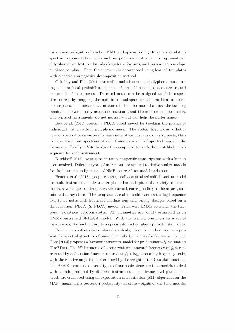
The distribution of the note sequences P (N) is modelled in a Dynamic
Bayesian Network with two layers of hidden nodes: a chord layer and a note
activity layer, as shown in Figure 2.6. The symbolic model makes use of a chord
model and 5 sub-models for temporal dependencies of notes and chords and
harmonic dependencies between notes. Knowledge about chord progressions
is modelled in the chord model, and relations between chords and pitches are
modelled in a harmony sub-model. Each of the other 4 sub-models deals with
a di↵erent property of pitch, for note duration, melodic intervals in voices, the
degree of polyphony per frame and neighbouring pitches, respectively. In or-
der to e↵ectively deal with the high dimensionality of the distributions, the note
combination distribution is factorised into a product of single note distributions.
Sub-models are normalised and combined by means of linear or log-linear inter-
polation for each note distribution. The proposed symbolic model is evaluated
on symbolic data and on audio data. The second evaluation is in combination
with an NMF-based acoustic model [Raczynski et al., 2007]. In both experi-
ments the proposed model outperforms the baseline Bernoulli model.
Sigtia et al. [2014] use a Music Language Model (MLM) to improve au-
tomatic music transcription performance. The MLM is based on Recurrent
Neural Networks (RNNs), which can model long-term temporal dependencies,
36
C1 C2 . . . Ct . . . CT
N1 N2 . . . Nt . . . NT
S1 S2 St ST
Figure 2.6: Dynamic Bayesian Network structure with three layers of variables:the hidden chords Ct and note combinations Nt, and observed salience St
and the acoustic AMT model is based on probabilistic latent component anal-
ysis (PLCA) [Benetos et al., 2013a]. First, the pre-trained MLM generates
a prediction based on the results of the PLCA-based acoustic model (a pitch
activation distribution). Then, the prediction is combined with the pitch acti-
vation distribution via a Dirichlet prior. Finally the combined pitch activation
is weighted and added to the output of the acoustic model. With the RNN
trained on symbolic music data from the Nottingham dataset,4 the proposed
hybrid models outperform the baseline acoustic AMT system by 3 percentage
points in terms of note-wise F-measure on the Bach10 dataset [Duan et al.,
2010] of multiple-instrument polyphonic music.
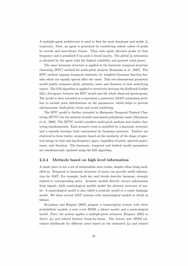
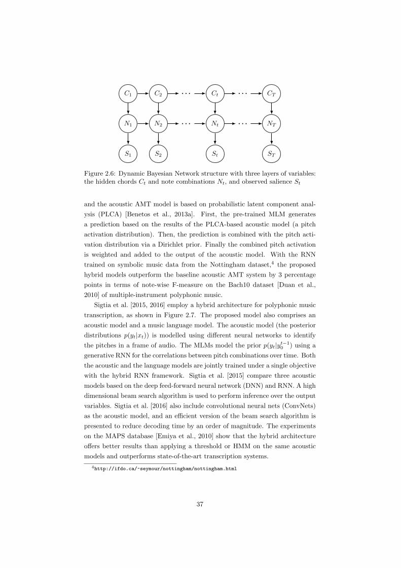
Sigtia et al. [2015, 2016] employ a hybrid architecture for polyphonic music
transcription, as shown in Figure 2.7. The proposed model also comprises an
acoustic model and a music language model. The acoustic model (the posterior
distributions p(yt|xt)) is modelled using di↵erent neural networks to identify
the pitches in a frame of audio. The MLMs model the prior p(yt|yt�10 ) using a
generative RNN for the correlations between pitch combinations over time. Both
the acoustic and the language models are jointly trained under a single objective
with the hybrid RNN framework. Sigtia et al. [2015] compare three acoustic
models based on the deep feed-forward neural network (DNN) and RNN. A high
dimensional beam search algorithm is used to perform inference over the output
variables. Sigtia et al. [2016] also include convolutional neural nets (ConvNets)
as the acoustic model, and an e�cient version of the beam search algorithm is
presented to reduce decoding time by an order of magnitude. The experiments
on the MAPS database [Emiya et al., 2010] show that the hybrid architecture
o↵ers better results than applying a threshold or HMM on the same acoustic
models and outperforms state-of-the-art transcription systems.
4http://ifdo.ca/
~
seymour/nottingham/nottingham.html
37
y1 y2 y3 y4 . . .
x1 x2 x3 x4
Figure 2.7: The hybrid architecture of the AMT systems in [Sigtia et al., 2015,2016].
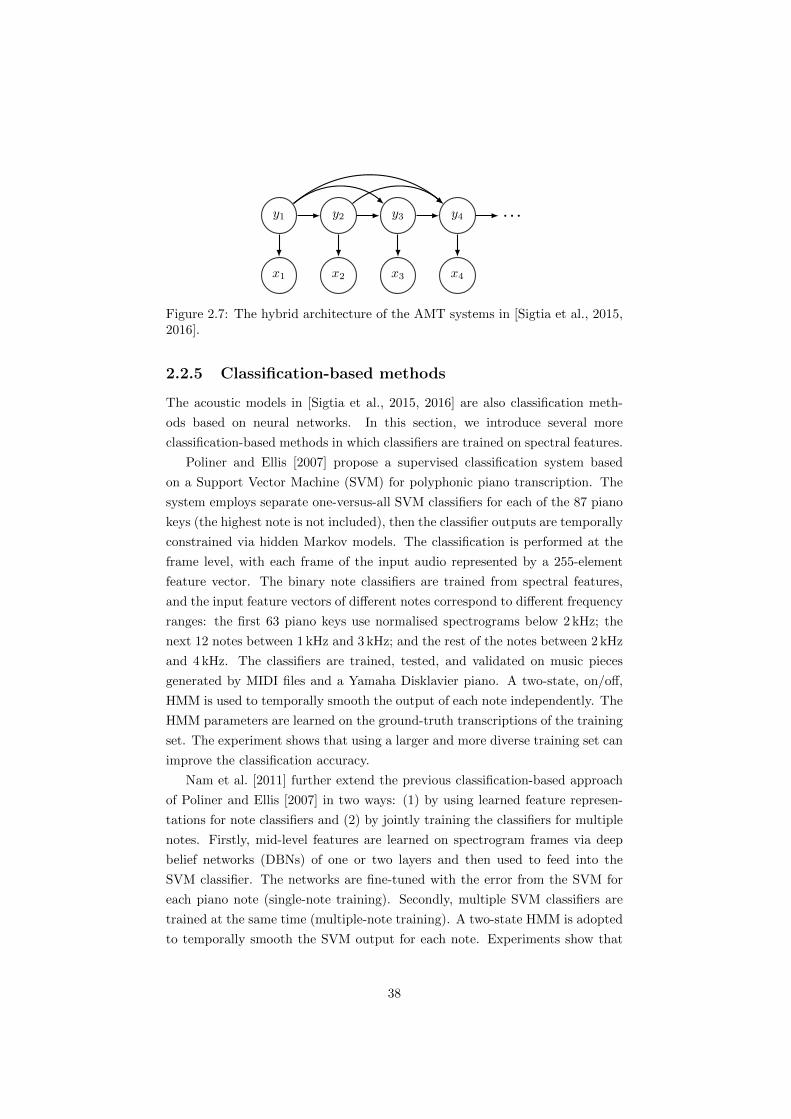
2.2.5 Classification-based methods
The acoustic models in [Sigtia et al., 2015, 2016] are also classification meth-
ods based on neural networks. In this section, we introduce several more
classification-based methods in which classifiers are trained on spectral features.
Poliner and Ellis [2007] propose a supervised classification system based
on a Support Vector Machine (SVM) for polyphonic piano transcription. The
system employs separate one-versus-all SVM classifiers for each of the 87 piano
keys (the highest note is not included), then the classifier outputs are temporally
constrained via hidden Markov models. The classification is performed at the
frame level, with each frame of the input audio represented by a 255-element
feature vector. The binary note classifiers are trained from spectral features,
and the input feature vectors of di↵erent notes correspond to di↵erent frequency
ranges: the first 63 piano keys use normalised spectrograms below 2 kHz; the
next 12 notes between 1 kHz and 3 kHz; and the rest of the notes between 2 kHz
and 4 kHz. The classifiers are trained, tested, and validated on music pieces
generated by MIDI files and a Yamaha Disklavier piano. A two-state, on/o↵,
HMM is used to temporally smooth the output of each note independently. The
HMM parameters are learned on the ground-truth transcriptions of the training
set. The experiment shows that using a larger and more diverse training set can
improve the classification accuracy.
Nam et al. [2011] further extend the previous classification-based approach
of Poliner and Ellis [2007] in two ways: (1) by using learned feature represen-
tations for note classifiers and (2) by jointly training the classifiers for multiple
notes. Firstly, mid-level features are learned on spectrogram frames via deep
belief networks (DBNs) of one or two layers and then used to feed into the
SVM classifier. The networks are fine-tuned with the error from the SVM for
each piano note (single-note training). Secondly, multiple SVM classifiers are
trained at the same time (multiple-note training). A two-state HMM is adopted
to temporally smooth the SVM output for each note. Experiments show that
38

better transcription results can be achieved by using the learned feature from a
DBN, especially the one-layer DBN, in comparison to the normalised spectro-
gram used by Poliner and Ellis [2007]. Multiple-note training improves training
speed and classification performance in comparison to single-note training. The
classification approach outperforms compared piano transcription methods.
Bock and Schedl [2012] propose a method to simultaneously detect onsets
and pitches of piano notes based on a recurrent neural network. The compressed
input of the neural network is obtained by filtering two magnitude spectrograms
of di↵erent window lengths with semitone filter-banks. The system is built on
a Bidirectional Recurrent Neural Network (BRNN) which models both the past
and future context of the notes. A Long Short-Term Memory (LSTM) unit is
used to ensure that the BRNN only use input values inside the memory cell.
The system has three bidirectional hidden layers with 88 LSTM units each. The
regression output layer has 88 units for all piano pitches. Onsets of each pitch
are detected by applying a standard local maximum peak picking algorithm on
the smoothed neural network output. Solo piano music pieces from di↵erent
piano datasets are used for training and testing. Evaluation indicates that the
reduction on note detection errors is mainly related to the single regression
output layer which detects piano notes simultaneously.
2.2.6 Note tracking
Automatic music transcription methods usually work in two steps. In the first
step, the music piece is segmented into frames of equal intervals, and pitches
are estimated in each frame. In the second step, estimated pitches of adjacent
frames are grouped together to form note events, then hence onsets and o↵sets.
There are also note-level systems which directly model the discrete note events.
In the following, we first introduce some basic methods for converting frame-wise
results into note events, then we illustrate several note-level systems.
Thresholding
For some methods, for example matrix-factorisation-based methods, a threshold
is applied to obtain a binary output [Wang et al., 2008, 2009, Grindlay and Ellis,
2011]. The threshold is usually adapted to the maximum value of each piece
[Vincent et al., 2010, O’Hanlon and Plumbley, 2013]:
Thre = �maxk,t
Hak,t. (2.14)
the optimal value for parameter � is usually determined by training.
39
Tavares et al. [2016] provide an unsupervised way to choose the threshold
for NMF-based piano transcription. Ideally for an activation matrix, its values
are sparse with only a few notes active at any given time, and high activation
values are related to true positives. The system assumes that the envelope of a
histogram of the activation matrix has the rough shape of a reverse sigmoid. In
order to find the elbow of the envelope, the method uses 10 threshold candidates
equally located between the maximum and minimum values in the activation
matrix (from 0 to 1 for normalised activations). For each piece, the candidate
with least second di↵erential is found as the elbow:
ie = argmini[(thi+1
� thi)� (thi� thi�1)], (2.15)
where thi indicates the number of active pitches using the ith threshold candi-
date. While using the elbow value as a threshold leads to a low mean F-measure
with high Recall and low Precision rates, then the optimal threshold is adjusted
to ie+0.3 with tests on three datasets. In the experiments, the method provides
better results than using a threshold trained on a di↵erent dataset.
Minimum-duration pruning
After thresholding, notes are detected in the time-pitch representation by con-
verting pitches found in consecutive frames into notes. There are some short
false-alarm notes brought by fluctuations of the activations. Minimum duration
pruning is applied to remove those short notes that fail to reach a duration
threshold [Dessein et al., 2010].
HMM smoothing
Hidden Markov models (HMMs) [Rabiner, 1989] are frequently employed to
provide a smooth output at the post-processing step. In order to decrease the
search space, HMMs are usually applied in a pitch-wise fashion, either using
two states per pitch to detect that a note is active or not [Poliner and Ellis,
2007, Benetos and Dixon, 2012a], or using states corresponding to several stages
of a note (attack, decay, sustain and release) which follow a certain sequence
[Ryynanen and Klapuri, 2005, Cheng et al., 2015b]. Pitch-wise HMM parame-
ters (state transitions and priors) are learned on symbolic representations, such
as a ground-truth training set or MIDI files, while the observation probability is
set based on the frame-wise transcribed results. The most likely state sequence
is estimated using the Viterbi algorithm.
40
Note-level methods
Several note-level systems are built with temporal evolution modelling. The
HTC [Kameoka et al., 2007] and HTTC [Miyamoto et al., 2008] methods model
the observed power envelope of a single source by weighted Gaussian function
kernels. Chen et al. [2012]’s preliminary work uses an exponential model for en-
ergy evolution of notes. Berg-Kirkpatrick et al. [2014] represent the energy evo-
lution of a piano note by a trained envelope. Ewert et al. [2015] represent both
time-varying timbre and temporal evolution of piano notes by time-frequency
patches. In these systems, a note event is represented by a single amplitude
parameter for its whole duration with the modelled temporal evolution, which
provides promising transcription results. In addition, Cogliati and Duan [2015]
propose a note level system informed by detected onsets, which also approxi-
mates decays of piano partials with a sum of two decaying exponentials. The
HTC and HTTC methods have been already described in Section 2.2.3. We will
introduce the other four systems in detail as follows.
Chen et al. [2012] extend the hierarchical eigeninstrument model of Grind-
lay and Ellis [2011] for multi-instrument music transcription using note-level
templates. In this method, musical notes are assumed to consist of a relatively
invariant attack, and a decay that depends on the overall duration of the note.
In order to represent notes with various durations for each pitch of di↵erent
sources, the system applies a parametric transformation step, controlling the
spectral evolution and amplitude envelope. In the parametric form, a non-
linear time warp is used to match notes of varying durations and to describe
the nonuniformity across attack and decay. In addition, the overall amplitude
decay is formulated by an exponential decay function. The method provides
a significant improvement compared to a frame-level system, with better note-
level transcription results on real woodwind excerpts and piano music pieces.
Berg-Kirkpatrick et al. [2014] present a probabilistic model comprising dis-
crete musical events. The generative system is built on three models. For each
pitch, there are (1) an event model, including discrete note events having a
velocity and duration, (2) an activation model, generated based on the event
model and an envelope parameter, and (3) a spectrogram model, generated by
the activations and spectral parameters of the pitch. The observed spectrogram
is reconstructed by adding the component spectrograms of all pitches. A block-
coordinate ascent procedure is performed to estimate the unknown parameters.
The spectral and envelope parameters are learned on isolated, synthesised, pi-
ano sounds. The event parameters are learned by counting note occurrences in
numerous symbolic music data. The pre-learned parameters are updated dur-
ing the decoding to predict transcriptions with fitted parameters. The approach
41
outperforms state-of-the-art methods on piano music transcription, especially
on onset-wise metrics.
Ewert et al. [2015] present a novel transcription method based on non-
negative matrix deconvolution with the variable note lengths modelled by a
dynamic system. The system assumes that recordings of individual notes of
played instruments are available, and uses the spectrogram of the whole note
as a time-frequency patch. Frames in a patch are identified with states in a
dynamic system. The system performs transcription by operating the following
two steps iteratively. First, the best fitting state sequence is tracked pitch by
pitch using dynamic programming to form notes with various lengths. Then
note objects of all pitches are updated jointly in a global optimisation, with
frames of each note object sharing the same activation parameter. The joint
estimation helps to avoid degenerate local minima caused by parameter decou-
pling in the first step. The system is tested on 10 MIDI files from a piano
playing competition.5 Both the test dataset and training dataset (individual
piano notes) are generated by Native Instruments Vienna Concert Grand VST
plugin using MIDI files. The note-wise onset F-measure achieves as high as 88%
in the experiment.
Cogliati and Duan [2015] propose a note-level spectrogram factorisation
method exploiting the temporal evolution of piano notes. The method detects
note onsets from the audio spectral flux using an artificial neural network. The
audio signal is segmented by the detected onsets. In each segment, partials of
notes lasting from the previous segment are set to zeros; only partials of notes
starting at the current segment are processed by a greedy search algorithm.
Notes are successively added with the lowest cost. An additional note is valid
only if the cost function decreases by more than 5%; otherwise the search stops.
During dictionary learning, a sum of two decaying exponentials is used to ap-
proximate the amplitude evolution of active partials. Frequency bins fitting this
parametric evolution are retained; and noisy bins are set to zeros. In addition,
a new cost function is proposed for spectrogram similarity. The cost function
weights the reconstruction error according to the energy present in the original
spectrogram, which works better than the L1-norm, L2-norm and KL-divergence
in the experiments.
2.3 Techniques for NMF-based AMT systems
In this section, we review techniques applied to non-negative matrix factorisa-
tion for automatic music transcription (AMT). First we present a general frame-
5http://www.piano-e-competition.com
42

work for AMT systems based on NMF in Section 2.3.1, including front-end,
post-processing of standard AMT systems, and parameter estimation methods
in the NMF framework. Then in Section 2.3.2 we specify constraints used to im-
pose sparsity, smoothness and harmonicity/inharmonicity, which lead to more
meaningful decompositions. In Section 2.3.3, we introduce the Bayesian exten-
sion of NMF, and show ways of using prior information to enforce constraints,
especially methods which impose temporal continuity on activations.
2.3.1 A general framework for NMF-based AMT
An AMT system starts from an audio signal and ends with a symbolic represen-
tation, in the form of a time-pitch representation. NMF is the key part of the
system, which works on the time-frequency representation matrix of the signal,
and provides an activation matrix as a mid-level representation of the sym-
bolic output. The general framework of an NMF-based AMT system consists of
three main parts: the front-end providing the time-frequency representation of
the signal, the NMF model for estimating unknown parameters, and the post-
processing step with a binary output, as shown in Figure 2.8. We will describe
each part individually in the following sections.
Time-frequency representation
The front-end of an NMF-based transcription system produces a non-negative
time-frequency (TF) representation of the signal. NMF decomposes the TF
representation into a linear combination of spectral bases with non-negative
constraints. The transform F to produce the TF representation should also
exhibit linearity, that is F(ax + by) = aF(x) + bF(y), or at least F(ax +
by) ⇡ aF(x)+ bF(y). Among various transform methods, we focus on three TF
representations as follows.
Short-Time Fourier Transform (STFT)
The Short-Time Fourier Transform (STFT) is a common TF representation with
a linear frequency scale. As reviewed by Bay et al. [2009], most AMT systems
employ STFT as a front-end. To obtain a spectrogram by STFT, the signal is
segmented into overlapping frames by a window function. The discrete Fourier
transform is performed on each frame to get the short-time spectrum.
This method is a fundamental transform method with many available im-
plementations. The frequency bins are linearly spaced, giving an intuitive TF
image. AMT systems usually work on the magnitude spectrogram or power
spectrogram. Only a few papers use the complex spectrogram with complex
NMF [Kameoka et al., 2009, Kirchho↵ et al., 2014].
43
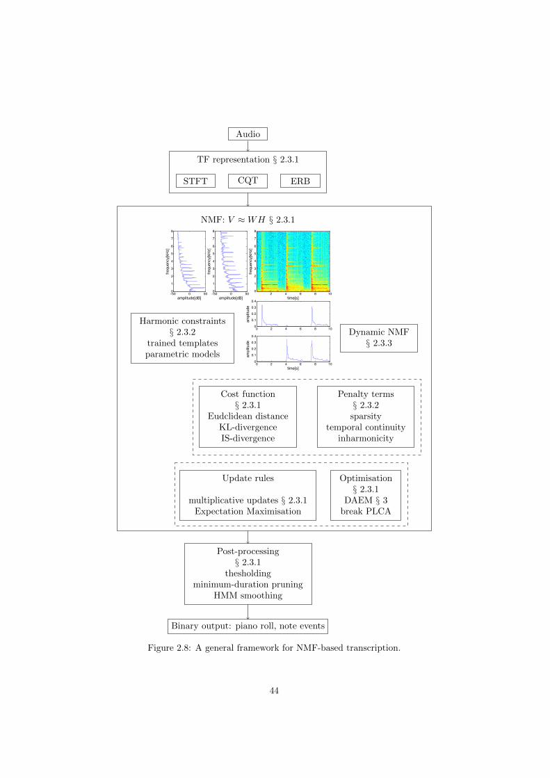
Audio
TF representation § 2.3.1
CQTSTFT ERB
NMF: V ⇡WH § 2.3.1
0
1
2
3
4
5
6
7
8
−50 0 50
frequency[kHz]
amplitude[dB]0
1
2
3
4
5
6
7
8
−50 0 50
frequency[kHz]
amplitude[dB]
frequency[kHz]
time[s]2 4 6 8 10
0
1
2
3
4
5
6
7
8
0 2 4 6 8 100
0.1
0.2
0.3
0.4
amplitude
0 2 4 6 8 100
0.1
0.2
0.3
0.4
amplitude
time[s]
Dynamic NMF§ 2.3.3
Harmonic constraints§ 2.3.2
trained templatesparametric models
Cost function§ 2.3.1
Eudclidean distanceKL-divergenceIS-divergence
Penalty terms§ 2.3.2sparsity
temporal continuityinharmonicity
Update rules
multiplicative updates § 2.3.1Expectation Maximisation
Optimisation§ 2.3.1
DAEM § 3break PLCA
Post-processing§ 2.3.1
thesholdingminimum-duration pruning
HMM smoothing
Binary output: piano roll, note events
Figure 2.8: A general framework for NMF-based transcription.
44

Constant-Q Transform (CQT)
Constant-Q transform (CQT) provides a TF representation on a log-frequency
scale. The Q in CQT indicates the quality factor, defined as [Brown, 1991]:
Q = fk/�fk, (2.16)
where fk and �fk are the central frequency and the frequency resolution of the
kth bin, respectively. Then the window length of the kth bin is given by
N [k] =fs�fk
= (fsfk
)Q, (2.17)
where fs is the sampling rate. In the constant-Q transform, the central frequen-
cies of the frequency bins are geometrically spaced and the Q value is constant.
The geometrically spaced frequency bins are in line with the musical scale, be-
cause the fundamental frequencies (f0s) of musical pitches are equally spaced
in the log frequency scale. Constant Q means that the window sizes of the fre-
quency bins are inversely proportional to their centre frequencies. This results
in varying time and frequency resolutions along the frequency axis, with better
frequency resolution at low frequencies and better time resolution at high fre-
quencies. This frequency scale is closer to human auditory perception than the
STFT [Schorkhuber and Klapuri, 2010].
Because of the geometrically spaced frequency bins in the CQT, the intervals
between f0s and harmonics are constant for all pitches, which allows the note
spectra to be shiftable along the log-frequency axis. However, simply shifting a
spectrum for all pitches is not practical for AMT, because the spectra of di↵erent
pitches usually have di↵erent harmonic distributions. This shift-invariant char-
acteristic has been used successfully to shift templates among a small frequency
range [Benetos and Dixon, 2012a].
Some e�cient implementations of CQT can be found in [Schorkhuber and
Klapuri, 2010, Fillon and Prado, 2012, Schorkhuber et al., 2014].
Equivalent Rectangular Bandwidth-scale (ERB-scale) TF representa-
tion
The ERB-scale TF representation is an auditory-motivated TF representation,
with the ERB scale defined by [Moore and Glasberg, 1996]
fERB = 9.26 log(0.00437fHz + 1). (2.18)
As applied in musical source separation [Vincent, 2006, Duong et al., 2010] and
automatic music transcription [Vincent et al., 2008, Bertin et al., 2009a, 2010,
45
Vincent et al., 2010], the ERB-scale TF representation is computed as follows.
The signal x(t) is passed through a bank of filters Hf (t), providing subband
signals xf (t) of the f th filter:
xf (t) =X
⌧
Hf (t)x(t� ⌧). (2.19)
The centre frequencies of the filters are linearly spaced on the ERB scale. The
distribution of the filters is approximately linear in the low frequency range
(below 500 Hz), and approximately constant-Q at high frequencies (above 2000
Hz) [Necciari et al., 2013]. The main-lobe bandwidth of each filter is set to four
times the frequency di↵erence between the centre frequencies of adjacent filters.
The magnitude frequency response Gf of the f th filter can then be analytically
computed as a combination of sine cardinal (sinc) functions.
It is shown that in comparison to the STFT, the ERB scale provides a
representation of better temporal resolution in the higher frequency range with
smaller size [Vincent et al., 2008]. In addition, tests on AMT show that better or
at least similar performance can be achieved at lower computational cost using
the ERB-scale representation [Vincent et al., 2008, O’Hanlon and Plumbley,
2013, Benetos and Weyde, 2015b].
‘The ERBlet transform’, an alternative implementation of an invertible
ERB-scale representation, is available in [Necciari et al., 2013].
Non-negative matrix factorisation
After obtaining the TF representation, for example the spectrogram, the tran-
scription systems employ NMF to represent the spectrogram V as a linear com-
bination of spectral bases W:
Vft ⇡
RX
r=1
WfrHrt, (2.20)
where V 2 RF⇥T , W 2 RF⇥R and H 2 RR⇥T are non-negative matrices, and
f , t and r are indices of the frequency bin, time frame and latent component,
respectively. R is chosen in order to perform a low-rank matrix approximation
(R(F + T )⌧ FT ).
Cost functions
We denote V = WH as the reconstruction. NMF estimates W and H by min-
imising the distance between V and V. This distance is called the cost function
or the objective function [Lee and Seung, 1999], which is initially represented
46
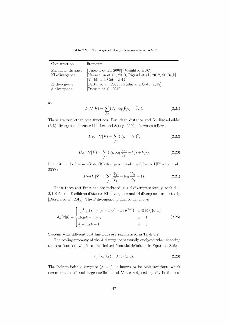
Table 2.2: The usage of the �-divergences in AMT
Cost function literature
Euclidean distance [Vincent et al., 2008] (Weighted EUC)KL-divergence [Hennequin et al., 2010, Rigaud et al., 2012, 2013a,b]
[Yoshii and Goto, 2012]IS-divergence [Bertin et al., 2009b, Yoshii and Goto, 2012]�-divergence [Dessein et al., 2010]
as:
D(V|V) =X
f,t
(Vft log(Vft)� Vft). (2.21)
There are two other cost functions, Euclidean distance and Kullback-Leibler
(KL) divergence, discussed in [Lee and Seung, 2000], shown as follows,
DEuc(V|V) =X
f,t
(Vft � Vft)2, (2.22)
DKL(V|V) =X
f,t
(Vft logVft
Vft
� Vft + Vft). (2.23)
In addition, the Itakura-Saito (IS) divergence is also widely-used [Fevotte et al.,
2009]:
DIS (V|V) =X
f,t
(Vft
Vft
� logVft
Vft
� 1). (2.24)
These three cost functions are included in a �-divergence family, with � =
2, 1, 0 for the Euclidean distance, KL divergence and IS divergence, respectively
[Dessein et al., 2010]. The �-divergence is defined as follows:
d�(x|y) =
8>>><
>>>:
1�(��1) (x
� + (� � 1)y� � �xy��1) � 2 R \ {0, 1}
xlogxy � x+ y � = 1
xy � logx
y � 1 � = 0
(2.25)
Systems with di↵erent cost functions are summarised in Table 2.2.
The scaling property of the �-divergence is usually analysed when choosing
the cost function, which can be derived from the definition in Equation 2.25:
d�(�x|�y) = ��d�(x|y). (2.26)
The Itakura-Saito divergence (� = 0) is known to be scale-invariant, which
means that small and large coe�cients of V are weighted equally in the cost
47

function [Fevotte et al., 2009]. When � > 0, more emphasis is put on the
frequency components of higher energy, and the emphasis increases with �.
When � < 0, the e↵ect is the converse [Dessein et al., 2010].
We apply a simple test of di↵erent � 2 {2, 1, 0} using an isolated piano
tone from the ‘ENSTDkCl’ subset of the MAPS database [Emiya et al., 2010].
The piano tone with the fundamental frequency of 440Hz (MIDI index 69) is
produced by a Disklavier piano. The waveform and spectrogram (normalised
to a maximum of 1) of the signal are shown in Figure 2.9. A rank-one NMF
is performed on the amplitude spectrogram with di↵erent � 2 {2, 1, 0}, and
the maximum of the activation is normalised to 1. The spectral basis is also
normalised to a maximum of 1 after the iterations for an intuitive comparison.
The results are illustrated in Figure 2.10, which are basically in line with the
analysis in previous literature. The activation of � = 2 resembles more the
envelope of the partial with largest energy, as shown in the fundamental fre-
quency amplitude in the spectrogram of Figure 2.9. By contrast, the activation
of � = 0 is equally sensitive to energy changes of all frequencies, therefore the
trajectory fluctuates. The activation of � = 1 is somewhere in between. It
smoothly represents the decaying energy of the signal.
Update rules
There are several ways to estimate parameters in NMF. Here we employ mul-
tiplicative update rules for parameter estimation. The rules can be obtained
by choosing an adaptive step in gradient descent [Lee and Seung, 2000]. The
derivative of the cost function D with respect to (w.r.t) ✓, r✓D(✓), is written
as a di↵erence of two non-negative functions:
r✓D(✓) = r+✓ D(✓)�r�
✓ D(✓), (2.27)
where r+✓ D(✓) and r�
✓ D(✓) are the absolute values of the positive and negative
parts of the derivative, respectively. The multiplicative algorithm is given by:
✓ ✓.r
�✓ D(✓)
r
+✓ D(✓)
. (2.28)
For the �-divergence, the derivative is derived as:
r✓D(✓) = (V ��1� V V ��2)r✓V . (2.29)
48
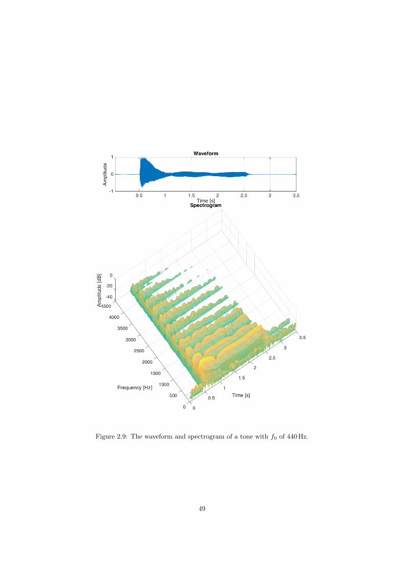
Figure 2.9: The waveform and spectrogram of a tone with f0 of 440Hz.
49

0 2000 4000 6000 8000Frequency [Hz]
-50
-40
-30
-20
-10
0
Am
plit
ude [dB
]
Normalised spectral basis
0.5 1 1.5 2 2.5 3 3.5Time [s]
-40
-30
-20
-10
0
Am
plit
ude [dB
]
Normalised activation
(a) (� = 2)
0 2000 4000 6000 8000Frequency [Hz]
-50
-40
-30
-20
-10
0
Am
plit
ude [dB
]
Normalised spectral basis
0.5 1 1.5 2 2.5 3 3.5Time [s]
-40
-30
-20
-10
0
Am
plit
ude [dB
]
Normalised activation
(b) (� = 1)
0 2000 4000 6000 8000Frequency [Hz]
-50
-40
-30
-20
-10
0
Am
plit
ude [dB
]
Normalised spectral basis
0.5 1 1.5 2 2.5 3 3.5Time [s]
-40
-30
-20
-10
0
Am
plit
ude [dB
]
Normalised activation
(c) (� = 0)
Figure 2.10: Spectral bases and activations obtained using di↵erent cost func-tions.
50
Then the updates for W and H with �-divergence are as follows [Fevotte, 2011],
H H.WT [(WH).(��2).V ]
WT [WH].(��1), (2.30)
W W.[(WH).(��2).V ]HT
[WH].(��1)HT. (2.31)
The update rules are iterated alternately until convergence.
Optimisation
Parameter estimation is achieved by finding the minimum of the cost function.
Optimisation methods can help to find the global minimum or at least a bet-
ter local minimum when the problem is non-convex. We will discuss the local
minimum problem of matrix-factorisation-based methods in Chapter 3, and in-
troduce an optimisation method to deal with this problem.
Post-processing
The activations indicate the volumes of di↵erent pitches. In order to provide a
binary output, we can simply apply a threshold on the activations. After that
minimum-duration pruning is commonly used to reduce erroneous notes with
short duration. To smooth the output, many systems apply Hidden Markov
Models to track the optimal state sequences. Readers are referred to Sec-
tion 2.2.6 for our summaries of these methods.
2.3.2 Constraints
The non-negative constraint allows NMF to provide part-based and meaningful
decompositions, but the result is not unique. It is related to the cost function,
estimation method, initialisation, scaling, constraints and so on. In this section,
we will discuss several commonly-used constraints. Besides non-negativity, spar-
sity and continuity are also proper assumptions for many real-world applications.
For music, another primary characteristic is the harmonic (or quasi-harmonic)
structure in the spectrum.
Bertin et al. [2010] summarise three ways to enforce constraints: adding
penalty terms to cost functions, using parametric models and choosing prior
distributions in the statistical Bayesian NMF. In this section, we review the
first two methods for constraints. We individually describe incorporating priors
in the Bayesian extension of NMF in Section 2.3.3.
51

Sparsity
Sparsity is the most common constraint for NMF, which can be enforced on
either decomposed matrix, depending on the specific application. We usually
assume the activation of each time frame is sparse in AMT.
Hoyer [2004] proposed to project the column of W or the row of H to achieve
a desired level of sparsity after each iteration. The sparsity is measured by the
relation between the L1 norm and the L2 norm:
g(x) =
p
n� ||x||1/||x||2p
n� 1, (2.32)
where Lp-norm is given by ||x||p := (Pn
i=1 |xi|p)1/p, and n is the dimension of
the vector x. The method is used for multiple pitch estimation with modified
sparsity measures [Cont, 2006, Cont et al., 2007].
An alternative method is to add a penalty term to the cost function [Eggert
and Korner, 2004], which is adapted from non-negative sparse coding [Hoyer,
2002]:
Cs(H) =X
r,t
g(Hrt),
C = D(V|WH) + �sCs(H), (2.33)
where g(x) = |x| is the L1-norm regularisation for measuring sparsity and �s
controls the degree of sparsity. Because all values are non-negative in NMF, the
L1-norm function can be expressed as g(x) = x. Note that the scaling problem
of choosing �s can be fixed by normalising Wr. Similarly, the L0-norm and L2-
norm are applied in [Peharz and Pernkopf, 2012] and [Smaragdis and Brown,
2003] for sparsity constraints, respectively.
In the equivalent probabilistic model (PLCA), the sparsity is enforced by
applying a power larger than 1 to the distribution [Benetos and Dixon, 2012a]:
Hrt H�srt . (2.34)
where �s is larger than 1. When we normalise the sum of the activations in
each frame to be 1, the activations in NMF can be seen as probabilities. So
the method in Equation 2.34 can also be applied in normalised NMF to enforce
sparsity.
Continuity
We review methods to enforce temporal continuity and spectral continuity on
the activations and spectral bases, respectively.
52

Temporal continuity
To enforce temporal continuity, Virtanen [2007] proposed to add a penalty on
the activations H to the cost function :
Ct(H) =RX
r=1
1
�2r
TX
t=2
(hr,t � hr,t�1)2. (2.35)
This constraint prevents a large change between activations in adjacent frames.
The standard deviation estimate �r =q
(1/T )PT
t=1 h2rt is used for normalisa-
tion, so the cost is not a↵ected by scaling. The IS divergence of amplitudes of
adjacent frames is also used as a penalty to impose temporal continuity, which
is also scale-invariant [Fevotte, 2011]. The cost function is written as:
C(W,H) = D(V|WH) + �tCt(H), (2.36)
where �t controls the degree of continuity.
Another temporal flatness term is proposed for temporal continuity, moti-
vated by spectral flatness [Becker et al., 2014]. The proposed term is presented
as:
Ct(H) =RX
r=1
1T
PTt=1 Hrt
T
qQTt=1 Hrt
. (2.37)
Spectral continuity
Two spectral terms are employed to enforce spectral continuity to penalise large
spectral variations [Becker et al., 2014], which take the same forms as the pre-
vious temporal terms. One is the spectral-wise squared di↵erence motivated
by the temporal squared di↵erence, Equation 2.35. The other penalty is the
inverted spectral flatness descriptor, written as:
Csp(W) =RX
r=1
1F
PFf=1 Wfr
F
qQFf=1 Wfr
. (2.38)
This penalty term is also added to the cost function:
C(W,H) = D(V|WH) + �spCsp(W), (2.39)
where �sp controls the degree of spectral continuity.
53

Harmonic constraints
A pitched sound generates frequency components at or near the multiples of
its fundamental frequency, i.e. the harmonics or partials, with a comb-shaped
spectrum. In NMF-based systems, the harmonic structure is constrained by each
spectral basis wr. In this section, we show several ways to enforce harmonicity
or inharmonicity.
Training templates
The harmonic structure of a pitch can be obtained by template training. A
template is an average of the spectral distribution over the duration of the note,
which is usually learned on an isolated note. When we have access to sound
samples of the sources, we can train the templates first and then keep them
fixed to perform supervised NMF, or semi-automatic transcription [Kirchho↵,
2013].
The previously-trained templates can be adapted to the test data. Benetos
et al. [2014] proposed a template adaptation system to match the test dataset.
The system first transcribes the test music pieces with trained templates. Then
activations of high values are fixed, and corresponding templates are updated
using the test data. Finally music pieces are transcribed again with the adapted
templates.
Parametric models
The harmonic structure can be parameterised as a harmonic comb, with peaks
at harmonic positions. The spectral basis is given as:
Wfr =X
k
akrg(f � fkr), (2.40)
where Wfr is the value of spectral basis r in the f th frequency bin. k is the index
of the partial. fkr and akr are the frequency and amplitude of the kth partial
of the rth spectral basis, respectively. g(f) represents the frequency response of
the window function. The frequency response covers the whole frequency range,
but usually only a certain range is used, such as the main lobe of the hamming
window [Rigaud et al., 2012, 2013a,b].
This parametric harmonic comb has been employed in music transcription
[Vincent et al., 2008, Hennequin et al., 2010, Yoshii and Goto, 2012, Rigaud
et al., 2013b], music source separation [Hennequin et al., 2011b] and piano sound
analysis [Rigaud et al., 2012, 2013a]. The harmonicity or inharmonicity of the
music sounds is enforced by the relation between f0r and fkr. Usually three
54
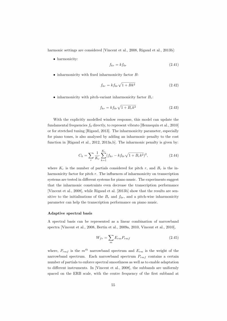
harmonic settings are considered [Vincent et al., 2008, Rigaud et al., 2013b]:
• harmonicity:
fkr = kf0r (2.41)
• inharmonicity with fixed inharmonicity factor B:
fkr = kf0rp
1 +Bk2 (2.42)
• inharmonicity with pitch-variant inharmonicity factor Br:
fkr = kf0rp
1 +Brk2 (2.43)
With the explicitly modelled window response, this model can update the
fundamental frequencies f0 directly, to represent vibrato [Hennequin et al., 2010]
or for stretched tuning [Rigaud, 2013]. The inharmonicity parameter, especially
for piano tones, is also analysed by adding an inharmonic penalty to the cost
function in [Rigaud et al., 2012, 2013a,b]. The inharmonic penalty is given by:
Ch =X
r
1
Kr
KrX
k=1
(fkr � kf0rp
1 +Brk2)2, (2.44)
where Kr is the number of partials considered for pitch r, and Br is the in-
harmonicity factor for pitch r. The influences of inharmonicity on transcription
systems are tested in di↵erent systems for piano music. The experiments suggest
that the inharmonic constraints even decrease the transcription performance
[Vincent et al., 2008], while Rigaud et al. [2013b] show that the results are sen-
sitive to the initialisations of the Br and f0r, and a pitch-wise inharmonicity
parameter can help the transcription performance on piano music.
Adaptive spectral basis
A spectral basis can be represented as a linear combination of narrowband
spectra [Vincent et al., 2008, Bertin et al., 2009a, 2010, Vincent et al., 2010],
Wfr =X
m
ErmPrmf (2.45)
where, Prmf is the mth narrowband spectrum and Erm is the weight of the
narrowband spectrum. Each narrowband spectrum Prmf contains a certain
number of partials to enforce spectral smoothness as well as to enable adaptation
to di↵erent instruments. In [Vincent et al., 2008], the subbands are uniformly
spaced on the ERB scale, with the centre frequency of the first subband at
55

the fundamental frequency fr1 and subsequent subbands linearly spaced, for
example by 3 ERB. The subband spectral shape is defined as the symmetric
approximation of the response of the gammatone filter of the corresponding
bandwidth.
In comparison to the weighted sum of each partial, the number of free pa-
rameters of this model is reduced. It keeps the harmonic structure and flexibility
to adapt to various instruments, and also helps to enforce spectral smoothness.
2.3.3 Bayesian extension of NMF
In previous sections we illustrate how NMF works with penalty terms and deter-
ministic constraints. In this section we introduce a Bayesian extension of NMF,
which interprets NMF from a statistical perspective and o↵ers a principled way
to incorporate prior knowledge.
Initially in NMF, Lee and Seung explained the cost function
D(V|WH) =X
f,t
(Vft log(WH)ft � (WH)ft) (2.46)
as a generative model, in which Vft is generated by adding Poisson noise to
the product (WH)ft [Lee and Seung, 1999]. The cost function is related to the
likelihood of generatingV from basesW and activationsH. The correspondence
between the cost functions and probabilistic generative models is analysed in
[Abdallah and Plumbley, 2004, Virtanen et al., 2008, Cemgil, 2009, Schachtner
et al., 2014, Smaragdis et al., 2014], which is given by
� log p(V|WH) = aD(V|WH) + b, (2.47)
where a and b are constants with respect to WH, and a > 0. This means
that minimising the cost function D(V|WH) is equivalent to maximising the
log likelihood log p(V|WH). We adapt a summary of the relation between the
cost functions and generative models from [Smaragdis et al., 2014] as shown in
Table 2.3. In AMT,V, V indicate the observed and reconstructed spectrograms,
respectively.
In the probabilistic model, parameters W and H can be estimated by the
maximum a posteriori (MAP) method.
(W,H) = argmaxW,H
log(P (W,H|V)). (2.48)
56
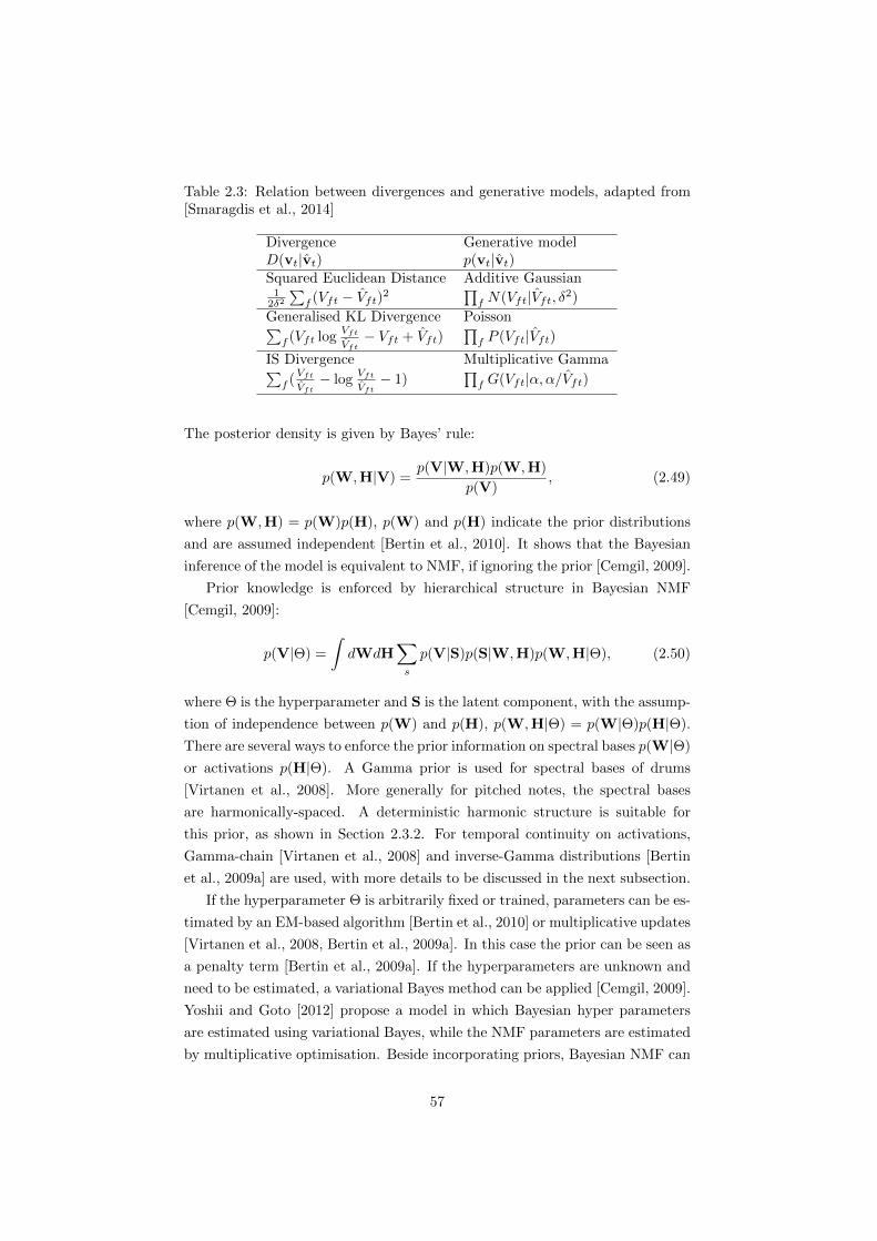
Table 2.3: Relation between divergences and generative models, adapted from[Smaragdis et al., 2014]
Divergence Generative modelD(vt|vt) p(vt|vt)Squared Euclidean Distance Additive Gaussian1
2�2P
f (Vft � Vft)2Q
f N(Vft|Vft, �2)
Generalised KL Divergence PoissonPf (Vft log
Vft
Vft� Vft + Vft)
Qf P (Vft|Vft)
IS Divergence Multiplicative GammaPf (
Vft
Vft� log Vft
Vft� 1)
Qf G(Vft|↵,↵/Vft)
The posterior density is given by Bayes’ rule:
p(W,H|V) =p(V|W,H)p(W,H)
p(V), (2.49)
where p(W,H) = p(W)p(H), p(W) and p(H) indicate the prior distributions
and are assumed independent [Bertin et al., 2010]. It shows that the Bayesian
inference of the model is equivalent to NMF, if ignoring the prior [Cemgil, 2009].
Prior knowledge is enforced by hierarchical structure in Bayesian NMF
[Cemgil, 2009]:
p(V|⇥) =
ZdWdH
X
s
p(V|S)p(S|W,H)p(W,H|⇥), (2.50)
where ⇥ is the hyperparameter and S is the latent component, with the assump-
tion of independence between p(W) and p(H), p(W,H|⇥) = p(W|⇥)p(H|⇥).
There are several ways to enforce the prior information on spectral bases p(W|⇥)
or activations p(H|⇥). A Gamma prior is used for spectral bases of drums
[Virtanen et al., 2008]. More generally for pitched notes, the spectral bases
are harmonically-spaced. A deterministic harmonic structure is suitable for
this prior, as shown in Section 2.3.2. For temporal continuity on activations,
Gamma-chain [Virtanen et al., 2008] and inverse-Gamma distributions [Bertin
et al., 2009a] are used, with more details to be discussed in the next subsection.
If the hyperparameter ⇥ is arbitrarily fixed or trained, parameters can be es-
timated by an EM-based algorithm [Bertin et al., 2010] or multiplicative updates
[Virtanen et al., 2008, Bertin et al., 2009a]. In this case the prior can be seen as
a penalty term [Bertin et al., 2009a]. If the hyperparameters are unknown and
need to be estimated, a variational Bayes method can be applied [Cemgil, 2009].
Yoshii and Goto [2012] propose a model in which Bayesian hyper parameters
are estimated using variational Bayes, while the NMF parameters are estimated
by multiplicative optimisation. Beside incorporating priors, Bayesian NMF can
57
employ statistical features of Bayesian models, such as non-parametric models
[Ho↵man et al., 2010, Yoshii and Goto, 2012].
Dynamic models
In basic NMF, the activations of di↵erent time frames are assumed independent.
Temporal continuity is achieved by post-processing the gains or by a constraint
in the cost function as shown in Section 2.3.2. In Bayesian NMF, temporal
continuity can be modelled by the prior for the activations. These models are
called dynamic models [Smaragdis et al., 2014], which are represented as:
ht ⇠ p(ht|ht�1, ✓), (2.51)
vt ⇠ p(vt|Wht), (2.52)
where ht is the activation vector at time frame t. The second equation repre-
sents a probabilistic view of the NMF model, with E[V|WH] = WH. The first
equation indicates that the activation of the current frame is related to previous
frames by a Markov model, where ✓ denotes the prior parameters. Gamma-chain
constraints are used for the activation continuity [Virtanen et al., 2008, Yoshii
and Goto, 2012], and an inverse-Gamma distribution is employed in [Bertin
et al., 2009a, 2010], defined as:
p(hrt|hrt�1) = IG(hrt|↵r, (↵r + 1)hrt�1), (2.53)
where IG is the inverse-Gamma distribution, and ↵r is arbitrarily fixed to con-
trol the degree of smoothness.
Other approaches apply Hidden Markov Models for temporal continuity
[Ozerov et al., 2009, Nakano et al., 2010, Mysore et al., 2010, Mohammadiha
et al., 2013]. With a probabilistic representation, the idea is formulated as:
qt ⇠ p(qt|qt�1), (2.54)
ht ⇠ p(ht|qt), (2.55)
where qt is the hidden state at time frame t. This model can use higher-level in-
formation with hidden states [Smaragdis et al., 2014]. Benetos and Dixon [2013]
use a probabilistic version (temporally-constrained PLCA) for multi-instrument
music transcription. The unknown parameters of the matrix factorisation meth-
ods and HMM are estimated jointly in this model.
58
2.4 Evaluation metrics
In order to evaluate the performance of the AMT methods, two levels of metrics
are commonly used, frame-level metrics (for multiple f0 estimation) and note-
level metrics (for note tracking). As transcription systems are now pursuing
higher-level representations, more systems are expected to include the instru-
ment information in the output. In this case, instrument-based evaluation is
also performed. We will introduce these three levels of metrics in the following.
They are also described in an annual evaluation campaign ‘Music Information
Retrieval Evaluation eXchange’ (MIREX) for Multiple Fundamental Frequency
Estimation & Tracking [MIREX, 2016].
2.4.1 Frame-level evaluation
For a frame-level evaluation, performance is evaluated frame by frame with an
interval of 10ms. If a detected f0 is in a range of ±3% of the ground truth
frequency, it is labelled as a correct detection. The overall accuracy (Acc) is
indicated using the definition in [Dixon, 2000]:
Acc =Ntp
Ntp +Nfp +Nfn(2.56)
where Ntp is the number of true positives, Nfp and Nfn are the numbers of false
positives and false negatives respectively. The frame-wise precision (P ), recall
(R) and F-measure (F ) are also used as accuracy metrics, defined in [Vincent
et al., 2010] as:
P =Ntp
Nsys, R =
Ntp
Nref, F =
2⇥R⇥ P
R+ P(2.57)
where Nsys = Ntp + Nfp denotes the number of detected pitches and Nref =
Ntp +Nfn is the number of ground-truth pitches.
Apart from the accuracy, the metrics below are defined for the frame-based
evaluation as well [Poliner and Ellis, 2007], including the rates of total errors
(Etot), substitution errors (Esubs), missed detections (Emiss) and false alarms
59

(Efa):
Esubs =
PTt=1 min(N t
ref , Ntsys)�N t
tpPTt=1 N
tref
(2.58)
Emiss =
PTt=1 max(0, N t
ref �N tsys)PT
t=1 Ntref
(2.59)
Efa =
PTt=1 max(0, N t
sys �N tref )PT
t=1 Ntref
(2.60)
Etot = Esubs + Emiss + Efa (2.61)
where t is the frame index and T is the total number of frames.
2.4.2 Note-level evaluation
To perform a note-level evaluation, the output is represented as a list of note
events, where each note event consists of an onset, an o↵set and a pitch. In the
MIREX public evaluations for Multiple Fundamental Frequency Estimation &
Tracking [MIREX, 2016], a note is considered correctly detected if the note is
within the following ranges of ground truth.
pitch range ±3%
onset range ± 50ms
o↵set range ± max {20% of the duration, 50ms }
The algorithms are evaluated in terms of onset-only and onset-o↵set using
the note-wise accuracy metrics, which are defined in a similar way to (2.56)
and (2.57). The onset-only precision, recall, F-measure and overall accuracy are
denoted as Pon , Ron , Fon and Accon , respectively. The onset-o↵set metrics are
Po↵ , Ro↵ , Fo↵ and Acco↵ .
2.4.3 Instrument-level evaluation
To evaluate a system at the instrument level, the output notes need to be labelled
with their corresponding instruments. Then, the performance for each instru-
ment can be measured using previous frame-wise and note-wise metrics. Con-
sidering that the contribution of each instrument is often monophonic, melody
extraction evaluation metrics are also used for this task [Bay et al., 2012]. The
evaluation metrics are calculated over all frames and all instruments, given as
60

Table 2.4: Public evaluation results on frame-wise accuracy (Accf ) and onset-only note-level F-measure Fon .
Year Baseline method Accf Fon
2011 [Yeh et al., 2010] 0.683 0.5602013 [Cheng et al., 2013] 0.620 0.5072014 [Duan et al., 2010] 0.553 0.4512014 [Bock and Schedl, 2012] - 0.5472014 [Dressler, 2011] 0.680 0.6592015 [Benetos and Weyde, 2015a] 0.654 0.6012016 [Benetos and Dixon, 2012a] 0.486 0.503
follows:
P =
Pi,t N
i,ttpcP
i,t Ni,ttp +N i,t
fp
(2.62)
R =
Pi,t N
i,ttpcP
i,t Ni,ttp +N i,t
fn
(2.63)
F =2⇥ P ⇥R
P +R(2.64)
Acc =
Pi,t N
i,ttpc +N i,t
tnPi,t N
i,ttp +N i,t
fp +N i,ttn +N i,t
fn
(2.65)
where Ntp , Ntn , Nfp and Nfn are the numbers of true positives, true negatives,
false positives and false negatives for pitched/unpitched detection, Ntpc denotes
the number of correct f0 in Ntp , and i and t are the instrument index and the
frame index, respectively.
2.4.4 Public evaluation
Some systems reviewed in this chapter have been submitted to the Music In-
formation Retrieval Evaluation eXchange (MIREX) for the task of Multiple
Fundamental Frequency Estimation & Tracking [MIREX, 2016]. We show the
results of the latest submissions based on the reviewed systems in Table 2.4.
The frame-wise accuracies Accf is evaluated on 40 test pieces and note-level
F-measures (onset-only) Fon is evaluated on 34 test pieces.
2.5 Conclusions
In this chapter, we first give a brief introduction to sound generation and per-
ception, by which we know that human perception of a musical tone is related
61
to its fundamental frequency, harmonics (partials) and spectrum. Then in Sec-
tion 2.1.2 we specify acoustical features of piano tones which are related to the
excitation mechanism and physical structure of the piano. We review AMT
systems according to the level of information employed by the system in Sec-
tion 2.2. First we introduce systems detecting a pitch using its period, harmon-
ics (partials) and spectrum, respectively. Then we review systems using high
level information, i.e. musicological models, for transcription, and also several
typical classification-based methods. At last, we present post-processing meth-
ods to generate note events and note-level systems which model discrete note
events directly. In Section 2.3, we present a general framework for NMF-based
transcription in detail, with commonly-used constraints. In Section 2.4 we sum-
marise commonly-used evaluation metrics of three levels (frame level, note level
and instrument level), and give a summary on public evaluation results.
In Chapter 3, we will address the local minimum problem of matrix de-
composition methods as indicated in Section 2.3.1. We work on an existing
transcription system based on the PLCA, the probabilistic counterpart of NMF,
with an optimisation method. Based on the theoretical analysis in Section 2.1.2,
we will study piano decay in Chapter 4, and model temporal evolution for piano
notes for transcription in Chapter 5 and Chapter 6.
62

Chapter 3
A Deterministic Annealing
EM Algorithm for AMT
In this chapter, we use a deterministic annealing EM (DAEM) algorithm to
deal with the local minimum problem of PLCA and show the improvement in
transcription performance by doing so. Matrix factorisation methods (such as
NMF and PLCA) are initialisation-sensitive and tend to converge to a local
minimum. There are several approaches to address this local minimum prob-
lem. Hofmann [1999] proposes a model based on a tempered EM algorithm to
avoid overfitting in probabilistic latent semantic analysis. Bertin et al. [2009b]
use the tempering scheme to favour the convergence of the Itakura-Saito (IS)
divergence to global minima. Experiments on music transcription show that
the IS-NMF can provide a good result by choosing a suitable temperature pa-
rameter. The deterministic annealing EM algorithm is proposed to optimise
the parameter estimation of EM-based methods [Ueda and Nakano, 1998]. It
has been used in a harmonic-temporal-structured clustering (HTC) model for
audio feature extraction [Kameoka et al., 2005], and to estimate the parameters
of Gaussian mixture models (GMMs) and hidden Markov models (HMMs) for
speaker and speech recognition [Itaya et al., 2005]. In the latter method DAEM
is shown to be e↵ective for GMM and HMM-based acoustic models. Smaragdis
and Raj [2007] state that using ‘annealing’ in PLCA helps to get ‘meaningful’
decompositions and quick convergence.
Here we focus on an existing PLCA-based transcription model [Benetos and
Dixon, 2012a], and apply the DAEM algorithm to tackle the local minimum
problem. In the proposed model, the PLCA update rules are modified by in-
troducing a ‘temperature’ parameter. At higher temperatures, general areas of
the search space containing good solutions are found. As the temperature is
63

gradually decreased, distinctions in the data are sharpened, resulting in a more
fine-grained optimisation at each successive temperature.
We describe transcription systems based on PLCA in Section 3.1. In Sec-
tion 3.2 we introduce the baseline transcription system and modify the update
rules according to DAEM. The proposed method is tested in three transcrip-
tion subtasks and compared to the baseline method in Section 3.3. Finally
conclusions and discussions are indicated in Section 3.4.
3.1 PLCA and shift-invariant PLCA
Two basic PLCA models, PLCA and shift-invariant PLCA, are presented in
[Smaragdis et al., 2008]. For automatic music transcription, the spectrogram is
decomposed in PLCA as:
V (!, t) ⇡ P (!, t) = P (t)X
p
P (!|p)P (p|t) (3.1)
where V (!, t) is the input spectrogram, P (!, t) the approximated spectrogram,
! is the frequency bin, and t is the frame number. P (t) is the energy of each
time frame, P (!|p) is the spectral basis corresponding to pitch p, and P (p|t)
the gain function.
To build a shift-invariant PLCA model, the spectrogram needs to be pre-
sented on a logarithmic frequency scale, such as the constant-Q transform. As-
suming that the energy distributions of adjacent pitches are similar for any
given instrument, the spectral basis can be shifted in frequency very easily, as
the pattern of partial spacings is the same for all pitches, due to the logarithmic
frequency axis. The spectrogram is approximated by:
V (!, t) ⇡ P (!, t) =X
z
P (z)P (!|z) ⇤! P (f, t|z)
=X
z
P (z)X
f
P (! � f |z)P (f, t|z)(3.2)
where P (!|z) and P (f, t|z) are the spectral templates and time-dependent
shifted variant f of component z, ‘⇤’ indicates the convolution, and P (z) is
the prior distribution of the components.
In many recent systems the PLCA model is extended by introducing an
instrument distribution, with templates trained per pitch per instrument. The
spectrogram is approximated by:
V (!, t) ⇡ P (!, t) = P (t)X
p,s
P (!|s, p)P (s|p, t)P (p|t) (3.3)
64

where P (!|s, p) represents the spectral templates corresponding to each instru-
ment s and pitch p, P (s|p, t) the instrument contribution to each pitch in the
tth frame, and P (p|t) the pitch probability distribution for each frame.
The parameters of the PLCA models are estimated by iteratively decreasing
the KL divergence of the input spectrogram V (!, t) and the reconstruction
P (!, t) using the EM algorithm. The KL divergence is convex in one variable,
but not convex in multiple variables [Lee and Seung, 2001]. In this case, the
EM algorithm can only guarantee to find a local minimum for these parameters,
so the results depend on the initialisation. The use of spectral templates is an
e↵ective way to deal with the initialisation sensitivity of the algorithm. Taking
the model described in Equation 3.1 for example, if the templates are fixed as
constant, the gain function will be convex. This means that when we formulate
the model as the product of the spectral bases and a gain function, we obtain a
unique gain function corresponding to a fixed set of templates. On the one hand,
the templates lead to a stable decomposition for automatic music transcription;
on the other hand, the templates also limit the performance of the transcription.
However, when encountering the extended model as described in Equation 3.3,
the instrument contribution and the pitch contribution still face the risk of
converging to local minima, even with fixed templates.
3.2 Transcription system based on DAEM
To deal with the local minimum problem of PLCA models, we derive update
rules according to the deterministic annealing EM algorithm [Ueda and Nakano,
1998], which introduces a temperature parameter into the EM algorithm. The
temperature parameter is employed on the posterior probability density in the E-
step. Then by gradually reducing the temperature, the EM steps are iteratively
executed until convergence at each temperature, leading the result to a global or
better local minimum. We apply this method to a baseline PLCA-based model
proposed in [Benetos and Dixon, 2012a]. The temperature parameter is applied
to the posterior probability density of the instrument distribution with fixed
templates.
3.2.1 The baseline PLCA model
Benetos and Dixon [2012a] propose a model that adds an instrument distribution
variable to shift-invariant PLCA. The time-frequency representation of the input
signal is computed with the Constant-Q Transform [Schorkhuber and Klapuri,
2010] using 120 bins per octave. Templates are trained for 10 instruments
allowing shifts within a semitone range, in order to deal with arbitrary tuning
65
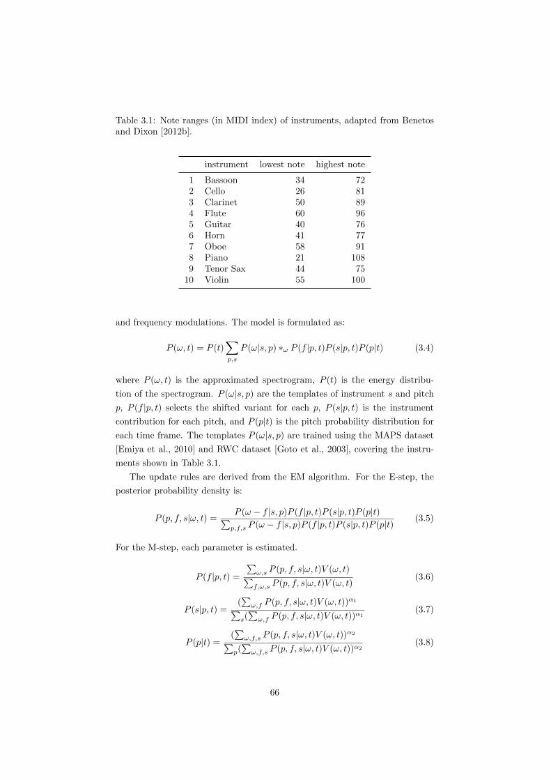
Table 3.1: Note ranges (in MIDI index) of instruments, adapted from Benetosand Dixon [2012b].
instrument lowest note highest note
1 Bassoon 34 722 Cello 26 813 Clarinet 50 894 Flute 60 965 Guitar 40 766 Horn 41 777 Oboe 58 918 Piano 21 1089 Tenor Sax 44 7510 Violin 55 100
and frequency modulations. The model is formulated as:
P (!, t) = P (t)X
p,s
P (!|s, p) ⇤! P (f |p, t)P (s|p, t)P (p|t) (3.4)
where P (!, t) is the approximated spectrogram, P (t) is the energy distribu-
tion of the spectrogram. P (!|s, p) are the templates of instrument s and pitch
p, P (f |p, t) selects the shifted variant for each p, P (s|p, t) is the instrument
contribution for each pitch, and P (p|t) is the pitch probability distribution for
each time frame. The templates P (!|s, p) are trained using the MAPS dataset
[Emiya et al., 2010] and RWC dataset [Goto et al., 2003], covering the instru-
ments shown in Table 3.1.
The update rules are derived from the EM algorithm. For the E-step, the
posterior probability density is:
P (p, f, s|!, t) =P (! � f |s, p)P (f |p, t)P (s|p, t)P (p|t)P
p,f,s P (! � f |s, p)P (f |p, t)P (s|p, t)P (p|t)(3.5)
For the M-step, each parameter is estimated.
P (f |p, t) =
P!,s P (p, f, s|!, t)V (!, t)
Pf,!,s P (p, f, s|!, t)V (!, t)
(3.6)
P (s|p, t) =(P
!,f P (p, f, s|!, t)V (!, t))↵1
Ps(P
!,f P (p, f, s|!, t)V (!, t))↵1(3.7)
P (p|t) =(P
!,f,s P (p, f, s|!, t)V (!, t))↵2
Pp(P
!,f,s P (p, f, s|!, t)V (!, t))↵2(3.8)
66

The templates P (!|s, p) are not updated as they are previously trained and
kept fixed. The parameters ↵1 and ↵2 used in Equation 3.7 and 3.8 are used to
enforce sparsity, where ↵1,↵2 > 1. We follow the original setting, ↵1 = 1.3 and
↵2 = 1.1, from Benetos and Dixon [2012a]. The final piano-roll matrix P (p, t)
and the pitches assigned to each instrument P (p, t, s) are given by:
P (p, t) = P (p|t)P (t) (3.9)
P (p, t, s) = P (s|p, t)P (p|t)P (t) (3.10)
For post-processing, instead of using an HMM, the note events are extracted
by performing thresholding on P (p, t) and using minimum-length pruning (delet-
ing notes shorter than 50ms). The instrument-wise note events are detected in
the same way using P (p, t, s).
3.2.2 The DAEM-based model
Despite using fixed templates, there are still two free parameters, the instrument
contribution and the pitch contribution, to estimate in the baseline method.
They face the risk of converging to local minima. Here, we use the DAEM
algorithm instead of the EM algorithm to derive update rules. In the E-step,
the posterior probability density in Equation 3.5 is modified by introducing a
temperature parameter ⌧ :1
P⌧ (p, f, s|!, t) =(P (! � f |s, p)P (f |p, t)P (s|p, t)P (p|t))1/⌧Pp,f,s(P (! � f |s, p)P (f |p, t)P (s|p, t)P (p|t))1/⌧
(3.11)
And the update rules are extended by adding a ⌧ -loop:
1. Set ⌧ ⌧max(⌧max > 1).
2. Iterate the following EM-steps until convergence:
E-step: calculate P⌧ (p, f, s|!, t).
M-step: estimate P (f |p, t), P (s|p, t) and P (p|t) by replacing P (p, f, s|!, t)
with P⌧ (p, f, s|!, t) in Equation 3.6, 3.7 and 3.8, respectively.
3. Decrease ⌧ .
4. If ⌧ � 1, repeat from step 2; otherwise stop.
The process starts from a high temperature (⌧max > 1), then the temperature
is reduced by gradually decreasing ⌧ . At each value of ⌧ , we apply the EM-
steps until convergence. At higher temperatures, the distributions are smoothed
1The parameter used in [Ueda and Nakano, 1998] is �, and the temperature is indicatedby 1/�. The reason for using ⌧ here is because we want to indicate the temperature directlyby ⌧ and distinguish the proposed method from the �-divergence.
67
and general areas of the search space containing good solutions are found. As
the temperature is gradually decreased, distinctions in the data are sharpened,
resulting in a more fine-grained optimisation at each successive temperature.
Considering the properties of this particular model, we simplify the posterior
probability density to:
P⌧ (p, f, s|!, t) =P (! � f |s, p)P (f |p, t)P (s|p, t)1/⌧P (p|t)P
p,f,s P (! � f |s, p)P (f |p, t)P (s|p, t)1/⌧P (p|t)(3.12)
The convolution of the templates and the pitch impulse distribution, giving the
terms P (!� f |s, p)P (f |p, t), works as the shift-invariant templates here. These
are not modified by the temperature parameter, as the templates are fixed
during the iterative process.2 In addition, having observed that the instrument
distribution P (s|p, t) is dependent on the pitch distribution P (p|t) in this model,
we only modify one of them in the posterior probability density.
In the experiment, the parameter ⌧ took the values 10/i, i 2 {8, 9, 10}.
When ⌧ finally decreases to 1, the update rules agree with the original ones.
3.3 Experiments
3.3.1 Datasets
We used the Bach10 Dataset [Duan et al., 2010] and the MIREX Multi-F0 De-
velopment Dataset (MIREX dataset) [MIREX, 2016] to test the performance
of the proposed method. The Bach10 dataset consists of 10 quartet record-
ings performed on violin, clarinet, saxophone and bassoon. Ground truth for
the Bach10 dataset was automatically generated for each individual instrument
by YIN [de Cheveigne and Kawahara, 2002] with some manual corrections by
Duan and Pardo. The MIREX dataset is an excerpt from a woodwind quintet
recording, played on bassoon, clarinet, flute, horn and oboe. The ground truth
for this dataset was manually created by Benetos and Grindlay.
3.3.2 Evaluation
The performance of the proposed system is evaluated in three subtasks: multiple
F0 estimation, note tracking and instrument assignment. The corresponding
metrics are referred to Section 2.4 for details. We compare the performance
of the proposed method to that of the baseline PLCA model introduced in
Section 3.1 (mentioned as BD(2012) below). We provide results for the three
subtasks on the two di↵erent datasets in the following section.
2This was also confirmed by test experiments where the power 1/⌧ was also applied to thepitch impulse distribution P (f |p, t), giving similar transcription results to Equation 3.12.
68

Table 3.2: Multiple F0 estimation results (see Section 2.4 for explanation ofsymbols).
Dataset Methods P R F Acc Etot Esubs Emiss Efa
Bach10 BD(2012) 0.784 0.791 0.787 0.650 0.311 0.116 0.093 0.102Proposed 0.819 0.796 0.807 0.677 0.282 0.098 0.106 0.078
MIREX BD(2012) 0.748 0.537 0.625 0.455 0.486 0.158 0.305 0.023Proposed 0.769 0.561 0.649 0.480 0.461 0.146 0.292 0.023
Both BD(2012) 0.781 0.768 0.772 0.632 0.327 0.120 0.112 0.094Proposed 0.814 0.775 0.793 0.659 0.299 0.102 0.123 0.074
The proposed system was also submitted to the task of multiple fundamental
frequency estimation and tracking in MIREX 2013.3 Readers are referred to
Table 2.4 for results and comparison to other submissions.
3.3.3 Results
Multiple F0 estimation
The results for multiple F0 estimation using the Bach10 and MIREX datasets
are shown in Table 3.2. It can be seen that the proposed method outperforms
the BD(2012) method in terms of accuracy (Acc) on both individual datasets
by at least 2.5 percentage points, leading to an overall accuracy of 0.659 (up
2.7 percentage points). The total error decreases by 2.8 percentage points. On
the Bach10 dataset improvements are mainly due to a reduced false alarm rate
(Efa), which decreases from 10.2% to 7.8%. This is also reflected by increased
precision (P ) and stable recall (R). The improvement for the MIREX dataset
mainly comes from reduction in both substitution error (Esubs) and missed
detection error (Emiss) rates, leading to higher precision and recall.
In order to determine if the increase in accuracy (Acc) is significant we ran a
Friedman test for this subtask. The resulting p-value of 0.0009 < 0.01 indicates
that the di↵erence is highly significant. The distribution of Acc of the ten files
in the Bach10 dataset is shown in Figure 3.1a.
Note tracking
For the note tracking subtask, we found that the F-measure was improved by
almost 5 percentage points for onset-only evaluation and around 4 percentage
points for onset-o↵set evaluation for both datasets, as shown in Table 3.3. We
ran a Friedman test with regard to the F-measures (Fon and Fo↵) for this
3http://www.music-ir.org/mirex/wiki/2013:Multiple_Fundamental_Frequency_
Estimation_%26_Tracking_Results.
69

Table 3.3: Note-tracking results
(a) onset-only accuracy
Dataset Methods Pon Ron Fon Accon
Bach10 BD(2012) 0.319 0.339 0.328 0.197Proposed 0.399 0.354 0.374 0.231
MIREX BD(2012) 0.628 0.420 0.503 0.336Proposed 0.690 0.459 0.551 0.380
Both BD(2012) 0.347 0.346 0.344 0.209Proposed 0.427 0.364 0.391 0.245
(b) onset and o↵set
Dataset Methods Po↵ Ro↵ Fo↵ Acco↵
Bach10 BD(2012) 0.217 0.230 0.223 0.126Proposed 0.281 0.249 0.263 0.152
MIREX BD(2012) 0.487 0.326 0.391 0.243Proposed 0.537 0.357 0.429 0.273
Both BD(2012) 0.242 0.239 0.238 0.137Proposed 0.305 0.259 0.279 0.163
BD(2012) Proposed
0.61
0.62
0.63
0.64
0.65
0.66
0.67
0.68
0.69
0.7
0.71
(a) Acc
BD(2012) Proposed
0.28
0.3
0.32
0.34
0.36
0.38
0.4
0.42
0.44
0.46
(b) Fon
BD(2012) Proposed
0.18
0.2
0.22
0.24
0.26
0.28
0.3
0.32
0.34
(c) Fo↵
Figure 3.1: Box-and-whisker plots of (a) accuracy; (b) onset-only F-measure;and (c) onset-o↵set F-measure; for the Bach10 dataset.
70
subtask. For both onset-only and onset-o↵set metrics, the p-values are less than
0.01, showing that—here, too—the di↵erences are significant. The distributions
of Fon and Fo↵ for the Bach10 dataset are shown in Figures 3.1b and 3.1c.
The note tracking evaluation shows that both methods under consideration
perform better on the MIREX dataset, whereas according to the frame-based
evaluation they perform better on the Bach10 dataset. This result has the same
trend as the results from other methods on the same data,4 and is likely to stem
from the unusual co-occurrence of trills and legato notes that dominates the
MIREX piece.
Instrument assignment
The results for instrument assignment for the two datasets are shown in Ta-
ble 3.4. In this subtask, we cannot identify a systematic advantage of either
method, with the F-measure means over all instruments being very close (20.7%
and 20.9% on the Bach10 dataset, and 35.1% and 34.3% on the MIREX dataset).
Slight di↵erences between the methods for particular instruments do not show
a consistent advantage of one method either; we will therefore focus on the
proposed method in the rest of the discussion. The most obvious di↵erences in
F-measure occur between instruments. For example, the results for the Bach10
dataset show that instrument assignment works better for the clarinet and bas-
soon than for the violin and saxophone. Also, since the note templates include
instruments not present in the pieces, false positives occur for these instru-
ments, with the largest ratio of false positives occurring for horn (18.6%) and
piano (16.4%). The problem instrument in the MIREX dataset is the oboe, to
which few notes are assigned, leading to a low F-measure of around 12-13%.
Notes are detected in three instruments that do not feature in the music, with
the largest ratio of false positives found in the piano (47.9%) and guitar (34.5%).
No false positives were detected for saxophone or violin.
The discrepancy between the multiple F0 estimation results and the com-
paratively low results for instrument assignment is due to the fact that often the
correct pitch is detected, but assigned to a wrong instrument or combination of
instruments. That is, note templates from di↵erent instruments are combined
to approximate the observed spectra. The proposed method provides a better
reconstruction of the observed data using combinations of templates at the cor-
rect pitches, resulting in better performance for frame level and note tracking
tasks.4as published on the MIREX website [MIREX, 2016].
71

Table 3.4: Instrument assignment results
(a) Bach10
F-measure Violin Clarinet Saxophone Bassoon Mean
BD(2012) 0.175 0.313 0.092 0.246 0.207Proposed 0.190 0.275 0.127 0.243 0.209
(b) MIREX
F-measure Bassoon Clarinet Flute Horn Oboe Mean
BD(2012) 0.292 0.444 0.485 0.409 0.125 0.351Proposed 0.294 0.420 0.489 0.385 0.129 0.343
3.4 Conclusions and discussions
We examine the utility of an optimisation method in a PLCA-based AMT sys-
tem. The optimisation method, deterministic annealing EM, is based on the
EM algorithm and aims to tackle the local minimum problem. The key idea is
to decrease the ‘temperature’ gradually, which means to increase the sparse ex-
ponent gradually in the AMT system. The transcription experiments show that
the proposed method outperforms the baseline method on tasks of multi-pitch
estimation (accuracy increases by 2.7 percentage points) and note tracking (F-
measure increases by 4 percentage points). Although results on an additional
instrument assignment task show no significant di↵erence between the methods,
they reveal that both methods use mixtures of instrument templates to approx-
imate observed spectra in the test data. In this work we have used DAEM
with only one configuration of three temperature steps set by considering the
strategy in [Ueda and Nakano, 1998] and the result of a small preliminary test.
In the future, we would like to explore di↵erent configurations to see whether
we can further improve the transcription results.
In a preliminary experiment, we update both the spectral bases and gain
functions of the basic PLCA model in Equation 3.1 based on DAEM. The cost
function is smaller than that obtained using the EM algorithm, but the tran-
scription results are not always better, because it becomes di�cult to associate
the updated spectral bases to pitches in this case. In comparison to the results
in Section 3.3, we find that the previously-trained templates are important and
work as a good initialisation for the spectral bases. The risk of updating the
templates during the iteration is that an updated template might no longer ac-
cord with its labels (pitch, instrument). Due to the di↵erent ways a note can
be played and di↵erences in sound transmission, templates will never match
observations precisely. Spectral decomposition algorithms compensate for this
72
mismatch by finding mixtures of templates which provide a better approxi-
mation of the data (see Section 3.3.3). In order to capture the variations of
instrument sounds, we would like to refer to information from musical acoustics
and physics. In Chapter 4, we will focus on piano tones to explore the decay
patterns in detail.
The use of the temperature parameter ⌧ that is central to the DAEM algo-
rithm in Equation 3.11 is similar to the use of the sparsity parameters in Equa-
tion 3.7 and Equation 3.8. In fact, the sparsity method used here is related
to the tempered EM algorithm [Grindlay and Ellis, 2012]. Both the DAEM
and sparsity equations ‘put an exponent on a distribution’. When the expo-
nent is larger than one, the distribution becomes sharper and sparser; when the
exponent is smaller than one, the distribution is smoothed, as in the case of
high-temperature stages of DAEM.
The PLCA model is a probabilistic variant of NMF, which is used in a
probabilistic framework. In the remainder of this thesis, we develop our own
transcription approach based on NMF, in consideration of the way that note
energy decays over time. The optimisation method can also be adapted to NMF.
In Chapter 5, we will use this exponential form for a sparsity constraint in an
NMF-based transcription system. The decreasing temperature is indicated by
the increasing exponent. The ‘annealing’ will be applied using a continuously
increasing exponent, which will reach the desired value at the end of iteration.
73
Chapter 4
Modelling the Decay of
Piano Tones
In this chapter, we compare the temporal decay of individual piano partials in
real-world recordings to the theoretical decay patterns based on piano acoustics
revised in Section 2.1.2. We mainly focus on the decay behaviour associated
with coupled piano strings [Weinreich, 1977]. The acoustics of piano decay
is well understood and has been applied for synthesising piano sounds. For
instance, the digital waveguide is used in synthetic models to generate a set
of quasi-harmonic exponentially decaying sinusoids produced by a single string
[Smith, 1992]. A piano note with multiple strings is modelled using coupled
digital waveguides [Aramaki et al., 2001, Bensa et al., 2003], or using one digital
waveguide with resonators for partials of beats and double decay [Bank, 2000,
2001, Lee et al., 2010]. Recently, incorporating the decay information for piano
music analysis has also gained increasing attention. A non-negative source-
filter-decay model is proposed to analyse music sounds by assuming a frequency-
dependent decaying (decay response) [Klapuri, 2007]. The decay envelopes of
piano tones or partials are modelled for automatic music transcription with
promising results [Chen et al., 2012, Berg-Kirkpatrick et al., 2014, Cogliati and
Duan, 2015].
For estimating decay parameters, Valimaki et al. [1996] first propose to
estimate the decay rates of harmonics by linear regression on a logarithmic
magnitude scale. Karjalainen et al. [2002] present both linear and non-linear re-
gressions to estimate the decay of piano partials with noise, but the experiments
only include some examples of synthetic notes and no conclusion is drawn on
the general decay characteristics of piano notes. Here, we track the decay of real
piano tones from the RWC Music Database [Goto et al., 2003] in detail (first 30
74

partials below the Nyquist frequency1 of 88 notes played in 3 dynamics). We
analyse fitness between theoretical models and real world data, and the influence
of the frequency range, pitch range and dynamic on decay patterns. The goal
of this work is to understand piano decay in real recordings and to gain insights
into how piano transcription systems can make use of decay information.
The methods for finding and modelling decays of partials are introduced in
Section 4.1. The experimental setup and results are described in Sections 4.2
and 4.3, respectively. Section 4.4 concludes this chapter.
4.1 Method
In order to track the decay of piano notes, we first find the frequencies of partials
for each note, taking inharmonicity into account. Then, the decay of the partials
is fitted to three typical patterns: linear decay, double decay (modelling the two
directions of polarization, vertical and horizontal) and curves (modelling beats
due to mistuning). We track partials below the Nyquist frequency, but only the
first 30 partials for a note if there are more than 30 partials.
4.1.1 Finding partials
Because of string sti↵ness, partials of piano notes occur at higher frequencies
than the harmonics (integer multiples of the fundamental frequency), which is
known as inharmonicity. The partial frequencies are given by [Fletcher et al.,
1962]:
fn = nf0p
1 +Bn2, (4.1)
where fn is the nth partial of the note with fundamental frequency f0 and B is
the inharmonicity coe�cient which varies from note to note. Moreover, during
the course of a sounded note partial frequencies can diverge from their ideal
inharmonic frequencies due to the coupling between bridge and soundboard.
To get the frequencies of partials, we estimate B and f0 in a non-negative
matrix factorisation framework proposed by Rigaud et al. [2013a]. The model
represents each partial of a piano tone using the main lobe magnitude spectrum
of a Hanning window. In each iteration, the central frequency of each partial
is updated to fit the observed spectrum. An inharmonicity constraint is added
to the cost function by means of a sum of the mean square error between the
estimated partial frequencies and those given by the inharmonicity relation in
Equation 4.1. Then the inharmonicity coe�cient B is also updated by taking
all updated partial frequencies into account. We provide an implementation of
1The Nyquist frequency is half of the sample rate fs.
75

0 500 1000 1500−15
−10
−5
0
Frequency (Hz)
Ampl
itude
(dB)
(a)
30 40 50 60 70 80 90 100
10−4
10−3
10−2
MIDI note index
B (lo
g sc
ale)
(b)
ObservationModelNoise Level
Figure 4.1: (a) Partial frequencies of note A1 (55Hz), (b) Inharmonicity coe�-cient B along the whole compass estimated for the piano of the RWC dataset.
this method for download.2 When detecting frequencies of partials, errors are
likely to arise at partials below the noise level, and even when the frequencies
of these partials are detected correctly, they tend to behave noisily. So only
partials above the noise level are tracked.
Figure 4.1(a) shows the detected frequencies of the first 30 partials of the note
A1 (55Hz). The estimated inharmonicity coe�cient along the piano compass
(all 88 piano notes) is given in Figure 4.1(b).
4.1.2 Tracking the decay of partials
The vibrations of the strings are influenced by many factors, which results in a
variety of decay patterns of piano notes. We fit the decay of partials with the
following three models: linear decay, multi-phase linear decay, and non-linear
2https://code.soundsoftware.ac.uk/projects/inharmonicityestimation
76

curve decay based on the theoretical analysis of coupled oscillation of two piano
strings [Weinreich, 1977]. Partial decay of notes with three strings is also fitted
by these three models.
Linear decay is suitable for partials of single string notes, notes with well-
tuned strings and also notes with large mistunings, with examples shown in
Figure 4.2. Multi-phase linear decay is mainly used for double decay caused
by transmission direction changes and mistuned strings. It can also be applied
for partials with fast decay. In this case, the partial decays to the noise level
quickly, and the noisy part is detected as a second line, as shown in Figure 4.3.
Partials of notes with mistuned strings exhibit a decay with beats, and is fitted
by the non-linear curvy decay. Some high partials of single-string notes also
exhibit a decaying periodic curve because of false beating. Readers are referred
to Section 2.1.2 for related information on piano decay.
Time-frequency representation
A piano tone starts with a percussive sound with a sharp increase of energy
generated by the impact of the hammer on the string(s). In order to to discard
the attack onset, we use a sound clip beginning at the frame with largest energy
for each note. In the RWC dataset [Goto et al., 2003], each piano note lasts about
2 seconds. The length of the clip is set to 2 s, while if the clip is shorter than
2 s the length is restricted to its duration. The sampling rate is fs = 44100Hz.
Frames are segmented by a 4096-sample Hamming window with a hop-size of
441. A discrete Fourier Transform is performed on each frame with 2-fold zero-
padding. The power spectrogram is represented on the log scale:
SdB = 20 log10(S), (4.2)
where S is the magnitude spectrogram.
The energy of each partial is found according to the frequencies detected in
Section 4.1.1. Then the decays are fitted by the following models. The decay
rate is measured by the power change per second (dB/s).
Linear regression
In most situations, the decay of partials follows a linear function of time, which
is modelled by
y(t) = at+ b, (4.3)
where y is the linear function along time t, a is the decay rate and b is the initial
power. The regression parameters are estimated using ordinary least squares.
Figure 4.2 shows three kinds of decay which can be fitted in the linear model:
77
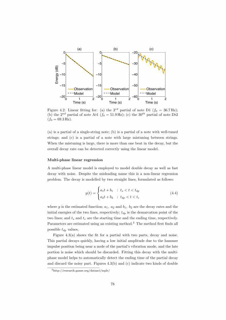
0 1 2−20
−15
−10
−5
0(a)
Time (s)
Ener
gy (d
B)
ObservationModel
0 1 2−20
−15
−10
−5
0(b)
Time (s)
ObservationModel
0 1 2−60
−50
−40
−30
−20(c)
Time (s)
ObservationModel
Figure 4.2: Linear fitting for: (a) the 3rd partial of note D1 (f0 = 36.7Hz);(b) the 2nd partial of note A[1 (f0 = 51.9Hz); (c) the 30th partial of note D[2(f0 = 69.3Hz).
(a) is a partial of a single-string note; (b) is a partial of a note with well-tuned
strings; and (c) is a partial of a note with large mistuning between strings.
When the mistuning is large, there is more than one beat in the decay, but the
overall decay rate can be detected correctly using the linear model.
Multi-phase linear regression
A multi-phase linear model is employed to model double decay as well as fast
decay with noise. Despite the misleading name this is a non-linear regression
problem. The decay is modelled by two straight lines, formulated as follows:
y(t) =
8<
:a1t+ b1 : ts < t < tdp
a2t+ b2 : tdp < t < te(4.4)
where y is the estimated function; a1, a2 and b1, b2 are the decay rates and the
initial energies of the two lines, respectively; tdp is the demarcation point of the
two lines; and ts and te are the starting time and the ending time, respectively.
Parameters are estimated using an existing method.3 The method first finds all
possible tdp values,
Figure 4.3(a) shows the fit for a partial with two parts, decay and noise.
This partial decays quickly, having a low initial amplitude due to the hammer
impulse position being near a node of the partial’s vibration mode, and the late
portion is noise which should be discarded. Fitting this decay with the multi-
phase model helps to automatically detect the ending time of the partial decay
and discard the noisy part. Figures 4.3(b) and (c) indicate two kinds of double
3http://research.ganse.org/datasci/mplr/
78

0 1 2−80
−60
−40
−20
0(a)
Time (s)
Ener
gy (d
B)
ObservationModel
0 1 2−80
−60
−40
−20
0(b)
Time (s)
ObservationModel
0 1 2−80
−60
−40
−20
0(c)
Time (s)
ObservationModel
Figure 4.3: Multi-phase linear fitting for: (a) the 7th partial of note B[0 (f0 =29.1Hz); (b) the 4th partial of note B[2 (f0 = 116.5Hz); (c) the 1st partial ofnote E5 (f0 = 659.3Hz).
decay. The rate change in (b) is caused by the transmission direction switching
from vertical to horizontal, while the reason for the double decay in (c) is a
small frequency di↵erence between the strings.
For double decay, the slope of the line which covers the larger part of the
time duration is recorded as the decay rate, i.e. the first part in Figure 4.3(b)
and the second part in Figure 4.3(c). We assume that the decay lasts longer
than noise in the situation of fast decay with noise, so the larger part strategy
also works in this case, i.e. the first decay rate in Figure 4.3(a).
Non-linear curve fitting
When there are small frequency di↵erences between the strings of a note, partials
decay with amplitude modulation as the vibrations of the di↵erent strings move
in and out of phase with each other. We use a non-linear curve fitting model to
fit these decays with beats. The objective function of the curve fitting is more
complex than the first two situations. Based on the theory of coupled strings
[Weinreich, 1977], the formula is simplified as follows:
y(t) = at+ b+A log10(| cos(ft+ ')|+ "). (4.5)
The derivation from the physical model [Weinreich, 1977] to the proposed model
is included in Appendix A. This function describes the coupled motion of two
strings. There are two parts: the decay part is still modelled by a linear function,
at+ b, and the remaining term models the amplitude modulation, where A and
f are the amplitude and frequency of the curve, respectively. ' is the initial
phase of the curve, and " = 0.01 is added to avoid taking the log of 0.
79

0 1 2−80
−60
−40
−20
0(a)
Time (s)
Ener
gy (d
B)
ObservationModel
0 1 2−80
−60
−40
−20
0(b)
Time (s)
ObservationModel
0 1 2−80
−60
−40
−20
0(c)
Time (s)
ObservationModel
Figure 4.4: Non-linear curve fitting for: (a) the 22nd partial of note D[1 (f0 =34.6Hz); (b) the 10th partial of note G1 (f0 = 49Hz); and (c) the 10th partialof note A1 (f0 = 55Hz).
Figure 4.4 gives three examples of decay with beats: (a) false beats of a high
partial of a single string note; (b) and (c) show beats with di↵erent frequencies,
which are caused by mistuning of the strings of each note.
The parameters are estimated using a non-linear least squares algorithm [Fox
and Weisberg, 2010]. This method requires a good initialisation and ranges for
parameters to get a reasonable result. The linear part (a, b) is initialised using
the result of the linear model. The amplitude A is initialised to 40 which is
the amplitude of purely resistive coupling in dB, as shown in Appendix A.
The period (1/f) consists of two lobes because of taking the absolute value in
Equation 4.5. If there is more than one trough found in the decay, as shown in
Figure 4.4(a) and (b), we initialise the curve period to be double the time gap
between two adjacent troughs. If only one trough is detected (Figure 4.4(c)),
we assume the position of the trough from the onset to be one quarter of the
period. The initial phase ' is usually initialised to 0, while sometimes manually
adjusted to a value between 0 and ⇡ according to the observation.
The coupling between 3 strings is far more complex than for 2 strings. It
is out of the scope of this chapter to explore the details of the motion of 3
strings, which we approximate using the models described above. It turns out
that the approximation is very close to our observations, as shown in the results
of Section 4.3.
4.2 Experiment
In this section, we introduce the dataset, metric for evaluation and the steps of
decay modelling.
80
4.2.1 Dataset
We use the piano sounds from the RWC Musical Instrument Sound Database
[Goto et al., 2003]. The notes are played at three dynamics: loud (forte, f ),
moderate (mezzo, m) and soft (piano, p). Each set consists of 88 isolated notes,
covering the whole compass of the piano.
4.2.2 Metric
The coe�cient of determination (R-squared) is used for evaluating the fit be-
tween the data and model. It is defined as follows:
R2 = 1�SS res
SS tot= 1�
PTt=1(ot � yt)2PTt=1(ot � o)2
, (4.6)
where ot is the observation of time frame t, yt is the modelled function and
o = 1T
PTt=1 ot is the mean of the observations. SS tot is the total sum of squares,
which is proportional to the variance of the observed data, and SS res is the
residual sum of squares, explaining the di↵erence between the observations and
the modelled values. The larger R-squared is, the better the data is explained
by the model.
4.2.3 Modelling the decay
For each detected partial, we fit it to our models according to the process shown
in Figure 4.5. The process is referred to as the mixed model, in which the R2 of
the three models is computed one by one. We first compute the R2s of the linear
model and the multi-phase linear model. If the larger R2 of these two models
is over 0.9, we assume the decay is fitted well and no curve fitting is needed.
Otherwise, we continue to compute the R2 of the non-linear curve model. We
find the largest R2 of the three models as the R2 of the mixed model.
4.3 Results
We illustrate the results of decay tracking in this section. Then the estimated
decay rates are used to parameterise the decay response and to explore the
influence of dynamics.
4.3.1 R-squared
We compare the average coe�cient of determination, R2, between the linear
model and the combination of all three models (referred to as the mixed model
81

Set 𝑅12, 𝑅22, 𝑅32=0
Linear regression
Calculate 𝑅12
Multi-phase linear regression
Calculate 𝑅22𝑅2 =max(𝑅12, 𝑅22)
𝑅2>0.90?
Curve fitting
Calculate 𝑅32
𝑅2 =Max(𝑅12, 𝑅22, 𝑅32)
END
Yes
No
Figure 4.5: Flowchart of partial decay modelling.
Table 4.1: Average R2 of the linear and mixed models. NP is the number ofpartials above the noise level for each dynamic level.
Dynamics NP linear model mixed model
f 1572 0.721 0.867m 1501 0.699 0.853p 1187 0.644 0.824
as in Figure 4.5). The results are presented in Table 4.1, which indicate that
the mixed model has a better fit to the data by around 15 percentage points.
We also note that the performance is influenced by dynamics. If the note starts
at a lower energy, it will decay to the noise level more quickly, resulting in
fewer data available for modelling, not only fewer partials above the noise level,
but also shorter duration of notes. This reduction in data makes parameter
estimation more di�cult, resulting in worse performance for lower dynamics.
Although longer notes would help us to observe the decay pattern, we did not
look beyond 2 s, which is already longer than the duration of most notes in
normal music performance. It remains to be investigated how well our model
performs on shorter notes.
In order to provide a more detailed investigation of the results for di↵erent
notes, we divide the notes into 8 groups, with every adjacent 11 notes in a group.
The average R2 of each group is shown in Figure 4.6. We find that the mixed
82
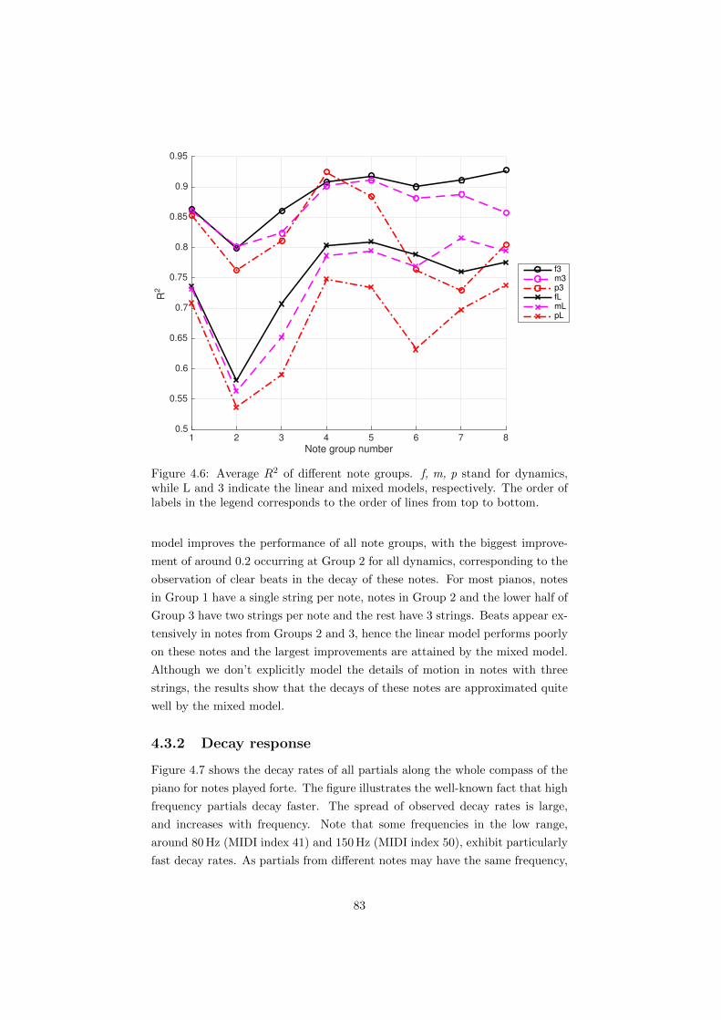
1 2 3 4 5 6 7 8Note group number
0.5
0.55
0.6
0.65
0.7
0.75
0.8
0.85
0.9
0.95R
2
f3m3p3fLmLpL
Figure 4.6: Average R2 of di↵erent note groups. f, m, p stand for dynamics,while L and 3 indicate the linear and mixed models, respectively. The order oflabels in the legend corresponds to the order of lines from top to bottom.
model improves the performance of all note groups, with the biggest improve-
ment of around 0.2 occurring at Group 2 for all dynamics, corresponding to the
observation of clear beats in the decay of these notes. For most pianos, notes
in Group 1 have a single string per note, notes in Group 2 and the lower half of
Group 3 have two strings per note and the rest have 3 strings. Beats appear ex-
tensively in notes from Groups 2 and 3, hence the linear model performs poorly
on these notes and the largest improvements are attained by the mixed model.
Although we don’t explicitly model the details of motion in notes with three
strings, the results show that the decays of these notes are approximated quite
well by the mixed model.
4.3.2 Decay response
Figure 4.7 shows the decay rates of all partials along the whole compass of the
piano for notes played forte. The figure illustrates the well-known fact that high
frequency partials decay faster. The spread of observed decay rates is large,
and increases with frequency. Note that some frequencies in the low range,
around 80Hz (MIDI index 41) and 150Hz (MIDI index 50), exhibit particularly
fast decay rates. As partials from di↵erent notes may have the same frequency,
83

30 40 50 60 70 80 90 100 110 120Log frequency (MIDI note index)
-120
-100
-80
-60
-40
-20
0D
eca
y ra
te (
dB
/s)
Figure 4.7: Decay response: decay rates against frequency. Lower values meanfaster decay. The greyscale is used to indicate fundamental frequency, withdarker colours corresponding to lower pitches.
di↵erent decay rates of these partials could be used as a clue to decide which note
the partial belongs to. However, in musical performances, overlapped partials
increase the di�culty of tracking partial decay, which is a topic needing further
investigation.
4.3.3 Decay of di↵erent dynamics
Figure 4.8 shows the decay rates of the first five partials of notes played at
di↵erent dynamics. We observe that dynamics have no significant absolute
e↵ect on the decay rate. In the low pitch range, the decay rates of di↵erent
dynamics are almost identical, while in the high pitch range this is less clear,
partly due to higher measurement error because of fewer data for modelling.
4.4 Conclusions
We model the decay of piano notes based on piano acoustics theory. Two non-
linear models (a multi-phase linear model and a non-linear curve fitting model)
are used to fit double decay and beats of piano tone partials, respectively. The
results show that the use of non-linear models provides a better fit to the data,
especially for notes in the low register. The decay response of the piano shows
84
that decay increases with frequency. The results also indicate that dynamics
have no significant e↵ect on the decay rate.
Based on the observation that linear regression fits data with R2⇡ 70%
and works well for notes in the middle and high pitch ranges, we assume an
exponential decay in the next chapter for piano transcription. According to
analysis on decay response and dynamic influence, notes of di↵erent pitches will
be modelled with di↵erent decay rates, while notes of the same pitch played by
di↵erent dynamics share the same decay rate.
In [Cheng et al., 2015a], we track the decay after 200 ms of the onsets. We
think that 200 ms is too long for high-pitch notes, because they decay quickly.
In this chapter, we use the sound clip starting from the frame with the largest
energy for each note. We apply the model twice on slightly di↵erent data,
and get similar results and conclusions. We believe that the proposed model is
reproducible by following the method described in Section 4.1. For future work,
to extend the model to other instruments, such as guitar, harpsichord and harp,
would also be a good topic to explore.
85

30 40 50 60 70 80 90 100 110 120-100
-80
-60
-40
-20
0
De
cay
rate
(d
B/s
)
the 1st partial
fmp
30 40 50 60 70 80 90 100 110 120-100
-80
-60
-40
-20
0
De
cay
rate
(d
B/s
)
the 2nd partial
fmp
30 40 50 60 70 80 90 100 110 120-100
-80
-60
-40
-20
0
De
cay
rate
(d
B/s
)
the 3rd partial
fmp
30 40 50 60 70 80 90 100 110 120-100
-80
-60
-40
-20
0
De
cay
rate
(d
B/s
)
the 4th partial
fmp
30 40 50 60 70 80 90 100 110 120Log frequency (MIDI note index)
-100
-80
-60
-40
-20
0
De
cay
rate
(d
B/s
)
the 5th partial
fmp
Figure 4.8: Decay rates for the first five partials for di↵erent dynamics
86

Chapter 5
An Attack/Decay Model for
Piano Transcription
In this chapter, we demonstrate that piano transcription performance for a
known piano can be improved by explicitly modelling piano acoustical features.
The proposed method is based on non-negative matrix factorisation, with the
following three refinements: (1) introduction of attack and harmonic decay com-
ponents; (2) use of a spike-shaped note activation that is shared by these com-
ponents; (3) modelling the harmonic decay with an exponential function. Tran-
scription is performed in a supervised way, with the training and test datasets
produced by the same piano.
Several features associated with piano acoustics, such as inharmonicity, time-
varying timbre and decaying energy, are examined for their utilities for tran-
scription. Rigaud et al. [2013b] show that an explicit inharmonicity model leads
to improvement in piano transcription, while a note-dependent inharmonicity
parameter is needed for initialisation. Modelling time-varying timbre not only
provides a better reconstruction of the spectrogram, but also improves note
tracking results by imposing constraints between note stages (attack, sustain
and decay) [Benetos et al., 2013a, Cheng et al., 2015b]. For decaying energy,
Chen et al. [2012]’s preliminary work uses an exponential model for energy evo-
lution of notes. Berg-Kirkpatrick et al. [2014] represent the energy evolution
of a piano note by a trained envelope. Ewert et al. [2015] represent both time-
varying timbre and temporal evolution of piano notes by time-frequency patches.
Temporal evolution modelling allows a note event to be represented by a sin-
gle amplitude parameter for its whole duration, enabling the development of
note-level systems with promising transcription results [Chen et al., 2012, Berg-
Kirkpatrick et al., 2014, Ewert et al., 2015]. In addition, Cogliati and Duan
87
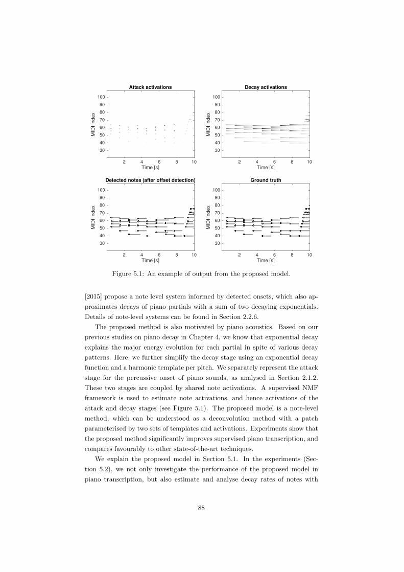
Attack activations
2 4 6 8 10Time [s]
30
40
50
60
70
80
90
100M
IDI in
dex
Decay activations
2 4 6 8 10Time [s]
30
40
50
60
70
80
90
100
MID
I in
dex
Detected notes (after offset detection)
2 4 6 8 10Time [s]
30
40
50
60
70
80
90
100
MID
I in
dex
Ground truth
2 4 6 8 10Time [s]
30
40
50
60
70
80
90
100
MID
I in
dex
Figure 5.1: An example of output from the proposed model.
[2015] propose a note level system informed by detected onsets, which also ap-
proximates decays of piano partials with a sum of two decaying exponentials.
Details of note-level systems can be found in Section 2.2.6.
The proposed method is also motivated by piano acoustics. Based on our
previous studies on piano decay in Chapter 4, we know that exponential decay
explains the major energy evolution for each partial in spite of various decay
patterns. Here, we further simplify the decay stage using an exponential decay
function and a harmonic template per pitch. We separately represent the attack
stage for the percussive onset of piano sounds, as analysed in Section 2.1.2.
These two stages are coupled by shared note activations. A supervised NMF
framework is used to estimate note activations, and hence activations of the
attack and decay stages (see Figure 5.1). The proposed model is a note-level
method, which can be understood as a deconvolution method with a patch
parameterised by two sets of templates and activations. Experiments show that
the proposed method significantly improves supervised piano transcription, and
compares favourably to other state-of-the-art techniques.
We explain the proposed model in Section 5.1. In the experiments (Sec-
tion 5.2), we not only investigate the performance of the proposed model in
piano transcription, but also estimate and analyse decay rates of notes with
88

di↵erent dynamics. Conclusions are drawn in Section 5.3.
5.1 Method
The method is composed of three main steps. We first introduce the attack and
decay model for piano sounds. Parameters are estimated using a sparse NMF.
The second step is to detect onsets from the attack activations by peak-picking.
In the third step, o↵sets are detected for each pitch individually. Below we
explain each step in turn.
5.1.1 A model of attack and decay
A piano sound is produced by a hammer hitting the string(s) of a key [Weinreich,
1977]. It starts with a large energy, then decays till the end of the note. At the
attack stage, the strike of the hammer produces a percussive sound. It evolves
quickly to an almost harmonic pitched sound, and then immediately enters the
decay stage. We define a generative model for these two phases individually, in
which the attack sound is generated by:
V aft =
KX
k=1
W afkH
akt, (5.1)
where Va is the reconstructed spectrogram of the attack phase, as shown in
Figure 5.2(d), and Wa is the percussive template (Figure 5.2(e)). f 2 [1, F ]
is the frequency bin, t 2 [1, T ] indicates the time frame, and k 2 [1,K] is the
pitch index. The attack activations Ha (Figure 5.2(c)) are formulated by a
convolution:
Hakt =
t+TaX
⌧=t�Ta
Hk⌧P (t� ⌧), (5.2)
where H are spike-shaped note activations, shown in Figure 5.2(b), and P is
the amplitude attack envelope, with the typical shape shown in Figure 5.5. The
range of the attack envelope is determined by the overlap for computing the
spectrogram, with Ta equal to the overlap ratio (the ratio of the window size
and frame hop size).
For the decay part we assume that piano notes decay approximately ex-
ponentially based on studies in Chapter 4. The harmonic decay is generated
by
V dft =
KX
k=1
W dfkH
dkt, (5.3)
where Vd is the reconstructed spectrogram of the decay phase (Figure 5.2(g)),
89
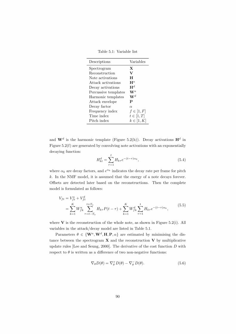
Table 5.1: Variable list
Descriptions Variables
Spectrogram XReconstruction VNote activations HAttack activations Ha
Decay activations Hd
Percussive templates Wa
Harmonic templates Wd
Attack envelope PDecay factor ↵Frequency index f 2 [1, F ]Time index t 2 [1, T ]Pitch index k 2 [1,K]
and Wd is the harmonic template (Figure 5.2(h)). Decay activations Hd in
Figure 5.2(f) are generated by convolving note activations with an exponentially
decaying function:
Hdkt =
tX
⌧=1
Hk⌧e�(t�⌧)↵k , (5.4)
where ↵k are decay factors, and e↵k indicates the decay rate per frame for pitch
k. In the NMF model, it is assumed that the energy of a note decays forever.
O↵sets are detected later based on the reconstructions. Then the complete
model is formulated as follows:
Vft = V aft + V d
ft
=KX
k=1
W afk
t+TaX
⌧=t�Ta
Hk⌧P (t� ⌧) +KX
k=1
W dfk
tX
⌧=1
Hk⌧e�(t�⌧)↵k ,
(5.5)
where V is the reconstruction of the whole note, as shown in Figure 5.2(i). All
variables in the attack/decay model are listed in Table 5.1.
Parameters ✓ 2 {Wa,Wd,H,P,↵} are estimated by minimising the dis-
tance between the spectrogram X and the reconstruction V by multiplicative
update rules [Lee and Seung, 2000]. The derivative of the cost function D with
respect to ✓ is written as a di↵erence of two non-negative functions:
r✓D(✓) = r+✓ D(✓)�r�
✓ D(✓). (5.6)
90
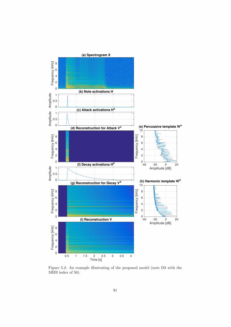
(a) Spectrogram X
0
2
4
6
8
Fre
quency
[kH
z]
0
0.5
1
Am
plit
ude
(b) Note activations H
0
0.5
1
Am
plit
ude
(c) Attack activations Ha
(d) Reconstruction for Attack Va
0
2
4
6
8
Fre
quency
[kH
z]
0
2
4
6
8
10
Fre
quency
[kH
z]
-40 -20 0 20Amplitude [dB]
(e) Percussive template Wa
0
0.5
1
Am
plit
ude
(f) Decay activations Hd
(g) Reconstruction for Decay Vd
0
2
4
6
8
Fre
quency
[kH
z]
0
2
4
6
8
10
Fre
quency
[kH
z]
-40 -20 0 20Amplitude [dB]
(h) Harmonic template Wd
(i) Reconstruction V
0.5 1 1.5 2 2.5 3 3.5 4Time [s]
0
2
4
6
8
Fre
quency
[kH
z]
Figure 5.2: An example illustrating of the proposed model (note D3 with theMIDI index of 50).
91
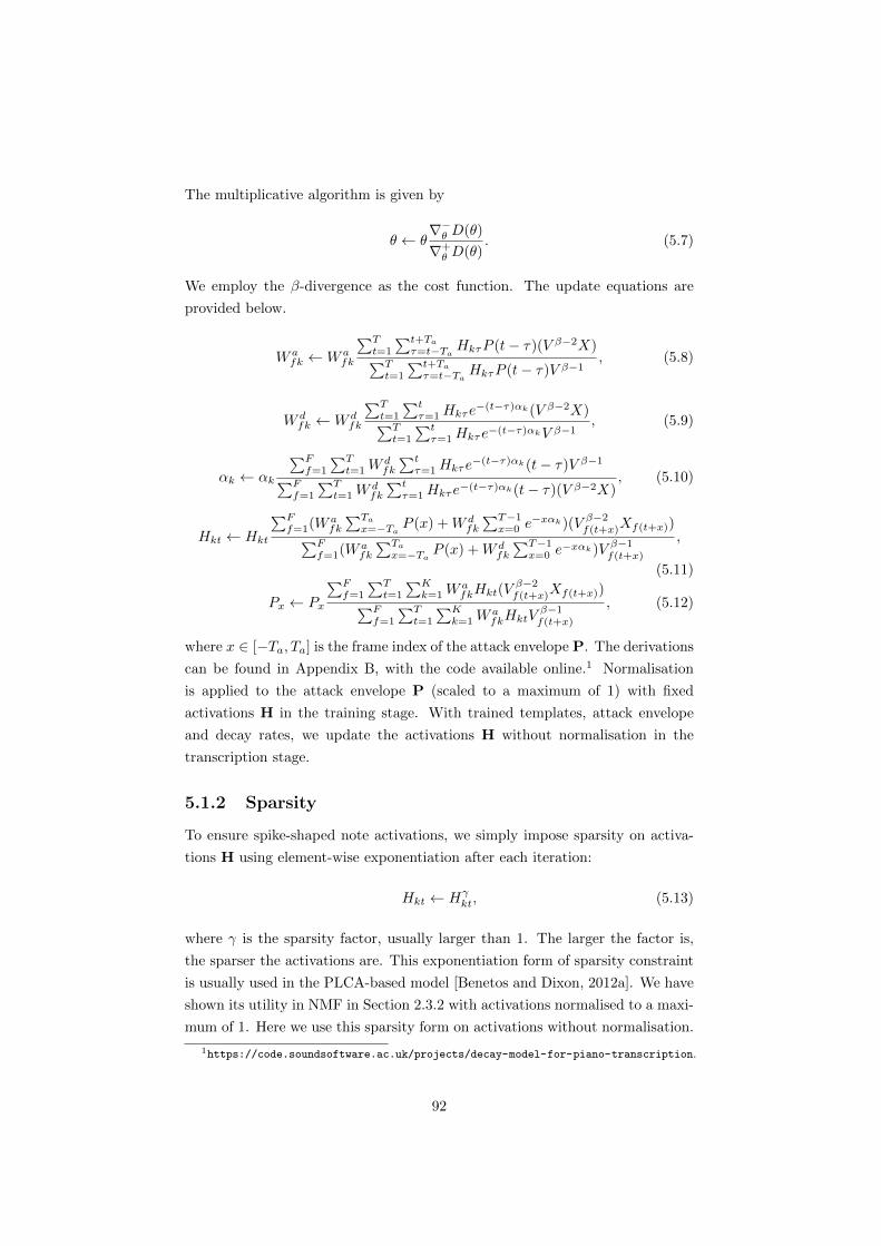
The multiplicative algorithm is given by
✓ ✓r
�✓ D(✓)
r
+✓ D(✓)
. (5.7)
We employ the �-divergence as the cost function. The update equations are
provided below.
W afk W a
fk
PTt=1
Pt+Ta
⌧=t�TaHk⌧P (t� ⌧)(V ��2X)
PTt=1
Pt+Ta
⌧=t�TaHk⌧P (t� ⌧)V ��1
, (5.8)
W dfk W d
fk
PTt=1
Pt⌧=1 Hk⌧e
�(t�⌧)↵k(V ��2X)PT
t=1
Pt⌧=1 Hk⌧e�(t�⌧)↵kV ��1
, (5.9)
↵k ↵k
PFf=1
PTt=1 W
dfk
Pt⌧=1 Hk⌧e
�(t�⌧)↵k(t� ⌧)V ��1
PFf=1
PTt=1 W
dfk
Pt⌧=1 Hk⌧e�(t�⌧)↵k(t� ⌧)(V ��2X)
, (5.10)
Hkt Hkt
PFf=1(W
afk
PTa
x=�TaP (x) +W d
fk
PT�1x=0 e�x↵k)(V ��2
f(t+x)Xf(t+x))PF
f=1(Wafk
PTa
x=�TaP (x) +W d
fk
PT�1x=0 e�x↵k)V ��1
f(t+x)
,
(5.11)
Px Px
PFf=1
PTt=1
PKk=1 W
afkHkt(V
��2f(t+x)Xf(t+x))
PFf=1
PTt=1
PKk=1 W
afkHktV
��1f(t+x)
, (5.12)
where x 2 [�Ta, Ta] is the frame index of the attack envelope P. The derivations
can be found in Appendix B, with the code available online.1 Normalisation
is applied to the attack envelope P (scaled to a maximum of 1) with fixed
activations H in the training stage. With trained templates, attack envelope
and decay rates, we update the activations H without normalisation in the
transcription stage.
5.1.2 Sparsity
To ensure spike-shaped note activations, we simply impose sparsity on activa-
tions H using element-wise exponentiation after each iteration:
Hkt H�kt, (5.13)
where � is the sparsity factor, usually larger than 1. The larger the factor is,
the sparser the activations are. This exponentiation form of sparsity constraint
is usually used in the PLCA-based model [Benetos and Dixon, 2012a]. We have
shown its utility in NMF in Section 2.3.2 with activations normalised to a maxi-
mum of 1. Here we use this sparsity form on activations without normalisation.
1https://code.soundsoftware.ac.uk/projects/decay-model-for-piano-transcription.
92

In this case, sparsity is enforced by increasing activations above 1 and decreasing
activations below 1.
A preliminary test confirmed that the number of peaks in activations de-
creases as the degree of sparsity increases. We also apply an annealing sparsity
factor similar to Chapter 3, which means a continuously changing factor. We
set � to increase from 1 to �a 2 [1.01, 1.05] gradually within the iterations.
5.1.3 Onset detection
Di↵erent playing styles and overlapping between notes may cause a mismatch
between the observed attack energy and the trained attack envelope. This re-
sults in multiple peaks around onsets in the activations. Figures 5.3(a) and (b)
show note activations and attack activations of pitch G2 in a music excerpt,
respectively. Attack activations indicate the actual attack envelopes of notes
obtained by the proposed model. We detect onsets from attack activations by
peak-picking [Wang et al., 2008]. First, we compute smoothed attack activa-
tions for each pitch, using a moving average filter with a window of 20 bins.
Only peaks which exceed the smoothed attack activations by a threshold will
be retained as onset candidates, as shown in Figure 5.3(b). The threshold is
adapted to each piece with the parameter �
Thre = �maxk,t
Hak,t. (5.14)
We test various � 2 {�21dB,�22dB, . . . ,�40dB} in the experiment.
We find that there are still double peaks around onsets after thresholding.
In order to deal with this problem, we simply merge pairs of peaks which are too
close to each other. We set the minimal interval between two successive notes
of the same pitch to be 0.1 second. If the interval between two peaks is smaller
than the minimal interval, we generate a new peak. The time index of the new
peak is a weighted average (weighted by amplitudes) of the indices of the two
peaks, while its amplitude is the sum of that of the two peaks. Figure 5.3 (c)
shows detected onsets after merging double peaks. We apply the above process
again to get rid of triple peaks.
5.1.4 O↵set detection
We adapt the method of Ewert et al. [2015] to detect the o↵sets by dynamic
programming. For each pitch, there are two states s 2 {0, 1}, denoting state
93

7 8 9 10 11 12 13 14Time [s]
0
0.02
0.04
0.06
0.08
0.1
Am
plit
ud
e
(a) Note activations H
7 8 9 10 11 12 13 14Time [s]
0
0.05
0.1
0.15
0.2
Am
plit
ud
e
Smoothed attack activaitonsSmoothed attack activations + thresholdOnset candidates
(b) Attack activations Ha, showing median filtering and peak selection
7 8 9 10 11 12 13 14Time [s]
0
0.1
0.2
0.3
Am
plit
ud
e
(c) Detected onsets, showing result of merging of close onsets
Figure 5.3: Example of onset detection showing how activations are processed.
94
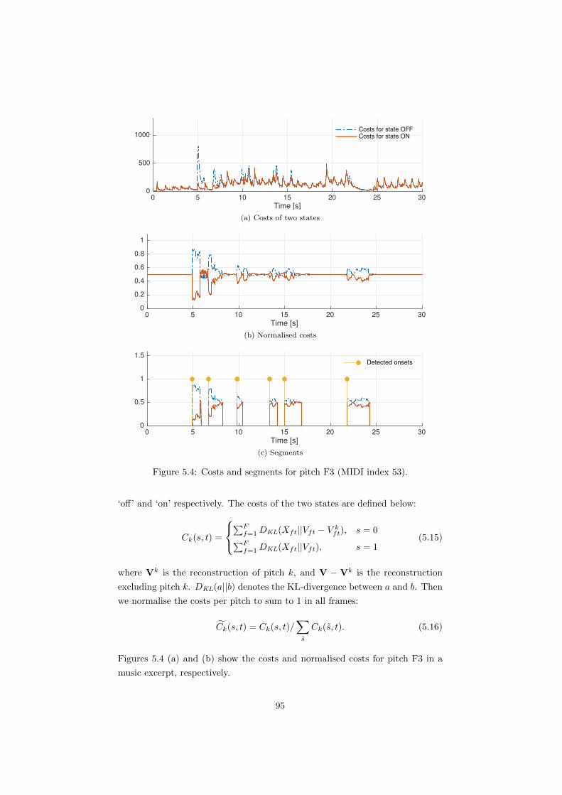
0 5 10 15 20 25 30Time [s]
0
500
1000Costs for state OFFCosts for state ON
(a) Costs of two states
0 5 10 15 20 25 30Time [s]
0
0.2
0.4
0.6
0.8
1
(b) Normalised costs
0 5 10 15 20 25 30Time [s]
0
0.5
1
1.5Detected onsets
(c) Segments
Figure 5.4: Costs and segments for pitch F3 (MIDI index 53).
‘o↵’ and ‘on’ respectively. The costs of the two states are defined below:
Ck(s, t) =
8<
:
PFf=1 DKL(Xft||Vft � V k
ft), s = 0PF
f=1 DKL(Xft||Vft), s = 1(5.15)
where Vk is the reconstruction of pitch k, and V � Vk is the reconstruction
excluding pitch k. DKL(a||b) denotes the KL-divergence between a and b. Then
we normalise the costs per pitch to sum to 1 in all frames:
fCk(s, t) = Ck(s, t)/X
s
Ck(s, t). (5.16)
Figures 5.4 (a) and (b) show the costs and normalised costs for pitch F3 in a
music excerpt, respectively.
95

We can find the optimal state sequence by applying dynamic programming
on the normalised costs. First, we recursively calculate the accumulated costs
from the previous states to the current state. The smaller accumulated cost at
each step gives the cost of the optimal path to each state, which is stored in an
accumulated cost matrix:
Ak(s, t) =
8<
:mins2{0,1}(Ak(s, t� 1) + fCk(s, t)w(s, s)), t > 1
fCk(s, t), t = 1(5.17)
where w is the weight matrix. In our experiment, the weights are
w =
"0.5 0.55
0.55 0.5
#,
which favours self-transitions, in order to obtain a smoother sequence. The
indices of the optimal path are stored in the matrix E as follows:
Ek(s, t) = arg mins2{0,1}
(Ak(s, t� 1) + fCk(s, t)w(s, s)), t > 1 (5.18)
Then we trace back the optimal path from the end of sequence, with the optimal
states given by
Sk(t) =
8<
:argmins2{0,1} Ak(s, t), t = T
Ek(Sk(t+ 1), t+ 1), t 2 [1, T � 1](5.19)
We find that when the activation of the pitch is 0 or very small, the costs
of the two states are the same or very close, and no state transition occurs. In
these frames, the pitch state is expected to be o↵, but dynamic programming
can not jump out from the previous state. Then it will be detected as state on.
In order to deal with this problem we need to exclude these parts before applying
dynamic programming. Figure 5.4(c) shows the segmentation by detected onsets
and the costs. Each segment starts at a detected onset and ends when the
di↵erence of the smoothed normalised costs is less than a set threshold (0.05 in
our experiment). We track the states of the pitch for each segment individually.
5.2 Experiments
This section is organised as follows. Experiments are described in Section 5.2.1.
We analyse performance of the proposed model with di↵erent sparsity factors
in Section 5.2.2, and compare to state-of-the-art methods in Section 5.2.3. In
Section 5.2.4, an unsupervised transcription is applied on repeated notes of
96
single piano pitches to analyse performance of the proposed model in di↵erent
pitch ranges and dynamics. Decay rates of isolated piano notes of di↵erent
dynamics are compared in Section 5.2.5.
5.2.1 Experimental setup
We use audio files sampled at 44100Hz. To compute the spectrogram, frames
are segmented by a 4096-sample Hamming window with a hop-size of 882.2 A
discrete Fourier transform is performed on each frame with 2-fold zero-padding.
To lessen the influence of beats in the decay stage [Cheng et al., 2015a], we
smooth the spectrogram with a median filter covering 5 time frames (100ms).
During parameter estimation, we use the KL-divergence (� = 1) as the cost
function. The proposed model is iterated for 50 times in all experiments to
achieve convergence.
Datasets
The experiments are performed on three datasets, consisting of sounds from a
real piano (‘ENSTDkCl’) and a synthetic piano (‘AkPnCGdD’) in the MAPS
database [Emiya et al., 2010], and another 10 synthetic piano pieces (denoted
as ‘PianoE’)3 [Ewert et al., 2015]. Piano sounds in the ENSTDkCl subset are
recorded on a Disklavier piano. Piano sounds in the AkPnCGdD subset and Pi-
anoE dataset are synthesised using the Native Instruments Akoustik Piano and
Native Instruments Vienna Concert Grand VST plugins, respectively. The main
transcription experiment in Section 5.2.2 uses pieces in the ENSTDkCl subset,
and the comparison experiment in Section 5.2.3 is performed on pieces in all
three datasets. Both experiments use the first 30 seconds of each piece and train
parameters on isolated notes produced by the same piano in the test dataset.
In Section 5.2.4 the proposed method is used to detect onsets of repeated notes
of single pitches in the ENSTDkCl subset. We analyse decay rates of isolated
notes in three dynamics also in the ENSTDkCl subset in Section 5.2.5. Datasets
used in di↵erent experiments are summarised in Table 5.2.
5.2.2 The main transcription experiment
The training stage
We train percussive and harmonic templates, decay rates and the attack enve-
lope on the isolated notes. Note activations are updated with other parameters
2A 20ms hop size is used to reduce computation time. For frame-wise evaluation, tran-scription results are represented with a hop size of 10ms by duplicating every frame.
3http://www.piano-e-competition.com.
97

Table 5.2: Datasets used in the experiments
Experiment Datasets
Main transcription (Section 5.2.2) ENSTDkCl (music pieces)Comparison experiment (Section 5.2.3) ENSTDkCl, AkPnCGdD
and PianoE (music pieces)Unsupervised transcription (Section 5.2.4) ENSTDkCl (repeated notes)Decay rate analysis (Section 5.2.5) ENSTDkCl (isolated notes)
Table 5.3: Experimental configuration for the training stage
Round one Round two
Initialisation InitialisationWd: random Wd: randomWa, ↵, P: all ones Wa, ↵: all ones
P: mean of the results of round oneH: set based on the ground truth H: set based on the ground truth
update Wd, Wa, ↵, P update Wd, Wa, ↵
Parameters ParametersK = 1 same as leftsparsity: unavailable
fixed.4
The training stage includes two rounds, as shown in Table 5.3. In the first
round, we first fix note activations (H) for each isolated note according to the
ground truth, then update all other parameters (Wa, Wd, P and ↵). The attack
envelopes are normalised to a maximum of 1 after each iteration. The attack
envelopes follow a certain shape and can be shared by all pitches. So we use
the average of the trained attack envelopes to reduce the number of parameters
and to avoid potential overfitting. The trained attack envelopes and the average
attack envelope are shown in Figure 5.5. In the second round, we fix the note
activations (H) and the average attack envelope (P), then update all other
parameters (Wa, Wd and ↵).
Transcription results
For transcription, we update note activations H, keeping parameters Wa, Wd,
P and ↵ fixed from the training stage. Note activations are updated using
Equation 5.11 with di↵erent sparsity factors. The experimental configuration is
shown in Table 5.4. Onset-only note tracking results (presented as percentages)
are shown in Table 5.5 with di↵erent sparsity factors. The last column indicates
4The proposed model runs at about 3 ⇥ real-time using MATLAB on a MacBook Prolaptop (I7, 2.2GHz, 16GB).
98

-4 -2 0 2 4Frame index
0
0.2
0.4
0.6
0.8
1A
mp
litu
de
(a) Attack envelopes for all notes
-4 -2 0 2 4Frame index
0
0.2
0.4
0.6
0.8
1
Am
plit
ud
e
(b) Average attack envelope
Figure 5.5: Attack envelopes.
Table 5.4: Experimental configuration I for the transcription experiments inSection 5.2.2.
InitialisationWd, Wa, ↵, P: trainedH: random
update H only
ParametersK = 88sparsity: � range from 1 to 1.05onset threshold: optimal threshold
the optimal thresholds. We find that all F-measures with di↵erent sparsity fac-
tors are above 80% with optimal thresholds, and the optimal threshold decreases
when sparsity increases. The top part of Table 5.5 contains results using fixed
sparsity factors. The best results are achieved without the sparsity constraint
(� = 1.00), with an F-measure of 82.24%. The performance decreases with in-
creasing sparsity factor. When the sparsity factor equals 1.05, the F-measure
drops to 80.51%. The second part of the experiment gives results for using an-
nealing sparsity. The best F-measure is 82.36% with the setting (1.00 ! 1.02)
and the worst F-measure is 81.76% with the setting (1.00 ! 1.05). The di↵er-
ence between the best and the worst F-measure is only 0.6 percentage points.
In general, results with annealing sparsity are slightly better than those with
fixed sparsity.
Figure 5.6 shows attack activations and detected onsets for di↵erent sparsity
factors for pitch G4 for the first 10 seconds of a piano piece. Note activations are
normalised to a maximum activation of 1 in that piece. With a small sparsity
factor, there are more peaks in attack activations, and it is more likely to have
false positives, as shown in Figure 5.6(a). In Figure 5.6(b), due to the high spar-
sity constraint, small peaks are more likely to disappear, resulting in an extra
missed detected note (around 8 seconds). False positive peaks can be discarded
99

Table 5.5: Note tracking results with di↵erent fixed sparsity factors (above) andannealing sparsity factors (below).
� Pon Ron Fon Aon �(dB)
1.00 88.52 77.70 82.24 70.54 -291.01 87.70 78.18 82.23 70.53 -301.02 87.67 77.36 81.80 69.87 -301.03 87.22 77.31 81.62 69.66 -311.04 86.95 76.84 81.26 69.17 -321.05 86.38 75.99 80.51 68.14 -33
1 ! 1.01 87.77 78.08 82.18 70.49 -301 ! 1.02 88.49 77.79 82.36 70.73 -301 ! 1.03 88.22 77.78 82.27 70.60 -311 ! 1.04 87.86 77.66 82.09 70.35 -321 ! 1.05 86.83 77.83 81.76 69.84 -34
in the onset detection stage by thresholding and merging onsets. On the other
hand if peaks disappear by imposing sparsity, they can not be recovered at later
stages.
We compute the performance using thresholds ranging from �40 to �21dB
to study how performance changes with the change of thresholds. Figure 5.7(a)
shows the results for di↵erent fixed sparsity factors. It is clear that precision
decreases with the increase of the threshold, while recall increases. The higher
the sparsity factor is, the more robust the results are to threshold changes.
When decreasing the threshold from the optimal value to smaller values (moving
towards �40dB), the F-measure drops from above 82% to below 75% without
sparsity, while the di↵erence in F-measure is within 2 percentages when � =
1.05. This is because small peaks in activations are already discounted when
imposing sparsity. Lowering the threshold does not bring many false positives.
Results with higher sparsity are less sensitive to reduction in the threshold.
However, when the threshold becomes larger, the results with low sparsity still
outperform those with high sparsity. With a larger threshold, the number of
true positives decreases. There are more peaks in activations when using lower
sparsity, so more true positives remain. This favours the assumption that the
true positives have larger amplitudes. Figure 5.7(b) shows the robustness of
using annealing sparsity factors. The transcription results are close to each
other. With annealing sparsity, the results are better and more tolerant to
threshold changes. The sparser the factor is, the robuster the result is to low
thresholds. The reductions in F-measure for di↵erent sparsity factors are similar
to those of the fixed sparsity when the threshold is increased.
100

1 2 3 4 5 6 7 8 9 10Time [s]
0
0.5
1
1.5
2
Am
plit
ude
Attack activationsGround TruthDetected onsets
(a) Attack activations (� = 1.01)
1 2 3 4 5 6 7 8 9 10Time [s]
0
0.5
1
1.5
2
Am
plit
ude
Attack activationsGround TruthDetected onsets
(b) Attack activations (� = 1.05)
Figure 5.6: Detected onsets with di↵erent sparsity for pitch G4 (MIDI index67).
101

0.65 0.7 0.75 0.8 0.85 0.9 0.95 1
Precision
0.6
0.65
0.7
0.75
0.8
0.85
0.9
Recall
1.00
1.01
1.02
1.03
1.04
1.05
F-measure = 0.85
F-measure = 0.75
(a) Results with fixed sparsity factors
0.65 0.7 0.75 0.8 0.85 0.9 0.95 1
Precision
0.6
0.65
0.7
0.75
0.8
0.85
0.9
Recall
1->1.01
1->1.02
1->1.03
1->1.04
1->1.05
F-measure = 0.85
F-measure = 0.75
(b) Results with annealing sparsity factors
Figure 5.7: Performance using di↵erent sparsity factors and thresholds. Thesparsity factors are indicated by di↵erent shapes, as shown in the legends. Linesconnecting di↵erent shapes are results achieved via the same threshold. Thethreshold of the top-left set is �40dB, and the bottom-right set is �21dB. Thedashed lines show F-measure contours, with the values decreasing from top-rightto bottom-left.
102
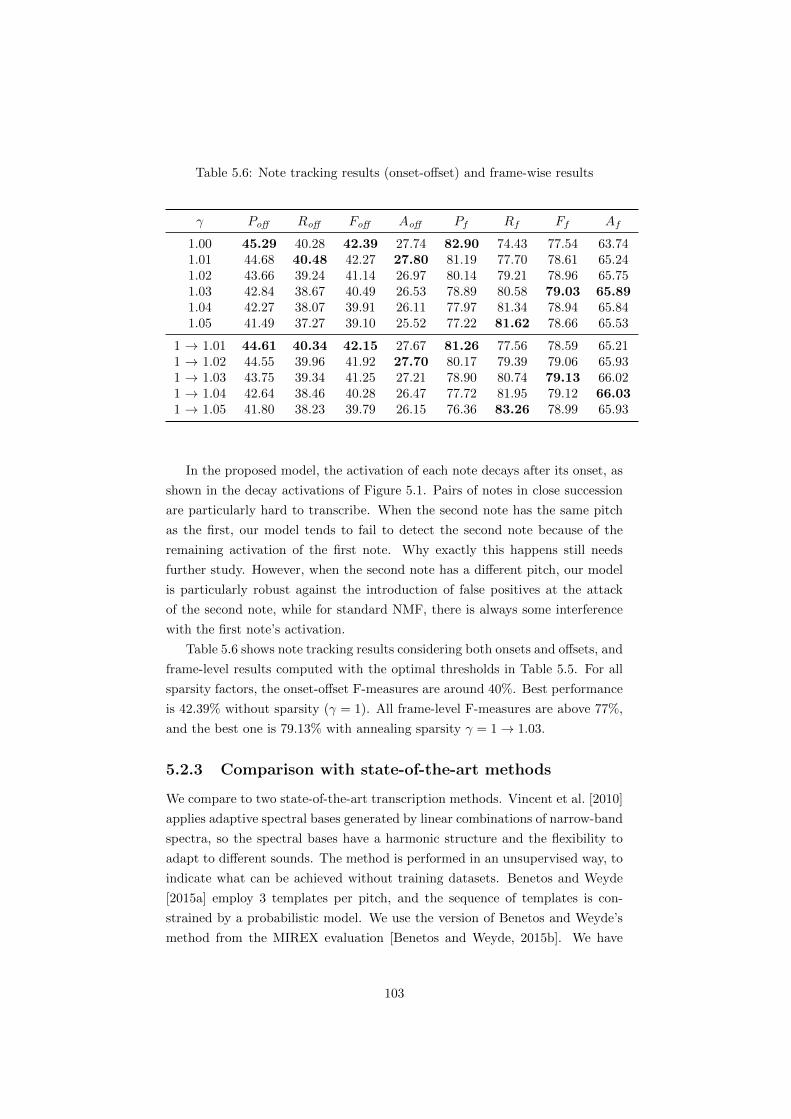
Table 5.6: Note tracking results (onset-o↵set) and frame-wise results
� Po↵ Ro↵ Fo↵ Ao↵ Pf Rf Ff Af
1.00 45.29 40.28 42.39 27.74 82.90 74.43 77.54 63.741.01 44.68 40.48 42.27 27.80 81.19 77.70 78.61 65.241.02 43.66 39.24 41.14 26.97 80.14 79.21 78.96 65.751.03 42.84 38.67 40.49 26.53 78.89 80.58 79.03 65.891.04 42.27 38.07 39.91 26.11 77.97 81.34 78.94 65.841.05 41.49 37.27 39.10 25.52 77.22 81.62 78.66 65.53
1 ! 1.01 44.61 40.34 42.15 27.67 81.26 77.56 78.59 65.211 ! 1.02 44.55 39.96 41.92 27.70 80.17 79.39 79.06 65.931 ! 1.03 43.75 39.34 41.25 27.21 78.90 80.74 79.13 66.021 ! 1.04 42.64 38.46 40.28 26.47 77.72 81.95 79.12 66.031 ! 1.05 41.80 38.23 39.79 26.15 76.36 83.26 78.99 65.93
In the proposed model, the activation of each note decays after its onset, as
shown in the decay activations of Figure 5.1. Pairs of notes in close succession
are particularly hard to transcribe. When the second note has the same pitch
as the first, our model tends to fail to detect the second note because of the
remaining activation of the first note. Why exactly this happens still needs
further study. However, when the second note has a di↵erent pitch, our model
is particularly robust against the introduction of false positives at the attack
of the second note, while for standard NMF, there is always some interference
with the first note’s activation.
Table 5.6 shows note tracking results considering both onsets and o↵sets, and
frame-level results computed with the optimal thresholds in Table 5.5. For all
sparsity factors, the onset-o↵set F-measures are around 40%. Best performance
is 42.39% without sparsity (� = 1). All frame-level F-measures are above 77%,
and the best one is 79.13% with annealing sparsity � = 1! 1.03.
5.2.3 Comparison with state-of-the-art methods
We compare to two state-of-the-art transcription methods. Vincent et al. [2010]
applies adaptive spectral bases generated by linear combinations of narrow-band
spectra, so the spectral bases have a harmonic structure and the flexibility to
adapt to di↵erent sounds. The method is performed in an unsupervised way, to
indicate what can be achieved without training datasets. Benetos and Weyde
[2015a] employ 3 templates per pitch, and the sequence of templates is con-
strained by a probabilistic model. We use the version of Benetos and Weyde’s
method from the MIREX evaluation [Benetos and Weyde, 2015b]. We have
103

access to the code and train templates on isolated notes of the corresponding
pianos. In the PianoE dataset, we also compare to the method of Ewert et al.
[2015]. This method identifies frames in NMD patterns with states in a dy-
namical system. Note events are detected with constant amplitudes but various
durations. The method uses template patterns trained on isolated notes. We
only have access to the published data in [Ewert et al., 2015].
Based on our previous analysis, we employ the following parameters for the
proposed model in comparison experiments. The sparsity factor is � = 1 !
1.04 by balancing among transcription results and the robustness to di↵erent
thresholds. Onsets are detected with threshold � = �30dB. In the first dataset
(ENSTDkCl), results of other methods are also reported with optimal thresholds
with best note-wise F-measures. Then the same thresholds are used for the two
synthetic piano datasets.
Results on piano pieces from the ENSTDkCl subset are shown in Ta-
ble 5.7(a). The proposed model has a note tracking F-measure of 81.80% and
a frame-wise F-measure of 79.01%, outperforming Vincent et al.’s unsupervised
method by around 10 and 20 percentage points, respectively. Results of Benetos
and Weyde’s method are in between.
Results on the synthetic piano AkPnCGdD are shown in Table 5.7(b). In
general, all methods perform better on this dataset than on the ‘ENSTDkCl’
dataset, especially on note tracking results. The proposed model has the best re-
sults (84.63% on note tracking F-measure and 80.81% on frame-wise F-measure),
outperforming all other methods by at least 5 percentage points.
Results on the other synthetic dataset PianoE are shown in Table 5.7(c).
Compared to the other datasets, note tracking results of all methods are good
but frame-wise results are poor. Ewert et al.’s method performs the best on
note tracking (88% on F-measure), and Benetos and Weyde’s method is the
second (83.80% on F-measure). The proposed model only outperforms Vincent
et al.’s method, with F-measures of 81.28% and 79.41% for these two methods
respectively. However, the proposed model remains the best on the frame-wise
F-measure (66.77%). Pieces in this dataset are from a piano competition. Many
notes have very short durations. The remaining energies of a short note in the
proposed model may interfere with later notes, causing false negatives.
A supervised neural network model also has been tested on the MAPS
database for piano transcription [Sigtia et al., 2016]. Besides an acoustic model,
the method employs a music language model to capture the temporal structure
of music. Although the method is not directly comparable, it is noticeable that
our method exceeds its results by at least 5 percentage points on F-measures.
When tested on the real recordings using templates trained on the synthetic pi-
ano notes, the proposed method has both frame-level and note-level F-measures
104
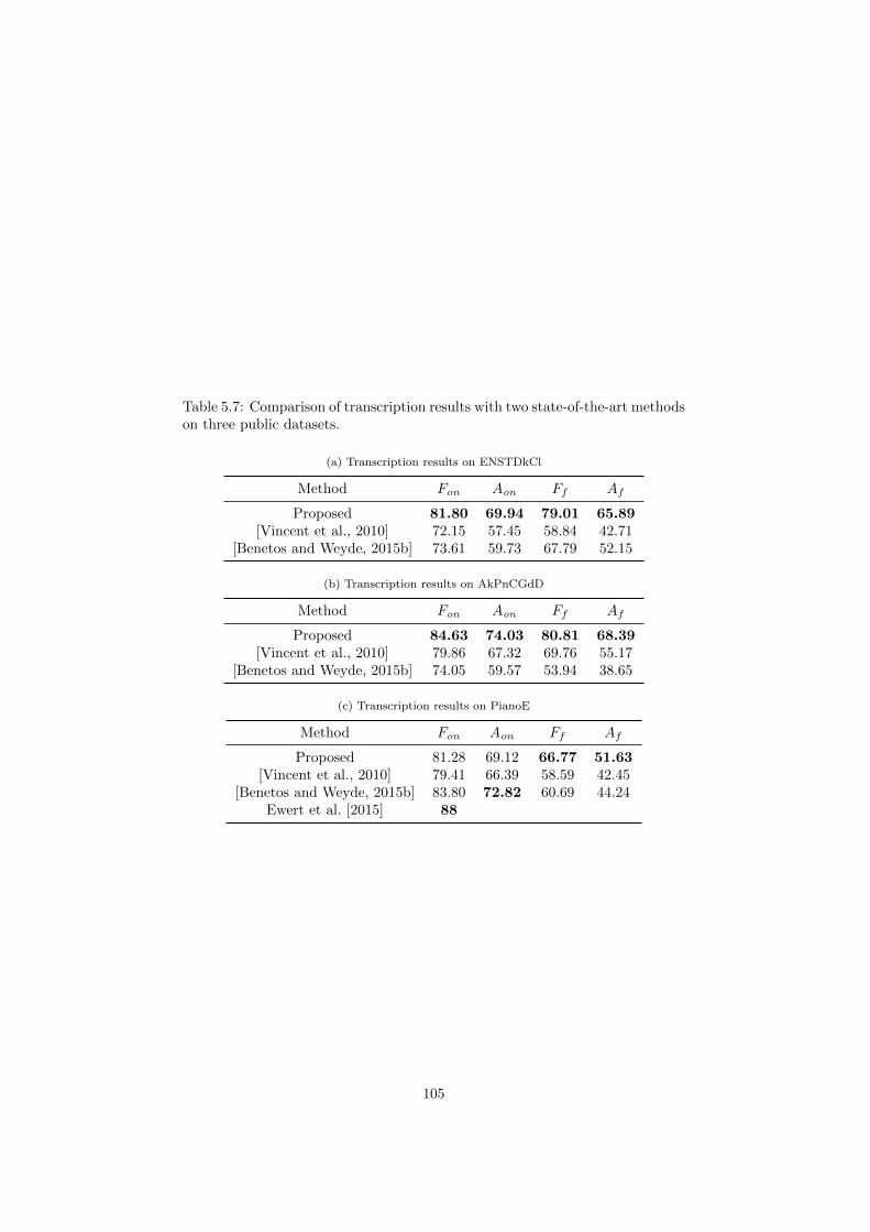
Table 5.7: Comparison of transcription results with two state-of-the-art methodson three public datasets.
(a) Transcription results on ENSTDkCl
Method Fon Aon Ff Af
Proposed 81.80 69.94 79.01 65.89[Vincent et al., 2010] 72.15 57.45 58.84 42.71
[Benetos and Weyde, 2015b] 73.61 59.73 67.79 52.15
(b) Transcription results on AkPnCGdD
Method Fon Aon Ff Af
Proposed 84.63 74.03 80.81 68.39[Vincent et al., 2010] 79.86 67.32 69.76 55.17
[Benetos and Weyde, 2015b] 74.05 59.57 53.94 38.65
(c) Transcription results on PianoE
Method Fon Aon Ff Af
Proposed 81.28 69.12 66.77 51.63[Vincent et al., 2010] 79.41 66.39 58.59 42.45
[Benetos and Weyde, 2015b] 83.80 72.82 60.69 44.24Ewert et al. [2015] 88
105

Table 5.8: Experimental configuration II for test on repeated notes in Sec-tion 5.2.4.
InitialisationWd, H: randomWa, ↵, P: all ones
update all
ParametersK = 1sparsity: � = 1! 1.04onset threshold: � = �30dB
of around 65%, outperforming the method of Sigtia et al. [2016] by 10 percentage
points on note-wise F-measure in a similar experiment.
5.2.4 Test on repeated notes for single pitches
We investigate the proposed model’s performance on di↵erent dynamics and
pitches in this experiment. We use 66 sound clips generated according to MIDI
files using the Disklavier piano in the subset ‘ENSTDkCl’ of the MAPS database
[Emiya et al., 2010]. Each of the clips consists of about 15 notes of a single pitch.
Notes in one clip have the same MIDI velocity, and repeat faster and faster. The
larger the velocity is, the louder the sound is. The sound clips are divided into
three dynamics: forte (loud), mezzo-forte (moderately loud) and piano (soft),
with 22 clips in each of three dynamics.
The experimental configuration for this experiment is shown in Table 5.8.
The activations are normalised to be the maximum of 1 after each iteration.
We adopt the optimal parameters from the previous transcription experiment.
All variables are updated during the iterations. We focus on onset-only note
tracking results in this experiment. Information in some clips with soft notes is
not aligned with the sounds. We manually correct onsets of these clips5 referring
to results of the onset detection method SuperFlux [Bock and Widmer, 2013].
Table 5.9 shows detailed results of note tracking (onset-only) of repeated
notes. We list the numbers of true positives, false positives and false negatives
rather than precision, recall to give an intuitive aspect on the results. In general,
the proposed model can find most onsets, indicated by small numbers of false
negatives. The results are better for loud or moderately loud notes, with average
F-measures of 88.53% and 85.38% respectively. In these two dynamics, many
false positives are detected in the low pitch range, while there are few false
5The manually corrected onsets are given in the following linkhttps://code.soundsoftware.ac.uk/projects/decay-model-for-piano-transcription.
106

positives for notes in the middle and high pitch ranges (above MIDI index 50).
When notes are quiet, the average F-measure is smallest (76.61%). There is no
certain trend for performance associated with pitch ranges.
Figure 5.8 shows some examples of pitches in low and high range, which are
played in three dynamics. There are many false positives for low pitches, as
shown in the left sub-figures, possibly caused by time-varying timbre (beating
especially [Cheng et al., 2015a]), reverberation and so on. There are less false
positives for quiet low-pitch notes, as shown on the left of Figure 5.8(c). We
find that some peaks appear around o↵sets of notes. This is the sound of the
damper coming into contact with the string. This sound and the remaining
energy are easy to be detected as another quiet note. The system works quite
well for notes of high pitches, as shown in the right sub-figures. Most onsets are
correct and clearly detected. There are false positives around the o↵sets for the
quiet high-pitch note on the right of Figure 5.8(c). At the end of these clips,
notes are repeated very fast. We can find that some of these notes are merged
into one note, resulting in some false negatives.
In this experiment, we analyse the performance of the proposed model in
di↵erent dynamics and pitch ranges. Firstly, we find the di↵erences of perfor-
mance on notes in di↵erent dynamics. The louder the notes are, the better the
model performs. Secondly, the proposed model works better for notes in the
middle and high pitch ranges. As indicated in the results of Section 4.3.1, the
exponential decay has the worst results to fit the decay of tones in low pitch
range because of the beats. This can be one reason for the bad performance
for the low pitch range of the proposed model. Thirdly, the proposed model
tends to merge fast-repeated notes into one note. This kind of false negatives is
largely related to the simplification of ignoring note o↵sets at the first stage.
107

Tab
le5.9:
Notetracking(onset-on
ly)resultsforrepeatednotes
indi↵erentdyn
amics.
Forte
Mezzo-forte
Piano
Pitch
Ntp
Nfp
Nfn
FPitch
Ntp
Nfp
Nfn
FPitch
Ntp
Nfp
Nfn
F
2113
102
68.42
2213
82
72.22
2111
40
84.62
3013
132
63.41
2412
93
66.67
228
161
48.48
3111
144
55.00
2614
131
66.67
3210
60
76.92
3713
42
81.25
2713
82
72.22
3811
40
84.62
4414
41
84.85
2812
93
66.67
4911
50
81.48
4513
32
83.87
2913
82
72.22
5010
70
74.07
4913
02
92.86
3613
62
76.47
5211
30
88.00
5313
02
92.86
5214
21
90.32
5412
50
82.76
5514
31
87.50
6213
22
86.67
5713
20
92.86
5913
02
92.86
6314
01
96.55
6110
131
58.82
6614
01
96.55
6614
11
93.33
639
112
58.06
7114
11
93.33
6814
21
90.32
6710
111
62.50
7214
01
96.55
7714
11
93.33
6911
00
100.00
7513
02
92.86
8114
01
96.55
7212
22
85.71
7913
12
89.66
8313
12
89.66
7410
50
80.00
8414
01
96.55
8913
22
86.67
7911
30
88.00
8814
01
96.55
9314
01
96.55
8410
50
80.00
9214
01
96.55
9614
01
96.55
938
84
57.14
9414
01
96.55
100
130
292
.86
9612
00
100.00
102
140
196
.55
103
140
196
.55
100
100
010
0.00
103
140
196
.55
107
122
382
.76
107
74
366
.67
105
140
196
.55
108
140
196
.55
108
49
634
.78
Average
F-m
easure
88.53
85.38
76.61
108
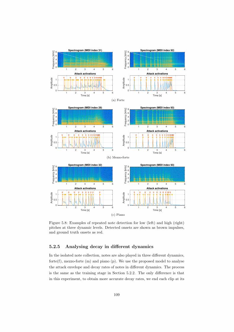
Spectrogram (MIDI index 31)
1 2 3 4 5 60
2
4
6
8F
req
ue
ncy
[kH
z]
1 2 3 4 5 6Time [s]
0
0.5
1
Am
plit
ud
e
Attack activations
Spectrogram (MIDI index 92)
1 2 3 4 5 60
2
4
6
8
Fre
qu
en
cy [
kHz]
1 2 3 4 5 6Time [s]
0
0.5
1
Am
plit
ud
e
Attack activations
(a) Forte
Spectrogram (MIDI index 29)
1 2 3 4 5 60
2
4
6
8
Fre
qu
en
cy [
kHz]
1 2 3 4 5 6Time [s]
0
0.5
1
Am
plit
ud
e
Attack activations
Spectrogram (MIDI index 93)
1 2 3 4 5 60
2
4
6
8
Fre
qu
en
cy [
kHz]
1 2 3 4 5 6Time [s]
0
0.5
1
Am
plit
ud
e
Attack activations
(b) Mezzo-forte
Spectrogram (MIDI index 32)
1 2 3 4 5 60
2
4
6
8
Fre
qu
en
cy [
kHz]
1 2 3 4 5 6Time [s]
0
0.5
1
Am
plit
ud
e
Attack activations
Spectrogram (MIDI index 93)
1 2 3 4 5 60
2
4
6
8
Fre
qu
en
cy [
kHz]
1 2 3 4 5 6Time [s]
0
0.5
1
Am
plit
ud
e
Attack activations
(c) Piano
Figure 5.8: Examples of repeated note detection for low (left) and high (right)pitches at three dynamic levels. Detected onsets are shown as brown impulses,and ground truth onsets as red.
5.2.5 Analysing decay in di↵erent dynamics
In the isolated note collection, notes are also played in three di↵erent dynamics,
forte(f), mezzo-forte (m) and piano (p). We use the proposed model to analyse
the attack envelope and decay rates of notes in di↵erent dynamics. The process
is the same as the training stage in Section 5.2.2. The only di↵erence is that
in this experiment, to obtain more accurate decay rates, we end each clip at its
109
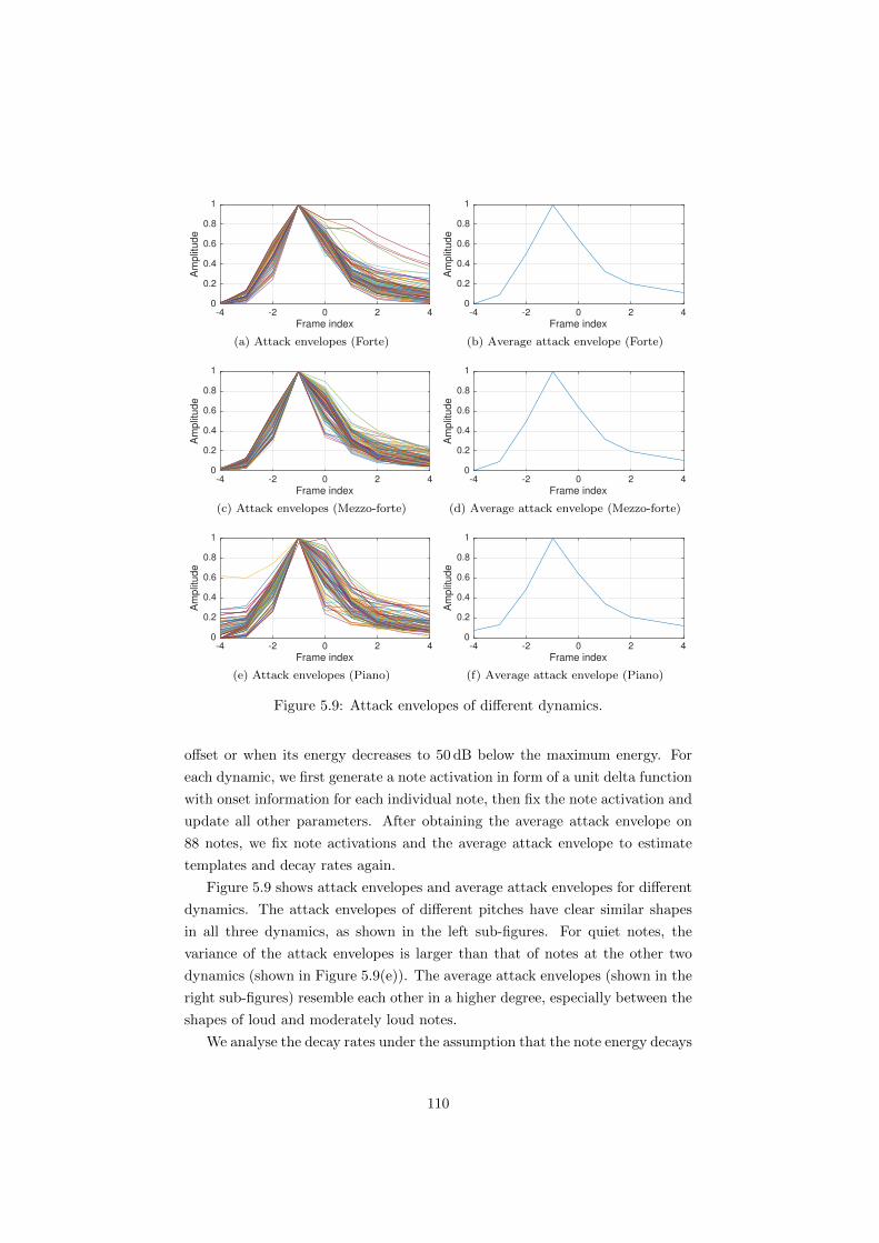
-4 -2 0 2 4Frame index
0
0.2
0.4
0.6
0.8
1A
mp
litu
de
(a) Attack envelopes (Forte)
-4 -2 0 2 4Frame index
0
0.2
0.4
0.6
0.8
1
Am
plit
ud
e
(b) Average attack envelope (Forte)
-4 -2 0 2 4Frame index
0
0.2
0.4
0.6
0.8
1
Am
plit
ud
e
(c) Attack envelopes (Mezzo-forte)
-4 -2 0 2 4Frame index
0
0.2
0.4
0.6
0.8
1
Am
plit
ud
e
(d) Average attack envelope (Mezzo-forte)
-4 -2 0 2 4Frame index
0
0.2
0.4
0.6
0.8
1
Am
plit
ud
e
(e) Attack envelopes (Piano)
-4 -2 0 2 4Frame index
0
0.2
0.4
0.6
0.8
1
Am
plit
ud
e
(f) Average attack envelope (Piano)
Figure 5.9: Attack envelopes of di↵erent dynamics.
o↵set or when its energy decreases to 50 dB below the maximum energy. For
each dynamic, we first generate a note activation in form of a unit delta function
with onset information for each individual note, then fix the note activation and
update all other parameters. After obtaining the average attack envelope on
88 notes, we fix note activations and the average attack envelope to estimate
templates and decay rates again.
Figure 5.9 shows attack envelopes and average attack envelopes for di↵erent
dynamics. The attack envelopes of di↵erent pitches have clear similar shapes
in all three dynamics, as shown in the left sub-figures. For quiet notes, the
variance of the attack envelopes is larger than that of notes at the other two
dynamics (shown in Figure 5.9(e)). The average attack envelopes (shown in the
right sub-figures) resemble each other in a higher degree, especially between the
shapes of loud and moderately loud notes.
We analyse the decay rates under the assumption that the note energy decays
110

30 40 50 60 70 80 90 100MIDI index
0
10
20
30
40
50
60D
eca
y ra
te [dB
/s]
FMP
Figure 5.10: Decay rates as a function of pitch for di↵erent dynamics.
exponentially. For notes played forte, there is a trend that higher pitched notes
decay faster, as shown in the blue circles in Figure 5.10. For notes of the other
two dynamics, the trend is less clear. When comparing decay rates of the same
pitch, we find that in the low pitch range (below 50 in MIDI index), the decay
rates of the notes at di↵erent dynamics are close to each other. Dynamics barely
influence decay in this pitch range. The decay rates corresponding to di↵erent
dynamics begin to vary for the notes in the following two octaves. In the high
pitch range (MIDI indices above 74), there are obvious di↵erences among the
decay rates, with the notes with higher energy decaying faster, while there is
still more consistency in decay rates of the same note in comparison to that of
other notes.
This experiment is to verify the assumption that notes of the same pitch de-
cay at the same rate despite dynamics. The result suggests that this assumption
is suitable for notes in the low and middle pitch ranges, but not for high-pitch
notes.
5.3 Conclusion and future work
In this chapter we propose an attack/decay model for piano transcription. We
model a piano note as having a percussive attack stage and a harmonic de-
111

cay stage, and the decay stage is explicitly modelled as an exponential decay.
Parameters are learned using a sparse NMF, and transcription is performed
in a supervised way. We detect onsets on attack activations by peak-picking
and track pitch states by dynamic programming to find o↵sets. In the tran-
scription experiment, the proposed model provides promising transcription re-
sults, with around 82% and 79% for note tracking and frame-wise F-measures
in music pieces from a real piano in the ‘ENSTDkCl’ dataset. The best results
are achieved with low sparsity, but high sparsity favours the robustness of the
method to di↵erent thresholds. The annealing sparsity factor slightly improves
the performance and the robustness of the proposed model.
The comparison experiment shows that the proposed model outperforms two
state-of-the-art methods by a large margin on real and synthetic pianos in the
MAPS database. On a di↵erent synthetic dataset, the other methods perform
better on note tracking, while the proposed method remains best on frame-wise
metrics.
Tests on repeated notes of single pitches show that the proposed model works
better on louder notes. The assumption of exponential decay causes many false
positives on notes in the low frequency range. The simplification of ignoring
o↵sets in the NMF framework works well for long notes, but may cause false
negatives on short notes. In the last experiment, we find that notes in the low
pitch range have similar decay rates in di↵erent dynamics, while decay rates of
a high-pitch note vary with di↵erent dynamic levels, with louder notes decaying
faster. The decay rates of loud notes also show a trend that high-pitch notes
decay faster.
The proposed model can also be understood as a deconvolution method
by parametric patches, or as an extension of the method proposed by Berg-
Kirkpatrick et al. [2014] using parametric envelopes. As a deconvolution
method, the major problem is lack of sensitivity to note o↵sets, which usu-
ally causes false negatives. The silver lining is that we can build a note-
level system by deconvolution, which has provided good transcription results
[Berg-Kirkpatrick et al., 2014, Ewert et al., 2015]. In comparison to other
deconvolution-based methods, the proposed model uses parametric patches,
which reduces the parametric dimensionality. Secondly, we can generate ar-
bitrarily long patches using static spectra and decay rates, so the proposed
model can be applied when the training dataset only contains short notes. This
makes the model more practical to available datasets. Thirdly, parameterising
the decay stage also provides us with a way of analysing decay rates of piano
notes.
The proposed model shows that building a note-level transcription system
is more powerful than a frame-level system and reasonable parameterisation
112

(based on piano acoustics) makes the model more compact and practical. In
the future, we would like to represent a note’s decay stage by a decay filter
instead of a decay rate, which is more in line with studies on piano decay in
Chapter 4. Secondly, the good performance on piano music transcription is
partly due to the availability of the training datasets. We would like to build
an adaptive model, which could work in a more general scenario, hence more
automatically. Finally, we are keen to find a way to control note o↵sets in the
proposed model.
113
Chapter 6
Modelling Spectral Widths
for Piano Transcription
In this chapter we make a preliminary investigation of spectral widths of partials
of piano notes as a cue for automatic transcription. A piano note has di↵er-
ent spectral distributions over its duration: it is percussive and noisy in the
attack part and quasi-harmonic in the decay part. We focus on the change of
the spectral width during the evolution of the sound, and use it for improving
piano transcription. In order to model the spectral width in a transcription
system, we first parameterise a partial by its frequency and spectral shape as
modelled by a Gaussian function, with the spectral width defined as the stan-
dard deviation of the Gaussian function. Then we present a model for piano
tones with time-varying spectral widths in an NMF framework. The results on
isolated notes suggest that the spectral width is large in the attack part, then
it decreases and remains stable in the decay part. However, there are no sig-
nificant di↵erences on the performance brought by using spectral widths in the
transcription experiment. We also analyse the spectral width distributions at
onsets and in the decay parts for notes in the musical pieces and show several
directions of future work.
From the previous two chapters, we know that amplitudes of piano tones
decay with fluctuations caused by beats. As a result, two notes played at the
same dynamic level, but with di↵erent durations, will have di↵erent ending
amplitudes. In order to find a more constant indicator for note tracking, Kirch-
ho↵ et al. [2014] study the relative phase o↵sets between partials of harmonic
sounds. The method is tested on a monophonic saxophone signal and shows
the phase o↵sets remain stable in the sustained part. In a similar attempt to
find a constant indicator for note activation, we use a parametric model to rep-
114

resent the spectral widths for piano tones, with each partial represented by its
frequency and the parameters of a Gaussian function. Hennequin et al. [2010]
and Rigaud [2013] use similar parametric models to estimate the frequencies
for vibratos and inharmonic tones, respectively. Here we fix the frequencies,
but estimate the standard deviation of the Gaussian function to indicate the
spectral distributions of di↵erence stages of piano tones.
The rest of the chapter is structured as follows. In Section 6.1, we introduce
the spectral width and represent piano tones in an NMF framework with spectral
width modelled. In Section 6.2, we evaluate the proposed system in a piano
transcription experiment and compare it to a baseline NMF system. Section 6.3
concludes this chapter and summarises future work.
6.1 The proposed model
6.1.1 Modelling spectral widths
Consider a harmonic signal of 10 partials at a fundamental frequency of 100Hz
(f0 = 100Hz):
x(t) =10X
h=1
sin(2⇡f0ht), (6.1)
where x(t) is the amplitude of the signal in time t, and h indicates the number
of the partial. The theoretical magnitude spectrum of this signal is shown in
Figure 6.1(a), consisting of 10 harmonic peaks at multiples of f0. However, the
spectrum computed by the discrete Fourier transform is shown in Figure 6.1(b).
The di↵erence is due to the window function. When computing the short-
time Fourier transform, the signal is first segmented and weighted by a window
function, then a discrete Fourier transform is performed on the short-term signal.
The spectrum of each frame is represented as a convolution of the spectrum of
the signal and the window response:
F [x(t)w(t)] = X(f) ⇤W (f), (6.2)
where X(f) = F [x(t)] and W (f) = F [w(t)] are the Fourier transforms of the
signal x(t) and window function w(t), respectively.
We choose the Gaussian window for computing the STFT, because the
Fourier transform of the window is also a Gaussian function, which has con-
venient mathematical properties. The Gaussian response is represented by the
Gaussian function with a maximum of 1 as follows:
G(f |�) = exp
✓�
f2
2�2
◆,�3� f 3� (6.3)
115

0 200 400 600 800 1000 1200frequency[Hz]
0
0.1
0.2
0.3
0.4
0.5
am
plit
ud
e
(a) The theoretical spectrum
0 200 400 600 800 1000 1200frequency[Hz]
0
0.1
0.2
0.3
0.4
0.5
am
plit
ud
e
(b) The spectrum calculated with a Gaussian window
Figure 6.1: Spectra of the signal in Equation 6.1
where � is the standard deviation, and the function is restricted to a range of
±3�, as shown in Figure 6.2. In this chapter, we define the spectral width of a
Gaussian response as its standard deviation to avoid introducing another term.1
6.1.2 Modelling piano notes
The beginning of a piano note is percussive and noisy. After the attack stage,
the spectral width gradually reduces to a stable value and remains the same for
the rest of the tone. The spectrum of pitch k in the f th frequency bin and the
tth frame V kft is modelled by the convolution of the spectral basis wk and the
window response G(f |�kt), scaled by the current activation Hkt:
V kft = [wk ⇤G(f |�kt)]fHkt =
3�ktX
f 0=�3�kt
W(f�f 0)k exp
✓�
f 02
2�2kt
◆Hkt, (6.4)
where the spectral basis (wk 2 RF ) has peaks only at the partial frequencies.
The whole spectrum is formulated as a sum of the spectra of all pitches:
Vft =KX
k=1
V kft =
KX
k=1
3�ktX
f 0=�3�kt
W(f�f 0)k exp
✓�
f 02
2�2kt
◆Hkt. (6.5)
1Usually the spectral width is defined as a half width at half maximum. For a Gaussianfunction, this value is slightly larger than the standard deviation.
116
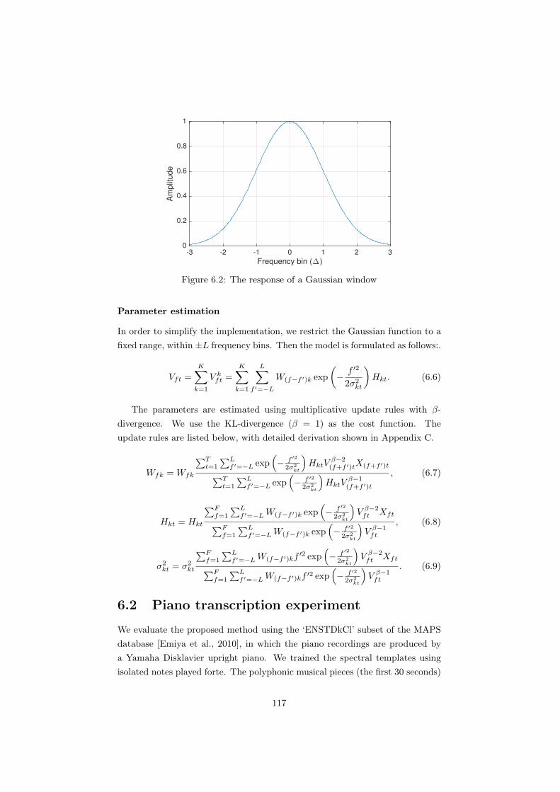
-3 -2 -1 0 1 2 3
Frequency bin (∆)
0
0.2
0.4
0.6
0.8
1
Am
plit
ud
e
Figure 6.2: The response of a Gaussian window
Parameter estimation
In order to simplify the implementation, we restrict the Gaussian function to a
fixed range, within ±L frequency bins. Then the model is formulated as follows:.
Vft =KX
k=1
V kft =
KX
k=1
LX
f 0=�L
W(f�f 0)k exp
✓�
f 02
2�2kt
◆Hkt. (6.6)
The parameters are estimated using multiplicative update rules with �-
divergence. We use the KL-divergence (� = 1) as the cost function. The
update rules are listed below, with detailed derivation shown in Appendix C.
Wfk = Wfk
PTt=1
PLf 0=�L exp
⇣�
f 02
2�2kt
⌘HktV
��2(f+f 0)tX(f+f 0)t
PTt=1
PLf 0=�L exp
⇣�
f 02
2�2kt
⌘HktV
��1(f+f 0)t
, (6.7)
Hkt = Hkt
PFf=1
PLf 0=�L W(f�f 0)k exp
⇣�
f 02
2�2kt
⌘V ��2ft Xft
PFf=1
PLf 0=�L W(f�f 0)k exp
⇣�
f 02
2�2kt
⌘V ��1ft
, (6.8)
�2kt = �2
kt
PFf=1
PLf 0=�L W(f�f 0)kf
02 exp⇣�
f 02
2�2kt
⌘V ��2ft Xft
PFf=1
PLf 0=�L W(f�f 0)kf 02 exp
⇣�
f 02
2�2kt
⌘V ��1ft
. (6.9)
6.2 Piano transcription experiment
We evaluate the proposed method using the ‘ENSTDkCl’ subset of the MAPS
database [Emiya et al., 2010], in which the piano recordings are produced by
a Yamaha Disklavier upright piano. We trained the spectral templates using
isolated notes played forte. The polyphonic musical pieces (the first 30 seconds)
117

are then transcribed with the trained templates.
6.2.1 Pre-processing
Computing STFT
The sample rate of the audio is fs = 44100Hz. To compute the STFT, each
frame is weighted by a Gaussian window covering 4096 samples with a standard
deviation of N = 4096/6 samples. In the time domain, the standard deviation
of the window function is � = N/fs. The hop size is 882 samples. In order to
locate the partial frequencies at the frequency bins, we need a high frequency
resolution. Hence, we perform a 4-fold zero padding before computing the spec-
trum using a discrete Fourier transform (DFT).
The theoretical value of the spectral width
The Fourier transform of the window function g�1(t) = 1p
2⇡�21
e�t2/(2�21) with
standard deviation of �1 is given by
G(f) = F [g�1 ](f) = e�2⇡2�21f
2
. (6.10)
If we set the variance of G(f) to �22 , then e�f2/(2�2
2) = e�2⇡2�21f
2
. So we can
derive that �2 = 12⇡�1
. We know from the previous section that �1 = N/fs.
Then the standard deviation (spectral width) is �2 = fs2⇡N . The frequency
resolution is the ratio of the sample rate fs and the size of the DFT n↵t. We
conclude that the spectral width covers n↵t
2⇡N frequency bins. When we compute
the STFT, n↵t = 16384 and N = 4096/6. So the theoretical value of spectral
width is � = 3.82 frequency bins.
6.2.2 Template training
We train spectral templates on isolated notes in forte from the ‘ENSTDkCl’
subset [Emiya et al., 2010]. For each pitch, we update the spectral template,
activations and spectral widths via Equations 6.7, 6.8 and 6.9 with K = 1 for 30
iterations. The range of the Gaussian response is set to be within ±30 frequency
bins (L = 30).
Initialisation
In order to enforce a harmonic-comb shape for templates, we initialise the tem-
plates with the peaks of the mean spectrum. For each pitch, we first normalise
the spectrum of each frame to a maximum of 1, and compute the average of the
118

normalised spectra. Then we detect peaks of the average normalised spectrum
and use them as the initialisation of the spectral basis.
The activations are randomly initialised and the spectral widths are ini-
tialised with the theoretical value � = 3.82.
Trained examples
There are four examples of tones of di↵erent pitches shown in Figure 6.3. We find
several noticeable characteristics of the spectral width. (1) The spectral width
is large around the onset, and is smaller and remains stable for the remaining
duration of the note, as shown in Figure 6.3(a–c). (2) We can observe a small
peak in the spectral width at the o↵set, as shown in Figure 6.3(b). (3) When the
activation is small, the spectral width is ambiguous. The first case happens in
frames before the onset and after the o↵set of a note, where the spectral width
is theoretically undefined, hence expectedly noisy. The second case happens
within the duration of the note with low amplitude. This usually occurs on
high pitches. For example, as shown in Figure 6.3(d), when the amplitude is
20 dB lower than the maximum amplitude, the spectral width appears noisy.
We show the average spectral widths of all 88 notes in Figure 6.4(a). For
each clip, we discard some of the silent part before the onset to make all notes
start at 0.4 s, and notes end at around 2.5 s. It is clearly shown in Figure 6.4(b)
that the stable average spectral width is above 6 frequency bins, and there is a
major peak near the o↵set. Figure 6.4(c) is the histogram of the spectral width
(below 20 frequency bins), indicating a mode of around 5.5 bins.
6.2.3 Post-processing
After obtaining the activations and spectral widths, we smooth both of them
using a median filter covering 5 time frames. The smoothed activations are
normalised to a maximum of 1 for each piece.
Onset and o↵set detection
Based on the training results, we know that spectral widths are less meaningful
when activations are small. So we first detect active frames by thresholding
on the activations for each pitch. We apply di↵erent thresholds for onsets and
o↵sets. A note starts when the activation is larger than the onset threshold,
and lasts till the activation decreases to below the o↵set threshold.
119
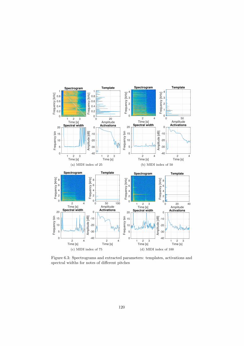
Spectrogram
1 2 3Time [s]
0
0.2
0.4
0.6
0.8
1
Fre
quency
[kH
z]
1 2 3Time [s]
0
5
10
15
20
Fre
quency
bin
Spectral width
0
0.2
0.4
0.6
0.8
1F
requency
[kH
z]
0 20Amplitude
Template
1 2 3Time [s]
-40
-30
-20
-10
0
Am
plit
ude [dB
]
Activations
(a) MIDI index of 25
Spectrogram
2 4Time [s]
0
1
2
3
4
Fre
quency
[kH
z]
2 4Time [s]
0
5
10
15
20F
requency
bin
Spectral width
0
1
2
3
4
Fre
quency
[kH
z]
0 50Amplitude
Template
2 4Time [s]
-40
-30
-20
-10
0
Am
plit
ude [dB
]
Activations
(b) MIDI index of 50
Spectrogram
2 4Time [s]
0
2
4
6
8
Fre
quency
[kH
z]
2 4Time [s]
0
5
10
15
20
Fre
quency
bin
Spectral width
0
2
4
6
8
Fre
quency
[kH
z]
0 50 100Amplitude
Template
2 4Time [s]
-40
-30
-20
-10
0
Am
plit
ude [dB
]
Activations
(c) MIDI index of 75
Spectrogram
1 2 3Time [s]
0
2
4
6
8
Fre
qu
en
cy [
kHz]
1 2 3Time [s]
0
5
10
15
20
Fre
qu
en
cy b
in
Spectral width
0
2
4
6
8
Fre
qu
en
cy [
kHz]
0 20 40Amplitude
Template
1 2 3Time [s]
-40
-30
-20
-10
0
Am
plit
ud
e [
dB
]
Activations
(d) MIDI index of 100
Figure 6.3: Spectrograms and extracted parameters: templates, activations andspectral widths for notes of di↵erent pitches
120

1 2 3 4Time (s)
0
20
40
60
80
100
120
Spect
ral w
idth
(a) The average spectral widths over allpitches
1 2 3 4Time (s)
0
2
4
6
8
10
12
14
16
18
20
Spect
ral w
idth
(b) The average spectral widths (below 20frequency bins)
2 4 6 8 10 12 14 16 18 20Spectral width
0
500
1000
1500
2000
2500
3000
3500
(c) The histogram of spectral widths (below 20 frequency bins)
Figure 6.4: Trained spectral widths.
121
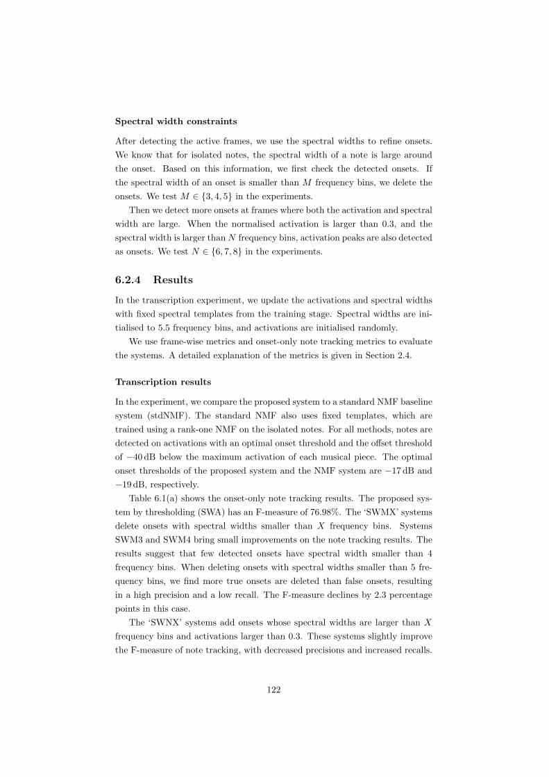
Spectral width constraints
After detecting the active frames, we use the spectral widths to refine onsets.
We know that for isolated notes, the spectral width of a note is large around
the onset. Based on this information, we first check the detected onsets. If
the spectral width of an onset is smaller than M frequency bins, we delete the
onsets. We test M 2 {3, 4, 5} in the experiments.
Then we detect more onsets at frames where both the activation and spectral
width are large. When the normalised activation is larger than 0.3, and the
spectral width is larger thanN frequency bins, activation peaks are also detected
as onsets. We test N 2 {6, 7, 8} in the experiments.
6.2.4 Results
In the transcription experiment, we update the activations and spectral widths
with fixed spectral templates from the training stage. Spectral widths are ini-
tialised to 5.5 frequency bins, and activations are initialised randomly.
We use frame-wise metrics and onset-only note tracking metrics to evaluate
the systems. A detailed explanation of the metrics is given in Section 2.4.
Transcription results
In the experiment, we compare the proposed system to a standard NMF baseline
system (stdNMF). The standard NMF also uses fixed templates, which are
trained using a rank-one NMF on the isolated notes. For all methods, notes are
detected on activations with an optimal onset threshold and the o↵set threshold
of �40 dB below the maximum activation of each musical piece. The optimal
onset thresholds of the proposed system and the NMF system are �17 dB and
�19 dB, respectively.
Table 6.1(a) shows the onset-only note tracking results. The proposed sys-
tem by thresholding (SWA) has an F-measure of 76.98%. The ‘SWMX’ systems
delete onsets with spectral widths smaller than X frequency bins. Systems
SWM3 and SWM4 bring small improvements on the note tracking results. The
results suggest that few detected onsets have spectral width smaller than 4
frequency bins. When deleting onsets with spectral widths smaller than 5 fre-
quency bins, we find more true onsets are deleted than false onsets, resulting
in a high precision and a low recall. The F-measure declines by 2.3 percentage
points in this case.
The ‘SWNX’ systems add onsets whose spectral widths are larger than X
frequency bins and activations larger than 0.3. These systems slightly improve
the F-measure of note tracking, with decreased precisions and increased recalls.
122

Table 6.1: Comparison of the proposed systems with a standard NMF
(a) Note tracking results (onset-only)
method Pon Ron Fon Aon
SWA 80.29 74.89 76.98 63.73SWM3 80.30 74.89 76.99 63.73SWM4 80.94 74.44 77.08 63.87SWM5 84.85 67.41 74.69 61.02SWN6 79.16 76.90 77.48 64.28SWN7 80.14 75.47 77.24 64.05SWN8 80.26 75.22 77.15 63.94stdNMF 78.70 76.73 77.22 64.07
(b) Frame-wise results
method Pf Rf Ff Af
SWA 79.20 79.60 78.36 64.83stdNMF 79.32 79.46 78.35 64.79
When the constraint on spectral width becomes larger, the di↵erence from the
SWA system is smaller, because the number of newly-detected onsets decreases
with the increasing spectral width.
The F-measure of the standard NMF is 77.22%. There are no significant dif-
ferences between the proposed systems and the NMF system. Only the proposed
system of SWN6 has a slightly better F-measure than that of stdNMF.
The frame-wise results are listed in Table 6.1(b). Because refining onsets
using spectral widths usually does not change the frame-wise results, we only
show results of the proposed ‘SWA’ system. The frame-wise results of the
proposed system and the NMF system are similar to each other, with F-measures
of 78.4%.
The results show that refining onsets using spectral widths barely brings im-
provements in transcription performance, and there are no significant di↵erences
between the proposed methods and the standard NMF.
Spectral width distributions
In order to find more sophisticated methods to deal with spectral widths, we
analyse their statistical characteristics. Figure 6.5 shows the distribution of
spectral widths at the onsets for di↵erent pitches. We find that not all onsets
have large spectral widths. The median spectral widths of most low-pitch notes
are below 6 frequency bins at the onsets. The value increases for notes with
123

higher pitch. We suppose that it is related to the frequency interval between
partials. The adjacent partials are overlapped when the spectral width is larger
than a half of the fundamental frequency (frequency interval). Then the spectral
widths of the onsets are limited by the fundamental frequency. Note that the
observation of the spectral widths at onsets in training stage is di↵erent from
that in the transcription experiment. Because in the training stage we perform a
rank-one NMF, the percussive onset can only be represented by the note. Then
it usually has a large onset spectral width. In the transcription experiment,
the spread spectral distribution at the onset can by explained by other notes,
and the spectral width is influenced more by the adjacent frequency bins of the
partials.
For each pitch, the spectral widths also vary, depending on the number of
notes played at the moment. If there is only one note played, the spectral
width is large at the onset. If there are several notes played simultaneously,
the spectral width of one note can be small because the spread energy may be
represented by other notes.
This explains why we can not improve the results by simply deleting onsets
with small spectral widths. In the future, we can try to extend this model in
a CQT TF representation, which has constant spaces between partials for all
pitches. However, we would need to deal with anther problem of the model in
the CQT: the spectral widths of partials of a note change with frequency.
Figure 6.6 shows the distribution of spectral widths in the decay parts. In
the middle pitch range, the median value of the spectral widths is around 5
frequency bins. Notes in the low pitch range tend to have smaller spectral
widths, and the spectral width is less predictable for pitches above MIDI index
of 80. Even for notes of the same pitch, the range of the spectral width is large.
First we know that the spectral width is closely related to the activation. When
the activation is small, the spectral width is small too. Secondly the spectral
width is easily influenced by notes of other pitches. For example, in Figure 6.7
the note of pitch D4 (MIDI index 62) starts at around 0.5 s and lasts till the end
of the clip. When the note activations are relatively large (before 5 s as shown
in Figure 6.7(b)), the spectral widths in most frames are around 5 frequency
bins, as shown in Figure 6.7(a). The false peaks in the spectral width occur
because notes of other pitches start.
We summarise the reasons for slight improvements by adding more onsets
with large activations and spectral widths as follows. First, these onsets are
easy to detect; some of the added onsets have been already detected by thresh-
olding. Secondly, because the spectral width is influenced by the activation and
other notes, there are also false onsets detected along with the true onsets. In
the future, we need to reduce the dependence of the spectral widths on the
124

0 2 4 6 8
10
12
14
16
18
20
Spectral width
26272829303132333435363738394041424344454647484950515253545556575859606162636465666768697071727374757677787980818283848586878889909192939495969899100101102103
Figure 6.5: Box-and-whisker plots of spectral widths (below 20 frequency bins)at onsets, with pitch in MIDI index on the vertical axis.
125

0 2 4 6 8
10
12
14
16
18
20
Spectral width
2627282930313233343536373839404142434445464748495051525354555657585960616263646566676869707172737475767778798081828384858687888990919293949596979899100101102103
Figure 6.6: Box-and-whisker plots of spectral widths (below 20 frequency bins)in decay stages, with pitch in MIDI index on the vertical axis.
126

0 1 2 3 4 5 6Time [s]
0
2
4
6
8
10
12
Spe
ctra
l wid
th
(a) Spectral width of pitch D4 (MIDI index of 62)
0 1 2 3 4 5 6Time [s]
0
0.2
0.4
0.6
0.8
1
Am
ptit
ude
(b) Activation of pitch D4 (MIDI index 62)
Figure 6.7: An example of the spectral width and activation for one pitch duringthe first 6 seconds of the piece ‘alb se2’.
activations and impose constraints on spectral widths, such as continuity.
6.3 Conclusions and future work
In this chapter we study the spectral width for piano transcription. We first
model the spectral width of a partial by the standard deviation of the Gaussian
window response. Then we present the spectral basis by the convolution of
a comb-shaped spectral basis and a Gaussian function. So di↵erent spectral
distributions of the attack and decay parts can be modelled by di↵erent spectral
widths. All unknown parameters are estimated in the NMF framework.
In the training stage we find the spectral width is large in the attack part,
and is smaller and remain stable in the decay part. But the spectral width is
related to the activation, which is less meaningful when the activation is small.
In the transcription experiment, we find that the results of proposed systems
are similar to that of a standard NMF system. Refining onsets by the spectral
width shows no significant di↵erences in the transcription performance.
The spectral width distribution at onsets shows that the spectral width is
pitch-dependent at onsets in musical pieces, with a trend that higher pitch
notes have larger spectral widths at onsets. The spectral width distribution
127

in the decay parts shows more than half of the spectral widths are around 5
frequency bins, but there are still large numbers of spectral widths outside the
range.
In this chapter, we have only an exploration on the spectral width. In
the future, in order to e↵ectively use the spectral width information, we first
would like to extend the method in a CQT TF representation, to deal with the
pitch-dependent spectral width for onsets. In addition, the length of the frames
compared to the decay time should be studied in detail to explain the spectral
widths of onsets. Thirdly, we need to decouple the dependence of the spectral
width on the activation. At last, we will experiment with imposing constraints
on spectral widths to reduce the influence by simultaneous notes.
128
Chapter 7
Conclusions and Future
Work
In this thesis, we study piano acoustics for automatically transcribing poly-
phonic music. We focus on features such as the time-varying timbre and decay
amplitudes of piano notes, and model these acoustical features from di↵erent
aspects with the parametric NMF. This chapter first summarises the primary
work of the main chapters, then we show several directions worth future inves-
tigation.
7.1 Conclusions
In Chapter 3, we address the local minimum problem of a PLCA-based tran-
scription method with a deterministic annealing EM algorithm. The EM-based
update rules are modified by introducing a temperature parameter. A more
fine-grained optimisation can be found by gradually decreasing the tempera-
ture. The results show that the proposed method improves the transcription
performance. The optimisation method can also be adapted to the NMF-based
model, because of the similarity between these two matrix factorisation methods.
In Chapter 5, we use a similar annealing process in the proposed NMF-based
model.
In Chapter 4, we study piano decay in real recordings. We first find partials
by modelling their inharmonicity, and then track the decay of the partials. We
focus on three decay patterns with spectral power in dB: linear decay, double
decay and decay with amplitude modulations (beats) according to the theoreti-
cal studies on coupled piano strings [Weinreich, 1977]. We track first 30 partials
below the Nyquist frequency of 88 notes in three dynamic levels. The results
129
verify that partials of higher frequencies decay faster, and the dynamic level has
less impact on the decay pattern.
In Chapter 5, we propose an attack/decay model for piano transcription,
with the spectra of the attack and decay parts represented by two individual
spectral templates for each pitch. This method also models the amplitude en-
velopes for the two parts. The attack envelopes are trained on isolated notes,
and we use the average attack envelope over all pitches. The decay envelope is
parameterised by an exponential decay function, with the decay rate trained for
each isolated note. The two parts are coupled by the note activations, which
means that the decay part always occurs after the corresponding attack part.
We detect onsets on attack activations by peak-picking and track pitch states
by dynamic programming to find o↵sets.
The attack/decay model provides promising transcription results and out-
perform two state-of-the-art methods on the MAPS database [Emiya et al.,
2010]. In the transcription experiments, we compare the fixed sparsity factors
and annealing sparsity factors, based on our studies in Chapter 3. Results in-
dicate that the annealing sparsity factor improves both performance and the
robustness of the proposed model slightly. The exponential decay is a simplifi-
cation of the observed decay patterns in Chapter 4, but it is su�ciently close
to reality to give the observed improvement in transcription results.
We test the proposed method on repeated notes of single pitches. Results
indicate that the assumption of exponential decay causes many false positives
on notes in the low pitch range, due to the beats in the decay. The simplification
of ignoring o↵sets at the first stage works well for long notes, but may cause
false negatives on short notes.
The onset-o↵set note tracking results in Chapter 5 suggest that it is hard
to detect o↵sets on decaying energies. In order to find a more stable indicator
for note tracking, we preliminarily study the spectral widths of piano partials
in Chapter 6. In the proposed model, the time-varying timbre of a piano note
in the attack and decay parts is parameterised by the same spectral basis with
di↵erent spectral widths. The spectral basis consists of peaks at frequencies of
partials. We assume that the spectral width is large at the attack part, but
is smaller and remains constant in the decay part. We represent the spectral
shape of a partial by a Gaussian function. The expected value of the Gaussian
function is the partial frequency and we use the standard deviation � to indicate
the spectral width. With this parametric spectral template, we can estimate
spectral widths directly in the NMF framework.
In the training stage the spectral widths of most isolated notes are in line
with our assumption: large in the attack part, and smaller and stable in the
decay part. But when the activation of the note is small, the spectral width is
130

less predictable, especially for high-pitch notes. In the transcription experiment,
the results of proposed systems are similar to those of a standard NMF system.
No di↵erence in transcription performance is obtained by using the spectral
widths to refine the detected onsets.
In order to find the problems of this preliminary model, we analyse the
spectral distribution in the attack and decay parts in polyphonic music pieces
individually. The spectral width distribution at onsets shows that the spectral
width is pitch-dependent at onsets in musical pieces, with higher pitch notes
having larger spectral widths. The spectral width distribution in the decay
parts shows more than 50% of spectral widths are around 5 frequency bins, but
there are still large numbers of spectral widths outside this range.
The methods presented in this thesis are based on the matrix-factorisation
method. Because the time-varying timbre and decay of energy are not well fit-
ted by this kind of method, we extend the NMF method using cues from piano
acoustics. Based on the proposed methods we can design a combined transcrip-
tion system. Both models in Chapter 5 and 6 present the attack and decay parts
of piano sounds separately. We can use the representation in Chapter 6 for the
attack/decay model in Chapter 5: the attack part is represented by partials
with large spectral widths, and the decay part by partials with small spectral
widths. The method in Chapter 3 addresses the local minimum problem as an
optimisation problem. It could be generalised for parameter estimation in the
NMF framework.
7.2 Further work
Modelling the decay
In the attack/decay model (Chapter 5), we first simplify the note amplitudes to
decay exponentially. Based on the studies in Chapter 4, we know that the decay
is frequency-dependent, with upper partials usually decaying more quickly. We
would like to extend the exponential decay model to be frequency-dependent by
replacing the decay rate by a decay filter. Another simplification of the model
is that the amplitude of a note is assumed to decay till the end of the music
piece, so that we do not need to deal with o↵sets when we formulate the model
in the NMF framework. If we consider the parametric attack and decay parts
as a parametric patch, this simplification means that the parameter patches
are of the same length as the music pieces. In the future, we would like to
extend the model with note-varying durations, which are expected to improve
the transcription performance on piano pieces with many short notes.
131

The idea of decay modelling can also be extended to existing methods. For
example, we find that the unsupervised transcription system [Vincent et al.,
2010] in the comparison experiment of Chapter 5 is a good baseline method.
Each template in this method is a weighted combination of narrow-band spectral
bases. We can extend the system with decay parameters to build an unsuper-
vised system. We can further model each narrow-band spectral basis to decay
at di↵erent rates to build a model which is closer to the real decay of piano
notes.
Modelling spectral widths
In Chapter 6, we present a preliminary study on spectral width. The most
distinguishing problem is that the spectral width is dependent on the note am-
plitude. The spectral width is only interpretable when the corresponding note
amplitude is large enough. We need to decouple the dependence of the spectral
width on the amplitude. Secondly, the spectral widths are fluctuating, and are
easily influenced by simultaneous notes. We expect that this problem could be
lessened by imposing constraints, such as sparsity and continuity, on activations
and spectral widths. In our analysis of the spectral width distribution of the
note onsets, we find that the spectral width of an note onset is related to the
interval between adjacent partials. We would like to extend the method with
a CQT TF representation, to deal with the pitch-dependent spectral widths of
onsets.
Extension to other pianos
We would like to extend the idea of modelling acoustic features of a particular
piano to a general model of an arbitrary piano in the future. The research
questions associated with this direction are: what are the primary di↵erences
between two pianos, and can we share the similar parts but only model the
di↵erences when the training dataset and the test dataset are produced by
di↵erent pianos?
From the concept of the source-filter model, a piano has 88 sources (one for
each pitch) and a filter (the soundboard). Modelling a piano with the source-
filter model is not suitable, as evidenced by our previous work [Cheng et al.,
2014]. For a particular piano, we can train spectral templates on each isolated
note. But for another piano, can we use the same trained templates, but intro-
duce a filter to model the di↵erence between the frequency responses of the two
pianos?
To illustrate the idea, we extended the model for spectral widths (Chapter 6)
with a filter to model the frequency response di↵erence. The filter is param-
132

eterised using the auto-regressive moving average (ARMA) model [Hennequin
et al., 2011a]. We use the templates trained on the subset ENSTDkCl subset
(Disklavier piano) of the MAPS database [Emiya et al., 2010], and employ the
extended model on music pieces in the ENSTDkAm subset (Disklavier piano)
and the AkPnCGdD subset (synthetic piano). The estimated filters are shown
in Figure 7.1. We find that there are fewer high-frequency partials resonated in
the synthetic piano. Although in the preliminary test, we find no di↵erence in
transcription results with and without the filter, we would like to work further
on this direction in the future.
Extension to other instruments
The proposed methods are motivated by piano acoustics. We suppose that they
can be used on instruments with similar acoustical features. The attack/decay
model in Chapter 5 should be apt in struck-string (for example the dulcimer) or
plucked-string instruments (for instance the harpsichord and guitar), because
the sounds produce by these kinds of instruments also have percussive onsets
and then decaying energies. The spectral width model in Chapter 6 is more
general. All harmonic sounds should have stable spectral widths, so we imagine
this model could have application across a large range of instrumental sounds.
133
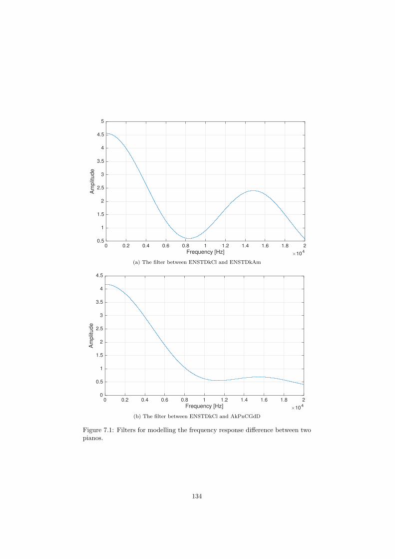
0 0.2 0.4 0.6 0.8 1 1.2 1.4 1.6 1.8 2Frequency [Hz]
×104
0.5
1
1.5
2
2.5
3
3.5
4
4.5
5
Am
plit
ude
(a) The filter between ENSTDkCl and ENSTDkAm
0 0.2 0.4 0.6 0.8 1 1.2 1.4 1.6 1.8 2Frequency [Hz]
×104
0
0.5
1
1.5
2
2.5
3
3.5
4
4.5
Am
plit
ude
(b) The filter between ENSTDkCl and AkPnCGdD
Figure 7.1: Filters for modelling the frequency response di↵erence between twopianos.
134

Appendix A
Beating in the dB scale
In [Weinreich, 1977], the beating of two strings is represented by Equation (20),
which is written as follows:
R(t) = exp(�2⌘t)⇥ (µ cosµt� ⌘sinµt)2/µ2, (A.1)
where the beating frequency is 2µ and the decay rate is 2⌘. We know that
(µ cosµt� ⌘sinµt)2 = (µ2 + ⌘2) cos(µt+ ')2, (A.2)
where ' = arg tan(⌘/µ). Then the equation can be rewritten as:
R(t) = exp(�2⌘t)⇥µ2 + ⌘2
µ2⇥ cos(µt+ ')2. (A.3)
We write the equation in the dB scale for curve fitting:
RdB(t) = 20 log10(exp(�2⌘t)⇥µ2 + ⌘2
µ2⇥ cos(µt+ ')2)
= 20 log10(exp(�2⌘t)) + 20 log10(µ2 + ⌘2
µ2) + 20 log10(cos(µt+ ')2))
= �40⌘ log10(e)⇥ t+ 20 log10(µ2 + ⌘2
µ2) + 40 log10(| cos(µt+ ')|).
(A.4)
We replace the parameters with a = �40⌘ log10(e) and b = 20 log10(µ2+⌘2
µ2 ),
then the equation can be written as:
RdB(t) = at+ b+ 40 log10(| cos(µt+ ')|). (A.5)
135

This equation represents the purely resistive coupling of the two strings. The
amplitude of the beating will change if this is not the case [Weinreich, 1977].
So we replace 40 by A, which is a parameter to estimate. We also replace µ by
f to intuitively represent the frequency, and a small value " is added to avoid
taking the log of 0. Then the final equation is written as:
RdB(t) = at+ b+A log10(| cos(ft+ ')|+ "), (A.6)
which is the form we use in Equation 4.5.
136

Appendix B
Derivations for the
attack/decay model
As described in Chapter 5, the proposed model is formulated as follows:
Vft =KX
k=1
W afkH
akt +
KX
k=1
W dfkH
dkt
=KX
k=1
W afk
t+TaX
⌧=t�Ta
Hk⌧P (t� ⌧) +KX
k=1
W dfk
tX
⌧=1
Hk⌧e�(t�⌧)↵k ,
(B.1)
where V is the reconstruction of the spectrogram, f 2 [1, F ] is the frequency
bin, and t 2 [1, T ] indicates the time frame. Wa and Wd are the percussive and
harmonic templates, and k 2 [1,K] is the pitch index. Ha are attack activations,
generated by the convolution of note activations H and the attack envelope P.
Hd are decay activations and ↵k are decay factors. In Chapter 5, we assume
the harmonic phase starts at the onset time, then the maximum value of the
trained attack envelope occurs at one frame before the onset.
We add a parameter Td to control the start time of the harmonic part. Decay
activations are therefore represented by:
Hdkt =
t�TdX
⌧=1
Hk⌧e�(t�(⌧+Td))↵k . (B.2)
This indicates that the harmonic part starts at Td frames after the onset. When
the music piece is too long, we also need a parameter as the maximal duration
Tmax . Then in the convolution, max(1, t � Tmax ) ⌧ t � Td. We set tm =
137

max(1, t� Tmax ), then decay activations are represented as:
Hdkt =
t�TdX
⌧=tm
Hk⌧e�(t�(⌧+Td))↵k . (B.3)
Then the complete proposed model is formulated as follows:
Vft =KX
k=1
W afk
t+TaX
⌧=t�Ta
Hk⌧P (t� ⌧) +KX
k=1
W dfk
t�TdX
⌧=tm
Hk⌧e�(t�(⌧+Td))↵k . (B.4)
In Chapter 5, we use a simplified model with Td = 0 and Tmax = T , then tm = 1.
Here we work on the complete model.
The parameters are estimated by minimising the distance between the spec-
trogram and the reconstruction by multiplicative update rules [Lee and Seung,
2000]. The derivative of the cost function with respect to (w.r.t.) ✓ is written
as a di↵erence of two non-negative functions:
r✓D(✓) = r+✓ D(✓)�r�
✓ D(✓). (B.5)
The multiplicative algorithm is given by ✓ ✓.r�✓ D(✓)./r+
✓ D(✓). We minimise
the �-divergence between the spectrogram X and the reconstruction V, with
the �-divergence given as follows [Fevotte, 2011]:
d�(x|y) =
8>>><
>>>:
1�(��1) (x
� + (� � 1)y� � �xy��1) � 2 R \ {0, 1},
xlog xy � x+ y � = 1,
xy � log x
y � 1 � = 0.
(B.6)
The derivative of the �-divergence w.r.t. ✓ is given by [Fevotte, 2011]:
r✓D(✓) = r✓d�(X|V (✓))
= (V (✓)��1�XV (✓)��2)r✓V (✓).
(B.7)
The update rule is [Fevotte, 2011]
✓ ✓.V (✓)��1
r
�✓ V (✓) +XV (✓)��2
r
+✓ V (✓)
XV (✓)��2r
�✓ V (✓) + V (✓)��1
r
+✓ V (✓)
. (B.8)
The derivative of Vft w.r.t. W afk is
rWafkVft = r
+Wa
fkVft =
t+TaX
⌧=t�Ta
Hk⌧P (t� ⌧), (B.9)
138

then the update rule of W afk is
W afk W a
fk
PTt=1
Pt+Ta
⌧=t�TaHk⌧P (t� ⌧)(V ��2
ft Xft)PT
t=1
Pt+Ta
⌧=t�TaHk⌧P (t� ⌧)V ��1
ft
. (B.10)
The derivative of Vft w.r.t. W dfk is
rWdfkVft = r
+Wd
fkVft =
t�TdX
⌧=tm
Hk⌧e�(t�(⌧+Td))↵k , (B.11)
then the update rule of W dfk is
W dfk W d
fk
PTt=1
Pt�Td
⌧=tmHk⌧e
�(t�(⌧+Td))↵k(V ��2ft Xft)
PTt=1
Pt�Td
⌧=tmHk⌧e�(t�(⌧+Td))↵kV ��1
ft
. (B.12)
The derivative of Vft w.r.t. ↵k is
r↵kVft = r�↵k
Vft = W dfk
t�TdX
⌧=tm
Hk⌧e�(t�(⌧+Td))↵k(t� (⌧ + Td)), (B.13)
then the update rule of ↵k is
↵k ↵k
PFf=1
PTt=1 W
dfk
Pt�Td
⌧=tmHk⌧e
�(t�(⌧+Td))↵k(t� (⌧ + Td))V��1ftPF
f=1
PTt=1 W
dfk
Pt�Td
⌧=tmHk⌧e�(t�(⌧+Td))↵k(t� (⌧ + Td))(V
��2ft Xft)
.
(B.14)
We set x = t� ⌧ , then the reconstruction is given by replacing t with ⌧ + x
Vf(⌧+x) =KX
k=1
W afk
t+TaX
⌧=t�Ta
Hk⌧P (x) +KX
k=1
W dfk
t�TdX
⌧=tm
Hk⌧e�(x�Td)↵k (B.15)
We derive the ranges of the two summations with respect to x. In the first one
t� Ta ⌧ t+ Ta ) t� Ta t� x t+ Ta, so �Ta x Ta. In the second
one the upper limit is ⌧ t� Td ) t� x t� Td, so x � Td. The lower limit
is ⌧ � max(1, t � Tmax ). If t � Tmax > 1 ) t � x � t � Tmax , so x Tmax . If
t � Tmax 1 ) ⌧ � 1, which gives no restriction to the range of x. Then the
range is determined by the following restriction: t Tmax+1) ⌧+x Tmax+1,
so 1 ⌧ Tmax +1�x) x Tmax . Combining these two conditions, we have
Td x Tmax . With these two ranges, the reconstruction is rewritten as
Vf(⌧+x) =KX
k=1
W afk
TaX
x=�Ta
Hk⌧P (x) +KX
k=1
W dfk
TmaxX
x=Td
Hk⌧e�(x�Td)↵k (B.16)
139

We replace ⌧ with t to obtain more consistent equations:
Vf(t+x) =KX
k=1
W afk
TaX
x=�Ta
HktP (x) +KX
k=1
W dfk
TmaxX
x=Td
Hkte�(x�Td)↵k (B.17)
The derivative of Vft w.r.t. Hkt is
rHktVf(t+x) = r+Hkt
Vf(t+x) = W afk
TaX
x=�Ta
P (x) +W dfk
TmaxX
x=Td
e�(x�Td)↵k , (B.18)
then the update rule of Hkt is
Hkt Hkt
PFf=1(W
afk
PTa
x=�TaP (x) +W d
fk
PTmax
x=Tde�(x�Td)↵k)(V ��2
f(t+x)Xf(t+x))PF
f=1(Wafk
PTa
x=�TaP (x) +W d
fk
PTmax
x=Tde�(x�Td)↵k)V ��1
f(t+x)
.
(B.19)
The derivative of Vft w.r.t. P (x) with Equation B.17 is :
rP (x)Vf(t+x) = r+P (x)Vf(t+x) =
KX
k=1
W afkHkt, (B.20)
then the update rule of P (x) is
P (x) P (x)
PFf=1
PTt=1
PKk=1 W
afkHkt(V
��2f(t+x)Xf(t+x))
PFf=1
PTt=1
PKk=1 W
afkHktV
��1f(t+x)
. (B.21)
140

Appendix C
Derivations for modelling
spectral widths
In Chapter 6, we propose a parametric NMF model with time-varying spectral
widths for each pitch. The Gaussian function representing the spectral shape
for partials of pitch k at the tth frame is given by:
G(f |�kt) = exp
✓�
f2
2�2kt
◆,�3�kt f 3�kt (C.1)
where �kt is the time-varying standard deviation (spectral width), and the Gaus-
sian function has a maximum value of 1 and is restricted in a range of ±3�kt.
The spectrum of pitch k in the f th frequency bin and the tth frame V kft is
modelled by the convolution of the spectral basis wk and the Gaussian window
response G(f |�kt), scaled by the current activation Hkt:
V kft = [wk ⇤G(f |�kt)]fHkt =
3�ktX
f 0=�3�kt
W(f�f 0)k exp
✓�
f 02
2�2kt
◆Hkt, (C.2)
where the spectral basis (wk 2 RF ) only has peaks at the partial frequencies.
The whole spectrum is formulated as a sum over all pitches:
Vft =KX
k=1
V kft =
KX
k=1
3�ktX
f 0=�3�kt
W(f�f 0)k exp
✓�
f 02
2�2kt
◆Hkt. (C.3)
141

Parameter estimation
In order to simplify the implementation, we restrict the Gaussian function in a
fixed range, within ±L frequency bins. Then the model is formulated as follows:.
Vft =KX
k=1
V kft =
KX
k=1
LX
f 0=�L
W(f�f 0)k exp
✓�
f 02
2�2kt
◆Hkt. (C.4)
The parameters are estimated using multiplicative update rules with �-
divergence as in Appendix B. The derivative of the �-divergence w.r.t. ✓ is
given by the subtraction of two non-negative parts:
r✓D(✓) = (V(✓)��1�XV(✓)��2)r✓V(✓), (C.5)
where X the observed spectrogram. The update rule for ✓ is
✓ ✓.V(✓)��1
r
�✓ V(✓) +XV(✓)��2
r
+✓ V(✓)
XV(✓)��2r
�✓ V(✓) +V(✓)��1
r
+✓ V(✓)
. (C.6)
We first derive the update rule for Wfk as follows:
V(f+f 0)t =KX
k=1
LX
f 0=�L
Wfk exp(�f 02
2�2kt
)Hkt, (C.7)
@V(f+f 0)t
@Wfk=
LX
f 0=�L
exp(�f 02
2�2kt
)Hkt. (C.8)
Then the update rule for Wfk is:
Wfk Wfk
PTt=1
PLf 0=�L exp(� f 02
2�2kt)HktV
��2(f+f 0)tX(f+f 0)t
PTt=1
PLf 0=�L exp(� f 02
2�2kt)HktV
��1(f+f 0)t
. (C.9)
The derivative of the reconstruction Vft w.r.t. Hkt is given by:
@Vft
@Hkt=
LX
f 0=�L
W(f�f 0)k exp(�f 02
2�2kt
), (C.10)
so the update rule for Hkt is:
Hkt Hkt
PFf=1
PLf 0=�L W(f�f 0)k exp(�
f 02
2�2kt)V ��2
ft Xft
PFf=1
PLf 0=�L W(f�f 0)k exp(�
f 02
2�2kt)V ��1
ft
. (C.11)
142
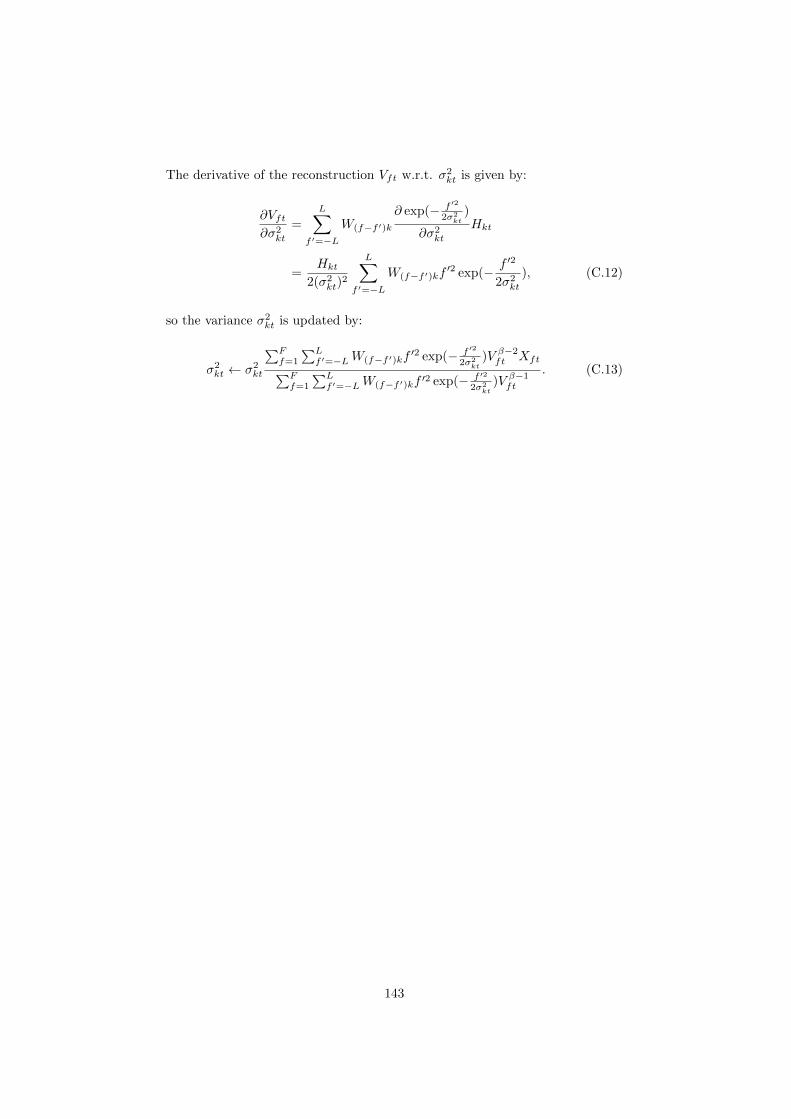
The derivative of the reconstruction Vft w.r.t. �2kt is given by:
@Vft
@�2kt
=LX
f 0=�L
W(f�f 0)k
@ exp(� f 02
2�2kt)
@�2kt
Hkt
=Hkt
2(�2kt)
2
LX
f 0=�L
W(f�f 0)kf02 exp(�
f 02
2�2kt
), (C.12)
so the variance �2kt is updated by:
�2kt �2
kt
PFf=1
PLf 0=�L W(f�f 0)kf
02 exp(� f 02
2�2kt)V ��2
ft Xft
PFf=1
PLf 0=�L W(f�f 0)kf 02 exp(� f 02
2�2kt)V ��1
ft
. (C.13)
143
Bibliography
S. A. Abdallah and M. D. Plumbley. Polyphonic music transcription by non-
negative sparse coding of power spectra. In 5th International Conference on
Music Information Retrieval (ISMIR), pages 318–325, 2004.
M. Aramaki, J. Bensa, L. Daudet, P. Guillemain, and R. Kronland-Martinet.
Resynthesis of coupled piano string vibrations based on physical modeling.
Journal of New Music Research, 30(3):213–226, 2001.
B. Bank. Physics-based sound synthesis of the piano. Master’s thesis, Budapest
University of Technology and Economics, Hungary, 2000.
B. Bank. Accurate and e�cient modeling of beating and two-stage decay for
string instrument synthesis. In MOSART Workshop on Current Research
Directions in Computer Music, pages 134–137, 2001.
M. Bay, A. F. Ehmann, and J. S. Downie. Evaluation of multiple-F0 estimation
and tracking systems. In 10th International Society for Music Information
Retrieval Conference (ISMIR), pages 315–320, 2009.
M. Bay, A. F. Ehmann, J. W. Beauchamp, P. Smaragdis, and J. S. Downie. Sec-
ond fiddle is important too: Pitch tracking individual voices in polyphonic
music. In 13th International Society for Music Information Retrieval Confer-
ence (ISMIR), pages 319–324, 2012.
J. M. Becker, C. Sohn, and C. Rohlfing. NMF with spectral and temporal
continuity criteria for monaural sound source separation. In European Signal
Processing Conference (EUSIPCO), pages 316 – 320, 2014.
E. Benetos. Automatic transcription of polyphonic music exploiting temporal
evolution. PhD thesis, Queen Mary University of London, 2012.
E. Benetos and S. Dixon. A shift-invariant latent variable model for automatic
music transcription. Computer Music Journal, 36(4):81–94, 2012a.
144
E. Benetos and S. Dixon. Multiple-F0 estimation and note tracking for MIREX
2012 using a shift-invariant latent variable model. In Music Information Re-
trieval Evaluation eXchange (MIREX), 2012b.
E. Benetos and S. Dixon. Multiple-instrument polyphonic music transcription
using a temporally constrained shift-invariant model. The Journal of the
Acoustical Society of America, 133(3):1727–1741, 2013.
E. Benetos and T. Weyde. An e�cient temporally-constrained probabilistic
model for multiple-instrument music transcription. In 16th International So-
ciety for Music Information Retrieval Conference (ISMIR), pages 701–707,
2015a.
E. Benetos and T. Weyde. Multiple-F0 estimation and note tracking for MIREX
2015 using a sound state-based spectrogram factorization model. In Music
Information Retrieval Evaluation eXchange (MIREX), 2015b.
E. Benetos, S. Cherla, and T. Weyde. An e�cient shift-invariant model for
polyphonic music transcription. In 6th International Workshop on Machine
Learning and Music, 2013a.
E. Benetos, S. Dixon, D. Giannoulis, H. Kirchho↵, and A. Klapuri. Automatic
music transcription: challenges and future directions. Journal of Intelligent
Information Systems, 41(3):407–434, 2013b.
E. Benetos, R. Badeau, T. Weyde, and G. Richard. Template adaptation for im-
proving automatic music transcription. In 15th International Society for Mu-
sic Information Retrieval Conference (ISMIR), pages 175–180, Taipei, 2014.
J. Bensa, S. Bilbao, R. Kronland-Martinet, and J. O. Smith. The simulation of
piano string vibration: From physical models to finite di↵erence schemes and
digital waveguides. The Journal of the Acoustical Society of America, 114(2):
1095–1107, 2003.
T. Berg-Kirkpatrick, J. Andreas, and D. Klein. Unsupervised transcription of
piano music. In Advances in Neural Information Processing Systems 27, pages
1538–1546, 2014.
N. Bertin, R. Badeau, and E. Vincent. Fast Bayesian NMF algorithms enforcing
harmonicity and temporal continuity in polyphonic music transcription. In
IEEE Workshop on Applications of Signal Processing to Audio and Acoustics
(WASPAA), pages 29–32, 2009a.
N. Bertin, C. Fevotte, and R. Badeau. A tempering approach for Itakura-Saito
non-negative matrix factorization. With application to music transcription. In
145
IEEE International Conference on Acoustics, Speech, and Signal Processing
(ICASSP), pages 1545–1548, 2009b.
N. Bertin, R. Badeau, and E. Vincent. Enforcing harmonicity and smoothness in
Bayesian non-negative matrix factorization applied to polyphonic music tran-
scription. IEEE Transactions on Acoustics, Speech, and Signal Processing, 18
(3):538–549, 2010.
E.D. Blackham. The physics of the piano. Scientific American, 213(6), 1965.
S. Bock and M. Schedl. Polyphonic piano note transcription with recurrent
neural networks. In IEEE International Conference on Acoustics, Speech and
Signal Processing (ICASSP), pages 121–124, 2012.
S. Bock and G. Widmer. Local group delay based vibrato and tremolo suppres-
sion for onset detection. In 14th International Society for Music Information
Retrieval Conference (ISMIR), pages 589–594, November 2013.
J. C. Brown. Calculation of a constant Q spectral transform. The Journal of
the Acoustical Society of America, 89(1):425434, 1991.
J. J. Burred. The acoustics of the Piano. PhD thesis, Professional Conservatory
of Music Arturo Soria, 2004.
B. Capleton. False beats in coupled piano string unisons. The Journal of the
Acoustical Society of America, 115(2):885–892, 2004.
A. T. Cemgil. Bayesian inference for nonnegative matrix factorisation models.
Computational Intelligence and Neuroscience, 2009.
A. Chaigne and J. Kergomard. Acoustics of Musical Instruments. Springer-
Verlag New York, 2016.
Z. Chen, G. Grindlay, and D. P. W. Ellis. Transcribing multi-instrument poly-
phonic music with transformed eigeninstrument whole-note templates. In
Music Information Retrieval Evaluation eXchange (MIREX), 2012.
T. Cheng, S. Dixon, and M. Mauch. A deterministic annealing EM algorithm
for automatic music transcription. In 14th International Society for Music
Information Retrieval Conference (ISMIR), pages 475–480, 2013.
T. Cheng, S. Dixon, and M. Mauch. A comparison of extended source-filter mod-
els for musical signal reconstruction. In International Conference on Digital
Audio E↵ects (DAFx), pages 203–209, 2014.
146
T. Cheng, S. Dixon, and M. Mauch. Modelling the decay of piano sounds. In
IEEE International Conference on Acoustics, Speech and Signal Processing
(ICASSP), pages 594–598, 2015a.
T. Cheng, S. Dixon, and M. Mauch. Improving piano note tracking by HMM
smoothing. In European Signal Processing Conference (EUSIPCO), pages
2009–2013, 2015b.
M. Christensen and A. Jakobsson. Multi-Pitch Estimation. Morgan & Claypool,
2009.
A. Cogliati and Z. Duan. Piano music transcription modeling note temporal
evolution. In IEEE International Conference on Acoustics, Speech and Signal
Processing (ICASSP), pages 429–433, 2015.
A. Cont. Realtime multiple pitch observation using sparse non-negative con-
straints. In 7th International Conference on Music Information Retrieval
(ISMIR), pages 206–211, 2006.
A. Cont, S. Dubnov, and D. Wessel. Realtime multiple-pitch and multiple-
instrument recognition for music signals using sparse non-negative con-
straints. In International Conference on Digital Audio E↵ects (DAFx), pages
85–92, 2007.
A. de Cheveigne. Cancellation model of pitch perception. The Journal of the
Acoustical Society of America, 103(3):1261–1271, 1998.
A. de Cheveigne. Multiple f0 estimation. In Computational Auditory Scene
Analysis, Algorithms and Applications. IEEE Press/Wiley, New York, 2006.
A. de Cheveigne and H. Kawahara. YIN, a fundamental frequency estimator
for speech and music. The Journal of the Acoustical Society of America, 111
(4):1917–1930, 2002.
A. Dessein, A. Cont, and G. Lemaitre. Real-time polyphonic music transcription
with non-negative matrix factorization and beta-divergence. In 11th Inter-
national Society for Music Information Retrieval Conference (ISMIR), pages
489–494, 2010.
S. Dixon. On the computer recognition of solo piano music. In Australasian
Computer Music Conference, pages 31–37, 2000.
K. Dressler. Pitch estimation by the pair-wise evaluation of spectral peaks.
In Audio Engineering Society Conference: 42nd International Conference on
Semantic Audio, pages 278–290, 2011.
147

Z. Duan and D. Temperley. Note-level music transcription by maximum likeli-
hood sampling. In 15th International Society for Music Information Retrieval
Conference (ISMIR), pages 181–186, 2014.
Z. Duan, B. Pardo, and C. Zhang. Multiple fundamental frequency estimation
by modeling spectral peaks and non-peak regions. IEEE Transactions on
Audio, Speech, and Language Processing, 18(8):2121–2133, 2010.
N. Q. K. Duong, E. Vincent, and R. Gribonval. Under-determined reverber-
ant audio source separation using local observed covariance and auditory-
motivated time-frequency representation. In 9th International Conference on
Latent Variable Analysis and Signal Separation, pages 73–80, 2010.
J. Eggert and E. Korner. Sparse coding and NMF. In IEEE International Joint
Conference on Neural Networks, pages 2529–2533, 2004.
V. Emiya, B. David, and R. Badeau. A parametric method for pitch estimation
of piano tones. In IEEE International Conference on Acoustics, Speech and
Signal Processing(ICASSP), volume 1, pages 249–252, 2007.
V. Emiya, R. Badeau, and B. David. Multipitch estimation of piano sounds
using a new probabilistic spectral smoothness principle. IEEE Transactions
on Audio, Speech, and Language Processing, 18(6):1643–1654, 2010.
S. Ewert, M. D. Plumbley, and M. Sandler. A dynamic programming variant
of non-negative matrix deconvolution for the transcription of struck string
instruments. In IEEE International Conference on Acoustics, Speech and
Signal Processing (ICASSP), pages 569–573, 2015.
C. Fevotte. Majorization-Minimisation algorithm for smooth Itakuro-Saito non-
negative matrix factorization. In IEEE International Conference on Acous-
tics, Speech and Signal Processing (ICASSP), pages 1980–1983, 2011.
C. Fevotte, N. Bertin, and J.-L. Durrieu. Nonnegative matrix factorization with
the Itakura-Saito divergence: With application to music analysis. Neural
Computation, 21(3):793–830, 2009.
T. Fillon and J. Prado. A flexible multi-resolution time-frequency analysis
framework for audio signals. In International Conference on Information
Science, Signal Processing and their Applications (ISSPA), pages 1124–1129,
2012.
H. Fletcher, E. D. Blackham, and R. Stratton. Quality of piano tones. The
Journal of the Acoustical Society of America, 34(6):749–761, 1962.
148
N. H. Fletcher and T. D. Rossing. The Physics of Musical Instruments. Springer
New York, 1998.
J. Fox and S. Weisberg. Nonlinear regression and nonlinear least squares in R.
In Appendix to An R Companion to Applied Regression, second edition, pages
1–20, 2010.
D. Gerhard. Pitch extraction and fundamental frequency: History and cur-
rent techniques. Technical report, Dept. of Computer Science, University of
Regina, 2003.
M. Goto. A real-time music-scene-description system: predominant-f0 estima-
tion for detecting melody and bass lines in real-world audio signals. Speech
Communication, 43(4):311–329, 2004.
M. Goto, H. Hashiguchi, T. Nishimura, and R. Oka. RWC Music Database: Mu-
sic Genre Database and Musical Instrument Sound Database. In 4th Interna-
tional Conference on Music Information Retrieval (ISMIR), pages 229–230,
2003.
G. Grindlay and D. P. W. Ellis. Transcribing multi-instrument polyphonic
music with hierarchical eigeninstruments. IEEE Journal on Selected Topics
in Signal Processing, 5(6):1159–1169, 2011.
G. Grindlay and D. P. W. Ellis. A probabilistic subspace model for multi-
instrument polyphonic transcription. In 11th International Society for Music
Information Retrieval Conference (ISMIR), pages 81–94, 2012.
R. Hennequin, R. Badeau, and B. David. Time-dependent parametric and har-
monic templates in non-negative matrix factorization. In International Con-
ference on Digital Audio E↵ects (DAFx), pages 246–253, 2010.
R. Hennequin, R. Badeau, and B. David. NMF with time-frequency activations
to model nonstationary audio events. IEEE Transactions on Audio, Speech,
and Language Processing, 19(4):744–753, 2011a.
R. Hennequin, B. David, and R. Badeau. Score informed audio source separation
using a parametric model of non-negative spectrogram. In IEEE International
Conference on Acoustics, Speech and Signal Processing (ICASSP), pages 45–
48, 2011b.
D. J. Hermes. Measurement of pitch by sub-harmonic summation. The Journal
of the Acoustical Society of America, 83(1):257–264, 1988.
W. Hess. Pitch Determination of Speech Signals. Springer-Verlag, Berlin, 1983.
149

M. C. Hirschkorn. Dynamic model of a piano action mechanism. Master’s thesis,
University of Waterloo, Canada, 2004.
M. Ho↵man, D. Blei, and P. Cook. Bayesian Nonparametric Matrix Factor-
ization for Recorded Music. In 27th International Conference on Machine
Learning (ICML), pages 439–446, 2010.
T. Hofmann. Probabilistic latent semantic analysis. In Uncertainty in Artificial
Intelligence, pages 289–296, 1999.
P. O. Hoyer. Non-negative sparse coding. In 12th IEEE Workshop on Neural
Networks for Signal Processing, 2002.
P. O. Hoyer. Non-negative matrix factorization with sparseness constraints.
Journal of Machine Learning Research, 5:1457–1469, 2004.
Y. Itaya, H. Zen, Y. Nankaku, C. Miyajima, K. Tokuda, and T. Kitamura.
Deterministic annealing EM algorithm in acoustic modeling for speaker and
speech recognition. IEICE Transactions on Information and Systems, E88-D
(3):425–431, 2005.
H. Jarvelainen, V. Valimaki, and M. Karjalainen. Audibility of the timbral
e↵ects of inharmonicity in stringed instrument tones. Acoustics Research
Letters Online, 2(3):79–84, 2001.
H. Kameoka, T. Nishimoto, and S. Sagayama. Harmonic-temporal structured
clustering via deterministic annealing EM algorithm for audio feature ex-
traction. In 6th International Conference on Music Information Retrieval
(ISMIR), pages 115–122, 2005.
H. Kameoka, T. Nishimoto, and S. Sagayama. A multipitch analyzer based
on harmonic temporal structured clustering. IEEE Transactions on Audio,
Speech, and Language Processing, 15(3):982–994, 2007.
H. Kameoka, N. Ono, K. Kashino, and S. Sagayama. Complex NMF: A new
sparse representation for acoustic signals. In IEEE International Conference
on Acoustics, Speech and Signal Processing (ICASSP), pages 3437–3440, 2009.
M. Karjalainen, P. Antsalo, A. Makivirta, T. Peltonen, and V. Valimaki. Esti-
mation of modal decay parameters from noisy response measurements. Jour-
nal of the Audio Engineering Society, 50(11):867–878, 2002.
H. Kirchho↵. A User-assisted Approach to Multiple Instrument Music Tran-
scription. PhD thesis, Queen Mary University of London, 2013.
150

H. Kirchho↵, R. Badeau, and S. Dixon. Towards complex matrix decomposition
of spectrograms based on the relative phase o↵sets of harmonic sounds. In
IEEE International Conference on Acoustics, Speech and Signal Processing
(ICASSP), pages 1572–1576, 2014.
A. Klapuri. Analysis of musical instrument sounds by source-filter-decay model.
In IEEE International Conference on Audio, Speech and Signal Processing
(ICASSP), pages 53–56, 2007.
A. Klapuri and M. Davy, editors. Signal Processing Methods for Music Tran-
scription. Springer-Verlag, New York, 2006.
A. P. Klapuri. Multiple fundamental frequency estimation based on harmonicity
and spectral smoothness. IEEE Transactions on Speech and Audio Processing,
11(6):804–816, 2003.
A. P. Klapuri. A perceptually motivated multiple-f0 estimation method. In
IEEE Workshop on Applications of Signal Processing to Audio and Acoustics
(WASPAA), pages 291–294, 2005.
D. Lee and H. Seung. Algorithms for non-negative matrix factorization. In
Neural Information Processing Systems (NIPS), pages 556–562, 2001.
D. D. Lee and H. S. Seung. Learning the parts of objects by non-negative matrix
factorization. Nature, 401:788–791, 1999.
D. D. Lee and H. S. Seung. Algorithms for non-negative matrix factorization. In
Advances in Neural Information Processing Systems 13, pages 556–562, 2000.
N. Lee, J. O. Smith, and V. Valimaki. Analysis and synthesis of coupled vibrat-
ing strings using a hybrid modal-waveguide synthesis model. IEEE Transac-
tions on Audio, Speech and Language Processing, 18(4):833–842, 2010.
D. Livelybrooks. Physics of Sound and Music, Course PHYS 152, Lecture 16.
University Lecture, 2007. URL http://hendrix2.uoregon.edu/
~
dlivelyb/
phys152/l16.html.
S. McAdams. Perspectives on the contribution of timbre to musical structure.
Computer Music Journal, 23(2):96–113, 1999.
P. McLeod and G. Wyvill. A smarter way to find pitch. In International
Computer Music Conference (ICMC), pages 138–141, 2005.
J. Meyer. Acoustics and the Performance of Music. Springer-Verlag, New York,
2009.
151
MIREX. Multiple Fundamental Frequency Estimation & Tracking in Mu-
sic Information Retrieval Evaluation eXchange (MIREX), 2016. URL
http://www.music-ir.org/mirex/wiki/2016:Multiple_Fundamental_
Frequency_Estimation_%26_Tracking.
K. Miyamoto, H. Kameoka, T. Nishimoto, N. Ono, and S. Sagayama. Harmonic-
Temporal-Timbral Clustering (HTTC) for the analysis of multi-instrument
polyphonic music signals. In IEEE International Conference on Acoustics,
Speech and Signal Processing (ICASSP), pages 113–116, 2008.
N. Mohammadiha, W. B. Kleijn, and A. Leijon. Gamma hidden Markov model
as a probabilistic Nonnegative Matrix Factorization. In European Signal Pro-
cessing Conference (EUSIPCO), pages 1–5, 2013.
B. C. J. Moore and B. R. Glasberg. A revision of Zwicker’s loudness model.
Acta Acustica, 82:335–345, 1996.
J. A. Moorer. On the Segmentation and Analysis of Continuous Musical Sound
by Digital Computer. PhD thesis, Stanford University, CA, USA, 1975.
G. J. Mysore, P. Smaragdis, and B. Raj. Non-negative hidden Markov modeling
of audio with application to source separation. In International Conference
on Latent Variable Analysis and Signal Separation, pages 140–148, 2010.
M. Nakano, J. Le Roux, H. Kameoka, Y. Kitano, N. Ono, and S. Sagayama.
Nonnegative matrix factorization with Markov-chained bases for modeling
time-varying patterns in music spectrograms. In International Conference on
Latent Variable Analysis and Signal Separation, pages 149–156, 2010.
J. Nam, J. Ngiam, H. Lee, and M. Slaney. A classification-based polyphonic
piano transcription approach using learned feature representations. In 12th
International Society for Music Information Retrieval Conference (ISMIR),
2011.
T. Necciari, P. Balazs, N. Holighaus, and P. L. Sondergaard. The ERBlet
transform: An auditory-based time-frequency representation with perfect re-
construction. In IEEE International Conference on Acoustics, Speech and
Signal Processing (ICASSP), pages 498–502, 2013.
A. M. Noll. Cepstrum pitch determination. The Journal of the Acoustical Society
of America, 41(2):293–309, 1967.
K. O’Hanlon and M. D. Plumbley. Automatic music transcription using row
weighted decompositions. In IEEE International Conference on Acoustics,
Speech and Signal Processing (ICASSP), pages 16–20, 2013.
152

A. V. Oppenheim and R. W. Schafer. From frequency to quefrency: a history
of the cepstrum. IEEE Signal Processing Magazine, 21(5):95–106, 2004.
A. Ozerov, C. Fevotte, and M. Charbit. Factorial scaled hidden Markov model
for polyphonic audio representation and source separation. In IEEE Workshop
on Applications of Signal Processing to Audio and Acoustics (WASPAA),
pages 121–124, 2009.
G. Peeters. Music pitch representation by periodicity measures based on com-
bined temporal and spectral representations. In IEEE International Confer-
ence on Acoustics Speech and Signal Processing Proceedings (ICASSP), 2006.
R. Peharz and F. Pernkopf. Sparse nonnegative matrix factorization with l0-
constraints. Neurocomputing, 80(1):38–46, 2012.
J. R. Pierce. The science of musical sound. New York: Scientific American
Library, 1983.
R. Plomp. Timbre as a multidimensional attribute of complex tones. In Fre-
quency Analysis and Periodicity Detection in Hearing. A. W. Sijtho↵, Leiden,
1970.
R. Plomp. Timbre of complex tones. In Aspects of Tone Sensation: A Psy-
chophysical Study. Academic Press, 1976.
M. D. Plumbley and S. A. Abdallah. An independent component analysis ap-
proach to automatic music transcription. In Audio Engineering Society Con-
vention 114, 2003.
G. E. Poliner and D. P. W. Ellis. A discriminative model for polyphonic piano
transcription. EURASIP Journal on Applied Signal Processing, 2007(1), 2007.
L. R. Rabiner. On the use of autocorrelation analysis for pitch detection. IEEE
Transactions on Acoustics, Speech, and Signal Processing, 25(1):24–33, 1977.
L. R. Rabiner. A tutorial on hidden Markov models and selected applications
in speech recognition. Proceedings of the IEEE, 77(2):257–286, 1989.
S. Raczynski, N. Ono, and S. Sagayama. Multipitch analysis with harmonic
nonnegative matrix approximation. In 8th International Conference on Music
Information Retrieval (ISMIR), pages 381–386, 2007.
S. Raczynski, E. Vincent, and S. Sagayama. Dynamic Bayesian networks for
symbolic polyphonic pitch modeling. IEEE Transactions on Audio, Speech,
and Language Processing, 21(9):1830–1840, 2013.
153

F. Rigaud. Models of music signals informed by physics. Application to piano
music analysis by non-negative matrix factorization. PhD thesis, Telecom
ParisTech, 2013.
F. Rigaud, B. David, and L. Daudet. Piano sound analysis using Non-negative
Matrix Factorization with inharmonicity constraint. In European Signal Pro-
cessing Conference (EUSIPCO), pages 2462–2466, 2012.
F. Rigaud, B. David, and L. Daudet. A parametric model and estimation
techniques for the inharmonicity and tuning of the piano. The Journal of the
Acoustical Society of America, 133(5):3107–3118, 2013a.
F. Rigaud, A. Falaize, B. David, and L. Daudet. Does inharmonicity improve an
NMF-based piano transcription model? In IEEE International Conference
on Acoustics, Speech, and Signal Processing (ICASSP), pages 11–15, 2013b.
J. G. Roederer. The Physics and Psychophysics of Music: an Introduction.
Springer-Verlag, New York, 2009.
M. J. Ross, H. L. Sha↵er, A. Cohen, R. Freudberg, and H. J. Manley. Av-
erage magnitude di↵erence function pitch extractor. IEEE Transactions on
Acoustics, Speech, and Signal Processing, 22(5):353–363, 1974.
T. D. Rossing. The Science of Sound. Addison-Wesley Publishing Company,
1990.
M. P. Ryynanen and A. Klapuri. Polyphonic music transcription using note
event modeling. In IEEE Workshop on Applications of Signal Processing to
Audio and Acoustics (WASPAA), pages 319–322, 2005.
R. Schachtner, G. Poeppel, A. M. Tome, and E. W. Lang. A Bayesian approach
to the Lee-Seung update rules for NMF. Pattern Recognition Letters, 45:
251–256, 2014.
C. Schorkhuber and A. Klapuri. Constant-Q transform toolbox for music pro-
cessing. In 7th Sound and Music Computing Conference, 2010.
C. Schorkhuber, A. Klapuri, N. Holighaus, and M. Dofler. A Matlab Toolbox
for E�cient Perfect Reconstruction Time-Frequency Transforms with Log-
Frequency Resolution. In Audio Engineering Society Conference: 53rd Inter-
national Conference on Semantic Audio, pages 1–8, 2014.
O.H. Schuck and R.W. Young. Observations on the vibrations of piano strings.
The Journal of the Acoustical Society of America, 15(1), 1943.
154
S. Sigtia, E. Benetos, S. Cherla, T. Weyde, A. d’Avila Garcez, and S. Dixon.
An RNN-based music language model for improving automatic music tran-
scription. In 15th International Society for Music Information Retrieval Con-
ference (ISMIR), pages 53–58, 2014.
S. Sigtia, E. Benetos, N. Boulanger-Lewandowski, T. Weyde, A. d’Avila Garcez,
and S. Dixon. A hybrid recurrent neural network for music transcription. In
IEEE International Conference on Acoustics, Speech and Signal Processing
(ICASSP), pages 2061–2065, 2015.
S. Sigtia, E. Benetos, and S. Dixon. An end-to-end neural network for
polyphonic piano music transcription. IEEE/ACM Transactions on Audio,
Speech, and Language Processing, 24(5):927–939, 2016.
P. Smaragdis. Relative-pitch tracking of multiple arbitrary sounds. The Journal
of the Acoustical Society of America, 125(5):3406–3413, 2009.
P. Smaragdis and J. C. Brown. Non-negative matrix factorization for polyphonic
music transcription. In IEEE Workshop on Applications of Signal Processing
to Audio and Acoustics (WASPAA), pages 177–180, 2003.
P. Smaragdis and B. Raj. Shift-invariant probabilistic latent component analy-
sis. Technical report, Mitsubishi Electric Research Laboratories, 2007.
P. Smaragdis, B. Raj, and M. Shashanka. Sparse and shift-invariant feature
extraction from non-negative data. In IEEE International Conference on
Acoustics, Speech and Signal Processing (ICASSP), pages 2069–2072, 2008.
P. Smaragdis, C. Fevotte, G. J. Mysore, N. Mohammadiha, and M. Ho↵man.
Static and Dynamic Source Separation Using Nonnegative Factorizations: A
unified view. IEEE Signal Processing Magazine, 31(3):66–75, 2014.
J. O. Smith. Physical modeling using digital waveguides. Computer Music
Journal, 16(4):74–91, 1992.
D. Talkin. A robust algorithm for pitch tracking (RAPT). In Speech Coding
and Synthesis. Elsevier Science B. V., 1995.
G. Tambouratzis, K. Perifanos, I. Voulgari, A. Askenfelt, S. Granqvist, K. F.
Hansen, Y. Orlarey, D. Fober, and S. Letz. VEMUS: An Integrated Platform
to Support Music Tuition Tasks. In 8th IEEE International Conference on
Advanced Learning Technologies, pages 972–976, 2008.
T. F. Tavares, J. G. A. Barbedo, and R. Attux. Unsupervised note activity
detection in NMF-based automatic transcription of piano music. Journal of
New Music Research, 45(2):118–123, 2016.
155

N. Ueda and R. Nakano. Deterministic annealing EM algorithm. Neural Net-
works, 11(2):271 – 282, 1998.
V. Valimaki, J. Huopaniemi, M. Karjalainen, and Z. Janosy. Physical modeling
of plucked string instruments with application to real-time sound synthesis.
Journal of the Audio Engineering Society, 44(5):331–353, 1996.
E. Vincent. Musical source separation using time-frequency priors. IEEE Trans-
actions on Audio, Speech and Language Processing, 14(1):91–98, 2006.
E. Vincent and X. Rodet. Music transcription with ISA and HMM. In Inter-
national Symposium on Independent Component Analysis and Blind Signal
Separation, pages 1197–1204, 2004.
E. Vincent, N. Bertin, and R. Badeau. Harmonic and inharmonic nonnegative
matrix factorization for polyphonic pitch transcription. In IEEE International
Conference on Acoustics, Speech and Signal Processing (ICASSP), pages 109–
112, 2008.
E. Vincent, N. Bertin, and R. Badeau. Adaptive harmonic spectral decomposi-
tion for multiple pitch estimation. IEEE Transactions on Acoustics, Speech,
and Signal Processing, 18(3):528–537, 2010.
T. Virtanen. Monaural sound source separation by nonnegative matrix factor-
ization with temporal continuity and sparseness criteria. IEEE Transactions
on Acoustics, Speech, and Signal Processing, 15(3):1066–1074, 2007.
T. Virtanen, A. T. Cemgil, and S. Godsill. Bayesian extensions to non-negative
matrix factorisation for audio signal modelling. In IEEE International Confer-
ence on Acoustics, Speech and Signal Processing (ICASSP), pages 1825–1828,
2008.
W. Wang, Y. Luo, J. A. Chambers, and S. Sanei. Note onset detection via
nonnegative factorization of magnitude spectrum. EURASIP Journal on Ad-
vances in Signal Processing, 2008(1), 2008.
W. Wang, A. Cichocki, and J. A. Chambers. A multiplicative algorithm for
convolutive non-negative matrix factorization based on squared euclidean dis-
tance. IEEE Transactions on Signal Processing, 57(7):2858–2864, 2009.
G. Weinreich. Coupled piano strings. The Journal of the Acoustical Society of
America, 62(6):1474–1484, 1977.
C. Yeh, A. Roebel, and X. Rodet. Multiple fundamental frequency estimation
and polyphony inference of polyphonic music signals. IEEE Transactions on
Audio, Speech, and Language Processing, 18(6):1116–1126, 2010.
156

K. Yoshii and M. Goto. Infinite composite autoregressive models for music
signal analysis. In 13th International Society for Music Information Retrieval
Conference (ISMIR), pages 79–84, 2012.
157