experimental study of interfacial area transport in air–water two phase flow in a scaled 8×8 bwr...

International Journal of Multiphase Flow 50 (2013) 16–32

Contents lists available at SciVerse ScienceDirect

International Journal of Multiphase Flow

journal homepage: www.elsevier .com/locate / i jmulflow

Experimental study of interfacial area transport in air–water two phase flowin a scaled 8 � 8 BWR rod bundle

X. Yang, J.P. Schlegel ⇑, Y. Liu, S. Paranjape, T. Hibiki, M. IshiiSchool of Nuclear Engineering, Purdue University, 400 Central Dr., West Lafayette, IN 47907-2017, United States

a r t i c l e i n f o

Article history:Received 13 June 2012Received in revised form 11 October 2012Accepted 20 October 2012Available online 29 October 2012

Keywords:Rod bundleInterfacial area transportVoid fractionSpacer

0301-9322/$ - see front matter � 2012 Elsevier Ltd. Ahttp://dx.doi.org/10.1016/j.ijmultiphaseflow.2012.10.0

⇑ Corresponding author. Tel.: +1 765 586 5476; faxE-mail address: [email protected] (J.P. Schlege

a b s t r a c t

In order to accurately predict nuclear reactor behavior, the ability to predict the transfer of mass, momen-tum and energy between the phases in two-phase flows, whether in the Reactor Pressure Vessel (RPV) orsteam generator, is essential. A significant component of this prediction is the area available for transferper unit volume, called the interfacial area concentration. Current thermal-hydraulic system analysiscode predictions use empirical models to predict the interfacial area concentration; however accuracyand reliability can be improved through the use of an Interfacial Area Transport Equation (IATE). The IATErequires rigorously developed models for sources and sinks due to bubble interactions or phase changeand an extensive database to validate those models. To provide this database, experiments using electri-cal conductivity probes to measure the interfacial area concentration at several axial positions have beenperformed in an 8 � 8 rod bundle which was carefully scaled from an actual BWR rod bundle.

� 2012 Elsevier Ltd. All rights reserved.

1. Introduction

In the coming years, it is expected that advanced best-estimatecomputer codes will be widely used to perform safety analyses forproposed reactor designs due to the comparatively short time andlow cost required to do so. These advanced computer codes gener-ally predict two-phase flows by using the one-dimensional form ofthe two-fluid model. The two-fluid model is often called the six-equation model because it makes use of separate mass, momen-tum and energy transport equations for each of the two phases.As a result of the time averaging required to develop the model,closure relations describing the transfer of mass, momentum andenergy through the interface between the phases are necessary.These interfacial transfer terms are predicted using constitutiverelations, and the development of these constitutive relations isthe most significant challenge in using the two-fluid model (Ishiiand Hibiki, 2010).

The reactor core is most critical component in any nuclear reac-tor system. It is composed of many fuel rods bound together and istherefore often called a rod bundle. This geometry poses manychallenges because of its complexity and the presence of spacergrids, or brackets located at several locations to help maintainrod spacing during vibration or thermal expansion of the fuel rods.Currently, most models for predicting the behavior of rod bundlesare static correlations tied to static flow regime maps (Ishii andHibiki, 2010). Generally these correlations and flow regime maps

ll rights reserved.06

: +1 765 494 9570.l).

are developed only for fully developed flows, meaning that themodels may not apply to highly transient situations such as acci-dent scenarios. Further, the use of static flow regime maps may re-sult in numerical oscillation or bifurcation. For this reason morerobust and accurate models for the interfacial transfer terms areneeded.

The Interfacial Area Transport Equation (IATE) shows promise inaddressing these shortcomings by providing a method to dynami-cally model the development of two-phase flows, but the approachis still under development (Ishii and Hibiki, 2010). Based on Boltz-mann transport equation, Kocamustafaogullari and Ishii (1995)developed the interfacial area concentration transport equation,which is independent of flow regime. Ishii and Hibiki (2010) havesummarized the two group IATE, which can account for the differ-ent behavior shown by large and small bubbles and is expressed as:

@hai1i@tþ @

@zhai1ihhv i1ii ¼

23� CðD�c1Þ

2� �

hai1iha1i

@

@zha1ihhvg1ii

þX

j

h/j1i ð1Þ

@hai2i@tþ @

@zhai2ihhv i2ii ¼

2hai2i3ha2i

@

@zha2ihhvg2ii þ CðD�c1Þ

2 hai1iha1i

@

@z

�ha1ihhvg1ii þX

j

h/j2i

ð2Þ

where ak, aik, vgik and vgk are the void fraction, interfacial area con-centration, interfacial velocity and phase velocity for group k (k = 1

http://dx.doi.org/10.1016/j.ijmultiphaseflow.2012.10.006

mailto:[email protected]

http://dx.doi.org/10.1016/j.ijmultiphaseflow.2012.10.006

http://www.sciencedirect.com/science/journal/03019322

http://www.elsevier.com/locate/ijmulflow

X. Yang et al. / International Journal of Multiphase Flow 50 (2013) 16–32 17

and 2) bubbles, respectively. The source and sink terms for interfa-cial area concentration due to bubble interactions are denoted by/j,k. C is a coefficient related to the inter-group transport due tobubble expansion or compression at the group boundary.

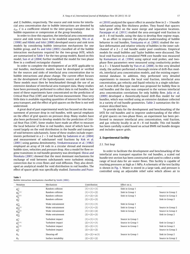
In order to close this equation, the interfacial area concentrationsource and sink terms have to be modeled separately. Wu et al.(1998) and Hibiki and Ishii (2000) developed source and sink termmodels by considering bubble interaction mechanisms for onebubble group, and Fu and Ishii (2003) classified all of the bubbleinteraction mechanisms required for the two-group IATE, whichare summarized in Table 1 for the two-group models. Based on thismodel, Sun et al (2004) further modified the model for two phaseflow in a confined rectangular channel.

In order to complete the development of an IATE applicable torod bundles, mechanistic models must be developed or verifiedfor the sources and sinks of interfacial area concentration due tobubble interactions and phase change. The current effort focuseson the development of the hydrodynamic source and sink terms.These models must then be benchmarked through the use of anextensive database of interfacial area transport data. Many studieshave been previously performed to collect data in rod bundles, butmost of these experiments have concentrated on the prediction ofCritical Heat Flux (CHF) and void fraction measurement. Thus verylittle data is available regarding quantities of interest for interfacialarea transport, and the effect of grid spacers on the flow is not wellunderstood.

A great deal of past experimental work has focused on the mea-surement of pressure drop in rod bundles, with special emphasison the effect of grid spacers on pressure drop. Many studies havealso been performed to develop models for the prediction of Criti-cal Heat Flux (CHF). Some studies have made an effort to measurethe local behavior of flow in rod bundles, most of which have fo-cused largely on the void distribution in the bundle and transportof void between subchannels. Some of these studies include exper-iments performed in a 2 � 3 rod bundle by Sadatomi et al. (2004)and measurement of subchannel void fractions by Kok et al.(2001) using gamma densitometry. Venkateswararao et al. (1982)employed an array of 24 rods in a circular shroud and measuredbubble sizes, velocities and pressure drop. Also a model for flow re-gime transitions in rod bundle geometry was developed. Shirai andNinokata (2001) showed that the most dominant mechanisms forexchange of void between subchannels were turbulent mixing,convection due to cross flows and void diffusion. They also devel-oped an analytical model for void distribution in rod bundles. Theeffect of spacer grids was specifically studied. Damsohn and Prass-

Table 1Bubble interaction mechanisms classified by Smith (2002).

Notation Mechanism Contribution

Rð1ÞRCRandom collision (1) + (1) = (1)

Rð11;2ÞRC

Random collision (1) + (1) = (2)

Rð12;2ÞRC

Random collision (1) + (2) = (2)

Rð2ÞRCRandom collision (2) + (2) = (2)

Rð1ÞWEWake entrainment (1) + (1) = (1)

Rð11;2ÞWE

Wake entrainment (1) + (1) = (2)

Rð12;2ÞWE

Wake entrainment (1) + (2) = (2)

Rð2ÞWEWake entrainment (2) + (2) = (2)

Rð1ÞTITurbulent impact (1) = (1) + (1)

Rð2;11ÞTI

Turbulent impact (2) = (1) + (1)

Rð2;12ÞTI

Turbulent impact (2) = (2) + (1)

Rð2ÞTITurbulent impact (2) = (2) + (2)

RSo Shearing-off (2) = (2) + n�(1

RSI Surface instability (2) = (2) + (2)

er (2010) analyzed the spacer effect in annular flow in 2 � 3 bundlesubchannel using film thickness probes. They found that spacershave great effect on the wave merge and separation locations.Paranjape et al. (2011) studied the area-averaged void fraction inan 8 � 8 rod bundle, using the data to develop flow regime maps.

In an effort to improve the physical understanding of bubblebehavior in rod bundles, Tomiyama et al. (2003) studied the sur-face deformation and relative velocity of bubbles in the inner sub-channel of a 2 � 2 rod bundle under pool conditions. Empiricalmodels for small bubbles and Taylor bubbles were discussed. Thelocal void fraction in a simulated PWR core bundle was measuredby Kumamaru et al. (1994) using optical void probes, and two-phase flow parameters were measured using conductivity probesin a 3 � 3 heated bundle by Yun et al. (2008). In this very detailedstudy, the authors performed a thorough review of drift-flux mod-els, interfacial area concentration models, and the existing experi-mental database. In addition, they performed very detailedexperiments to measure the local void fraction, interfacial areaconcentration, gas velocity and liquid velocity in a single subchan-nel. A new drift-flux type model was proposed for bubbly flow inrod bundles and the data was compared to the various interfacialarea concentration correlations for only bubbly flow. Julia et al.(2009) developed a theoretically-based drift-flux model for rodbundles, which was verified using an extensive database collectedin a variety of rod bundle geometries. Table 2 summarizes the lit-erature described here.

To provide data for the development and benchmarking of theIATE for rod bundles and to improve understanding of the effectof grid spacers on two-phase flows, an experiment has been per-formed to measure interfacial area concentration, void fraction,and gas velocity locally in an 8 � 8 rod bundle. This rod bundlehas been carefully scaled based on actual BWR rod bundle designsand includes spacer grids.

2. Experimental facility

2.1. Test loop

In order to facilitate the development and benchmarking of theinterfacial area transport equation for rod bundles, a scaled rodbundle test section has been constructed and used to collect a widerange of local data for air–water flows. This facility is capable ofreaching pressures as high as 1 MPa. A schematic of the test facilityis shown in Fig. 1. Water is stored in a large tank, and pressure iscontrolled using an adjustable relief valve which allows air to

Effect on ai

Sink in Group 1

Sink in Group 1 Source in Group 2


Sink in Group 2

Sink in Group 1



Sink in Group 2

Source in Group 1

Source in Group 1 Sink in Group 2

Source in Group 1 Sink in Group 2

Source in Group 2

) Source in Group 1 Sink in Group 2

Source in Group 2

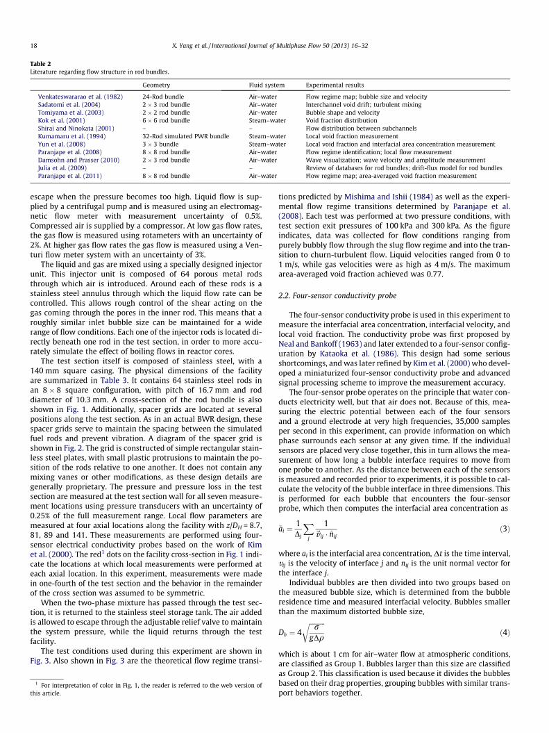
Table 2Literature regarding flow structure in rod bundles.

Geometry Fluid system Experimental results

Venkateswararao et al. (1982) 24-Rod bundle Air–water Flow regime map; bubble size and velocitySadatomi et al. (2004) 2 � 3 rod bundle Air–water Interchannel void drift; turbulent mixingTomiyama et al. (2003) 2 � 2 rod bundle Air–water Bubble shape and velocityKok et al. (2001) 6 � 6 rod bundle Steam–water Void fraction distributionShirai and Ninokata (2001) – – Flow distribution between subchannelsKumamaru et al. (1994) 32-Rod simulated PWR bundle Steam–water Local void fraction measurementYun et al. (2008) 3 � 3 bundle Steam–water Local void fraction and interfacial area concentration measurementParanjape et al. (2008) 8 � 8 rod bundle Air–water Flow regime identification; local flow measurementDamsohn and Prasser (2010) 2 � 3 rod bundle Air–water Wave visualization; wave velocity and amplitude measurementJulia et al. (2009) – – Review of databases for rod bundles; drift-flux model for rod bundlesParanjape et al. (2011) 8 � 8 rod bundle Air–water Flow regime map; area-averaged void fraction measurement

18 X. Yang et al. / International Journal of Multiphase Flow 50 (2013) 16–32

escape when the pressure becomes too high. Liquid flow is sup-plied by a centrifugal pump and is measured using an electromag-netic flow meter with measurement uncertainty of 0.5%.Compressed air is supplied by a compressor. At low gas flow rates,the gas flow is measured using rotameters with an uncertainty of2%. At higher gas flow rates the gas flow is measured using a Ven-turi flow meter system with an uncertainty of 3%.

The liquid and gas are mixed using a specially designed injectorunit. This injector unit is composed of 64 porous metal rodsthrough which air is introduced. Around each of these rods is astainless steel annulus through which the liquid flow rate can becontrolled. This allows rough control of the shear acting on thegas coming through the pores in the inner rod. This means that aroughly similar inlet bubble size can be maintained for a widerange of flow conditions. Each one of the injector rods is located di-rectly beneath one rod in the test section, in order to more accu-rately simulate the effect of boiling flows in reactor cores.

The test section itself is composed of stainless steel, with a140 mm square casing. The physical dimensions of the facilityare summarized in Table 3. It contains 64 stainless steel rods inan 8 � 8 square configuration, with pitch of 16.7 mm and roddiameter of 10.3 mm. A cross-section of the rod bundle is alsoshown in Fig. 1. Additionally, spacer grids are located at severalpositions along the test section. As in an actual BWR design, thesespacer grids serve to maintain the spacing between the simulatedfuel rods and prevent vibration. A diagram of the spacer grid isshown in Fig. 2. The grid is constructed of simple rectangular stain-less steel plates, with small plastic protrusions to maintain the po-sition of the rods relative to one another. It does not contain anymixing vanes or other modifications, as these design details aregenerally proprietary. The pressure and pressure loss in the testsection are measured at the test section wall for all seven measure-ment locations using pressure transducers with an uncertainty of0.25% of the full measurement range. Local flow parameters aremeasured at four axial locations along the facility with z/DH = 8.7,81, 89 and 141. These measurements are performed using four-sensor electrical conductivity probes based on the work of Kimet al. (2000). The red1 dots on the facility cross-section in Fig. 1 indi-cate the locations at which local measurements were performed ateach axial location. In this experiment, measurements were madein one-fourth of the test section and the behavior in the remainderof the cross section was assumed to be symmetric.

When the two-phase mixture has passed through the test sec-tion, it is returned to the stainless steel storage tank. The air addedis allowed to escape through the adjustable relief valve to maintainthe system pressure, while the liquid returns through the testfacility.

The test conditions used during this experiment are shown inFig. 3. Also shown in Fig. 3 are the theoretical flow regime transi-

1 For interpretation of color in Fig. 1, the reader is referred to the web version ofthis article.

tions predicted by Mishima and Ishii (1984) as well as the experi-mental flow regime transitions determined by Paranjape et al.(2008). Each test was performed at two pressure conditions, withtest section exit pressures of 100 kPa and 300 kPa. As the figureindicates, data was collected for flow conditions ranging frompurely bubbly flow through the slug flow regime and into the tran-sition to churn-turbulent flow. Liquid velocities ranged from 0 to1 m/s, while gas velocities were as high as 4 m/s. The maximumarea-averaged void fraction achieved was 0.77.

2.2. Four-sensor conductivity probe

The four-sensor conductivity probe is used in this experiment tomeasure the interfacial area concentration, interfacial velocity, andlocal void fraction. The conductivity probe was first proposed byNeal and Bankoff (1963) and later extended to a four-sensor config-uration by Kataoka et al. (1986). This design had some seriousshortcomings, and was later refined by Kim et al. (2000) who devel-oped a miniaturized four-sensor conductivity probe and advancedsignal processing scheme to improve the measurement accuracy.

The four-sensor probe operates on the principle that water con-ducts electricity well, but that air does not. Because of this, mea-suring the electric potential between each of the four sensorsand a ground electrode at very high frequencies, 35,000 samplesper second in this experiment, can provide information on whichphase surrounds each sensor at any given time. If the individualsensors are placed very close together, this in turn allows the mea-surement of how long a bubble interface requires to move fromone probe to another. As the distance between each of the sensorsis measured and recorded prior to experiments, it is possible to cal-culate the velocity of the bubble interface in three dimensions. Thisis performed for each bubble that encounters the four-sensorprobe, which then computes the interfacial area concentration as

�ai ¼1Dj

Xj

1~v ij � n̂ij

ð3Þ

where ai is the interfacial area concentration, Dt is the time interval,vij is the velocity of interface j and nij is the unit normal vector forthe interface j.

Individual bubbles are then divided into two groups based onthe measured bubble size, which is determined from the bubbleresidence time and measured interfacial velocity. Bubbles smallerthan the maximum distorted bubble size,

Db ¼ 4ffiffiffiffiffiffiffiffiffiffir

gDq

rð4Þ

which is about 1 cm for air–water flow at atmospheric conditions,are classified as Group 1. Bubbles larger than this size are classifiedas Group 2. This classification is used because it divides the bubblesbased on their drag properties, grouping bubbles with similar trans-port behaviors together.

Fig. 1. Schematic of test facility.


All measurement methods carry some degree of uncertainty.For the four-sensor conductivity probe, an extensive uncertaintyanalysis was performed by Kim et al. (2000). Essentially, this typeof probe has two major sources of uncertainty when measuringvelocity. The first source of uncertainty is due to the geometry ofthe probe and is a function of the interface velocity, distance be-tween sensors, and measurement acquisition rate. For the currentexperiment, this error source is 10%. The second source of uncer-tainty is based on the distortion in the bubble interface when itmakes contact with the intrusive probe. From the work of Kimet al. (2000), the uncertainty due to this effect is approximately6%. Thus the total uncertainty of the velocity measurements, and

therefore interfacial area concentration, is 11.6%. The area of thefour-sensor probe is about 0.2 mm2, with a diameter of about0.5 mm, while the total flow area is about 128 cm2. Because theprobe is so small compared to the total flow area, no significantflow disturbance is expected downstream of the probe. When mea-suring void fraction, the uncertainty is dependent on the bubblefrequency and measurement time and is approximately 5%.

These experimental uncertainties can be evaluated by compar-ing the gas flux measured using local conductivity probes to thatmeasured by the Venturi mass flow meter. This type of analysisis only valid for flows in which most of the gas is represented bysmall spherical bubbles. As the surface of large Group 2 bubbles

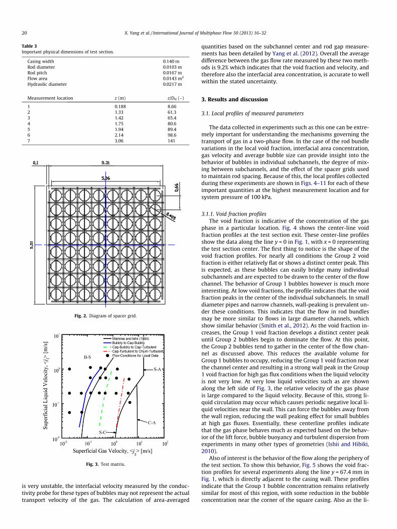
Table 3Important physical dimensions of test section.

Casing width 0.140 mRod diameter 0.0103 mRod pitch 0.0167 mFlow area 0.0143 m2

Hydraulic diameter 0.0217 m

Measurement location z (m) z/DH (–)

1 0.188 8.662 1.33 61.33 1.42 65.44 1.75 80.65 1.94 89.46 2.14 98.67 3.06 141

Fig. 2. Diagram of spacer grid.

Fig. 3. Test matrix.


is very unstable, the interfacial velocity measured by the conduc-tivity probe for these types of bubbles may not represent the actualtransport velocity of the gas. The calculation of area-averaged

quantities based on the subchannel center and rod gap measure-ments has been detailed by Yang et al. (2012). Overall the averagedifference between the gas flow rate measured by these two meth-ods is 9.2% which indicates that the void fraction and velocity, andtherefore also the interfacial area concentration, is accurate to wellwithin the stated uncertainty.

3. Results and discussion

3.1. Local profiles of measured parameters

The data collected in experiments such as this one can be extre-mely important for understanding the mechanisms governing thetransport of gas in a two-phase flow. In the case of the rod bundlevariations in the local void fraction, interfacial area concentration,gas velocity and average bubble size can provide insight into thebehavior of bubbles in individual subchannels, the degree of mix-ing between subchannels, and the effect of the spacer grids usedto maintain rod spacing. Because of this, the local profiles collectedduring these experiments are shown in Figs. 4–11 for each of theseimportant quantities at the highest measurement location and forsystem pressure of 100 kPa.

3.1.1. Void fraction profilesThe void fraction is indicative of the concentration of the gas

phase in a particular location. Fig. 4 shows the center-line voidfraction profiles at the test section exit. These center-line profilesshow the data along the line y = 0 in Fig. 1, with x = 0 representingthe test section center. The first thing to notice is the shape of thevoid fraction profiles. For nearly all conditions the Group 2 voidfraction is either relatively flat or shows a distinct center peak. Thisis expected, as these bubbles can easily bridge many individualsubchannels and are expected to be drawn to the center of the flowchannel. The behavior of Group 1 bubbles however is much moreinteresting. At low void fractions, the profile indicates that the voidfraction peaks in the center of the individual subchannels. In smalldiameter pipes and narrow channels, wall-peaking is prevalent un-der these conditions. This indicates that the flow in rod bundlesmay be more similar to flows in large diameter channels, whichshow similar behavior (Smith et al., 2012). As the void fraction in-creases, the Group 1 void fraction develops a distinct center peakuntil Group 2 bubbles begin to dominate the flow. At this point,the Group 2 bubbles tend to gather in the center of the flow chan-nel as discussed above. This reduces the available volume forGroup 1 bubbles to occupy, reducing the Group 1 void fraction nearthe channel center and resulting in a strong wall peak in the Group1 void fraction for high gas flux conditions when the liquid velocityis not very low. At very low liquid velocities such as are shownalong the left side of Fig. 3, the relative velocity of the gas phaseis large compared to the liquid velocity. Because of this, strong li-quid circulation may occur which causes periodic negative local li-quid velocities near the wall. This can force the bubbles away fromthe wall region, reducing the wall peaking effect for small bubblesat high gas fluxes. Essentially, these centerline profiles indicatethat the gas phase behaves much as expected based on the behav-ior of the lift force, bubble buoyancy and turbulent dispersion fromexperiments in many other types of geometries (Ishii and Hibiki,2010).

Also of interest is the behavior of the flow along the periphery ofthe test section. To show this behavior, Fig. 5 shows the void frac-tion profiles for several experiments along the line y = 67.4 mm inFig. 1, which is directly adjacent to the casing wall. These profilesindicate that the Group 1 bubble concentration remains relativelysimilar for most of this region, with some reduction in the bubbleconcentration near the corner of the square casing. Also as the li-

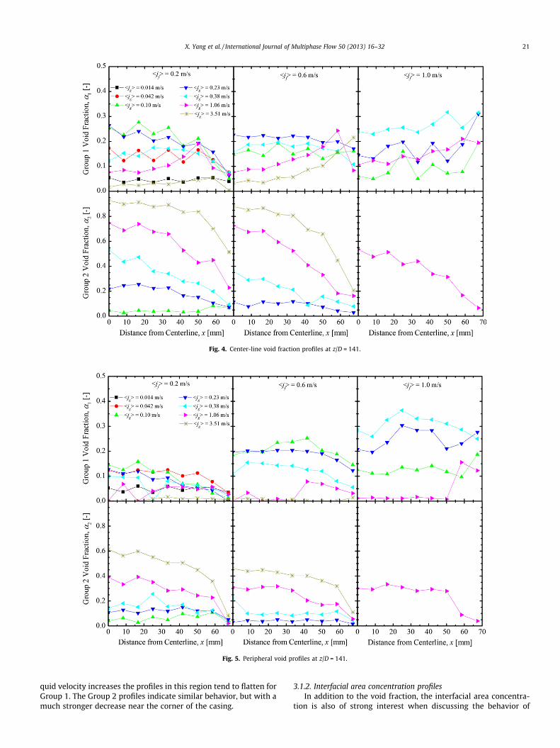
Fig. 4. Center-line void fraction profiles at z/D = 141.

Fig. 5. Peripheral void profiles at z/D = 141.


quid velocity increases the profiles in this region tend to flatten forGroup 1. The Group 2 profiles indicate similar behavior, but with amuch stronger decrease near the corner of the casing.

3.1.2. Interfacial area concentration profilesIn addition to the void fraction, the interfacial area concentra-

tion is also of strong interest when discussing the behavior of

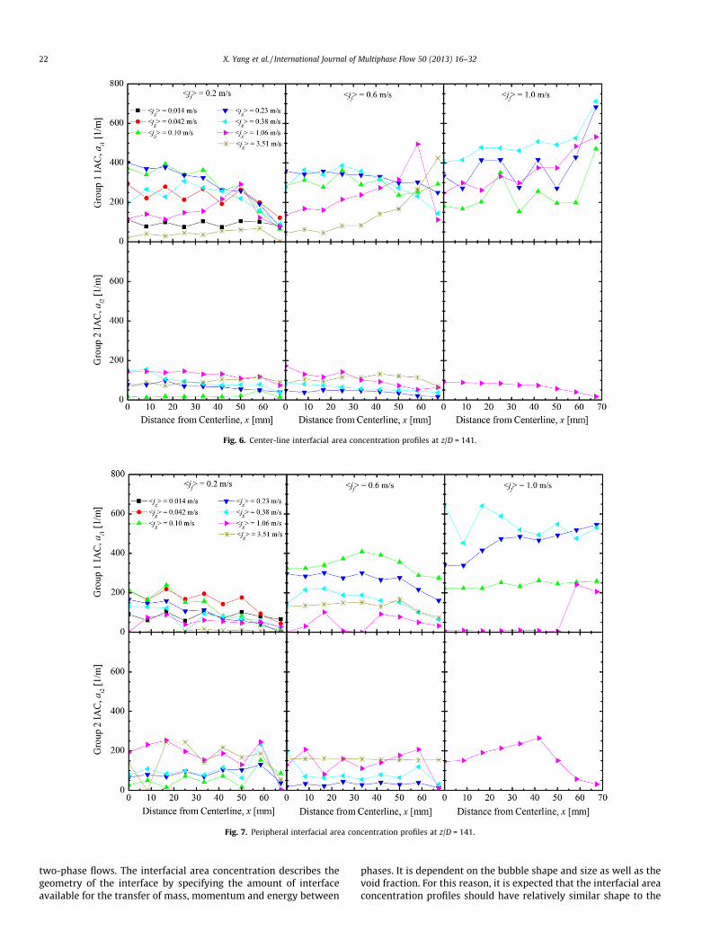
Fig. 6. Center-line interfacial area concentration profiles at z/D = 141.

Fig. 7. Peripheral interfacial area concentration profiles at z/D = 141.


two-phase flows. The interfacial area concentration describes thegeometry of the interface by specifying the amount of interfaceavailable for the transfer of mass, momentum and energy between

phases. It is dependent on the bubble shape and size as well as thevoid fraction. For this reason, it is expected that the interfacial areaconcentration profiles should have relatively similar shape to the

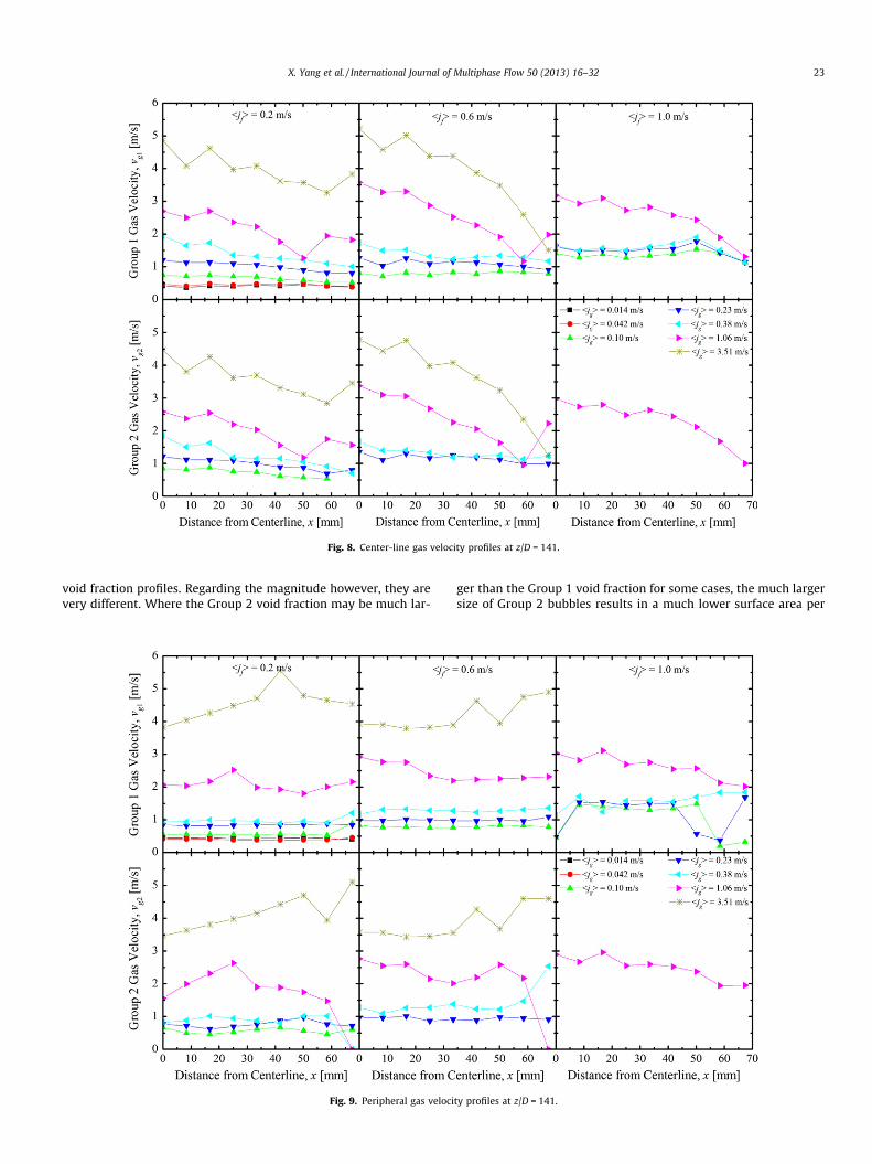
Fig. 8. Center-line gas velocity profiles at z/D = 141.


void fraction profiles. Regarding the magnitude however, they arevery different. Where the Group 2 void fraction may be much lar-

Fig. 9. Peripheral gas veloci

ger than the Group 1 void fraction for some cases, the much largersize of Group 2 bubbles results in a much lower surface area per

ty profiles at z/D = 141.

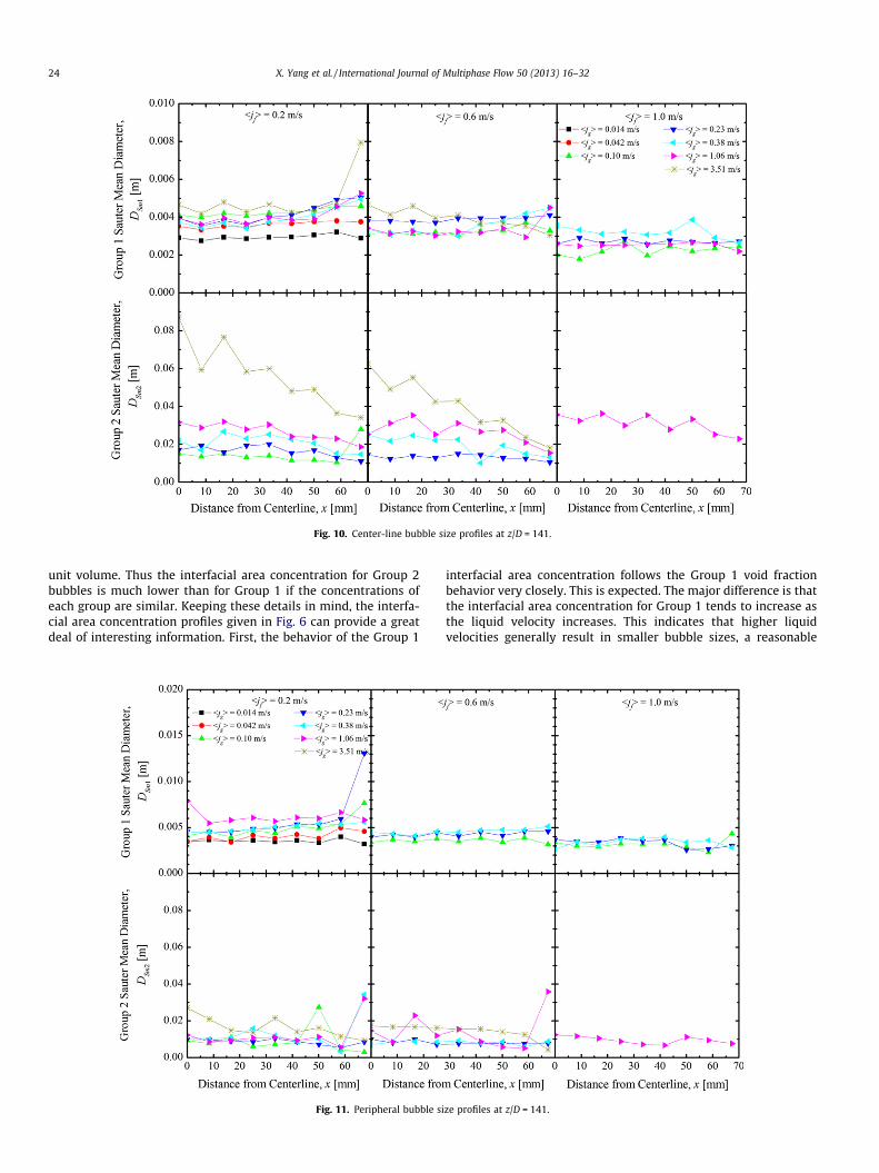
Fig. 10. Center-line bubble size profiles at z/D = 141.


unit volume. Thus the interfacial area concentration for Group 2bubbles is much lower than for Group 1 if the concentrations ofeach group are similar. Keeping these details in mind, the interfa-cial area concentration profiles given in Fig. 6 can provide a greatdeal of interesting information. First, the behavior of the Group 1

Fig. 11. Peripheral bubble si

interfacial area concentration follows the Group 1 void fractionbehavior very closely. This is expected. The major difference is thatthe interfacial area concentration for Group 1 tends to increase asthe liquid velocity increases. This indicates that higher liquidvelocities generally result in smaller bubble sizes, a reasonable

ze profiles at z/D = 141.


conclusion as higher liquid velocities generally cause more intenseturbulence. For Group 2 however, the interfacial area concentra-tion is relatively constant across the entire flow area. As Fig. 4shows that the void fraction decreases as one approaches the chan-nel wall, this flat profile indicates that the Group 2 bubble size islargest in the center of the flow channel and decreases near thechannel wall. Also, the size of the Group 2 interfacial area concen-tration tends to reach a maximum at gas velocity of about 1.0 m/s.For higher gas flux conditions coalescence of Group 2 bubbles in-creases, leading to larger bubbles in the transition to churn-turbu-lent in annular flow and decreasing the interfacial areaconcentration.

The profiles near the flow channel wall are also of interest forinterfacial area concentration and are shown in Fig. 7. Once again,the Group 1 profile for interfacial area concentration closely fol-lows the Group 1 void fraction profile. This indicates that the bub-ble size is relatively constant. For lower gas flux conditions, theGroup 2 interfacial area concentration is similar near the peripheryand in the channel center. As the gas flux increases however, theGroup 2 bubbles near the channel center become much larger,resulting in a smaller interfacial area concentration in this regionand resulting in smaller Group 2 bubbles occupying the region nearthe wall. This results in higher interfacial area concentration forGroup 2 on the channel periphery than in the channel center ex-cept very near the corner of the square casing. Once again, the dataagrees well with the trends expected based on the various forcesacting on the bubbles (Ishii and Hibiki, 2010).

3.1.3. Gas velocity profilesThe third major parameter of interest when analyzing the local

behavior of two-phase flows is the interfacial velocity. The four-sensor probes used in this study measure the interfacial velocityfor the purpose of determining the interfacial area concentration.For Group 1 bubbles, this interfacial velocity is approximately thesame as the bulk gas velocity. This is because such small bubbleshave relatively rigid, spherical surfaces. For this reason, the Group1 interfacial velocity is expected to very closely correlate to the li-quid velocity profile. Group 2 bubbles, on the other hand, have rel-atively unstable surfaces and can change shape very readily. Thusthe interfacial velocity measured by the four-sensor probe maynot be the same as the gas transport velocity for very large bubbles.This must be kept in mind when analyzing the results of the veloc-ity measurements. Fig. 8 shows the center-line profile of the gasvelocity measurement. As expected, the Group 1 gas velocity pro-vides a reasonable estimate for the liquid flow rate. At low voidfraction, the velocity profiles for both bubble groups are much flat-ter than those noted for smaller-diameter pipes. This is likely dueto the effect of the rod bundle, which provides a great deal of inter-nal surface area. This internal surface area increases the friction be-tween the liquid and structure and tends to flatten the liquidvelocity profile. At higher void fractions however, the velocity pro-file develops a strong center peak. This is due to the action of Group2 bubbles, which have a large relative velocity compared to Group1 bubbles and tend to gather in the center of the flow channel. As aresult, the mixture flows more quickly in this region and moreslowly near the channel wall.

The gas velocity measurements near the channel periphery,shown in Fig. 9 also provide some interesting information. In thisexperiment the velocity profiles for both bubble groups near thewall are relatively flat as expected, but they also show much highervelocity than would be expected near the flow channel wall for sin-gle-phase flow with a turbulent velocity profile. As described abovethis is due to the flow channel geometry, which results in a flattervelocity profile than in pipe flow. Further, because of the no-slipcondition and the presence of rods the liquid velocity gradient nearthe wall is very large. This results in the flow reaching relatively

high velocities, even near the flow channel wall. Additionally, thismay result in increased production of turbulent kinetic energy.This may result in smaller bubble sizes and even flatter velocityprofiles and can enhance bubble transport and mixing betweensubchannels.

3.1.4. Bubble Sauter mean diameter profilesThe final major parameter of interest in two-phase flows is the

bubble size. In this experiment, the bubble size is measured by theSauter mean diameter, which is closely related to the void fractionand interfacial area concentration and represents the spherical-equivalent diameter. This means that the Sauter mean diameteris the diameter of a sphere with the same volume-to-surface-arearatio as the average for each bubble group. The center-line profilesof Sauter mean diameter are shown in Fig. 10. For Group 1 bubbles,the Sauter mean diameter is relatively constant across the flowchannel. Generally, it is expected that the bubble size should de-crease significantly in the region of the flow channel wall. The rea-son this trend is not shown here is that due to the presence of therods, nearly the entire flow area is near the flow channel wall. Thisresults in little change in bubble size across the flow channel forthese small bubbles. Additionally, the bubble size tends to increaseas the gas flow rate increases due to enhanced bubble coalescence.At the same time, the bubble size tends to decrease as the liquidvelocity increases due to enhanced bubble breakup due to turbu-lence. Group 2 bubbles show a slight decrease in size near the flowchannel wall. As these bubbles are capable of bridging several sub-channels, they are less restricted by the existence of so many sur-faces and tend to concentrate near the center of the flow channel. Itshould also be noted that the size of these bubbles is relativelyindependent of the liquid velocity. Group 2 bubbles are generallymuch larger than the characteristic turbulent eddies. Because ofthis, they are less strongly affected by the changes in turbulenceas the liquid velocity changes. This means much smaller changesin the coalescence and breakup frequencies and therefore muchless effect on the bubble size than for Group 1 bubbles. Further,the Group 2 bubble size continues to increase as the void fractionincreases. This is expected and indicates that bubble coalescenceincreases due to the higher concentration of Group 2 bubbles.

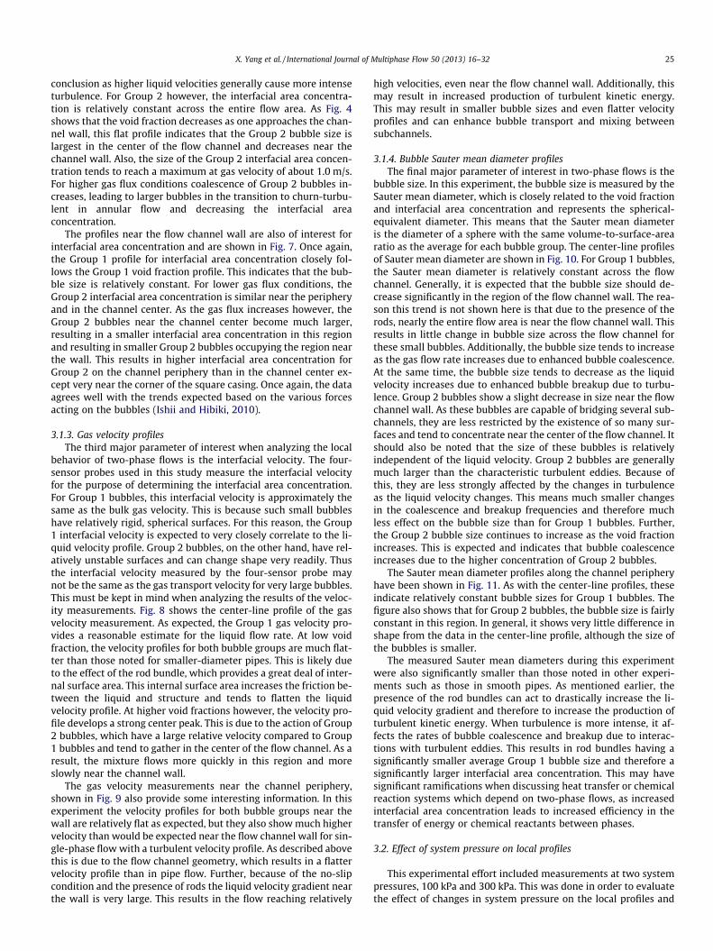
The Sauter mean diameter profiles along the channel peripheryhave been shown in Fig. 11. As with the center-line profiles, theseindicate relatively constant bubble sizes for Group 1 bubbles. Thefigure also shows that for Group 2 bubbles, the bubble size is fairlyconstant in this region. In general, it shows very little difference inshape from the data in the center-line profile, although the size ofthe bubbles is smaller.

The measured Sauter mean diameters during this experimentwere also significantly smaller than those noted in other experi-ments such as those in smooth pipes. As mentioned earlier, thepresence of the rod bundles can act to drastically increase the li-quid velocity gradient and therefore to increase the production ofturbulent kinetic energy. When turbulence is more intense, it af-fects the rates of bubble coalescence and breakup due to interac-tions with turbulent eddies. This results in rod bundles having asignificantly smaller average Group 1 bubble size and therefore asignificantly larger interfacial area concentration. This may havesignificant ramifications when discussing heat transfer or chemicalreaction systems which depend on two-phase flows, as increasedinterfacial area concentration leads to increased efficiency in thetransfer of energy or chemical reactants between phases.

3.2. Effect of system pressure on local profiles

This experimental effort included measurements at two systempressures, 100 kPa and 300 kPa. This was done in order to evaluatethe effect of changes in system pressure on the local profiles and


interfacial area concentration. Generally, the most important effectof system pressure is on the expansion of bubbles along the test sec-tion. Bubble expansion is determined by the change in the densityof the gas phase. The relative change in the density of the gas phaseis related to the system pressure and the pressure drop through theideal gas law (as a first approximation), which means that thechange is gas volume is a function of the ratio of pressure drop tosystem pressure. For a given flow velocity, the pressure drop willbe very similar regardless of system pressure. Thus when the sys-tem pressure is increased from 100 kPa to 300 kPa the expansionof the gas is drastically reduced. This has a wide variety of effects.

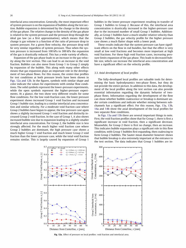
Expansion of the gas phase leads to an increase in the gas veloc-ity along the test section. This can lead to an increase in the voidfraction. Bubbles can also move from Group 1 to Group 2 simplyby expansion of the bubble. This along with many other effectsmeans that gas expansion plays an important role in the develop-ment of two-phase flows. For this reason, the center-line profilesfor test conditions at both pressure levels have been shown inFigs. 12a and 12b. In the figures, symbols with similar shape andcolor indicate the values for experiments with similar flow condi-tions. The solid symbols represent the lower-pressure experiments,while the open symbols represent the higher-pressure experi-ments. At a glance, the two show very different results for someflow conditions. For the low void-fraction case, the lower pressureexperiment shows increased Group 1 void fraction and increasedGroup 1 bubble size, leading to a similar interfacial area concentra-tion and similar velocity. For a moderate void fraction case whereGroup 2 bubbles have begun to appear, the low pressure case againshows a slightly increased Group 1 void fraction and distinctly in-creased Group 2 void fraction. In the case of Group 1, it also showsincreased bubble size due to expansion leading to a slightly smallerinterfacial area concentration. For Group 2, the bubble size is lessstrongly affected. For the much higher void fraction case whereGroup 2 bubbles are dominant, the high pressure case shows amuch higher Group 1 void fraction and much lower Group 2 voidfraction than the lower pressure case, while the total void fractionremains similar. This is largely caused by expansion of Group 1

Fig. 12a. Effect of pressure on local profil

bubbles in the lower-pressure experiment resulting in transfer ofGroup 1 bubbles to Group 2. Because of this, the interfacial areaconcentration is drastically increased in the higher-pressure casedue to the increased number of small Group 1 bubbles. Addition-ally, as Group 1 bubbles have a much smaller relative velocity thanGroup 2 bubbles, the gas velocity profile for the higher pressurecase shows a much flatter shape with a lower peak.

These results indicate that the system pressure can have signif-icant effects on the flow in rod bundles, but that the effect is verysmall at low void fractions and becomes more important at highvoid fractions. For these high void fraction cases, increasing pres-sure limits expansion of the gas phase. This leads to decreased bub-ble size, which can increase the interfacial area concentration andhave a significant effect on the velocity profile.

3.3. Axial development of local profiles

The fully-developed local profiles are valuable tools for deter-mining the basic hydrodynamics two-phase flows, but they donot provide the entire picture. In addition to this data, the develop-ment of the local profiles along the test section can also provideessential information regarding the dynamic behavior of two-phase flows. Information regarding the development of the flowcan show whether bubble coalescence or breakup is dominant un-der certain conditions and indicate whether mixing between sub-channels has a significant effect. For this reason, Figs. 13a, 13b,14a and 14b show the axial development of the local profiles fortwo separate flow conditions.

In Figs. 13a and 13b there are several important things to note.First, the void fraction profiles show that for Group 1, there is first asignificant increase in void fraction, then a significant decrease.Meanwhile, for Group 2 there is first no change, then an increase.This indicates bubble expansion plays a significant role in this flowcondition, with Group 1 bubbles first expanding, then coalescing toform Group 2 bubbles. The Sauter mean diameter however showsthat bubble breakup is also extremely important at the entrance tothe test section. The data indicates that Group 1 bubbles are in-

es: void fraction and interfacial area.

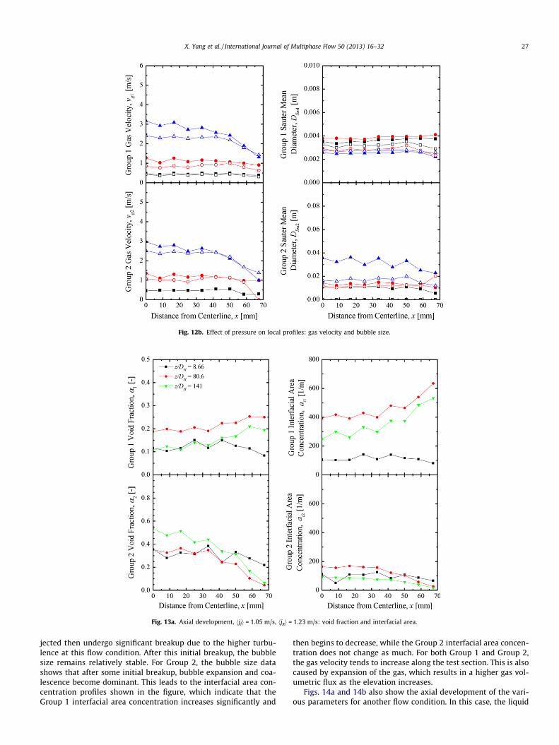
Fig. 12b. Effect of pressure on local profiles: gas velocity and bubble size.

Fig. 13a. Axial development, hjfi = 1.05 m/s, hjgi = 1.23 m/s: void fraction and interfacial area.


jected then undergo significant breakup due to the higher turbu-lence at this flow condition. After this initial breakup, the bubblesize remains relatively stable. For Group 2, the bubble size datashows that after some initial breakup, bubble expansion and coa-lescence become dominant. This leads to the interfacial area con-centration profiles shown in the figure, which indicate that theGroup 1 interfacial area concentration increases significantly and

then begins to decrease, while the Group 2 interfacial area concen-tration does not change as much. For both Group 1 and Group 2,the gas velocity tends to increase along the test section. This is alsocaused by expansion of the gas, which results in a higher gas vol-umetric flux as the elevation increases.

Figs. 14a and 14b also show the axial development of the vari-ous parameters for another flow condition. In this case, the liquid

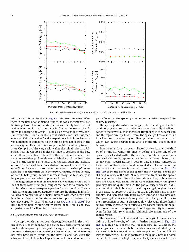
Fig. 13b. Axial development, hjfi = 1.05 m/s, hjgi = 1.23 m/s: gas velocity and bubble size.


velocity is much smaller than in Fig. 13. This results in many differ-ences in the flow development during these two experiments. First,the Group 1 void fraction tends to decrease sharply from the testsection inlet, while the Group 2 void fraction increases signifi-cantly. In addition, the Group 1 bubble size remains relatively con-stant while the Group 2 bubble size is initially constant, but thenincreases. This shows that for this experiment bubble coalescencewas dominant as compared to the bubble breakup shown in theprevious figure. This results in Group 1 bubbles combining to formlarger Group 2 bubbles very rapidly after the initial injection. Fol-lowing this, the Group 2 bubbles continue to coalesce as the flowpasses through the test section. This then results in the interfacialarea concentration profiles shown, which show a large initial de-crease in the Group 1 interfacial area concentration and increasein Group 2 interfacial area concentration, followed by little changein the Group 1 value and a continued decrease in the Group 2 inter-facial area concentration. As in the previous figure, the gas velocityfor both bubble groups tends to increase along the test facility asthe gas phase expands due to pressure losses.

The large differences in the dynamic development of the flow ineach of these cases strongly highlights the need for a comprehen-sive interfacial area transport equation for rod bundles. Currentstatic correlations cannot accurately capture the change in interfa-cial area concentration as bubbles interact with each other aftertheir initial formation. Interfacial area transport equations havebeen developed for small-diameter pipes (Fu and Ishii, 2003) butthese models predict significantly larger bubble sizes and maynot perform well for flows in rod bundles.

3.4. Effect of spacer grid on local flow parameters

One topic which has not been thoroughly treated in the litera-ture is the effect of the spacer grid on the two-phase flows. At theirsimplest these spacer grids are just blockages to the flow, but manycommercial designs include mixing vanes or other special featuresthat may have large effects on the flow. In addition, even thebehavior of simple flow blockages is not well understood in two-

phase flows and the spacer grid represents a rather complex formof flow blockage.

The spacer grids can have varying effects depending on the flowcondition, system pressure, and other factors. Generally the distur-bance to the flow results in increased turbulence in the spacer gridand the region directly downstream. The spacer grid can also resultin a low-pressure wake region directly behind the metal vaneswhich can cause recirculation and significantly affect bubblebehavior.

Experimental data has been collected at two locations, with z/DH of 81 and 89, which are directly before and after one of thespacer grids located within the test section. These spacer gridsare relatively simple, representative designs without mixing vanesor any other special features. Despite this, the data collected atthese two locations can provide a great deal of information onthe behavior of the flow in the region near the spacer. Figs. 15aand 15b show the effect of the spacer grid for several conditionsat liquid velocity of 0.2 m/s. At very low void fractions, the spacerhas very limited effect. Since the flow rate is so low, turbulence ef-fects are already very small and the wake region behind the spacergrid may also be quite small. As the gas velocity increases, a dis-tinct trend of bubble breakup over the spacer grid region is seen.In this case, the spacer grid cuts large Group 2 bubbles into smallerbubbles, and increased turbulence causes some additional breakup.The spacer grid also acts to homogenize the velocity profile due tothe introduction of such a dispersed flow blockage. These factorsact to slightly increase the interfacial area concentration in the re-gion downstream of the spacer grid. As the gas velocity is increaseseven further this trend remains although the magnitude of thechange varies.

The behavior of the flow around the spacer grid for several con-ditions at liquid velocity of 1 m/s is further illustrated in Figs. 16aand 16b. This figure shows that for moderate gas velocities, thespacer grid causes overall bubble coalescence as indicated by theincreased bubble size and decreased Group 1 void fraction follow-ing the spacer grid. This is in contrast to the bubble breakup notedearlier. In this case, the higher liquid velocity causes a much stron-

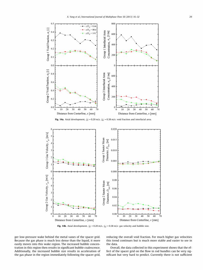
Fig. 14a. Axial development, hjfi = 0.20 m/s, hjgi = 0.38 m/s: void fraction and interfacial area.

Fig. 14b. Axial development, hjfi = 0.20 m/s, hjgi = 0.38 m/s: gas velocity and bubble size.


ger low-pressure wake behind the metal vanes of the spacer grid.Because the gas phase is much less dense than the liquid, it moreeasily moves into this wake region. The increased bubble concen-tration in this region then results in significant bubble coalescence.Additionally, the increased bubble size results in acceleration ofthe gas phase in the region immediately following the spacer grid,

reducing the overall void fraction. For much higher gas velocitiesthis trend continues but is much more stable and easier to see inthe data.

Overall, the data collected in this experiment shows that the ef-fect of the spacer grid on the flow in rod bundles can be very sig-nificant but very hard to predict. Currently there is not sufficient

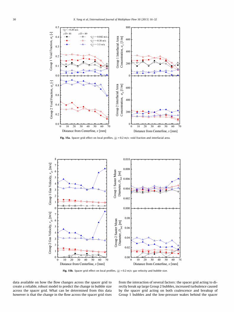
Fig. 15a. Spacer grid effect on local profiles, hjfi = 0.2 m/s: void fraction and interfacial area.

Fig. 15b. Spacer grid effect on local profiles, hjfi = 0.2 m/s: gas velocity and bubble size.


data available on how the flow changes across the spacer grid tocreate a reliable, robust model to predict the change in bubble sizeacross the spacer grid. What can be determined from this datahowever is that the change in the flow across the spacer grid rises

from the interaction of several factors: the spacer grid acting to di-rectly break up large Group 2 bubbles, increased turbulence causedby the spacer grid acting on both coalescence and breakup ofGroup 1 bubbles and the low-pressure wakes behind the spacer

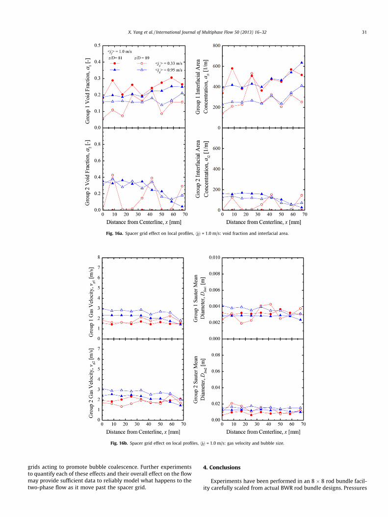
Fig. 16a. Spacer grid effect on local profiles, hjfi = 1.0 m/s: void fraction and interfacial area.

Fig. 16b. Spacer grid effect on local profiles, hjfi = 1.0 m/s: gas velocity and bubble size.


grids acting to promote bubble coalescence. Further experimentsto quantify each of these effects and their overall effect on the flowmay provide sufficient data to reliably model what happens to thetwo-phase flow as it move past the spacer grid.

4. Conclusions

Experiments have been performed in an 8 � 8 rod bundle facil-ity carefully scaled from actual BWR rod bundle designs. Pressures


of 100 kPa and 300 kPa were used, and local profiles of void frac-tion, interfacial area concentration and gas velocity were measuredat four axial conditions for a wide array of flow conditions.

� Valuable experimental data has been provided for the develop-ment and testing of the interfacial area transport equation forrod bundle geometries.� This data has shown that the overall behavior of the flow is sim-

ilar to the behavior of other two-phase flows and that most ofthe differences can be accounted for based on the interactionof the flow with the channel structure, with some exceptions.� The rod bundle geometry may result in larger turbulent inten-

sity than flows in more open geometries, leading to increasedbubble breakup and smaller bubble sizes. This in turn resultsin higher interfacial area concentrations in rod bundles asopposed to circular pipes.� There is a distinct difference in the behavior of the bubble

groups, as the motion of Group 1 bubbles is limited by the indi-vidual subchannels but Group 2 bubbles are largely limited onlyby the casing size. These two length scales must be accountedfor when modeling flows in rod bundles.� The spacer grids used to maintain rod spacing in fuel bundles

can have many effects on two-phase flows including changesto the turbulent behavior of the flow and the creation of low-pressure wake regions. Additional experimentation is requiredin order to fully understand the overall effect these phenomenahave on two-phase flows across spacer grids and in order todevelop accurate models for predicting flows in along rodbundles.

Acknowledgements

This work was performed at Purdue University under the aus-pices of the US Nuclear Regulatory Commission (NRC), Office ofNuclear Regulatory Research, through the Institute of Thermal-Hydraulics.

References

Damsohn, M., Prasser, H.M., 2010. Experimental studies of the effect of functionalspacers to annular flow in subchannels of a BWR fuel element. Nucl. Eng. Des.240, 3126–3144.

Fu, X.Y., Ishii, M., 2003. Two-group interfacial area transport in vertical air–waterflow. I: Mechanistic model. Nucl. Eng. Des. 219, 142–168.

Hibiki, T., Ishii, M., 2000. One-group interfacial area transport of bubbly flows invertical round tubes. Int. J. Heat Mass Transfer 43, 2711–2726.

Ishii, M., Hibiki, T., 2010. Thermo-Fluid Dynamics of Two-Phase Flow. Springer, NY.Julia, J.E., Hibiki, T., Ishii, M., Yun, B.J., Park, G.C., 2009. Drift-flux model in a sub-

channel of rod bundle geometry. Int. J. Heat Mass Transfer 52, 3032–3041.Kataoka, I., Ishii, M., Serizawa, A., 1986. Local formulation and measurement of

interfacial area concentration in two-phase flow. Int. J. Multiphase Flow 12,505–529.

Kim, S., Fu, X.Y., Wang, X., Ishii, M., 2000. Development of the miniaturized four-sensor conductivity probe and the signal processing scheme. Int. J. Heat MassTransfer 43, 4101–4118.

Kocamustafaogullar, G., Ishii, M., 1995. Foundation of the interfacial area transportequation and its closure relations. Int. J. Heat Mass Transfer 38, 481–493.

Kok, H.V., Van Der Hagen, T.H.J.J., Mudde, R.F., 2001. Subchannel void-fractionmeasurements in a 6 by 6 rod bundle using a simple gamma-transmissionmethod. Int. J. Multiphase Flow 27, 147–170.

Kumamaru, H., Kondo, M., Murata, H., Kukita, Y., 1994. Void-fraction distributionunder high-pressure boil-off conditions in rod bundle geometry. Nucl. Eng. Des.150, 95–105.

Mishima, K., Ishii, M., 1984. Flow regime transition criteria for upward two-phaseflow in vertical tubes. Int. J. Heat Mass Transfer 27, 723–737.

Neal, L.G., Bankoff, S.G., 1963. A high resolution resistivity probe for determinationof local void properties in gas–liquid flow. AIChE J. 9, 490–494.

Paranjape, S., Chen, S.W., Hibiki, T., Ishii, M., 2011. Flow regime identification underadiabatic upward two-phase flow in a vertical rod bundle geometry. J. FluidsEng. 133.

Paranjape, S., Stefanczyk, D., Liang, Y., 2008. Global flow regime identification in arod bundle geometry. In: 16th International Conference on Nuclear Engineering,ICONE-16. Orlando, FL, USA. May 11–15, 2008.

Sadatomi, M., Kawahara, A., Kano, K., Tanoue, S., 2004. Flow characteristics inhydraulically equilibrium two-phase flows in a vertical 2 � 3 rod bundle. Int. J.Multiphase Flow 30, 1093–1119.

Shirai, H., Ninokata, H., 2001. Prediction of the equilibrium two-phase flowdistributions in inter-connected subchannel systems. J. Nucl. Sci. Technol. 38,379–387.

Smith, T.R., 2002. Two-Group Interfacial Area Transport Equation in Large DiameterPipes. Ph.D. Thesis, Purdue University, 2002.

Smith, T.R., Schlegel, J.P., Hibiki, T., Ishii, M., 2012. Two-phase flow structure in largediameter pipes. Int. J. Heat Fluid Flow 33, 156–167.

Sun, X., Kim, S., Ishii, M., Beus, S.G., 2004. Modeling of bubble coalescence anddisintegration in confined upward two-phase flow. Nucl. Eng. Des. 230, 3–26.

Tomiyama, A., Nakahara, Y., Adachi, Y., Hosokawa, S., 2003. Shapes and risingvelocities of single bubbles rising through an inner subchannel. J. Nucl. Sci.Technol. 40, 136–142.

Venkateswararao, P., Semiat, R., Dukler, A.E., 1982. Flow pattern transition for gas–liquid flow in a vertical rod bundle. Int. J. Multiphase Flow 8, 509–524.

Wu, Q., Kim, S., Ishii, M., Beus, S.G., 1998. One-group interfacial area transport invertical bubbly flow. Int. J. Heat Mass Transfer 41, 1109–1112.

Yang, X., Schlegel, J.P., Liu, Y., Paranjape, S., Hibiki, T., Ishii, M., 2012. Measurementand modeling of two-phase flow parameters in scaled 8 � 8 BWR rod bundle.Int. J. Heat Fluid Flow 34, 85–97.

Yun, B.J., Park, G.C., Julia, J.E., Hibiki, T., 2008. Flow structure of subcooled boilingwater flow in a subchannel of 3 � 3 rod bundles. J. Nucl. Sci. Technol. 45, 1–21.

experimental study of interfacial area transport in air–water two phase flow in a scaled 8×8 bwr...

Documents