experimental mathematics meets mathematical...
TRANSCRIPT
1
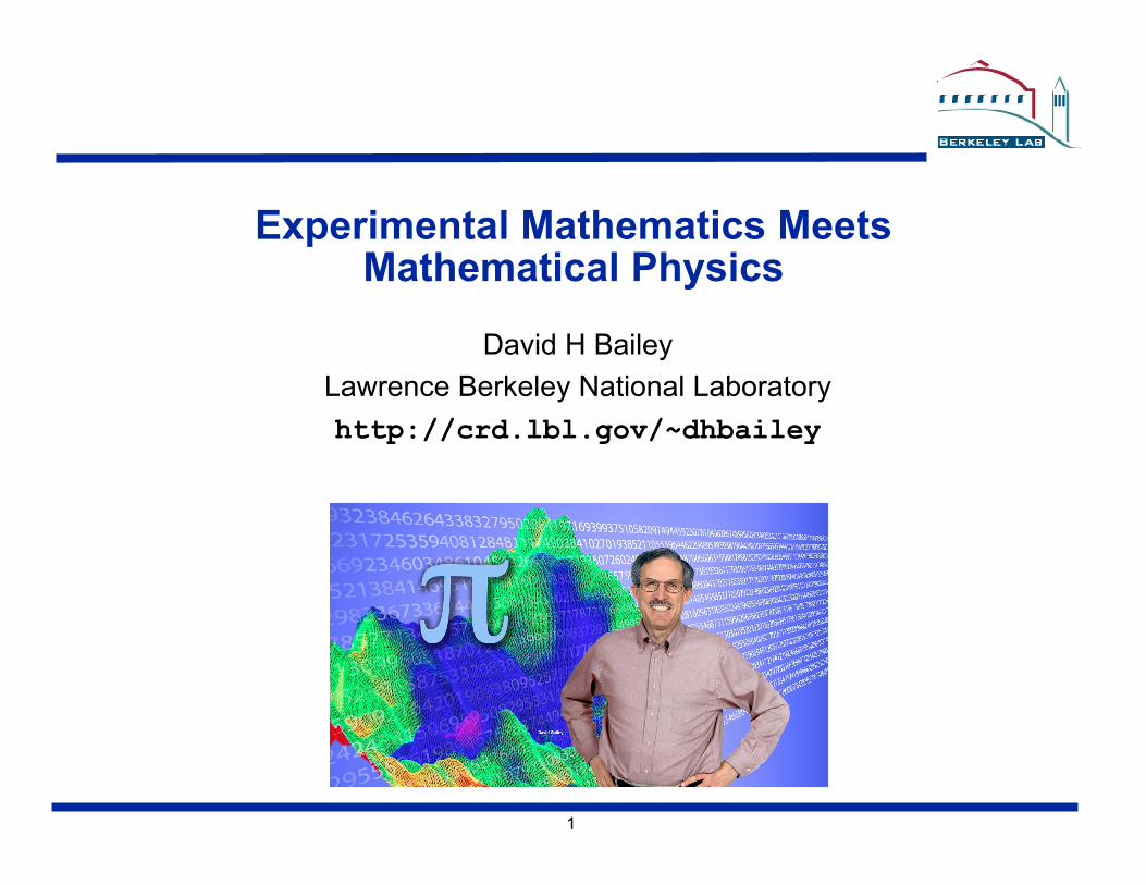
Experimental Mathematics Meets Mathematical Physics
David H Bailey Lawrence Berkeley National Laboratory http://crd.lbl.gov/~dhbailey
2
Applications of High-Precision Arithmetic in Modern Scientific Computing
Highly nonlinear computations. Computations involving highly ill-conditioned linear systems. Computations involving data with very large dynamic range. Large computations on highly parallel computer systems. Computations where numerical sensitivity is not currently a major
problem, but periodic testing is needed to ensure that results are reliable. Research problems in mathematics and mathematical physics that
involve constant recognition and integer relation detection.
Few physicists, chemists or engineers are highly expert in numerical analysis. Thus high-precision arithmetic is often a better remedy for severe numerical round-off error, even if the error could, in principle, be improved with more advanced algorithms or coding techniques.
3
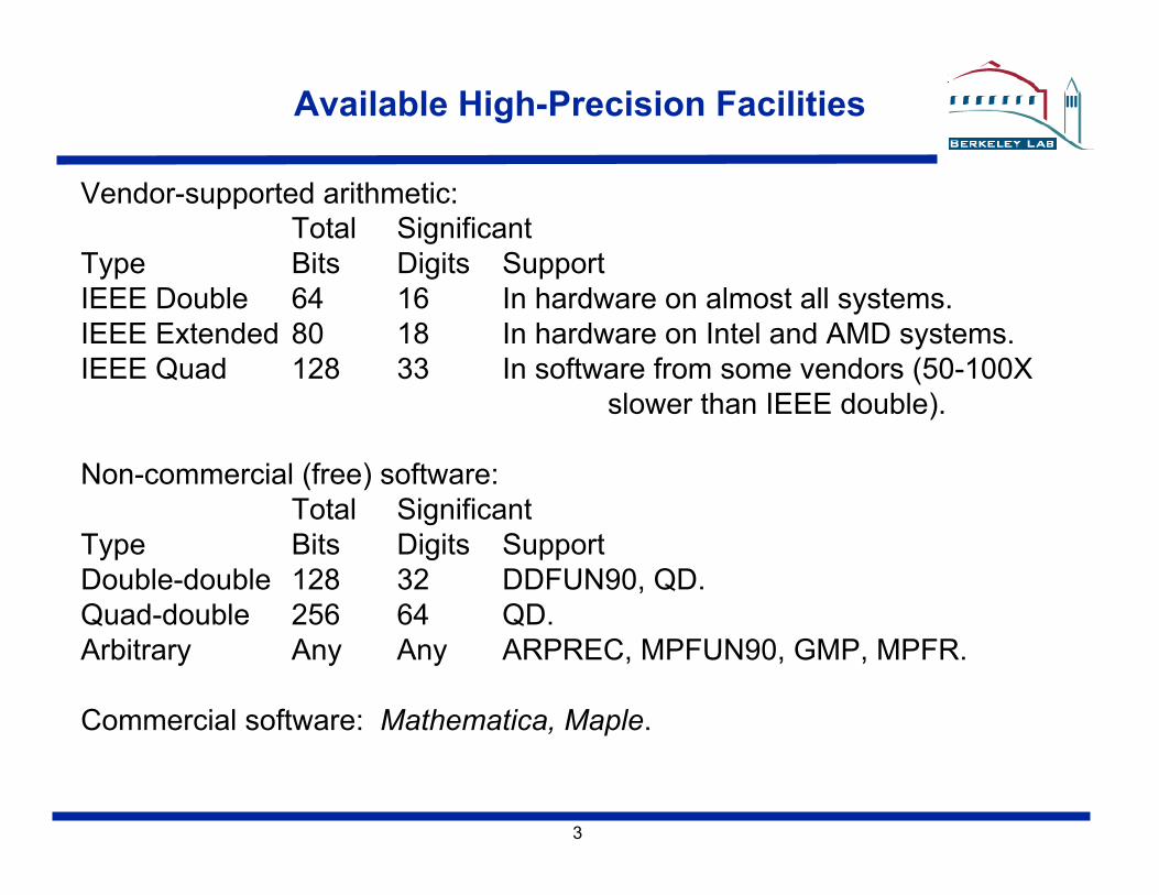
Available High-Precision Facilities
Vendor-supported arithmetic: Total Significant
Type Bits Digits Support IEEE Double 64 16 In hardware on almost all systems. IEEE Extended 80 18 In hardware on Intel and AMD systems. IEEE Quad 128 33 In software from some vendors (50-100X
slower than IEEE double).
Non-commercial (free) software: Total Significant
Type Bits Digits Support Double-double 128 32 DDFUN90, QD. Quad-double 256 64 QD. Arbitrary Any Any ARPREC, MPFUN90, GMP, MPFR.
Commercial software: Mathematica, Maple.
4
LBNL’s High-Precision Software
QD: double-double (31 digits) and quad-double (62 digits). ARPREC: arbitrary precision. Low-level routines written in C++. C++ and Fortran-90 translation modules permit use with existing C++ and
Fortran-90 programs -- only minor code changes are required. Includes many common functions: sqrt, cos, exp, gamma, etc. PSLQ, root finding, numerical integration.
Available at: http://www.experimentalmath.info
Authors: Xiaoye Li, Yozo Hida, Brandon Thompson and DHB
5
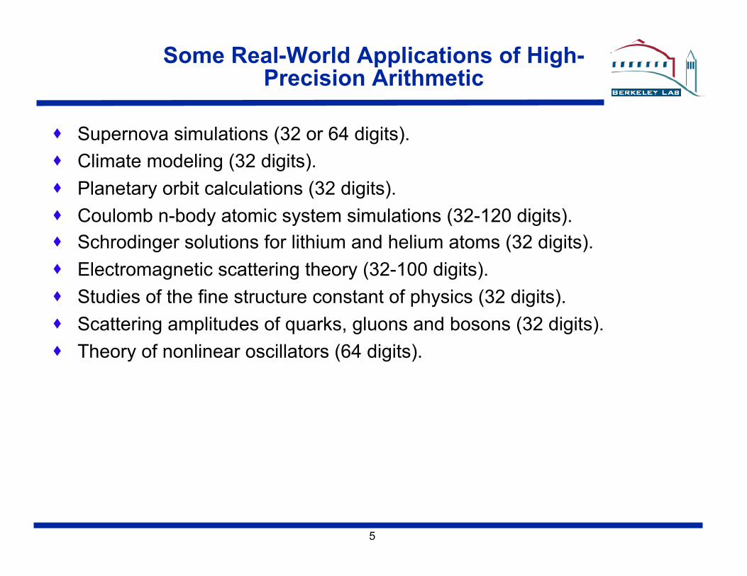
Some Real-World Applications of High-Precision Arithmetic
Supernova simulations (32 or 64 digits). Climate modeling (32 digits). Planetary orbit calculations (32 digits). Coulomb n-body atomic system simulations (32-120 digits). Schrodinger solutions for lithium and helium atoms (32 digits). Electromagnetic scattering theory (32-100 digits). Studies of the fine structure constant of physics (32 digits). Scattering amplitudes of quarks, gluons and bosons (32 digits). Theory of nonlinear oscillators (64 digits).
6
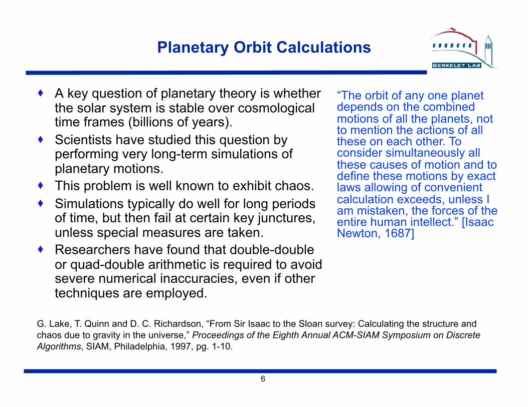
Planetary Orbit Calculations
A key question of planetary theory is whether the solar system is stable over cosmological time frames (billions of years).
Scientists have studied this question by performing very long-term simulations of planetary motions.
This problem is well known to exhibit chaos. Simulations typically do well for long periods
of time, but then fail at certain key junctures, unless special measures are taken.
Researchers have found that double-double or quad-double arithmetic is required to avoid severe numerical inaccuracies, even if other techniques are employed.
“The orbit of any one planet depends on the combined motions of all the planets, not to mention the actions of all these on each other. To consider simultaneously all these causes of motion and to define these motions by exact laws allowing of convenient calculation exceeds, unless I am mistaken, the forces of the entire human intellect.” [Isaac Newton, 1687]"
G. Lake, T. Quinn and D. C. Richardson, “From Sir Isaac to the Sloan survey: Calculating the structure and chaos due to gravity in the universe,” Proceedings of the Eighth Annual ACM-SIAM Symposium on Discrete Algorithms, SIAM, Philadelphia, 1997, pg. 1-10.
7
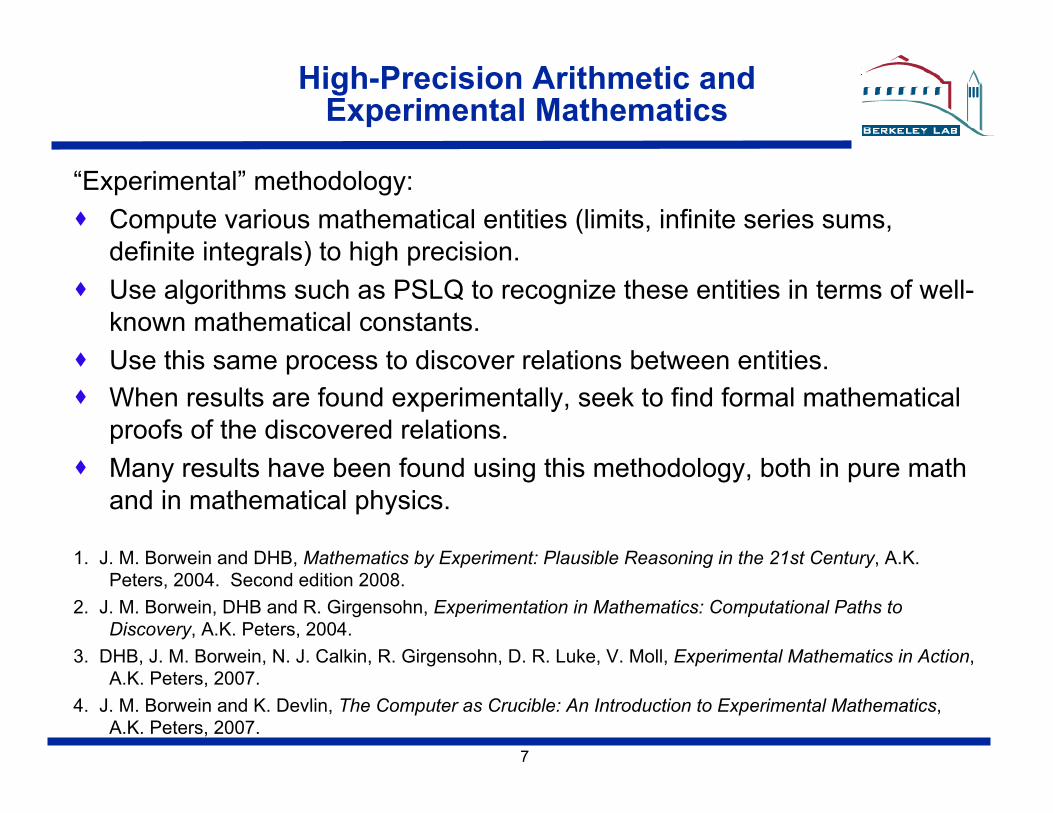
High-Precision Arithmetic and Experimental Mathematics
“Experimental” methodology: Compute various mathematical entities (limits, infinite series sums,
definite integrals) to high precision. Use algorithms such as PSLQ to recognize these entities in terms of well-
known mathematical constants. Use this same process to discover relations between entities. When results are found experimentally, seek to find formal mathematical
proofs of the discovered relations. Many results have been found using this methodology, both in pure math
and in mathematical physics.
1. J. M. Borwein and DHB, Mathematics by Experiment: Plausible Reasoning in the 21st Century, A.K. Peters, 2004. Second edition 2008.
2. J. M. Borwein, DHB and R. Girgensohn, Experimentation in Mathematics: Computational Paths to Discovery, A.K. Peters, 2004.
3. DHB, J. M. Borwein, N. J. Calkin, R. Girgensohn, D. R. Luke, V. Moll, Experimental Mathematics in Action, A.K. Peters, 2007.
4. J. M. Borwein and K. Devlin, The Computer as Crucible: An Introduction to Experimental Mathematics, A.K. Peters, 2007.
8
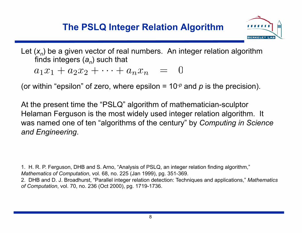
The PSLQ Integer Relation Algorithm
Let (xn) be a given vector of real numbers. An integer relation algorithm finds integers (an) such that
(or within “epsilon” of zero, where epsilon = 10-p and p is the precision).
At the present time the “PSLQ” algorithm of mathematician-sculptor Helaman Ferguson is the most widely used integer relation algorithm. It was named one of ten “algorithms of the century” by Computing in Science and Engineering.
1. H. R. P. Ferguson, DHB and S. Arno, “Analysis of PSLQ, an integer relation finding algorithm,” Mathematics of Computation, vol. 68, no. 225 (Jan 1999), pg. 351-369. 2. DHB and D. J. Broadhurst, “Parallel integer relation detection: Techniques and applications,” Mathematics of Computation, vol. 70, no. 236 (Oct 2000), pg. 1719-1736.
a1x1 + a2x2 + · · · + anxn = 0
9
PSLQ, Continued
PSLQ constructs a sequence of integer-valued matrices Bn that reduces the vector y = x Bn, until either the relation is found (as one of the columns of Bn), or else precision is exhausted.
At the same time, PSLQ generates a steadily growing bound on the size of any possible relation.
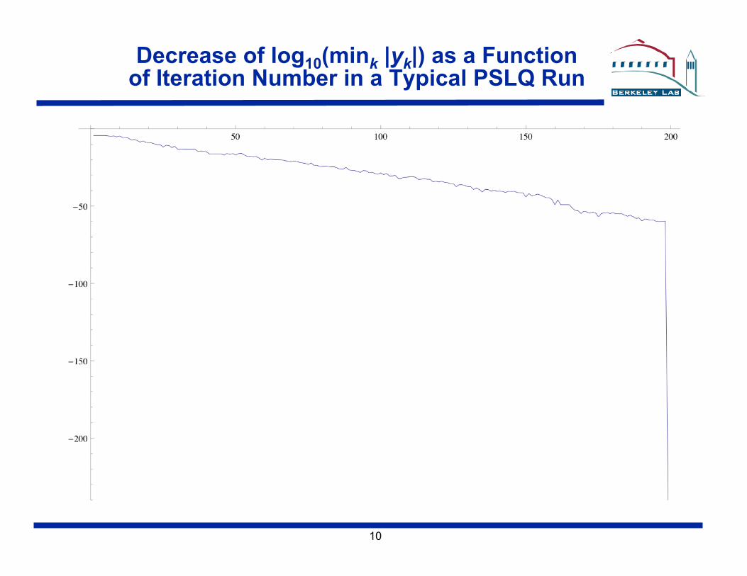
When a relation is found, the size of smallest entry of the vector y abruptly drops to roughly “epsilon” (i.e. 10-p, where p is the number of digits of precision).
The size of this drop can be viewed as a “confidence level” that the relation is real and not merely a numerical artifact -- a drop of 20+ orders of magnitude almost always indicates a real relation.
PSLQ (or any other integer relation scheme) requires very high precision arithmetic (at least nd digits, where d is the size in digits of the largest ak), both in the input data and in the operation of the algorithm.
10
Decrease of log10(mink |yk|) as a Function of Iteration Number in a Typical PSLQ Run
11
Methodology for Using PSLQ to Recognize An Unknown Constant α
Calculate α to high precision – typically 100 - 1000 digits. This is often the most computationally expensive part of the entire process.
Based on experience with similar constants or relations, make a list of possible terms on the right-hand side (RHS) of a linear formula for α, then calculate each of the n RHS terms to the same precision as α.
If you suspect α is algebraic of degree n (the root of a degree-n polynomial with integer coefficients), compute the vector (1, α, α2, α3, …, αn).
Apply PSLQ to the (n+1)-long vector, using the same numeric precision as α, but with a detection threshold a few orders of magnitude larger than “epsilon”– e.g., 10-480 instead of 10-500 for 500-digit arithmetic.
When PSLQ runs, look for a detection following a drop in the size of the reduced y vector by at least 20 orders of magnitude, to value near epsilon.
If no credible relation is found, try expanding the list of RHS terms. Another possibility is to search for multiplicative relations (i.e., monomial
expressions), which can be done by taking logarithms of α and constants.
12
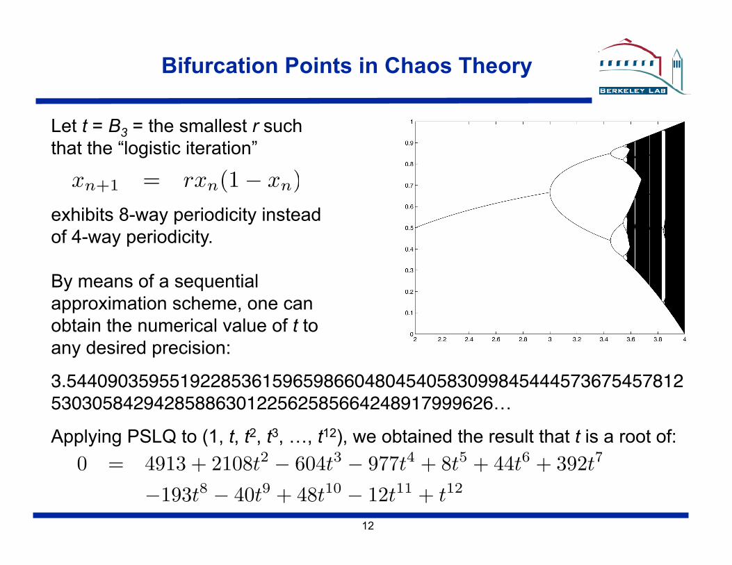
Bifurcation Points in Chaos Theory
exhibits 8-way periodicity instead of 4-way periodicity.
By means of a sequential approximation scheme, one can obtain the numerical value of t to any desired precision:
Let t = B3 = the smallest r such that the “logistic iteration”
3.5440903595519228536159659866048045405830998454445736754578125303058429428588630122562585664248917999626…
Applying PSLQ to (1, t, t2, t3, …, t12), we obtained the result that t is a root of:
xn+1 = rxn(1− xn)
0 = 4913 + 2108t2 − 604t3 − 977t4 + 8t5 + 44t6 + 392t7
−193t8 − 40t9 + 48t10 − 12t11 + t12
13
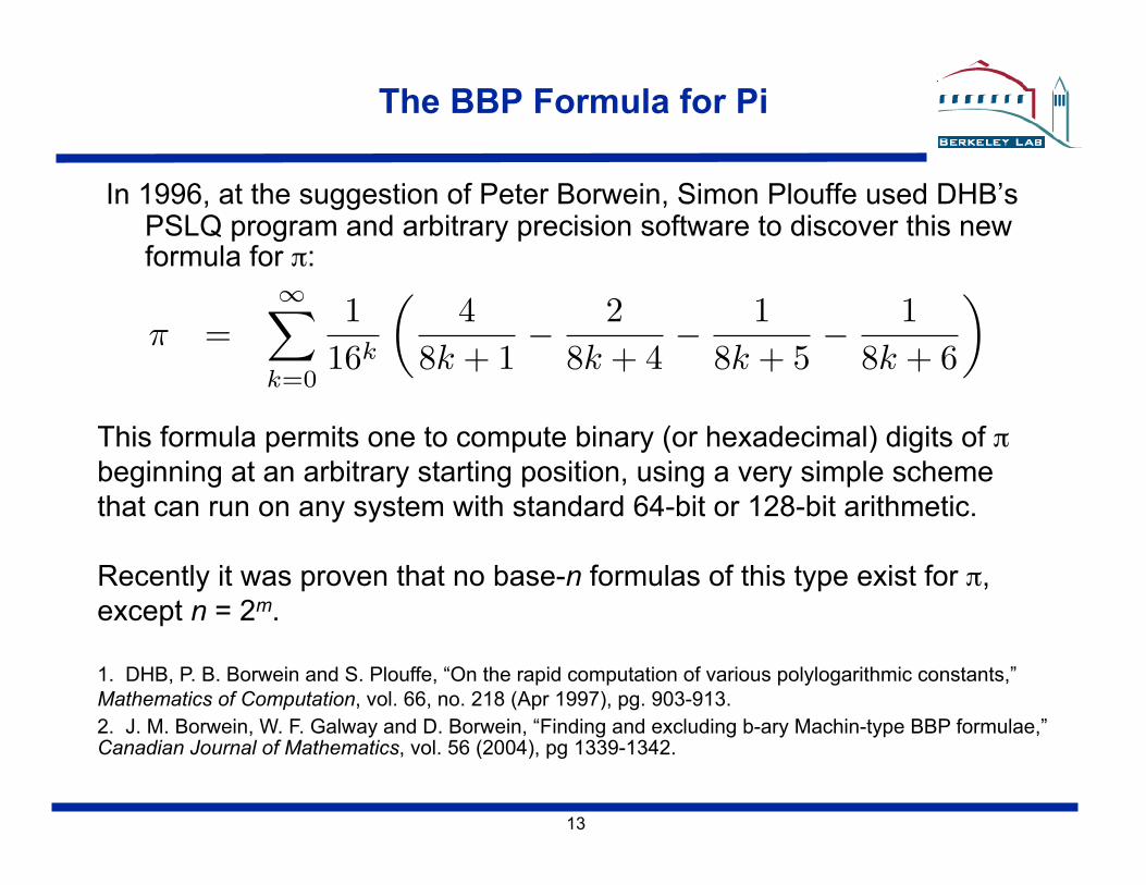
The BBP Formula for Pi
In 1996, at the suggestion of Peter Borwein, Simon Plouffe used DHB’s PSLQ program and arbitrary precision software to discover this new formula for π:
This formula permits one to compute binary (or hexadecimal) digits of π beginning at an arbitrary starting position, using a very simple scheme that can run on any system with standard 64-bit or 128-bit arithmetic.
Recently it was proven that no base-n formulas of this type exist for π, except n = 2m.
1. DHB, P. B. Borwein and S. Plouffe, “On the rapid computation of various polylogarithmic constants,” Mathematics of Computation, vol. 66, no. 218 (Apr 1997), pg. 903-913. 2. J. M. Borwein, W. F. Galway and D. Borwein, “Finding and excluding b-ary Machin-type BBP formulae,” Canadian Journal of Mathematics, vol. 56 (2004), pg 1339-1342.
π =∞�
k=0
116k
�4
8k + 1− 2
8k + 4− 1
8k + 5− 1
8k + 6
�
14
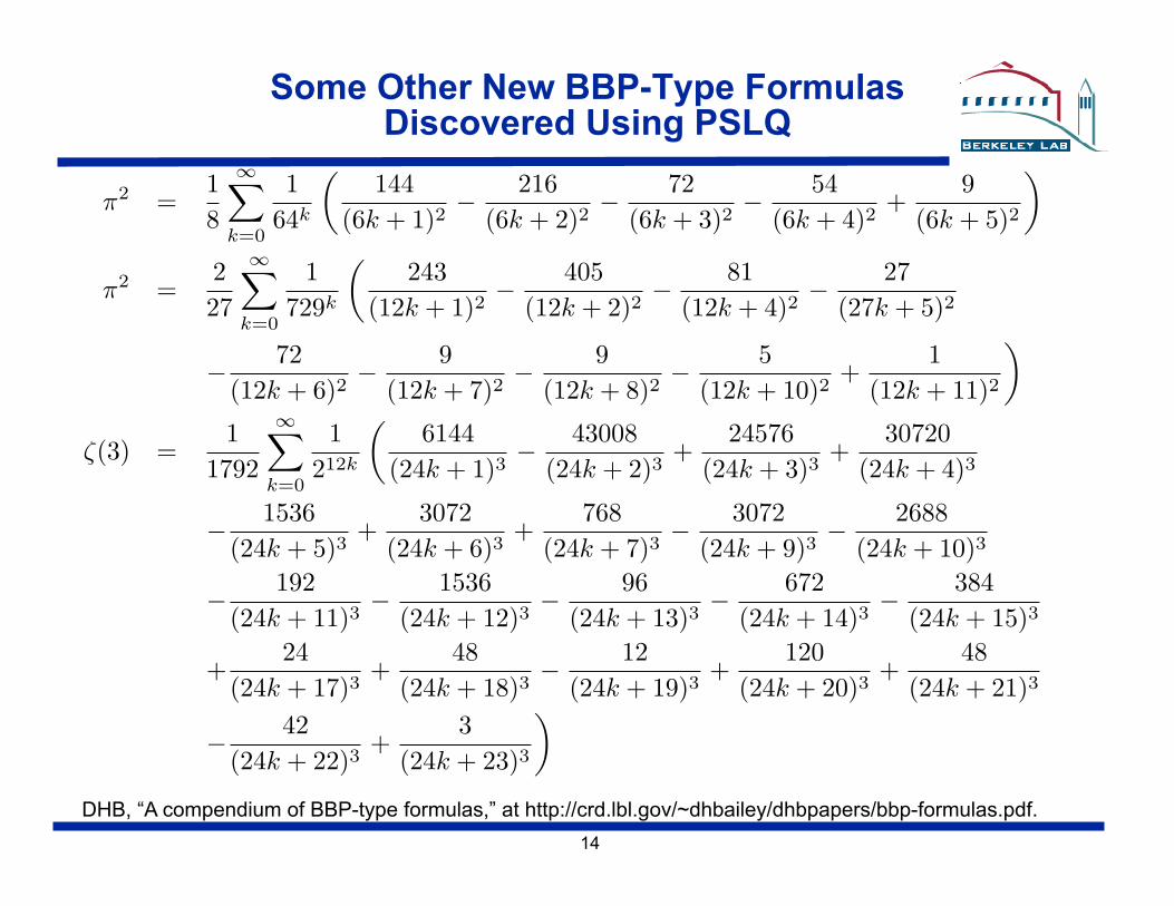
Some Other New BBP-Type Formulas Discovered Using PSLQ
π2 =18
∞�
k=0
164k
�144
(6k + 1)2− 216
(6k + 2)2− 72
(6k + 3)2− 54
(6k + 4)2+
9(6k + 5)2
�
π2 =227
∞�
k=0
1729k
�243
(12k + 1)2− 405
(12k + 2)2− 81
(12k + 4)2− 27
(27k + 5)2
− 72(12k + 6)2
− 9(12k + 7)2
− 9(12k + 8)2
− 5(12k + 10)2
+1
(12k + 11)2
�
ζ(3) =1
1792
∞�
k=0
1212k
�6144
(24k + 1)3− 43008
(24k + 2)3+
24576(24k + 3)3
+30720
(24k + 4)3
− 1536(24k + 5)3
+3072
(24k + 6)3+
768(24k + 7)3
− 3072(24k + 9)3
− 2688(24k + 10)3
− 192(24k + 11)3
− 1536(24k + 12)3
− 96(24k + 13)3
− 672(24k + 14)3
− 384(24k + 15)3
+24
(24k + 17)3+
48(24k + 18)3
− 12(24k + 19)3
+120
(24k + 20)3+
48(24k + 21)3
− 42(24k + 22)3
+3
(24k + 23)3
�
DHB, “A compendium of BBP-type formulas,” at http://crd.lbl.gov/~dhbailey/dhbpapers/bbp-formulas.pdf.
15
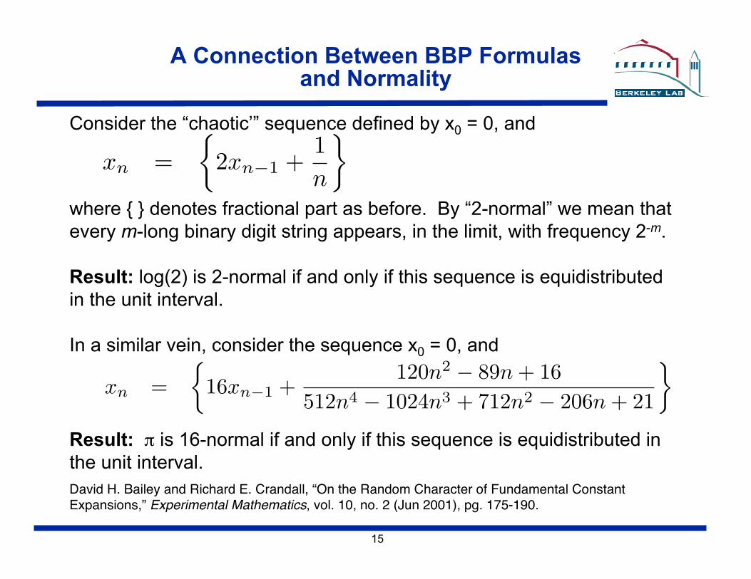
A Connection Between BBP Formulas and Normality
Consider the “chaotic’” sequence defined by x0 = 0, and
where { } denotes fractional part as before. By “2-normal” we mean that every m-long binary digit string appears, in the limit, with frequency 2-m.
Result: log(2) is 2-normal if and only if this sequence is equidistributed in the unit interval.
In a similar vein, consider the sequence x0 = 0, and
Result: π is 16-normal if and only if this sequence is equidistributed in the unit interval. David H. Bailey and Richard E. Crandall, “On the Random Character of Fundamental Constant Expansions,” Experimental Mathematics, vol. 10, no. 2 (Jun 2001), pg. 175-190.
xn =�
2xn−1 +1n
�
xn =�
16xn−1 +120n2 − 89n + 16
512n4 − 1024n3 + 712n2 − 206n + 21
�
16
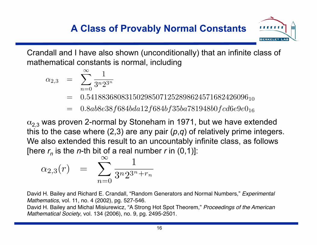
A Class of Provably Normal Constants
Crandall and I have also shown (unconditionally) that an infinite class of mathematical constants is normal, including
α2,3 was proven 2-normal by Stoneham in 1971, but we have extended this to the case where (2,3) are any pair (p,q) of relatively prime integers. We also extended this result to an uncountably infinite class, as follows [here rn is the n-th bit of a real number r in (0,1)]:
David H. Bailey and Richard E. Crandall, “Random Generators and Normal Numbers,” Experimental Mathematics, vol. 11, no. 4 (2002), pg. 527-546. "David H. Bailey and Michal Misiurewicz, “A Strong Hot Spot Theorem,” Proceedings of the American Mathematical Society, vol. 134 (2006), no. 9, pg. 2495-2501."
α2,3(r) =∞�
n=0
13n23n+rn
α2,3 =∞�
n=0
13n23n
= 0.54188368083150298507125289862457168242609610
= 0.8ab8e38f684bda12f684bf35ba781948b0fcd6e9e016
17
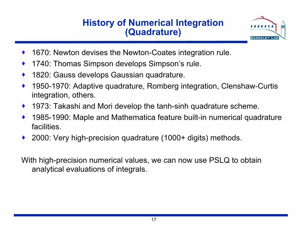
History of Numerical Integration (Quadrature)
1670: Newton devises the Newton-Coates integration rule. 1740: Thomas Simpson develops Simpson’s rule. 1820: Gauss develops Gaussian quadrature. 1950-1970: Adaptive quadrature, Romberg integration, Clenshaw-Curtis
integration, others. 1973: Takashi and Mori develop the tanh-sinh quadrature scheme. 1985-1990: Maple and Mathematica feature built-in numerical quadrature
facilities. 2000: Very high-precision quadrature (1000+ digits) methods.
With high-precision numerical values, we can now use PSLQ to obtain analytical evaluations of integrals.
18
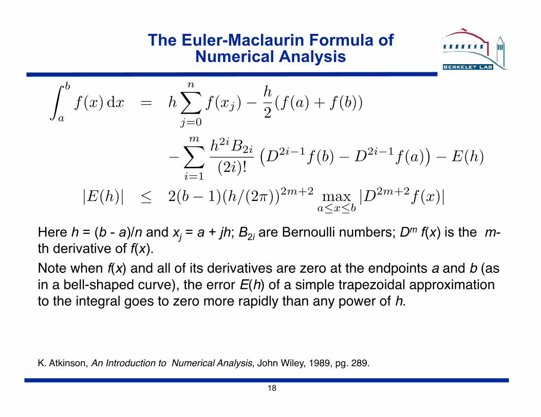
The Euler-Maclaurin Formula of Numerical Analysis
Here h = (b - a)/n and xj = a + jh; B2i are Bernoulli numbers; Dm f(x) is the m-th derivative of f(x). Note when f(x) and all of its derivatives are zero at the endpoints a and b (as in a bell-shaped curve), the error E(h) of a simple trapezoidal approximation to the integral goes to zero more rapidly than any power of h."
K. Atkinson, An Introduction to Numerical Analysis, John Wiley, 1989, pg. 289."
� b
af(x) dx = h
n�
j=0
f(xj)−h
2(f(a) + f(b))
−m�
i=1
h2iB2i
(2i)!�D2i−1f(b)−D2i−1f(a)
�− E(h)
|E(h)| ≤ 2(b− 1)(h/(2π))2m+2 maxa≤x≤b
|D2m+2f(x)|
19
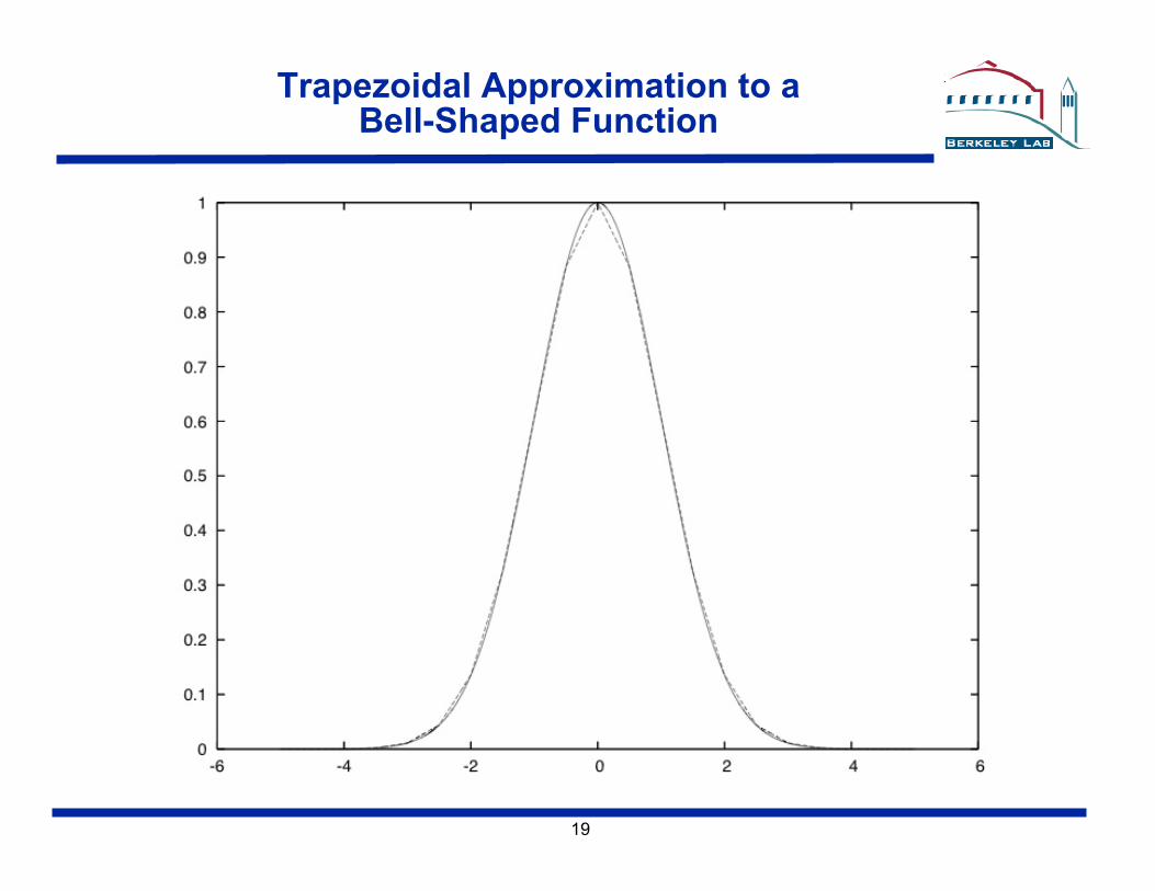
Trapezoidal Approximation to a Bell-Shaped Function
20
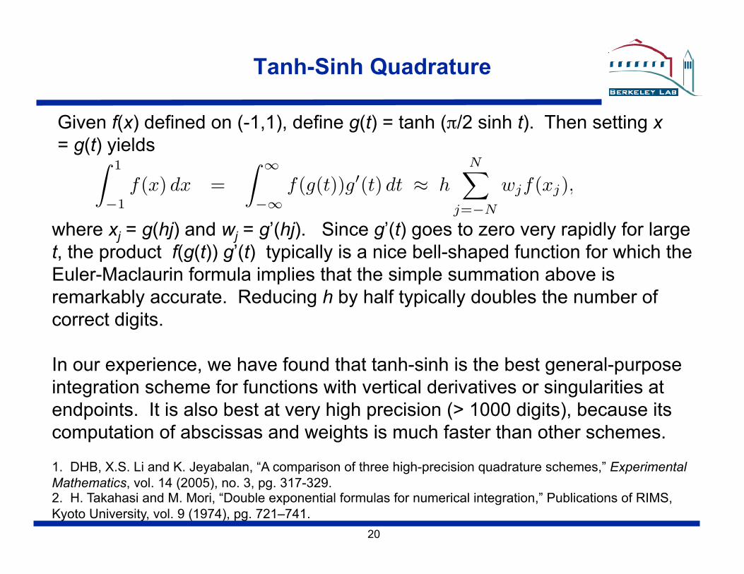
Tanh-Sinh Quadrature
Given f(x) defined on (-1,1), define g(t) = tanh (π/2 sinh t). Then setting x = g(t) yields
where xj = g(hj) and wj = g’(hj). Since g’(t) goes to zero very rapidly for large t, the product f(g(t)) g’(t) typically is a nice bell-shaped function for which the Euler-Maclaurin formula implies that the simple summation above is remarkably accurate. Reducing h by half typically doubles the number of correct digits.
In our experience, we have found that tanh-sinh is the best general-purpose integration scheme for functions with vertical derivatives or singularities at endpoints. It is also best at very high precision (> 1000 digits), because its computation of abscissas and weights is much faster than other schemes.
1. DHB, X.S. Li and K. Jeyabalan, “A comparison of three high-precision quadrature schemes,” Experimental Mathematics, vol. 14 (2005), no. 3, pg. 317-329. 2. H. Takahasi and M. Mori, “Double exponential formulas for numerical integration,” Publications of RIMS, Kyoto University, vol. 9 (1974), pg. 721–741.
� 1
−1f(x) dx =
� ∞
−∞f(g(t))g�(t) dt ≈ h
N�
j=−N
wjf(xj),
21
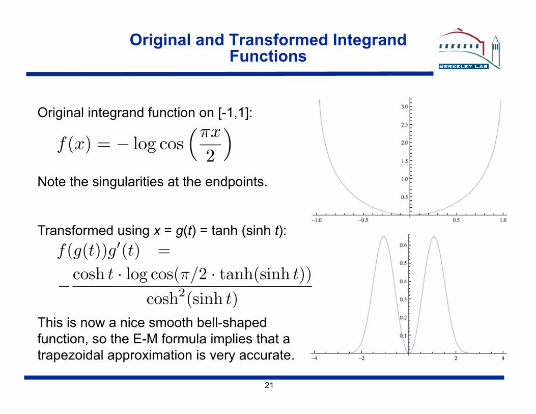
Original and Transformed Integrand Functions
Original integrand function on [-1,1]:
Note the singularities at the endpoints.
Transformed using x = g(t) = tanh (sinh t):
f(x) = − log cos�πx
2
�
This is now a nice smooth bell-shaped function, so the E-M formula implies that a trapezoidal approximation is very accurate.
f(g(t))g�(t) =
−cosh t · log cos(π/2 · tanh(sinh t))cosh2(sinh t)
22
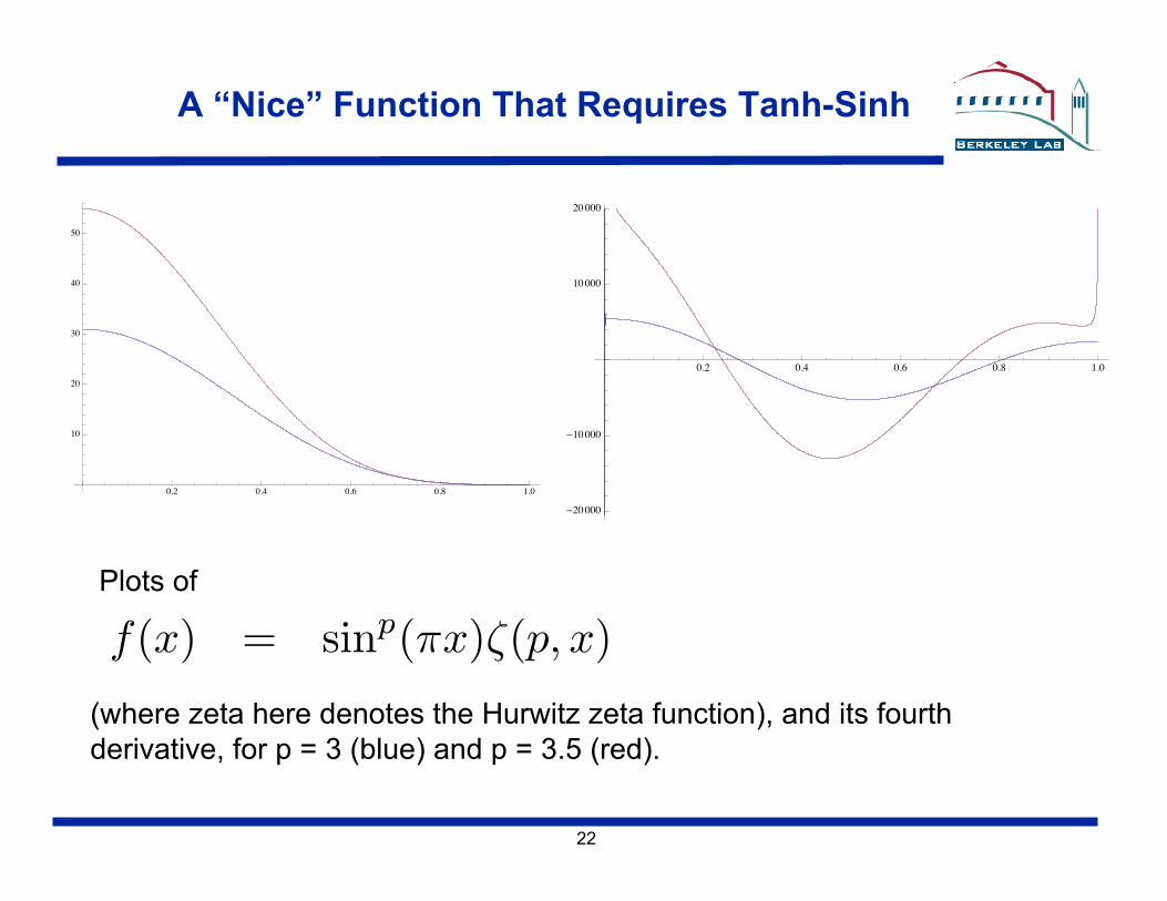
A “Nice” Function That Requires Tanh-Sinh
!"# !"$ !"% !"& '"!
'!
#!
(!
$!
)!
!"# !"$ !"% !"& '"!
!#!!!!
!'!!!!
'!!!!
#!!!!
Plots of
(where zeta here denotes the Hurwitz zeta function), and its fourth derivative, for p = 3 (blue) and p = 3.5 (red).
f(x) = sinp(πx)ζ(p, x)
23
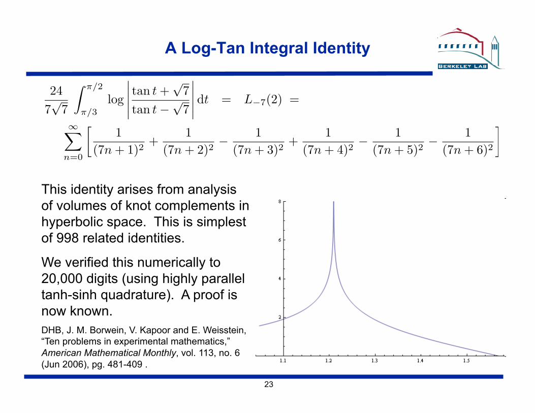
A Log-Tan Integral Identity
This identity arises from analysis of volumes of knot complements in hyperbolic space. This is simplest of 998 related identities.
We verified this numerically to 20,000 digits (using highly parallel tanh-sinh quadrature). A proof is now known. DHB, J. M. Borwein, V. Kapoor and E. Weisstein, “Ten problems in experimental mathematics,” American Mathematical Monthly, vol. 113, no. 6 (Jun 2006), pg. 481-409 .
247√
7
� π/2
π/3log
�����tan t +
√7
tan t−√
7
����� dt = L−7(2) =
∞�
n=0
�1
(7n + 1)2+
1(7n + 2)2
− 1(7n + 3)2
+1
(7n + 4)2− 1
(7n + 5)2− 1
(7n + 6)2
�
24
Computing High-Precision Values of Multi-Dimension Integrals
Computing multi-hundred digit numerical values of 2-D, 3-D and higher-dimensional integrals remains a major challenge.
Typical approach: Consider the 2-D or 3-D domain divided into 1-D lines. Use Gaussian quadrature (for regular functions) or tanh-sinh quadrature
(if function has vertical derivates or singularities on boundaries) on each of the 1-D lines.
Discontinue evaluation beyond points where it is clear that function-weight products are smaller than the “epsilon” of the precision level (this works better with tanh-sinh).
Even with “smart” evaluation that avoids unnecessary evaluations, the computational cost increases very sharply with dimension:
If 1000 evaluation points are required in 1-D for a given precision, then typically 1,000,000 are required in 2-D and 1,000,000,000 in 3-D, etc.
25
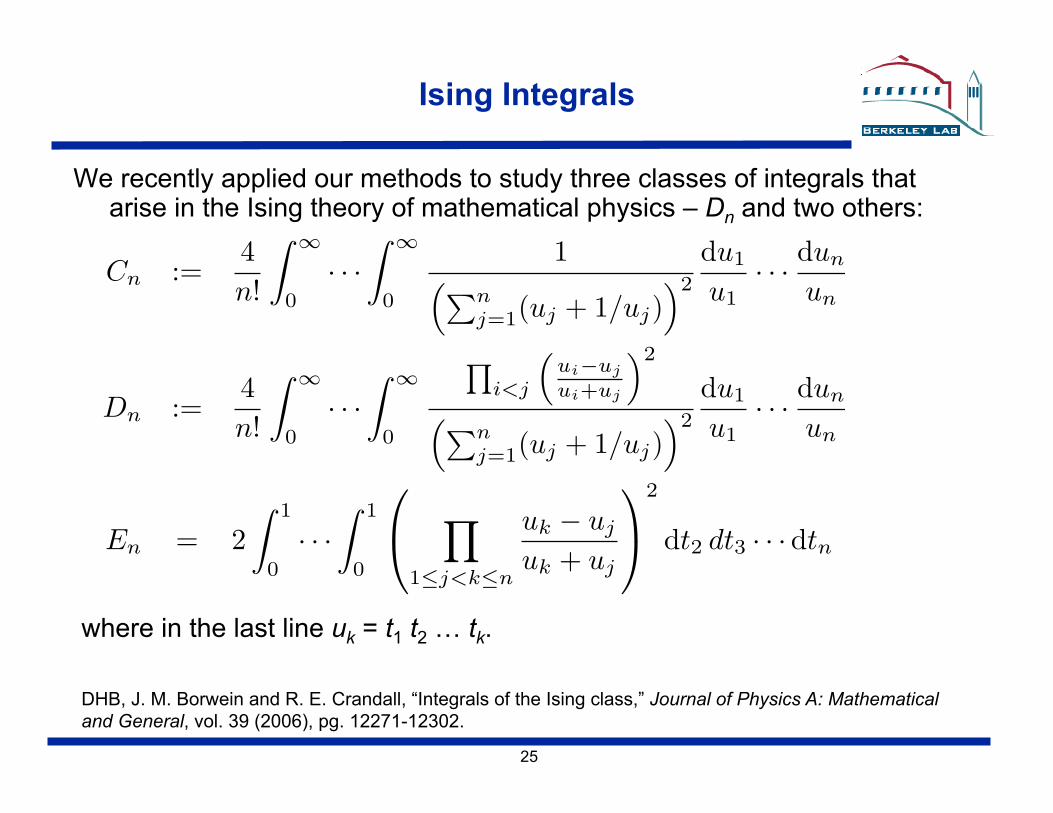
Ising Integrals
We recently applied our methods to study three classes of integrals that arise in the Ising theory of mathematical physics – Dn and two others:
where in the last line uk = t1 t2 … tk.
DHB, J. M. Borwein and R. E. Crandall, “Integrals of the Ising class,” Journal of Physics A: Mathematical and General, vol. 39 (2006), pg. 12271-12302.
Cn :=4n!
� ∞
0· · ·
� ∞
0
1��n
j=1(uj + 1/uj)�2
du1
u1· · · dun
un
Dn :=4n!
� ∞
0· · ·
� ∞
0
�i<j
�ui−uj
ui+uj
�2
��nj=1(uj + 1/uj)
�2
du1
u1· · · dun
un
En = 2� 1
0· · ·
� 1
0
�
1≤j<k≤n
uk − uj
uk + uj
2
dt2 dt3 · · · dtn
26
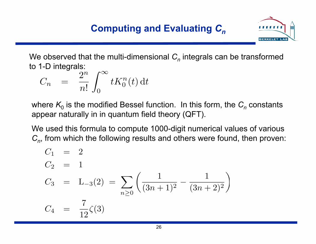
Computing and Evaluating Cn
where K0 is the modified Bessel function. In this form, the Cn constants appear naturally in in quantum field theory (QFT).
We used this formula to compute 1000-digit numerical values of various Cn, from which the following results and others were found, then proven:
We observed that the multi-dimensional Cn integrals can be transformed to 1-D integrals:
C1 = 2C2 = 1
C3 = L−3(2) =�
n≥0
�1
(3n + 1)2− 1
(3n + 2)2
�
C4 =712
ζ(3)
Cn =2n
n!
� ∞
0tKn
0 (t) dt
27
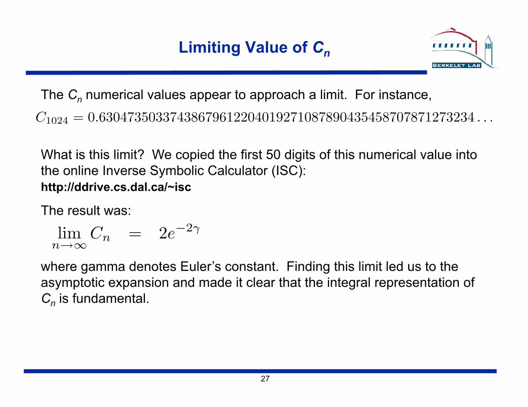
Limiting Value of Cn
The Cn numerical values appear to approach a limit. For instance,
What is this limit? We copied the first 50 digits of this numerical value into the online Inverse Symbolic Calculator (ISC): http://ddrive.cs.dal.ca/~isc
The result was:
where gamma denotes Euler’s constant. Finding this limit led us to the asymptotic expansion and made it clear that the integral representation of Cn is fundamental.
C1024 = 0.63047350337438679612204019271087890435458707871273234 . . .
limn→∞
Cn = 2e−2γ
28
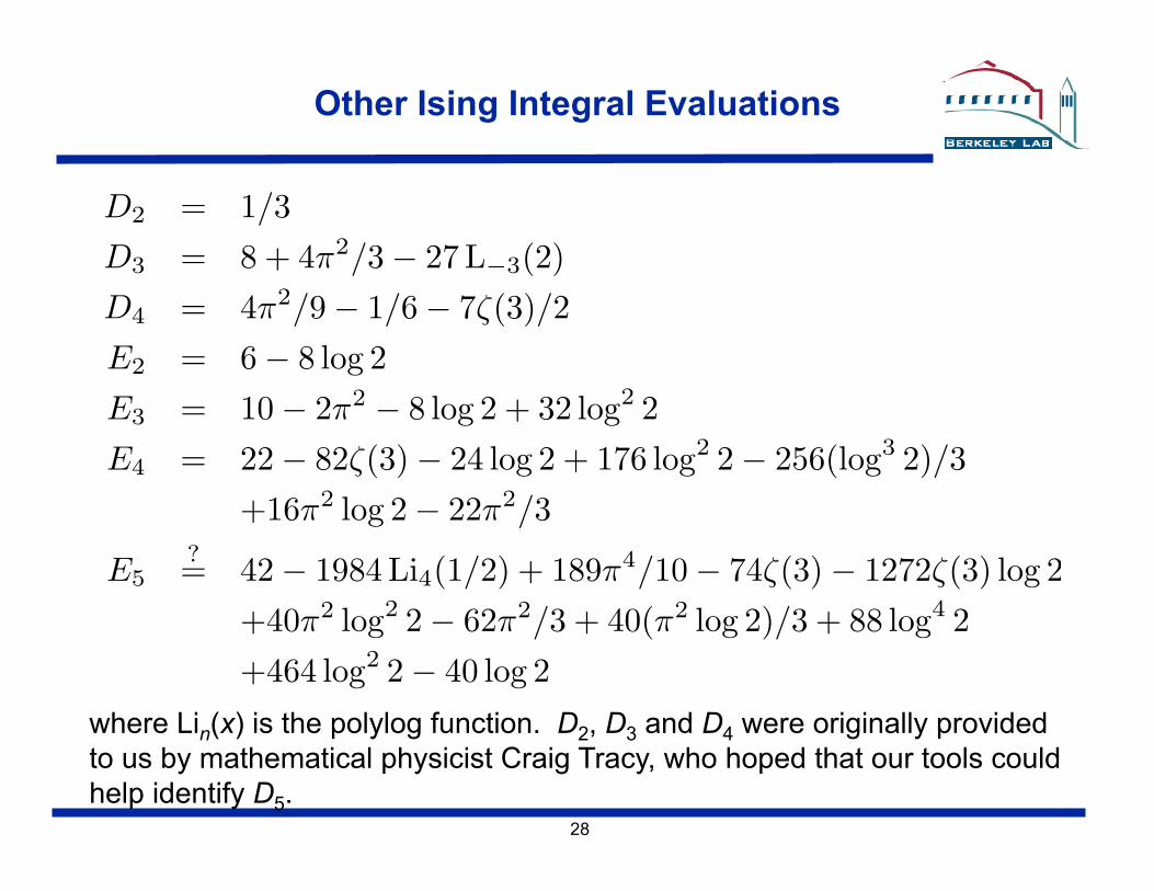
Other Ising Integral Evaluations
D2 = 1/3D3 = 8 + 4π2/3− 27 L−3(2)D4 = 4π2/9− 1/6− 7ζ(3)/2E2 = 6− 8 log 2E3 = 10− 2π2 − 8 log 2 + 32 log2 2E4 = 22− 82ζ(3)− 24 log 2 + 176 log2 2− 256(log3 2)/3
+16π2 log 2− 22π2/3
E5?= 42− 1984 Li4(1/2) + 189π4/10− 74ζ(3)− 1272ζ(3) log 2
+40π2 log2 2− 62π2/3 + 40(π2 log 2)/3 + 88 log4 2+464 log2 2− 40 log 2
where Lin(x) is the polylog function. D2, D3 and D4 were originally provided to us by mathematical physicist Craig Tracy, who hoped that our tools could help identify D5.
29
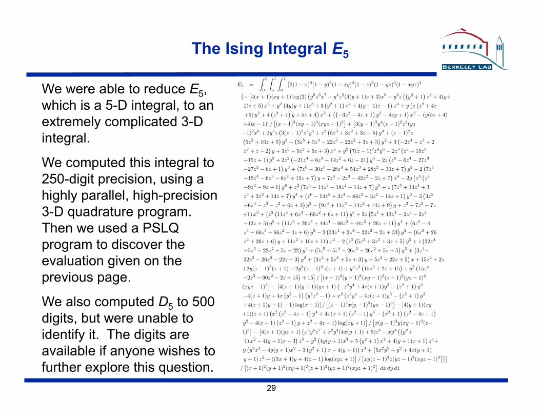
The Ising Integral E5
We were able to reduce E5, which is a 5-D integral, to an extremely complicated 3-D integral.
We computed this integral to 250-digit precision, using a highly parallel, high-precision 3-D quadrature program. Then we used a PSLQ program to discover the evaluation given on the previous page.
We also computed D5 to 500 digits, but were unable to identify it. The digits are available if anyone wishes to further explore this question.
E5 =� 1
0
� 1
0
� 1
0
�2(1− x)2(1− y)2(1− xy)2(1− z)2(1− yz)2(1− xyz)2
�−
�4(x + 1)(xy + 1) log(2)
�y5z3x7 − y4z2(4(y + 1)z + 3)x6 − y3z
��y2 + 1
�z2 + 4(y+
1)z + 5) x5 + y2�4y(y + 1)z3 + 3
�y2 + 1
�z2 + 4(y + 1)z − 1
�x4 + y
�z
�z2 + 4z
+5) y2 + 4�z2 + 1
�y + 5z + 4
�x3 +
��−3z2 − 4z + 1
�y2 − 4zy + 1
�x2 − (y(5z + 4)
+4)x− 1)] /�(x− 1)3(xy − 1)3(xyz − 1)3
�+
�3(y − 1)2y4(z − 1)2z2(yz
−1)2x6 + 2y3z�3(z − 1)2z3y5 + z2
�5z3 + 3z2 + 3z + 5
�y4 + (z − 1)2z
�5z2 + 16z + 5
�y3 +
�3z5 + 3z4 − 22z3 − 22z2 + 3z + 3
�y2 + 3
�−2z4 + z3 + 2
z2 + z − 2�y + 3z3 + 5z2 + 5z + 3
�x5 + y2
�7(z − 1)2z4y6 − 2z3
�z3 + 15z2
+15z + 1) y5 + 2z2�−21z4 + 6z3 + 14z2 + 6z − 21
�y4 − 2z
�z5 − 6z4 − 27z3
−27z2 − 6z + 1�y3 +
�7z6 − 30z5 + 28z4 + 54z3 + 28z2 − 30z + 7
�y2 − 2
�7z5
+15z4 − 6z3 − 6z2 + 15z + 7�y + 7z4 − 2z3 − 42z2 − 2z + 7
�x4 − 2y
�z3
�z3
−9z2 − 9z + 1�y6 + z2
�7z4 − 14z3 − 18z2 − 14z + 7
�y5 + z
�7z5 + 14z4 + 3
z3 + 3z2 + 14z + 7�y4 +
�z6 − 14z5 + 3z4 + 84z3 + 3z2 − 14z + 1
�y3 − 3
�3z5
+6z4 − z3 − z2 + 6z + 3�y2 −
�9z4 + 14z3 − 14z2 + 14z + 9
�y + z3 + 7z2 + 7z
+1)x3 +�z2
�11z4 + 6z3 − 66z2 + 6z + 11
�y6 + 2z
�5z5 + 13z4 − 2z3 − 2z2
+13z + 5) y5 +�11z6 + 26z5 + 44z4 − 66z3 + 44z2 + 26z + 11
�y4 +
�6z5 − 4
z4 − 66z3 − 66z2 − 4z + 6�y3 − 2
�33z4 + 2z3 − 22z2 + 2z + 33
�y2 +
�6z3 + 26
z2 + 26z + 6�y + 11z2 + 10z + 11
�x2 − 2
�z2
�5z3 + 3z2 + 3z + 5
�y5 + z
�22z4
+5z3 − 22z2 + 5z + 22�y4 +
�5z5 + 5z4 − 26z3 − 26z2 + 5z + 5
�y3 +
�3z4−
22z3 − 26z2 − 22z + 3�y2 +
�3z3 + 5z2 + 5z + 3
�y + 5z2 + 22z + 5
�x + 15z2 + 2z
+2y(z − 1)2(z + 1) + 2y3(z − 1)2z(z + 1) + y4z2�15z2 + 2z + 15
�+ y2
�15z4
−2z3 − 90z2 − 2z + 15�
+ 15�/
�(x− 1)2(y − 1)2(xy − 1)2(z − 1)2(yz − 1)2
(xyz − 1)2�−
�4(x + 1)(y + 1)(yz + 1)
�−z2y4 + 4z(z + 1)y3 +
�z2 + 1
�y2
−4(z + 1)y + 4x�y2 − 1
� �y2z2 − 1
�+ x2
�z2y4 − 4z(z + 1)y3 −
�z2 + 1
�y2
+4(z + 1)y + 1)− 1) log(x + 1)] /�(x− 1)3x(y − 1)3(yz − 1)3
�− [4(y + 1)(xy
+1)(z + 1)�x2
�z2 − 4z − 1
�y4 + 4x(x + 1)
�z2 − 1
�y3 −
�x2 + 1
� �z2 − 4z − 1
�
y2 − 4(x + 1)�z2 − 1
�y + z2 − 4z − 1
�log(xy + 1)
�/
�x(y − 1)3y(xy − 1)3(z−
1)3�−
�4(z + 1)(yz + 1)
�x3y5z7 + x2y4(4x(y + 1) + 5)z6 − xy3
��y2+
1) x2 − 4(y + 1)x− 3�z5 − y2
�4y(y + 1)x3 + 5
�y2 + 1
�x2 + 4(y + 1)x + 1
�z4+
y�y2x3 − 4y(y + 1)x2 − 3
�y2 + 1
�x− 4(y + 1)
�z3 +
�5x2y2 + y2 + 4x(y + 1)
y + 1) z2 + ((3x + 4)y + 4)z − 1�log(xyz + 1)
�/
�xy(z − 1)3z(yz − 1)3(xyz − 1)3
���
/�(x + 1)2(y + 1)2(xy + 1)2(z + 1)2(yz + 1)2(xyz + 1)2
�dx dy dz
30
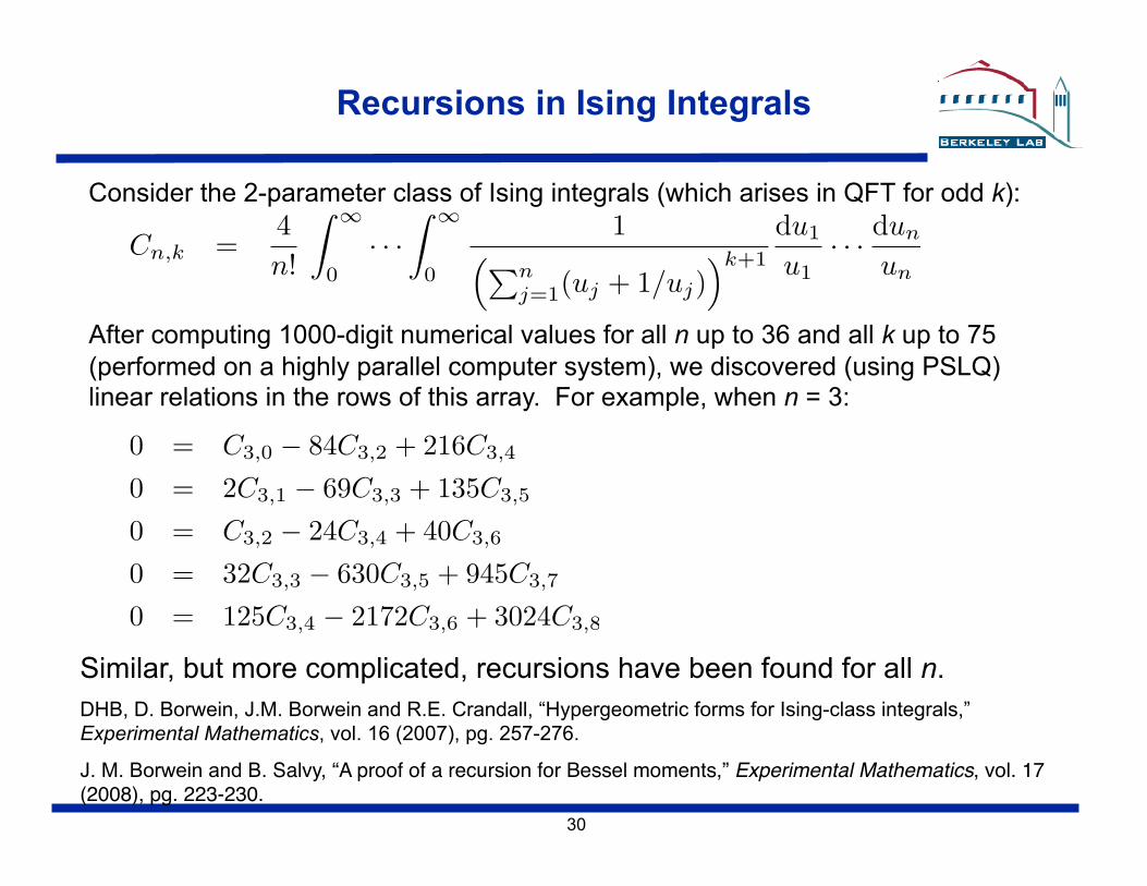
Recursions in Ising Integrals
Consider the 2-parameter class of Ising integrals (which arises in QFT for odd k):
After computing 1000-digit numerical values for all n up to 36 and all k up to 75 (performed on a highly parallel computer system), we discovered (using PSLQ) linear relations in the rows of this array. For example, when n = 3:
Similar, but more complicated, recursions have been found for all n. DHB, D. Borwein, J.M. Borwein and R.E. Crandall, “Hypergeometric forms for Ising-class integrals,” Experimental Mathematics, vol. 16 (2007), pg. 257-276.
J. M. Borwein and B. Salvy, “A proof of a recursion for Bessel moments,” Experimental Mathematics, vol. 17 (2008), pg. 223-230.
0 = C3,0 − 84C3,2 + 216C3,4
0 = 2C3,1 − 69C3,3 + 135C3,5
0 = C3,2 − 24C3,4 + 40C3,6
0 = 32C3,3 − 630C3,5 + 945C3,7
0 = 125C3,4 − 2172C3,6 + 3024C3,8
Cn,k =4n!
� ∞
0· · ·
� ∞
0
1��n
j=1(uj + 1/uj)�k+1
du1
u1· · · dun
un
31
Four Hypergeometric Evaluations
DHB, J.M. Borwein, D.M. Broadhurst and M.L. Glasser, “Elliptic integral representation of Bessel moments,” Journal of Physics A: Mathematical and Theoretical, vol. 41 (2008), 5203-5231."
c3,0 =3Γ6(1/3)32π22/3
=√
3π3
8 3F2
�1/2, 1/2, 1/2
1, 1
�����14
�
c3,2 =√
3π3
288 3F2
�1/2, 1/2, 1/2
2, 2
�����14
�
c4,0 =π4
4
∞�
n=0
�2nn
�4
44n=
π4
4 4F3
�1/2, 1/2, 1/2, 1/2
1, 1, 1
�����1�
c4,2 =π4
64
�44F3
�1/2, 1/2, 1/2, 1/2
1, 1, 1
�����1�
−34F3
�1/2, 1/2, 1/2, 1/2
2, 1, 1
�����1��− 3π2
16
32
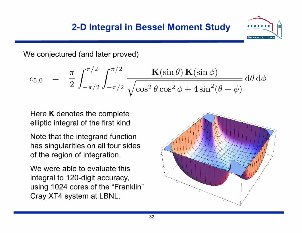
2-D Integral in Bessel Moment Study
We conjectured (and later proved)
Here K denotes the complete elliptic integral of the first kind
Note that the integrand function has singularities on all four sides of the region of integration.
We were able to evaluate this integral to 120-digit accuracy, using 1024 cores of the “Franklin” Cray XT4 system at LBNL.
c5,0 =π
2
� π/2
−π/2
� π/2
−π/2
K(sin θ)K(sinφ)�cos2 θ cos2 φ + 4 sin2(θ + φ)
dθ dφ
33
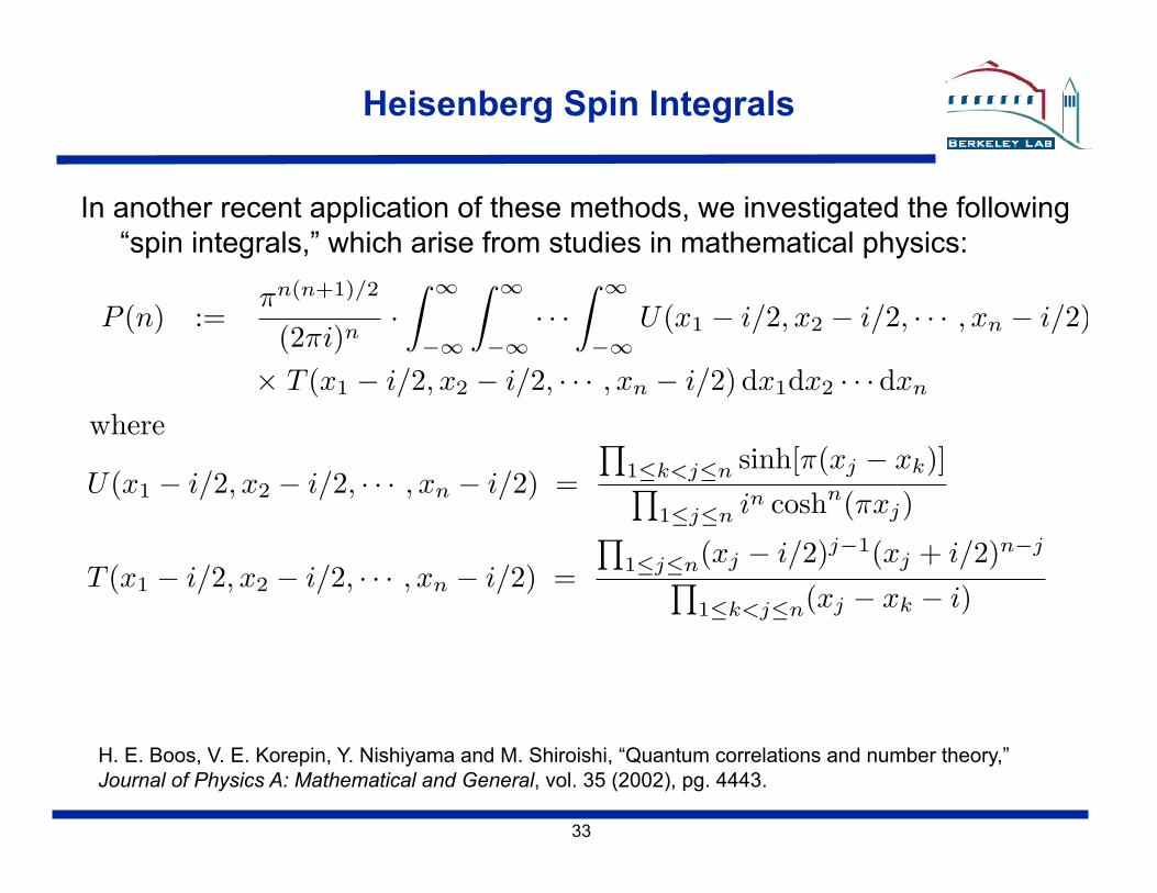
Heisenberg Spin Integrals
In another recent application of these methods, we investigated the following “spin integrals,” which arise from studies in mathematical physics:
H. E. Boos, V. E. Korepin, Y. Nishiyama and M. Shiroishi, “Quantum correlations and number theory,” Journal of Physics A: Mathematical and General, vol. 35 (2002), pg. 4443.
P (n) :=πn(n+1)/2
(2πi)n·� ∞
−∞
� ∞
−∞· · ·
� ∞
−∞U(x1 − i/2, x2 − i/2, · · · , xn − i/2)
× T (x1 − i/2, x2 − i/2, · · · , xn − i/2) dx1dx2 · · · dxn
where
U(x1 − i/2, x2 − i/2, · · · , xn − i/2) =�
1≤k<j≤n sinh[π(xj − xk)]�
1≤j≤n in coshn(πxj)
T (x1 − i/2, x2 − i/2, · · · , xn − i/2) =�
1≤j≤n(xj − i/2)j−1(xj + i/2)n−j
�1≤k<j≤n(xj − xk − i)
34
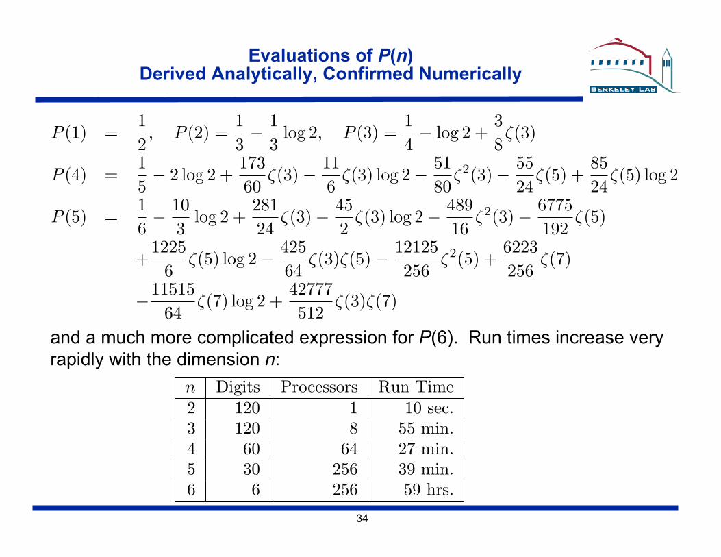
Evaluations of P(n) Derived Analytically, Confirmed Numerically
P (1) =12, P (2) =
13− 1
3log 2, P (3) =
14− log 2 +
38ζ(3)
P (4) =15− 2 log 2 +
17360
ζ(3)− 116
ζ(3) log 2− 5180
ζ2(3)− 5524
ζ(5) +8524
ζ(5) log 2
P (5) =16− 10
3log 2 +
28124
ζ(3)− 452
ζ(3) log 2− 48916
ζ2(3)− 6775192
ζ(5)
+1225
6ζ(5) log 2− 425
64ζ(3)ζ(5)− 12125
256ζ2(5) +
6223256
ζ(7)
−1151564
ζ(7) log 2 +42777512
ζ(3)ζ(7)
and a much more complicated expression for P(6). Run times increase very rapidly with the dimension n:
n Digits Processors Run Time2 120 1 10 sec.3 120 8 55 min.4 60 64 27 min.5 30 256 39 min.6 6 256 59 hrs.
35
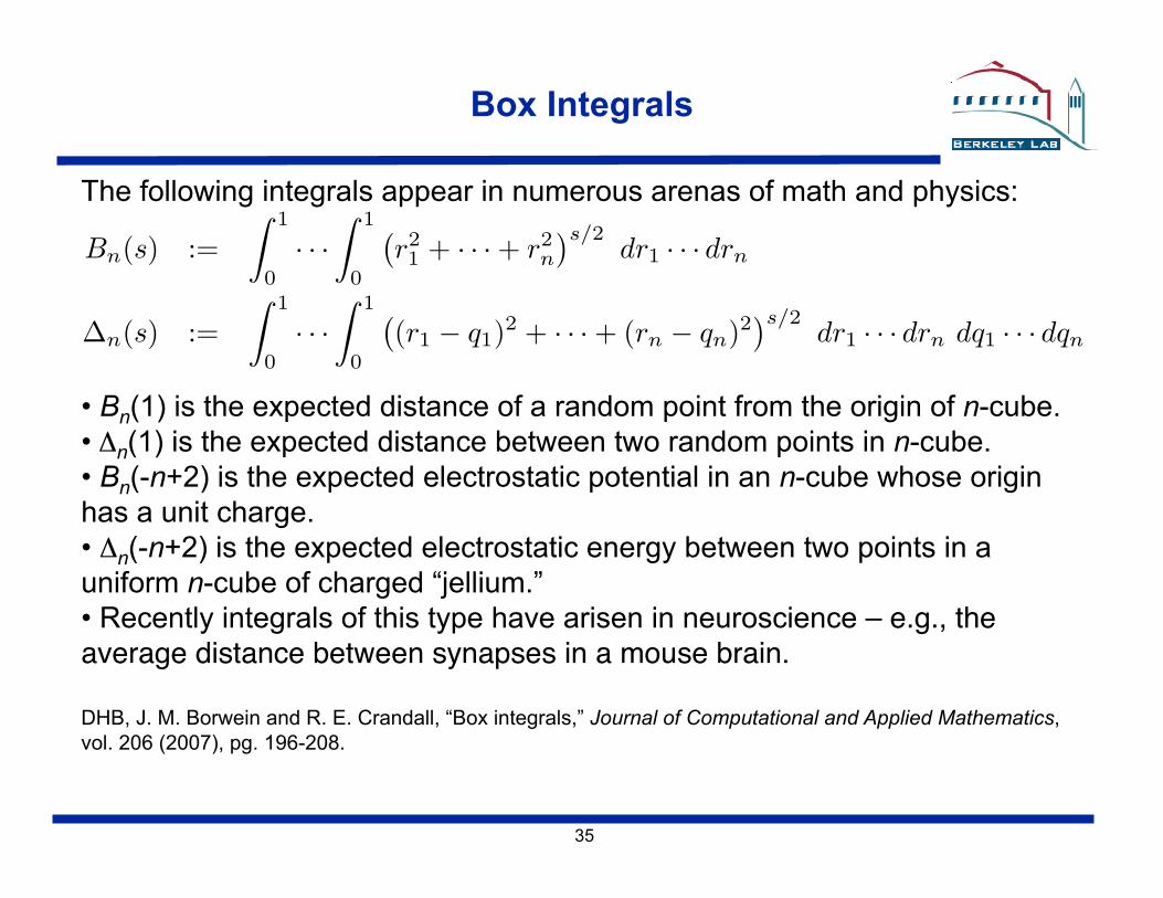
Box Integrals
The following integrals appear in numerous arenas of math and physics:
Bn(s) :=� 1
0· · ·
� 1
0
�r21 + · · · + r2
n
�s/2dr1 · · · drn
∆n(s) :=� 1
0· · ·
� 1
0
�(r1 − q1)2 + · · · + (rn − qn)2
�s/2dr1 · · · drn dq1 · · · dqn
• Bn(1) is the expected distance of a random point from the origin of n-cube. • Δn(1) is the expected distance between two random points in n-cube. • Bn(-n+2) is the expected electrostatic potential in an n-cube whose origin has a unit charge. • Δn(-n+2) is the expected electrostatic energy between two points in a uniform n-cube of charged “jellium.” • Recently integrals of this type have arisen in neuroscience – e.g., the average distance between synapses in a mouse brain. "
DHB, J. M. Borwein and R. E. Crandall, “Box integrals,” Journal of Computational and Applied Mathematics, vol. 206 (2007), pg. 196-208.
36
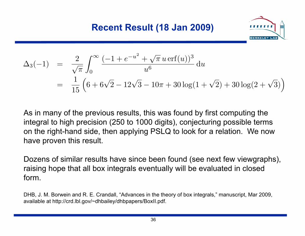
Recent Result (18 Jan 2009)
∆3(−1) =2√π
� ∞
0
(−1 + e−u2+√
π u erf(u))3
u6du
=115
�6 + 6
√2− 12
√3− 10π + 30 log(1 +
√2) + 30 log(2 +
√3)
�
As in many of the previous results, this was found by first computing the integral to high precision (250 to 1000 digits), conjecturing possible terms on the right-hand side, then applying PSLQ to look for a relation. We now have proven this result.
Dozens of similar results have since been found (see next few viewgraphs), raising hope that all box integrals eventually will be evaluated in closed form.
DHB, J. M. Borwein and R. E. Crandall, “Advances in the theory of box integrals,” manuscript, Mar 2009, available at http://crd.lbl.gov/~dhbailey/dhbpapers/BoxII.pdf.
37
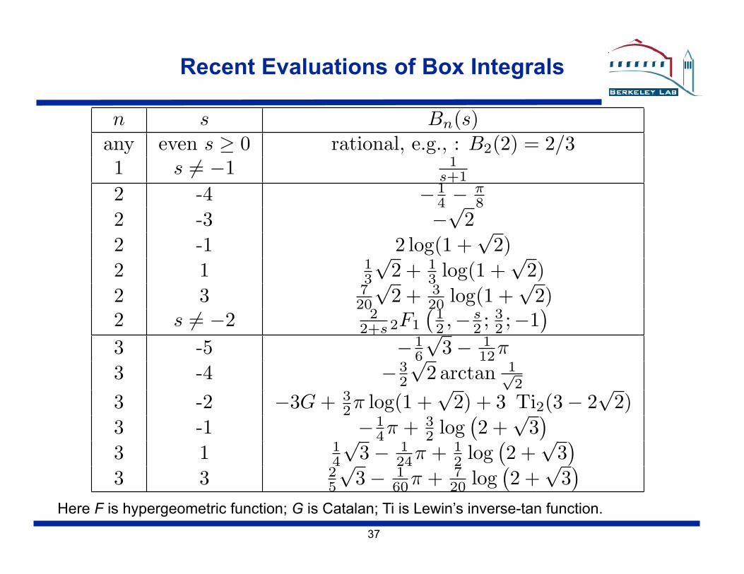
Recent Evaluations of Box Integrals
Here F is hypergeometric function; G is Catalan; Ti is Lewin’s inverse-tan function.
n s Bn(s)any even s ≥ 0 rational, e.g., : B2(2) = 2/31 s �= −1 1
s+1
2 -4 − 14 −
π8
2 -3 −√
22 -1 2 log(1 +
√2)
2 1 13
√2 + 1
3 log(1 +√
2)2 3 7
20
√2 + 3
20 log(1 +√
2)2 s �= −2 2
2+s 2F1
�12 ,− s
2 ; 32 ;−1
�
3 -5 − 16
√3− 1
12π3 -4 − 3
2
√2 arctan 1√
2
3 -2 −3G + 32π log(1 +
√2) + 3 Ti2(3− 2
√2)
3 -1 − 14π + 3
2 log�2 +
√3�
3 1 14
√3− 1
24π + 12 log
�2 +
√3�
3 3 25
√3− 1
60π + 720 log
�2 +
√3�
38
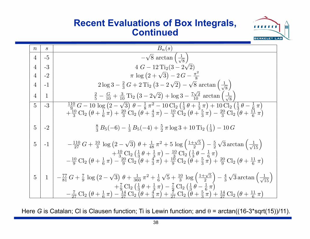
Recent Evaluations of Box Integrals, Continued
Here G is Catalan; Cl is Clausen function; Ti is Lewin function; and θ = arctan((16-3*sqrt(15))/11).
n s Bn(s)4 -5 −
√8 arctan
�1√8
�
4 -3 4 G− 12 Ti2(3− 2√
2)4 -2 π log
�2 +
√3�− 2 G− π2
8
4 -1 2 log 3− 23 G + 2 Ti2
�3− 2
√2�−√
8 arctan�
1√8
�
4 1 25 −
G10 + 3
10 Ti2�3− 2
√2�
+ log 3− 7√
210 arctan
�1√8
�
5 -3 1109 G− 10 log
�2−
√3�
θ − 18 π2 − 10 Cl2
�13 θ + 1
3 π�
+ 10 Cl2�
13 θ − 1
6 π�
+ 103 Cl2
�θ + 1
6 π�
+ 203 Cl2
�θ + 4
3 π�− 10
3 Cl2�θ + 5
3 π�− 20
3 Cl2�θ + 11
6 π�
5 -2 83 B5(−6)− 1
3 B5(−4) + 52 π log 3 + 10 Ti2
�13
�− 10 G
5 -1 − 11027 G + 10
3 log�2−
√3�
θ + 148 π2 + 5 log
�1+√
52
�− 5
2
√3 arctan
�1√15
�
+ 103 Cl2
�13 θ + 1
3 π�− 10
3 Cl2�
13 θ − 1
6 π�
− 109 Cl2
�θ + 1
6 π�− 20
9 Cl2�θ + 4
3 π�
+ 109 Cl2
�θ + 5
3 π�
+ 209 Cl2
�θ + 11
6 π�
5 1 − 7781 G + 7
9 log�2−
√3�
θ + 1360 π2 + 1
6
√5 + 10
3 log�
1+√
52
�− 4
3
√3 arctan
�1√15
�
+ 79 Cl2
�13 θ + 1
3 π�− 7
9 Cl2�
13 θ − 1
6 π�
− 727 Cl2
�θ + 1
6 π�− 14
27 Cl2�θ + 4
3 π�
+ 727 Cl2
�θ + 5
3 π�
+ 1427 Cl2
�θ + 11
6 π�
39
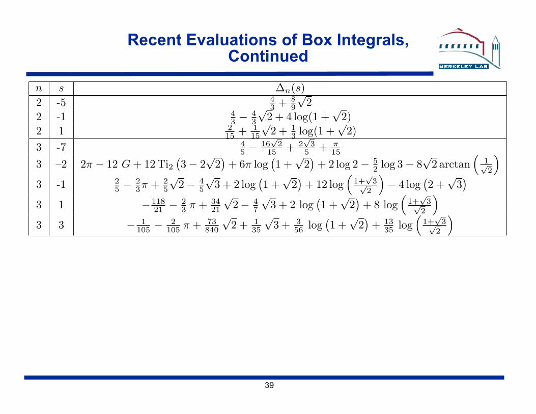
Recent Evaluations of Box Integrals, Continued
n s ∆n(s)2 -5 4
3 + 89
√2
2 -1 43 −
43
√2 + 4 log(1 +
√2)
2 1 215 + 1
15
√2 + 1
3 log(1 +√
2)3 -7 4
5 −16√
215 + 2
√3
5 + π15
3 –2 2π − 12 G + 12 Ti2�3− 2
√2�
+ 6π log�1 +
√2�
+ 2 log 2− 52 log 3− 8
√2 arctan
�1√2
�
3 -1 25 −
23π + 2
5
√2− 4
5
√3 + 2 log
�1 +
√2�
+ 12 log�
1+√
3√2
�− 4 log
�2 +
√3�
3 1 − 11821 −
23 π + 34
21
√2− 4
7
√3 + 2 log
�1 +
√2�
+ 8 log�
1+√
3√2
�
3 3 − 1105 −
2105 π + 73
840
√2 + 1
35
√3 + 3
56 log�1 +
√2�
+ 1335 log
�1+√
3√2
�
40
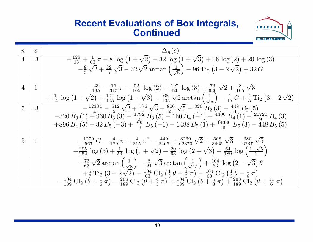
Recent Evaluations of Box Integrals, Continued
n s ∆n(s)4 -3 − 128
15 + 163 π − 8 log
�1 +
√2�− 32 log
�1 +
√3�
+ 16 log (2) + 20 log (3)− 8
5
√2 + 32
5
√3− 32
√2 arctan
�1√8
�− 96 Ti2
�3− 2
√2�
+ 32 G
4 1 − 23135 −
16315 π − 52
105 log (2) + 197420 log (3) + 73
630
√2 + 8
105
√3
+ 114 log
�1 +
√2�
+ 104105 log
�1 +
√3�− 68
105
√2 arctan
�1√8
�− 4
15 G + 45 Ti2
�3− 2
√2�
5 -3 − 1230463 − 512
21
√2 + 576
7
√3 + 800
21
√5− 320
3 B2 (3) + 4483 B2 (5)
−320 B3 (1) + 960 B3 (3)− 17923 B3 (5)− 160 B4 (−1) + 4400
3 B4 (1)− 207209 B4 (3)
+896B4 (5) + 32 B5 (−3) + 8003 B5 (−1)− 1488 B5 (1) + 14336
9 B5 (3)− 448 B5 (5)
5 1 − 1279567 G− 4
189 π + 4315 π2 − 449
3465 + 323962370
√2 + 568
3465
√3− 380
6237
√5
+ 295252 log (3) + 1
54 log�1 +
√2�
+ 2063 log
�2 +
√3�
+ 64189 log
�1+√
52
�
− 7363
√2 arctan
�1√8
�− 8
21
√3 arctan
�1√15
�+ 104
63 log�2−
√3�θ
+ 57 Ti2
�3− 2
√2�
+ 10463 Cl2
�13 θ + 1
3 π�− 104
63 Cl2�
13 θ − 1
6 π�
− 104189 Cl2
�θ + 1
6 π�− 208
189 Cl2�θ + 4
3 π�
+ 104189 Cl2
�θ + 5
3 π�
+ 208189 Cl2
�θ + 11
6 π�
41
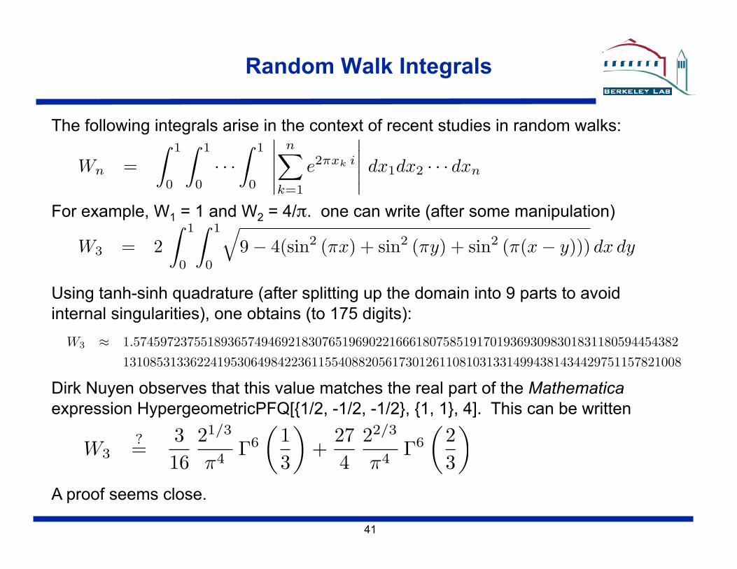
Random Walk Integrals
The following integrals arise in the context of recent studies in random walks:
For example, W1 = 1 and W2 = 4/π. one can write (after some manipulation)
Wn =� 1
0
� 1
0· · ·
� 1
0
�����
n�
k=1
e2πxk i
����� dx1dx2 · · · dxn
Using tanh-sinh quadrature (after splitting up the domain into 9 parts to avoid internal singularities), one obtains (to 175 digits):
W3 = 2� 1
0
� 1
0
�9− 4(sin2 (πx) + sin2 (πy) + sin2 (π(x− y))) dx dy
W3 ≈ 1.57459723755189365749469218307651969022166618075851917019369309830183118059445438213108531336224195306498422361155408820561730126110810313314994381434429751157821008
Dirk Nuyen observes that this value matches the real part of the Mathematica expression HypergeometricPFQ[{1/2, -1/2, -1/2}, {1, 1}, 4]. This can be written
A proof seems close.
W3?=
316
21/3
π4Γ6
�13
�+
274
22/3
π4Γ6
�23
�
42
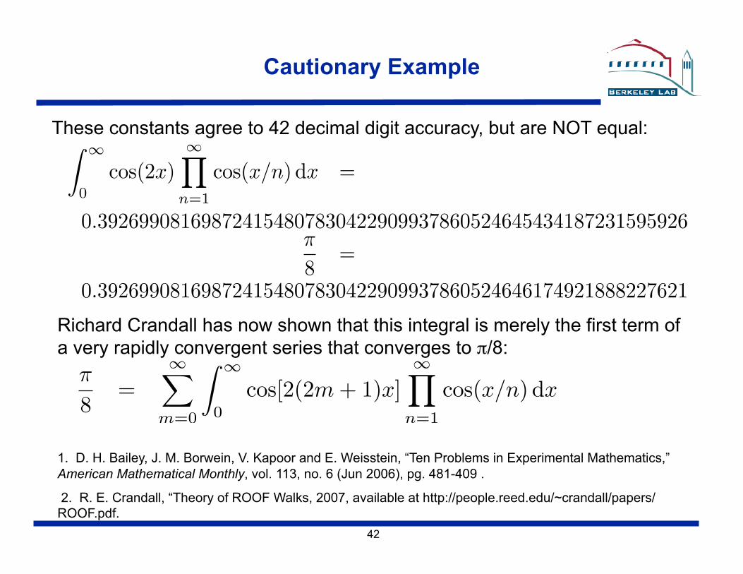
Cautionary Example
These constants agree to 42 decimal digit accuracy, but are NOT equal:
Richard Crandall has now shown that this integral is merely the first term of a very rapidly convergent series that converges to π/8:
1. D. H. Bailey, J. M. Borwein, V. Kapoor and E. Weisstein, “Ten Problems in Experimental Mathematics,” American Mathematical Monthly, vol. 113, no. 6 (Jun 2006), pg. 481-409 .
2. R. E. Crandall, “Theory of ROOF Walks, 2007, available at http://people.reed.edu/~crandall/papers/ROOF.pdf.
� ∞
0cos(2x)
∞�
n=1
cos(x/n) dx =
0.392699081698724154807830422909937860524645434187231595926π
8=
0.392699081698724154807830422909937860524646174921888227621
π
8=
∞�
m=0
� ∞
0cos[2(2m + 1)x]
∞�
n=1
cos(x/n) dx
43
Summary
Numerous state-of-the-art large-scale scientific calculations now require numerical precision beyond conventional 64-bit floating-point arithmetic.
The emerging “experimental” methodology in mathematics and mathematical physics often requires hundreds or even thousands of digits of precision.
Double-double, quad-double and arbitrary precision software libraries are now widely available (and in most cases are free). High-precision arithmetic is also integrated into Mathematica and Maple.
High-precision evaluation of integrals, followed by constant-recognition techniques, has been a particularly fruitful area of recent research, with many new results in pure math and mathematical physics.
There is a critical need to develop faster techniques for high-precision numerical integration in multiple dimensions.