experimental determination of the elastic coefficients of ...dschmitt/papers/experimental... ·...

GEOPHYSICS, VOL. 66, NO. 4 (JULY–AUGUST 2001); P. 1217–1225, 8 FIGS., 1 TABLE.

Experimental determination of the elastic coefficientsof an orthorhombic material

M. Mah∗ and D. R. Schmitt∗

ABSTRACT

In terms of elastic anisotropy, many rocks may be con-sidered to have orthorhombic symmetry. Experimentallydetermining the nine independent elastic coefficients re-quired for this case remains challenging. Elastic coeffi-cients are most often found from measurements of thephase velocity in a variety of directions throughout a ma-terial, but finding this plane-wave velocity is problematic.Here, quasi-P and quasi-Sphase speeds are found usingthe τ–p transformation through a composite material oforthorhombic symmetry. Arrays of specially constructedtransducers (0.65 MHz) with different modes of vibra-tion were placed on a rectangular prism of the material.More than 620 individual measures of phase speed wereobtained at different directions and subsequently usedin a generalized least-squares inversion that yields therequired elastic coefficients. The analysis does not ac-count for the effects of wave-speed dispersion evident inthe waveforms acquired in the composite material. Thisdispersion is particularly severe for the in-plane, quasi-S polarization and is possibly a consequence of the finelayered structure of the material.

INTRODUCTION

Wave velocity isotropy is the usual assumption in reflectionseismic profiling. However, most rocks are somewhat intrinsi-cally anisotropic because of mineralogical texture or alignedmicrocracks. Even simple consideration of this anisotropy im-proves the quality of seismic images (Okoye et al., 1996a). In-deed, neglecting to incorporate anisotropy during migrationcan introduce substantial errors when positioning of subsur-face reflectors (Claerbout, 1985). More realistic seismic imag-ing and modeling is hindered by the lack of understanding ofthe wave-speed anisotropy of many rocks. However, obtain-ing adequate information on rock anisotropy remains cumber-

Manuscript received by the Editor July 30, 1999; revised manuscript received October 30, 2000.∗University of Alberta, Institute for Geophysical Research, Department of Physics, Edmonton, Alberta T6G 2J1, Canada. E-mail: [email protected]; [email protected]© 2001 Society of Exploration Geophysicists. All rights reserved.

some, and any new methods that can ease acquisition of theappropriate information are welcome.

Kebaili and Schmitt (1997) develop an experimental methodwhere P-wave phase velocities are determined on both anisotropic and anisotropic material. Mah and Schmitt’s (2000)methodology expands to include the determination of S-wavevelocities on an isotropic glass block. We describe further de-velopment of an experimental method for measuring a suffi-cient number of both quasi-P and quasi-S phase velocities ina complex anisotropic media to allow the complete determi-nation of the set of elastic coefficients under the assumptionof orthorhombic symmetry. The method uses arrays of small,specially constructed transducers that impart and receive thequasi-P and two quasi-Smodes. Gathers of traces so obtainedare reminiscent of a walkaway vertical seismic profile (Kebailiand Schmitt, 1996) and may be analyzed in the τ–pdomain. Theadvantage of this procedure is that phase (plane-wave) veloc-ities, which are sometimes difficult to measure experimentallybut are necessary in characterizing a material’s elasticity, are di-rectly obtained. The inversion is tested on velocities measuredthrough an isotropic glass (Mah and Schmitt, 2000) and ananisotropic composite material. However, certain shear-wavearrivals suggest that in complex, layered materials, dispersionmay need to be considered.

PULSE TRANSMISSION AND ELASTICITY

Background

The intrinsic elastic stiffnesses of a rock are essential factorsneeded in describing anisotropy; in the most general case, 21independent coefficients are needed. Such a complete descrip-tion is difficult to achieve experimentally, however, and moststudies on rock presume that the rock is either isotropic, trans-versely isotropic (TI), or orthorhombic with 2, 5, and 9 indepen-dent constants, respectively (e.g., Musgrave, 1970). These elas-tic constants can be found in principle by measuring the staticdeformation of a test sample. However, quasi-static measure-ments can be subject to substantial error, ultrasonic pulse trans-mission methods are more popular in material characterization

1217

1218 Mah and Schmitt

(Markham, 1957). Briefly in review, one quasi-P wave and twoquasi-Splane waves propagate in any general direction througha homogeneous anisotropic medium obeying Hooke’s law (e.g.,Neighbours and Schacher, 1967):

σi j = ci jkl εkl , (1)

where σi j are the components of the stress, ci jkl are the elasticstiffness constants, and εkl are the components of the strain.[The nomenclature used here is the same as that of Musgrave(1970).]

If these are plane waves, the phase velocities and polarizationdirections are the eigenvalues and eigenvectors of

0i l Al = ρν2 Ai , (2)

where Al and Ai are the amplitudes, ρ is the density, ν is thephase velocity, and 0i l are the Christoffel symbols that dependon the elastic constants via

0i l = ci jkl n j nk. (3)

Here, nj and nk are the directional cosines.When the elastic coefficients are known, the wave-speeds

in any direction are determined by solving equation (2). Con-versely, the elastic coefficients can be determined by measuringa sufficient number of wave speeds. If the material is knownto be isotropic, the elastic coefficients are found by measuringonly a P- and an S-wave speed in any direction. The minimumnumber of wave-speed measurements required increases formaterials of lower symmetry (more independent coefficients)and if the directions of symmetry in a given test piece are un-known.

Since the early measurements of Markham (1957) on cu-bic and hexagonal metals, numerous methods have been de-veloped for geophysical application. A few methods includepulse transmission through specially machined spheres (Prosand Babuska, 1967; Thill et al., 1969; Pros and Podrouzkova,1974; Vestrum, 1994) or multifaceted prisms (Markham, 1957;Carlson et al., 1984; Arts et al., 1991; Cheadle et al., 1991;Vestrum, 1994) but most commonly are through carefully ori-ented cylindrical core samples (e.g., Kaarsberg, 1959; Vernikand Nur, 1992; Vernik, 1993; Johnston and Christensen, 1995;Hornby, 1996).

One complication in such analyses is that the phase, orplane-wave, velocity necessary to determine the elastic coef-ficient may often differ from the more easily obtained group(or ray) velocity. The physical consequences of this differenceare well documented (e.g., Musgrave, 1970; Auld, 1973) andintroduce ambiguity to experimental velocity measurementsin anisotropic media (Dellinger and Vernik, 1994; Vestrum,1994; Kebaili and Schmitt, 1997). Without careful considera-tion of the sample and transducer geometries, it can be difficultto know whether group, phase, or some intermediate value ismeasured. Group velocities may be converted to phase veloci-ties if a sufficient number of the former are measured to allowa smooth differentiation with respect to the propagation an-gle (see Thomsen, 1986). Indeed, Vestrum (1994) develops aspecialized procedure to invert the group velocities obtainedin pulse transmission experiments over a sphere and a mul-tifaceted prism of an orthorhombic composite similar to thatused here. Okoye et al. (1996b) resort to smooth polynomial

fitting of phase velocities observed through a bar of TI materialto minimize the errors.

Not being able to measure phase velocities as describedin equation (2) adds error to or substantially complicatesthe determination of the elastic coefficients in pulse trans-mission measurements (Vestrum, 1994; Okoye et al., 1996b).One approach to reduce these problems is to implement aplane-wave decomposition via the τ–p analysis (Kebaili andSchmitt, 1996, 1997), which directly provides the phase veloc-ity as a function of the ray parameter (or horizontal slowness)p(θ)= sin(θ)/ν(θ), where θ defines the direction of the normalto the plane wave propagating with directionally dependentphase velocity ν. The essential components of the phase veloc-ity determination method are described is Kebaili and Schmitt(1997) and are outlined in the Appendix. Once two of theseτ–p domain curves are calculated for known differing sourcedepths, the phase velocities as a function of phase propagationdirection can be determined.

EXPERIMENTAL METHOD AND PHASE VELOCITIES

Experimental method

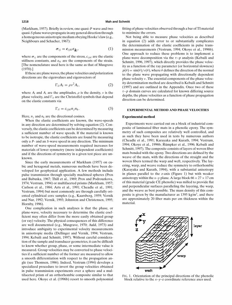
Experiments were carried out on a block of industrial com-posite of laminated fiber mats in a phenolic epoxy. The sym-metry of such composites are relatively well controlled, andas such they have been used in tests by numerous authors(Cheadle et al., 1991; Karayaka and Kurath, 1994; Vestrum,1994; Okoye et al., 1996b; Rumpker et al., 1996; Kebaili andSchmitt, 1997). The composite consists of layers of woven fibermats bonded with the epoxy. Two directions are defined by theweave of the mats, with the directions of the straight and thewoven fibers termed the warp and weft, respectively. The lay-ering, warp, and weave reduce the symmetry to orthorhombic(Karayaka and Kurath, 1994), with a substantial anisotropyin planes parallel to the z-axis (Figure 1) but with weakeranisotropy within the x–y plane. A large block 66× 27× 17 cmof this material (grade CE phenolic) was milled to provide flatand perpendicular surfaces paralleling the layering, the warp,and the weave as best possible. The mass density of this com-posite is given by the manufacturer as 1395 kg/m3, and thereare approximately 20 fiber mats per cm thickness within thematerial.

FIG. 1. Orientation of the principal directions of the phenolicblock relative to the x–y–z coordinate reference axes used.

Determination of Elastic Coefficients 1219

One P-wave and two S-wave transducers that acted asboth sources and receivers were prepared from piezoelectricceramics (Mah and Schmitt, 2001). The transducers were madeas small as possible so the transducer dimension effects couldbe ignored. The P-wave transducers were prepared from com-monly available lead zirconate sheets by cutting into 2.0-mmsquares using a computer-controlled diamond saw used in elec-tronic chip manufacturing. These transducers expand predom-inantly in the direction perpendicular to the block surface. Thenominal resonant frequency of these transducers is 1.0 MHz.The S-wave piezoelectric ceramics with a resonant frequencyof 0.65 MHz were cut into 2× 3-mm rectangles in two perpen-dicular directions to make transducers preferentially sensitiveto the different quasi-S-wave polarizations. The two cutsproduce displacements parallel to the surface of the test piece,referred to as SV and SH, which are also parallel and perpen-dicular to the source–receiver array plane, respectively. Thesedesignations of P, SV, and SHpolarization should not be takentoo literally, especially when used over complex anisotropicmedia with quasi-P and quasi-S polarizations. These desig-nations simply refer to the mode which is attempted to bepreferentially generated, given the experimental limitations.

Because of directional constraints, the SV transducers werepoor transmitters, although they were still used in reception.The P transducers better generated SV-like polarizations andwere consequently used for transmitting in both the P and SVarrays. This is expected because the P transducers act as verticalpoint sources that also generate an SV radiation pattern withsubstantial energy at oblique angles. Tests of these transducersand of the τ–p method were performed on a test sample ofisotropic, homogeneous glass (Mah and Schmitt, 2001). Thesetests suggested that uncertainties of less than 1.0% may beexpected using the τ–p technique under well-controlled con-ditions for a homogeneous material.

Phase velocities

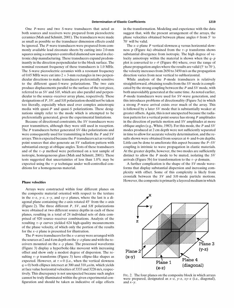
Arrays were constructed within four different planes onthe composite material oriented with respect to the texturein the x–z, y–z, x–y, and xy–z planes, where the last is a di-agonal plane containing the z-axis rotated 45◦ from the x-axis(Figure 2). The three different P, SV, and SH polarizationswere obtained at two different source depths in each of theseplanes, resulting in a total of 24 individual sets of data com-prised of 920 source–receiver combinations. Analysis of theresulting τ–p curves yielded 624 high-quality measurementsof the phase velocity, of which only the portion of the resultsfor the x–z plane is presented for illustration.

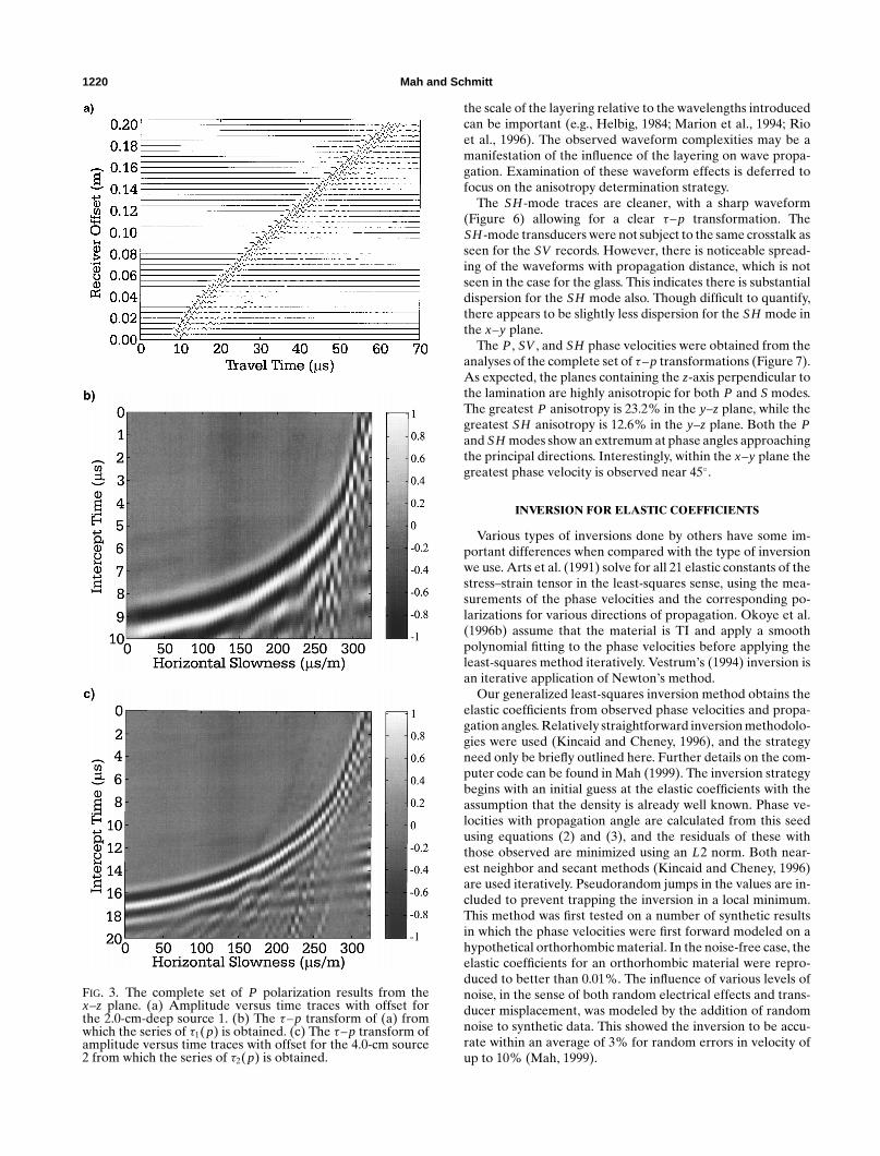
The P-wave transducers for the x–zarray were arranged withthe sources at 2 and 4 cm depth on the y–zplane and with the re-ceivers mounted on the x–y plane. The processed waveforms(Figure 3) display a hyperbolic-like moveout with increasingoffset and show only a modest degree of dispersion. The re-sulting τ–p transforms (Figure 3) have ellipse-like shapes asexpected. However, at τ = 0 (i.e., when the vertical slownessq= 0) both ellipses intersect at 300 and 310 µs/m, which yieldsat face value horizontal velocities of 3333 and 3226 m/s, respec-tively. This discrepancy is not unexpected because such anglescannot be truly illuminated within the given experimental con-figuration and should be taken as indicative of edge effects

in the transformation. Modeling and experience with the datasuggest that, with the present arrangement of the arrays, thephase velocities obtained between phase angles θ from 5◦ to70◦ will be valid.

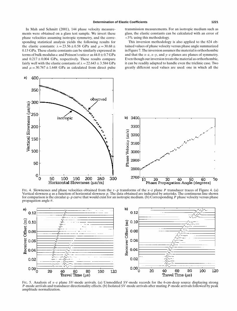
The x–z plane P vertical slowness q versus horizontal slow-ness p (Figure 4a) obtained from the τ–p transforms showssubstantial divergence from isotropic. The high degree of ve-locity anisotropy within the material is shown when the q–pplot is converted to ν–θ (Figure 4b) where, over the range ofphase propagation angles where the results are valid (5◦ to 70◦),the velocity increases from 2650 to 3450 m/s as the propagationdirection varies from near vertical to subhorizontal.

While analysis of the P-mode transducers is relativelystraightforward, obtaining results from the SVmode is compli-cated by the strong coupling between the P and SVmode, withboth unavoidably generated at the same time. As noted earlier,P-mode transducers were used for SV-wave generation, andthis introduces problems of directionality (Figure 5a) in whicha strong P-wave arrival exists over much of the array. Thisis followed by a later SV mode that is substantially weaker atgreater offsets. Again, this is not unexpected because the radia-tion pattern for a vertical point source has strong P amplitudesin the direction of particle motion and SV amplitudes at moreoblique angles (e.g., White, 1983). For this mode, the P and SVmodes produced at 2 cm depth were not sufficiently separatedin time to allow for accurate velocity determination, and the re-sults shown were obtained from sources at 4- and 6-cm depths.Little can be done to ameliorate this aspect because the P–SVcoupling is intrinsic to wave propagation in elastic materials.At the greater depths, however, the two modes are sufficientlydistinct to allow the P mode to be muted, isolating the SVarrivals (Figure 5b) for transformation to the τ–p domain.

A further complication is the shape of the SV-mode wave-forms that display substantial dispersion and increasing com-plexity with offset. Some of this complexity is likely fromcrosstalk between the SV and SH-mode particle motions.However, the composite is primarily a layered medium in which

FIG. 2. The four planes on the composite block in which arrayswere prepared, designated as x–z, y–z, xy–z (i.e., diagonal),and x–y.


FIG. 3. The complete set of P polarization results from thex–z plane. (a) Amplitude versus time traces with offset forthe 2.0-cm-deep source 1. (b) The τ–p transform of (a) fromwhich the series of τ1(p) is obtained. (c) The τ–p transform ofamplitude versus time traces with offset for the 4.0-cm source2 from which the series of τ2(p) is obtained.

the scale of the layering relative to the wavelengths introducedcan be important (e.g., Helbig, 1984; Marion et al., 1994; Rioet al., 1996). The observed waveform complexities may be amanifestation of the influence of the layering on wave propa-gation. Examination of these waveform effects is deferred tofocus on the anisotropy determination strategy.

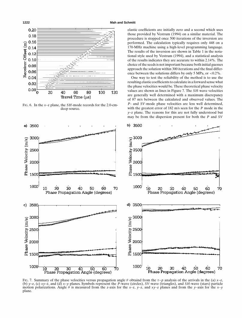
The SH-mode traces are cleaner, with a sharp waveform(Figure 6) allowing for a clear τ–p transformation. TheSH-mode transducers were not subject to the same crosstalk asseen for the SV records. However, there is noticeable spread-ing of the waveforms with propagation distance, which is notseen in the case for the glass. This indicates there is substantialdispersion for the SH mode also. Though difficult to quantify,there appears to be slightly less dispersion for the SH mode inthe x–y plane.

The P, SV, and SH phase velocities were obtained from theanalyses of the complete set of τ–p transformations (Figure 7).As expected, the planes containing the z-axis perpendicular tothe lamination are highly anisotropic for both P and Smodes.The greatest P anisotropy is 23.2% in the y–z plane, while thegreatest SH anisotropy is 12.6% in the y–z plane. Both the Pand SHmodes show an extremum at phase angles approachingthe principal directions. Interestingly, within the x–y plane thegreatest phase velocity is observed near 45◦.

INVERSION FOR ELASTIC COEFFICIENTS

Various types of inversions done by others have some im-portant differences when compared with the type of inversionwe use. Arts et al. (1991) solve for all 21 elastic constants of thestress–strain tensor in the least-squares sense, using the mea-surements of the phase velocities and the corresponding po-larizations for various directions of propagation. Okoye et al.(1996b) assume that the material is TI and apply a smoothpolynomial fitting to the phase velocities before applying theleast-squares method iteratively. Vestrum’s (1994) inversion isan iterative application of Newton’s method.

Our generalized least-squares inversion method obtains theelastic coefficients from observed phase velocities and propa-gation angles. Relatively straightforward inversion methodolo-gies were used (Kincaid and Cheney, 1996), and the strategyneed only be briefly outlined here. Further details on the com-puter code can be found in Mah (1999). The inversion strategybegins with an initial guess at the elastic coefficients with theassumption that the density is already well known. Phase ve-locities with propagation angle are calculated from this seedusing equations (2) and (3), and the residuals of these withthose observed are minimized using an L2 norm. Both near-est neighbor and secant methods (Kincaid and Cheney, 1996)are used iteratively. Pseudorandom jumps in the values are in-cluded to prevent trapping the inversion in a local minimum.This method was first tested on a number of synthetic resultsin which the phase velocities were first forward modeled on ahypothetical orthorhombic material. In the noise-free case, theelastic coefficients for an orthorhombic material were repro-duced to better than 0.01%. The influence of various levels ofnoise, in the sense of both random electrical effects and trans-ducer misplacement, was modeled by the addition of randomnoise to synthetic data. This showed the inversion to be accu-rate within an average of 3% for random errors in velocity ofup to 10% (Mah, 1999).


In Mah and Schmitt (2001), 144 phase velocity measure-ments were obtained on a glass test sample. We invert thesephase velocities assuming isotropic symmetry, and the corre-sponding statistical analysis yields the following results forthe elastic constants: λ= 23.56± 0.58 GPa and µ= 30.68±0.13 GPa. These elastic constants can be similarly expressed interms of bulk modulus κ and Poisson’s ratio σ as 44.0± 0.7 GPaand 0.217± 0.004 GPa, respectively. These results comparefairly well with the elastic constants of λ= 22.643± 3.584 GPaand µ= 30.767± 1.648 GPa as calculated from direct pulse

FIG. 4. Slownesses and phase velocities obtained from the τ–p transforms of the x–z plane P transducer traces of Figure 4. (a)Vertical slowness q as a function of horizontal slowness p. The data obtained are indicated by asterisks. The continuous line shownfor comparison is the circular q–p curve that would exist for an isotropic medium. (b) Corresponding P phase velocity versus phasepropagation angle θ .

FIG. 5. Analysis of x–z plane SV-mode arrivals. (a) Unmodified SV-mode records for the 6-cm-deep source displaying strongP-mode arrivals and transducer directionality effects. (b) Isolated SV-mode arrivals after muting P-mode arrivals followed by peakamplitude normalization.

transmission measurements. For an isotropic medium such asglass, the elastic constants can be calculated with an error of<3% using this methodology.

This inversion methodology is also applied to the 624 ob-tained values of phase velocity versus phase angle summarizedin Figure 7. The inversion assumes the material is orthorhombicand that the x–z, x–y, and y–z planes are planes of symmetry.Even though our inversion treats the material as orthorhombic,it can be readily adapted to handle even the triclinic case. Twogreatly different seed values are used: one in which all the


FIG. 6. In the x–z plane, the SH-mode records for the 2.0-cm-deep source.

FIG. 7. Summary of the phase velocities versus propagation angle θ obtaind from the τ–p analysis of the arrivals in the (a) x–z,(b) y–z, (c) xy–z, and (d) x–y planes. Symbols represent the P-wave (circles), SV-wave (triangles), and SH-wave (stars) particlemotion polarizations. Angle θ is measured from the z-axis for the x–z, y–z, and xy–z planes and from the y–axis for the x–yplane.

elastic coefficients are initially zero and a second which usesthose provided by Vestrum (1994) on a similar material. Theprocedure is stopped once 500 iterations of the inversion areperformed. The calculation typically requires only 448 on a170-MHz machine using a high-level programming language.The results of the inversion are shown in Table 1 in the nota-tional style used by Vestrum (1994), and a statistical analysisof the results indicates they are accurate to within 2.14%. Thechoice of the seeds is not important because both initial guessesapproach the solution within 300 iterations and the final differ-ence between the solutions differs by only 5 MPa, or <0.2%.

One way to test the reliability of the method is to use theresulting elastic coefficients to calculate in a forward sense whatthe phase velocities would be. These theoretical phase velocityvalues are shown as lines in Figure 7. The SH-wave velocitiesare generally well determined with a maximum discrepancyof 87 m/s between the calculated and observed values. TheP- and SV-mode phase velocities are less well determined,with the greatest error of 182 m/s seen for the P mode in they–z plane. The reasons for this are not fully understood butmay be from the dispersion present for both the P and SV


waveforms. Further, the degree of error is expected to be higherfor the SV mode becauuse of the problems already indicated.Since, even in the anisotropic medium, these two modes willbe preferentially coupled relative to the SH mode, it mightbe expected that this coupling will introduce error into the P-mode determinations.

DISCUSSION

Measurement geometry

It is useful to consider how the measurements may beoptimized—that is, the least amount of data that should beobtained. Examination of the fully expanded equation (1) inthe manner of Neighbours and Schacher (1967) reveals thatvelocities need to be measured in the three orthogonal planesof symmetry of an orthorhombic material. If these planes arenot known, then an additional diagonal plane must be inves-tigated to help localize the results. If the situation arises thatno information about the axes of symmetry of the orthorhom-bic material is known or that the material is indeed triclinic,a more general approach must be taken. At minimum, in themost general approach velocities must be measured in threeplanes oriented along an arbitrary set of axes plus two furthermutually oriented perpendicular planes running diagonally tothis set of axes. An additional third diagonal plane is recom-mended for a total of six distinct planes to most accuratelydetermine the 21 independent elastic stiffnesses.

Dispersion

Although a set of nine elastic coefficients was readily de-termined from the observed phase velocities in the inver-sion, some experimental problems remain. The most impor-tant is substantial dispersion. This dispersion is evident in allthe records of the P-, SV-, and SH-mode waveforms seen inFigures 3, 5, and 6. This dispersion is only weakly, if at all,detectable in the corresponding measurements on glass—anearly ideal, high Q, elastic medium (Mah and Schmitt, 2001)—suggesting that the dispersion may in part be a consequence ofthe structure of the material. This dispersion must have someinfluence on the accuracy of the τ–p method of phase velocitydetermination and needs to be considered in the future (seeMartinez and McMechan, 1984).

Although portions of the dispersion are possible from in-trinsic attenuation, it is also likely that part of the effect maybe a consequence of wave propagation through the layeredstructure of the composite. Although difficult to quantify, thereappears to be less dispersion in the x–y plane waveforms, sug-gesting that the observed dispersion is symptomatic of the lay-ering. Indeed, such layering-induced dispersion is not unex-pected, especially once the dimensions of the layers approachthe wavelength of the illuminating elastic wave energy (e.g.,Helbig, 1984). This may be the case in the present material as

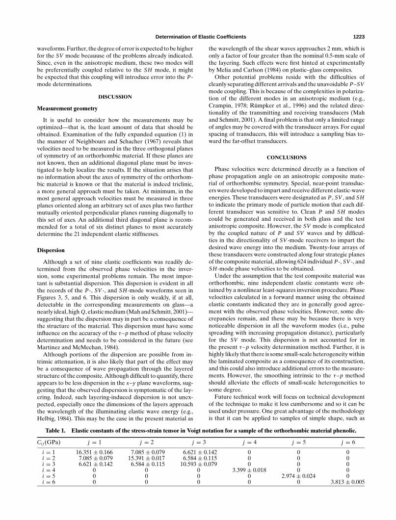
Table 1. Elastic constants of the stress-strain tensor in Voigt notation for a sample of the orthorhombic material phenolic.

Ci j (GPa) j = 1 j = 2 j = 3 j = 4 j = 5 j = 6

i = 1 16.351 ± 0.166 7.085 ± 0.079 6.621 ± 0.142 0 0 0i = 2 7.085 ± 0.079 15.391 ± 0.017 6.584 ± 0.115 0 0 0i = 3 6.621 ± 0.142 6.584 ± 0.115 10.593 ± 0.079 0 0 0i = 4 0 0 0 3.399 ± 0.018 0 0i = 5 0 0 0 0 2.974 ± 0.024 0i = 6 0 0 0 0 0 3.813 ± 0.005

the wavelength of the shear waves approaches 2 mm, which isonly a factor of four greater than the nominal 0.5-mm scale ofthe layering. Such effects were first hinted at experimentallyby Melia and Carlson (1984) on plastic–glass composites.

Other potential problems reside with the difficulties ofcleanly separating different arrivals and the unavoidable P–SVmode coupling. This is because of the complexities in polariza-tion of the different modes in an anisotropic medium (e.g.,Crampin, 1978; Rumpker et al., 1996) and the related direc-tionality of the transmitting and receiving transducers (Mahand Schmitt, 2001). A final problem is that only a limited rangeof angles may be covered with the transducer arrays. For equalspacing of transducers, this will introduce a sampling bias to-ward the far-offset transducers.

CONCLUSIONS

Phase velocities were determined directly as a function ofphase propagation angle on an anisotropic composite mate-rial of orthorhombic symmetry. Special, near-point transduc-ers were developed to impart and receive different elastic-waveenergies. These transducers were designated as P, SV, and SHto indicate the primary mode of particle motion that each dif-ferent transducer was sensitive to. Clean P and SH modescould be generated and received in both glass and the testanisotropic composite. However, the SV mode is complicatedby the coupled nature of P and SV waves and by difficul-ties in the directionality of SV-mode receivers to impart thedesired wave energy into the medium. Twenty-four arrays ofthese transducers were constructed along four strategic planesof the composite material, allowing 624 individual P-, SV-, andSH-mode phase velocities to be obtained.

Under the assumption that the test composite material wasorthorhombic, nine independent elastic constants were ob-tained by a nonlinear least-squares inversion procedure. Phasevelocities calculated in a forward manner using the obtainedelastic constants indicated they are in generally good agree-ment with the observed phase velocities. However, some dis-crepancies remain, and these may be because there is verynoticeable dispersion in all the waveform modes (i.e., pulsespreading with increasing propagation distance), particularlyfor the SV mode. This dispersion is not accounted for inthe present τ–p velocity determination method. Further, it ishighly likely that there is some small-scale heterogeneity withinthe laminated composite as a consequence of its construction,and this could also introduce additional errors to the measure-ments. However, the smoothing intrinsic to the τ–p methodshould alleviate the effects of small-scale heterogeneities tosome degree.

Future technical work will focus on technical developmentof the technique to make it less cumbersome and so it can beused under pressure. One great advantage of the methodologyis that it can be applied to samples of simple shape, such as


rectangular prisms and even cylinders. The latter will be partic-ularly useful in the context of determining anisotropy in shales,which are often assumed to be TI using core samples witha minimum of additional preparation. Of more fundamentalconcern, however, is the potential for experimental tests of thetrade-off between wave velocity anisotropy, dispersion, andscale in layered anisotropic media; this has implications be-yond laboratory determination of elastic properties. The τ–pmethod will aid in such fundamental studies of layered media.

ACKNOWLEDGMENTS

This work was supported by NSERC and the Petroleum Re-search Fund administered by the American Chemical Society.Technical assistance and sample preparation was greatly as-sisted by R. Hunt, L. Tober, and R. Tomski. The work of Kebailiand Molz prepared the way for the present experiment. Theassistance of the Alberta Microelectronics Centre in cuttingthe ceramic transducers is greatly appreciated. The use of thecomputer equipment and software of the Downhole SeismicImaging Consortium during the preparation of this paper isappreciated.

REFERENCES

Arts, R. J., Rasolofosaon, P. N. J., and Zinszner, B. E., 1991, Completeinversion of the anisotropic elastic tensor in rocks: Experiment ver-sus theory: 61st Ann. Internat. Mtg., Soc. Expl. Geophys., ExpandedAbstracts, 1538–1541.

Auld, B. A., 1973, Acoustic fields and waves in solids: John Wiley &Sons, Inc.

Carlson, R. L., Schaftenaar, C. H., and Moore, R. P., 1984, Causes ofcompressional-wave anisotropy in carbonate-bearing, deep-sea sed-iments: Geophysics, 49, 525–532.

Cheadle, S. P., Brown, R. J., and Lawton, D. C., 1991, Orthorhom-bic anisotropy: A physical seismic modeling study: Geophysics, 56,1603–1613.

Claerbout, J. F., 1985, Imaging the earth’s interior: Blackwell ScientificPublications, Inc.

Crampin, S., 1978, Seismic-wave propagation through a cracked solid:Polarization as a possible dilatancy diagnostic: Geophys. J. Roy. Astr.Soc., 53, 467–496.

Dellinger, J., and Vernik, L., 1994, Do traveltimes in pulse-transmissionexperiments yield anisotropic group or phase velocities?: Geo-physics, 59, 1774–1779.

Helbig, K., 1984, Anisotropy and dispersion in periodically layeredmedia: Geophysics, 49, 364–373.

Hornby, B., 1996, Experimental determination of anisotropic proper-ties of shales, in Fjaer, E., Holt, R. M., and Rathore, J. S., Eds., Seismicanisotropy: Soc. Expl. Geophys., 238–296.

Johnston, J. E., and Christensen, N. I., 1995, Seismic anisotropy ofshales: J. Geophys. Res., 100, 5991–6003.

Kaarsberg, E. A., 1959, Introductory studies of natural and artificialargillaceous aggregates by sound-propagation and x-ray diffractionmethods: J. Geol., 67, 447–472.

Karayaka, M., and Kurath, P., 1994, Deformation and failure behaviourof woven composite laminates: J. Eng. Mat. and Technol., 116, 222–232.

Kebaili, A., and Schmitt, D. R., 1996, Velocity anisotropy observed inwellbore seismic arrivals: Combined effects of intrinsic propertiesand layering: Geophysics, 61, 12–20.

——— 1997, Ultrasonic anisotropic phase velocity determination withthe Radon transformation: J. Acoust. Soc. Am., 101, 3278–3286.

Kincaid, D., and Cheney, W., 1996, Numerical analysis: Brooks/ColePubl. Co.

Mah, M., 1999, Experimental determination of the elastic coefficientsof anisotropic materials with the slant-stack method: MS thesis, Univ.of Alberta.

Mah, M., and Schmitt, D. R., 2001, Near point-source longitudinaland transverse mode ultrasonic arrays for material characterization:IEEE Trans. Ultrason., Ferroelect., Freq. Contr., 48, 691–698.

Marion, D., Mukerji, T., and Mavko, G., 1994, Scale effects on veloc-ity dispersion: From ray to effective medium theories in stratifiedmedia: Geophysics, 59, 1613–1619.

Markham, M. F., 1957, Measurement of elastic constants by the ultra-sonic pulse method: Brit. J. Appl. Phys., 6, 56–63.

Martinez, R. D., and McMechen, G. A., 1984, Analysis of absorptionand dispersion effects in tau-p synthetic seismograms: 54th Ann.Internat. Mtg., Soc. Expl. Geophys., Expanded Abstracts, sessionS24.2.

Melia, P. J., and Carlson, R. L., 1984, An experimental test of P-waveanisotropy in stratified media: Geophysics, 49, 374–378.

Musgrave, M. J. P., 1970, Crystal acoustics: Holden-Day.Neighbours, J. R., and Schacher, G. E., 1967, Determination of elastic

constants from sound–velocity measurements in crystals of generalsymmetry: J. Appl. Phys., 38, 5366–5375.

Okoye, P. N., Uren, N. F., MacDonald, J. A., and Ebrom, D. A., 1996a,Variation of spatial resolution with orientation of symmetry axis inanisotropic media, in Fjaer, E., Holt, R. M., and Rathore, J. S., Eds.,Seismic anisotropy: Soc. Expl. Geophys., 76–99.

Okoye, P. N., Zhao, P., and Uren, N. F., 1996b, Inversion technique forrecovering the elastic constants of transversely isotropic materials:Geophysics, 61, 1247–1257.

Pros, Z., and Babuska, V., 1967, A method for investigating the elasticanisotropy on spherical rock samples: Z. Geophys., 33, 289–291.

Pros, Z. and Podrouzkova, Z., 1974, Apparatus for investigating theelastic anisotropy of spherical samples at high pressure: Veroof. Zen-tral Inst. Phys. Erde, 22, 42–47.

Rio, P., Mukerji, T., Mavko, G., and Marion, D., 1996, Velocity disper-sion and upscaling in a laboratory-simulated VSP: Geophysics, 61,584–593.

Rumpker, G., Brown, R. J., and Thomson, C. J., 1996, Shear wave prop-agation in orthorhombic phenolic: A comparison of numerical andphysical modeling: J. Geophys. Res., 101, 27 765–27 777.

Thill, R. E., Willard, R. J., and Bur, T. R., 1969, Correlation of lon-gitudinal velocity variation with rock fabric: J. Geophys. Res., 74,4897–4909.

Thomsen, L., 1986, Weak elastic anisotropy: Geophysics, 51, 1954–1966.

Vernik, L., 1993, Microcrack-induced versus intrinsic elastic anisotropyin mature HC-source shales: Geophysics, 58, 1703–1706.

Vernik, L., and Nur, A., 1992, Ultrasonic velocity and anisotropy ofhydrocarbon source rocks: Geophysics, 57, 727–735.

Vestrum, R. W., 1994, Group and phase-velocity inversions for thegeneral anisotropic stiffness tensor: MS thesis, Univ. of Calgary.

White, J. E., 1983, Underground sound: Elsevier Science Publ. Co. Inc.

APPENDIX

PLANE-WAVE DECOMPOSITION

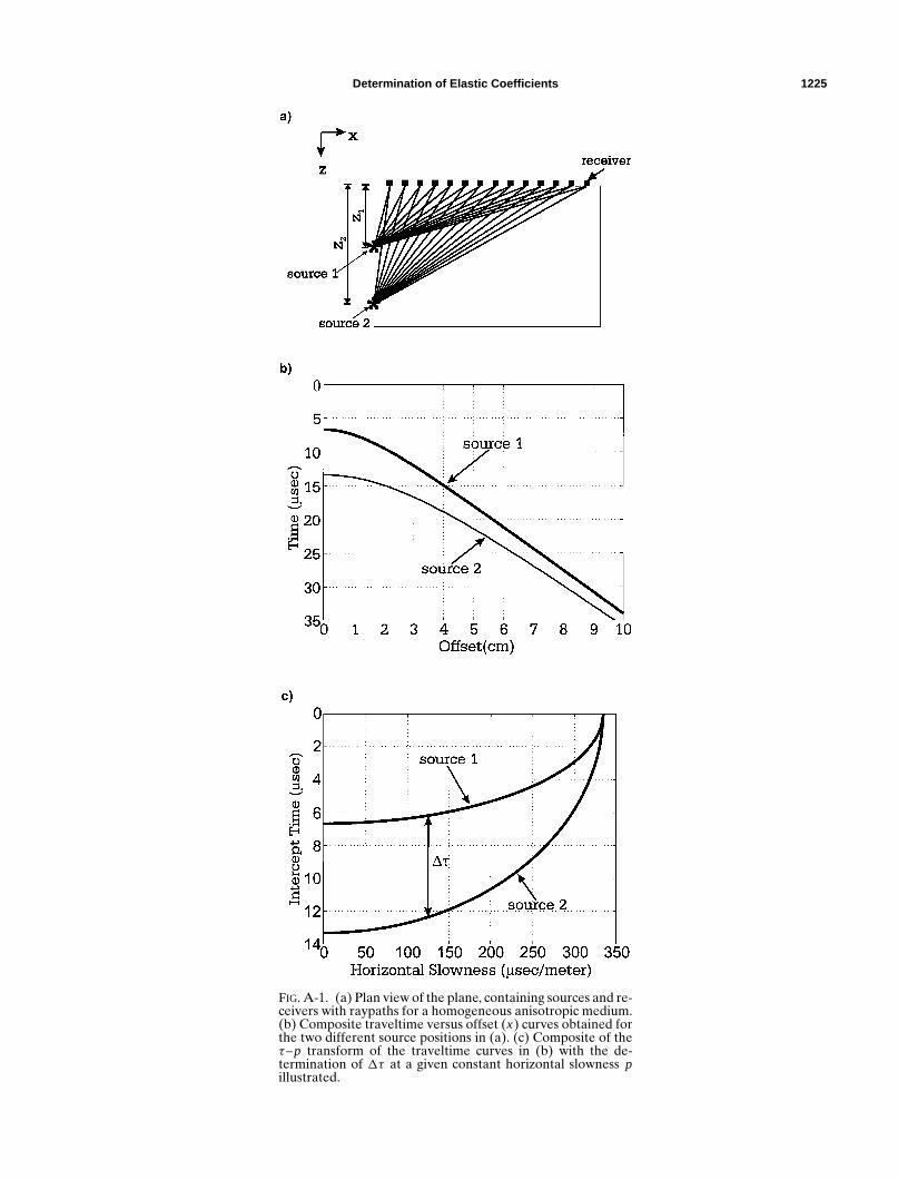
In the technique, the pulsed elastic wave energy producedfrom a minimum of two source transducers is detected by acoplanar array of receiving transducers mounted on the adja-cent side of the test piece (Figure A-1a). The sets of arrivaltimes from each of the two transducers yield hyperbolic-likeoffset versus traveltime curves in the x–t domain (Figure 1b),which transform to ellipse-like curves in the τ–p domain (Fig-ure 1c). If the block of material is homogeneous, then at con-stant horizontal slowness p the vertical slowness q is (Kebailiand Schmitt, 1997)

q(p) = τ2(p)− τ1(p)z2 − z1

, (A-1)

where τ1 and τ2 are the intercept times at constant p corre-sponding from the τ–p curves for the sources at offsets z1

and z2, respectively (Figure 1c). It is worth noting that q in ananisotropic material depends on the horizontal slowness p andis hence also implicitly dependent on the propagation angle θwithin the plane. The phase velocity ν is then

ν(θ) = (q2(θ)+ p2(θ))−1/2 (A-2)

at the phase propagation angle

θ = arctan(

p

q

). (A-3)


FIG. A-1. (a) Plan view of the plane, containing sources and re-ceivers with raypaths for a homogeneous anisotropic medium.(b) Composite traveltime versus offset (x) curves obtained forthe two different source positions in (a). (c) Composite of theτ–p transform of the traveltime curves in (b) with the de-termination of 1τ at a given constant horizontal slowness pillustrated.

experimental determination of the elastic coefficients of ...dschmitt/papers/experimental... ·...

Documents