Expectation of Random Variables

Saravanan Vijayakumaransarva@ee.iitb.ac.in

Department of Electrical EngineeringIndian Institute of Technology Bombay

February 13, 2015

1 / 19

Expectation of Discrete Random Variables

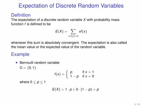
DefinitionThe expectation of a discrete random variable X with probability massfunction f is defined to be

E(X ) =∑

x :f (x)>0

xf (x)

whenever this sum is absolutely convergent. The expectation is also calledthe mean value or the expected value of the random variable.

Example

• Bernoulli random variableΩ = 0, 1

f (x) =

p if x = 11− p if x = 0

where 0 ≤ p ≤ 1

E(X ) = 1 · p + 0 · (1− p) = p

2 / 19

More Examples

• The probability mass function of a binomial random variable X withparameters n and p is

P[X = k ] =

(nk

)pk (1− p)n−k if 0 ≤ k ≤ n

Its expected value is given by

E(X ) =n∑

k=0

kP[X = k ] =n∑

k=0

k

(nk

)pk (1− p)n−k = np

• The probability mass function of a Poisson random variable withparameter λ is given by

P[X = k ] =λk

k !e−λ k = 0, 1, 2, . . .

Its expected value is given by

E(X ) =∞∑

k=0

kP[X = k ] =∞∑

k=0

kλk

k !e−λ = λ

3 / 19

Why do we need absolute convergence?

• A discrete random variable can take a countable number of values

• The definition of expectation involves a weighted sum of these values

• The order of the terms in the infinite sum is not specified in the definition

• The order of the terms can affect the value of the infinite sum

• Consider the following series

1− 12

+13− 1

4+

15− 1

6+

17− 1

8+ · · ·

Its sums to a value less than 56

• Consider a rearrangement of the above series where two positive termsare followed by one negative term

1 +13− 1

2+

15

+17− 1

4+

19

+1

11− 1

6+ · · ·

Since1

4k − 3+

14k − 1

− 12k

> 0

the rearranged series sums to a value greater than 56

4 / 19

Why do we need absolute convergence?

• A series∑

ai is said to converge absolutely if the series∑|ai |

converges

• Theorem: If∑

ai is a series which converges absolutely, then everyrearrangement of

∑ai converges, and they all converge to the same

sum

• The previously considered series converges but does not convergeabsolutely

1− 12

+13− 1

4+

15− 1

6+

17− 1

8+ · · ·

• Considering only absolutely convergent sums makes the expectationindependent of the order of summation

5 / 19

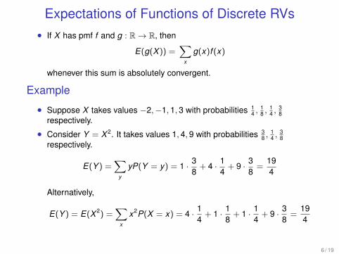
Expectations of Functions of Discrete RVs• If X has pmf f and g : R→ R, then

E(g(X )) =∑

x

g(x)f (x)

whenever this sum is absolutely convergent.

Example

• Suppose X takes values −2,−1, 1, 3 with probabilities 14 ,

18 ,

14 ,

38

respectively.

• Consider Y = X 2. It takes values 1, 4, 9 with probabilities 38 ,

14 ,

38

respectively.

E(Y ) =∑

y

yP(Y = y) = 1 · 38

+ 4 · 14

+ 9 · 38

=194

Alternatively,

E(Y ) = E(X 2) =∑

x

x2P(X = x) = 4 · 14

+ 1 · 18

+ 1 · 14

+ 9 · 38

=194

6 / 19

Expectation of Continuous Random VariablesDefinitionThe expectation of a continuous random variable with density function f isgiven by

E(X ) =

∫ ∞−∞

xf (x) dx

whenever this integral is finite.

Example (Uniform Random Variable)

f (x) =

1b−a for a ≤ x ≤ b0 otherwise

x

f (x)

a b

1b−a

E(X ) = a+b2

7 / 19

Conditional ExpectationDefinitionFor discrete random variables, the conditional expectation of Y given X = xis defined as

E(Y |X = x) =∑

y

yfY |X (y |x)

For continuous random variables, the conditional expectation of Y given X isgiven by

E(Y |X = x) =

∫ ∞−∞

yfY |X (y |x) dy

The conditional expectation is a function of the conditioning random variablei.e. ψ(X ) = E(Y |X )

ExampleFor the following joint probability mass function, calculate E(Y ) and E(Y |X ).

Y ↓,X → x1 x2 x3

y112 0 0

y2 0 18

18

y3 0 18

18

8 / 19

Law of Iterated Expectation

TheoremThe conditional expectation E(Y |X ) satisfies

E [E(Y |X )] = E(Y )

ExampleA group of hens lay N eggs where N has a Poisson distribution withparameter λ. Each egg results in a healthy chick with probability pindependently of the other eggs. Let K be the number of chicks. Find E(K ).

9 / 19

Some Properties of Expectation

• If a, b ∈ R, then E(aX + bY ) = aE(X ) + bE(Y )

• If X and Y are independent, E(XY ) = E(X )E(Y )

• X and Y are said to be uncorrelated if E(XY ) = E(X )E(Y )

• Independent random variables are uncorrelated but uncorrelatedrandom variables need not be independent

ExampleY and Z are independent random variables such that Z is equally likely to be1 or −1 and Y is equally likely to be 1 or 2.Let X = YZ . Then X and Y are uncorrelated but not independent.

10 / 19

Expectation via the Distribution FunctionFor a discrete random variable X taking values in 0, 1, 2, . . ., the expectedvalue is given by

E [X ] =∞∑i=1

P(X ≥ i)

Proof

∞∑i=1

P(X ≥ i) =∞∑i=1

∞∑j=i

P(X = j) =∞∑j=1

j∑i=1

P(X = j) =∞∑j=1

jP(X = j) = E [X ]

ExampleLet X1, . . . ,Xm be m independent discrete random variables taking onlynon-negative integer values. Let all of them have the same probability massfunction P(X = n) = pn for n ≥ 0. What is the expected value of theminimum of X1, . . . ,Xm?

11 / 19

Expectation via the Distribution FunctionFor a continuous random variable X taking only non-negative values, theexpected value is given by

E [X ] =

∫ ∞0

P(X ≥ x) dx

Proof

∫ ∞0

P(X ≥ x) dx =

∫ ∞0

∫ ∞x

fX (t) dt dx =

∫ ∞0

∫ t

0fX (t) dx dt

=

∫ ∞0

tfX (t) dt = E [X ]

12 / 19

Variance

• Quantifies the spread of a random variable

• Let the expectation of X be m1 = E(X )

• The variance of X is given by σ2 = E [(X −m1)2]

• The positive square root of the variance is called the standard deviation

• Examples

• Variance of a binomial random variable X with parameters n and pis

var(X ) =n∑

k=0

(k − np)2P[X = k ] =n∑

k=0

k2

(nk

)pk (1− p)n−k − n2p2

= np(1− p)

• Variance of a uniform random variable X on [a, b] is

var(X ) =

∫ ∞−∞

[x − a + b

2

]2

fU(x) dx =(b − a)2

12

13 / 19

Properties of Variance

• var(X ) ≥ 0

• var(X ) = E(X 2)− [E(X )]2

• For a, b ∈ R, var(aX + b) = a2 var(X )

• var(X + Y ) = var(X ) + var(Y ) if and only if X and Y are uncorrelated

14 / 19

Probabilistic Inequalities

Markov’s InequalityIf X is a non-negative random variable and a > 0, then

P(X ≥ a) ≤ E(X )

a.

ProofWe first claim that if X ≥ Y , then E(X ) ≥ E(Y ).Let Y be a random variable such that

Y =

a if X ≥ a,0 if X < a.

Then X ≥ Y and E(X ) ≥ E(Y ) = aP(X ≥ a) =⇒ P(X ≥ a) ≤ E(X)a .

Exercise• Prove that if E(X 2) = 0 then P(X = 0) = 1.

16 / 19

Chebyshev’s InequalityLet X be a random variable and a > 0. Then P (|X − E(X )| ≥ a) ≤ var(X)

a2 .

ProofLet Y = (X − E(X ))2.

P (|X − E(X )| ≥ a) = P(Y ≥ a2) ≤ E(Y )

a2 =var(X )

a2 .

Setting a = kσ where k > 0 and σ =√

var(X ), we get

P (|X − E(X )| ≥ kσ) ≤ 1k2 .

Exercises• Suppose we have a coin with an unknown probability p of showing

heads. We want to estimate p to within an accuracy of ε > 0. How canwe do it?

• Prove that P(X = c) = 1 ⇐⇒ var(X ) = 0.

17 / 19

Cauchy-Schwarz InequalityFor random variables X and Y , we have

|E(XY )| ≤√

E(X 2)√

E(Y 2)

Equality holds if and only if P(X = cY ) = 1 for some constant c.

ProofFor any real k , we have E [(kX + Y )2] ≥ 0. This implies

k2E(X 2) + 2kE(XY ) + E(Y 2) ≥ 0

for all k . The above quadratic must have a non-positive discriminant.

[2E(XY )]2 − 4E(X 2)E(Y 2) ≤ 0.

18 / 19

Questions?

19 / 19