Exotic Preferences for Macroeconomists∗

David K. Backus,† Bryan R. Routledge,‡ and Stanley E. Zin§

September 13, 2004

Abstract

We provide a user’s guide to “exotic” preferences: nonlinear time aggregators, departuresfrom expected utility, preferences over time with known and unknown probabilities, risk-sensitive and robust control, “hyperbolic” discounting, and preferences over sets (“tempta-tions”). We apply each to a number of classic problems in macroeconomics and finance,including consumption and saving, portfolio choice, asset pricing, and Pareto optimal allo-cations.

JEL Classification Codes: D81, D91, E1, G12.

Keywords: time preference; risk; uncertainty; ambiguity; robust control; temptation;dynamic consistency; hyperbolic discounting; precautionary saving; equity premium;risk sharing.

∗Prepared for the 2004 NBER Macroeconomics Annual. The paper is virtually the same as NBER

Working Paper 10597. The formatting is more compact and a number of minor typos have been corrected.

We are unusually grateful to the many people who made suggestions and answered questions while we

worked through this enormous body of work. Deserving special mention are Mark Gertler, Lars Hansen,

Tom Sargent, Rob Shimer, Tony Smith, Ivan Werning, Noah Williams, and especially Martin Schneider. We

also thank Pierre Collin-Dufresne, Kfir Eliaz, Larry Epstein, Anjela Kniazeva, Per Krusell, David Laibson,

John Leahy, Tom Tallarini, Stijn Van Nieuwerburgh, and seminar participants at CMU and NYU.†Stern School of Business, New York University, and NBER; dbackus@stern.nyu.edu.‡Tepper School of Business, Carnegie Mellon University; routledge@cmu.edu.§Tepper School of Business, Carnegie Mellon University, and NBER; zin@cmu.edu.

1 Introduction

Applied economists (including ourselves) are generally content to study theoretical agentswhose preferences are additive over time and across states of nature. One version goeslike this: Time is discrete, with dates t = 0, 1, 2, . . .. At each t > 0, an event zt is drawnfrom a finite set Z, following an initial event z0. The t-period history of events is denotedby zt = (z0, z1, . . . , zt) and the set of possible t-histories by Zt. The evolution of eventsand histories is conveniently illustrated by an event tree, as in Figure 1, with each branchrepresenting an event and each node a history or state. Environments like this, involvingtime and uncertainty, are the starting point for most of modern macroeconomics and finance.A typical agent in such a setting has preferences over payoffs c(zt) for each possible history.A general set of preferences might be represented by a utility function U({c(zt)}). Morecommon, however, is to impose the additive expected utility structure

U({c(zt)}) =∞∑

t=0

βt∑

zt∈Zt

p(zt)u[c(zt)] = E0

∞∑

t=0

βtu(ct), (1)

where 0 < β < 1, p(zt) is the probability of history zt, and u is a period/state utilityfunction. These preferences are remarkably parsimonious: behavior over time and acrossstates depends solely on the discount factor β, the probabilities p, and the function u.

Although (1) remains the norm throughout economics, there has been extraordinarytheoretical progress over the last fifty years (and particularly the last twenty five) in devel-oping alternatives. Some of these alternatives were developed to account for the anomalouspredictions of expected utility in experimental work. Others arose from advances in thepure theory of intertemporal choice. Whatever their origin, they offer greater flexibilityalong several dimensions, often with only a modest increase in analytical difficulty.

What follows is a user’s guide, intended to serve as an introduction and instructionmanual for economists studying problems in which the structure of preferences may playan important role. Our goal is to describe exotic preferences to mainstream economists:preferences over time, preferences across states or histories, and (especially) combinationsof the two. We take an overtly practical approach, downplaying or ignoring altogether themany technical issues that arise in specifying preferences in dynamic stochastic settings,including their axiomatic foundations. (References are provided in Appendix A for thosewho are interested.) We generally assume without comment that preferences can be rep-resented by increasing, (weakly) concave functions, with enough smoothness and boundaryconditions to generate interior solutions to optimizations. We focus instead on applications,using tractable functional forms to revisit some classic problems: consumption and saving,portfolio choice, asset pricing, and Pareto optimal allocations. In most cases, we use utilityfunctions that are homogeneous of degree one (hence invariant to scale) with constant elas-ticities (think power utility). These functions are the workhorses of macroeconomics andfinance, so little is lost by restricting ourselves in this way.

You might well ask: Why bother? Indeed, we will not be surprised if most economistscontinue to use (1) most of the time. Exotic preferences, however, have a number of potentialadvantages that we believe will lead to much wider application than we’ve seen to date.One is more flexible functional forms for approximating features of data — the equity

premium, for example. Another is the ability to ask questions that have no counterpart inthe additive model. How should we make decisions if we don’t know the probability modelthat generates the data? Can preferences be dynamically inconsistent? If they are, howdo we make decisions? What is the appropriate welfare criterion? Can we think of somechoices as tempting us away from better ones? Each of these advantages raises furtherquestions: Are exotic preferences observationally equivalent to additive preferences? If not,how do we identify their parameters? Are they an excuse for free parameters? Do we evencare whether behavior is derived from preferences?

These questions run through a series of non-additive preference models. In Section 2, wediscuss time preference in a deterministic setting, comparing Koopmans’ time aggregator tothe traditional time-additive structure. In Section 3, we describe alternatives to expectedutility in a static setting, using a certainty-equivalent function to summarize preferencetoward risk. We argue that the Chew-Dekel class extends expected utility in useful directionswithout sacrificing analytical and empirical convenience. In Section 4, we put time andrisk preference together in a Kreps-Porteus aggregator, which leads to a useful separationbetween time and risk preference. Dynamic extensions of Chew-Dekel preferences followthe well-worn path of Epstein and Zin. In Section 5, we consider risk-sensitive and robustcontrol, whose application to economics is associated with the work of Hansen and Sargent.Section 6 is devoted to ambiguity, in which agents face uncertainty over probabilities aswell as states. We describe Gilboa and Schmeidler’s “max-min” utility for static settingsand Epstein and Schneider’s recursive extension to dynamic settings. In Section 7, we turnto “hyperbolic discounting” and provide an interpretation based on Gul and Pesendorfer’s“temptation” preferences. The final section is devoted to a broader discussion of the roleand value of exotic preferences in economics.

A word on notation and terminology: We typically denote parameters by Greek lettersand functions and variables by Latin letters. We denote derivatives with subscripts; thus V2

refers to the derivative of V with respect to its second argument. In a stationary dynamicprogramming problem, J is a value function and a prime (′) distinguishes a future valuefrom a current value. The abbreviation “iid” means independent and identically distributedand NID(x, y) means normally and independently distributed with mean x and variance y.

2 Time

Time preference is a natural starting point for macroeconomists, since so much of oursubject is concerned with dynamics. Suppose there is no risk and (for this paragraphonly) ct is one-dimensional. Preferences might then be characterized by a general utilityfunction U({ct}). A common measure of time preference in this setting is the marginal rateof substitution between consumption at two consecutive dates (ct and ct+1, say) along aconstant consumption path (ct = c for all t). If the marginal rate of substitution is

MRSt,t+1 =∂U/∂ct+1

∂U/∂ct,

then time preference is captured by the discount factor

β(c) ≡ MRSt,t+1(c).

2

(Picture the slope, −1/β, of an indifference curve along the “45-degree line.”) If β(c) is lessthan one, the agent is said to be impatient: she requires more than one unit of consumptionat t + 1 to induce her to give up one unit at t. For the traditional time-additive utilityfunction,

U({ct}) =∞∑

t=0

βtu(ct), (2)

β(c) = β < 1 regardless of the value of c, so impatience is built in and constant. The restof this section is concerned with preferences in which the discount factor can vary with thelevel of consumption.

Koopmans’ time aggregator

Koopmans (1960) derives a class of stationary recursive preferences by imposing conditionson a general utility function U for a multi-dimensional consumption vector c. Our approachand terminology follow Johnsen and Donaldson (1985). Preferences at all dates come fromthe same “date-zero” utility function U . As a result, they are dynamically consistent byconstruction: preferences over consumption streams starting at any future date t are con-sistent with U . Following Koopmans, let tc ≡ (ct, ct+1, . . .) be an infinite consumptionsequence starting at t. Then we might write utility from date t = 0 on as

U(0c) = U(c0, 1c).

Koopmans’ first condition is history-independence: preferences over sequences tc do notdepend on consumption at dates prior to t. Without this condition, an agent makingsequential decisions would need to keep track of the history of consumption choices to beable to make future choices consistent with U . The marginal rate of substitution betweenconsumption at two arbitrary dates could depend, in general, on consumption at all datespast, present, and future. History-independence rules out dependence on the past. Withit, the utility function can be expressed in the form

U(0c) = V [c0, U1(1c)]

for some time aggregator V . As a result, choices over 1c do not depend on c0. (Note,for example, that marginal rates of substitution between elements of 1c do not depend onc0.) Koopmans’ second condition is future independence: preferences over ct do not dependon t+1c. (In Koopmans’ terminology, the first and second conditions together imply thatpreferences over the present (ct) and future (t+1c) are independent .) This is trivially true ifct is a scalar, but a restriction on preferences otherwise. The two conditions together implythat utility can be written

U(0c) = V [u(c0), U1(1c)]

for some functions V and u, which defines u as a composite commodity for consumption ata specific date. Koopmans’ third condition is that preferences are stationary (the same atall dates). The three conditions together imply that utility can be written in the stationaryrecursive form,

U(tc) = V [u(ct), U(t+1c)] (3)

3

for all dates t. This is a generalization of the traditional utility function (2), where (evi-dently) V (u, U) = u+βU or the equivalent. As in traditional utility theory, preferences areunchanged when we apply a monotonic transformation to U : if U = f(U) for f increasing,then we replace the aggregator V with V (u, U) = f(V [u, f−1(U)]).

In the Koopmans class of preferences represented by (3), time preference is a propertyof the time aggregator V . Consider our measure of time preference for the compositecommodity u. If Ut and ut represent U(tc) and u(ct), respectively, then

Ut = V (ut, Ut+1) = V [ut, V (ut+1, Ut+2)].

The marginal rate of substitution between ut and ut+1 is therefore

MRSt,t+1 =V2(ut, Ut+1)V1(ut+1, Ut+2)

V1(ut, Ut+1).

A constant consumption path with period utility u is defined by U = V (u, U), implyingU = g(u) = V [u, g(u)] for some function g. (Koopmans calls g the correspondence function.)The discount factor is therefore β(u) = V2[u, g(u)]. You might verify for yourself that V2 isinvariant to increasing transformations of U .

In modern applications, we generally work in reverse order: we specify a period utilityfunction u and a time aggregator V and use them to characterize the overall utility functionU . Any U constructed this way defines preferences that are dynamically consistent, historyindependent, future independent, and stationary. In contrast to time-additive preferences(2), discounting depends on the level of utility u. To get a sense of how this works, considerthe behavior of V2. If preferences are increasing in consumption, u must be increasing inc and V must be increasing in both arguments. If we consider sequences with constantconsumption, U must be increasing in u, so that

g1(u) = V1[u, g(u)] + V2[u, g(u)]g1(u) =V1[u, g(u)]

1 − V2[u, g(u)]> 0.

Since V1 > 0, 0 < V2[u, g(u)] < 1: the discount factor is between zero and one and depends(in general) on u. Many economists impose an additional condition of increasing marginalimpatience: V2[u, g(u)] is decreasing in u, or

V21[u, g(u)] + V22[u, g(u)]g1(u) = V21[u, g(u)] + V22[u, g(u)]V1[u, g(u)]

1 − V2[u, g(u)]< 0.

In applications, this condition is typically used to generate stability of steady states.

Two variants of Koopmans’ structure have been widely used by macroeconomists. Onewas proposed by Uzawa (1968), who suggested a continuous-time version of

V (u, U) = u + β(u)U.

(In his model, β(u) = exp[−δ(u)].) Since V21 = 0, increasing marginal impatience issimply β1(u) < 0 (equivalently, δ1(u) > 0). Another is used by Epstein and Hynes (1983),Lucas and Stokey (1984), and Shi (1994), who generalize Koopmans by omitting the futureindependence condition. The resulting aggregator is V (c, U), rather than V (u, U), which

4

allows choice over c to depend on U . If c is a scalar, this is equivalent to (3) (set u(c) = c),but otherwise need not be. An example is

V (c, U) = u(c) + β(c)U,

where there is no particular relationship between the functions u and β.

Examples

Example 1 (growth and fiscal policy). In the traditional growth model, Koopmans prefer-ences can change both the steady state and the short-run dynamics. Suppose the periodutility function is u(c) and the time aggregator is V (u, U ′) = u + β(u)U ′, with u increasingand concave and β1(u) < 0. Gross output y is produced with capital k using an increasingconcave technology f . The resource constraint is y = f(k) = c + k′ + g, where c is con-sumption, k′ is tomorrow’s capital stock, and g is government purchases (constant). TheBellman equation is

J(k) = maxk′

u[f(k) − k′ − g] + β(u[f(k) − k′ − g])J(k′).

The first-order and envelope conditions are

u1(c){1 + β1[u(c)]J(k′)} = β[u(c)]J1(k′)

J1(k) = u1(c)f1(k){1 + β1[u(c)]J(k′)},

which together imply J1(k) = β[u(c)]J1(k′)f1(k). In a steady state, 1 = β(u[f(k) − k −

g])f1(k).

One clear difference from the traditional model is the role of preferences in determiningthe steady state. With constant β, the steady state capital stock solves βf1(k) = 1; u isirrelevant. With recursive preferences, the steady state solves β(u[f(k) − k − g])f1(k) = 1,which depends on u through its impact on β. Consider the impact of an increase in g. Withtraditional preferences, the steady state capital stock doesn’t change, so any increase in gis balanced by an equal decrease in c. With recursive preferences and increasing marginalimpatience, an increase in g reduces current utility and therefore raises the discount factor.The initial drop in c is therefore larger than in the traditional case. In the resulting steadystate, the increase in g leads to an increase in k and a decline in c that is smaller than theincrease in g. The magnitude of the decline depends on β1, the sensitivity of the discountfactor to current utility. [Adapted from Dolmas and Wynne (1998).]

Example 2 (optimal allocations). Time preference affects the optimal allocation of consump-tion among agents over time. Consider an economy with a constant aggregate endowment yof a single good, to be divided between two agents with Koopmans preferences, representedhere by the aggregators V (the first agent) and W (the second). A Pareto optimal allocationis summarized by the Bellman equation

J(w) = maxc,w′

V [y − c, J(w′)]

subject toW (c, w′) ≥ w.

5

Note that both consumption c and promised utility w pertain to the second agent. If λ isthe Lagrange multiplier on the constraint, the first-order and envelope conditions are

V1[y − c, J(w′)] = λW1(c, w′)

V2[y − c, J(w′)]J1(w′) + λW2(c, w

′) = 0

J1(w) = −λ.

If agents’ preferences are additive with the same discount factor β, then the second andthird equations imply J1(w

′)/J1(w) = W2(c, w′)/V2[y − c, J(w′)] = β/β = 1: an optimal

allocation places the same weight λ = −J1(w) on the second agent’s utility at all dates andpromised utility w is constant. If preferences are additive and β2 > β1 (the second agent ismore patient), then J1(w

′)/J1(w) = β2/β1 > 1: an optimal allocation increases the weightover time on the second, more patient agent and raises her promised utility (w′ > w). In themore general Koopmans setting, the dynamics depend on the time aggregators V and W .The allocation converges to a steady state if both aggregators exhibit increasing marginalimpatience and future utility is a normal good. [Adapted from Lucas and Stokey (1984).]

Example 3 (long-run properties of a small open economy). Small open economies withperfect capital mobility raise difficulties with the existence of a steady state that can beresolved by endogenizing the discount factor. We represent preferences over sequences ofconsumption c and leisure 1 − n with a period utility function u(c, 1 − n) and a timeaggregator V (c, 1 − n, U) = u(c, 1 − n) + β(c, 1 − n)U . Let output be produced with laborusing the linear technology y = θn, where θ is a productivity parameter. The economy’sresource constraint is y = c + x, where x is net exports. The agent can borrow and lend ininternational capital markets at gross interest rate r, giving rise to the budget constrainta′ = r(a + x) = r(a + θn − c). The Bellman equation is

J(a) = maxc,n

u(c, 1 − n) + β(c, 1 − n)J [r(a + θn − c)].

The first-order and envelope conditions are:

u1 + β1J(a′) = βJ1(a′)

u2 + β2J(a′) = βJ1(a′)θ

J1(a) = βJ1(a′)r.

The last equation tells us that in a steady state, β(c, 1−n)r = 1. With constant discounting,there is no steady state, but with more general discounting schemes the form of discountingdetermines the steady state and its response to changes in the environment. Here thelong-run impact of a change in (say) θ (the “wage”) depends on the form of β. Supposeβ is a function of n only. Then the steady state condition β(1 − n)r = 1 determines nindependently of θ! More generally, the long-run impact on n of a change in θ depends onthe form of the discount function β(c, 1 − n). [Adapted from Epstein and Hynes (1983),Mendoza (1991), Obstfeld (1981), Schmitt-Grohe and Uribe (2002), and Shi (1994).]

Example 4 (dynamically inconsistent preferences). Suppose preferences “from date t on”are given by:

Ut(tc) = u(ct) + δβu(ct+1) + δβ2u(ct+2) + δβ3u(ct+3) + · · · ,

6

with 0 < δ ≤ 1. When δ = 1 this reduces to the time-additive utility function (2).Otherwise, we discount utility in periods t + 1, t + 2, t + 3, . . . by δβ, δβ2, δβ3, . . .. A littleeffort should convince you that these preferences cannot be put into stationary recursiveform. In fact, they are dynamically inconsistent in the sense that preferences over (say)(ct+1, ct+2) at date t are different from preferences at t+1. (Note, for example, the marginalrates of substitution between ct+1 and ct+2 at t and t + 1.) This structure is ruled out byKoopmans, who begins with the presumption of a consistent set of preferences. We’ll returnto this example in Section 7. [Adapted from Harris and Laibson (2003) and Phelps andPollack (1968).]

3 Risk

Our next topic is risk, which we consider initially in a static setting. Our theoreticalagent makes choices that have risky consequences or payoffs and has preferences over thoseconsequences and their probabilities. To be specific, let us say that the state z is drawnwith probability p(z) from the finite set Z = {1, 2, . . . , Z}. Consequences (c, say) dependon the state. Having read Debreu’s Theory of Value or the like, we might guess that withthe appropriate technical conditions the agent’s preferences can be represented by a utilityfunction of state-contingent consequences (“consumption”):

U({c(z)}) = U [c(1), c(2), . . . , c(Z)].

At this level of generality there is no mention of probabilities, although we can well imaginethat the probabilities of the various states will show up somehow in U , as they do in(1). In this section, we regard the probabilities as known, which you might think of asan assumption of “risk” or “rational expectations.” We consider unknown probabilities(“ambiguity”) in Sections 5 and 6.

We prefer to work with a different (but equivalent) representation of preferences. Sup-pose, for the time being, that c is a scalar; very little of the theory depends on this, but itstreamlines the presentation. We define the certainty equivalent of a set of consequences asa certain consequence µ that gives the same level of utility:

U(µ, µ, . . . , µ) = U [c(1), c(2), . . . , c(Z)].

If U is increasing in all its arguments, we can solve this for the certainty-equivalent functionµ({c(z)}). Clearly µ represents the same preferences as U , but we find its form particularlyuseful. For one thing, it expresses utility in payoff (“consumption”) units. For another,it summarizes behavior toward risk directly: since the certainty equivalent of a sure thingis itself, the impact of risk is simply the difference between the certainty equivalent andexpected consumption.

The traditional approach to preferences in this setting is expected utility, which takesthe form

U({c(z)}) =∑

z

p(s)u[c(z)] = Eu(c),

or

µ({c(z)}) = u−1

(∑

z

p(z)u[c(z)]

)

= u−1 [Eu(c)] ,

7

a special case of (1). Preferences of this form are used in virtually all macroeconomictheory, but decades of experimental research have documented numerous difficulties withit. Among them: people seem more averse to bad outcomes than expected utility implies.See, for example, the summaries in Kreps (1988, ch 14) and Starmer (2000). We suggestthe broader Chew-Dekel class of risk preferences, which allows us to account for some ofthe empirical anomalies of expected utility without giving up its analytical tractability.

The Chew-Dekel risk aggregator

Chew (1983, 1989) and Dekel (1986) derive a class of risk preferences that generalizesexpected utility, yet leads to first-order conditions that are linear in probabilities, henceeasily solved and amenable to econometric analysis. In the Chew-Dekel class, the certaintyequivalent function µ for a set of payoffs and probabilities {c(z), p(z)} is defined implicitlyby a risk aggregator M satisfying

µ =∑

z

p(z)M [c(z), µ]. (4)

(This is Epstein and Zin’s (1989) equation (3.10) with M ≡ F + µ.) Chew (1983, 1989)and Dekel (1986, Section 2) show that such preferences satisfy a weaker condition thanthe notorious independence axiom that underlies expected utility. We assume M has thefollowing properties: (i) M(m, m) = m (sure things are their own certainty equivalents),(ii) M is increasing in its first argument (first-order stochastic dominance), (iii) M is concavein its first argument (risk aversion), and (iv) M(kc, km) = kM(c, m) for k > 0 (linearhomogeneity). Most of the analytical convenience of the Chew-Dekel class follows from thelinearity of equation (4) in probabilities.

In the examples that follow, we focus our attention on the following tractable membersof the Chew-Dekel class:

• Expected utility. A version with constant relative risk aversion is implied by

M(c, m) = cαm1−α/α + m(1 − 1/α).

If α ≤ 1, M satisfies the conditions outlined above. Applying (4), we find

µ =

(∑

z

p(z)c(z)α

)1/α

,

the usual expected utility with a power utility function.

• Weighted utility. Chew (1983) suggests a relatively easy way to generalize expectedutility given (4): weight the probabilities by a function of outcomes. A constant-elasticity version follows from

M(c, m) = (c/m)γcαm1−α/α + m[1 − (c/m)γ/α].

For M to be increasing and concave in c in a neighborhood of m, the parameters mustsatisfy either (a) 0 < γ < 1 and α + γ < 0 or (b) γ < 0 and 0 < α + γ < 1. Note

8

that (a) implies α < 0, (b) implies α > 0, and both imply α + 2γ < 1. The associatedcertainty equivalent function is

µα =

∑z p(z)c(z)γ+α

∑x p(x)c(x)γ

=∑

z

p(z)c(z)α,

where

p(z) =p(z)c(z)γ

∑x p(x)c(x)γ

.

This version highlights the impact of bad outcomes: they get greater weight than withexpected utility if γ < 0, less weight otherwise.

• Disappointment aversion. Gul (1991) proposes another model that increases sensitiv-ity to bad events (“disappointments”). Preferences are defined by the risk aggregator

M(c, m) =

{cαm1−α/α + m(1 − 1/α) c ≥ mcαm1−α/α + m(1 − 1/α) + δ(cαm1−α − m)/α c < m

with δ ≥ 0. When δ = 0 this reduces to expected utility. Otherwise, disappointmentaversion places additional weight on outcomes worse than the certainty equivalent.The certainty equivalent function satisfies

µα =∑

z

p(z)c(z)α + δ∑

z

p(z)I[c(z) < µ][c(z)α − µα] =∑

z

p(z)c(z)α,

where I(x) is an indicator function that equals one if x is true and zero otherwise and

p(z) =

(1 + δI[c(z) < µ]

1 + δ∑

x p(x)I[c(x) < µ]

)p(z).

It differs from weighted utility in scaling up the probabilities of all bad events by thesame factor, and scaling down the probabilities of good events by a complementaryfactor, with good and bad defined as better and worse than the certainty equivalent.All three expressions highlight the recursive nature of the risk aggregator M : we needto know the certainty equivalent to know which states are bad so that we can computethe certainty equivalent (and so on).

Each of these models is described in Epstein and Zin (2001). Other tractable preferencesinclude semi-weighted utility (Epstein and Zin, 2001), generalized disappointment aversion(Routledge and Zin, 2003), and rank-dependent preferences (Epstein and Zin, 1990). Allbut the last one are members of the Chew-Dekel class.

One source of intuition about these preferences is their state-space indifference curves,examples of which are pictured in Figure 2. For the purpose of illustration, suppose there aretwo equally likely states (Z = 2, p(1) = p(2) = 1/2). The 45-degree line represents certainty(c(1) = c(2)). Since preferences are linear homogeneous, the unit indifference curve (µ = 1)completely characterizes preferences. For expected utility, the unit indifference curve is

µ(EU) = [0.5c(1)α + 0.5c(2)α]1/α = 1.

9

This is the usual convex arc with a slope of minus one (the odds ratio) at the 45-degree line.As we decrease α, the arc becomes more convex. For weighted utility, the unit indifferencecurve is

µ(WU) =

[c(1)γ+α + c(2)γ+α

c(1)γ + c(2)γ

]1/α

= 1.

Drawn for the same value of α and a modest negative value of γ, it is more convex thanexpected utility, suggesting greater risk aversion. With disappointment aversion, the equa-tion governing the indifference curve depends on whether c(1) is larger or smaller than c(2).If it’s smaller (so that z = 1 is the bad state), the indifference curve is

µ(DA) =

[(1 + δ

2 + δ

)c(1)α +

(1

2 + δ

)c(2)α

]1/α

= 1.

If it’s larger, we switch the two states around. To express this more compactly, define setsof transformed probabilities, p1 = [(1 + δ)/(2 + δ), 1/(2 + δ)] (when z = 1 is the bad state)and p2 = [1/(2 + δ), (1 + δ)/(2 + δ)] (when z = 2 is the bad state). Then the indifferencecurve can be expressed [

mini

∑

z

pi(z)c(z)α

]1/α

= 1.

We’ll see something similar in Section 6. For now, note that the indifference curve isthe upper envelope of two curves based on different sets of probabilities. The envelope isdenoted by a solid line, and the extensions of the two curves by dashed lines. The result isan indifference curve with a kink at the 45-degree line, where the bad state switches. (Aswe cross from below, the bad state switches from 2 to 1.)

Another source of intuition is the sensitivity of certainty equivalents to small risks.For the two-state case discussed above, consider the certainty equivalent of the outcomec(1) = 1 − σ and c(2) = 1 + σ for small σ > 0, thereby defining the certainty equivalentas a function of σ. How much does a small increase in σ reduce µ? For expected utility, asecond-order Taylor series expansion of µ(σ) around σ = 0 is

µ(EU) ≈ 1 − (1 − α)σ2/2.

This familiar bit of mathematics suggests 1−α as a measure of risk aversion. For weightedutility, a similar approximation yields

µ(WU) ≈ 1 − (1 − α − 2γ)σ2/2,

which suggests 1−α−2γ as a measure of risk aversion. Note that neither expected utility norweighted utility has a linear term: agents with these preferences are effectively indifferentto very small risks. For disappointment aversion, however, the Taylor series expansion is

µ(DA) ≈ 1 −

(δ

2 + δ

)σ − (1 − α)

(4 + 4δ

4 + 4δ + δ2

)σ2/2.

The linear term tells us that disappointment aversion exhibits first-order risk aversion, aconsequence of the kink in the indifference curve.

10

Examples

Example 5 (certainty equivalents for log-normal risks). We illustrate the behavior of Chew-Dekel preferences in an environment in which the impact of risk on utility is particu-larly transparent. Define the risk premium on a risky consumption distribution by rp ≡log[E(c)/µ(c)], the logarithmic difference between consumption’s expectation and its cer-

tainty equivalent. Suppose consumption is log-normal: log c(z) = κ1 + κ1/22 z, with z dis-

tributed N(0,1). Recall that if log x ∼ N(a, b), then log E(x) = a+b/2 (“Ito’s lemma,” equa-tion (42) of Appendix B). Since log c ∼ N(κ1, κ2), expected consumption is exp(κ1 +κ2/2).Similarly, the certainty equivalent for expected utility is µ = exp(κ1 + ακ2/2) and the riskpremium is rp = (1−α)κ2/2. The proportionality factor (1−α) is the traditional coefficientof relative risk aversion. Weighted utility is not quite kosher in this context (M is concaveonly in a neighborhood of µ), but the example nevertheless gives us a sense of its properties.Using similar methods, we find that the certainty equivalent is µ = exp(κ1 + (α + 2γ)κ2/2)and the risk premium is rp = (1 − α − 2γ)κ2/2. Note that the risk premium is the sameas expected utility with parameter α′ = α + 2γ. This equivalence of expected utility andweighted utility doesn’t extend to other distributions, but it suggests that we might findsome difficulty distinguishing between the two in practice. For disappointment aversion, wefind the certainty equivalent using mathematics much like that underlying the Black-Scholesformula:

µα = eακ1+α2κ2/2 + δ

[

eακ1+α2κ2/2Φ

(log µ − κ1 − ακ2

κ1/22

)

− Φ

(log µ − κ1

κ1/22

)]

,

where Φ is the standard normal distribution function; see equation (41) in Appendix B.Apparently the risk premium is no longer proportional to κ2. We show this in Figure 3,where we graph rp against κ2 for all three preferences using the same parameter valuesas Figure 2 (α = δ = 0.5, γ = −0.25). As you might expect, disappointment aversionimplies proportionately greater aversion to small risks than large ones; in this respect itis qualitatively different from expected utility and weighted utility. Routledge and Zin’s(2003) generalized disappointment aversion does the reverse: it generates greater aversionto large risks. Different sensitivity to large and small risks provides a possible method todistinguish such preferences from expected utility.

Example 6 (portfolio choice with Chew-Dekel preferences). One strength of the Chew-Dekelclass is that it leads to first-order conditions that are easily solved and used in econometricwork. Consider an agent with initial net assets a0 who invests fractions w in a risky assetwith (gross) return r(z) in state z and 1 − w in a risk-free asset with return r0. For anarbitrary choice of w, consumption in state z is c(z) = a0[r0 + w(r(z) − r0)]. The portfoliochoice problem might then be written

maxw

µ[a0{r0 + w(r(z) − r0)}] = a0 maxw

µ[r0 + w(r(z) − r0)],

the second equality stemming from the linear homogeneity of µ. The direct approach tothis problem is to choose w to maximize µ, and in some cases we’ll do that. For thegeneral Chew-Dekel class, however, we may not have an explicit expression for the certaintyequivalent function. In those cases, we use equation (4):

maxw

µ[{r0 + w(r(z) − r0)}] = maxw

∑

z

p(z)M [r0 + w(r(z) − r0), µ∗],

11

where µ∗ is the maximized value of the certainty equivalent function. The problem on theright-hand side has first-order condition

∑

z

p(z)M1[r0 +w(r(z)−r0), µ∗][r(z)−r0] = E [M1(r0 + w(r − r0), µ

∗)(r − r0)] = 0. (5)

(There are M2 terms, too, but you might verify for yourself that they can be eliminated.)We find the optimal portfolio by solving the first-order condition and (4) simultaneously forw and µ∗. The same conditions can also be used in econometric work to estimate preferenceparameters.

To see how you might use (5) to determine w, consider a numerical example with twoequally-likely states and returns r0 = 1.01, r(1) = 0.90, and r(2) = 1.24 (the “equitypremium” is 6%). With expected utility, the first-order condition is

(µ∗)α−1(1 − β)∑

z

p(z) (r0 + w[r(z) − r0])α−1 [r(z) − r0] = 0.

µ∗ drops out and we can solve for w independently. For α = 0.5, the solution is w = 4.791,which implies µ∗ = 1.154. The result is the dual of the equity premium puzzle: with modestrisk aversion, the observed equity premium induces a huge long position in the risky asset,financed by borrowing. With disappointment aversion, the first-order condition is

(1 + δ)p(1) (r0 + w[r(1) − r0])α−1 [r(1) − r0]

+p(2) (r0 + w[r(2) − r0])α−1 [r(2) − r0] = 0,

since z = 1 is the bad state. For δ = 0.5, w = 2.147 and µ∗ = 1.037. [Adapted from Epsteinand Zin (1989, 2001).]

Example 7 (portfolio choice with rank-dependent preferences). Rank-dependent preferencesare an interesting alternative to the Chew-Dekel class. We rank states so that the payoffsc(z) are increasing in z and define the certainty equivalent function by

µ = u−1

(∑

z

(g[P (z)] − g[P (z − 1)]) u[c(z)]

)

= u−1

(∑

z

p(z)u[c(z)]

)

,

where g is an increasing function satisfying g(0) = 0 and g(1) = 1, P (z) =∑z

u=1 p(u) isthe cumulative distribution function, and p(z) = g[P (z)] − g[P (z − 1)] is a transformedprobability. If g(p) = p, this is simply expected utility. If g is concave, these preferencesexhibit risk aversion even if u is linear. However, since µ is nonlinear in probabilitiesit cannot be expressed in Chew-Dekel form. At the end of this section, we discuss thedifficulties this raises for econometric estimation. In the portfolio choice problem, the first-order condition is ∑

z

p(z)u1[c(z)][r(z) − r0] = 0, (6)

which is readily solved if we know the probabilities. [Adapted from Epstein and Zin (1990)and Yaari (1987).]

Example 8 (risk sharing). Consider a Pareto problem with two agents who divide a givenrisky aggregate endowment y(z). If their certainty equivalent functions are identical and

12

homogeneous of degree one, each agent consumes the same fraction of the aggregate en-dowment in all states. The problem is more interesting if the agents have different pref-erences. Let us say that two agents, indexed by i, have certainty equivalent functionsµi[ci(z)]. A Pareto optimal allocation solves: choose {c1(z), c2(z)} to maximize µ1 subjectto c1(z) + c2(z) ≤ y(z) and µ2 ≥ µ for some number µ. If λ is the Lagrange multiplier onthe second constraint, the first-order conditions have the form

∂µ1

∂c1(z)= λ

∂µ2

∂c2(z).

With Chew-Dekel risk preferences, the derivatives have the form:

∂µi

∂ci(z)= p(z)M i

1[ci(z), µi] +

∑

x

p(x)M i2[c

i(x), µi]∂µi

∂ci(z)

= p(z)M i1[c

i(z), µi]/(1 −∑

x

p(x)M i2[c

i(x), µi]).

This expression is not particularly user-friendly, but in principle we can solve it numericallyfor specific functional forms. With expected (power) utility, an optimal allocation solves

[µ1]1−α1 [y(z) − c2(z)]α1−1 = λ[µ2]1−α2c2(z)α2−1,

which implies allocation rules that we can express in the form ci = si(y)y. If we substituteinto the optimality condition and differentiate, we find ds1/dy > 0 if α1 > α2: the less riskaverse agent absorbs a disproportionate share of the risk.

Discussion: moment conditions for preference parameters

One of the most useful features of Chew-Dekel preferences is how easily they can be usedin econometric work. Since the risk aggregator (4) is linear in probabilities, we can applymethod of moments estimators directly to first-order conditions.

In a typical method of moments estimator, a vector-valued function f of data x and avector of parameters θ of equal dimension satisfies the moment conditions

Ef(x, θ0) = 0, (7)

where θ = θ0 is the parameter vector that generated the data. A method of momentsestimator θT for a sample of size T replaces the population mean with the sample mean:

T−1T∑

t=1

f(xt, θT ) = 0.

Under reasonably general conditions, a law of large numbers implies that the sample meanconverges to the population mean and θT converges to θ0. When the environment permitsa central limit theorem, we can also derive an asymptotic normal distribution for θT . If thenumber of moment conditions (the dimension of f) is greater than the number of parameters(the dimension of θ), we can apply a generalized method of moments estimator with similarproperties; see Hansen (1982).

13

The portfolio choice problem with Chew-Dekel preferences has exactly this form if thenumber of preference parameters is no greater than the number of risky assets. For eachrisky asset i there is a moment condition,

fi(x, θ) = M1(c, µ∗)(ri − r0),

analogous to equation (5). In the static case, we also need to estimate µ∗, which we dousing (4) as an additional moment condition. (In a dynamic setting, a homothetic timeaggregator allows us to replace µ∗ with a function of consumption growth; see equation(13).)

Outside the Chew-Dekel class, estimation is a more complex activity. First-order condi-tions are no longer linear in probabilities and do not lead to moment conditions in the formof equation (7). To estimate, say, equation (6) for rank-dependent preferences, we need adifferent estimation strategy. One possibility is a simulated method of moments estima-tor, which involves something like the following: (i) conjecture a probability distributionand parameter values; (ii) given these values, solve the portfolio problem for decision rules;(iii) calculate (perhaps through simulation) moments of the decision rule and compare themto moments observed in the data; (iv) if the two sets of moments are sufficiently close, stop;otherwise, modify parameter values and return to step (i). All of this can be done, but ithighlights the econometric convenience of Chew-Dekel risk preferences.

4 Time and risk

We are now in a position to describe non-additive preferences in a dynamic stochasticenvironment like that illustrated by Figure 1. You might guess that the process of specifyingpreferences over time and states of nature is simply a combination of the two. In fact, thecombination raises additional issues that are not readily apparent. We touch on some ofthem here; others come up in the next two sections.

Recursive preferences

Consider the structure of preferences in a dynamic stochastic environment. In the traditionof Kreps and Porteus (1978), Johnsen and Donaldson (1985), and Epstein and Zin (1989),we represent a class of recursive preferences by

Ut = V [ut, µt(Ut+1)], (8)

where Ut is short-hand for utility starting at some date-t history zt, Ut+1 refers to utilitiesfor histories zt+1 = (zt, zt+1) stemming from zt, ut is date-t utility, V is a time aggregator,and µt is a certainty-equivalent function based on the conditional probabilities p(zt+1|z

t).This structure is suggested by Kreps and Porteus (1978) for expected utility certaintyequivalent functions. Epstein and Zin (1989) extend their work to stationary infinite-horizonsettings and propose the more general Chew-Dekel class of risk preferences. As in Section 2,such preferences are dynamically consistent, history independent, future independent, andstationary. They are also conditionally independent in the sense of Johnsen and Donaldson

14

(1985): preferences over choices at any history at date t (zt, for example) do not depend onother histories that may have (but did not) occur (zt 6= zt). You can see this in Figure 1:If we are now at the node marked (A), then preferences do not depend on consumption atnodes stemming from (B) denoting histories that can no longer occur.

If equation (8) seems obvious, think again. If you hadn’t read the previous paragraphor its sources, you might just as easily propose

Ut = µt[V (ut, Ut+1)],

another seemingly natural combination of time and risk preference. This combination,however, has a serious flaw: it implies dynamically inconsistent preferences unless it reducesto (1). See Kreps and Porteus (1978) and Epstein and Zin (1989, Section 4). File away forlater the idea that the combination of time and risk preference can raise subtle dynamicconsistency issues.

We refer to the combination of the recursive structure (8) and an expected utility cer-tainty equivalent as Kreps-Porteus preferences. A popular parametric example consists ofthe constant elasticity aggregator,

V [u, µ(U)] = [(1 − β)uρ + βµ(U)ρ]1/ρ , (9)

and the “power certainty equivalent,”

µ(U) = [E(Uα)]1/α, (10)

with ρ, α < 1. Equations (9) and (10) are homogeneous of degree one with constant discountfactor β. This is more restrictive than the aggregators we considered in Section 2, but linearhomogeneity rules out more general discounting schemes: it implies that indifference curveshave the same slope along any ray from the origin, so their slope along the 45-degree linemust be the same, too. If U is constant, the weights (1 − β) and β define U = u as the(steady state) level of utility. It is common to refer to 1 − α as the coefficient of relativerisk aversion and 1/(1 − ρ) as the intertemporal elasticity of substitution. If ρ = α, themodel is equivalent to one satisfying (1) and intertemporal substitution is the inverse ofrisk aversion. More generally, the Kreps-Porteus structure allows us to specify risk aversionand intertemporal substitution independently. Further, a Kreps-Porteus agent prefers earlyresolution of risk if α < ρ; see Epstein and Zin (1989, Section 4). This separation ofrisk aversion and intertemporal substitution has proved to be not only a useful empiricalgeneralization, but an important source of intuition about the properties of dynamic models.

We can generate further flexibility by combining (8) with a Chew-Dekel risk aggregator(4), thereby introducing Chew-Dekel risk preferences to dynamic environments. We referto this combination as Epstein-Zin preferences.

Examples

Example 9 (Weil’s model of precautionary saving). We say consumption-saving models gen-erate precautionary saving if risk decreases consumption as a function of current assets. Inthe canonical consumption problem with additive preferences, income risk has this effect

15

if the period utility function u has constant k ≡ u111u1/(u11)2 > 0. See, for example,

Ljungqvist and Sargent (2000, pp 390-393). Both power utility and exponential utilitysatisfy this condition. With power utility (u(c) = cα/α), k = (α − 2)(α − 1), which ispositive for α < 1 and therefore implies precautionary saving. (In the next section welook at quadratic utility, which effectively sets α = 2, implying k = 0 and no precaution-ary saving.) Similarly, with exponential utility (u(c) = − exp(−αc)), k = 1 > 0. WithKreps-Porteus preferences we can address a somewhat different question: Does precaution-ary saving depend on intertemporal substitution, risk aversion, or both? To answer thisquestion, consider the problem characterized by the Bellman equation

J(a) = maxc

{(1 − β)cρ + βµ[J(a′)]ρ

}1/ρ

subject to the budget constraint a′ = r(a− c)+ y′, where µ(x) = −α−1 log E exp(−αx) and{yt} ∼ NID(κ1, κ2). The exponential certainty equivalent µ is not homogeneous of degreeone, but it is analytically convenient for problems with additive risk. The parameters satisfyρ ≤ 1, α ≥ 0, r > 1, and β1/(1−ρ)rρ/(1−ρ) < 1. Of particular interest are ρ, which governsintertemporal substitution, and α, which governs risk aversion.

The value function in this example is linear with parameters that can be determinedby the time-honored guess-and-verify method. We guess (we’ve seen this problem before)J(a) = A + Ba for parameters (A, B) to be determined. The certainty equivalent of futureutility is

µ[J(a′)] = µ[A + Br(a − c) + By′] = A + Br(a − c) + Bκ1 − αB2κ2/2, (11)

which follows from equation (42) of Appendix B. The first-order and envelope conditionsare

0 = J(a)1−ρ[(1 − β)cρ−1 − βµρ−1Br

]

J1(a) = B = J(a)1−ρβµρ−1Br,

which imply

µ = (βr)1/(1−ρ)J(a) = (βr)1/(1−ρ)(A + Ba)

c = [(1 − β)/B]1/(1−ρ)J(a) = [(1 − β)/B]1/(1−ρ)(A + Ba).

The latter tells us that the decision rule is linear, too. If we substitute both equations into(11), we find that the parameters of the value function must be

A = (r − 1)−1(κ1 − Bακ2/2)B, B =

[(1 − β)1/(1−ρ)

1 − β1/(1−ρ)rρ/(1−ρ)

](1−ρ)/ρ

.

They imply the decision rule

c =(1 − β1/(1−ρ)rρ/(1−ρ)

) (a + (r − 1)−1[κ1 − Bακ2/2]

).

The last term is the impact of risk. Apparently a necessary condition for precautionarysaving is α > 0, so the parameter controlling precautionary saving is risk aversion. [Adaptedfrom Weil (1993).]

16

Example 10 (Merton-Samuelson portfolio model). Our next example illustrates the relationbetween consumption and portfolio decisions in iid environments. The model is similar tothe previous example, and we use it to address a similar issue: the impact of asset returnrisk on consumption. At each date t a theoretical agent faces the budget constraint

at+1 = (at − ct)∑

i

witrit+1,

where wit is the share of post-consumption wealth invested in asset i and rit+1 is its return.Returns {rit+1} are iid over time. Preferences are characterized by the constant elasticitytime aggregator (9) and an arbitrary linearly homogeneous certainty equivalent function.The Bellman equation is

J(a) = maxc,w

{(1 − β)cρ + βµ[J(a′)]ρ}1/ρ,

subject toa′ = (a − c)

∑

i

wir′i = (a − c)r′p

and∑

i wi = 1, where rp is the portfolio return. Since the time and risk aggregators arelinear homogeneous, so is the value function, and the problem decomposes into separateportfolio and consumption problems. The portfolio problem is:

maxw

µ[J(a′)] = (a − c) maxw

µ[J(r′p)].

Since returns are iid, the portfolio problem is the same at all dates and can be solved usingmethods outlined in the previous section. Given a solution µ∗ to the portfolio problem, theconsumption problem is:

J(a) = maxc

{(1 − β)cρ + β[(a − c)µ∗)]ρ}1/ρ.

The first-order condition implies the decision rule c = [A/(1 + A)]a, where

A = [(1 − β)/β]1/(1−ρ)(µ∗)−ρ/(1−ρ).

The impact of risk is mediated by µ∗ and involves the familiar balance of income andsubstitution effects. If ρ < 0, the intertemporal elasticity of substitution is less than oneand smaller µ∗ (larger risk premium) is associated with lower consumption (the incomeeffect). If ρ > 0, the opposite happens. In contrast to the previous example, the governingparameter is ρ; the impact of risk parameters is imbedded in µ∗. Note, too, that the impacton consumption of a change in µ∗ can generally be offset by a change in β that leaves Aunchanged. This leads to an identification issue that we discuss at greater length in the nextexample. Farmer and Gertler use a similar result to motivate setting α = 1 (risk neutrality)in the Kreps-Porteus preference model, which leads to linear decision rules even with riskto income, asset returns, and length of life. [Adapted from Epstein and Zin (1989), Farmer(1990), Gertler (1999), and Weil (1990).]

Example 11 (asset pricing). The central example of this section is an exploration of timeand risk preference in the traditional exchange economy of asset pricing. Preferences aregoverned by the constant elasticity time aggregator (9) and the Chew-Dekel risk aggregator

17

(4). We characterize asset returns for general recursive preferences and discuss the iden-tification of time and risk preference parameters. We break the argument into a series ofsteps.

Step (i) (consumption and portfolio choice). Consider a stationary Markov environ-ment with states z and conditional probabilities p(z′|z). A dynamic consumption/portfolioproblem for this environment is characterized by the Bellman equation

J(a, z) = maxc,w

{(1 − β)cρ + βµ[J(a′, z′)]ρ}1/ρ,

subject to the budget constraint a′ = (a − c)∑

i wiri(z, z′) = (a − c)∑

i wir′i = (a − c)r′p,

where rp is the portfolio return. The budget constraint and linear homogeneity of the timeand risk aggregators imply linear homogeneity of the value function: J(a, z) = aL(z) forsome scaled value function L. The scaled Bellman equation is

L(z) = maxb,w

{(1 − β)bρ + β(1 − b)ρµ[L(z′)rp(z, z′)]ρ}1/ρ,

where b ≡ c/a. Note that L(z) is the marginal utility of wealth in state z.

As in the previous example, the problem divides into separate portfolio and consumptiondecisions. The portfolio decision solves: choose {wi} to maximize µ[L(z′)rp(z, z′)]. Themechanics are similar to Example 6. The portfolio first-order conditions are

∑

z′

p(z′|z)M1[L(z′)rp(z, z′), µ]L(z′)[ri(z, z′) − rj(z, z′)] = 0 (12)

for any two assets i and j. Given a maximized µ, the consumption decision solves: chooseb to maximize L. The intertemporal first-order condition is

(1 − β)bρ−1 = β(1 − b)ρ−1µρ. (13)

If we solve for µ and substitute into the (scaled) Bellman equation, we find

µ = [(1 − β)/β]1/ρ[b/(1 − b)](ρ−1)/ρ

L = (1 − β)1/ρb(ρ−1)/ρ. (14)

The first-order condition (13) and value function (14) allow us to express the relation be-tween consumption and returns in almost familiar form. Since µ is linear homogeneous, thefirst-order condition implies µ(x′r′p) = 1 for

x′ = L′/µ =[β(c′/c)ρ−1(r′p)

1−ρ]1/ρ

.

The last equality follows from (c′/c) = (b′/b)(1−b)r′p, a consequence of the budget constraintand the definition of b. The intertemporal first-order condition can therefore be expressed

µ(x′r′p) = µ

([β(c′/c)ρ−1r′p

]1/ρ)

= 1, (15)

a generalization of the tangency condition for an optimum (set the marginal rate of sub-stitution equal to the price ratio). Similar logic leads us to express the portfolio first-orderconditions (12) as

E[M1(x

′r′p, 1)x′(r′i − r′j)]

= 0.

18

If we multiply by the portfolio weight wj and sum over j we find

E[M1(x

′r′p, 1)x′r′i

]= E

[M1(x

′r′p, 1)x′r′p

]. (16)

Euler’s theorem for homogeneous functions allows us to express the right side as

E[M1(x

′r′p, 1)x′r′p

]= 1 − EM2(x

′r′p, 1).

Whether this is helpful depends on M . [Adapted from Epstein and Zin (1989).]

Step (ii) (equilibrium). Now shift focus to an exchange economy in which output growthfollows a stationary Markov process: g′ = y′/y = g(z′). In equilibrium, consumption equalsoutput and the optimal portfolio is a claim to the stream of future output. We denote theprice of this claim by q and the price-output ratio by Q = q/y. Its return is therefore

r′p = (q′ + y′)/q = (Q′y′ + y′)/(Qy) = g′(Q′ + 1)/Q. (17)

With linear homogeneous preferences, the equilibrium price-output ratio is a stationaryfunction of the current state, Q(z). Asset pricing then consists of these steps: (a) Substitute(17) into (15) and solve for Q:

µ([

β(g′)ρ(Q′ + 1)]1/ρ

)= Q1/ρ.

(b) Compute the portfolio return rp from (17). (c) Use (16) to derive returns on otherassets.

Step (iii) (the iid case). If the economy is iid, we cannot generally identify separate timeand risk parameters. Time and risk parameters are intertwined in (16), but suppose we weresomehow able to estimate the risk parameters. How might we estimate the time preferenceparameters β and ρ from observations of rp (returns) and b (the consumption-wealth ratio)?Formally, equations (13) and (14) imply the intertemporal optimality condition

(1 − b)1−ρ = βµ(r′p)ρ.

If rp is iid, µ and b are constant. With no variation in µ or b, the optimality conditioncannot tell us both ρ and β: for any value of ρ, we can satisfy the condition by adjustingthe discount factor β. The only limit to this is the restriction β < 1. Evidently a necessarycondition for identifying separate time and risk parameters is that risk varies over time. Theissue doesn’t arise with additive preferences, which tie time preference to risk preference.[Adapted from Kocherlakota (1990) and Wang (1993).]

Step (iv) (extensions). With Kreps-Porteus preferences and non-iid returns, the modeldoes somewhat better in accounting for asset returns. It nevertheless fails to provide anentirely persuasive account of observed relations between asset returns and aggregate con-sumption. Roughly speaking, the same holds for more general risk preference specifications,although the combination of exotic preferences and time-varying risk shows promise. [SeeBansal and Yaron (2003), Epstein and Zin (1991), Lettau, Ludvigson, and Wachter (2003),Routledge and Zin (2003), Tallarini (2000), and Weil (1989).]

Example 12 (risk sharing). With additive preferences and equal discount factors, Paretoproblems generate constant weights on agents’ utilities over time and across states of nature,

19

even if period/state utility functions differ. With Kreps-Porteus preferences, differences inrisk aversion lead to systematic drift in the weights. To be concrete, suppose states z follow aMarkov chain with conditional probabilities p(z′|z). Aggregate output is y(z). Agents havethe same aggregator, V (c, µ) = (cρ + βµρ)/ρ, but different certainty equivalent functions,

µi[x(z′)] =

(∑

z′

p(z′|z)x(z′)αi

)1/αi

for state-dependent “utility” x. The Bellman equation for the Pareto problem is

J(w, z) = maxc,{w

z′}

((y(z) − c)ρ + βµ1[J(wz′ , z

′)]ρ)

/ρ

subject to (cρ + βµ2[wz′ ]

ρ)

/ρ ≥ w.

Here c and wz′ refer to consumption and promised future utility of the second agent. Thefirst-order and envelope conditions imply

(y(z) − c)ρ−1 = λcρ−1

(µ1)ρ−α1J(wz′ , z′)α1−1J1(wz′ , z

′) = J1(w, z)(µ2z′)

ρ−α2wα2−1z′

J1(w, z) = −λ.

The first equation leads to the familiar allocation rule c = [1 + λ1/(ρ−1)]−1y(z). If α1 6= α2,the weight λ will generally vary over time. [Adapted from Anderson (2004) and Kan (1995).]

Example 13 (habits, disappointment aversion, and conditional independence). Habits anddisappointment aversion both assess utility by comparing consumption to a benchmark.With disappointment aversion, the benchmark is the certainty equivalent. With habits,the benchmark is a function of past consumption. Despite this apparent similarity, thereare a number of differences between them. One is timing: the habit is known and fixedwhen current decisions are made, while the certainty equivalent generally depends on thosedecisions. Another is that disappointment aversion places restrictions on the benchmarkthat have no obvious analog in the habit model. A third is that habits take us outside thenarrowly-defined class of recursive preferences summarized by equation (8): they violatethe assumption of conditional independence. Why? Because preferences at any node in theevent tree depend on past consumption through the habit, which in turn depends on nodesthat can no longer be reached. In Figure 1, for example, decisions at node (A) depend onthe habit, which was chosen at (say) the initial node z0 and therefore depends on anythingthat could have happened from there on, including (B) and its successors. The solution,of course, is to define preferences conditional on a habit state variable and proceed in thenatural way.

Discussion: distinguishing time and risk preference

The defining feature of this class of preferences is the separation of time preference (sum-marized by the aggregator V ) and risk preference (summarized by the certainty equivalentfunction µ). In the functional forms used in this section, time preference is characterized

20

by a discount factor and an intertemporal substitution parameter. Risk preference is char-acterized by risk aversion and possibly other parameters indicated by the Chew-Dekel riskaggregator. We have therefore added one or more parameters to the conventional additiveutility function (1). Examples suggest that the additional parameters may be helpful inexplaining precautionary saving, asset returns, and the intertemporal allocation of risk.

A critical question in applications is whether these additional parameters can be iden-tified and estimated from a single time series realization of all the relevant variables. Ifso, we can use the methods outlined in the previous section: apply a method of momentsestimator to the first-order conditions of the problem of interest. Identification hinges onthe nature of risk. If risk is iid, we cannot identify separate time and risk parameters. Thisis clear in examples, but the logic is both straightforward and general: we need variationover time to identify time preference. A more formal statement is given by Wang (1993).

5 Risk-sensitive and robust control

Risk-sensitive and robust control emerged in the engineering literature in the 1970s and werebrought to economics and developed further by Hansen and Sargent, their many coauthors,and a few other brave souls. The most popular version of risk-sensitive control is basedon Kreps-Porteus preferences with an exponential certainty equivalent function. Robustcontrol considers a new issue: decision making when the agent does not know the probabilitymodel generating the data. The agent considers instead a range of models, and makesdecisions that maximize utility given the worst possible model. The same issue is addressedfrom a different perspective in the next section. Much of this work deals with linear-quadratic-guassian (LQG) problems, but the ideas are applicable more generally. We startby describing risk-sensitive and robust control in a static scalar LQG setting, where theinsights are less cluttered by algebra. We go on to consider dynamic LQG problems, robustcontrol problems outside the LQG universe, and challenges of estimating, and distinguishingbetween, models based on risk-sensitive and robust control.

Static control

Many of the ideas behind risk-sensitive and robust control can be illustrated with a static,scalar example. We consider traditional optimal control, risk-sensitive control, and robustcontrol as variants of the same underlying problem. The striking result is the equivalenceof optimal decisions made under risk-sensitive and robust control.

In our example, an agent maximizes some variant of a quadratic “return” function,

u(v, x) = −[Qv2 + Rx2],

subject to the linear constraint,

x = Ax0 + Bv + C(w + ε), (18)

where v is a control variable chosen by the agent, x is a state variable that is controlledindirectly through v, x0 is a fixed “initial” value, (Q, R) > 0 are preference parameters,

21

(A, B, C) are nonzero parameters describing the determination of x, ε ∼ N(0, 1) is noise,and w is a distortion of the model that we’ll describe in greater detail when we get to robustcontrol. The problem sets up a tradeoff between the cost (Qv2) and potential benefit (Rx2)of nonzero values of v. If you’ve seen LQG control problems before, most of this shouldlook familiar.

Optimal control. In this problem and the next one we set w = 0, thereby ruling outdistortions. The control problem is: choose v to maximize Eu given the constraint (18).Since

Eu = −[Qv2 + R(Ax0 + Bv)2] − RC2, (19)

the objective functions with and without noise differ only by a constant. Noise thereforehas no impact on the optimal choice of v. For both problems, the optimal v is

v = −(Q + B2R)−1(ABR)x0.

This solution serves as a basis of comparison for the next two.

Risk-sensitive control. Continuing with w = 0, we consider an alternative approach thatbrings risk into the problem in a meaningful way: we maximize an exponential certaintyequivalent of u:

µ(u) = −α−1 log E exp(−αu),

where α ≥ 0 is a risk aversion parameter. (This is more natural in a dynamic setting, wherewe would compute the certainty equivalent of future utility a la Kreps and Porteus.) Wefind µ(u) by applying formula (43) of Appendix B:

µ(u) = −(1/2) log(1 − 2αRC2) − [Qv2 + [R/(1 − 2αRC2)](Ax0 + Bv)2] (20)

as long as 1 − 2αRC2 > 0. This condition places an upper bound on the risk aversionparameter α. Without it, the agent can be so sensitive to risk that her objective function isnegative infinity regardless of the control. The first term on the right side of (20) does notdepend on v or x, so it has no effect on the choice of v. The important difference from (19)is the last term: the coefficient of (Ax0 + Bv)2 is larger than R, making the agent morewilling to tolerate nonzero values of v to bring x close to zero. The optimal v is

v = −(Q + B2R − αQRC2)−1(ABR)x0.

If α = 0 (risk neutrality) or C = 0 (no noise), this is the same as the optimal controlsolution. If α > 0 and C 6= 0, the optimal choice of v is larger in absolute value becauserisk aversion increases the benefit of driving x to zero.

Robust control. Our third approach is conceptually different. We bring back the distor-tion w and tell the following story: We are playing a game against a malevolent nature, whochooses w to minimize our objective function. If our objective were to maximize Eu, thenw would be infinite and our objective function would be minus infinity regardless of whatwe do. Let us therefore add a penalty (to nature) of θw2, making our objective function

minw

Eu + θw2.

22

The parameter θ > 0 has the effect of limiting how much nature distorts the model, withsmall values of θ implying weaker limits on nature. The minimization implies

w = (θ − RC2)−1R(Ax0 + Bv),

making the robust control objective function

minw

Eu + θw2 = −[Qv2 + [R/(1 − θ−1RC2)](Ax0 + Bv)2] − RC2. (21)

The remarkable result: if we set θ−1 = 2α, the robust control objective differs from therisk-sensitive control objective (20) only by a constant, so it leads to the same choice of v.As in risk-sensitive control, the choice of v is larger in absolute value, in this case to offsetthe impact of w. There is, once again, a limit on the parameter: where α was boundedabove, θ is bounded below. An infinite value of θ reproduces the optimal control objectivefunction and solution.

A further result applies to the example: risk-sensitive and robust control are observa-tionally equivalent to the traditional control problem with suitably adjusted R. That is, ifwe replace R in equation (19) with

R = R/(1 − 2αRC2) = R + 2αR2C2/(1 − 2αRC2) > R, (22)

then the optimal control problem is equivalent to risk-sensitive control, which we’ve seen isequivalent to robust control. If Q and R are functions of more basic parameters it may notbe possible to adjust R in this way, but the exercise points to the qualitative impact on thecontrol: be more aggressive. This result need not survive beyond the scalar case, but it’ssuggestive.

Although risk-sensitive and robust control lead to the same decision, they are basedon different preferences and give the decision different interpretations. With risk-sensitivecontrol, we are concerned with risk for traditional reasons and the parameter α measuresrisk aversion. With robust control, we are concerned with model uncertainty (possiblenonzero values of w). To deal with it, we make decisions that maximize given the worstpossible specification error. The parameter θ controls how bad the error can be.

Entropy constraints. One of the most interesting developments in robust control is aprocedure for setting θ: namely, choose θ to limit the magnitude of model specificationerror, with specification error measured by entropy . We define the entropy of transformedprobabilities p relative to reference probabilities p by

I(p; p) ≡∑

z

p(z) log[p(z)/p(z)] = E log(p/p), (23)

where the expectation is understood to be based on p. Note that I(p; p) is non-negative andequals zero when p = p. Since the likelihood is the probability density function expressed asa function of parameters, entropy can be viewed as the expected difference in log-likelihoodsbetween the reference and transformed models, with the expectation based on the latter.

In a robust control problem, we can limit the amount of specification error faced byan agent by imposing an upper bound on I: consider (say) only transformations p suchthat I(p; p) ≤ I0 for some positive number I0. This entropy constraint takes a particularly

23

convenient form in the normal case. Let p be the density of x implied by equation (18) andp the density with w = 0:

p(x) = (2πC2)−1/2 exp[−(x − Ax0 − Bv − Cw)2/2C2] = (2πC2)−1/2 exp[−ε2/2]

p(x) = (2πC2)−1/2 exp[−(x − Ax0 − Bv)2/2C2] = (2πC2)−1/2 exp[−(w + ε)2/2].

Relative entropy isI(p; p) = E(w2/2 + wε) = w2/2.

If we add the constraint w2/2 ≤ I0 to the optimal control objective (19), the new objectiveis

minw

−[Qv2 + R(Ax0 + Bv + Cw)2] − RC2 + θ(w2 − 2I0),

where θ is the Lagrange multiplier on the constraint. The only difference from the robustcontrol problem we discussed earlier is that θ is determined by I0. Low values of I0 (tighterconstraints) are associated with high values of θ, so the lower bound on θ is associated withan upper bound on I0.

Example 14 (Kydland and Prescott’s inflation game). A popular macroeconomic policygame goes like this: the government chooses inflation q to maximize the quadratic returnfunction,

u(q, y) = −[q2 + Ry2],

subject to the Phillips curve,

y = y0 + B(q − qe) + C(w + ε),

where y is the deviation of output from its social optimum, qe is expected inflation, (R, B, C)are positive parameters, y0 is the noninflationary level of output, and ε ∼ N(0, 1). Weassume y0 < 0, which imparts an inflationary bias to the economy.

This problem is similar to our example, with one twist: We assume qe is chosen by privateagents to equal the value of q they expect the government to choose (another definition ofrational expectations), but taken as given by the government (and nature). Agents knowthe model, so they end up setting qe = q. A robust control version of this problem leads tothe optimization:

maxq

minw

−E(q2 + R[y0 + B(p − pe) + C(w + ε)]2

)+ θw2.

Note that we can do the min and max in any order (the min-max theorem). We do bothat the same time, which generates the first-order conditions

q + RB[y0 + B(q − qe) + Cw] = 0

−θw + RC[y0 + B(q − qe) + Cw] = 0.

Applying the rational expectations condition qe = q leads to

q = −

(RB

1 − θ−1RC2

)y0, w =

(θ−1RC

1 − θ−1RC2

)

y0.

24

Take θ−1 = 0 as the benchmark. Then q = −RBy0 > 0 (the inflationary bias we mentionedearlier) and w = 0 (no distortions). For smaller values of θ > RC2, inflation is higher.Why? Because negative values of w effectively lower the noninflationary level of output (itbecomes y0 + Cw), leading the government to tolerate more inflation. As θ approaches itslower bound of RC2, inflation approaches infinity. If we treat this as a “constraint problem”with entropy bound w2/2 ≤ I0, then w = −(2I0)

1/2 (recall that w < 0) and the Lagrangemultiplier θ is related to I0 by

θ = RC2 − RCy0/(2I0)1/2.

The lower bound on θ corresponds to an upper bound on I0. All of this is predicated onprivate agents understanding the government’s decision problem, including the value of θ.[Adapted from Hansen and Sargent (2004, ch 5) and Kydland and Prescott (1977).]

Example 15 (entropy with three states). With three states, the constraint I(p; p) ≤ I0 is two-dimensional, since the probability of the third state can be computed from the other two.Figure 4 illustrates the constraint for the reference probabilities p(1) = p(2) = p(3) = 1/3(the point marked “+”) and I0 = 0.1. The boundary of the constraint set is the “egg.” Byvarying I0 we vary the size of the constraint set. Chew-Dekel preferences can be viewedfrom the same perspective. Disappointment aversion, for example, is a one-dimensionalclass of “distortions.” If the first state is the only one worse than the certainty equivalent,the transformed probabilities are p(1) = (1+δ)p(1)/[1+δp(1)], p(2) = p(2)/[1+δp(1)], andp(3) = p(3)/[1 + δp(1)]. Their entropy is

I(δ) = log[1 + δp(1)] − p(1) log(1 + δ),

a positive increasing function of δ ≥ 0. By varying δ subject to the constraint I(δ) ≤ I0, weproduce the line shown in the figure. (It hits the boundary at δ = 1.5.) The interpretation ofdisappointment aversion, however, is different: in the theory of Section 3, the line representsdifferent preferences, not model uncertainty.

Dynamic control

Similar issues and equations arise in dynamic settings. The traditional linear-quadraticcontrol problem starts with the quadratic return function,

u(vt, xt) = −(v>t Qvt + x>

t Rxt + 2x>t Svt

),

where v is the control and x is the state. Both are vectors, and (Q, R, S) are matrices ofsuitable dimension. The state evolves according to the law of motion

xt+1 = Axt + Bvt + C(wt + εt+1), (24)

where w is a distortion (zero in some applications) and {εt} ∼ NID(0, I) is random noise. Weuse these inputs to describe optimal, risk-sensitive, and robust control problems. As in thestatic example, the central result is the equivalence of decisions made under risk-sensitiveand robust control. We skip quickly over the more torturous algebraic steps, which areavailable in the sources listed in Appendix A.

25

Optimal control. We maximize the objective function,

E0

∞∑

t=0

βtu(vt, xt),

subject to (24) and wt = 0. From long experience, we know that the value function takesthe form

J(x) = −x>Px − q (25)

for a positive semi-definite symmetric matrix P and a scalar q. The Bellman equation is

−x>Px − q = maxv

{−(v>Qv + x>Rx + 2x>Sv

)

−βE[(Ax + Bv + Cε′)>P (Ax + Bv + Cε′) + p

]}. (26)

Solving the maximization in (26) leads to the Riccati equation

P = R + βA>PA − (βA>PB + S)(Q + βB>PB)−1(βB>PA + S>). (27)

Given a solution for P , the optimal control is v = −Fx, where

F = (Q + βB>PB)−1(βB>PA + S>). (28)

As in the static scalar case, risk is irrelevant: the control (28) does not depend on C. Youcan solve such problems numerically by iterating on the Riccati equation: make an initialguess of P (we use I), plug it into the right side of (27) to generate the next estimate ofP , and repeat until successive values are sufficiently close together. See Anderson, Hansen,McGrattan, and Sargent (1996) for algebraic details, conditions guaranteeing convergence,and superior computational methods (the doubling algorithm, for example).

Risk-sensitive control. Risk-sensitive control arose independently, but can be regardedas an application of Kreps-Porteus preferences using an exponential certainty equivalent.The exponential certainty equivalent introduces risk into the decisions without destroyingthe quadratic structure of the value function. The Bellman equation is

J(x) = maxv

{u(v, x) + βµ[J(x′)]

},

where the maximization is subject to x′ = Ax+Bv+Cε′ and µ(J) = −α−1 log E exp(−αJ).If the value function has the quadratic form (25), the multivariate analog to (43) gives us:

µ[J(Ax + Bv + Cε′)] = −(1/2) log |I − 2αC>PC| + (Ax + Bv)>P (Ax + Bv),

whereP = P + 2αPC(I − 2αC>PC)−1C>P (29)

as long as |I − 2αC>PC| > 0. Each of these pieces has a counterpart in the static case.The inequality again places an upper bound on the risk aversion parameter α; for largervalues, the integral implied by the expectation diverges. Equation (29) corresponds to (22);in both equations, risk sensitivity increases the agent’s aversion to non-zero values of the

26

state variable. Substituting P into the Bellman equation and maximizing leads to a variantof the Riccati equation,

P = R + βA>PA − (βA>PB + S)(Q + βB>PB)−1(βB>PA + S>), (30)

and associated control matrix,

F = (Q + βB>PB)−1(βB>PA + S>).

A direct (if inefficient) solution technique is to iterate on (29,30) simultaneously. We describeanother method shortly.

Robust control. As in our static example, the idea behind robust control is that amalevolent nature chooses distortions w that reduce our utility. A recursive version has theBellman equation:

J(x) = maxv

minw

{u(v, x) + β

(θw>w + EJ(x′)

)}

subject to the law of motion x′ = Ax + Bv + C(w + ε′). The value function again takes theform (25), so the Bellman equation can be expressed

−x>Px − q = maxv

minw

{−(v>Qv + x>Rx + 2v>Sx

)+ βθw>w

−βE([Ax + Bv + C(w + ε′)]>P (Ax + Bv + Cε′) + p

)}. (31)

The minimization leads to

w = (θI − C>PC)−1C>P (Ax + Bv)

and

θw>w − (Ax + Bv + Cw)>P (Ax + Bv + Cw) = (Ax + Bv)>P (Ax + Bv),

whereP = P + θ−1PC(I − θ−1C>PC)−1C>P. (32)

Comparing (32) with (29), we see that risk-sensitive and robust control lead to similarobjective functions and produce identical decision rules if θ−1 = 2α.

A different representation of the problem leads to a solution that fits exactly into thetraditional optimal control framework and is therefore amenable to traditional computa-tional methods. The min-max theorem suggests that we can compute the solutions for vand w simultaneously. With this in mind, define

v =

[vt

wt

]

, Q =

[Q 00 −βθI

]

, S =[

S 0], B =

[B C

].

Then the problem is one of optimal control, and can be solved using the Riccati equation(27) applied to (Q, R, S, A, B). The optimal controls are v = −F1x and w = −F2x, wherethe Fi come from partitioning F . A doubling algorithm applied to this problem providesan efficient computational technique for robust and risk-sensitive control problems.

27

Entropy constraints. As in the static case, dynamic robust control problems can bederived using an entropy constraint. Hansen and Sargent (2004, ch 6) suggest

∞∑

t=0

βtw>t wt/2 ≤ I0.

Discounting is convenient here, but is not a direct outcome of a multiperiod entropy cal-culation. They argue that discounting allows distortions to continue to play a role in thesolution; without it, the problem tends to drive It and wt to zero with time. A recursiveversion of the constraint is

It+1 = β−1(w>t wt − It).

A recursive robust constraint problem is based on an expanded state vector, (x, I), and thelaw of motion for I above. As in the static case, the result is a theory of the Lagrangemultiplier θ. Conversely, the solution to a traditional robust control problem with givenθ can be used to compute the implied value of I0. The recursive version highlights aninteresting feature of this problem: nature not only minimizes at a point in time, butallocates entropy over time in the way that has the greatest adverse impact on the agent.

Example 16 (robust precautionary saving). Consider a linear-quadratic version of the pre-cautionary saving problem. A theoretical agent has quadratic utility, u(ct) = (ct − γ)2, andmaximizes the expected discounted sum of utility subject to a budget constraint and anautoregressive income processs:

at+1 = r(at − ct) + yt+1

yt+1 = (1 − ϕ)y + ϕyt + σεt+1,

where {εt} ∼ NID(0, 1). We express this as a linear-quadratic control problem using ct asthe control and (1, at, yt) as the state. The relevant matrices are

[Q S>

S R

]

=

1 −γ 0 0−γ γ2 0 00 0 0 00 0 0 0

,

A =

1 0 0

(1 − ϕ)y r ϕ(1 − ϕ)y 0 ϕ

, B =

0−r0

, C =

0σσ

.

We set β = 0.95, r = 1/β, γ = 2, y = 1, ϕ = 0.8, and σ = 0.25. For the optimal controlproblem, the decision rule is

ct = 0.7917 + 0.0500at + 0.1583yt.

For the robust control problem with θ = 2 (or the risk-sensitive control problem withα = 1/2θ = 0.25), the decision rule is

ct = 0.7547 + 0.0515at + 0.1632yt.

28

The impact of robustness is to reduce the intercept (precautionary saving) and increase theresponsiveness to a and y. Why? The anticipated distortion is

wt = −0.1557 + 0.0064at + 0.0204yt,

making the actual and distorted dynamics

A =

1 0 0

0.2 1.0526 0.80.2 0 0.8

, A − CF2 =

1 0 0

−0.1247 1.0661 0.8425−0.1247 0.0134 0.8425

.

The distorted dynamics are pessimistic (the income intercept changes from 0.2 to −0.1247)and more persistent (the maximal eigenvalue increases from 1.0526 to 1.1086). The lattercalls for more aggressive responses to movements in a and y. [Adapted from Hansen,Sargent, and Tallarini (1999) and Hansen, Sargent, and Wang (2002).]

Beyond LQG

You might conjecture (as we did) that the equivalence of risk-sensitive and robust controlhinges critically on the linear-quadratic-gaussian structure. It doesn’t. The critical func-tional forms are the exponential certainty equivalent and the entropy constraint. With thesetwo ingredients, the objective functions of risk-sensitive and robust control are the same.

We demonstrate the equivalence of risk-sensitive and robust control objective functionsin a finite-state setting where the math is relatively simple. Consider an environment withconditional probabilities p(z′|z). Since z is immaterial in what follows, we ignore it from hereon. In a typical dynamic programming problem, the Bellman equation includes the termEJ =

∑z′ p(z′)J(z′). A robust control problem has a similar term based on transformed

probabilities p(z′) whose values are limited by an entropy penalty:

J = min{p(z′)}

∑

z′

p(z′)J(z′) + θ

{∑

z′

p(z′) log[p(z′)/p(z′)]

}

+ λ

(∑

z′

p(z′) − 1

)

.

If p(z′) = p(z′), this is simply EJ . The new elements are the minimization with respectto p (the defining feature of robust control), the entropy penalty on the choice of p (thestandard functional form), and the constraint that the transformed probabilities sum toone. For each p(z′), the first-order condition for the minimization is

J(z′) + θ{log[p(z′)/p(z′)] + 1

}+ λ = 0. (33)

If we multiply by p(z′) and sum over z′, we get J + θ + λ = 0, which we use to eliminate λbelow. Each first-order condition implies

p(z′) = p(z′)e−[J(z′)+θ+λ]/θ = p(z′)e−J(z′)/θ+J/θ.

If we sum over z′ and take logs, we get

J = −θ log

(∑

z′

p(z′) exp[−J(z′)/θ]

)

,

29

our old friend the exponential certainty equivalent with risk aversion parameter α = θ−1. Ifwe place J in its Bellman equation context, we’ve shown that robust control is equivalent(even outside the LQG class) to maximizing Kreps-Porteus utility with an exponentialcertainty equivalent. The log in the entropy constraint of robust control reappears in theexponential certainty equivalent. An open question is whether there’s a similar relationshipbetween Kreps-Porteus preferences with (say) a power certainty equivalent and a power-likealternative to the entropy constraint.

Discussion: interpreting parameters

Risk-sensitive and robust control raise a number of estimation issues, some we’ve seen,and some we haven’t. Risk-sensitive control is based on a special case of Kreps-Porteuspreferences and therefore leads to the same identification issues we faced in the previoussection: we need variation over time in the conditional distribution of next period’s stateto distinguish time and risk parameters.

Robust control raises new issues. Risk-sensitive and robust control lead to the samedecision rules, so we might regard them as equivalent. But they’re based on differentpreferences and therefore lead to different interpretations of parameters. While risk-sensitivecontrol suggests a risk averse agent, robust control suggests an agent who is uncertain aboutthe model that generated the data. In practice, the two can be quite different. One differenceis plausibility: We may find an agent with substantial model uncertainty (small θ) moreplausible than one with enormous risk aversion (large α). Similarly, if we find that a modelestimated for Argentina suggests greater risk aversion than one estimated for the US, wemight prefer to attribute the difference to model uncertainty. Hansen and Sargent (2004,ch 8) have developed a methodology for calibrating model uncertainty (“error detectionprobabilities”) that gives the robust-control interpretation some depth. Another differencecrops up in comparisons across policy regimes: the two models can differ substantially if weconsider policy experiments that change the amount of model uncertainty.

6 Ambiguity

In Sections 3 and 4, agents know the probabilities they face, and with enough regularityand repetition an econometrician can estimate them. Here we consider preferences whenthe consequences of our choices are uncertain or ambiguous. It’s not difficult to think ofsuch situations: what are the odds that China revalues this year by more than 10%, thatthe equity premium is less than 3%, or that productivity shocks account for more than halfof the variance of US output growth? We might infer probabilities from history or marketprices, but it’s a stretch to say that we know (or can find out) these probabilities, eventhough they may affect some of our decisions. One line of attack on this issue was suggestedby Savage (1954): that people maximize expected utility using “personal” or “subjective”probabilities. In this case, we retain the analytical tractability of expected utility butlose the empirical convenience of preferences based on the same probabilities that generateoutcomes (rational expectations). Another line of attack generalizes Savage: preferences arecharacterized by multiple probability distributions or “priors.” We refer to such preferences

30

as capturing ambiguity and ambiguity aversion, and explore two examples: Gilboa andSchmeidler’s (1989) “max-min” expected utility for static environments and Epstein andSchneider’s (2003) “recursive multiple priors” extension to dynamic environments. Thecentral issues are dynamic consistency (something we need to address in dynamic settings)and identification (how do we distinguish agents with ambiguous preferences from thosewith expected utility?).

Static ambiguity

Ambiguity has a long history and an equally long list of terminology. Different varietieshave been referred to as Knightian uncertainty, Choquet expected utility, and expectedutility with non-additive (subjective) probabilities. Each of these terms refers to essentiallythe same preferences. Gilboa and Schmeidler (1989) provide a simple representation andan axiomatic basis for a preference model in which an agent entertains multiple probabilitymodels or priors. If the set of priors is Π, preferences are represented by the utility function

U({c(z)}) = minπ∈Π

∑

z

π(z)u[c(z)] = minπ∈Π

Eπu(c). (34)

Gilboa and Schmeidler refer to such preferences as “max-min” because agents maximize autility function that has been minimized with respect to the probabilities π. We denoteprobabilities by π, rather than p, as a reminder that they are preference parameters. Thedefining feature is the set Π, which characterizes both ambiguity and ambiguity aversion.If Π has a single element, (34) reduces to Savage’s subjective expected utility.

Gilboa and Schmeidler’s max-min preferences incorporate aversion to ambiguity: agentsdislike consequences with unknown odds. Consider an agent choosing among mutuallyexclusive assets in a three-state world. State 1 is pure risk: it occurs with probability 1/3.State 2 is ambiguous: it occurs with probability 1/3 − γ, with −1/6 ≤ γ ≤ 1/6. State 3 isalso ambiguous and occurs with probability 1/3 + γ. The agent’s probability distributionsover γ define the set Π. We use the distributions πγ(γ = g) = 1 for −1/6 ≤ g ≤ 1/6, whichimply (1/3, 1/3 − g, 1/3 + g) as elements of Π. These distributions over γ are dogmatic inthe sense that each places probability one on a particular value. The approach also allowsnon-dogmatic priors, such as πγ(γ = −1/6) = πγ(γ = 1/6) = 1/2. In this setting, considerthe agent’s valuation of three assets: A pays one in state 1, nothing otherwise; B paysone in state 2; and C pays one in state 3. How much is each asset worth on its own toa max-min agent? To emphasize the difference between risk and ambiguity, let u(c) = c.Using (34), we find that asset A is worth 1/3 and assets B and C are each worth 1/6. Theagent is apparently averse to ambiguity in the sense that the ambiguous assets, B and C,are worth less than the unambiguous asset, A. In contrast, an expected utility agent wouldnever value both B and C less than A.

Example 17 (portfolio choice and non-participation). We illustrate the impact of ambiguityon behavior with an ambiguous version of Example 6. An agent has max-min preferenceswith u(c) = cα/α and α = 0.5. She invests fraction w of initial wealth a0 in a risky assetwith returns (r(1) = κ1 − σ, r(2) = κ1 + σ, with σ = 0.17) and fraction 1−w in a risk-freeasset with return r0 = 1.01 in both states. Previously we assumed the states were equallylikely: π(1) = π(2) = 1/2. Here we let π(1) take on any value in the interval [0.4, 0.6] and

31

set π(2) = 1 − π(1). Two versions of this example illustrate different features of max-minpreferences.

• Version 1: First-order risk aversion generates a non-participation result. With ex-pected utility, agents are approximately neutral to fair bets. In a portfolio context,this means they’ll buy a positive amount of an asset whose expected return is higherthan the risk-free rate, and sell it short if the expected return is lower. They choosew = 0 only if the expected return is the same. With multiple priors, the agent choosesw = 0 for a range of values of κ1 around the risk-free rate (the non-participation re-sult). If we buy, state 1 is the worst state and the min sets π(1) = 0.6. To buya positive amount of the risky asset, the first-order condition must be increasing atw = 0:

0.6(r0)α−1(κ1 − σ − r0) + 0.4(r0)

α−1(κ1 + σ − r0) ≥ 0,

which implies κ1 − r0 ≥ 0.2σ or κ1 ≥ 1.01 + 0.2(0.17) = 1.044. If we sell, state 2is worst and the min sets π(2) = 0.6. The analogous first-order condition must bedecreasing:

0.4(r0)α−1(κ1 − σ − r0) + 0.6(r0)

α−1(κ1 + σ − r0) ≤ 0,

which implies κ1 ≤ r0 − 0.2σ = 0.976. For 0.976 ≤ κ1 ≤ 1.044 the agent neither buysnor sells.

• Version 2: Let κ1 = 1.07. Then the mean return is high enough to induce the agent tobuy the risky asset and state 1 is worst. The optimal portfolio is w = 2.147. In thistwo-state example, the result is identical to disappointment aversion with δ = 0.5.With more states, this need not be the case.

[Adapted from Dow and Werlang (1992) and Routledge and Zin (2001).]

Dynamic ambiguity

Epstein and Schneider (2003) extend max-min preferences to dynamic settings, providingan axiomatic basis for

Ut = ut + β minπ∈Πt

EπUt+1, (35)

where Ut is short-hand for utility starting at some date-t history zt, ut is utility at zt,Ut+1 refers to utilities starting with histories zt+1 = (zt, zt+1) stemming from zt, Πt isa set of one-period conditional probabilities π(zt+1|z

t), and Eπ denotes the expectationcomputed from the prior π. Hayashi (2003) generalizes (35) to non-linear time aggregators:Ut = V (ut, minπ∈Πt

EπUt+1).

As in Section 4, the combination of time and risk raises a question of dynamic con-sistency: Can (35) be reconciled with some reasonable specification of date-zero max-min preferences? The answer is yes, but the argument is subtle. Consider the “di-lation” example suggested by Seidenfeld and Wasserman (1993). The starting point isthe event tree in Figure 1, to which we add ambiguous probabilities. (We suggest youwrite them on the tree.) Date-one probabilities are π(z1 = 1) = π(z1 = 2) = 1/2;

32

they are not ambiguous. Date-two (conditional) probabilities depend on z1 and an au-tocorrelation parameter ρ, for which the agent has dogmatic priors on the values +1and −1. Listed from top to bottom in the figure, the conditional probabilities of thefour date-two branches are π(z2 = 1|z1 = 1) = π(z2 = 2|z1 = 2) = (1 + ρ)/2 andπ(z2 = 2|z1 = 1) = π(z2 = 1|z1 = 2) = (1 − ρ)/2. In words: the probabilities dependon whether z1 and z2 are the same or different and whether ρ is +1 or −1.

With these probabilities, consider the value of an asset that pays one if z2 = 1, zerootherwise. For convenience, let u(c) = c and set β = 1. If the recursive and date-zerovaluations of the asset differ, preferences are dynamically inconsistent. Consider recursivevaluation. At node (A) in Figure 1, the value is (1 + ρ)/2. Minimizing with respect to ρas suggested by (35) implies ρ = −1 and a value of zero. Similarly, the value at node (B)is also zero, this time based on ρ = 1. The value at date zero is therefore zero as well;there is no ambiguity, so the value is (1/2)(0) + (1/2)(0) = 0. Now consider a (naive) date-zero problem based on the two-period probabilities of the four possible two-period paths:(1 + ρ)/4, (1 − ρ)/4, (1 − ρ)/4, and (1 + ρ)/4. Ambiguity in these probabilities is againrepresented by ρ. Since the asset pays one if the first or third path occurs, its date-zerovalue is (1 + ρ)/4 + (1 − ρ)/4 = 1/2, which is not ambiguous. The date-zero value (1/2)is clearly greater than the recursive value (0), so preferences are dynamically inconsistent.The computational point: our recursive valuation allows ρ to differ across date-one nodes,while our date-zero valuation does not. The conceptual point: giving the agent access todate-one information increases the amount of information but also increases the amount ofambiguity, which reduces the value of the asset.

Any resolution of this dynamic inconsistency problem must modify either recursive ordate-zero preferences. Epstein and Schneider propose the latter. They show that if weexpand the set of date-zero probabilities in the right way, they lead to the same preferencesas (35). In general, preferences depend on probabilities over complete paths, which inour example you might associate with the four terminal nodes in Figure 1. Epstein andSchneider’s “rectangularity condition” tells us to compute the set of probabilities recursively,one period at a time, starting at the end. At each step, we compute a set of probabilitiesfor paths given our current history. In our example, the main effect of this approach is toeliminate any connection between the values of ρ at the two date-one nodes. The resultingdate-zero probabilities take the form (1+ ρ1)/4, (1− ρ1)/4, (1− ρ2)/4, and (1+ ρ2)/4. Thevalue of the asset is therefore (1 + ρ1)/4 + (1 − ρ2)/4 = 1/2 + (ρ1 − ρ2)/4. If we minimizewith respect to both ρ1 and ρ2, we set ρ1 = −1 and ρ2 = +1 and the value is zero, the samevalue we computed recursively. In short, expanding the date-zero set of probabilities in thisway reconciles date-zero and recursive valuations and resolves the dynamic inconsistencyproblem.

A related example illustrates the Epstein-Schneider approach in a somewhat morecomplex environment that allows comparison to an alternative based on entropy con-straints. The setting remains the event tree in Figure 1. Date-one probabilities areπ(z1 = 1) = (1 + δ)/2 and π(z1 = 2) = (1 − δ)/2, with a dogmatic prior for any δ inthe interval [−δ, δ] and 0 ≤ δ < 1. Date-two probabilities remain (1 + ρ)/2, (1 − ρ)/2,(1−ρ)/2, and (1+ρ)/2, but we restrict ρ to the interval [−ρ, ρ] for 0 ≤ ρ ≤ 1. An asset hasdate-two payoffs of (from top to bottom in the tree) 1 + ε, ε, 1, and 0, where ε ≥ 0. TheSeidenfeld-Wasserman example is a special case with δ = ε = 0 and ρ = 1. The addition of

33

ε to the payoffs introduces a concern for first-period ambiguity. Consider four approachesto the problem of valuing the asset:

• Naive date-zero approach. The four branches have date-zero probabilities of [(1 +δ)(1 + ρ)/4, (1 + δ)(1− ρ)/4, (1− δ)(1− ρ)/4, (1− δ)(1 + ρ)/4]. Conditional on δ andρ, the asset is worth (1 + ε + δ + δρ)/2. If we minimize with respect to both δ and ρ,the value is (1 + ε + δε − δρ)/2. If δ = ρ = 1/2 and ε = 1, the value is 9/8.

• Recursive approach. We work our way through the tree, starting at the end, applying(35) as we go. At node (A), the value of the asset is (1 − ρ)/2. If we minimize withrespect to ρ, the value is minρ (1 + ρ)/2 + ε = (1 − ρ)/2 + ε (set ρ = −ρ). At (B),the value is minρ (1 − ρ)/2 = (1 − ρ)/2 (set ρ = ρ). At the initial node, the value is(1− ρ)/2 + (1 + δ)ε/2. Minimizing with respect to δ gives us (1− ρ)/2 + (1− δ)ε/2 =[1 − ρ + (1 − δ)ε]/2 (set δ = −δ). This is smaller than the date-zero valuation, whichimplicitly forced us to choose the same value of ρ at (A) and (B). If δ = ρ = 1/2 andε = 1, the value is 1/2.

• Rectangular approach (“sophisticated date-zero”). As in the dilation example, weallow ρ to differ between the two date-one nodes, giving us two-period probabilities of[(1+δ)(1+ρ1)/4, (1+δ)(1−ρ1)/4, (1−δ)(1−ρ2)/4, (1−δ)(1+ρ2)/4]. Conditional on δ,ρ1, and ρ2, the asset is worth (1+δ)(1+ρ1)(1+ε)/4+(1+δ)(1−ρ1)ε/4+(1−δ)(1−ρ2)/4.Minimizing with respect to the parameters gives us the same value as the recursiveapproach.

• Entropy approach. In this context, entropy is simply a way of describing the setΠ: an entropy constraint places limits on (δ, ρ1, ρ2) that correspond to limits onthe conditional probabilities at each node. We compute entropy at each node fromequation (23) using (1/2, 1/2) as the reference probabilities. The date-one entropy ofprobabilities following the initial node is

I1(δ) = (1/2)[(1 + δ) log(1 + δ) + (1 − δ) log(1 − δ)].

Note that I1(0) = 0, I1(δ) = I1(−δ) ≥ 0, and dI1/dδ = (1/2) log[(1 + δ)/(1 − δ)].Similarly, the date-two entropy for the node following z1 = i is

I2i(ρi) = (1/2)[(1 + ρi) log(1 + ρi) + (1 − ρi) log(1 − ρi)],

which has the same functional form as I1. The overall two-period entropy constraintis

I1(δ) + [(1 + δ)/2]I21(ρ1) + [(1 − δ)/2]I22(ρ2) ≤ I (36)

for some number I > 0 (a preference parameter). Our problem is to chose (δ, ρ1, ρ2)to minimize the value of the asset subject to the entropy constraint. What’s new isthe ability to shift ambiguity across periods implicit in the tradeoff between first- andsecond-period entropy.

We solve this problem recursively. To do this, it’s helpful to break the constraintinto pieces: I1(δ) ≤ I1 and, for each i, I2i(ρi) ≤ I2 ≡ I − I1. they are equivalent tothe single entropy constraint (36) if the multipliers on the individual constraints areequal. In the first period, we choose not only the value of δ that satisfies the date-one

34

entropy constraint but how much entropy to use now (I1) and how much to save forthe second period (I2 = I − I1). The solution is the allocation of entropy that equatesthe multipliers. Given a choice I1, we solve the date-two problems. At node A, theentropy-constrained valuation problem is to choose ρ1 to minimize ε + (1 + ρ1)/2subject to the entropy constraint I21(ρ1) ≤ I2. If θ is the multiplier on the constraint,the first-order condition is

1/2 + (θ/2) log[(1 + ρ1)/(1 − ρ1)] = 0.

As with rectangularity, we set ρ1 < 0 to reduce the probability of the good state(z2 = 1). We’re going to reverse engineer this and determine the constraint associatedwith setting ρ1 = −1/2, the number we used earlier. With this value, entropy isI2 = 0.1308 and the first-order condition implies θ = 0.9102. The value of the asset atthis node is therefore ε + 1/4. At node B, if I2 = 0.1308 a similar calculation impliesρ2 = 1/2, θ = 0.9102, and an asset value of 1/4. Note, in particular, that ρ is setdifferently at the two nodes, just as it is under rectangularity. At the initial node, wenow have the problem of choosing δ to minimize [(1+δ)/2](ε+1/4)+[(1−δ)/2](1/4) =1/4+[(1+δ)/2]ε subject to the entropy constraint I1(δ) ≤ I1. The first-order conditionis

ε/2 + (θ/2) log[(1 + δ)/(1 − δ)] = 0.

If ε = 1 and I = 0.2616, the solution includes δ = 1/2, I1 = 0.1308, and θ = 0.9102.As with rectangularity, the value is 1/2. However, for other values of ε entropy willbe reallocated between the two periods in the way that has the largest adverse impacton utility. If 0 ≤ ε < 1, the risk between nodes (A) and (B) is relatively small andentropy will be shifted from period one to period two, increasing |ρi| and decreasing|δ|. If ε > 1, first-period risk is more important and entropy will be shifted fromperiod two to period one, with the opposite effect. This reallocation of ambiguity hasno counterpart with rectangularity, where the range of probabilities (and associatedparameters) is unrelated to other aspects of the problem (the payoffs, for example,represented here by ε).

We have, then, four approaches to the same problem, each of which has arguments inits favor. The naive date-zero approach, which is in the spirit of Chamberlain’s (2000)econometric application, allows less impact of ambiguity than the other approaches, butdoes so in a way that remains consistent with a version of date-zero max-min preferences.It does, however, place some importance on the choice of date zero: if we reoptimize in thefuture, we would typically compute different decisions. The recursive approach, withoutrectangularity, might be justified as a game among agents at different dates. The same ideahas been widely used in other contexts (the next section, for example). The rectangularapproach is a clever way to reconcile date-zero and recursive approaches and leads to anatural recursive extension of Gilboa-Schmeidler. One puzzling consequence is that it caninduce ambiguity in events that have none to begin with. (Recall the joint probability of thefirst and third paths in the dilation example, which is 1/2 regardless of ρ.) The apparentpuzzle is resolved if we realize that the date-zero rectangular set does not represent date-zero ambiguity, it represents the date-zero probabilities needed to anticipate preferences overfuture ambiguity. Epstein and Schneider (2003, p 16) put it this way: “there is an importantconceptual distinction between the set of probability laws that the decision maker views as

35

possible ... and the set of priors that is part of the representation of preference.” Finally, theentropy approach allows the “min” to operate not only within a period but across periods,as entropy and ambiguity are allocated over time to have the greatest impact. This violatesconditional independence for reasons similar to habits (Example 13), but seems consistentwith the spirit of pessimism captured by the “min” in (34).

Example 18 (precautionary saving). Ambiguity generates precautionary saving throughpessimism: pessimistic forecasts of future income reduce current consumption and raisecurrent saving. The magnitude depends on the degree of ambiguity. We illustrate the resultwith a two-period example that shares several features with its robust control counterpart(Example 16). The endowment is y0 at date zero and y1 ∼ N(κ1 + γ, κ2) at date one. Theparameter γ governs ambiguity: γ2 ≤ g2 for some positive number g. An agent has utilityfunction

U = u(c0) + β minγ

Eu(c1)

with u(c) = − exp(−αc). The budget constraint is c1 = y1 + r(y0 − c0). If we substitutethis into the objective function and compute the expectation, we find

U = − exp(−αc0) − β minγ

exp[−αr(y0 − c0) − α(κ1 + γ) + α2κ2/2].

The minimization implies γ = −g (pessimism). The first-order condition for c0 then implies

c0 = log(βr)/[α(r − 1)] + (ry0 + κ1)/(1 + r) − ακ2/[2(1 + r)] − g/(1 + r).

Here the second term is permanent income, the third is risk and risk aversion, and thefourth the impact of ambiguity. [Adapted from Miao (2003).]

Example 19 (sharing ambiguity). If agents have identical homothetic preferences, optimalallocations are proportional: the ratio of date-state consumption by one agent is propor-tional to that of every other agent. In stationary settings, we often say (with some abuse ofthe language) that consumptions are perfectly correlated. Observations of individuals andcountries, however, exhibit lower correlations, suggesting a risk-sharing puzzle. One lineattack on this puzzle is to let agents have different preferences. In international economics,for example, we might let the two countries consume different goods. A variation on thistheme is to let preferences differ in their degree of ambiguity. In particular, suppose agentshave less ambiguity over their own endowment than over other agents’ endowments. Asymmetric two-period, two-agent example shows how this might work. Agent i has utilityfunction

U i = log ci0 + β min

πi∈Πi

∑

z

πi(z) log ci1(z),

for i = 1, 2. In period zero, each is endowed with one unit of the common good. In periodone, there are four states (z) with the following endowments (yi) and probabilities (πi):

z y1 y2 π1 π2 c1 c2

1 2 2 1/4 − γ1 1/4 − γ2 2 22 2 1 1/4 + γ1 1/4 − γ2 9/4 3/43 1 2 1/4 − γ1 1/4 + γ2 3/4 9/44 1 1 1/4 + γ1 1/4 + γ2 1 1

36

Each set Πi is constructed from dogmatic priors over values for γi between −1/8 and 1/8.Note that each agent is ambiguous about the other agent’s endowment, but not her own.Without ambiguity (γi = 0), the symmetric optimal allocation consists of one-half theaggregate endowment in all states: perfect correlation across the date-one states. Withambiguity, agent i chooses the value of γi that minimizes her utility, γi = 1/8. Since agent1 applies a lower probability (1/8) to state 3 than agent 2 (3/8), she gets a proportionallysmaller share of the aggregate endowment in that state. The resulting allocations are listedin the table and show imperfect correlation across agents. The amount of ambiguity inthis case is so large that in states 2 and 3 the agent with the larger endowment consumeseven more than her endowment. A simple decentralization makes the same point. Supposeagents at date zero trade claims to the endowments of the two countries. How much wouldeach invest in her own endowment, and how much in the other agent’s endowment? If w isagent 1’s investment in her own endowment, it satisfies

wy1(z) + (1 − w)y2(z) = c1(z)

for all states z. The solution in this case is w = 5/4: agent 1 exhibits extreme home bias inher portfolio. [Adapted from Alonso (2004) and Epstein (2001).]

Discussion: detecting ambiguity

Preferences based on subjective probabilities capture interesting features of behavior thatother preferences cannot, but they raise challenging issues for quantitative applications.Consider subjective expected utility. If we allow the probabilities that enter preferences(π) to differ from those that generate the data (p), we can “explain” many things thatare otherwise puzzling. The equity premium, for example, could result from agents placinglower probability on high-return states than the data generating process. It is precisely thelack of predictive content in such explanations that led us to rational expectations (π = p)in Sections 3 and 4.

Ambiguity provides a justification for systematically pessimistic probabilities — they’rethe minimizing choice from a larger set — but raises two new issues. One is how to spec-ify the larger set of probabilities or models. Hansen and Sargent (2004) propose choosingmodels that have similar log-likelihood functions, much as we do in hypothesis tests. Differ-ences between such models are presumably difficult to detect in finite data sets. Epstein andSchneider (2004) suggest nonstationary ambiguous models that are indistinguishable froma reference model, even in infinite samples. The other issue is observational equivalence:robust control and recursive multiple priors generate behavior that could have been gener-ated by an expected utility agent, and possibly by a Kreps-Porteus agent as well. In somecases, the agent seems implausible, but in others not. Distinguishing between ambiguousand expected utility agents remains an active area of current research. The most ambitiousexample to date is Epstein and Schneider (2004), who note that ambiguous news has anunusual asymmetric affect on asset prices, since bad news affects the minimizing probabilitydistribution but good news does not.

37

7 Inconsistency and temptation

Economists often tell stories about the hazards of temptation and the benefits of reduc-ing our choice sets to avoid it. We eat too much junk food, we over-consume addictivesubstances, and we save too little. To counter these tendencies, we may put ourselves insituations where the range of choices limits our ability to make bad decisions. We go torestaurants that serve only healthy food, support laws that discourage or prohibit addictivesubstances, and sequester our wealth in housing and 401(k) accounts that are less easilyused to finance current consumption. The outstanding questions are why we make suchchoices, what the relevant welfare criterion should be, and how we might detect the impactof temptation on observed decisions.

Inconsistent preferences

The traditional approach was outlined in Example 4: dynamically inconsistent preferences.This line of research is motivated by experimental studies, which suggest that subjectsdiscount the immediate future more rapidly than the distant future. Common practice is toapproximate this pattern of discounting with the “quasi-geometric” or “quasi-hyperbolic”scheme: 1, δβ, δβ2, δβ3, and so on, with 0 < β < 1 and 0 < δ ≤ 1. The critical parameteris δ: if δ < 1, the discount factor between dates t = 0 and t = 1 (namely, δβ) is less thanthe discount factor between dates t = 1 and t = 2 (β).

Let us say, then, that an agent’s utility from date t on is

Ut = Et

[u(ct) + δβu(ct+1) + δβ2u(ct+2) + δβ3u(ct+3) + · · ·

]

= u(ct) + δβEt

∞∑

j=0

βju(ct+j+1).

The only difference from Example 4 is the introduction of uncertainty implicit in the con-ditional expectation Et. The dynamic inconsistency of these preferences suggests two ques-tions: With competing preferences across dates, what does such an agent do? And whatpreferences should we use for welfare analysis? We need an answer to the first question toderive the behavioral implications of inconsistent preferences, and an answer to the secondto evaluate the benefits of policies that limit choice.

The consensus answer to the first question has become: treat the problem as a gamewith the agent at each date acting as a separate player. Each such player makes choicesthat maximize her utility, given the actions of other players (herself at other dates). Thereare many games like this, corresponding to different strategy spaces. We look at stationaryMarkov perfect equilibria, in which agents’ decisions are stationary functions of the currentstate for some natural definition of the state. Consider the classical consumption problemwith budget constraint at+1 = rt+1(at − ct) + yt+1, where y and r are iid positive randomvariables, and a borrowing constraint a ≥ a that we will ignore. Our objective is a stationarydecision rule ct = h(at) that solves the game. With constant discounting (δ = 1), theproblem is the solution to the dynamic programming problem summarized by the Bellmanequation,

J(a) = maxc

u(c) + βEJ [r′(a − c) + y′].

38

Under standard conditions, J exists, and is unique, continuous, concave, and differentiable.Given such a J , the maximization leads to a continuous stationary decision rule c = h(a).

The equilibrium of a game can be qualitatively different. A stationary decision rule canbe derived with a “future value function,”

J(a) = u(c∗) + βEJ [r′(a − c∗) + y′], (37)

wherec∗ = arg max

cu(c) + δβEJ [r′(a − c) + y′]. (38)

Note the difference: when δ < 1, the relation that generates J is different from that gener-ating the choice of c. As a result, the decision rule need not be unique or continuous; seeHarris and Laibson (2001), Krusell and Smith (2004), and Morris and Postlewaite (1997).For all of these reasons, there can be no general observational equivalence result betweenconstant and quasi-geometric discounting. Nevertheless, the solutions are similar in somecommon examples.

Example 20 (consumption and saving). Consider the classical saving problem with logutility (u(c) = log c), budget constraint at+1 = rt+1(at − ct) (no labor income), and log-normal return ({log rt} ∼ NID(µ, σ2)). With quasi-geometric discounting, we compute thestationary decision rule from

J(a) = log c∗ + βEJ [r′(a − c∗)]

c∗ = arg maxc

log c + δβEJ [r′(a − c)].

We find the solution by guessing that the value function has the form J(a) = A + B log a.The first-order condition from the maximization implies c = (1 + δβB)−1a. Substitutinginto the recursion for J , we find B = (1 − β)−1 and

c =

(1 − β

1 − β + δβ

)a = h(a).

Compare this decision rule with two others:

• Constant discounting. The decision rule with constant discounting is c = (1 − β)a(set δ = 1). Note that with quasi-geometric discounting the agent consumes more,but not as much more as an agent with constant discount factor βδ. The latter is theresult of strategic interactions between agents. The data-t agent would like to save afraction δβ of her assets at date t, and a larger fraction β at future dates t + n > t.She knows, however, that future agents will make the same calculation and choosesaving rates less than β. To induce future agents to consume more (absolutely, not asa fraction of wealth), she saves more than δβ today. Note, too, that her consumptionbehavior is observationally equivalent to an agent with constant discount factor

β =δβ

1 − β + δβ< β.

A similar result holds for power utility, and suggests that despite the difficulties notedearlier, constant and quasi-geometric discounting may be difficult to distinguish inpractice.

39

• Commitment. Suppose the date-t agent can choose decision rules for future agents.Since the agent’s discount factor between any future dates t + n > t and t + n + 1 isβ, she chooses the decision rules ct = (1− δβ)at for date t and ct+n = (1− β)at+n forall future dates t + n > t. This allocation maximizes the utility of the date-t agent,so in that sense “commitment” (limiting our future choice sets) is good. But it’s notclear that date-t preferences are the appropriate welfare criterion.

[Adapted from Barro (1999), Imrohoglu, Imrohoglu, and Joines (2003), and Phelps andPollack (1968).]

Example 21 (asset pricing). A similar example can be used to illustrate the role of quasi-geometric discounting on asset prices. The first step is to derive the appropriate Eulerequation for (37,38). Define the “current value function” by

L(a) = maxc

u(c) + δβEJ [r′(a − c) + y′]. (39)

The first-order and envelope conditions are

u1(c) = δβE[J1(a′)r′]

L1(a) = δβE[J1(a′)r′],

implying the familiar L1(a) = u1(c). In the constant discounting case, J(a) = L(a) andwe’re almost done. With quasi-geometric discounting, we need another method to expressJ1 in terms of u1. Note that we if we multiply (37) by δ and subtract from (39) we canrelate J to L and u: δJ(a) = L(a) − (1 − δ)u(c). Differentiating yields

δJ1(a) = L1(a) − (1 − δ)u1(c)h1(a).

If we multiply by β and substitute into the first-order condition, we get the Euler equation,

u(ct) = Et {β[1 − (1 − δ)h1(at+1)]u1(ct+1)rt+1} .

This relation is a curious object: it depends not only on the current agent’s decision problem,but (through h) on the strategic interactions among agents. The primary result is todecrease the effective discount factor, and raise mean asset returns, relative to the standardmodel. [Adapted from Harris and Laibson (2003), Krusell, Kuruscu, and Smith (2002), andLuttmer and Mariotti (2003).]

Temptation

Many of us have been in situations in which we felt we had “too many choices.” (Zabar’sDelicatessen and Beer World have that effect on us.) In traditional decision theory thisstatement is nonsense: extra choices are at best neutral, because you can always decide notto use them. Gul and Pesendorfer (2001) give the phrase meaning: they develop preferencesin which adding inferior choices (“temptations”) can leave you worse off. Among its features:utility can depend on the set of choices, as well as the action taken; temptation (in the senseof inferior choices) can reduce utility; and commitment (in the sense of restricting the choiceset) can increase utility. We describe their theory in a static setting, then go on to exploredynamic extensions, including some that resemble quasi-geometric discounting.

40

Let us compare two sets of choices, A and B. In traditional decision theory, the utilityof a set of possible choices is the utility of its best element. If the best element of A isat least as good as the best element of B, then we would say A is weakly preferred to B:A � B in standard notation. Suppose we allow choice over the potentially larger set A∪B.The traditional approach would tell us that this cannot have an impact on our decision orutility: if A � B, then we are indifferent between A and A∪B. Gul and Pesendorfer suggesta set betweenness condition that allows inferior choices to affect our preference ordering:

A � B implies A � A ∪ B � B.

The traditional answer is one extreme (namely, A ∼ A∪B), but set betweenness also allowsinferior choices B to reduce our utility (A � A ∪ B). We say in such cases that B is atemptation.

Adding set betweenness to an otherwise traditional theory, Gul and Pesendorfer showthat preferences can be represented by a utility function of the form:

u(A) = maxc∈A

[v(c) + w(c)] − maxc∈A

w(c). (40)

Note that preferences are defined for the choice set A; we have abandoned the traditionalseparation between preferences and opportunities. To see how this works, compare thechoices c∗ = arg maxc∈A [v(c) + w(c)] and c∗∗ = arg maxc∈A w(c) for some choice set A.If c∗ = c∗∗, then v and w agree on A and preferences are effectively governed by v (the wterms cancel). If not, then w acts as a temptation function.

Example 22 (consumption and saving). A clever use of temptations reproduces quasi-geometric discounting. Let

v(c1, c2) = u(c1) + βu(c2)

w(c1, c2) = γ [u(c1) + δβu(c2)] ,

with 0 < δ < 1 and γ ≥ 0 (intensity of temptation). The budget constraint has two parts:c1 + k2 = rk1 and c2 = rk2, with k1 given, which defines A. The agent solves

maxc1,c2∈A

[(1 + γ)u(c1) + (1 + γδ)βu(c2)] − maxc1,c2∈A

γ [u(c1) + δβu(c2)] .

The first max delivers the first-order condition

1 =

(1 + γδ

1 + γ

)β

u1(c2)

u1(c1)r.

The difference from the standard model lies in the first term. The two extremes are γ = 0(which gives us the standard no-temptation model) and γ = ∞ (which gives us an irresistibletemptation and the quasi-geometric discount factor δβ). Since the term is decreasing in γ,greater temptation raises first-period consumption. [Adapted from Krusell, Kuruscu, andSmith (2003).]

Gul and Pesendorfer (2002, 2004) and Krusell, Kuruscu, and Smith (2003) have extendedthe temptation approach to quasi-geometric discounting to infinite-horizon settings. We

41

illustrate the idea with a non-stochastic version of the consumption problem. Krusell,Kuruscu, and Smith suggest an approach summarized by the “Bellman equation”

J(a) = maxc

{u(c) + βJ [r(a − c)] + L[r(a − c)]} − maxc

L[r(a − c)],

whereL(a) = γ {u(c∗) + δβL[r(a − c∗)]}

serves as a temptation function and c∗ = arg maxc u(c)+βJ [r(a− c)]+L[r(a− c)]. Gul andPesendorfer suggest the special case δ = 0. The Krusell-Kuruscu-Smith version reproducesthe first-order conditions and decision rules generated by the Markov perfect equilibrium forquasi-geometic discounting. The Gul-Pesendorfer version avoids some of the mathematicaloddities associated with the former. Each suggests an answer to the welfare question.

Discussion: detecting inconsistency and temptation

The difficulty of estimating the parameters of models based on quasi-geometric discount-ing is that the decision rules often look like those from traditional models with constantdiscounting. In some cases, they’re identical. One way to distinguish between them is tolook for evidence of commitment. Agents with inconsistent preferences or temptations willtypically be willing to pay something to restrict their future choice sets. In models with con-stant discounting there is no such incentive, so commitment devices provide a natural wayto tell the two approaches apart. Laibson, Repetto, and Tobacman (1998, 2004) apply thislogic and find that the combination of illiquid asset positions (pensions, 401(k) accounts)and high-interest liabilities (credit card debt) generates sharp differences between the twomodels and precise estimates of the discount parameters (δ = 0.70, β = 0.96, annual). Withconstant discounting, borrowing at high rates and investing at (on average) lower rates areincompatible.

The focus on commitment devices seems right to us, both for quasi-geometric discountingand for temptations more generally. There are, however, some outstanding questions, mostof them noted by Kocherlakota (2001). One is whether tax-sheltered savings have otherexplanations (lower taxes, for example). If 401(k)’s were a pure commitment device, wemight expect people to pay more for them and receive less, but this doesn’t seem to bethe case: sheltered and unsheltered investment vehicles have pretty much the same returns.Similarly, if commitment is valuable, why would an agent hold both liquid (uncommitted)and illiquid (committed) assets? The former would seem to undercut the bite of the latter.Finally, what is the likely market response to the conflicting demands of commitment andtemptation? Will the market supply commitment devices or ways to avoid them? Is creditcard debt designed to satisfy agents’ desire to undo past commitments? Does it lowerwelfare? Perhaps future work will resolve these questions.

8 Questions, answers, and final thoughts

We have described a wide range of exotic preferences and applied them to a number ofclassic macroeconomic problems. Are there any general lessons we might draw from thiseffort? We organize a discussion around specific questions.

42

Why model preferences rather than behavior?

Preferences play two critical roles in economic models. The first is that they provide, inprinciple, an unchanging feature of a model in which agents can be confronted with a widerange of different environments, institutions, or policies. For each environment, we derivebehavior (decision rules) from the same preferences. If we modelled behavior directly,we would also have to model how it adjusted to changing circumstances. The secondrole of preferences is to evaluate the welfare effects of changing policies or circumstances.Without preferences, it’s not clear how we should distinguish good policies from bad. In ourview, this is a major accomplishment of the “temptation” interpretation of quasi-geometricdiscounting: it suggests a clear welfare criterion.

Are exotic preferences simply an excuse for free parameters?

Theoretical economists think nothing of modifying the environments faced by their agents.Aggregate and individual risk, length of life, information structures, enforcement technolo-gies, and productivity shocks are all fair game. However, many economists seem to believethat modifying preferences is cheating — that we will be able to explain anything (andhence nothing) if we allow ourselves enough freedom over preferences. We would argueinstead that we have restricted ourselves to an extremely limited model of preferences forno better reasons than habit and convenience. Many of the weaknesses of expected utility,for example, have been obvious since the 1950s. We now have the tools to move beyondadditive preferences in several directions, why not use them?

Equally important, the axiomatic foundations that underlie the preferences describedabove impose a great deal of discipline on their structure. We have let these foundationsgo largely without mention, but they nevertheless restrict the kinds of flexibility we’veconsidered. Chew-Dekel risk preferences, for example, are more flexible than expectedutility, but far less flexible than general preferences over state-contingent claims. Oneconsequence: exotic preferences have led to some progress on the many empirical puzzlesthat plague macroeconomics and finance, but they have yet to resolve them.

Some exotic preferences make greater — or at least novel — demands on the data thanwe are used to. Kreps-Porteus and Epstein-Zin preferences, for example, require time-dependence of risk to identify separate time and risk preference parameters. Robust controlcomes with an entropy toolkit for setting plausible values of the robustness parameter, butcomparisons across environments may be needed to distinguish robust from risk-sensitivecontrol. Applications of temptation preferences to problems with quasi-geometric discount-ing rely heavily (entirely?) on observed implications of commitment devices, about whichthere is some difference of opinion. In short, exotic preferences raise new empirical issuesthat deserve open and honest debate. We see no reason, however, to rule out departuresfrom additive utility before we start.

43

Are exotic preferences “behavioral”?

Many of the preferences we’ve described were motivated by discrepancies between observedbehavior and the predictions of the additive preference model. In that sense, they have a“behaviorial” basis. They are also well-defined neoclassical preference orderings. For thatreason, we think our approach falls more naturally into neoclassical economics than intothe behavioral sciences.

We regard this as both a strength and a weakness. On the one hand, the strong theoret-ical foundations for exotic preferences allow us to use all the tools of neoclassical economics,particularly optimization and welfare analysis. On the other hand, these tools ignore as-pects of human behavior stressed in other social sciences, particularly sociology and socialpsychology. Kreps (2000) and (especially) Simon (1959) are among the many economistswho have argued that something of this sort is needed to account for some aspects of be-havior. We have some sympathy for this argument, but it’s not what we’ve done in thispaper.

Are there interesting preferences we’ve missed?

If you’ve gotten this far, you may feel that we can’t possibly have left anything out. Butit’s not true. We barely scratched the surface of robust control, ambiguity, hyperbolicdiscounting, and temptation. If you’d like to know more, you might start with the paperslisted in Appendix A. We also ignored some lines of work altogether. Among them are:

• Incomplete preferences. Some of the leading decision theorists suggest that the mosttroubling axiom underlying expected utility is not the infamous “independence ax-iom” but the more common assumption of completeness: that all possible choicescan be compared. Schmeidler (1989), for example, argues that the critical role of theindependence axiom is to extend preferences from choices that seem obvious to thosethat do not — that it delivers completeness. For this and other reasons, there is a longhistory of work on incomplete preferences. Notable applications in macroeconomicsand finance include Bewley (1986) and Kraus and Sagi (2002, 2004).

• Flexibility, commitment, and self-control. Kreps (1979) describes environments inwhich agents prefer to maintain flexibility over future choices, just as agents withtemptations prefer commitment. Amador, Werning, and Angeletos (2003) character-ize optimal allocation rules when you put the two together. Ameriks, Caplin, Leahy,and Tyler (2004) quantify self-control with survey evidence and relate it to individualfinancial decisions. Benhabib and Bisin (2004) take a cognitive approach to a similarproblem in which agents choose between automatic processes, which are subject totemptations, and control processes, which are not.

• Social utility. Experimental research suggests that preferences often depend on com-parisons with others; see, for example, Blount (1995) and Rabin (1998). Abel (1990)and Galı (1994) are well-known applications to asset pricing.

• Other psychological approaches. Benabou and Tirole (2002) model self-confidence.Bernheim and Rangel (2002) build a cognitive model and apply it to addiction. Brun-

44

nermeier and Parker (2003) propose a model of subjective beliefs in which agents bal-ance the utility benefits of optimism and the utility cost of inferior decisions. Caplinand Leahy (2002) introduce anxiety into an otherwise standard dynamic choice frame-work and explore its implications for portfolio choice and the equity premium.

We find all of this work interesting, but leave a serious assessment of it to others.

Have we wasted your time (and ours)?

It’s too late, of course, but you might ask yourself whether this has been worth the effort.To paraphrase Monty Python, “Have we deliberately wasted your time?” We hope not.We would guess that additive preferences will continue to be the industry standard inmacroeconomics, finance, and other fields. Their tight structure leads to strong and clearpredictions, which is generally a virtue. But we would also guess that exotic preferenceswill become more common, particularly in quantitative work. Who knows, they may evenlose their claim to being “exotic.”

We think several varieties of exotic preferences have already proved themselves. Appli-cations of Kreps-Porteus and Epstein-Zin preferences to asset pricing, precautionary saving,and risk-sharing are good examples. While these preferences have not solved all of our prob-lems, they have become a frequent source of insight. Their ease of use in econometric workis another mark in their favor.

The preferences described in the last three sections are closer to the current frontiersof research, but we are optimistic that they, too, will lead to deeper understanding ofeconomic behavior. Certainly robust control, recursive multiple priors, and temptation aresignificant additions to our repertoire. They also raise new questions about identificationand estimation. Multiple priors is a good example. When the probabilities affecting anagent’s preferences are not characterized simply by the probabilities generating the data,we need to parameterize the agent’s uncertainty and describe how it evolves through time.We also need to explore ways to distinguish such agents from those with expected utility orKreps-Porteus preferences. Temptation is another. As a profession, we need to clarify thefeatures of data that identify the parameters of temptation functions, as well as the kindsof temptations that are most useful in applied work. None of these tasks are simple, butwe think the progress of the last decade gives us reason to hope for more.

Let’s get to work!

45

A Reader’s guide

We have intentionally favored application over theory, but if you’d like to know more aboutthe theoretical underpinnings of exotic preferences, we recommend the following:

Section 2. Koopmans (1960) is the classic reference. Koopmans (1986) lays out therelevant theory of independent preferences. Lucas and Stokey (1984) approach the problemfrom what now seems like a more natural direction: they start with an aggregator function,while Koopmans derives one. Epstein and Hynes (1983) propose a convenient functionalform and work through an extensive set of examples.

Section 3. Kreps (1988) is far and away the best reference we’ve seen for the theoryunderlying the various approaches to expected utility. Starmer (2000) gives a less technicaloverview of the theory and discusses both empirical anomalies and modifications of thetheory designed to deal with them. Brandenburger (2002) describes some quite differentapproaches to probability assessments that have been used in game theory.

Section 4. Our two favorite theory references on dynamic choice in risky environmentsare Kreps and Porteus (1978) and Johnsen and Donaldson (1985). Epstein and Zin (1989)describe the technical issues involved in specifying stationary recursive preferences andexplain the roles of the parameters of the constant elasticity version.

Section 5. Our primary reference is Hansen and Sargent’s (2004) monograph on robustcontrol; we recommend chapters 2 (overview), 5 (static robust control), 6 (dynamic robustcontrol), and 9 and 17 (entropy constraints). Whittle (1990) is an introduction to linear-quadratic robust control for engineers. Hansen and Sargent (1997) introduce risk-sensitivecontrol in chapters 9 and 15. Gianonni (2002), Maenhout (2004), Onatski and Williams(2003), and Van Nieuwerburgh (2001) are interesting applications.

Section 6. The essential references are Gilboa and Schmeidler (1989) and Epstein andSchneider (2003). Among the other papers we have found useful are Ahn (2003), Casadesus-Masanell, Klibanoff, and Ozdenoren (2000), Chamberlain (2000), Epstein and Schneider(2002, 2004), Gilboa and Schmeidler (1993), Hayashi (2003), Klibanoff, Marinacci, andMukerji (2003), Sagi (2003), Schmeidler (1989), and Wang (2003).

Section 7. The relevant theory is summarized in Gul and Pesendorfer (2004), Harris andLaibson (2003), and Krusell, Kuruscu, and Smith (2004). DeJong and Ripoll (2003), Este-ban, Miyagawa, and Shum (2004), and Krusell, Kuruscu, and Smith (2002) are interestingapplications.

B Integral formulas

A number of our examples lead to normal-exponential integrals, most commonly as expecta-tions of log-normal random variables or exponential certainty equivalents of normal randomvariables. The following definitions and formulas are used in the paper.

Standard normal density and distribution functions. If x ∼ N(0, 1), its density is f(x) =(2π)−1/2e−x2/2. Note that f is symmetric: f(x) = f(−x). The distribution function isΦ(x) ≡

∫ x−∞ f(u)du. By symmetry,

∫∞x f(u)du = 1 − Φ(x) = Φ(−x).

46

Integrals of “ea+bxf(x).” We come across integrals of this form in Section 3, when wecompute certainty equivalents for log-normal risks, and Section 4, when we consider theexponential certainty equivalent of a linear value function (Weil’s model of precautionarysaving). Their evaluation follows from a change of variables. Consider the integral

∫ x∗

−∞ea+bxf(x)dx = (2π)−1/2

∫ x∗

−∞ea+bx−x2/2dx.

We solve this by completing the square: expressing the exponent as a+bx−x2/2 = d−y2/2,where d is a scalar and y = fx−g is a linear transformation of x. We find y = x− b (f = 1,g = b) and d = a + b2/2, so the integral is

(2π)−1/2∫ x∗

−∞ea+bx−x2/2dx = ea+b2/2

∫ x∗−b

−∞f(y)dy = ea+b2/2 Φ(x∗ − b). (41)

A common special case has an infinite upper limit of integration:

E(ea+bx) = (2π)−1/2∫ ∞

−∞ea+bx−x2/2dx = ea+b2/2. (42)

Example: Let log y = µ + σx; then Ey = E(elog y) = E(eµ+σx) = eµ+σ2/2.

Integrals of “ea+bx+cx2

f(x).” Integrals like this arise in Section 5 in risk-sensitive controlwith a quadratic objective. Consider

∫ ∞

−∞ea+bx+cx2

f(x)dx = (2π)−1/2∫ ∞

−∞ea+bx−(1−2c)x2/2dx.

We assume 1−2c > 0; otherwise the integral diverges. We solve by the same method: expressthe exponent as a+bx−(1−2c)x2/2 = d−y2/2 for some y = fx−g. We find f = (1−2c)1/2,g = b/(1 − 2c)1/2, and d = a + b2/(1 − 2c), so that y = (1 − 2c)1/2x − b/(1 − 2c)1/2. Theintegral becomes

∫ ∞

−∞ea+bx+cx2

f(x)dx = (1 − 2c)−1/2ea+b2/[2(1−2c)]∫ ∞

−∞f(y)dy

= (1 − 2c)−1/2ea+b2/[2(1−2c)]. (43)

47

References

Abel, Andrew B., 1990, “Asset pricing under habit formation and keeping up with theJoneses,” American Economic Review (Papers and Proceedings) 80, 38-42.

Ahn, David, 2003, “Ambiguity without a state space,” manuscript, September.Alonso, Irasema, 2004, “Ambiguity in a two-country world,” manuscript, March.Amador, Manuel, Ivan Werning, and George-Marios Angeletos, 2003, “Commitment vs.

flexibility,” NBER Working Paper 10151, December.Ameriks, John, Andrew Caplin, John Leahy, and Tom Tyler, 2004, “Measuring self control,”

NBER Working Paper 10514, May.Anderson, Evan W., 2004, “The dynamics of risk-sensitive allocations,” manuscript, Febru-

ary.Anderson, Evan W., Lars Peter Hansen, Ellen R. McGrattan, and Thomas J. Sargent, 1996,

“Mechanics of forming and estimating dynamic linear economies,” in H. Amman,D.A. Kendrick, and J. Rust, eds., Handbook of Computational Economics (Volume 1),Amsterdam: Elsevier.

Bansal, Ravi, and Amir Yaron, 2004, “Risks for the long run: A potential resolution ofasset pricing puzzles,” Journal of Finance, forthcoming in the August issue.

Barro, Robert J., 1999, “Ramsey meets Laibson in the neoclassical growth model,” Quar-terly Journal of Economics 114, 1125-1152.

Benabou, Roland, and Jean Tirole, 2002, “Self-confidence and personal motivation,” Quar-terly Journal of Economics 115, 871-915.

Benhabib, Jess, and Alberto Bisin, 2004, “Modeling internal commitment mechanisms andself-control: A neuroeconomics approach to consumption-saving decisions,” manuscript,February.

Bernheim, B. Douglas, and Antonio Rangel, 2002, “Addiction and cue-conditioned cognitiveprocesses,” NBER Working Paper 9329, November.

Bewley, Truman F., 1986, “Knightian decision theory: Part I,” Cowles Foundation Discus-sion Paper No 807, November.

Blount, Sally, 1995, “When social outcomes aren’t fair,” Organizational Behavior and Hu-man Decision Processes 63 (August), 131-144.

Brandenburger, Adam, 2002, “The power of paradox,” manuscript, December.Brunnermeier, Markus K., and Jonathan A. Parker, 2003, “Optimal expectations,” manuscript,

June.Caplin, Andrew, and John Leahy, 2001, “Psychological expected utility theory and antici-

patory feelings,” Quarterly Journal of Economics 116, 55-79.Casadesus-Masanell, Ramon, Peter Klibanoff, and Emre Ozdenoren, 2000, “Maxmin ex-

pected utility over Savage acts with a set of priors,” Journal of Economic Theory 92,35-65.

Chamberlain, Gary, 2000, “Econometric applications of maxmin expected utility,” Journalof Applied Econometrics 15, 625-644.

Chew, Soo Hong, 1983, “A generalization of the quasi-linear mean with applications tothe measurement of inequality and decision theory resolving the Allais paradox,”Econometrica 51,1065-1092.

Chew, Soo Hong, 1989, “Axiomatic utility theories with the betweenness property,” Annalsof Operations Research 19, 273-298.

48

DeJong, David, and Marla Ripoll, 2003, “Self-control preferences and the volatility of stockprices,” manuscript, April.

Dekel, Eddie, 1986, “An axiomatic characterization of preferences uncer uncertainty: Weak-ening the independence axiom,” Journal of Economic Theory 40, 304-318.

Dolmas, Jim, and Mark A. Wynne, 1998, “Elastic capital supply and the effects of fiscalpolicy,” Economic Inquiry 36, 553-574.

Dow, James, and Sergio Ribeiro da Costa Werlang, 1992, “Uncertainty aversion, risk aver-sion, and the optimal choice of portfolio,” Econometrica 60, 197-204.

Epstein, Larry G., 2001, “Sharing ambiguity,” American Economic Review (Papers andProceedings) 91, 45-50.

Epstein, Larry G., and J. Allan Hynes, 1983, “The rate of time preference and dynamiceconomic analysis,” Journal of Political Economy 91, 611-635.

Epstein, Larry G., and Martin Schneider, 2002, “Learning under ambiguity,” manuscript,September.

Epstein, Larry G., and Martin Schneider, 2003, “Recursive multiple-priors,” Journal ofEconomic Theory 113, 1-31.

Epstein, Larry G., and Martin Schneider, 2004, “Ambiguity, information quality, and assetpricing,” manuscript, May.

Epstein, Larry G., and Stanley E. Zin, 1989, “Substitution, risk aversion, and the temporalbehavior of consumption and asset returns: A theoretical framework,” Econometrica57, 937-969.

Epstein, Larry G., and Stanley E. Zin, 1990, “‘First-order’ risk aversion and the equitypremium puzzle,” Journal of Monetary Economics 26, 387-407.

Epstein, Larry G., and Stanley E. Zin, 1991, “Substitution, risk aversion, and the tempo-ral behavior of consumption and asset returns: An empirical analysis,” Journal ofPolitical Economy 99, 263-286.

Epstein, Larry G., and Stanley E. Zin, 2001, “The independence axiom and asset returns,”Journal of Empirical Finance 8, 537-572.

Esteban, Susanna, Eiichi Miyagawa, and Matthew Shum, 2004, “Nonlinear pricing withself-control preferences,” manuscript, March.

Farmer, Roger E.A., 1990, “Rince preferences,” Quarterly Journal of Economics 105, 43-60.

Galı, Jordi, 1994, “Keeping up with the Joneses: Consumption externalities, portfoliochoice, and asset prices,” Journal of Money, Credit, and Banking 26, 1-8.

Gertler, Mark, 1999, “Government debt and social security in a life-cycle economy,” Carnegie-Rochester Conference Series on Public Policy 50, 61-110.

Giannoni, Marc P., 2002, “Does model uncertainty justify caution? Robust optimal mone-tary policy in a forward-looking model,” Macroeconomic Dynamics 6, 111-144.

Gilboa, Itzhak, and David Schmeidler, 1989, “Maxmin expected utility with non-uniquepriors,” Journal of Mathematical Economics 18, 141-153.

Gilboa, Itzhak, and David Schmeidler, 1993, “Updating ambiguous beliefs,” Journal ofEconomic Theory 59, 33-49.

Gul, Faruk, 1991, “A theory of disappointment aversion,” Econometrica 59, 667-686.Gul, Faruk, and Wolfgang Pesendorfer, 2001, “Temptation and self-control,” Econometrica

69, 1403-1435.Gul, Faruk, and Wolfgang Pesendorfer, 2002, “Self-control and the theory of consumption,”

49

manuscript, November; forthcoming Econometrica.Gul, Faruk, and Wolfgang Pesendorfer, 2004, “Self-control, revealed preference, and con-

sumption choice,” Review of Economic Dynamics 7, 243-264.Hansen, Lars Peter, 1982, “Large sample properties of generalized method of moments

estimators,” Econometrica 50, 1029-1054.Hansen, Lars Peter, and Thomas J. Sargent, 1997, Recursive Models of Dynamic Linear

Economies manuscript, December.Hansen, Lars Peter, and Thomas J. Sargent, 2004, Misspecification in Recursive Macroeco-

nomic Theory manuscript, January.Hansen, Lars Peter, Thomas J. Sargent, and Thomas Tallarini, 1999, “Robust permanent

income and pricing,” Review of Economic Studies 66, 873-907.Hansen, Lars Peter, Thomas J. Sargent, and Neng E. Wang, 2002, “Robust permanent

income and pricing with filtering,” Macroeconomic Dynamics 6, 40-84.Harris, Christopher, and David Laibson, 2001, “Dynamic choices of hyperbolic consumers,”

Econometrica 69, 935-957.Harris, Christopher, and David Laibson, 2003, “Hyperbolic discounting and consumption,”

Advances in Economics and Econometrics, Cambridge UK: Cambridge UniversityPress.

Hayashi, Takashi, 2003, “Intertemporal substitution, risk aversion, and ambiguity aversion,”manuscript, December.

Imrohoglu, Ayse, Selahattin Imrohoglu, and Douglas H. Joines, 2003, “Time-inconsistentpreferences and social security,” Quarterly Journal of Economics 118, 745-784.

Johnsen, Thore H., and John B. Donaldson, 1985, “The structure of intertemporal prefer-ences under uncertainty and time consistent plans,” Econometrica 53, 1451-1458.

Kan, Rui, 1995, “Structure of Pareto optima when agents have stochastic recursive prefer-ences,” Journal of Economic Theory 64, 626-631.

Klibanoff, Peter, Massimo Marinacci, and Sujoy Mukerji, 2003, “A smooth model of decisionmaking under ambiguity,” manuscript, April.

Kocherlakota, Narayana R., 1990, “Disentangling the coefficient of relative risk aversionfrom the elasticity of intertemporal substitution,” Journal of Finance 45, 175-190.

Kocherlakota, Naryana R., 2001, “Looking for evidence of time-inconsistent preferencesin asset-market data,” Federal Reserve Bank of Minneapolis Quarterly Review 25(Summer), 13-24.

Koopmans, Tjalling C., 1960, “Stationary ordinal utility and impatience,” Econometrica28, 287-309.

Koopmans, Tjalling C., 1986, “Representation of preference orderings with independentcomponents of consumption,” and “Representation of preference orderings over time,”in C.B. McGuire and Roy Radner, eds., Decision and Organization (Second Edition),Minneapolis, MN: University of Minnesota Press.

Kraus, Alan, and Jacob S. Sagi, 2002, “Intertemporal preference for flexibility and riskychoice,” manuscript, November.

Kraus, Alan, and Jacob S. Sagi, 2004, “Asset pricing with unforseen contingencies,” manuscript,March.

Kreps, David M., 1979, “A representation theorem for ‘preference for flexibility’,” Econo-metrica 47, 565-578.

Kreps, David M., 1988, Notes on the Theory of Choice, Boulder, CO: Westview Press.

50

Kreps, David M., 2000, “Beliefs and tastes: Confessions of an economist,” remarks madeat the AAU Centennial Meeting, October.

Kreps, David M., and Evan L. Porteus, 1978, “Temporal resolution of uncertainty anddynamic choice theory,” Econometrica 46, 185-200.

Krusell, Per, Bruhanettin Kuruscu, and Anthony A. Smith, 2001, “Temptation and taxa-tion,” manuscript, June.

Krusell, Per, Bruhanettin Kuruscu, and Anthony A. Smith, 2002, “Time orientation andasset prices,” Journal of Monetary Economics 49, 107-135.

Krusell, Per, and Anthony A. Smith, 2004, “Consumption-saving decisions with quasi-geometric discounting,” Econometrica, forthcoming.

Kydland, Finn E., and Edward C. Prescott, 1977, “Rules rather than discretion: Theinconsistency of optimal plans,” Journal of Political Economy 85, 473-492.

Laibson, David, Andrea Repetto, and Jeremy Tobacman, 1998, “Self-control and saving forretirement,” Brookings Papers on Economic Activity (1), 91-196.

Laibson, David, Andrea Repetto, and Jeremy Tobacman, 2004, “Estimating discount func-tions from lifecycle consumption choices,” manuscript, January.

Lettau, Martin, Sydney C. Ludvigson, and Jessica A. Wachter, 2003, “The declining equitypremium: What role does macroeconomic risk play?” manuscript, September.

Ljungqvist, Lars, and Thomas J. Sargent, 2000, Recursive Macroeconomic Theory , Cam-bridge MA: MIT Press.

Lucas, Robert E., and Nancy L. Stokey, 1984, “Optimal growth with many consumers,”Journal of Economic Theory 32, 139-171.

Luttmer, Erzo, and Thomas Mariotti, 2003, “Subjective discounting in an exchange econ-omy,” Journal of Political Economy 111, 959-989.

Maenhout, Pascal J., 2004, “Robust portfolio rules and asset pricing,” Review of FinancialStudies, forthcoming.

Mehra, Rajnish, and Edward C. Prescott, 1985, “The equity premium: A puzzle,” Journalof Monetary Economics 15, 145-161.

Mendoza, Enrique, 1991, “Real business cycles in a small open economy,” American Eco-nomic Review 81, 797-818.

Miao, Jianjun, 2003, “Consumption and saving under Knightian uncertainty,” manuscript,December.

Morris, Stephen, and Andrew Postlewaite, 1997, “Observational implications of non-exponentialdiscounting,” manuscript, November.

Obstfeld, Maurice, 1981, “Macroeconomic policy, exchange rate dynamics, and optimalasset accumulation,” Journal of Political Economy 89, 1142-1161.

Onatski, Alexei, and Noah Williams, 2003, “Modeling model uncertainty,” manuscript,April.

Phelps, E.S., and R.A. Pollack, 1968, “On second-best national saving and game-equilibriumgrowth,” Review of Economic Studies 35, 185-199.

Rabin, Matthew, 1998, “Economics and psychology,” Journal of Economic Literature 36,11-46.

Routledge, Bryan R., and Stanley E. Zin, 2001, “Model uncertainty and liquidity,” NBERWorking Paper 8683, December.

Routledge, Bryan R., and Stanley E. Zin, 2003, “Generalized disappointment aversion andasset prices,” NBER Working Paper 10107, November.

51

Sagi, Jacob S., 2003, “Anchored preference relations,” manuscript, August.Savage, L.J., 1954, The Foundations of Statistics, New York: Wiley.Schmeidler, David, 1989, “Subjective probability and expected utility without additivity,”

Econometrica 57, 571-587.Schmitt-Grohe, Stephanie, and Martın Uribe, 2002, “Closing small open economy models,”

Journal of International Economics 61, 163-185.Seidenfeld, Teddy, and Larry Wasserman, 1993, “Dilation for sets of probabilities,” Annals

of Statistics 21, 1139-1154.Shi, Shouyong, 1994, “Weakly nonseparable preferences and distortionary taxes in a small

open economy,” International Economic Review 35, 411-428.Simon, Herbert A., 1959, “Theories of decision-making in economic and behavioral science,”

American Economic Review 49, 253-283.Starmer, Chris, 2000, “Developments in non-expected utility theory,” Journal of Economic

Literature 38, 332-382.Tallarini, Thomas D., 2000, “Risk-sensitive real business cycles,” Journal of Monetary Eco-

nomics 45, 507-532.Uzawa, H., 1968, “Time preference, the consumption function, and optimum asset hold-

ings,” in J.N. Wolfe, ed., Value, Capital, and Growth: Papers in Honour of Sir JohnHicks, Chicago IL: Aldine Publishing Company.

Van Nieuwerburgh, Stijn, 2001, “Robustness and optimal contracts,” manuscript, July.Wang, Susheng, 1993, “The local recoverability of risk aversion and intertemporal substi-

tution,” Journal of Economic Theory 59, 333-363.Wang, Tan, 2003, “Conditional preferences and updating,” Journal of Economic Theory

108, 286-321.Weil, Philippe, 1989, “The equity premium puzzle and the risk-free rate puzzle,” Journal

of Monetary Economics 24, 401-421.Weil, Philippe, 1990, “Nonexpected utility in economics,” Quarterly Journal of Economics

105, 29-42.Weil, Philippe, 1993, “Precautionary savings and the permanent income hypothesis,” Re-

view of Economic Studies 60, 367-383.Whittle, Peter, 1990, Risk-Sensitive Optimal Control , New York: Wiley.Yaari, Menachem E., 1987, “The dual theory of choice under risk,” Econometrica 55, 95-

115.

52

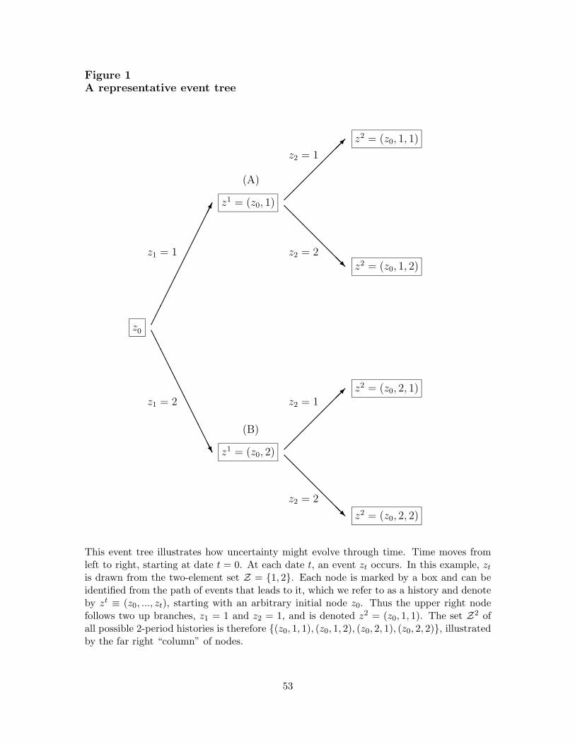
Figure 1A representative event tree

z0

z1 = (z0, 1)

z1 = (z0, 2)

z2 = (z0, 1, 1)

z2 = (z0, 1, 2)

z2 = (z0, 2, 1)

z2 = (z0, 2, 2)

���������������

AAAAAAAAAAAAAAU

��

��

����

@@

@@

@@@R

��

��

����

@@

@@

@@@R

z1 = 1

z1 = 2

z2 = 1

z2 = 2

z2 = 1

z2 = 2

(A)

(B)

This event tree illustrates how uncertainty might evolve through time. Time moves fromleft to right, starting at date t = 0. At each date t, an event zt occurs. In this example, zt

is drawn from the two-element set Z = {1, 2}. Each node is marked by a box and can beidentified from the path of events that leads to it, which we refer to as a history and denoteby zt ≡ (z0, ..., zt), starting with an arbitrary initial node z0. Thus the upper right nodefollows two up branches, z1 = 1 and z2 = 1, and is denoted z2 = (z0, 1, 1). The set Z2 ofall possible 2-period histories is therefore {(z0, 1, 1), (z0, 1, 2), (z0, 2, 1), (z0, 2, 2)}, illustratedby the far right “column” of nodes.

53

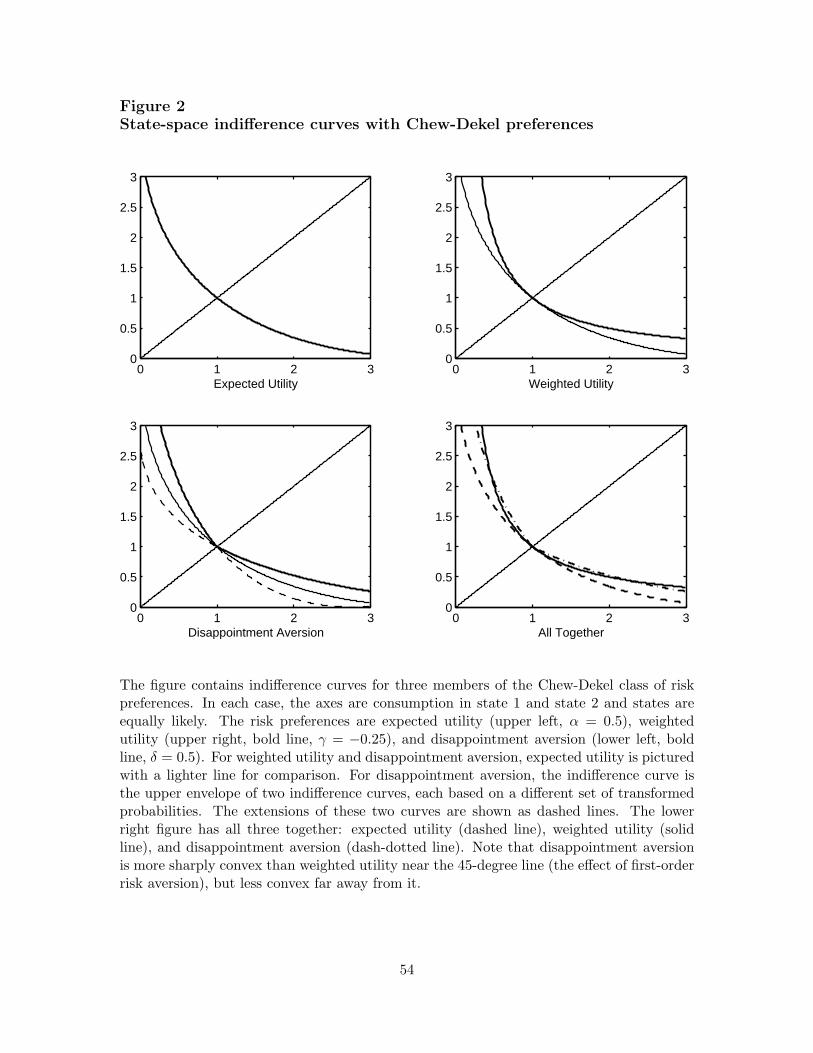
Figure 2State-space indifference curves with Chew-Dekel preferences

0 1 2 30

0.5

1

1.5

2

2.5

3

Expected Utility0 1 2 3

0

0.5

1

1.5

2

2.5

3

Weighted Utility

0 1 2 30

0.5

1

1.5

2

2.5

3

Disappointment Aversion0 1 2 3

0

0.5

1

1.5

2

2.5

3

All Together

The figure contains indifference curves for three members of the Chew-Dekel class of riskpreferences. In each case, the axes are consumption in state 1 and state 2 and states areequally likely. The risk preferences are expected utility (upper left, α = 0.5), weightedutility (upper right, bold line, γ = −0.25), and disappointment aversion (lower left, boldline, δ = 0.5). For weighted utility and disappointment aversion, expected utility is picturedwith a lighter line for comparison. For disappointment aversion, the indifference curve isthe upper envelope of two indifference curves, each based on a different set of transformedprobabilities. The extensions of these two curves are shown as dashed lines. The lowerright figure has all three together: expected utility (dashed line), weighted utility (solidline), and disappointment aversion (dash-dotted line). Note that disappointment aversionis more sharply convex than weighted utility near the 45-degree line (the effect of first-orderrisk aversion), but less convex far away from it.

54

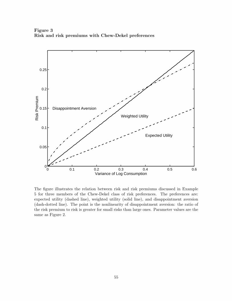
Figure 3Risk and risk premiums with Chew-Dekel preferences

0 0.1 0.2 0.3 0.4 0.5 0.60

0.05

0.1

0.15

0.2

0.25

Variance of Log Consumption

Ris

k P

rem

ium

Expected Utility

Disappointment Aversion

Weighted Utility

The figure illustrates the relation between risk and risk premiums discussed in Example5 for three members of the Chew-Dekel class of risk preferences. The preferences are:expected utility (dashed line), weighted utility (solid line), and disappointment aversion(dash-dotted line). The point is the nonlinearity of disappointment aversion: the ratio ofthe risk premium to risk is greater for small risks than large ones. Parameter values are thesame as Figure 2.

55

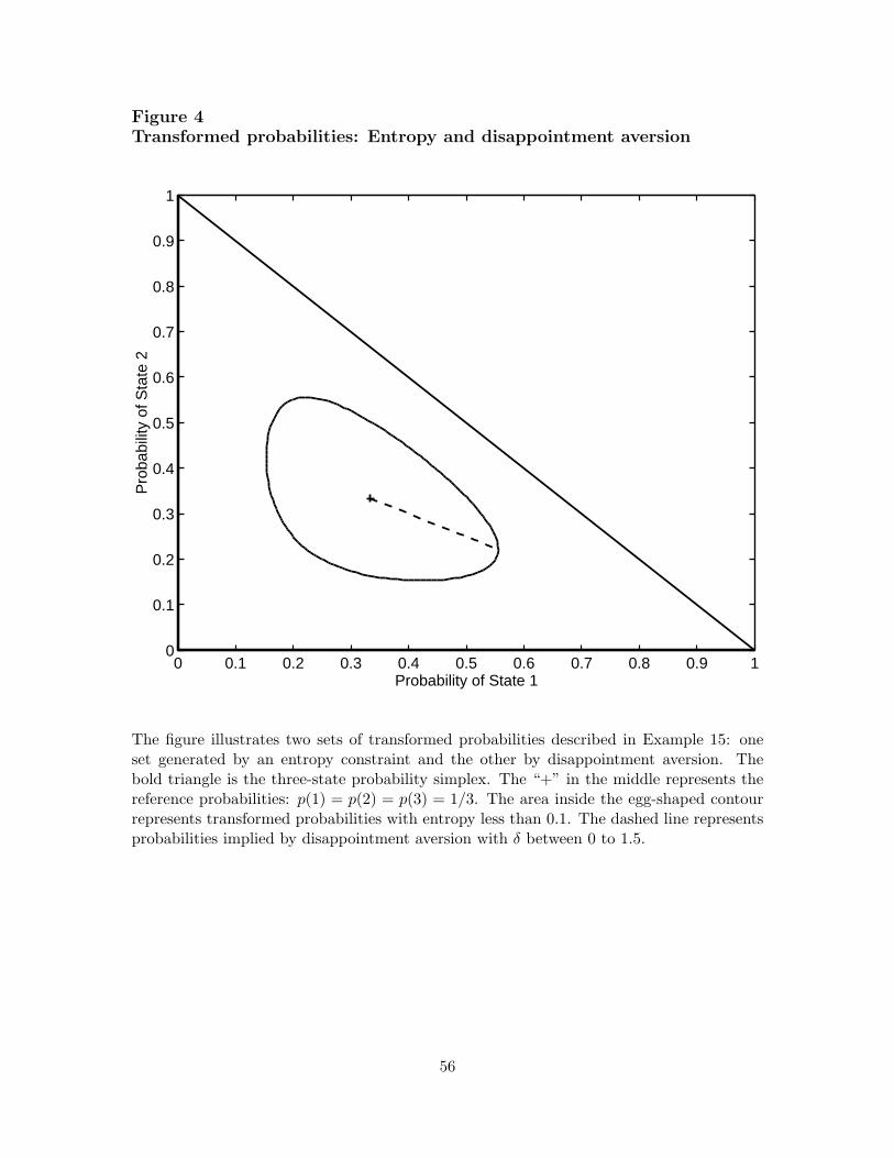
Figure 4Transformed probabilities: Entropy and disappointment aversion

0 0.1 0.2 0.3 0.4 0.5 0.6 0.7 0.8 0.9 10

0.1

0.2

0.3

0.4

0.5

0.6

0.7

0.8

0.9

1

Probability of State 1

Pro

babi

lity

of S

tate

2

The figure illustrates two sets of transformed probabilities described in Example 15: oneset generated by an entropy constraint and the other by disappointment aversion. Thebold triangle is the three-state probability simplex. The “+” in the middle represents thereference probabilities: p(1) = p(2) = p(3) = 1/3. The area inside the egg-shaped contourrepresents transformed probabilities with entropy less than 0.1. The dashed line representsprobabilities implied by disappointment aversion with δ between 0 to 1.5.

56