exeter 2014 bbn_pdf

A multi-dimensional covariance model to combine and interpolate Sea Surface Salinity with Sea Surface

Temperature

Bruno Buongiorno Nardelli, Riccardo Droghei, Lia Santoleri Consiglio Nazionale delle Ricerche-Italia

OUTLINE

OUTLINE

Background on optimal interpolation, state vectors and covariance models

OUTLINE


Algorithm combining in situ/SMOS SSS and satellite SST to get mesoscale resolving SSS

OUTLINE



Choice and preparation of input observations and background data

OUTLINE


Algorithm combining in situ/SMOS SSS and satellite SST to get mesoscale resolving SSS Choice and preparation of input

observations and background data

CAL/VAL approach and preliminary results

OUTLINE



Choice and preparation of input observations and background data

CAL/VAL approach and preliminary results

Conclusions and way forward

xanalysis = xbackground +C(R+C)−1(yobs. −xbackground )

Optimal Interpolation, state vectors and covariance models

Optimal estimate of a state vector is obtained from linear combination of observations as:

with:

C =E εbεbT}{ =E (xbackground −xtrue)(xbackground −xtrue)

T}{

R =E εoεoT}{ =E (yobs. −xtrue)(yobs. −xtrue)

T}{

xyobs.

observation error covariance matrix

background error covariance matrix




with:

R accounts for different observations accuracy/representativeness !crucial parameter for combining insitu and satellite data observations


T}{


T}{

xyobs.






with:

choice of the state vector and error covariance models are intimately linked and hide assumptions on the physics


T}{


T}{

xyobs.




Maximum likelihood estimator of Covariance matrix

Sample state vector Data matrix


Maximum likelihood estimator of Covariance matrix

•  Huge amount of satellite data makes this approach impractical •  Most systems based on pre-determined (analytical) covariance functions

and simplifying assumptions

Sample state vector Data matrix

C=C(Δr) Covariance function

Δr = separation between sample elements


State vector choice and corresponding covariance model

Background error covariance matrix only describes SPATIAL variability, 2D covariance function

Single parameter, single snapshot

C=C(Δx, Δy)


State vector choice and corresponding covariance model

Background error covariance matrix only describes SPATIAL variability, 2D covariance function

Single parameter, single snapshot

Single parameter, temporal sequence

Background error covariance matrix includes information on TEMPORAL and SPATIAL variability, 3D covariance function

C=C(Δx, Δy)

C=C(Δx, Δy,Δt)


Multivariate State vectors lead to complex covariance models

multiple parameters, temporal sequence

Background error covariance matrix includes information on TEMPORAL and SPATIAL variability and relations with other parameters !multi-dimensional covariance function

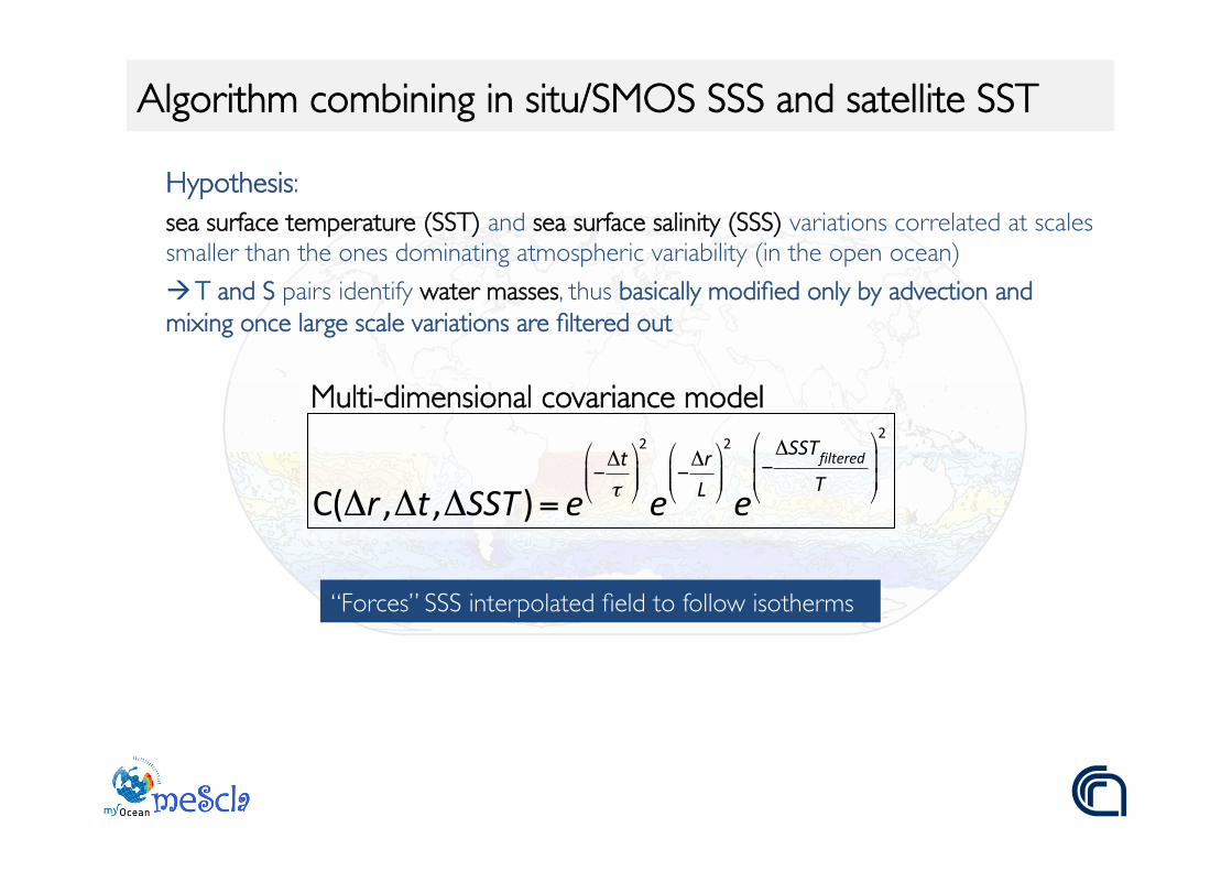
Multi-dimensional covariance model

Algorithm combining in situ/SMOS SSS and satellite SST

Hypothesis: sea surface temperature (SST) and sea surface salinity (SSS) variations correlated at scales smaller than the ones dominating atmospheric variability (in the open ocean) à T and S pairs identify water masses, thus basically modified only by advection and mixing once large scale variations are filtered out

C(Δr ,Δt,ΔSST )= e−Δtτ

#

$%%

&

'((

2

e−ΔrL

#

$%%

&

'((

2

e−ΔSSTfiltered

T

#

$

%%

&

'

((

2




#

$%%

&

'((

2

e−ΔrL

#

$%%

&

'((

2

e−ΔSSTfiltered

T

#

$

%%

&

'

((

2

satellite (spatially high-pass filtered) SST differences are included in the covariance estimation





#

$%%

&

'((

2

e−ΔrL

#

$%%

&

'((

2

e−ΔSSTfiltered

T

#

$

%%

&

'

((

2

“Forces” SSS interpolated field to follow isotherms





#

$%%

&

'((

2

e−ΔrL

#

$%%

&

'((

2

e−ΔSSTfiltered

T

#

$

%%

&

'

((

2

spatial (L), temporal (τ) and thermal (T) decorrelation scales and spatial filtering) determined empirically minimizing OI errors vs independent surface observations

•  Buongiorno Nardelli, B., 2012: A Novel Approach for the High-Resolution Interpolation of In Situ Sea Surface Salinity. J. Atmos. Ocean. Technol., 29, 867–879, doi:10.1175/JTECH-D-11-00099.1.

•  Buongiorno Nardelli, B., et al., 2012: Towards high resolution mapping of 3-D mesoscale dynamics from observations, Ocean Sci., 8, 885-901, doi:10.5194/os-8-885-2012, 2012.

•  Buongiorno Nardelli B., 2013: Vortex waves and vertical motion in a mesoscale cyclonic eddy, J. Geophys. Res., 118, 5609–5624, doi:10.1002/jgrc.20345.


Input observations and background data

OI spatial domain and space-time resolution: Southern Ocean (10°-65° S), resolution 1/4°x1/4°, daily SSS: ISAS/CORA4.0 optimally interpolated SSS (insitu, space-time cov.) (1/2°, monthly) background Quality controlled insitu SSS used for MyOcean CORA4.0 objective analysis input SMOS - BEC Reprocessed L3 mixed (1/4°, 3days) input SST: Reynolds Optimally Interpolated SST from insitu/infrared/microwave data (1/4°, daily) input


Insitu (1 month) SMOS (3 days)


SMOS - BEC Reprocessed L3 mixed (1/4°, 3days) àlarge scale bias àsmall scale noise


SMOS - BEC Reprocessed L3 mixed (1/4°, 3days) !large scale bias: estimated vs CORA4 and removed (5°x5°moving avg.) àsmall scale noise


SMOS - BEC Reprocessed L3 mixed (1/4°, 3days) !large scale bias: estimated vs CORA4 and removed (5°x5°moving avg.) àsmall scale noise: filtered through outlier detection procedure |SMOS-CORA4| <σ(SMOS-CORA4) |SMOS-SMOSsmooth| <σ(SMOS-SMOSsmooth) (1°x1°moving avg.)

CAL/VAL approach

Tuning of SMOS error covariance values (expressed as noise-to-signal ratio) !run OI* with different noise-to-signal values for SMOS (between .5 and 3.) àcompute statistics of differences between OI SSS and independent ThermoSalinoGraph (TSG) data, and between OI SSS gradient and gradients estimated from TSG data àfind best configuration (minimum RMS errors) *Space/Time/Thermal decorrelation scales and insitu noise-to-signal ratio taken from previous studies.

CAL/VAL approach

Preliminary analysis carried out only on 5 days, selected looking at TSG matchup distribution (2-6 January 2012)

Tuning of SMOS error covariance values (expressed as noise-to-signal ratio) !run OI* with different noise-to-signal values for SMOS (between .5 and 3.) àcompute statistics of differences between OI SSS and independent ThermoSalinoGraph (TSG) data, and between OI SSS gradient and gradients estimated from TSG data àfind best configuration (minimum RMS errors) *Space/Time/Thermal decorrelation scales and insitu noise-to-signal ratio taken from previous studies.

Examples of OI SSS with different configurations

Background

OI SSS built from insitu/SST


OI SSS built from SMOS/SST (noise-to-signal=0.5)


OI SSS built from insitu/SMOS/SST (noise-to-signal=0.5)


OI SSS built from insitu/SMOS/SST (noise-to-signal=1.)


CAL/VAL statistics (preliminary results)

Daily TSG matchup data (all)

(noise-to-signal=2.0) (noise-to-signal=0.5)


RMSE SSS insitu/SMOS/SST = 0.38 ± 0.01 RMSE SSS SMOS/SST = 0.361 ± 0.009 RMSE SSS insitu/SST = 0.283 ± 0.007 RMSE CORA4 = 0.41 ± 0.01 RMSE SSS grad. insitu/SMOS/SST = 0.00209 ± 9. e-05 RMSE SSS grad. SMOS/SST = 0.00205 ± 8. e-05 RMSE SSS grad. insitu/SST = 0.00214 ± 9. e-05 RMSE CORA4 grad. = 0.00226 ± 9. e-05

Confidence intervals estimated through bootstrapping

Daily TSG matchup data (only open ocean)



RMSE SSS insitu/SMOS/SST = 0.137 ± 0.002 RMSE SSS SMOS/SST = 0.211 ± 0.005 RMSE SSS insitu/SST = 0.136 ± 0.004 RMSE CORA4 = 0.148 ± 0.002 RMSE SSS grad. insitu/SMOS/SST = 0.00213 ± 9. e-05 RMSE SSS grad. SMOS/SST = 0.00206 ± 8. e-05 RMSE SSS grad. insitu/SST = 0.00215 ± 9. e-05 RMSE CORA4 grad. = 0.00228 ± 9. e-05



TSG matchup data (only open ocean, within ± 6h nominal SST @me)



RMSE SSS insitu/SMOS/SST = 0.128 ± 0.003 RMSE SSS SMOS/SST = 0.201 ± 0.006 RMSE SSS insitu/SST = 0.131 ± 0.003 RMSE CORA4 = 0.145 ± 0.003 RMSE SSS grad. insitu/SMOS/SST = 0.00169 ± 9. e-05 RMSE SSS grad. SMOS/SST = 0.00178 ± 9. e-05 RMSE SSS grad. insitu/SST = 0.00170 ± 9. e-05 RMSE CORA4 grad. = 0.0019 ± 0.0001



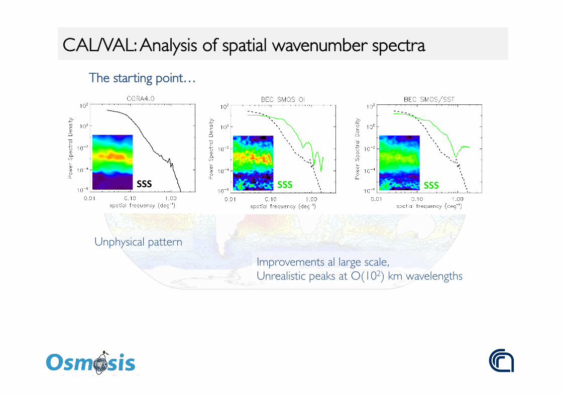
CAL/VAL: Analysis of spatial wavenumber spectra

Mean spatial power spectral density computed from gap/land free sub-images •  de-trended samples •  Blackmann-Harris windowing to reduce spectral leakage •  FFT


Mean zonal power spectral density computed from gap/land free sub-images •  de-trended samples •  Blackmann-Harris windowing to reduce spectral leakage •  FFT


SSS

SSS

SSS

The starting point…

Unphysical pattern Improvements al large scale, Unrealistic peaks at O(102) km wavelengths



SST SSS

SST SSS

SST SSS

SSS

SSS

SSS

Existing vs new products



SST SSS

SST SSS

SST SSS

SST SSS

What should we expect…

Same computation applied to 1/4° ocean model reanalysis CGLORS (assimilating SST, altimeter, in situ)

Conclusions and way forward

Combination/interpolation of insitu/SMOS/SST data using new multi-dimensional covariance model appears promising Need to optimize filtering of SMOS data, include Aquarius/SAC-D CAL/VAL of optimal interpolation configuration needs to be extended to longer dataset Produce/disseminate full processed OSMOSIS dataset (2010-2012, daily resolution, one file per week) Find a framework/project to go global, NRT, daily…

exeter 2014 bbn_pdf

Science

optimal interpolation

xtrue yobs

covariance modelsxoptimal

covariance modelsoptimal

error covariance models

e ooxyobs

xbackground cr c1yobs

situsmos sss andsatellite