exercises in advanced risk and portfolio management · electronic copy available at: 1447443...
TRANSCRIPT

Electronic copy available at: http://ssrn.com/abstract=1447443
Exercises in Advanced Risk and Portfolio Managementwith Step-by-Step Solutions and Fully Documented Code
Attilio [email protected]
This version: August 15 2010Last version available at http://ssrn.com/abstract=1447443
Exercises and case studies for a rigorous approach to risk- and portfolio-management.These exercises stem from the review sessions of the six-day Advanced Risk andPortfolio Management bootcamp http://www.baruch.edu/math/arpm.
Solutions code at http://www.mathworks.com/matlabcentral/fileexchange/25010.Contents include• Advanced multivariate statistics; copula-marginal decomposition• Annualization/projection (FFT, cumulants, simulations)• Pricing: exact; first order (delta/duration); second order (gamma/convexity)• Quest for invariance (stationarity, volatlity clustering, cointegration)• Mutlivariate estimation- Non-parametric; MLE; shrinkage; random matrices; robust; Bayesian;missing data- Generalized hypothesis testing
• Dimension reduction- Statistical (principal components; factor analysis)- Cross-sectional / time-series factor models- Factors on Demand
• Risk management- VaR/CVaR (marginal Euler decomposition; extreme value theory; Cornish-Fisher; elliptical)- Generalized objectives (p&l, return, relative return, etc)- Stochastic dominance/utility theory
• Classical portfolio management: mean-variance• Dynamic strategies (option replication, CPPI, utlity maximization)• Advanced portfolio management- Robust optimization- Black-Litterman and beyond, fully flexible views
1The author is very grateful to Sridhar Gollamudi, Tai-Ho Wang, Colin Rowat, and XiaoyuWang for their help
1
Electronic copy available at: http://ssrn.com/abstract=1447443
Contents1 Distributions 61.1 General . . . . . . . . . . . . . . . . . . . . . . . . . . . . . . . . 6
1.1.1 Invertible transformation of a random variable . . . . . . 61.1.2 Affine transformation of a random variable . . . . . . . . 61.1.3 Sum of random variables: characteristic function . . . . . 71.1.4 Sum of random variables: simulations . . . . . . . . . . . 71.1.5 Fourier transformation . . . . . . . . . . . . . . . . . . . . 81.1.6 Convolution . . . . . . . . . . . . . . . . . . . . . . . . . . 81.1.7 Raw moments to central moments . . . . . . . . . . . . . 91.1.8 Central moments to raw moments . . . . . . . . . . . . . 9
1.2 Parametric . . . . . . . . . . . . . . . . . . . . . . . . . . . . . . 101.2.1 Normal . . . . . . . . . . . . . . . . . . . . . . . . . . . . 101.2.2 Normal moments . . . . . . . . . . . . . . . . . . . . . . . 111.2.3 Normal multivariate with matching moments . . . . . . . 121.2.4 Student t . . . . . . . . . . . . . . . . . . . . . . . . . . . 141.2.5 Lognormal . . . . . . . . . . . . . . . . . . . . . . . . . . 151.2.6 Lognormal moments . . . . . . . . . . . . . . . . . . . . . 161.2.7 Gamma versus chi-square . . . . . . . . . . . . . . . . . . 161.2.8 Wishart simulations . . . . . . . . . . . . . . . . . . . . . 17
1.3 Special classes . . . . . . . . . . . . . . . . . . . . . . . . . . . . . 181.3.1 Empirical . . . . . . . . . . . . . . . . . . . . . . . . . . . 181.3.2 Order statistics . . . . . . . . . . . . . . . . . . . . . . . . 181.3.3 Elliptical variables: radial-uniform representation . . . . . 181.3.4 Elliptical markets and portfolios . . . . . . . . . . . . . . 19
2 Dependence 192.1 Correlation . . . . . . . . . . . . . . . . . . . . . . . . . . . . . . 19
2.1.1 Normal . . . . . . . . . . . . . . . . . . . . . . . . . . . . 192.1.2 Lognormal . . . . . . . . . . . . . . . . . . . . . . . . . . 202.1.3 Independence versus no correlation . . . . . . . . . . . . . 202.1.4 Correlation and location-dispersion ellipsoid . . . . . . . . 22
2.2 Copula . . . . . . . . . . . . . . . . . . . . . . . . . . . . . . . . . 222.2.1 Normal copula pdf . . . . . . . . . . . . . . . . . . . . . . 222.2.2 Normal copula cdf . . . . . . . . . . . . . . . . . . . . . . 232.2.3 Lognormal copula pdf . . . . . . . . . . . . . . . . . . . . 232.2.4 Normal copula and given marginals . . . . . . . . . . . . . 242.2.5 FX copula-marginal factorization . . . . . . . . . . . . . . 252.2.6 Copula vs correlation . . . . . . . . . . . . . . . . . . . . 252.2.7 Full codependence . . . . . . . . . . . . . . . . . . . . . . 26
2
3 Quest for invariance 263.1 Theory . . . . . . . . . . . . . . . . . . . . . . . . . . . . . . . . . 26
3.1.1 Random walk . . . . . . . . . . . . . . . . . . . . . . . . . 263.1.2 AR(1) . . . . . . . . . . . . . . . . . . . . . . . . . . . . . 263.1.3 Volatility clustering . . . . . . . . . . . . . . . . . . . . . 27
3.2 Empirical . . . . . . . . . . . . . . . . . . . . . . . . . . . . . . . 273.2.1 Equity . . . . . . . . . . . . . . . . . . . . . . . . . . . . . 273.2.2 Fixed income . . . . . . . . . . . . . . . . . . . . . . . . . 283.2.3 Derivatives . . . . . . . . . . . . . . . . . . . . . . . . . . 283.2.4 Cointegration . . . . . . . . . . . . . . . . . . . . . . . . . 28
4 Estimation 294.1 Non-parametric . . . . . . . . . . . . . . . . . . . . . . . . . . . . 29
4.1.1 Estimation of moment-based functional . . . . . . . . . . 294.1.2 Estimation of quantile . . . . . . . . . . . . . . . . . . . . 34
4.2 Maximum likelihood . . . . . . . . . . . . . . . . . . . . . . . . . 344.2.1 Basics . . . . . . . . . . . . . . . . . . . . . . . . . . . . . 344.2.2 MLE for univariate elliptical variables . . . . . . . . . . . 354.2.3 MLE for multivariate Student t distribution . . . . . . . . 37
4.3 Shrinkage . . . . . . . . . . . . . . . . . . . . . . . . . . . . . . . 384.3.1 Location . . . . . . . . . . . . . . . . . . . . . . . . . . . . 384.3.2 Scatter . . . . . . . . . . . . . . . . . . . . . . . . . . . . 384.3.3 Sample covariance and eigenvalue dispersion . . . . . . . . 39
4.4 Random matrix theory . . . . . . . . . . . . . . . . . . . . . . . . 394.4.1 Semi-circular law . . . . . . . . . . . . . . . . . . . . . . . 394.4.2 Marchenko-Pastur limit . . . . . . . . . . . . . . . . . . . 40
4.5 Robust . . . . . . . . . . . . . . . . . . . . . . . . . . . . . . . . . 414.5.1 Influence function of sample mean . . . . . . . . . . . . . 414.5.2 Influence function of sample variance . . . . . . . . . . . . 42
4.6 Bayesian . . . . . . . . . . . . . . . . . . . . . . . . . . . . . . . . 444.6.1 Prior on correlation . . . . . . . . . . . . . . . . . . . . . 444.6.2 Normal-Inverse-Wishart posterior . . . . . . . . . . . . . . 45
4.7 Missing data . . . . . . . . . . . . . . . . . . . . . . . . . . . . . 454.7.1 EM algorithm . . . . . . . . . . . . . . . . . . . . . . . . . 45
4.8 Testing . . . . . . . . . . . . . . . . . . . . . . . . . . . . . . . . . 464.8.1 Sample mean . . . . . . . . . . . . . . . . . . . . . . . . . 464.8.2 p-value analytical . . . . . . . . . . . . . . . . . . . . . . . 474.8.3 t-test, location, analytical . . . . . . . . . . . . . . . . . . 474.8.4 t-test, factor loadings, analytical . . . . . . . . . . . . . . 494.8.5 Generalized t-tests, simulations . . . . . . . . . . . . . . . 52
5 Projection and pricing 535.1 Projection of skewness, kurtosis, and all standardized summary
statistics . . . . . . . . . . . . . . . . . . . . . . . . . . . . . . . . 535.2 Multivariate square-root rule . . . . . . . . . . . . . . . . . . . . 565.3 Stable invariants . . . . . . . . . . . . . . . . . . . . . . . . . . . 57
3
5.4 Equities . . . . . . . . . . . . . . . . . . . . . . . . . . . . . . . . 575.4.1 Random walk (linear vs. compounded returns) . . . . . . 575.4.2 Multivariate GARCH . . . . . . . . . . . . . . . . . . . . 59
5.5 Fixed income . . . . . . . . . . . . . . . . . . . . . . . . . . . . . 605.5.1 Normal invariants . . . . . . . . . . . . . . . . . . . . . . 605.5.2 Student t invariants . . . . . . . . . . . . . . . . . . . . . 62
5.6 Derivatives . . . . . . . . . . . . . . . . . . . . . . . . . . . . . . 64
6 Dimension reduction 656.1 "Pure residual" models: duration/curve attribution . . . . . . . . 656.2 "Time series" or "macroeconomic" factor models . . . . . . . . . 65
6.2.1 Unconstrained time series correlations and r-square . . . . 656.2.2 Unconstrained time series industry factors . . . . . . . . . 676.2.3 Generalized time-series industry factors . . . . . . . . . . 676.2.4 Analysis of residual . . . . . . . . . . . . . . . . . . . . . . 68
6.3 "Cross-section" or "fundamental" factor models . . . . . . . . . . 706.3.1 Unconstrained cross-section correlations and r-square . . . 706.3.2 Unconstrained cross-section industry factors . . . . . . . . 716.3.3 Generalized cross-section industry factors . . . . . . . . . 726.3.4 Comparison cross-section with time-series industry factors 736.3.5 Correlation factors-residual: normal example . . . . . . . 73
6.4 "Statistical" approach: principal component analysis . . . . . . . 746.4.1 Matrix algebra . . . . . . . . . . . . . . . . . . . . . . . . 746.4.2 Location-dispersion ellipsoid and geometry . . . . . . . . 746.4.3 Location-dispersion ellipsoid and statistics . . . . . . . . . 756.4.4 PCA derivation, correlations and r-square . . . . . . . . . 756.4.5 PCA and projection . . . . . . . . . . . . . . . . . . . . . 776.4.6 PCA of two-point swap curve . . . . . . . . . . . . . . . . 776.4.7 Eigenvectors for Toeplitz structure . . . . . . . . . . . . . 776.4.8 Generalized principal component analysis . . . . . . . . . 78
6.5 "Statistical" approach: factor analysis puzzle . . . . . . . . . . . 786.6 "Factors on Demand" . . . . . . . . . . . . . . . . . . . . . . . . 78
6.6.1 Horizon effect . . . . . . . . . . . . . . . . . . . . . . . . . 786.6.2 No-Greek hedging . . . . . . . . . . . . . . . . . . . . . . 806.6.3 Selection heuristics . . . . . . . . . . . . . . . . . . . . . . 81
7 Risk Management 837.1 Investor’s objectives . . . . . . . . . . . . . . . . . . . . . . . . . 83
7.1.1 General . . . . . . . . . . . . . . . . . . . . . . . . . . . . 837.2 Dominance . . . . . . . . . . . . . . . . . . . . . . . . . . . . . . 83
7.2.1 Strong dominance . . . . . . . . . . . . . . . . . . . . . . 837.2.2 Weak dominance . . . . . . . . . . . . . . . . . . . . . . . 84
7.3 Utility . . . . . . . . . . . . . . . . . . . . . . . . . . . . . . . . . 847.3.1 Certainty equivalent interpretation . . . . . . . . . . . . . 847.3.2 Certainty equivalent computation . . . . . . . . . . . . . . 847.3.3 Arrow-Pratt aversion and prospect theory . . . . . . . . . 85
4
7.4 VaR . . . . . . . . . . . . . . . . . . . . . . . . . . . . . . . . . . 867.4.1 VaR in elliptical markets . . . . . . . . . . . . . . . . . . 867.4.2 Cornish-Fisher approximation of VaR . . . . . . . . . . . 897.4.3 Extreme value theory approximation of VaR . . . . . . . 89
7.5 Expected shortfall . . . . . . . . . . . . . . . . . . . . . . . . . . 907.5.1 Expected shortfall in elliptical markets . . . . . . . . . . . 907.5.2 Expected shortfall and linear factor models . . . . . . . . 91
8 Static portfolio management 928.1 Mean-variance . . . . . . . . . . . . . . . . . . . . . . . . . . . . 92
8.1.1 Mean-variance pitfalls: two-step approach . . . . . . . . . 928.1.2 Mean-variance pitfalls: horizon effect . . . . . . . . . . . . 938.1.3 Benchmark driven allocation . . . . . . . . . . . . . . . . 948.1.4 Mean-variance for derivatives . . . . . . . . . . . . . . . . 96
9 Dynamic strategies 969.1 Buy & hold . . . . . . . . . . . . . . . . . . . . . . . . . . . . . . 989.2 Utility maximization . . . . . . . . . . . . . . . . . . . . . . . . . 999.3 Constant proportion portfolio insurance (CPPI) . . . . . . . . . . 1029.4 Option based portfolio insurance (OBPI) . . . . . . . . . . . . . 103
10 Estimation risk 10610.1 General . . . . . . . . . . . . . . . . . . . . . . . . . . . . . . . . 106
10.1.1 Opportunity cost . . . . . . . . . . . . . . . . . . . . . . . 10610.2 Robust . . . . . . . . . . . . . . . . . . . . . . . . . . . . . . . . . 106
10.2.1 Robust mean-variance for derivatives . . . . . . . . . . . . 10610.3 Black-Litterman & beyond . . . . . . . . . . . . . . . . . . . . . . 107
10.3.1 Black-Litterman . . . . . . . . . . . . . . . . . . . . . . . 10710.3.2 Beyond Black-Litterman . . . . . . . . . . . . . . . . . . . 108
References 110
5
1 Distributions
1.1 General
1.1.1 Invertible transformation of a random variable
Consider as in (T1.1) in the Technical Appendices at symmys.com > Book >Downloads the following transformation of the generic random variable X:
X 7→ Y ≡ g (X) , (1)
where g is an increasing and thus invertible function.Prove the following formulas:
FY (y) = FX¡g−1 (y)
¢(2)
fY (y) =fX¡g−1 (y)
¢g0 (g−1 (y))
. (3)
QY (p) = g (QX (p)) (4)
See Section 1.1 in the Technical Appendices. In particular, for the cdf, bythe definition of the cumulative distribution function FY we have:
FY (y) ≡ P {Y ≤ y} = P {g (X) ≤ y}= P
©X ≤ g−1 (y)
ª(5)
= FX¡g−1 (y)
¢.
For the pdf, by derivation of both sides the above result we obtain:
fY (y) =fX¡g−1 (y)
¢g0 (g−1 (y))
(6)
For the quantile, as in the Technical Appendices consider the following series ofidentities:
FY (g (QX (p))) = P {Y ≤ g (QX (p))} = P {X ≤ QX (p)} = p, (7)
By applying the definition of the quantile QY to the above terms we obtain:
QY (p) = g (QX (p)) , (8)
1.1.2 Affine transformation of a random variable
Consider as in (T1.12) in the Technical Appendices the following positive affinetransformation of the generic random variable X:
X 7→ Y ≡ g (X) ≡ m+ sX, (9)
6
where s > 0 and m is a generic constant.Prove the following formulas:
fY (y) =1
sfX
µy −m
s
¶(10)
FY (y) = FX
µy −m
s
¶(11)
QY (p) = m+ sQX (p) (12)
φY (ω) = eiωmφX (sω) (13)
See Section 1.2 in the Technical Appendices.
1.1.3 Sum of random variables: characteristic function
Consider the random variable defined in distribution as
Xd≡ Y + Z, (14)
where Y and Z are independent.Compute the characteristic function φX of X from the characteristic func-
tions φY of Y and φZ of Z.
φX (ω) ≡ E©eiωX
ª= E
neiω(Y+Z)
o= E
©eiωY eiωZ
ª(15)
= E©eiωY
ªE©eiωZ
ª= φY (ω)φZ (ω)
1.1.4 Sum of random variables: simulations
Consider a Student t-distributed random variable
X ∼ St¡ν, µ, σ2
¢, (16)
where ν ≡ 8, µ ≡ 0 and σ2 ≡ 0.1. Consider an independent lognormal randomvariable
Y ∼ LogN¡µ, σ2
¢, (17)
where µ ≡ 0.1 and σ2 ≡ 0.2. Consider the random variable defined as
Z ≡ X + Y . (18)
Generate the script S_NonAnalytical in which you perform the following op-erations.Generate a large (≈ 10, 000 observations) sample X from (16), a sample Y of
equal size from (17), sum them term by term (do not use loops) and obtain alarge sample Z from (18).
7
Plot the sample Z. Do not join the observations (use the plot option ’.’ asin a scatterplot).Plot the histogram of Z. Use hist and choose the number of bins appropri-
ately.Plot the empirical cdf of Z. Use [f,z]=ecdf(Z) and plot(z,f).Plot the empirical quantile of Z. Use prctile.
See the script S_NonAnalytical.
1.1.5 Fourier transformation
Prove that the Fourier transformation (B.34) in Meucci (2005) is a linear oper-ator, i.e. it satisfies (B.24).
From the definition (B.34)
F [u+ v] (y) ≡ZRN
eiy0x (u (x) + v (x)) dx (19)
=
ZRN
eiy0xu (x) dx+
ZRN
eiy0xv (x) dx
≡ F [u] (y) + F [v] (y)
Also, from the definition (B.34)
F [αv] ≡ZRN
eiy0x (αv (x)) dx (20)
= α
ZRN
eiy0xv (x) dx ≡ αF [v]
Therefore (B.24) is satisfied.
1.1.6 Convolution
Prove that the convolution (B.43) in Meucci (2005) of two probability densityfunctions is a probability density function.
Consider probability density functions f and h, i.e. two functions that satisfy(2.5)-(2.6). Consider their convolution g ≡ f ∗ h, which from the definition(B.43) reads explicitly:
g (x) ≡ZRN
f (y)h (x− y) dy. (21)
8
Property (2.5) is satisfied because f and h are non-negative. As for (2.6)ZRN
g (x) dx ≡ZRN
µZRN
f (y)h (x− y) dy¶dx (22)
=
ZRN
f (y)
µZRN
h (x− y) dx¶dy
=
ZRN
f (y) dy = 1,
where in the second to last row we used a change of variables x→ z ≡ x− y.
1.1.7 Raw moments to central moments
Consider the raw moments (1.47)
eµ(n)X ≡ E{Xn}, n = 1, 2, . . . ; (23)
and the central moments (1.48)
µ(1)X ≡ µX ≡ eµ(1)X ; µ
(n)X ≡ E{(X − µX)
n}, n = 2, 3, . . . . (24)
Create a function Raw2Central that maps the first n raw moments into the firstn central moments.
See function Raw2Central.For n > 1, from the definition of central moment (24) and the binomial
expansion we obtain
µ(n)X ≡ E{(X − µX)
n}
= E
(n−1Xk=0
(−1)n−k µn−kX Xk +Xn
)(25)
=n−1Xk=0
(−1)n−k µn−kX E©Xkª+E {Xn}
=n−1Xk=0
(−1)n−k µn−kX eµ(k)X + eµ(n)X .
1.1.8 Central moments to raw moments
Consider the raw moments (1.47) in Meucci (2005)
eµ(n)X ≡ E{Xn}, n = 1, 2, . . . ; (26)
9

and the central moments (1.48) in Meucci (2005)
µ(1)X ≡ µX ≡ eµ(1)X ; µ
(n)X ≡ E{(X − µX)
n}, n = 2, 3, . . . . (27)
Create a function Central2Raw that maps the first n central moments into thefirst n raw moments.
See function Central2Raw.From (25) we obtain
eµ(n)X = µ(n)X +
n−1Xk=0
(−1)n−k+1 µn−kX eµ(k)X .
This is a recursive formula that we initiate as eµ(1)X = µ(1)X , which follows from
(27).
1.2 Parametric
1.2.1 Normal
Consider as in (1.66) in Meucci (2005) a normal random variable
X ∼ N¡µ, σ2
¢. (28)
Generate the script S_NormalSample in which you perform the following oper-ations. Compute µ and σ2 such that E {X} ≡ 3 and Var {X} ≡ 5.
From (1.71) E {X} = µ and from (1.72) Var {X} = σ2. Notice that theMATLAB built-in functions take µ and
√σ2 as inputs.
Generate a large (≈ 10, 000 observations) sample X from this distributionusing normrnd.In Figure 1, plot the sample. Do not join the observations (use the plot
option ’.’ as in a scatterplot).In Figure 2, plot the histogram. Use hist and choose the number of bins
appropriately.In Figure 3, plot the empirical cdf. Use [f,x]=ecdf(X) and plot(x,f).Superimpose (use hold on) the exact cdf as computed by normcdf. Use a
different color.In Figure 4, plot the empirical quantile. Use prctile.Superimpose (use hold on) the exact quantile as computed by norminv. Use
a different color.
See the script S_NormalSample.
10
1.2.2 Normal moments
Compute the central moments
µ(n)X ≡ E {(X − E {X})n} (29)
of a normal distributionX ∼ N
¡µ, σ2
¢. (30)
For a generic random variable X, the moment generating function
MX (z) ≡Z
ezxfX (x) dx (31)
is such that DnMX (0) = eµ(n)X , where D is the derivation operator and
eµ(n)X ≡ E {Xn} (32)
is the non-central moment. This follows from explicitly applying D on bothsides of (31). The moment generating function is the characteristic functionφX (ω) defined in (1.12) in Meucci (2005) evaluated at ω ≡ z/i
MX (z) = φX (z/i) . (33)
First we focus on the non-central moments of the standard normal distrib-ution
Y ∼ N(0, 1) . (34)
From (1.69) in Meucci (2005) and (33) we obtain MY (z) ≡ ez2/2. Computing
the derivatives
D0MY (z) = ez2/2
D1MY (z) = ze12 z
2
D2MY (z) = e12z
2
+ z2e12z
2
D3MY (z) = z3e12z
2
+ 3ze12 z
2
(35)
D4MY (z) = 3e12z
2
+ 6z2e12z
2
+ z4e12z
2
D5MY (z) = 10z3e12z
2
+ z5e12z
2
+ 15ze12 z
2
D6MY (z) = 15e12z
2
+ 45z2e12z
2
+ 15z4e12z
2
+ z6e12z
2
...
and evaluating in zero yields the result
eµ(n)Y =
½0 if n is odd(n− 1)!! if n is even,
(36)
where n!! ≡ 1× 3× 5× · · · × n.
11
Now we notice thatµ(n)X = eµ(n)X−µ (37)
which follows from (29), (32) and (1.71) in Meucci (2005). Furthermore
eµ(n)X−µ = σneµ(n)Y (38)
because X − µd= σY , as follows form (2.163) in Meucci (2005) applied to the
univariate case. Therefore
µ(n)X =
½0 if n is oddσn (n− 1)!! if n is even
(39)
1.2.3 Normal multivariate with matching moments
This exercise is discussed in greater depth and placed into a broader context inMeucci (2009c), freely available online at ssrn.com, which we follow below.Consider as in (2.155) in Meucci (2005) a mutlivariate normal market
X ∼ N(µ,Σ) , (40)
where µ and Σ are arbitrary.Generate a large number of scenarios {xj}j=1,...,J from the distribution (40)
in such a way that the sample mean and covariance
bµ ≡ 1
J
JXj=1
xj , bΣ ≡ 1
J
JXj=1
(xj − µ) (xj − µ)0 (41)
satisfy bµ ≡ µ bΣ ≡ Σ. (42)
Hint. If you need to solve a Riccati equation
Σ ≡ BbΣB, B ≡ B0. (43)
you can follow Petkov, Christov, and Konstantinov (1991). First define theHamiltonian matrix
H ≡µ
0 −bSy−S 0
¶. (44)
Next perform its Schur decomposition
H ≡ UTU0, (45)
where UU0 ≡ I and T is upper triangular with the eigenvalues of H on thediagonal sorted in such a way that the first N have negative real part and theremaining N have positive real part; the terms in this decomposition are similar
12

in nature to principal components and are computed by MATLAB. Then thesolution of the Riccati equation (43) reads
B ≡ ULLU−1UL, (46)
where UUL is the upper left N ×N block of U and ULL is the lower left N ×Nblock of U.
population moments
-0 .8 -0.6 -0.4 -0.2 0 0.2 0.4 0.6 0.8
-0.5
-0.4
-0.3
-0.2
-0.1
0
0.1
0.2
0.3
0.4
0.5
-0.8 -0.6 -0.4 -0.2 0 0.2 0.4 0.6 0.8
-0.5
-0.4
-0.3
-0.2
-0.1
0
0.1
0.2
0.3
0.4
0.5
sample moments
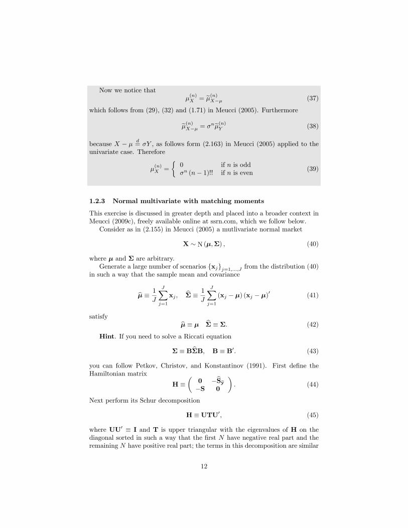
standard simulation proposed approach
Figure 1: Sample and population moments coincide our approach
See the function MvnRnd, which takes the same inputs and yields the sameoutput as the built-in MATLAB function mvnrnd.First produce an auxiliary set of scenarios
{eyj}j=1,..., J2 (47)
from the distribution N(0,Σ). Then complement these scenarios with theiropposite eyj ≡ ½ eyj if 1 ≤ j ≤ J/2
−eyj− J2
if J/2 + 1 ≤ j ≤ J . (48)
These antithetic variables still represent the distribution N(0,Σ), but they aremore efficient they satisfy the zero-mean condition.Next apply a linear transformation to the scenarios eyj , which again preserves
normality:yj ≡ Beyj, j = 1, . . . , J . (49)
For any choice of the invertible matrix B, the sample mean is null. To determineB we impose that the sample covariance matches the desired covariance. Usingthe affine equivariance of the sample covariance which follows from (4.42), (4.36),(2.67) and (2.64) in Meucci (2005), we obtain the matrix Riccati equation (43).
13
With the solution (46) we can perform the affine transformation (49) andfinally generate the desired scenarios
xj ≡ µ+ yj , j = 1, . . . , J , (50)
which satisfy (42), see Figure 1, where as in Meucci (2005) we represent the firsttwo moments of a distribution in terms of an ellipsoid.
1.2.4 Student t
Generate the script S_StudentTSample in which you perform the following op-erations.Consider a Student t random variable
X ∼ St¡ν, µ, σ2
¢. (51)
Knowing that σ2 ≡ 6, compute ν and µ such that E {X} ≡ 2 and Var {X} ≡7. (Note: there is a typo in (1.90) in Meucci (2005). Check the "Errata" atsymmys.com > Book > Downloads).Generate a sample X_a of T ≡ 10, 000 observations from (51) using the
built-in t number generator.Generate a sample X_b of T ≡ 10, 000 observations from (51) using the
normal number generator, the chi-square number generator and the followingresult:
Xd= µ+
YpZ/ν
, (52)
where Y and Z are independent variables distributed as follows:
Y ∼ N¡0, σ2
¢, Z ∼ χ2ν . (53)
Generate a sample X_c of T ≡ 10, 000 observations from (51) using theuniform generator number, tinv and (2.27) in Meucci (2005).In a separate figure, subplot the histogram of the simulations of X_a,
subplot the histogram of the simulations of X_b and subplot the histogram ofthe simulations of X_c.Compute the empirical quantile functions of the three simulations corre-
sponding to the confidence grid
G ≡ {0.01, 0.02, . . . , 0.99} (54)
In a separate figure superimpose the plots of the above empirical quantiles,which should coincide. Use different colors.
See the script S_StudentTSample.
14
1.2.5 Lognormal
Consider as in (1.94) in Meucci (2005) a lognormal random variable
X ∼ LogN¡µ, σ2
¢. (55)
Generate the script S_LognormalSample in which you perform the followingoperations.Compute µ and σ2 such that E {X} ≡ 3 and Var {X} ≡ 5.
From (1.98) and (1.99) we need to solve for µ and σ2 the following system:
E = eµ+σ2
2 (56)
V = e2µ+σ2³eσ
2 − 1´
(57)
or
2 ln (E) = 2µ+ σ2 (58)
ln (V ) = 2µ+ σ2 + ln³eσ
2 − 1´
(59)
Therefore
ln
µV
E2
¶= ln
³eσ
2 − 1´
(60)
or
σ2 = ln
µ1 +
V
E2
¶. (61)
From (58) we then obtain:
µ = ln (E)− 12ln
µ1 +
V
E2
¶. (62)
Notice that the MATLAB built-in functions take µ and√σ2 as inputs.
Generate a large (≈ 10, 000 observations) sample X from this distributionusing lognrnd.In Figure 1, plot the sample. Do not join the observations (use the plot
option ’.’ as in a scatterplot).In Figure 2, plot the histogram. Use hist and choose the number of bins
appropriately.In Figure 3, plot the empirical cdf. Use [f,x]=ecdf(X) and plot(x,f).Superimpose (use hold on) the exact cdf as computed by logncdf. Use a
different color.In Figure 4, plot the empirical quantile. Use prctile.Superimpose (use hold on) the exact quantile as computed by logninv. Use
a different color.
15
See the script S_LognormalSample.
1.2.6 Lognormal moments
Consider as in (1.94) in Meucci (2005) a lognormal random variable
X ∼ LogN¡µ, σ2
¢. (63)
Compute the raw momentsµn ≡ E {Xn} (64)
for all n = 1, 2, . . .
From (1.94) in Meucci (2005)
Xn d= enY , (65)
whereY ∼ N
¡µ, σ2
¢. (66)
From (2.163) in Meucci (2005)
nY ∼ N¡nµ, n2σ2
¢(67)
ThereforeXn ∼ LogN
¡nµ, n2σ2
¢(68)
and the moments follow from (1.98) in Meucci (2005)
µn = enµ+n2σ2/2 (69)
1.2.7 Gamma versus chi-square
Consider as in (1.107) in Meucci (2005) a gamma-distributed random variable
X ∼ Ga¡ν, µ, σ2
¢. (70)
We recall that such variable is defined in distribution as follows
Xd≡ Y 2
1 + · · ·+ Y 2ν , (71)
whereY1
d≡ · · · d≡ Yν ∼ N¡µ, σ2
¢(72)
are independent. For which values of ν, µ and σ2 does this distribution coincidewith the chi-square distribution with ten degrees of freedom?
16
For ν ≡ 10, µ ≡ 0 and σ2 ≡ 1 we obtain X ∼ χ210, see (1.109) in thetextbook.
1.2.8 Wishart simulations
Consider the case N ≡ 2 of a Wishart distribution
W ∼W(ν,Σ) , (73)
where
Σ ≡µ
σ21 ρσ1σ2ρσ1σ2 σ22
¶. (74)
Fix σ1 ≡ 1 and σ2 ≡ 1. Generate the script S_Wishartwhere you perform thefollowing operations.Set your inputs ρ and ν.Generate a sample of size J ≡ 10, 000 from W(ν,Σ) using the equivalent
stochastic representation (2.222) in Meucci (2005).Positivity implies that D ≡ det (W) and T ≡ tr (W) are positive random
variables, see (2.236), (2.237) in Meucci (2005). Plot the histograms of therealizations of D and T , which are approximations of the respective pdf’s, toshow that indeed these random variables are positive. Comment on whetherthis is also true for ν ≡ 1.Symmetry implies that a matrix is fully determined by the three non-redundant
entries (W11,W22,W12). Plot the 3-d scatter-plot of the realizations of W11 vs.W12 vs. W22 to show the Wishart cloud. Notice that as the degrees of freedomν increases the clouds becomes less and less "wedgy". Eventually, it becomes anormal ellipsoid, in accordance with the central limit theorem.Plot the separate histograms of the realizations of W11, W12 and W22.From (2.230) in Meucci (2005) the marginal distributions of the diagonal
elements of a Wishart matrix are gamma-distributed:
Wnn ∼ Ga (ν,Σnn) . (75)
Superimpose the rescaled pdf (1.110) of the marginals of W11 and W22 tothe respective histograms to show that histogram and gamma pdf coincide, see(T1.43) in the technical appendices at www.symmys.com > Book > DownloadsCompute and show on the command window the sample means, sample
covariances, sample standard deviations and sample correlations.Compute and show on the command window the respective analytical results
(2.227) and (2.228) in Meucci (2005), making sure that they coincide.
See the script S_Wishart.
17
1.3 Special classes
1.3.1 Empirical
Derive expression (2.243) in Meucci (2005) for the characteristic function of theempirical distribution.
φiT (ω) ≡ Eneiω
0Xo=
ZRN
eiω0xfiT (x) dx
=
ZRN
eiω0x
"1
T
TXt=1
δ(xt) (x)
#dx (76)
=1
T
TXt=1
ZRN
eiω0xδ(xt) (x) dx.
Using (B.17) we obtain:
φiT (ω)=1
T
TXt=1
eiω0xt . (77)
1.3.2 Order statistics
Replicate the exercise S_OrderStatisticsPDFStudentTassuming that the i.i.d.variables are lognormal instead of t-distributed.Note. The figure generated by the script is 3-d: make sure to rotate the
figure in order to appreciate the third dimension as in Figure 2.19 in Meucci(2005).
See the script S_OrderStatisticsPDFLogn.
1.3.3 Elliptical variables: radial-uniform representation
Generate a non-trivial 30× 30 symmetric and positive matrix Σ and a 30-dimvector µ.Generate J ≡ 10, 000 simulations from a 30-dimensional elliptical random
variable:X ≡ µ+RAU. (78)
In this expression µ, R, A,U are the terms of the radial-uniform decomposition,see (2.259) in Meucci (2005). In particular, set
R ∼ LogN¡ν, τ2
¢, (79)
where ν ≡ 0.1 and τ2 ≡ 0.04.
18
See the script S_EllipticalNDim.
1.3.4 Elliptical markets and portfolios
Consider an elliptical market
M ∼ El (µ,Σ, gN ) , (80)
Consider the objective Ψα ≡ α0M, where α is a generic vector of exposures.Prove that
Ψαd= µα + σαZ, (81)
whereZ ∼ El (0, 1, g1) . (82)
Write the expression for µα and σα.
From (2.270) in Meucci (2005) we obtain
Ψα ∼ El¡µα, σ
2α, g1
¢, (83)
where
µα ≡ α0µ (84)
σ2α ≡ α0Σα (85)
From (2.258) in Meucci (2005)
Ψαd= µα + σαZ, (86)
where Z is spherically symmetrical and therefore
Z ∼ El (0, 1, g1) . (87)
2 Dependence
2.1 Correlation
2.1.1 Normal
Consider a bivariate normal random variable:µX1
X2
¶∼ N
µµµ1µ2
¶,
µσ21 ρσ1σ2
ρσ1σ2 σ22
¶¶. (88)
Fix µ1 ≡ 0, µ2 ≡ 0, σ1 ≡ 1, σ2 ≡ 1 and generate a script that:plots the correlation between X1 and X2 as a function of ρ ∈ (−1, 1);
19
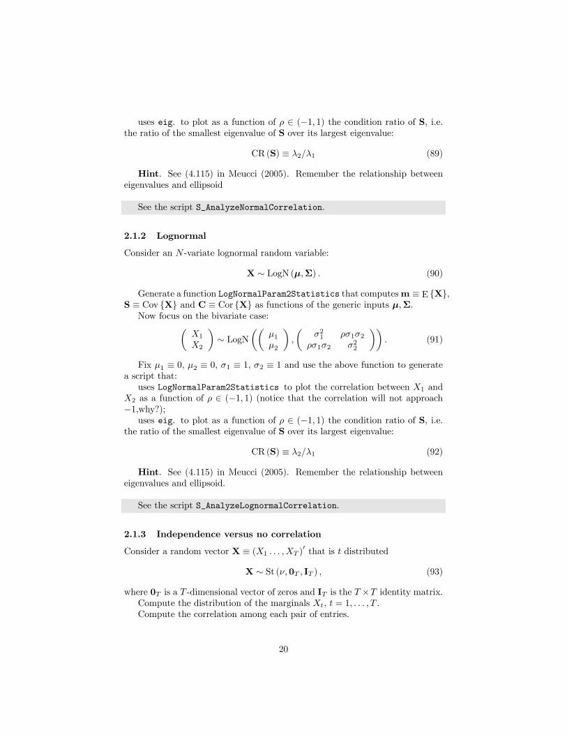
uses eig. to plot as a function of ρ ∈ (−1, 1) the condition ratio of S, i.e.the ratio of the smallest eigenvalue of S over its largest eigenvalue:
CR(S) ≡ λ2/λ1 (89)
Hint. See (4.115) in Meucci (2005). Remember the relationship betweeneigenvalues and ellipsoid
See the script S_AnalyzeNormalCorrelation.
2.1.2 Lognormal
Consider an N -variate lognormal random variable:
X ∼ LogN (µ,Σ) . (90)
Generate a function LogNormalParam2Statistics that computesm ≡ E {X},S ≡ Cov {X} and C ≡ Cor {X} as functions of the generic inputs µ,Σ.Now focus on the bivariate case:µ
X1
X2
¶∼ LogN
µµµ1µ2
¶,
µσ21 ρσ1σ2
ρσ1σ2 σ22
¶¶. (91)
Fix µ1 ≡ 0, µ2 ≡ 0, σ1 ≡ 1, σ2 ≡ 1 and use the above function to generatea script that:uses LogNormalParam2Statistics to plot the correlation between X1 and
X2 as a function of ρ ∈ (−1, 1) (notice that the correlation will not approach−1,why?);uses eig. to plot as a function of ρ ∈ (−1, 1) the condition ratio of S, i.e.
the ratio of the smallest eigenvalue of S over its largest eigenvalue:
CR(S) ≡ λ2/λ1 (92)
Hint. See (4.115) in Meucci (2005). Remember the relationship betweeneigenvalues and ellipsoid.
See the script S_AnalyzeLognormalCorrelation.
2.1.3 Independence versus no correlation
Consider a random vector X ≡ (X1 . . . ,XT )0 that is t distributed
X ∼ St (ν,0T , IT ) , (93)
where 0T is a T -dimensional vector of zeros and IT is the T ×T identity matrix.Compute the distribution of the marginals Xt, t = 1, . . . , T .Compute the correlation among each pair of entries.
20

Compute the distribution of
Y ≡TXt=1
Xt. (94)
Now consider T i.i.d. t-distributed random variables:eXt ∼ St (ν, 0, 1) , t = 1, . . . , T (95)
Compute the correlation among each pair of entries.Consider the limit T →∞ and compute the distribution of
eY ≡ TXt=1
eXt. (96)
Comment on the difference between the distribution of Y versus the distri-bution of eY .From (2.194) in Meucci (2005) the marginals read:
Xt ∼ St (ν, 0, 1) , t = 1, . . . , T . (97)
From (2.191) the cross-correlations read:
Cor {Xt,Xs} = 0, t 6= s. (98)
From (2.195) we obtain
Y ≡TXt=1
Xt = 10X ∼ St (ν,100T ,10IT1) . (99)
ThereforeY ∼ St (ν, 0, T ) . (100)
As far as eX is concerned, from (2.136) the cross-correlations read:
Corn eXt, eXs
o= 0, t 6= s. (101)
From the central limit theorem and (1.90) in Meucci (2005) (fix the typo withthe online "Errata" at symmys.com > Book > Downloads) we obtain:
eY → N
µ0,
ν
ν − 2T¶. (102)
Both Y and eY are the sum of uncorrelated identically distributed t variables.If the variables are independent, the CLT kicks in and the sum becomes
normal. Note: this only holds for ν > 2, otherwise the variance is not definedand the CLT does not hold. Indeed, if ν = 1 we obtain the Cauchy distribution,which is stable: the sum of i.i.d. Cauchy variables is Cauchy. If the variablesare jointly t, they cannot be independent, even if they are uncorrelated, recallthe plot of the pdf of the Student t copula.
21
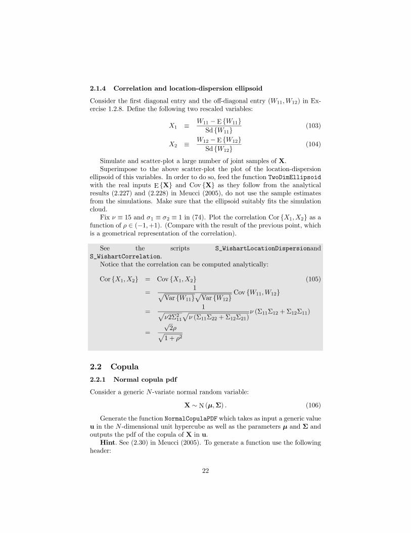
2.1.4 Correlation and location-dispersion ellipsoid
Consider the first diagonal entry and the off-diagonal entry (W11,W12) in Ex-ercise 1.2.8. Define the following two rescaled variables:
X1 ≡ W11 − E {W11}Sd {W11}
(103)
X2 ≡ W12 − E {W12}Sd {W12}
(104)
Simulate and scatter-plot a large number of joint samples of X.Superimpose to the above scatter-plot the plot of the location-dispersion
ellipsoid of this variables. In order to do so, feed the function TwoDimEllipsoidwith the real inputs E {X} and Cov {X} as they follow from the analyticalresults (2.227) and (2.228) in Meucci (2005), do not use the sample estimatesfrom the simulations. Make sure that the ellipsoid suitably fits the simulationcloud.Fix ν ≡ 15 and σ1 ≡ σ2 ≡ 1 in (74). Plot the correlation Cor {X1,X2} as a
function of ρ ∈ (−1,+1). (Compare with the result of the previous point, whichis a geometrical representation of the correlation).
See the scripts S_WishartLocationDispersionandS_WishartCorrelation.Notice that the correlation can be computed analytically:
Cor {X1,X2} = Cov {X1,X2} (105)
=1p
Var {W11}pVar {W12}
Cov {W11,W12}
=1p
ν2Σ211pν (Σ11Σ22 +Σ12Σ21)
ν (Σ11Σ12 +Σ12Σ11)
=
√2ρp1 + ρ2
2.2 Copula
2.2.1 Normal copula pdf
Consider a generic N -variate normal random variable:
X ∼ N(µ,Σ) . (106)
Generate the function NormalCopulaPDF which takes as input a generic valueu in the N -dimensional unit hypercube as well as the parameters µ and Σ andoutputs the pdf of the copula of X in u.Hint. See (2.30) in Meucci (2005). To generate a function use the following
header:
22
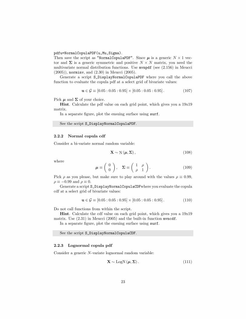
pdfu=NormalCopulaPDF(u,Mu,Sigma).Then save the script as "NormalCopulaPDF". Since µ is a generic N × 1 vec-tor and Σ is a generic symmetric and positive N × N matrix, you need themultivariate normal distribution functions. Use mvnpdf (see (2.156) in Meucci(2005)), norminv, and (2.30) in Meucci (2005).Generate a script S_DisplayNormalCopulaPDF where you call the above
function to evaluate the copula pdf at a select grid of bivariate values:
u ∈ G ≡ [0.05 : 0.05 : 0.95]× [0.05 : 0.05 : 0.95] . (107)
Pick µ and Σ of your choice.Hint. Calculate the pdf value on each grid point, which gives you a 19x19
matrix.In a separate figure, plot the ensuing surface using surf.
See the script S_DisplayNormalCopulaPDF.
2.2.2 Normal copula cdf
Consider a bi-variate normal random variable:
X ∼ N(µ,Σ) , (108)
where
µ ≡µ00
¶, Σ ≡
µ1 ρρ 1
¶. (109)
Pick ρ as you please, but make sure to play around with the values ρ ≡ 0.99,ρ ≡ −0.99 and ρ ≡ 0.Generate a script S_DisplayNormalCopulaCDFwhere you evaluate the copula
cdf at a select grid of bivariate values:
u ∈ G ≡ [0.05 : 0.05 : 0.95]× [0.05 : 0.05 : 0.95] . (110)
Do not call functions from within the script.Hint. Calculate the cdf value on each grid point, which gives you a 19x19
matrix. Use (2.31) in Meucci (2005) and the built-in function mvncdf.In a separate figure, plot the ensuing surface using surf.
See the script S_DisplayNormalCopulaCDF.
2.2.3 Lognormal copula pdf
Consider a generic N -variate lognormal random variable:
X ∼ LogN (µ,Σ) . (111)
23
Generate a function which takes as input a generic value u in theN -dimensionalunit hypercube as well as the parameters µ and Σ and outputs the pdf of thecopula of X in u.Generate a script where you call the above function to evaluate the copula
pdf at a select grid of bivariate values:
u ∈ G ≡ [0.05 : 0.05 : 0.95]× [0.05 : 0.05 : 0.95] . (112)
In a separate figure, plot the ensuing surface.Hint. Use (2.38) and (2.196) in Meucci (2005).
See the script S_DisplayNormalCopulaPDF.
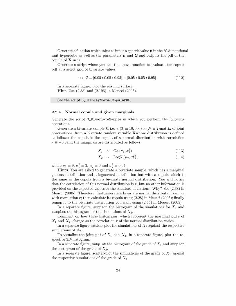
2.2.4 Normal copula and given marginals
Generate the script S_BivariateSample in which you perform the followingoperations.Generate a bivariate sample X, i.e. a (T ≡ 10, 000)× (N ≡ 2)matrix of joint
observations, from a bivariate random variable Xwhose distribution is definedas follows: the copula is the copula of a normal distribution with correlationr ≡ −0.8and the marginals are distributed as follows:
X1 ∼ Ga¡ν1, σ
21
¢(113)
X2 ∼ LogN¡µ2, σ
22
¢, (114)
where ν1 ≡ 9, σ21 ≡ 2, µ2 ≡ 0 and σ22 ≡ 0.04.Hints. You are asked to generate a bivariate sample, which has a marginal
gamma distribution and a lognormal distribution but with a copula which isthe same as the copula from a bivariate normal distribution. You will noticethat the correlation of this normal distribution is r, but no other information isprovided on the expected values or the standard deviations. Why? See (2.38) inMeucci (2005). Therefore, first generate a bivariate normal distribution samplewith correlation r; then calculate its copula using (2.28) in Meucci (2005); finallyremap it to the bivariate distribution you want using (2.34) in Meucci (2005).In a separate figure, subplot the histogram of the simulations for X1 and
subplot the histogram of the simulations of X2.Comment on how these histograms, which represent the marginal pdf’s of
X1 and X2, change as the correlation r of the normal distribution varies.In a separate figure, scatter-plot the simulations of X1 against the respective
simulations of X2.To visualize the joint pdf of X1 and X2, in a separate figure, plot the re-
spective 3D-histogram.In a separate figure, subplot the histogram of the grade of X1 and subplot
the histogram of the grade of X2.In a separate figure, scatter-plot the simulations of the grade of X1 against
the respective simulations of the grade of X2.
24
To visualize the joint pdf of the grades of X1 and X2, in a separate figureuse "hist3" to plot the respective 3D-histogram.
See the script S_BivariateSample.
2.2.5 FX copula-marginal factorization
Generate the script S_FXCopulaMarginalin which you perform the followingoperations.Load from db_FX the daily observations of the foreign exchange rates
USD/EUR, USD/GBP and USD/JPY. Define as variables the daily log-changesof the rates.Represent the marginal distribution of the three variables in simulation and
display the respective histogramsRepresent the copula of the three variables in simulation and display the
scatter-plot of the copula of all pairs of variables.Hint. Applying the marginal cdf to the simulations of a random variable is
equivalent to sorting
See the script S_FXCopulaMarginal.
2.2.6 Copula vs correlation
Consider a generic N -variate t random variable:
X ∼ St (ν,µ,Σ) . (115)
Generate the function TCopulaPDF which takes as input a generic value u inthe N -dimensional unit hypercube as well as the parameters ν, µ and Σ andoutputs the pdf of the copula of X in u.Hint. Use (2.30) and (2.188) in Meucci (2005) and the built-in functions
tpdf and tinv. Notice that you will have to re-scale the built-in pdf and thebuilt-in quantile of the standard t distribution.Generate a script where you call the above function to evaluate the copula
pdf at a select grid of bivariate values:
u ∈ G ≡ [0.05 : 0.05 : 0.95]× [0.05 : 0.05 : 0.95] . (116)
In a separate figure, plot the ensuing surface.Comment on the (dis)similarities with the normal copula when ν ≡ 200.Comment on the (dis)similarities with the normal copula when ν ≡ 1 and
Σ12 ≡ 0. What is the correlation in this case?
See the script S_DisplayCopulaPDF.From (2.191) in Meucci (2005), when the off-diagonal entries are null, the
marginals are uncorrelated, if the correlation is defined, which is true only for
25

ν > 2 (see fix in the Errata). Therefore, for ν > 2 null correlation does notimply independence, because the pdf is clearly not flat as ν → 2. For ν ≤ 2 thecorrelation simply does not exist. However the co-scatter parameter Σ12 can beset to zero, but this does not imply independence because, again, the pdf is farfrom flat as ν ≤ 2.
2.2.7 Full codependence
Generate J ≡ 10, 000 joint simulations for an N ≡ 10 -variate random variableX in such a way that each marginal is gamma-distributed
Xn ∼ Ga (n, 1) , n = 1, . . . , N , (117)
and such that each two entries are fully codependent, i.e. the cdf of their copulais (2.106).Hint. Use (2.34).
See the script S_FullCodependence.
3 Quest for invariance
3.1 Theory
3.1.1 Random walk
Generate a Merton jump-diffusion process Xt at discrete times with arbitraryparameters. What are the invariants in this process?Hint. This is a random walk
See the script S_DisplayJumpDiffusionMerton.The invariants are the non-overlapping changes in the process∆Xt over arbi-
trary intervals. Notice that these are not the only invariants, as any i.i.d. shockused to generate the process is also an invariant. However, these invariants aredirectly observable and their distribution can be estimated with the techniquesdiscussed in the course.
3.1.2 AR(1)
Generate an Ornstein-Uhlenbeck / AR(1) process.Prove empirically that for small time intervals and/or low reversion parame-
ters the Ornstein-Uhlenbeck process is a Brownian motion.Prove analytically that for small time intervals and/or low reversion para-
meters the Ornstein-Uhlenbeck process is a Brownian motion.
26
See the script S_AutocorrelatedProcess.Consider the solution of the Ornstein-Uhlenbeck process
XT+τ = m¡1− e−θτ
¢+ e−θτXT + T,τ , (118)
where
T,τ ∼ Nµ0,σ2
2θ
¡1− e−2θτ
¢¶. (119)
If θτ ≈ 0 we can write
XT+τ ≈ XT +mθτ + T,τ , (120)
whereT,τ ∼ N
¡0, σ2τ
¢, (121)
which is the standard arithmetic Brownian motion.
3.1.3 Volatility clustering
Generate a GARCH(1,1) process with arbitrary parameters. What are theinvariants of this process?
See the script S_VolatilityClustering.The invariants are the shocks in the volatility, which also directly drive
the randomness of the process. Notice that these invariants are not directlymeasurable.
3.2 Empirical
3.2.1 Equity
Consider any of the daily time series Pt of the stock prices in the databaseDB_Equities. Consider the variables
Xt ≡PtPt−1
(122)
Yt ≡ Pt − Pt−1 (123)
Zt ≡µ
PtPt−1
¶2(124)
Wt ≡ Pt+1 − 2Pt + Pt−1 (125)
Determine which among Xt, Yt, Zt, Wt, can potentially be an invariant andwhich certainly cannot be an invariant, by computing the histogram from twosub-samples and by plotting the location-dispersion ellipsoid of a variable withits lagged value.
27

See the script S_EquitiesInvariants. The Wt’s are clearly not invariants
3.2.2 Fixed income
Consider the time series of realizations of the yield curve in DB_FixedIncome.Check whether the changes in yield curve for a given time to maturity are
invariants using IIDAnalysis.Check whether the changes in the logarithm of the yield curve for a given
time to maturity are invariants using IIDAnalysis.
Changes in the yield curve and changes in the logarithm of the yield curveare approximately invariants, whereas the changes in the yield to maturity of aspecific bond are not, see the script S_FixedIncomeInvariants
3.2.3 Derivatives
Consider the time series of daily realizations of the implied volatility surface inDB_Derivatives.Check whether the weekly changes in implied volatility for a given level of
moneyness and time to maturity are invariants using IIDAnalysis.Check whether the weekly changes in the logarithm of the implied volatil-
ity for a given level of moneyness and time to maturity are invariants usingIIDAnalysis.Define the vector Zt as the juxtaposition of all the entries of the logarithm
of the implied volatility surface at time t. Fit the implied volatility data to amultivariate autoregressive process of order one:
Zt+1 ≡ ba+ bBZt + b²t+1, (126)
where time is measured in weeks. Check whether the weekly residuals b²t areinvariants using IIDAnalysis.
The weekly changes in (the logarithm of) the implied volatility are notinvariants, because they display significant negative autocorrelation. Onthe other hand, the weekly residuals b²t are invariants. See the scriptS_DerivativesInvariants
3.2.4 Cointegration
Upload the database DB_SwapParRates of the daily series of a set of par swaprates.Determine the (in-sample) decreasingly most cointegrated combination of
the above par swap rates using principal component analysis.Fit an AR(1) process to these combinations and compute the unconditional
(long term, equilibrium) expectation and standard deviation. Plot the 1-z-scorebands around the long-term mean to generate signals to enter or exit a trade.
28
Hint. See Meucci (2009b)
See the script S_StatArbSwaps.
4 Estimation
4.1 Non-parametric
4.1.1 Estimation of moment-based functional
Assume that the invariants Xt are distributed as a mixture. In other words, thepdf reads:
fX ≡ αfY + (1− α) fZ , (127)
where α ∈ (0, 1) and
fY ⇔ N¡µY , σ
2Y
¢(128)
fZ ⇔ LogN¡µZ , σ
2Z
¢. (129)
Consider the variable:
V ≡ αY + (1− α)Z, (130)
where Y and Z are independent and
Y ∼ N¡µY , σ
2Y
¢(131)
Z ∼ LogN¡µZ , σ
2Z
¢. (132)
Is (127) the pdf of (130)? If so, prove it. If not, how do you compute the pdf of(130)?
Formula (127) is not the pdf of (130). You can see this in simulation. Alter-natively, you can prove it by showing that the moments of X and the momentsof V are different. For instance, denote
s2Y ≡ E©Y 2ª, s2Z ≡ E
©Z2ª. (133)
Then
E©X2ª≡
Zu2fX (u) du (134)
= α
Zu2fY (u) du+ (1− α)
Zu2fZ (u) du
= αs2Y + (1− α) s2Z .
29
On the other hand
E©V 2ª≡ E
n(αY + (1− α)Z)2
o(135)
= Enα2Y 2 + 2α (1− α)Y Z + (1− α)2 Z2
o= α2 E
©Y 2ª+ 2α(1− α) E {Y }E {Z}+ (1− α)2 E
©Z2ª
= α2s2Y + (1− α)2s2Z .
Therefore (127) is not the pdf of (130). However, (127) is the pdf of a randomvariable, defined in distribution as follows:
Xd≡ BY + (1−B)Z. (136)
In this expression B is a Bernoulli variable:
B ∼ Ber (α) . (137)
This is a discrete random variable that can only assume two values:
B ≡½1 with probability α0 with probability 1− α
. (138)
Therefore, the pdf of B reads:
fB = αδ(1) + (1− α) δ(0), (139)
where δ(s) is the Dirac delta centered in s, see Figure B.2 in the textbook.When B = 1 in (136) the variable X will be normal as in (131), when B = 0
the variableX will be lognormal as in (132). Therefore, the pdf ofX conditionedon B reads:
fX|B (x|0) = fZ (x) , fX|B (x|1) = fY (x) . (140)
This two-step method gives rise to the pdf (127). To see this, as in (2.22) inMeucci (2005) the pdf of X can be written as the marginalization of the jointpdf of X and B:
fX (x) =
ZfX,B (x, b) db. (141)
As in (2.43) in Meucci (2005) the joint pdf of X and B can be written as theproduct of the conditional and the marginal:
fX,B (x, b) = fX|B (x|b) fB (b) . (142)
30
Therefore
fX (x) =
ZfX|B (x|b) fB (b) db (143)
=
ZfX|B (x|b)
hαδ(1) (b) + (1− α) δ(0) (b)
idb
= α
ZfX|B (x|b) δ(1) (b) db+ (1− α)
ZfX|B (x|b) δ(0) (b) db
= αfX|B (x|1) + (1− α) fX|B (x|0)= αfY (x) + (1− α) fZ (x) .
As for the pdf of (130), it can be obtained as follows.First we use (T1.14) in the technical appendices at symmys.com > Book >
Downloads with (1.67) and (1.95) in Meucci (2005) to compute the pdf of αYand (1− α)Z:
fαY (x) =1
αp2πσ2Y
exp
"−(x/α− µY )
2
2σ2Y
#(144)
f(1−α)Z (x) =1
xp2πσ2Z
exp
"−(ln (x/ (1− α))− µZ)
2
2σ2Z
#(145)
Then we compute the characteristic functions of αY and (1− α)Z as in (1.14)in Meucci (2005) as the Fourier transform of the respective pdf’s:
φαY = F [fαY ] , φ(1−α)Z = F£f(1−α)Z
¤. (146)
Then we compute the characteristic function of V :
φV (ω) ≡ E©eiωV
ª= E
neiω[αY+(1−α)Z]
o= E
©eiωαY
ªEneiω(1−α)Z
o(147)
= φαY (ω)φ(1−α)Z (ω)
= F [fαY ] (ω)F£f(1−α)Z
¤(ω) .
Using (B.45) in Meucci (2005) we can express the characteristic function of Vin terms of the convolution (B.43) of the pdf’s and the Fourier transform:
φV (ω) = F£fαY ∗ f(1−α)Z
¤(ω) . (148)
Then we compute the pdf of V as in (1.15) in Meucci (2005) as the inverseFourier transform of the characteristic function:
fV = F−1 [φV ] . (149)
31
Substituting (148) in (149) we finally obtain:
fV = F−1£F£fαY ∗ f(1−α)Z
¤¤(150)
= fαY ∗ f(1−α)Z .
Assume that we are interested in the following moment-based functional:
G [fX ] ≡ZR
¡x2 − x
¢fX (x) dx. (151)
Compute (151) analytically as a function of the inputs α, µY , σY , µZ and σZ .
G [fX ] ≡ZR
¡x2 − x
¢fX (x) dx (152)
= α
ZR
¡x2 − x
¢fY (x) dx+ (1− α)
ZR
¡x2 − x
¢fZ (x) dx
= α³Var {Y }+ (E {Y })2 − E {Y }
´+(1− α)
³Var {Z}+ (E {Z})2 − E {Z}
´(1.71)(1.72)(1.98)(1.99)
= α¡µ2Y + σ2Y − µY
¢+(1− α)
µe2µZ+2σ
2Z − eµZ+
σ2Z2
Build a function QuantileMixture that computes the quantile of (127) bylinear interpolation/extrapolation of the respective cdf on a fine set of equallyspaced points for generic values of α, µY , σY , µZ , σZ . In order to use this func-tion in the sequel, make sure the function can accept a vector of values u in(0, 1) as input, not just one value, thereby outputting the respective vector ofvalues x ≡ QX (u) in the domain of X.Hint. Use the built-in cumulative distribution functions that correspond to
(128) and (129).Assume knowledge of the following parameters:
α ≡ 0.8, σY ≡ 0.2, µZ ≡ 0, σZ ≡ 0.15. (153)
Set µY ≡ 0.1 and generate a sample of T ≡ 52 i.i.d. observations
iT ≡ {x1, . . . , xT } (154)
from the distribution (127).Hint. feed a uniform sample into the function QuantileMixture.
32
See the script S_GenerateMixtureSample.
Consider the following estimators:bGa [iT ] ≡ (x1 − xT )x22 (155)
bGb [iT ] ≡1
T
TXt=1
xt (156)
bGc [iT ] ≡ 5. (157)
Evaluate the performance of the estimators (155), (156) and (157) with respectto (151) as in the script S_Estimator by assuming (153) and by stress-testingthe parameter µY in the range [0, 0.2].
See script S_EstimateMomentsComboEvaluation.
Compute the non-parametric estimator bGd of (151) defined by (4.36). As-sume knowledge of the parameters (153) and evaluate the performance of bGd
with respect to (151) as in the script S_EstimateExpectedValueEvaluationby stress-testing the parameter µY in the range [0, 0.2].
See script S_EstimateMomentsComboEvaluation.The non-parametric estimator of
G [fX ] ≡ZR
¡x2 − x
¢fX (x) dx (158)
follows from (4.36) in Meucci (2005):
bGd (iT ) ≡ZR
¡x2 − x
¢fiT (x) dx (159)
=
ZRx2fiT (x) dx−
ZRxfiT (x) dx.
The second term is the sample mean (1.126) in Meucci (2005):
bm ≡ ZRxfiT (x) dx =
1
T
TXt=1
xt (160)
The first term is the sample non-central second moment:
cns ≡ ZRx2fiT (x) dx =
1
T
TXt=1
x2t . (161)
By applying (T1.39) in the technical appendices at symmys.com > Book >Download to (1.126) and (1.127) in Meucci (2005) we obtain
cns = bs2 + bm2, (162)
33
where bs2 is the sample variance (1.127) in Meucci (2005):bs2 ≡ 1
T
TXt=1
(xt − bm)2 . (163)
Therefore
bGd (iT ) = cns− bm (164)
= bs2 + bm2 − bm.4.1.2 Estimation of quantile
Assume that we are interested in this functional:
G [fX ] ≡ (I [fX ])−1 (p) , (165)
where I [·] is the integration operator and p ≡ 0.5. Notice that the above issimply the quantile with confidence p, see (1.8) and (1.17) in Meucci (2005):
G [fX ] ≡ QX (p) . (166)
In particular, given that p ≡ 0.5, the above is the median.Compute the non-parametric estimator bqp of (165) defined by (4.36) in
Meucci (2005). Assume knowledge of the parameters (153) and evaluate theperformance of bqp with respect to (165) as in the script S_Estimator by stress-testing the parameter µY in the range [0, 0.2].Hint. Use the function QuantileMixture.
See script S_EstimateQuantileEvaluation.From (4.39) in Meucci (2005), the non-parametric estimator of the median
is the sample median (1.130) in Meucci (2005):
bGe (iT ) ≡ x[T/2]:T . (167)
Evaluate the performance of the estimator (156) with respect to (165) as inthe script S_Estimator by stress-testing the parameter µY in the range [0, 0.2].Hint. Use the function QuantileMixture.
See script S_EstimateQuantileEvaluation.
4.2 Maximum likelihood
4.2.1 Basics
Consider the time series of realizations of the random variable X in the databaseDBTimeSeries.
34
Check that the provided series represents the realizations of an invariantusing IIDAnalysis.Assuming that X is an invariant, let fX denote the unknown pdf that rep-
resents the unknown distribution of each realization in the time series. Makethe following assumption on the generating process for X, where we use thenotation of (1.79) and (1.95) in Meucci (2005):
fX ≈ fθ ≡(
fCaθ,θ2
for θ ∈ [−0.04,−0.01]fLogNθ,(θ−0.01)2 for θ ∈ ({0.02} ∪ {0.03}) (168)
Compute numerically the maximum likelihood estimator bθML of θ.Hint. Approximate the continuum [−0.04,−0.01] with a fine set of equally
spaced points; evaluate the (log-)likelihood for every value of θ.Assume now that you are interested in the p-quantile of X for p ≡ 1%, as
defined in (1.17). Use the above result to compute the ML estimator bqMLp and
compare this ML estimate with the non-parametric estimate of the quantile forthe same confidence level.Hint. As in (4.38) in Meucci (2005), the true quantile is a functional of the
unknown distribution of X:
Qp (X) ≡ qp [fX ] . (169)
Therefore, the ML estimator of the quantile is the functional applied to theML-estimated distribution:
bqMLp ≡ qp
hfθML
i. (170)
On the other hand, as in (4.36) in Meucci (2005) the non-parametric quantileis the functional applied to the empirical pdf:
bqNPp ≡ qp [fiT ] , (171)
see also Section 4.2.1.
See script S_MLEbasics.
4.2.2 MLE for univariate elliptical variables
Consider as in (1.28) in Meucci (2005) a symmetrical univariate random vari-able X. It is easy to check that such distributions are all and only the one-dimensional elliptical distributions. In other words, there exist two numbers µand σ and a univariate function g such that:
X ∼ El¡µ, σ2, g
¢. (172)
Assume that you know the functional form of g. Adapt the proof in the tech-nical appendix www.4.2 at symmys.com > Book > Downloads to compute themaximum likelihood estimators bµ and bσ2 of µ and σ2 respectively.
35
First of all we need two general results. Define
M2t ≡ ω2 (xt − µ)
2 , (173)
Then
∂M2t
∂µ= −2ω2 (xt − µ) (174)
∂M2t
∂ω2= (xt − µ)
2 (175)
Now assume that the distribution of the invariants is (172). To compute the MLestimators bµ and bσ2 we have to maximize the likelihood function as in (4.66) inMeucci (2005), which after (4.74) reads:³bµ [iT ] , bσ2 [iT ]´ ≡ argmax
µ,σ2∈Θ
TXt=1
ln
Ã1√σ2
g
Ã(xt − µ)
2
σ2
!!, (176)
where the parameter set isΘ ≡ R×R+. (177)
We neglect the constraint that σ2 be positive and verify ex-post that the un-constrained solution satisfies this condition. It is easier to compute the MLestimators of µ and ω2 ≡ 1/σ2. The ML estimator of σ2 is simply the inverseof the estimator of ω2 by the invariance property (4.70) in Meucci (2005) of theML estimators.The log-likelihood reads:
ln (fθ (iT )) =T
2ln¯̄ω2¯̄+
TXt=1
ln£g¡M2
t
¢¤. (178)
The first order conditions with respect to µ read:
0 =∂
∂µ[ln (fθ (iT ))] (179)
=∂
∂µ
"TXt=1
ln fθ (xt)
#
=∂
∂µ
"TXt=1
ln£g¡M2
t
¢¤#
=TXt=1
g0¡M2
t
¢g (M2
t )
∂M2t
∂µ=
TXt=1
wtω2 (xt − µ) ,
where we used (174) and we defined:
wt ≡ −2g0¡M2
t
¢g (M2
t ). (180)
36
The solution to this equations is
bµ = PTt=1wtxtPTs=1ws
. (181)
The first order conditions with respect to ω2 read
0 =∂ ln (fθ (iT ))
∂ω2=
∂PT
t=1 ln fθ (xt)
∂ω2(182)
=T
2
∂ ln¡ω2¢
∂ω2+
TXt=1
g0¡M2
t
¢g (M2
t )
∂M2t
∂ω2
=T
2
1
ω2− 12
TXt=1
wt (xt − µ)2 ,
where in the last row we used (175).Thus the solution to (182) reads:
bσ2 ≡ 1³cω2´ = 1
T
TXt=1
wt (xt − bµ)2 (183)
This number is positive and thus the unconstrained optimization is correct.
4.2.3 MLE for multivariate Student t distribution
Consider t-distributed invariants:
X ∼ St (ν,µ,Σ) . (184)
Assume ν known and use (4.80)-(4.82) in Meucci (2005) to build a recursiveroutine that computes the ML estimates bµML and bΣML of µ andΣ respectively.Hint. The "pen & paper" part will lead you to the weights (4.80) in Meucci
(2005) . First compute the generator g that appears in the weighting function(4.79) in Meucci (2005). Under the Student t assumption the pdf is (2.188) inMeucci (2005) and the generator follows accordingly. Now you can compute theweighting function (4.79) in Meucci (2005), namely:
w (z) ≡ −2g0 (z)
g (z). (185)
Finally, you can compute the weights (4.80) in Meucci (2005) in MATLAB.Upload the database DBUsSwapRates of the daily time series of par 2yr,
5yr and 10yr swap rates. Compute the invariants relative to a daily estimationinterval. Then use the above routine to estimate the expectation and the covari-ance relative to the 2yr and the 5yr rates under the assumption that ν ≡ 3 and
37
ν ≡ 100 respectively. Represent the two sets of expectations and the covariancesin one figure in terms of the ellipsoid. Also scatter-plot the observations.
See script S_FitSwapToT.First we have to compute the generator g that appears in the weighting
function (4.79). Under the Student t assumption the pdf is (2.188). Thus, as in(2.188) the generator reads:
g (z) ≡Γ¡ν+N2
¢Γ¡ν2
¢(νπ)
N2
³1 +
z
ν
´− ν+N2
. (186)
Hence the weighting function (4.79) reads:
w (z) ≡ −2g0 (z)
g (z)=
ν +N
ν + z. (187)
Therefore the weights (4.80) read:
wt ≡ν +N
ν + (xt − bµ)0 bΣ−1 (x− bµ) . (188)
4.3 Shrinkage
4.3.1 Location
Fix N ≡ 5 and generate a N -dimensional location vector µ and a N×N scattermatrix Σ.Consider a normal random variable:
X ∼ N(µ,Σ) . (189)
Generate a time series of T ≡ 30 observations from (189).Build a function that computes the shrinkage estimator (4.138) in Meucci
(2005).
See script S_ShrinkageEstimators.
4.3.2 Scatter
Build a function that computes the shrinkage estimator (4.160) in Meucci (2005).
See script S_ShrinkageEstimators.
38
4.3.3 Sample covariance and eigenvalue dispersion
Fix N ≡ 50, µ ≡ 0N , Σ ≡ IN . Reproduce the surface in Figure 4.15. You donot need to superimpose the true spectrum as in the figureHints: Determine a grid of values for the number of observations T in the
time series. For each value of Ta) generate an i.i.d. time series
iT ≡ {x1, . . . ,xT } (190)
fromX ∼ N(µ,Σ) . (191)
b) compute the sample covariance bΣ.c) perform the PC decomposition of bΣ and store the sample eigenvalues (i.e.the sample spectrum)d) perform a)-c) a large enough number of times (~ 100 times)e) compute the average sample spectrum
See script S_EigenvalueDispersion.
4.4 Random matrix theory
4.4.1 Semi-circular law
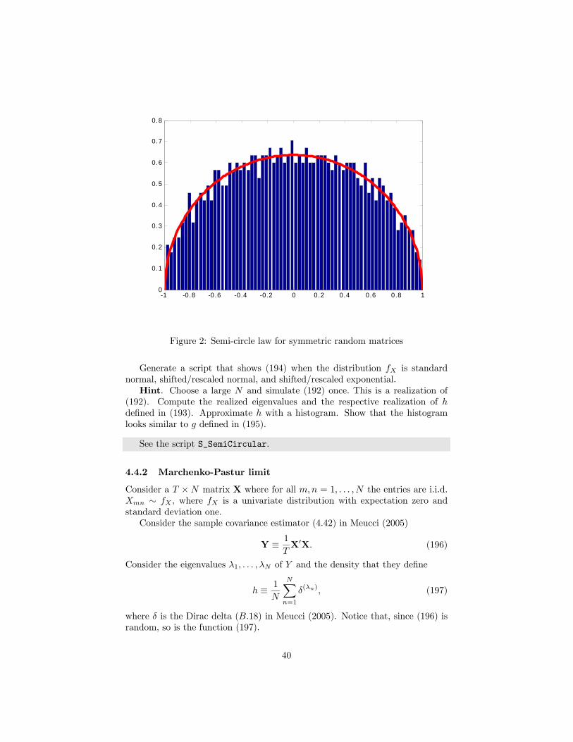
Consider a N ×N matrix X where for all m,n = 1, . . . , N the entries are i.i.d.Xmn ∼ fX , where fX is a univariate distribution with expectation zero andstandard deviation one.Consider the symmetrized and rescaled matrix
Y ≡ 1√8N
(X+X0) . (192)
Consider the eigenvalues λ1, . . . , λN of Y and the density that they define
h ≡ 1
N
NXn=1
δ(λn), (193)
where δ is the Dirac delta (B.18) in Meucci (2005). Notice that, since (192) israndom, so is the function (193).According to random matrix theory, in some topology the following limit for
the random function h holdslim
N→∞h = g, (194)
where g is the rescaled upper semicircle function, defined for λ ≥ 0 as follows
g (λ) ≡ 2
π
p1− λ2. (195)
39
-1 -0.8 -0.6 -0.4 -0.2 0 0.2 0.4 0.6 0.8 10
0.1
0.2
0.3
0.4
0.5
0.6
0.7
0.8
Figure 2: Semi-circle law for symmetric random matrices
Generate a script that shows (194) when the distribution fX is standardnormal, shifted/rescaled normal, and shifted/rescaled exponential.Hint. Choose a large N and simulate (192) once. This is a realization of
(192). Compute the realized eigenvalues and the respective realization of hdefined in (193). Approximate h with a histogram. Show that the histogramlooks similar to g defined in (195).
See the script S_SemiCircular.
4.4.2 Marchenko-Pastur limit
Consider a T ×N matrix X where for all m,n = 1, . . . , N the entries are i.i.d.Xmn ∼ fX , where fX is a univariate distribution with expectation zero andstandard deviation one.Consider the sample covariance estimator (4.42) in Meucci (2005)
Y ≡ 1
TX0X. (196)
Consider the eigenvalues λ1, . . . , λN of Y and the density that they define
h ≡ 1
N
NXn=1
δ(λn), (197)
where δ is the Dirac delta (B.18) in Meucci (2005). Notice that, since (196) israndom, so is the function (197).
40
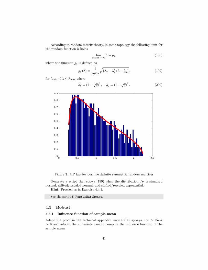
According to random matrix theory, in some topology the following limit forthe random function h holds
limN≡qT→∞
h = gq, (198)
where the function gq is defined as
gq (λ) ≡1
2qπλ
q¡λq − λ
¢ ¡λ− λq
¢, (199)
for λmin ≤ λ ≤ λmax where
λq ≡ (1−√q)2, λq ≡ (1 +
√q)2 . (200)
0 0.5 1 1.5 2 2.50
0.1
0.2
0.3
0.4
0.5
0.6
0.7
0.8
0.9
Figure 3: MP law for positive definite symmetric random matrices
Generate a script that shows (199) when the distribution fX is standardnormal, shifted/rescaled normal, and shifted/rescaled exponential.Hint. Proceed as in Exercise 4.4.1.
See the script S_PasturMarchenko.
4.5 Robust
4.5.1 Influence function of sample mean
Adapt the proof in the technical appendix www.4.7 at symmys.com > Book> Downloads to the univariate case to compute the influence function of thesample mean.
41
Sample estimators of the unknown quantity G [fX ] are by definition explicitfunctionals of the empirical pdf:
eG [fiT ] ≡ G [fiT ] . (201)
Therefore from its definition (4.185) in Meucci (2005) the influence functionreads:
IF³y, fX , bG´ ≡ lim→0 1 ³G h(1− ) fX + δ(y)
i−G [fX ]
´, (202)
where y is an arbitrary point. Now consider the function:
h ≡ (1− ) fX + δ(y). (203)
The influence function can be written:
IF³y, fX , bG´ ≡ lim→0 1 (G [h ]−G [h0]) =
dG [h ]
d
¯̄̄̄0
. (204)
Consider the functional associated with the sample mean bµ, which reads:eµ [h] ≡ Z
Rxh (x) dx. (205)
From (204) the influence function reads:
IF (y, f, bµ) ≡ deµ [h ]d
¯̄̄̄0
. (206)
First we compute:
eµ [h ] ≡ ZRxh (x) dx (207)
=
ZRx³(1− ) f (x) + δ(y) (x)
´dx
= (1− )
ZRxf (x) dx+ y
= E {X}+ (−E {X}+ y) .
From this and (206) we derive:
IF (y, f, bµ) = −E {X}+ y. (208)
4.5.2 Influence function of sample variance
Adapt the proof in the technical appendix www.4.7 at symmys.com > Book> Downloads to the univariate case to compute the influence function of the
42
sample variance.
Consider the functional associated with the sample variance bσ2, which reads:eσ2 [h] ≡ Z
R(x− eµ [h])2 h (x) dx. (209)
From (204) the influence function reads:
IF³y, f, bσ2´ ≡ lim
→0
1 ³eσ2 [h ]− eσ2 [h0]´ = deσ2 [h ]d
¯̄̄̄¯0
. (210)
First we compute:
eσ2 [h ] ≡ ZR(x− eµ [h ])2 h (x) dx (211)
=
ZR(x− eµ [h ])2 ³(1− ) f (x) + δ(y) (x)
´dx
= (1− )
ZR(x− eµ [h ])2 f (x) dx+ (y − eµ [h ])2
Deriving this expression with respect to we obtain:
IF³y, f, bσ2´ =
deσ2 [h ]d
¯̄̄̄¯0
(212)
= −ZR(x− eµ [h0])2 f (x) dx
+(1− 0)ZR
d
d
¯̄̄̄0
(x− eµ [h ])2 f (x) dx+(y − eµ [h0])2+0× d
d
¯̄̄̄0
(y − eµ [h ])2Using eµ [h0] = E {X} this means:
IF³y, f, bσ2´ = −Var {X} (213)
−ZR2deµ [h ]d
¯̄̄̄0
(x− E {X}) f (x) dx
+(y − E {X})2
Now using (208) we obtain:
IF³y, f, bσ2´ = −Var {X} (214)
−2ZR(y − E {X}) (x− E {X}) f (x) dx
+(y − E {X})2
43
The term in the middle is null. Therefore:
IF³y, f, bσ2´ = −Var {X}+ (y − E {X})2 (215)
4.6 Bayesian
4.6.1 Prior on correlation
Assume that the returns Xt ≡ (Xt,1,Xt,2,Xt,3)0 on three stocks are jointly
normal:Xt ∼ N(µ,Σ) , (216)
with null expectations and unit standard deviations:
µ ≡
⎛⎝ 000
⎞⎠ (217)
Σ ≡
⎛⎝ 1 θ12 θ13θ12 1 θ23θ13 θ23 1
⎞⎠ (218)
In this situation the joint distribution of the returns is fully determined by threeparameters:
θ ≡ (θ12, θ13, θ23)0 . (219)
These parameters are constrained on a domain:
θ ∈ Θ ⊂ (−1, 1)× (−1, 1)× (−1, 1) . (220)
Since Σ must be positive definite, the domain Θ is a proper subset of (−1, 1)×(−1, 1)× (−1, 1). For instance, θ ≡ − (.9, .9, .9)0 is not a feasible value.Assume an uninformative uniform prior for the correlations. In other words,
assume that θ is uniformly distributed on its domain:
θ ∼ U(Θ) . (221)
Generate 10, 000 simulations from (221).Hint. Generate a uniform distribution on (−1, 1)3 then discard the simula-
tions such that Σ is not positive definite.In three subplots plot the histograms of θ12, θ13 and θ23 respectively, showing
how the uniform prior implied non-uniform marginal distributions on each ofthe correlations.
See the script S_CorrelationPriorUniform.
44
4.6.2 Normal-Inverse-Wishart posterior
Create a function randNIW that takes as inputs a generic N -dimensional vectorµ0, a generic positive and symmetric N ×N matrix Σ0, two positive scalars T0and ν0 and the number of simulations J and outputs J independent simulationsof the normal-inverse-Wishart distribution, as defined in (7.20)-(7.21) in Meucci(2005).In a script S_AnalyzeNIWPriorPosterior upload the database DBUsSwapRates
of daily USD swap rates and compute the daily rate changes from. Then com-pute T , bµ and bΣ (see Chapter 7 for the notation).In the same script S_AnalyzeNIWPriorPosterior set ν0 ≡ T0 ≡ 52 and
define the prior parameters µ0 and Σ0 arbitrarily. Use the function randNIW togenerate J ≡ 104 scenarios of the prior (7.20)-(7.21) in Meucci (2005).In the same script S_AnalyzeNIWPriorPosterior compute the parameters
of the posterior distribution and use the function randNIW to generate J ≡ 104scenarios of the posterior.Specialize the script S_AnalyzeNIWPriorPosterior to the case N ≡ 1, i.e.
only consider the first swap rate change.In one figure, subplot the histogram of the marginal distribution of the prior ofµ and superimpose the profile of its analytical pdf. Then subplot the histogramof the marginal distribution of the prior of 1/σ2 and superimpose the profile ofits analytical pdf.In a different figure, subplot the histogram of the marginal distribution of theposterior of µ and superimpose the profile of its analytical pdf. Then subplot thehistogram of the marginal distribution of the posterior of 1/σ2 and superimposethe profile of its analytical pdf.Check that (7.4) in Meucci (2005) holds by changing the relative weights ofν0, T0 with respect to T .
See script S_AnalyzeNIWPriorPosterior.
4.7 Missing data
4.7.1 EM algorithm
Consider the attached database db_HighYieldIndices of the daily time seriesof high-yield bond indices. As you will see, some observations are missing.Compute the time series of the daily compounded returns, replacing "NaN" forthe missing observations.Assume that the distribution of the daily compounded returns is normal
Xt ∼ N(µ,Σ) . (222)
Estimate the parameters (µ,Σ) by means of the EM algorithm2.
2Check the online Errata at symmys.com > Book > Downloads, as there is a typo in thefirst and second printing of the textbook (no typo from the third printing).
45
See script S_EMexampleHighYield.
4.8 Testing
4.8.1 Sample mean
Consider a time series of independent and identically distributed random vari-ables
Xt ∼ N¡µ, σ2
¢, t = 1, . . . , T . (223)
Consider the sample mean
bµ ≡ 1
T
TXt=1
Xt. (224)
Compute the distribution of bµ.We can write⎛⎜⎝ X1
...XT
⎞⎟⎠ ∼ N⎛⎜⎜⎝⎛⎜⎝ µ
...µ
⎞⎟⎠ ,
⎛⎜⎜⎝σ2 0 · · ·
0. . .
... σ2
⎞⎟⎟⎠⎞⎟⎟⎠ . (225)
From (2.163) in Meucci (2005), which we report here
X ∼ N(µ,Σ)⇒ a+BX ∼ N¡a+Bµ,BΣB0
¢for any conformable vector and matrix a and B respectively, it follows
bµ ∼ Nµµ, σ2T
¶. (226)
What is the probability that the sample mean (224) exceed a given value eµ?P {bµ > eµ} = 1− P {bµ ≤ eµ} (227)
= 1− P( bµ− µp
σ2/T≤ eµ− µp
σ2/T
)From (4.8.1) and (226) it followsbµ− µp
σ2/T∼ N(0, 1) , (228)
therefore
P {bµ > eµ} = 1− ΦÃ eµ− µpσ2/T
!, (229)
46
where Φ denotes the cdf of the standard normal distribution.
4.8.2 p-value analytical
Consider a normal invariant
Xt ∼ N¡µ, σ2
¢(230)
in a time series of length T . Consider the ML estimator bµ of the locationparameter µ. Suppose that you observe a value eµ for the estimator. Assumethat you believe that
µ ≡ µ0, σ2 ≡ σ20. (231)
The p-value of bµ for eµ under the hypothesis (231) is the probability ofobserving a value as extreme as the observed value:
p ≡ P {bµ ≶ eµ} . (232)
Compute the expression of the p-value in terms of the cdf of the estimator.
From (4.102) in Meucci (2005)
bµ ∼ Nµµ, σ2T
¶. (233)
Therefore in the notation of (1.68) in Meucci (2005) we obtain
p ≡ P {bµ ≤ eµ} = FNµ0,σ
20/T
(eµ) (234)
or
p ≡ P {bµ ≥ eµ} = 1− P {bµ ≤ eµ} (235)
= 1− FNµ0,σ
20/T
(eµ) .4.8.3 t-test, location, analytical
Consider a normal invariant
Xt ∼ N¡µ, σ2
¢(236)
in a time series of length T . Consider the ML estimators bµ and bσ2 of the locationand scatter parameters µ and σ2 respectively. The t-statistic for bµ is defined as
btµ0 ≡ bµ− µ0qbσ2/ (T − 1) . (237)
Compute the distribution of btµ.47
Hint. Recall that if Yσ2 and Zν are independent and such that
Yσ2 ∼ N¡0, σ2
¢(238)
νZ2ν ∼ χ2ν (239)
then
Xν,σ2 ≡Yσ2pZ2ν∼ St
¡ν, 0, σ2
¢. (240)
From (4.103), (1.106) and (1.109) in Meucci (2005) it follows
(T − 1)Ã
T
T − 1bσ2σ2
!∼ χ2T−1. (241)
From (233) we obtain rT
σ2(bµ− µ) ∼ N(0, 1) . (242)
Furthermore, from the proof in Appendix www.4.3 we derive that bµ and bσ2 areindependent. From (240), we obtain
btµ ≡ bµ− µqbσ2/ (T − 1) (243)
=
rT
σ2(bµ− µ)
1qTσ2
(T−1)σ2
d=
Y1qZ2T−1
.
Therefore btµ ∼ St (T − 1, 0, 1) . (244)
You would like to ascertain whether it is possible that
µ = µ0 (245)
for an arbitrary value µ0 in (236). How can you asses if the hypothesis (245) isacceptable?
First, compute the distribution of (237) under (245). Then compute therealization etµ0 of (237). In the notation (1.87) in Meucci (2005) we obtain:
P©btµ0 ≤ etµ0ª = F StT−1,0,1
¡etµ0¢ (246)
P©btµ0 ≥ etµ0ª = 1− F StT−1,0,1
¡etµ0¢ . (247)
Therefore, if tα is so small or so large that either probabilities are too small,then (245) is very unlikely.
48

4.8.4 t-test, factor loadings, analytical
Consider two jointly normal invariantsµXt
Ft
¶∼ N
µµµXµF
¶,
µσ2X ρσXσF
ρσXσF σ2F
¶¶. (248)
Consider a conditional model of the kind (4.88) in Meucci (2005):
Xt = α+ βft + Ut, (249)
whereUt|ft ∼ N
¡0, σ2
¢. (250)
What is the conditional model (249)-(250) ensuing from (248)?
See (2.173) and/or (3.130)-(3.131) in Meucci (2005) to derive
α ≡ µX − ρσXσF
µF (251)
β ≡ ρσXσF
(252)
σ2 ≡ σ2X¡1− ρ2
¢. (253)
Consider the conditional model (249)-(250) for the invariants. Compute the
ML estimators of the factor loadings³bα, bβ´ given the observations
iT ≡ {x1, f1, . . . , xT , fT } . (254)
Hint. Define f 0t ≡ (1, ft) and
bΣXF ≡ 1
T
TXt=1
xtf0t (255)
bΣF ≡ 1
T
TXt=1
ftf0t . (256)
Follow the proof of (4.126) in Meucci (2005) to derive³bα, bβ´ = bΣXFbΣ−1F , (257)
Compute the joint distribution of the ML estimators of the factor loadings³bα, bβ´ under the conditional model (249)-(250).
49
Follow the proof of (4.129) in Meucci (2005) to derive in terms of a (degen-erate) matrix-valued normal distribution³bα, bβ´ ∼ Nµ(α, β) , σ2
T, bΣ−1F 
. (258)
From (2.180) in Meucci (2005) we then obtainµ bαbβ¶∼ N
µµαβ
¶,σ2
TbΣ−1F 
. (259)
Compute the distribution of the ML estimator bσ2 of the dispersion parameterthat appears in (250).
Follow the proof of (4.130) and use (2.230) in Meucci (2005) to derive
Tbσ2 ∼ Ga ¡T − 2, σ2¢ . (260)
Compute the distribution of the t-statistic for bαbtα ≡ √T − 2(bα− α)qbσ2bσ2α (261)
and the distribution of the t-statistic for bβbtβ ≡ √T − 2 bβ − βqbσ2bσ2β , (262)
where bσ2α is the north-west entry of bΣ−1F and bσ2β is its south-east entry.From (260), (1.106) and (1.109) in Meucci (2005) it follows
(T − 2)Ã
T
T − 2bσ2σ2
!∼ χ2T−2. (263)
From (259) we obtain sTbσ2ασ2 (bα− α) ∼ N(0, 1) , (264)
and similarly for β. Furthermore, follow the proof in Appendix www.4.4 to
50
derive that³bα, bβ´ and bσ2 are independent. Using (240), we obtain
btα ≡√T − 2(bα− α)qbσ2bσ2α (265)
=
qT
σ2ασ2 (bα− α)qT
T−2σ2
σ2
Then from (240) we derive
btα d=
Y1qZ2T−2
∼ St (T − 2, 0, 1) , (266)
You would like to ascertain whether it is possible that
α = α0 (267)
for an arbitrary value α0 in (249), typically α0 ≡ 0. How can you asses if thehypothesis (267) is acceptable?
First, compute the distribution of (261) under (267). Then compute therealization etα0 of (261). In the notation (1.87) in Meucci (2005) we obtain:
P©btα0 ≤ etα0ª = F Stν,0,1
¡etα0¢ (268)
P©btα0 ≥ etα0ª = 1− F Stν,0,1
¡etα0¢ . (269)
Therefore, if tα is so small or so large that either probabilities are too small,then (267) is very unlikely.
More in general, consider a conditional model of the kind (4.88) in Meucci(2005)
Xt|ft = b0ft + Ut, (270)
where ft is a set of K factors that include a constant and
Ut|ft ∼ N¡0, σ2
¢. (271)
Consider the ML estimator bb of b. Compute the distribution of the F -statisticfor the linear assumptions A
bFb ≡ (T − 2)³bb− b´0A0A
³bb− b´bσ2 (272)
and use this result to asses if a hypothesis
Ab = a (273)
is acceptable for arbitrary conformable matrix/vector pairs A and a.
51
4.8.5 Generalized t-tests, simulations
Consider a joint model for the invariants: for t = 1, . . . , T . The marginals are
Xt ∼ LogN¡µX , σ
2X
¢, (274)
Ft ∼ Ga¡νF , σ
2F
¢; (275)
and the copula is the copula of the diagonal entries of Wishart distribution
Wt ∼W(νW ,ΣW ) . (276)
Consider the coefficients that define the regression line (3.127)
eXt ≡ α+ βFt. (277)
Compute the non-parametric estimators³bα, bβ´ of the regression coefficients.
From (4.52) in Meucci (2005) they read as in (257).
Are³bα, bβ´ the maximum-likelihood estimators of the regression coefficients?
No, because the regression model ensuing from (274)-(276) is not condition-ally normal as in (249)-(250).
Generate arbitrary values for the parameters in (274)-(276) and for the num-ber of observations T and compute in simulation the distribution of the statistic
bGα ≡√T − 2(bα− α)qbσ2bσ2α (278)
and the distribution of the statistic
bGβ ≡√T − 2
bβ − βqbσ2bσ2β . (279)
Compare the empirical distribution of (278) with the analytical distribu-tion of (261) as well as the empirical distribution of (279) with the analyticaldistribution of (262) and comment.
See script S_TStatApprox. The distribution of (278) is very similar to thatof (261) even for relatively small values of T . The same holds for the distributionof (279) as compared to that of (262).
52
5 Projection and pricing
5.1 Projection of skewness, kurtosis, and all standardizedsummary statistics
This exercise is discussed in greater depth and placed into a broader context inMeucci (2010a), freely available online at ssrn.com.Consider an invariant, which we denote by Xt, refer to the "quest for invari-
ance" in Meucci (2005), Meucci (2009a) and Meucci (2010c). Assume that wehave properly estimated the distribution of such one-period invariant. Then wecan compute the expectation (1.25) in Meucci (2005)
µX ≡ E{X}; (280)
the standard deviation (1.42) in Meucci (2005)
σX ≡pE{(X − µX)
2}; (281)
the skewness (1.49) in Meucci (2005)
skX ≡ E{(X − µX)3}/σ3X ; (282)
the kurtosis (1.51) in Meucci (2005)
kuX ≡ E{(X − µX)4}/σ4X ; (283)
and in general n-th standardized summary statistics
γ(n)X ≡ E{(X − µX)
n}/σnX , n ≥ 3. (284)
Consider the projected invariant, defined as the sum of k intermediate single-period invariants
Y = X1 + · · ·+Xk. (285)
Such rule applies e.g. to the compounded return (3.11) in Meucci (2005), butnot to the linear return (3.10) in Meucci (2005), see also Meucci (2005) for thispitfall.Project the single-period statistics (280)-(284) to the arbitrary horizon k, i.e.
compute the first n standardized summary statistics for the projected invariantY
µY , σY , skY , kuY , γ(5)Y , . . . , γ
(n)Y (286)
from the first n single-period statistics for the single-period invariant X
µX , σX , skX , kuX , γ(5)X , . . . , γ
(n)X . (287)
Hints.Use the central moments, see (1.48) in Meucci (2005)
µ(1)X ≡ µX ; µ
(n)X ≡ E{(X − µX)
n}, n = 2, 3, . . . ; (288)
53
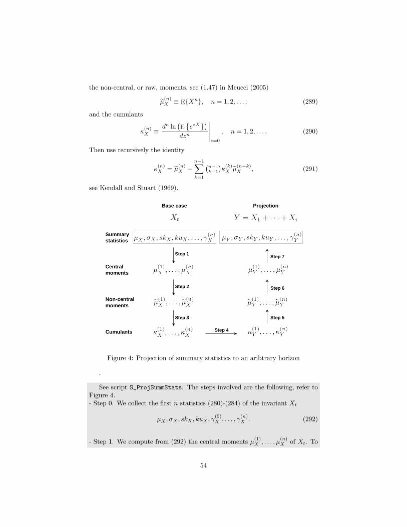
the non-central, or raw, moments, see (1.47) in Meucci (2005)
eµ(n)X ≡ E{Xn}, n = 1, 2, . . . ; (289)
and the cumulants
κ(n)X ≡
dn ln¡E©ezX
ª¢dzn
¯̄̄̄¯z=0
, n = 1, 2, . . . . (290)
Then use recursively the identity
κ(n)X = eµ(n)X −
n−1Xk=1
¡n−1k−1¢κ(k)X eµ(n−k)X , (291)
see Kendall and Stuart (1969).
Base case Projection
Summary statistics
Central moments
Non-central moments
Cumulants
Step 1
Step 2
Step 3
Step 4
Step 5
Step 6
Step 7
Figure 4: Projection of summary statistics to an aribtrary horizon
.
See script S_ProjSummStats. The steps involved are the following, refer toFigure 4.- Step 0. We collect the first n statistics (280)-(284) of the invariant Xt
µX , σX , skX , kuX , γ(5)X , . . . , γ
(n)X . (292)
- Step 1. We compute from (292) the central moments µ(1)X , . . . , µ(n)X of Xt. To
54

do so, notice from the definition of central moments (288) that µ(2)X ≡ σ2X andthat from (284) we obtain
µ(n)X = γ
(n)X σnX , n ≥ 3. (293)
- Step 2. We compute from the central moments µ(1)X , . . . , µ(n)X the non-central
moments eµ(1)X , . . . , eµ(n)X of Xt, see Exercise 1.1.8.- Step 3. We compute from the non-central moments eµ(1)X , . . . , eµ(n)X the cumu-lants κ(1)X , . . . , κ
(n)X of Xt. To do so, we start from κ
(1)X = eµ(1)X : this follows from
the Taylor approximations E©ezX
ª≈ E {1 + zX} = 1 + zeµ(1)X for any small z
and ln(1 + x) ≈ x for any small x, and from the definition of the first cumulantin (290). Then we apply recursively the identity (291).- Step 4. We compute from the cumulants κ
(1)X , . . . , κ
(n)X of Xt the cumu-
lants κ(1)Y , . . . , κ(n)Y of the projection Y ≡ X1 + · · · + Xτ . To do so, we no-
tice that for any independent variables X1, . . . ,Xτ we have E©ez(X1+···+Xτ )
ª=
E©ezX1
ª· · ·E
©ezXτ
ª. Substituting this in the definition of the cumulants (290)
we obtainκ(n)X1+···+Xτ
= κ(n)X1+ · · ·+ κ
(n)Xτ. (294)
In particular, since Xt is an invariant, all the Xt’s are identically distributed.Therefore the projected cumulants read
κ(n)Y = τκ
(n)X . (295)
Step 5. We compute from the cumulants κ(1)Y , . . . , κ(n)Y the non-central momentseµ(1)Y , . . . , eµ(n)Y of Y . To do so, we use recursively the identity
eµ(n)Y = κ(n)Y +
n−1Xk=1
¡n−1k−1¢κ(k)Y eµ(n−k)Y , (296)
which follows from applying (291) to Y and rearranging the terms.- Step 6. We compute from the non-central moments eµ(1)Y , . . . , eµ(n)Y the centralmoments µ(1)Y , . . . , µ
(n)Y of Y . To do so, see Exercise 1.1.7.
- Step 7. We compute from the central moments µ(1)Y , . . . , µ(n)Y the standardized
summary statisticsµY , σY , skY , kuY , γ
(5)Y , . . . , γ
(n)Y (297)
of the projected multi-period invariant Y , by applying to Y the definitions(280)-(284).
55
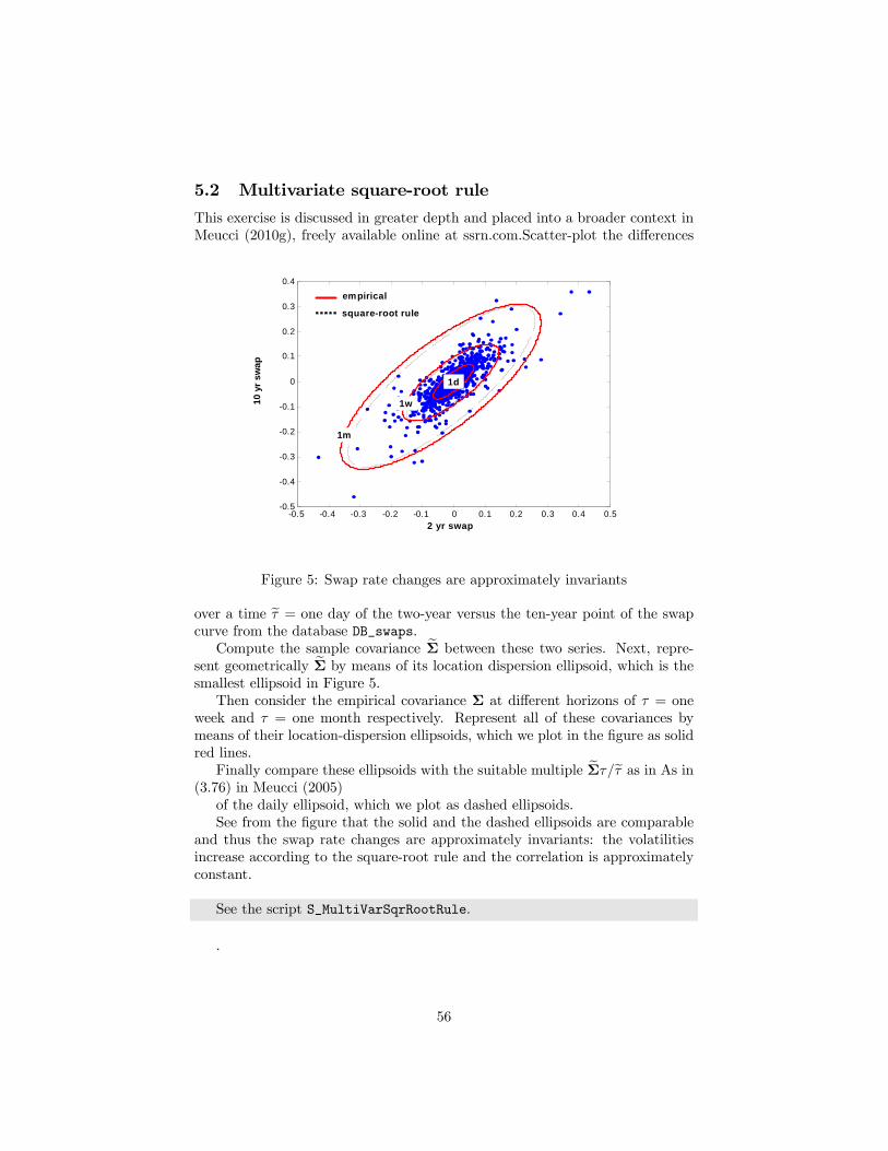
5.2 Multivariate square-root rule
This exercise is discussed in greater depth and placed into a broader context inMeucci (2010g), freely available online at ssrn.com.Scatter-plot the differences
-0.5 -0.4 -0.3 -0.2 -0.1 0 0.1 0.2 0.3 0.4 0.5-0.5
-0.4
-0.3
-0.2
-0.1
0
0.1
0.2
0.3
0.4
2y swap
10y
swap
2 yr swap
10 y
r sw
ap
empirical
square-root rule
1m
1w
1d
Figure 5: Swap rate changes are approximately invariants
over a time eτ = one day of the two-year versus the ten-year point of the swapcurve from the database DB_swaps.Compute the sample covariance eΣ between these two series. Next, repre-
sent geometrically eΣ by means of its location dispersion ellipsoid, which is thesmallest ellipsoid in Figure 5.Then consider the empirical covariance Σ at different horizons of τ = one
week and τ = one month respectively. Represent all of these covariances bymeans of their location-dispersion ellipsoids, which we plot in the figure as solidred lines.Finally compare these ellipsoids with the suitable multiple eΣτ/eτ as in As in
(3.76) in Meucci (2005)of the daily ellipsoid, which we plot as dashed ellipsoids.See from the figure that the solid and the dashed ellipsoids are comparable
and thus the swap rate changes are approximately invariants: the volatilitiesincrease according to the square-root rule and the correlation is approximatelyconstant.
See the script S_MultiVarSqrRootRule.
.
56
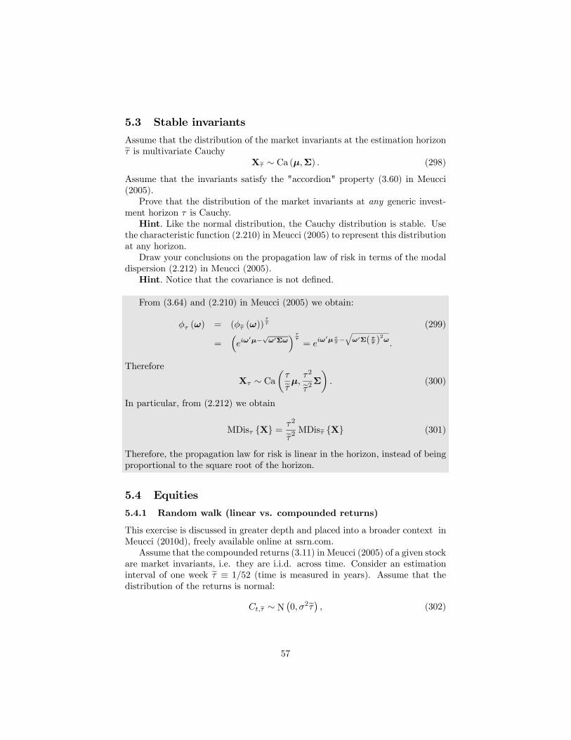
5.3 Stable invariants
Assume that the distribution of the market invariants at the estimation horizoneτ is multivariate CauchyXτ ∼ Ca (µ,Σ) . (298)
Assume that the invariants satisfy the "accordion" property (3.60) in Meucci(2005).Prove that the distribution of the market invariants at any generic invest-
ment horizon τ is Cauchy.Hint. Like the normal distribution, the Cauchy distribution is stable. Use
the characteristic function (2.210) in Meucci (2005) to represent this distributionat any horizon.Draw your conclusions on the propagation law of risk in terms of the modal
dispersion (2.212) in Meucci (2005).Hint. Notice that the covariance is not defined.
From (3.64) and (2.210) in Meucci (2005) we obtain:
φτ (ω) = (φτ (ω))ττ (299)
=³eiω
0µ−√ω0Σω
´ ττ
= eiω0µ τ
τ− ω0Σ( ττ )2ω.
Therefore
Xτ ∼ Caµτeτ µ, τ2eτ2Σ
¶. (300)
In particular, from (2.212) we obtain
MDisτ {X} =τ2eτ2 MDisτ {X} (301)
Therefore, the propagation law for risk is linear in the horizon, instead of beingproportional to the square root of the horizon.
5.4 Equities
5.4.1 Random walk (linear vs. compounded returns)
This exercise is discussed in greater depth and placed into a broader context inMeucci (2010d), freely available online at ssrn.com.Assume that the compounded returns (3.11) in Meucci (2005) of a given stock
are market invariants, i.e. they are i.i.d. across time. Consider an estimationinterval of one week eτ ≡ 1/52 (time is measured in years). Assume that thedistribution of the returns is normal:
Ct,τ ∼ N¡0, σ2eτ¢ , (302)
57
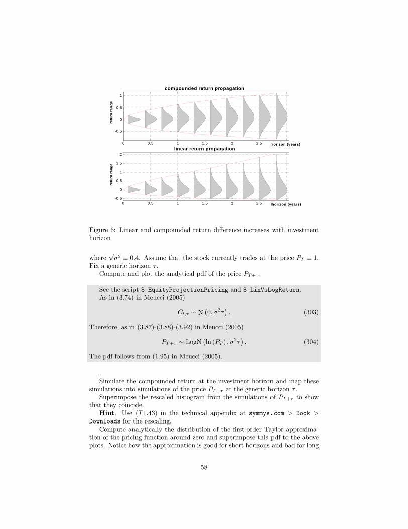
0 0.5 1 1.5 2 2.5 3
-0.5
0
0.5
1
0 0.5 1 1.5 2 2.5 3-0.5
0
0.5
1
1.5
2
compounded return propagation
horizon (years)
horizon (years)
linear return propagation
retu
rn ra
nge
retu
rn ra
nge
Figure 6: Linear and compounded return difference increases with investmenthorizon
where√σ2 ≡ 0.4. Assume that the stock currently trades at the price PT ≡ 1.
Fix a generic horizon τ .Compute and plot the analytical pdf of the price PT+τ .
See the script S_EquityProjectionPricing and S_LinVsLogReturn.As in (3.74) in Meucci (2005)
Ct,τ ∼ N¡0, σ2τ
¢. (303)
Therefore, as in (3.87)-(3.88)-(3.92) in Meucci (2005)
PT+τ ∼ LogN¡ln (PT ) , σ
2τ¢. (304)
The pdf follows from (1.95) in Meucci (2005).
.Simulate the compounded return at the investment horizon and map these
simulations into simulations of the price PT+τ at the generic horizon τ .Superimpose the rescaled histogram from the simulations of PT+τ to show
that they coincide.Hint. Use (T1.43) in the technical appendix at symmys.com > Book >
Downloads for the rescaling.Compute analytically the distribution of the first-order Taylor approxima-
tion of the pricing function around zero and superimpose this pdf to the aboveplots. Notice how the approximation is good for short horizons and bad for long
58
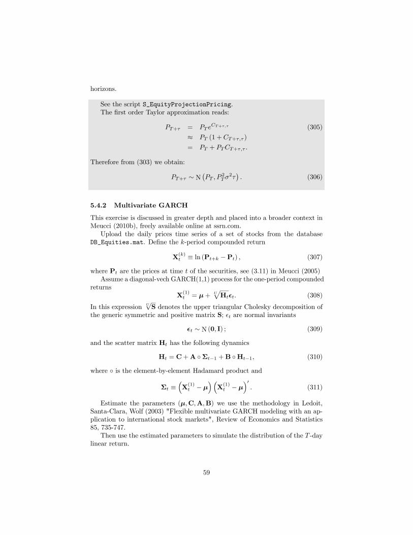
horizons.
See the script S_EquityProjectionPricing.The first order Taylor approximation reads:
PT+τ = PT eCT+τ,τ (305)
≈ PT (1 + CT+τ,τ )
= PT + PTCT+τ,τ .
Therefore from (303) we obtain:
PT+τ ∼ N¡PT , P
2Tσ
2τ¢. (306)
5.4.2 Multivariate GARCH
This exercise is discussed in greater depth and placed into a broader context inMeucci (2010b), freely available online at ssrn.com.Upload the daily prices time series of a set of stocks from the database
DB_Equities.mat. Define the k-period compounded return
X(k)t ≡ ln (Pt+k −Pt) , (307)
where Pt are the prices at time t of the securities, see (3.11) in Meucci (2005)Assume a diagonal-vech GARCH(1,1) process for the one-period compounded
returnsX(1)t = µ+ U
pHt²t. (308)
In this expression U√S denotes the upper triangular Cholesky decomposition of
the generic symmetric and positive matrix S; t are normal invariants
²t ∼ N(0, I) ; (309)
and the scatter matrix Ht has the following dynamics
Ht = C+A ◦Σt−1 +B ◦Ht−1, (310)
where ◦ is the element-by-element Hadamard product and
Σt ≡³X(1)t − µ
´³X(1)t − µ
´0. (311)
Estimate the parameters (µ,C,A,B) we use the methodology in Ledoit,Santa-Clara, Wolf (2003) "Flexible multivariate GARCH modeling with an ap-plication to international stock markets", Review of Economics and Statistics85, 735-747.Then use the estimated parameters to simulate the distribution of the T -day
linear return.
59
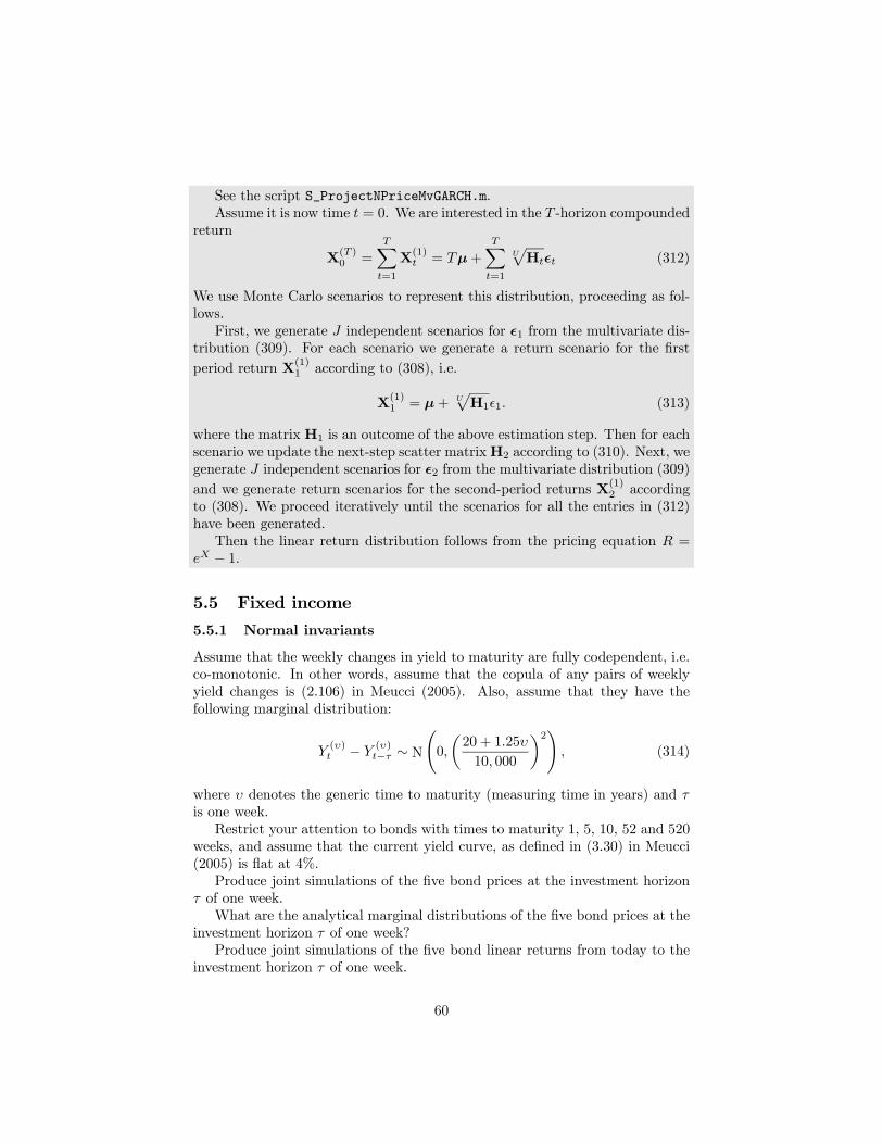
See the script S_ProjectNPriceMvGARCH.m.Assume it is now time t = 0. We are interested in the T -horizon compounded
return
X(T )0 =
TXt=1
X(1)t = Tµ+
TXt=1
UpHt²t (312)
We use Monte Carlo scenarios to represent this distribution, proceeding as fol-lows.First, we generate J independent scenarios for ²1 from the multivariate dis-
tribution (309). For each scenario we generate a return scenario for the firstperiod return X(1)
1 according to (308), i.e.
X(1)1 = µ+ U
pH1 1. (313)
where the matrix H1 is an outcome of the above estimation step. Then for eachscenario we update the next-step scatter matrixH2 according to (310). Next, wegenerate J independent scenarios for ²2 from the multivariate distribution (309)and we generate return scenarios for the second-period returns X(1)
2 accordingto (308). We proceed iteratively until the scenarios for all the entries in (312)have been generated.Then the linear return distribution follows from the pricing equation R =
eX − 1.
5.5 Fixed income
5.5.1 Normal invariants
Assume that the weekly changes in yield to maturity are fully codependent, i.e.co-monotonic. In other words, assume that the copula of any pairs of weeklyyield changes is (2.106) in Meucci (2005). Also, assume that they have thefollowing marginal distribution:
Y(υ)t − Y
(υ)t−τ ∼ N
Ã0,
µ20 + 1.25υ
10, 000
¶2!, (314)
where υ denotes the generic time to maturity (measuring time in years) and τis one week.Restrict your attention to bonds with times to maturity 1, 5, 10, 52 and 520
weeks, and assume that the current yield curve, as defined in (3.30) in Meucci(2005) is flat at 4%.Produce joint simulations of the five bond prices at the investment horizon
τ of one week.What are the analytical marginal distributions of the five bond prices at the
investment horizon τ of one week?Produce joint simulations of the five bond linear returns from today to the
investment horizon τ of one week.
60

What are the analytical marginal distributions of the five bond linear returnsat the investment horizon τ of one week?Comment on why the return on the price of a bond cannot be an invariant.Hints1. Since the market is fully codependent you will only need one uniformly
generated sample2. You will need the quantile function to generate simulations. Compute
the quantile function using interp1, the linear interpolation/extrapolation ofthe cdf.3. For a generic bond with time to maturity υ from the decision date T
the expiry date is E ≡ T + υ. As in (3.81) in Meucci (2005) the price at theinvestment horizon of that bond reads:
Z(T+υ)T+τ = Z
(T+υ−τ)T exp
³− (υ − τ)∆τY
(υ−τ)´. (315)
In other words, the price is determined by the market invariant, a randomvariable, and the known price of a different bond with shorter time to maturity.4. The distribution of the 4-week-to-maturity bond at the 4-week-horizon is
degenerate, i.e. its pdf is the Dirac delta, because the outcome is deterministic.Make sure that your outcome is consistent with this statement.5. See hints for Exercise 5.5.2
See the script S_BondProjectionPricingNormal.From (315) the bond price reads
Z(T+υ)T+τ = eX , (316)
whereX ≡ ln
³Z(T+υ−τ)T
´− (υ − τ)∆τY
(υ−τ). (317)
From (314)∆τY
(υ) ∼ N¡0, σ2υ
¢, (318)
where
σ2υ ≡µ20 + 1.25υ
10, 000
¶2. (319)
ThereforeX ∼ N
³ln³Z(T+υ−τ)T
´, (υ − τ)2 σ2υ−τ
´, (320)
which with (316) implies
Z(T+υ)T+τ ∼ LogN
³ln³Z(T+υ−τ)T
´, (υ − τ)
2σ2υ−τ
´. (321)
From (3.10) in Meucci (2005) the linear return from the current time T tothe investment horizon T + τ of a bond that matures at E ≡ T +υ is defined as
L(T+υ)T+τ,τ ≡
Z(T+υ)T+τ
Z(T+υ)T
− 1. (322)
61
Proceeding as aboveLT+τ,τ = eY − 1, (323)
whereY ≡ ln
³Z(T+υ−τ)T
´− ln
³Z(T+υ)T
´− (υ − τ)∆τY
(υ−τ), (324)
and thus
1 + L(T+υ)T+τ,τ ∼ LogN
³ln³Z(T+υ−τ)T
´− ln
³Z(T+υ)T
´, (υ − τ)
2σ2υ−τ
´, (325)
or L(T+υ)T+τ,τ is a shifted lognormal random variable.Notice that for υ ≡ τ the above distribution is degenerate, i.e. deterministic,
whereas any estimation would have yielded a non-degenerate distribution.
5.5.2 Student t invariants
Consider a fixed-income market, where the changes in yield-to-maturity, or ratechanges, are the market invariants.Assume that the weekly changes in yield for all maturities are fully codepen-
dent, i.e. co-monotonic. In other words, assume that the copula of any pairsof weekly yield changes is (2.106) in Meucci (2005). Assume that the marginaldistributions of the weekly changes in yield for all maturities are:
∆τY(υ) ∼ St
¡ν, µ, σ2υ
¢. (326)
In this expression υ denotes the time to maturity (in years) and
ν ≡ 8, µ ≡ 0,pσ2υ ≡
µ20 +
5
4υ
¶× 10−4. (327)
Consider bonds with current times to maturity 4, 5, 10, 52 and 520 weeks, andassume that the current yield curve, as defined in (3.30) in Meucci (2005) is flatat 4% (measuring time in years).Use the function ProjectionT that takes as inputs the estimation parame-
ters of the t-distributed invariants and the horizon-to-estimation ratio τ/eτ tocompute the cdf of the invariants at the investment horizon τ . You do notneed to know how this function works. Make sure you properly compute thenecessary inputs (see hints below).Use the cdf obtained above to generate a joint simulation of the bond prices
at the investment horizon τ of four weeks.Plot the histogram of the linear returns LT+τ,τ of each bond over the in-
vestment horizon, where the linear return is defined consistently with (3.10) inMeucci (2005) as follows:
Lt,τ ≡Z(E)t
Z(E)t−τ− 1. (328)
Notice that the long-maturity (long duration) bonds are much more volatilethan the short maturity (short duration) bonds.
62
HintsSuppose today is Nov.1 2006 and we hold a zero-coupon bond that matures
in 10 weeks, i.e., it matures on Jan.15. 2007.We are interested in the value of the bond after 4 weeks, i.e., Dec.1 2006.Recall from (3.30) in Meucci (2005) that the value of a zero-coupon bond is
fully determined by its yield to maturity.At the 4-week investment horizon (Dec.1 2006) our originally 10-week bond
will be a 6-week bond. Therefore its price will be fully determined by the valueof the 6-week yield to maturity on Dec.1 2006. For instance, if the 6-weekyield to maturity on Dec.1 2006 is 4.1%, then in (3.30) we have υ ≡ 6/52 andY(6/52)12/1/2006 ≡ 0.041. Therefore the bond price on Dec.1 2006 will be:
Z1/15/200712/1/2006 = exp
µ− 652
Y(6/52)12/1/2006
¶(329)
= e−652×0.041 ≈ 0.99528.
To summarize, in order to price the 10-week bond at the 4-week investmenthorizon we need the distribution of the 6-week yield to maturity on Dec.1 2006.In order to proceed, we recall that in the zero-coupon bond world, the in-
variants are the non-overlapping changes in yield to maturity, for any yield tomaturity, see the textbook from pp.109 to pp.113. In particular, from (3.31) inMeucci (2005), the following four random variables are i.i.d.:
X1 ≡ Y(6/52)11/08/2006 − Y
(6/52)11/1/2006 (330)
X2 ≡ Y(6/52)11/15/2006 − Y
(6/52)11/08/2006 (331)
X3 ≡ Y(6/52)11/22/2006 − Y
(6/52)11/15/2006 (332)
X4 ≡ Y(6/52)12/1/2006 − Y
(6/52)11/22/2006 (333)
Notice that we can express the random variable Y (6/52)12/1/2006 in (329) as follows:
Y(6/52)12/1/2006 = Y
(6/52)11/1/2006 +X1 +X2 +X3 +X4. (334)
Substituting this in (329) we obtain
Z1/15/200712/1/2006 = e
− 652 Y
(6/52)11/1/2006
+X1+X2+X3+X4 (335)
= Z12/15/200611/1/2006 e−6/52(X1+X2+X3+X4),
where in the last row we used (3.30) in Meucci (2005) again. This expression is(315).The term Z
12/15/200611/1/2006 is the current value of a 6-week zero-coupon bond,
which is known. Indeed, using the information that the curve is currently flatat 4% we obtain:
Z12/15/200611/1/2006 = e
− 652Y
(6/52)11/1/2006 = e−
652×0.04 ≈ 0.99540. (336)
63
We are left with the problem of projecting the invariant, i.e. computing thedistribution of X1+X2+X3+X4, and pricing it, i.e. computing the distributionof e−6/52(X1+X2+X3+X4) in (335).To project the invariant we need to compute the distribution of the sum four
independent t variables
X1d= X2
d= X3
d= X4 ∼ St
³ν, µ, σ26/52
´, (337)
where the parameters follow from (326). This is the FFT algorithm provided inProjectionT. The pricing is then performed by Monte Carlo simulations.As for the linear returns, these are the return on our bond over the invest-
ment horizon. Therefore (328) reads:
L12/1/2006, 452 ≡Z(1/15/2007)12/1/2006
Z(1/15/2007)11/1/2006
− 1. (338)
See the script S_BondProjectionPricingT.
5.6 Derivatives
Consider a market of call options on the S&P 500, with current time to maturityof 100, 150, 200, 250, and 300 days and strikes equal 850, 880, 910, 940, and970 respectively. Assume that the investment horizon is 8 weeks.Consider the time series of the underlying and the implied volatility surface
provided in DB_ImplVol. Fit a joint normal distribution to the weekly invari-ants, namely the log-changes in the underlying and the residuals from a vectorautoregression of order one in the log-changes in the implied volatilities surfaceσt. µ
lnSt+τ − lnStlnσt+τ − lnσt
¶∼ N(τµ, τΣ) (339)
Hint. See Exercise 3.2.3: here we are assuming for simplicity that the invariantsare the log-changes in the implied volatility surface instead of the the residu-als from a vector autoregression of order one on the same variables. Noticehow (339) represents a special case of Exercise 3.2.3, which we assume here forsimplicity.Generate simulations for the invariants and jointly project underlying and
implied volatility surface to the investment horizon.Price the above simulations through the full Black-Scholes formula at the
investment horizon, assuming a constant risk-free rate at 4%.Hint. You need to interpolate the surface at the proper strike and time tomaturity, which at the horizon has shortened.Compute the joint distribution of the linear returns of the call options, as
represented by the simulations: the current prices of the options can be obtainedsimilarly to the prices at the horizon by assuming that the current values ofunderlying and implied volatilities are the last observations in the database.
64
For each call option, plot the histogram of its distribution at the horizonand the scatter-plot of its distribution against the underlying.Verify what happens as the investment horizon shifts further in the future.
See the script S_CallsProjectionPricing.
6 Dimension reduction
6.1 "Pure residual" models: duration/curve attribution
This exercise is discussed in greater depth and placed into a broader context inMeucci (2010f), freely available online at ssrn.com.Consider as market Xt the weekly linear returns of N ≡ 3 bonds, net of
the "carry", or "roll-down", i.e. the deterministic component as in (3.108) andcomments thereafter in Meucci (2005). Consider as exogenous factors Ft theweekly changes in K ≡ 9 key rates of the government curve: 6 months, one year,2, 3, 5, 7 10, 20 and 30 years. Consider as exogenous loadings Bt the key ratedurations of these bonds, where Bt is a N ×K = 3× 9 matrix.Consider the pure residual factor model
Xt ≡ BtFt +Ut. (340)
Find in the database db_BondAttribution the time series over the year 2009of the above variables. Model the joint distribution of the yet-to-be realizedfactors and residuals by means of the empirical distribution
fFT+!,UT+!≡ 1
T
TXt=1
δ(ft,ut), (341)
see (4.35) in Meucci (2005).Compute the correlation among residuals and between factors and residuals
according to the empirical distribution (341) and verify that (340) is not asystematic-plus-idiosyncratic model, see Figure 7.
See script S_PureResidualBonds
6.2 "Time series" or "macroeconomic" factor models
6.2.1 Unconstrained time series correlations and r-square
This exercise is discussed in greater depth and placed into a broader context inMeucci (2010f), freely available online at ssrn.com.Consider the approximation Y provided to the market X by a given model
X ≡ Y +U, (342)
65
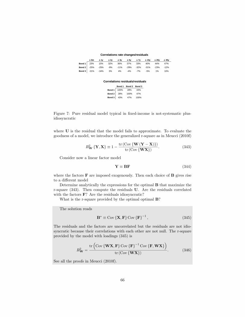
10%1%-5%-7%-4%4%3%-34%-31%Bond 3
-12%-23%-31%-32%-29%-11%-9%-25%-25%Bond 2
47%44%40%33%37%36%32%15%23%Bond 1
∆ 30y∆ 20y∆ 10y∆ 7y∆ 5y∆ 3y∆ 2y∆ 1y∆ 6m
100%47%43%Bond 3
47%100%28%Bond 2
43%28%100%Bond 1
Bond 3Bond 2Bond 1
Correlations rate changes/residuals
Correlations residuals/residuals
Figure 7: Pure residual model typical in fixed-income is not-systematic plus-idiosyncratic
where U is the residual that the model fails to approximate. To evaluate thegoodness of a model, we introduce the generalized r-square as in Meucci (2010f)
R2W {Y,X} ≡ 1− tr (Cov {W (Y −X)})tr (Cov {WX}) . (343)
Consider now a linear factor model
Y ≡ BF (344)
where the factors F are imposed exogenously. Then each choice of B gives riseto a different modelDetermine analytically the expressions for the optimal B that maximize the
r-square (343). Then compute the residuals U. Are the residuals correlatedwith the factors F? Are the residuals idiosyncratic?What is the r-square provided by the optimal optimal B?
The solution reads
B∗ ≡ Cov {X,F}Cov {F}−1 , (345)
The residuals and the factors are uncorrelated but the residuals are not idio-syncratic because their correlations with each other are not null. The r-squareprovided by the model with loadings (345) is
R2W =tr³Cov {WX,F}Cov {F}−1Cov {F,WX}
´tr (Cov {WX}) . (346)
See all the proofs in Meucci (2010f).
66
6.2.2 Unconstrained time series industry factors
This exercise is discussed in greater depth and placed into a broader context inMeucci (2010f), freely available online at ssrn.com. Also, compare with Exercise6.2.1 and Exercise 6.2.3.Consider the n = 1, . . . , N ≈ 500 stocks in the S&P 500 and the k =
1, . . . ,K ≡ 10 industry indices. We intend to build a factor model
X = a+BF+U, (347)
where X ≡ (X1, . . . ,XN )0 are the yet to be realized returns of the stocks over
next week; a ≡ (a1, . . . , aN )0 are N constants; F ≡ (F1, . . . , FK)0 are the factors,i.e. the yet to be realized returns of the industry indices over next week; B is aN ×K matrix of coefficients that transfers the randomness of the factors intothe randomness of the risk drivers; and U ≡ (U1, . . . , UN )0 are defined as the Nresiduals that make (347) an identity.Upload the database of the weekly stock returns {xt}t=1,...,T , and the data-
base of the simultaneous weekly indices returns {ft}t=1,...,T . Model the jointdistribution of X and F by means of the empirical distribution
fX,F ≡1
T
TXt=1
δ(xt,ft), (348)
where δ(y) denotes the Dirac-delta, which concentrates a unit probability masson the generic point y.Compute the optimal loadings B∗ in (347) that give the factor model the
highest generalized multivariate distributional r-square as in Meucci (2010f)(you will notice that the weights are arbitrary)
B∗ ≡ argmaxB
R2W {BF,X} . (349)
Compute the correlations of the residuals with the factors and verify that it isnull. Then compute the correlations of the residuals with each other and verifythat it is not null, i.e. the residuals are not idiosyncratic.Hint: the optimal loadings turn out to be the standard multivariate OLS,
see the proof in Meucci (2010f).
See script S_TimeSeriesIndustries
6.2.3 Generalized time-series industry factors
This exercise is discussed in greater depth and placed into a broader context inMeucci (2010f), freely available online at ssrn.com. Consider the same frame-work as in Exercise 6.2.2. Compute as in that exercise the optimal loadings B∗
in (347) that give the factor model the highest constrained generalized multi-variate distributional r-square defined in Meucci (2010f)
B∗ ≡ argmaxB∈C
R2W {BF,X} . (350)
67
In this expression, assume that the constraints C are the following: all the load-ings are bound from below by B ≡ 0.8 and from above by B ≡ 1.2 and themarket-capitalization weighted sum of the loadings be one
0.8 ≤ Bn,k ≤ B, n = 1, . . . ,N, k = 1, . . . ,K (351)NXn=1
MnBn,k ≡ 1. (352)
Proxy the market capitalization as equal weights for this exercise.Then compute the correlations of the residuals among each other and with
the factors and verify that neither is null. In other words, the model is not ofsystematic-plus-idiosyncratic type.
See script S_TimeSeriesConstrainedIndustries
6.2.4 Analysis of residual
Consider a market of N stocks, where each stock n = 1, . . . , N trades at time tat the price Pt,n. Consider as interpretation factors the linear returns on a setof K indices, such as GICS sectors, where each index k = 1, . . . ,K quotes attime t at the price St,k.As in Black-Scholes, assume that stocks and indices follow a geometric
Brownian motion, i.e.µXF
¶∼ N
µτ
µµXµF
¶, τ
µΣX ΣXF
Σ0XF ΣF
¶¶, (353)
where
Xn ≡ ln
µPT+τ,nPT,n
¶(354)
Fk ≡ ln
µST+τ,kST,k
¶. (355)
We want to represent the linear returns on the securities
R = eX − 1 (356)
in terms of the explanatory factors
Z = eF − 1 (357)
by means of a linear modelR ≡ BZ+U. (358)
Compute the expression of B that minimizes the generalized r-square, theexpression of the covariance ΣZ of the explanatory factors and the expressionof the covariance ΣU of the residuals.
68
From (3.121) the optimal loadings read:
B ≡ E©RZ0
ª ¡E©ZZ0
ª¢−1. (359)
Also from (2.219)-(2.220) in general for a log-normal variable
Y ∼ LogN (µ,Σ) . (360)
then
E {Y} = eµ+12 diag(Σ). (361)
E©YY0ª =
³e(µ+
12 diag(Σ))e(µ+
12 diag(Σ))0
´◦ eΣ, (362)
where ◦ denotes the term-by-term Hadamard product.Since
1 +
µRZ
¶∼ LogN
µτ
µµXµF
¶, τ
µΣX ΣXF
Σ0XF ΣF
¶¶, (363)
using (361), (362) and the property
E {(Y − 1)} = E {Y}− 1 (364)
E©(Y − 1) (Y − 1)0
ª= E
©YY0ª+ 110 − E©Y10ª− E©1Y0ª . (365)
we can easily compute all the terms E {R}, E©RR0ª, E {Z}, E©ZZ0ª and
E©RZ0
ª.
Therefore we obtain the loadings (359). The covariance of the explanatoryfactors then follows from
ΣZ = E©ZZ0
ª− E {Z}E {Z0} (366)
and similarly the covariance of the returns follows from
ΣR = E©RR0ª− E {R}E {R0} (367)
Generate randomly the parameters of the distribution (353). Then generatea large number of Monte Carlo scenarios from (353) and verify that the samplecovariances of explanatory factors and linear returns match with (366) and (367).Estimate the loadings by OLS of the Monte Carlo simulations i.e. the sample
counterpart of (359). Compute the residuals, and their sample covariance bΣR
and verify that bΣR is not diagonal and thatbΣR 6= bBbΣZbB0 + bΣU . (368)
Now repeat the experiment assuming that one of the factor is non-random,
69
by setting the respective volatility to zero in (353) and verify that
bΣR ≡ bBbΣZbB0 + bΣU . (369)
In this case the most explanatory interpretation reads
R ≡ a+BZ+U, (370)
where the OLS loadings are
B ≡ ΣRZΣ−1ZZ (371)
anda ≡ E {R}−BE {Z} (372)
See script S_ResidualAnalysisTheory
Now repeat the experiment assuming that all the factors are random, butenforcing E {Z} ≡ 0 by suitably setting the drift µF in (353) as a function ofthe diagonal of ΣF and verify again thatbΣR ≡ bBbΣZ
bB0 + bΣU . (373)
See script S_ResidualAnalysisTheory
Important: notice that under no circumstance is the residual covariancematrix bΣU diagonal. This issue is discussed in greater depth and placed into abroader context in Meucci (2010f), freely available online at ssrn.com.
6.3 "Cross-section" or "fundamental" factor models
6.3.1 Unconstrained cross-section correlations and r-square
This exercise is discussed in greater depth and placed into a broader context inMeucci (2010f), freely available online at ssrn.com.Consider the approximation Y provided to the market X by a given model
X ≡ Y +U, (374)
where U is the residual that the model fails to approximate. To evaluate thegoodness of a model, we introduce the generalized r-square as in Meucci (2010f)
R2W {Y,X} ≡ 1− tr (Cov {W (Y −X)})tr (Cov {WX}) . (375)
Consider now a linear factor model
Y ≡ BF (376)
70
where the loadings B are exogenously chosen, but the factors F are left unspec-ified. Then each choice of F gives rise to a different model. Assume that thefactors are a linear function of the market
F ≡GX. (377)
Determine analytically the expressions for the optimal G that maximize ther-square (375). Then compute the factors F, the explained market Y and theresidual U. Is the market Y explained by the factors orthogonal to the residualU? Is the explained market Y correlated with the residual U? Are the residualidiosyncratic?
The solution readsG∗ = (B0ΦB)
−1B0Φ, (378)
where Φ ≡W0W. Then r-square provided by this solution reads
R2W =tr (Cov {WBF})tr (Cov {WX}) , (379)
see the proof in Meucci (2010f).With (378) the factors (377) read
F ≡ (B0ΦB)−1B0ΦX (380)
and the model-recovered market is
Y ≡ PX, (381)
whereP ≡ B (B0ΦB)−1B0Φ (382)
is a projection operator. Indeed, it is easy to check that P2 = P. The linearassumption (377) gives rise to the residuals
U ≡ P⊥X, (383)
whereP⊥ ≡ I−B (B0ΦB)−1B0Φ (384)
is the projection in the space orthogonal to the span of the model-recoveredmarket. Therefore, the recovered market and the residuals live in orthogonalspaces. However, the residuals and the factors are not uncorrelated and theresiduals are not idiosyncratic, see also the discussion in Meucci (2010f).
6.3.2 Unconstrained cross-section industry factors
This exercise is discussed in greater depth and placed into a broader context inMeucci (2010f), freely available online at ssrn.com. Also, compare with Exercise6.3.1 and Exercise 6.3.3.
71
Consider the n = 1, . . . , N ≈ 500 stocks in the S&P 500 and the k =1, . . . ,K ≡ 10 industry indices. We intend to build a factor model
X = a+BF+U, (385)
where X ≡ (X1, . . . ,XN )0 are the yet to be realized returns of the stocks over
next week; a ≡ (a1, . . . , aN )0 are N constants; F ≡ (F1, . . . , FK)0 are the factors,i.e. the yet to be realized random variables; B is a N ×K matrix of coefficientsthat transfers the randomness of the factors into the randomness of the riskdrivers and that is imposed exogenously; and U ≡ (U1, . . . , UN )0 are defined asthe N residuals that make (347) an identity.Upload the database of the matrixB of dummy exposures of each stock to its
industry. Upload the weekly stock returns {xt}t=1,...,T . Model the distributionof X by means of the empirical distribution
fX ≡1
T
TXt=1
δ(xt), (386)
where δ(y) denotes the Dirac-delta, which concentrates a unit probability masson the generic point y.Define the cross-sectional factors as linear transformation of the market F ≡
GX. Compute the optimal coefficientsG∗ that give the factor model the highestgeneralized multivariate distributional r-square defined in Meucci (2010f)
G∗ ≡ argmaxG
R2W {BGX,X} , (387)
In this expression assume that the r-square weights matrix W to be diagonaland equal to the inverse of the standard deviation of each stock return.Then compute the correlations of the residuals among each other and with
the factors and verify that neither is null. In other words, the model is not ofsystematic-plus-idiosyncratic type.Hint: the optimal loadings turn out to be the standard multivariate weighted-
OLS, see the proof in Meucci (2010f).
See script S_CrossSectionIndustries
6.3.3 Generalized cross-section industry factors
This exercise is discussed in greater depth and placed into a broader context inMeucci (2010f), freely available online at ssrn.com. Consider the same frame-work as in Exercise 6.3.2.Compute similarly to (387) the optimal coefficients G∗ that give the cross-
sectional industry factors the highest generalized multivariate distributional r-square defined in Meucci (2010f), but, unlike in Exercise 6.3.2, add a set ofconstraints C
G∗ ≡ argmaxB∈C
R2W {BGX,X} . (388)
72
In this expression, assume that the constraints C are that the factors F ≡ GXbe uncorrelated with the overall market
C : GCov {X}m ≡ 0, (389)
where you can assume the market weightsm to be equal weights for this exercise.Then compute the correlations of the residuals among each other and with
the factors and verify that neither is null. In other words, the model is not ofsystematic-plus-idiosyncratic type.
See script S_CrossSectionConstrainedIndustries
6.3.4 Comparison cross-section with time-series industry factors
This exercise is discussed in greater depth and placed into a broader contextin Meucci (2010f), freely available online at ssrn.com. Consider the time-seriesindustry factors constructed in Exercise 6.2.2 and the cross-section industryfactors constructed in Exercise 6.3.2. Verify that the time series factors arehighly correlated with their cross-sectional counterparts.
See script S_TimeSeriesVsCrossSectionIndustries in the "cross-section"folder.
6.3.5 Correlation factors-residual: normal example
This exercise is discussed in greater depth and placed into a broader context inMeucci (2010f), freely available online at ssrn.com.Consider an N -dimensional normal market
X ∼ N(µ,Σ) , (390)
and assume that we want to explain it through a linear model
X ≡ bF +U, (391)
where b is a given vector of loadings, F is a yet-to-be defined explanatory factor,and U are residuals that make (391) hold.Choose N and generate arbitrarily the parameters in (390) and the vector
of loadings in (391). Then generate a large number of simulations from (390).Define the factor F through cross-sectional regression and compute the residualsU. Then show that factor and residual are correlated:
Cor {F,U} 6= 0. (392)
See script S_FactorResidualCorrelation
73

6.4 "Statistical" approach: principal component analysis
6.4.1 Matrix algebra
Consider a N ×N matrix of the form
Σ ≡ EΛE0, (393)
where Λ is diagonal and E is invertible.Prove that Σ is symmetric, see definition (A.51) in Meucci (2005).
Σ0 ≡¡EΛE0
¢0= EΛ0E0 = EΛE0 = Σ (394)
Prove that Σ is positive if and only if all the diagonal elements of Λ arepositive, see definition (A.52) in Meucci (2005).
For any v there exists one and only one w ≡ E0v and w ≡ 0 ⇐⇒ v ≡ 0.Assume that all the diagonal elements of Λ are positive and v 6= 0. Then:
v0Σv ≡ v0EΛE0v = w0Λw (395)
=NXn=1
w2nλn > 0.
Similarly, from the above identities, if 0 < v0Σv for any v 6= 0, then each λnhas to be positive.
6.4.2 Location-dispersion ellipsoid and geometry
Consider the ellipsoid
Em,S ≡©x ∈ RN such that (x−m)0 S−1 (x−m) ≤ 1
ª. (396)
What is the geometrical interpretation of m?What is the geometrical interpretation of the eigenvectors of S?What is the geometrical interpretation of the eigenvalues of S?What is the statistical interpretation of (396)?Hint. This is a trick question.
The vector m represents the center of ellipsoid.The eigenvectors are the directions of the principal axes of the ellipsoid.The square root of the eigenvalues are the length of the principal axes of the
ellipsoid.There is no statistical interpretation, as long asm and S are not the expected
value and the covariance matrix respectively of a multivariate distribution.
74

6.4.3 Location-dispersion ellipsoid and statistics
Generate J ≡ 10, 000 simulations from a bi-variate log-t variable:
ln (X) ∼ St (ν,µ,Σ) . (397)
where ν ≡ 40, µ ≈ 0.5 and diag (Σ) ≈ 0.01 (you can choose the off-diagonalelement).Hint. You will have to shift and rescale the output of mvtrnd.Consider the generic versor in the plane:
eθ ≡µcos θsin θ
¶. (398)
Consider the random variable Zθ ≡ e0θX, namely the projection of X on thedirection eθ. Compute and plot the sample standard deviation σθ of Zθ as afunction of θ ∈ [0, π] (select a grid of 100 points).Show in a figure that the minimum and the maximum of σθ are provided by
versors parallel to the principal axes of the ellipsoid defined by the sample meanm and the sample covariance S as plotted by the function TwoDimEllipsoid.Compute the radius rθ, i.e. the distance between the surface of the ellipsoid
and the center of the ellipsoid along the direction of the versor as a function ofθ ∈ [0, π] (select a grid of 100 points).Hint. To compute rθ notice that it satisfies:
(rθeθ)0 S−1 (rθeθ) = 1. (399)
In a separate figure superimpose the plot of σθ and the plot of rθ, showingthat the minimum and the maximum of σθ (i.e. the minimum and the maximumvolatility), correspond to the the minimum and the maximum of rθ respectively(i.e. the length of the smallest and largest principal axis). Notice that the radiusequals the standard deviation only on the principal axes.
See the script S_MaxMinVariance.
6.4.4 PCA derivation, correlations and r-square
This exercise is discussed in greater depth and placed into a broader context inMeucci (2010f), freely available online at ssrn.com.Consider the approximation Y provided to the market X by a given model
X ≡ Y +U, (400)
where U is the residual that the model fails to approximate. To evaluate thegoodness of a model, we introduce the generalized r-square as in Meucci (2010f)
R2W {Y,X} ≡ 1− tr (Cov {W (Y −X)})tr (Cov {WX}) . (401)
75
Consider now a linear factor model
Y ≡ BF (402)
where the factors are extracted by linear combinations from the market
F ≡GX (403)
Then each choice of B and G gives rise to a different model Y. Determineanalytically the expressions for the optimal B and G that maximize the r-square (401) and verify that they are the principal components of the matrixCov {WX}. What is the r-square provided by the optimal optimal B and G?Then compute the residuals U. Are the residuals correlated with the factors F?Are the residuals idiosyncratic?
First, we perform the spectral decomposition of the covariance matrix
Cov {WX} ≡ EΛE0. (404)
In this expressionΛ is the diagonal matrix of the decreasing, positive eigenvaluesof the covariance:
Λ ≡ diag¡λ21, . . . , λ
2N
¢; (405)
and E is the juxtaposition of the respective eigenvectors, which are orthogonaland of length 1 and thus EE0 = IN :
E ≡³e(1), . . . , e(N)
´, (406)
Next, we define a N ×K matrix as the juxtaposition of the first K eigenvectors
EK ≡³e(1), . . . , e(K)
´. (407)
Then optimal B and G read
B∗ =W−1EK , G∗ ≡ E0KW. (408)
The r-square (387) provided by the principal component solution (408) reads
R2W =
PKk=1 λ
2kPN
n=1 λ2n
. (409)
The residuals are not correlated with the factors F but they are correlated with
each other and therefore they are not idiosyncratic. See all the proofs in Meucci(2010f).
76
6.4.5 PCA and projection
Prove that the PCA-recovered market (3.160) in Meucci (2005) represents theorthogonal projection of the original market onto the hyperplane generated bythe first K eigenvectors stemming from the expectation of the original market.
See the Technical Appendix www.3.5.
6.4.6 PCA of two-point swap curve
Upload the database DB_Swap2y4y of the 2yr and 4yr daily par swap rates.Plot the "current curve" i.e. the rates at the last observation date as func-
tions of the respective maturities ("points on the curve").Find the two invariants for the two rate series for a weekly estimation horizon
(one week = five days). Use the RunAnalysis test.Scatter plot the time series of one invariant against the time series of the
other invariant.Superimpose the two-dimensional location-dispersion ellipsoid determined
by sample mean and sample covariance of the invariants (set the scale factorequal to 2): you should see a highly elongated ellipsoid.Perform the spectral decomposition of the sample covariance of the invari-
ants.Plot the two entries of the first eigenvector (first factor loadings) as a function
of the respective points on the curve.Superimpose the plot of the two entries of the second eigenvector (second
factor loadings) as a function of the respective points on the curve.Compute and plot a one-standard-deviation effect and a minus-one-standard-
deviation effect of the first factor on the current curve as in the case study inthe textbook.Compute and plot a one-standard-deviation effect and a minus-one-standard-
deviation effect of the second factor on the current curve, as in the case studyin the textbook.Compute the generalized R2 provided by the first factor.Compute the generalized R2 provided by both factors.
See the script S_SwapPCA2Dim.
6.4.7 Eigenvectors for Toeplitz structure
Write a script that generates a N × N Toeplitz matrix with structure as in(3.209)-(3.214)-(3.222) in Meucci (2005), i.e.
Sj,j+k ≡ r|k|, (410)
where 0 < r < 1.Hint. Use the command diag.
77
Show in a figure that the eigenvectors have a Fourier basis structure as in(3.217) in Meucci (2005).
See the script S_Toepliz.
6.4.8 Generalized principal component analysis
This exercise is discussed in greater depth and placed into a broader context inMeucci (2010f), freely available online at ssrn.com. Also, compare with Exericse6.2.4. ???
6.5 "Statistical" approach: factor analysis puzzle
This exercise is discussed in greater depth and placed into a broader contextin Meucci (2010f), freely available online at ssrn.com, to which we refer for theexplanation of the puzzle below.Consider a N -dimensional market that is normally distributed
X ∼ N(µ,Σ) , (411)
Choose an arbitrary dimension N and generate µ arbitrarily. Then generate Σas follows
Σ ≡ BB0 +∆2 (412)
where B is an arbitrary matrix N × K, with K < N and ∆2 is an arbitrarydiagonal matrix.Generate a large number of scenarios {xj}j=1,...,J from the distribution (411)
with matching sample first and second moment bµ and bΣ, as in Exercise 1.2.3.Run the built-in MATLAB function factoran, which outputs the estimated
values of bB and b∆ as well as the hidden factors {fj}j=1,...,J .Verify that the factor analysis routine works well, i.e.
bΣ ≡ bBbB0 + b∆2. (413)
Compute the residuals uj ≡ xj −Bf j and their sample covariance.Verify that the residuals are not idiosyncratic, in contradiction with the very
principles of factor analysis.
See the script S_FactorAnalysisNotOK.
6.6 "Factors on Demand"
6.6.1 Horizon effect
This exercise is discussed in greater depth and placed into a broader context inMeucci (2010c) and Meucci (2010b), both freely available online at ssrn.com.
78
Consider as in Exercise 6.2.4 a market of N stocks, where each stock n =1, . . . ,N trades at time t at the price Pt,n. Consider as interpretation factorsthe linear returns on a set of K indices, such as GICS sectors, where each indexk = 1, . . . ,K quotes at time t at the price St,k.As in Black-Scholes, assume that stocks and indices follow a geometric
Brownian motion, i.e.µXF
¶∼ N
µτ
µµXµF
¶, τ
µΣX ΣXF
Σ0XF ΣF
¶¶, (414)
where
Xn ≡ ln
µPT+τ,nPT,n
¶(415)
Fk ≡ ln
µST+τ,kST,k
¶. (416)
In particular, assume that the compounded returns are generated by the linearmodel
X ≡ τµX +DF+ ², (417)
where D is a constant matrix of loadings,µF²
¶∼ N
µµ00
¶,
µτΣF 00 τΣ
¶¶, (418)
and Σ is diagonal. Notice that (417)-(418) is a specific case of, and fullyconsistent with, the more general formulation (414). The specification (417) isthe "estimation" side of the model, i.e. the model that would be fitted to theempirical observations.We want to represent the linear returns on the securities
R = eX − 1 (419)
in terms of the explanatory factors
Z = eF − 1 (420)
by means of a linear model
R ≡ a+BZ+U. (421)
The specification (421) is the interpretation side of the model, i.e. the modelthat would be used for portfolio management applications, such as hedging orstyle analysis.Upload µX, D, ΣF and Σ from db_LinearModel and study the relation-
ship between the constant τµX in (417) and the intercept a in (421) and therelationship between the loadings D in (417) and the loadings B in (421).
79
See script S_HorizonEffectIn particular, in the simple bi-variate case and rescaling for simplicity such
that Pt = St = 1 the returns are shifted multivariate lognormalÃR(t)P
R(t)S
!∼ LogN
µt
∙µXµF
¸, t
∙σ2X ρX,FσXσF
ρX,FσXσF σ2F
¸¶− 1, (422)
We recall from (2.219)-(2.220) in Meucci (2005) that in general if
Y ∼ LogN (µ,Σ) . (423)
then
E {Y} = eµ+12 diag(Σ). (424)
E©YY0ª =
³e(µ+
12 diag(Σ))e(µ+
12 diag(Σ))0
´◦ eΣ (425)
AlsoCov {Y} = E
©YY0ª− E {Y}E {Y0} . (426)
From (3.127) in Meucci (2005) the beta in (421) simplifies as
β ≡Cov
nR(t)P , R
(t)S
oVar
nR(t)S
o . (427)
Therefore
β =
³eµXt+σ
2Xt/2+µF t+σ
2F t/2
´ ¡eρX,FσXσF t − 1
¢e2µF t+σ
2F t¡eσ
2F t − 1
¢ . (428)
Is U idiosyncratic?
It is not, and the longer the horizon, the more pronounced this effect, seescript S_HorizonEffect.
6.6.2 No-Greek hedging
This exercise is discussed in greater depth and placed into a broader context inMeucci (2010c), see also Meucci (2010b), both freely available online at ssrn.com.Consider the market of call options on the S&P 500 described in Exercise
5.6, namely call options on the S&P 500, with current time to maturity of100, 150, 200, 250, and 300 days and strikes equal 850, 880, 910, 940, and 970respectively.Consider the time series of the underlying and the implied volatility surface
provided in DB_ImplVol. Fit a joint normal distribution to the weekly invari-ants, namely the log-changes in the underlying and the residuals from a vector
80
autoregression of order one in the log-changes in the implied volatilities surfaceσt. µ
lnSt+τ − lnStlnσt+τ − lnσt
¶∼ N(τµ, τΣ) (429)
Assume that the investment horizon is 8 weeks. We want to represent the linearreturns on the options RC in terms of the linear returns R of the underlyingS&P 500 by means of a linear model
RC ≡ a+ bR+U. (430)
Notice that the specification (430) is the interpretation side of a "factors ondemand" model.Generate joint simulations for RC and R as in Exercise 5.6 and scatter-plot
the results. Then compute a and b by OLS.Compute the cash and underlying amounts necessary to hedge RC based on
the delta of the Black-Scholes formula and compare with a and b.Repeat the above exercise when the investment horizon shifts further or
closer in the future.
See script S_FODHedgeOptions.To compute the hedge, consider the risk-neutral pricing equation for a generic
option (not necessarily a call option)
∆O − δ∆S ≈ Cr∆t, (431)
where O is the option price; S is the underlying value; r is the risk-free rate; δis the "delta"
δ ≡ ∂O
∂S; (432)
and C is the cash amount:C ≡ O − δS. (433)
Then∆O
O≈ C
Or∆t+
δ
OS∆S
S(434)
orRO ≈ a+ bR, (435)
where
a ≡ C
Or∆t, b ≡ δ
OS. (436)
6.6.3 Selection heuristics
This exercise is discussed in greater depth in the context of Factors on Demandin Meucci (2010c), freely available online at ssrn.com.
81
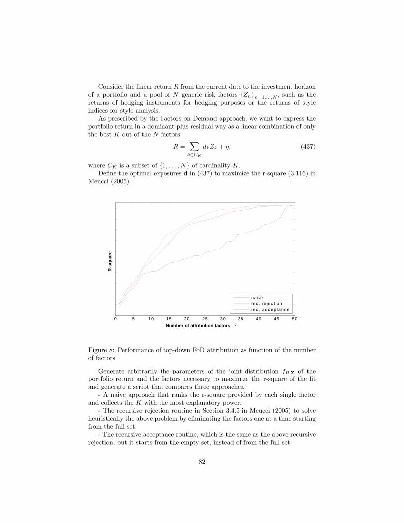
Consider the linear return R from the current date to the investment horizonof a portfolio and a pool of N generic risk factors {Zn}n=1,...,N , such as thereturns of hedging instruments for hedging purposes or the returns of styleindices for style analysis.As prescribed by the Factors on Demand approach, we want to express the
portfolio return in a dominant-plus-residual way as a linear combination of onlythe best K out of the N factors
R =Xk∈CK
dkZk + η, (437)
where CK is a subset of {1, . . . , N} of cardinality K.Define the optimal exposures d in (437) to maximize the r-square (3.116) in
Meucci (2005).
0 5 10 15 20 25 30 35 40 45 500
5
10
15
20
25
30
35
40
45
50
num p lay ers out o f to ta l 50
na iverec . re jec t ionrec . ac c eptanc e
Number of attribution factors
R-s
quar
e
Figure 8: Performance of top-down FoD attribution as function of the numberof factors
Generate arbitrarily the parameters of the joint distribution fR,Z of theportfolio return and the factors necessary to maximize the r-square of the fitand generate a script that compares three approaches.- A naive approach that ranks the r-square provided by each single factor
and collects the K with the most explanatory power.- The recursive rejection routine in Section 3.4.5 in Meucci (2005) to solve
heuristically the above problem by eliminating the factors one at a time startingfrom the full set.- The recursive acceptance routine, which is the same as the above recursive
rejection, but it starts from the empty set, instead of from the full set.
82
See script S_SelectionHeuristicsFoD.
7 Risk Management
7.1 Investor’s objectives
7.1.1 General
Assume a bivariate market, where the prices at the investment horizon (P1, P2)have the following marginal distributions:
P1 ∼ Ga¡ν1, σ
21
¢(438)
P2 ∼ LogN¡µ2, σ
22
¢. (439)
Assume that the copula is lognormal, i.e. the grades (U1, U2) of (P1, P2) havethe following joint distribution (not a typo, why?):µ
Φ−1 (U1)Φ−1 (U2)
¶∼ N
µµ00
¶,
µ1 ρρ 1
¶¶, (440)
where Φ denotes the cdf of the standard normal distribution. Assume that thecurrent prices are p1 ≡ E {P1} and p2 ≡ E {P2}.Fix arbitrary values for the parameters
¡ν1, σ
21, µ2, σ
22
¢and compute the
current prices.Consider the following allocation α1 ≡ 1, α2 ≡ 2. Simulate the distribution
of the objective of an investor who is interested in final wealth.Consider the previous allocation. Simulate the distribution of the objective
of an investor who is interested in the P&L.Consider the previous allocation and the following benchmark β1 ≡ 2, β2 ≡
1. Simulate the distribution of the objective of an investor who is interested inbeating the benchmark.
See the script S_InvestorsObjective.
7.2 Dominance
7.2.1 Strong dominance
Consider a bi-variate marketM. Define a market distribution and two portfoliossuch that one portfolio strongly dominates the other.
Consider the market M1 ≡ 1 and
M2 =
½2 with probability 0.33 with probability 0.7
(441)
The allocation α ≡ (0, 1) strongly dominates the allocation α ≡ (1, 0).
83
7.2.2 Weak dominance
Consider a bi-variate marketM. Define a market distribution and two portfoliossuch that one portfolio weakly dominates the other.
Since strong dominance implies weak dominance, see the previous example.
7.3 Utility
7.3.1 Certainty equivalent interpretation
Express the meaning/intuition of the certainty equivalent of an allocation.Hint. See somewhere on p.262.
The certainty-equivalent of an allocation is the risk-free amount of moneythat would make the investor as satisfied as the given risky allocation.
7.3.2 Certainty equivalent computation
Consider the copula in Exercise 7.1.1, but replace the marginal distributions asfollows:
P1 ∼ N¡µ1, σ
21
¢(442)
P2 ∼ N¡µ2, σ
22
¢. (443)
Consider the case where the objective is final wealth. Consider an exponentialutility function:
u (ψ) ≡ a− be−ψζ , (444)
where b > 0.Compute analytically the certainty equivalent as a function of a generic
allocation vector (α1, α2). What is the effect of a and b?
Consider the utility function (444). As in (5.92) in Meucci (2005) expectedutility reads:
E {u (Ψα)} ≡ a− bEne−
Ψαζ
o= a− bφΨα
µi
ζ
¶, (445)
where φ denotes the characteristic function (1.12) of the objective. The inverseof (444) is:
ψ ≡ u−1 (eu) = −ζ lnµa− eub
¶. (446)
Therefore the certainty equivalent reads:
CE(α) ≡ u−1 (E {u (Ψα)}) (447)
= −ζ lnµφΨα
µi
ζ
¶¶,
84

as in (5.94) in Meucci (2005). The certainty equivalent is not affected by aand b. In other words, the certainty equivalent is not affected by positive affinetransformations of the utility function.To compute the certainty equivalent as a function of the allocation vector
we recall from Exercise 7.1.1 that lognormal and normal copulas are the same,and we notice that normal marginals with a normal copula give rise to a normaljoint distribution:
P ∼ N(µ,Σ) , (448)
where
µ ≡µ
µ1µ2
¶, Σ ≡
µσ21 ρσ1σ2
ρσ1σ2 σ22
¶. (449)
Therefore as in (5.144) we obtain:
CE(α) = α0µ− 1
2ζα0Σα. (450)
Is the certainty equivalent corresponding to (444) positive homogeneous? Ifso, compute the contribution to the certainty equivalent from the two securitiesas defined by Euler’s formula.
The certainty equivalent corresponding to (444) is not positive homogeneous.This is not surprising: indeed the class of utility functions that give rise topositive homogenous certainty equivalents is the power class, see (5.114) inMeucci (2005).
7.3.3 Arrow-Pratt aversion and prospect theory
Consider the prospect-theory utility function:
u (ψ) ≡ a+ b erf
µψ − ψ0√2η
¶, (451)
where b > 0.Plot the utility function for different values of η and ψ0.Compute the Arrow-Pratt risk aversion (5.121) in Meucci (2005) implied by
the utility (451).
Deriving (B.75) in Meucci (2005), we obtain:
d
dxerf (x) =
2√πe−x
2
. (452)
Hence
u0 (ψ) ≡ b
r2
πηe− ψ−ψ0√
2η
2
(453)
85
and
u00 (ψ) ≡ −2bη
1√πe− ψ−ψ0√
2η
2µψ − ψ0√2η
¶. (454)
Therefore
A (ψ) ≡ −u00 (ψ)
u0 (ψ)=
ψ − ψ0η
,. (455)
For the interpretation of this result see (5.124) in Meucci (2005) and commentsthereafter.
7.4 VaR
7.4.1 VaR in elliptical markets
Consider an N -dimensional market that as in (2.144) in Meucci (2005) is uni-formly distributed on an ellipsoid (surface and internal points):
M ∼ U(Eµ,Σ) . (456)
Write the quantile index Qc (α) of the objective (5.10) as defined in (5.159)in Meucci (2005) as a function of the allocation.
We can represent (456) in the notation (2.268) in Meucci (2005) as follows:
M ∼ El¡µ,Σ, gUN
¢, (457)
where gUN is provided in (2.263). From (2.270) in Meucci (2005) we obtain
Ψα ≡ α0M ∼ El¡α0µ,α0Σα, gU1
¢(458)
ThereforeΨα
d= α0µ+
√α0ΣαX (459)
whereX ≡ El
¡0, 1, gU1
¢, (460)
for some generator gU1 induced by the N -dimensional uniform distribution.Therefore
Qc (α) ≡ QΨα (1− c) = Qα0µ+√α0ΣαX (1− c) . (461)
Using (T1.16) in the technical appendices at symmys.com > Book >Downloads we obtain:
Qc (α) = α0µ+√α0Σαγc, (462)
where the scalarγc ≡ QX (1− c) (463)
can be evaluated numerically.
86
Use the above results to factor Qc (α) in terms of its marginal contributions.Hint. Compare with (5.189) in Meucci (2005).
Deriving (462) we obtain
∂Qc (α)
∂α= µ+
γc√α0Σα
Σα. (464)
Therefore the marginal contributions C read:
C ≡ diag (α)∂Qc (α)
∂α(465)
= diag (α)µ+γc√α0Σα
diag (α)Σα.
It is immediate to check that
Qc (α) ≡NXn=1
Cn, (466)
see (5.67) and (5.190) in Meucci (2005).
Consider the case N ≡ 3. Generate randomly the parameters µ and Σ.Generate a sample of J ≡ 1, 000 simulations of the market (456).Generate a random allocation vector α. Set c ≡ 0.95 and compute Qc (α)
as the sample counterpart of (5.159) in Meucci (2005).Compute the marginal contributions to Qc (α) from each security in terms
of the empirical derivative of Qc (α):
∂Qc (α)
∂αn≈Qc
³α+ δ(n)
´−Qc (α)
, (467)
where Qc (x) is calculated as in the previous point; δ(n) is the Kronecker delta
(A.15) in Meucci (2005); and is a small number, as compared with the averagesize of the entries of α.Display the result using the built-in plotting function bar.Use the result above to computeQc (α) in a different way, i.e. semi-analytically.Hint. You will have to compute the quantile of the standardized univariate
generator, use the simulations generated above.Use the previous results to compute the marginal contributions to Qc (α)
from each security. Display the result using the built-in plotting function bar.
See the script S_VaRContributionsUniform. In particular, to generate Jscenarios from (469) you can use the following approach. Consider the uniformdistribution on the N -dimensional hypercube:
X ∼ U([−1, 1]× · · · × [−1, 1]) . (468)
87
The entries of X are independent and therefore (468) can easily be simulated.Now consider the uniform distribution on the N -dimensional unit hypersphere:
Y ∼ U(E0,I) . (469)
To generate a sample of size J from (469) generate a sample of size eJ from(468). Then use
Yd= X| kXk ≤ 1. (470)
To set the number of simulations eJ use (A.78) in Meucci (2005). To generate asample of size J from (456) apply (2.270) in Meucci (2005) to the sample from(469).To generate a sample of size J from (469) more efficiently you can proceed
as follows (courtesy Xiaoyu Wang, CIMS-NYU). In this function, we represent(469) as in (2.259)-(2.260) in Meucci (2005):
Yd= RU. (471)
In this expression U is uniform on the surface of the unit sphere and R is asuitable radial distribution independent of U.To generate J scenarios of U, you can use
Ud= Z/ kZk , (472)
whereZ ∼ N(0N×1, IN×N) ; (473)
this follows from the last expression in (2.260) and the fact that the normaldistribution is elliptical.To generate J scenarios of R, notice that, for a given radius r, the radial den-
sity must be proportional to rN−1. Indeed, the infinitesimal volume surroundingthe surface of the sphere of radius r is proportional to rN−1. Therefore, pinningdown the normalization constant, we obtain:
fR (r) =rN−1
N − 1 . (474)
From (474), the radial cdf reads:
FR (r) = rN . (475)
Inverting the cdf, we obtain the quantile function:
QR (u) = u1/N . (476)
Hence from (2.25)-(2.26) in Meucci (2005) we obtain:
Rd=W 1/N , (477)
where W ∼ U([0, 1]) is uniform on the unit interval and is independent of U.To generate J scenarios from (471) it now suffices to multiply the scenarios
for U by the respective scenarios for R.
88
7.4.2 Cornish-Fisher approximation of VaR
Assume that the investor’s objective is lognormally distributed:
Ψα ∼ LogN¡µα, σ
2α
¢, (478)
where µα ≡ 0.05 and σα ≡ 0.05.Plot the true quantile-based index of satisfaction Qc (α) against the Cornish-
Fisher approximation (5.179) in Meucci (2005) as a function of the confidencelevel c ∈ (0, 1).
See script S_CornishFisher.
7.4.3 Extreme value theory approximation of VaR
Assume that the objective is t distributed:
Ψα ∼ St¡ν, µα, σ
2α
¢, (479)
where ν ≡ 7, µα ≡ 1, σ2α ≡ 4.Plot the true quantile-based index of satisfactionQc (α) for c ∈ [0.950, 0.999].Hint. Use the built-in function tinv.Generate Monte Carlo simulations from (479) and superimpose the plot of
the sample counterpart of Qc (α) for c ∈ [0.950, 0.999].Consider the threshold: eψ ≡ Q0.95 (α) . (480)
Superimpose the plot of the EVT fit (5.186) in Meucci (2005) for c ∈ [0.950, 0.999].Hint. Estimate the parameters ξ and v using the built-in function xi_v =
gpfit(Excess), where Excess are the realizations of the random variable
Z ≡ eψ −Ψα|Ψα ≤ eψ. (481)
Indeed the cdf of Z satisfies
FZ (z) ≡ P {Z ≤ z} (482)
= Pneψ −Ψα ≤ z|Ψα ≤ eψo
= PnΨα ≥ eψ − z|Ψα ≤ eψo
= 1− PnΨα ≤ eψ − z|Ψα ≤ eψo
≡ 1− Lψ (z) ,
where in the last row we used (5.182) in Meucci (2005). From (5.184) in Meucci(2005) we obtain
FZ (z) ≈ Gξ,v (z) , (483)
which is the expression that gpfit attempts to fit.
89
See script S_EVT.
7.5 Expected shortfall
7.5.1 Expected shortfall in elliptical markets
Assume that the market is multivariate t distributed:
M ∼ St (ν,µ,Σ) . (484)
Write the expected shortfall ESc (α) defined in (5.207) in Meucci (2005) asa function of the allocation.
From (484) and (2.195) in Meucci (2005) we obtain
Ψα ≡ α0M ∼ St (ν, α0µ, α0Σα) , (485)
orΨα
d= α0µ+
√α0ΣαX, (486)
whereX ∼ St (ν, 0, 1) . (487)
From (5.207) in Meucci (2005) we obtain
ESc (α) =1
1− c
Z 1−c
0
QΨα (s) ds (488)
=1
1− c
Z 1−c
0
hα0µ+
√α0ΣαQX (s)
ids.
and thusESc (α) = α0µ+
√α0Σαζc, (489)
where
ζc ≡1
1− c
Z 1−c
0
QX (s) ds. (490)
This scalar can be evaluated as the numerical integral of the quantile functionof the standard univariate t distribution.
Use the previous results to factor the ESc (α) in terms of its marginal con-tributions.Hint. Compare with (5.236) in Meucci (2005).
Deriving (489) we obtain
∂ ESc (α)
∂α= µ+
ζc√α0Σα
Σα. (491)
90
Therefore the marginal contributions C read:
C ≡ diag (α)∂ ESc (α)
∂α(492)
= diag (α)µ+ζc√α0Σα
diag (α)Σα.
It is immediate to check that
ESc (α) ≡NXn=1
Cn, (493)
see see (5.67) in Meucci (2005).
Assume N ≡ 40 and ν ≡ 5. Generate randomly the parameters (µ,Σ) andthe allocation α. Then generate J ≡ 10, 000 Monte Carlo scenarios from themarket distribution (484).Generate a random allocation vector α. Set c ≡ 0.95 and compute ESc (α)
as the sample counterpart of (5.208) in Meucci (2005).Compute the marginal contributions to ESc (α) from each security as the
sample counterpart of (5.238) in Meucci (2005). Display the result in a subplotusing the built-in plotting function bar.Use the previous results to compute ESc (α) in a different way, i.e. semi-
analytically. Never at any stage use simulations.Hint. Use the numerical integration function quad applied to the built-in
quantile function tinv.Compute the marginal contributions to ESc (α) from each security using
previous results. Never at any stage use simulations. Display the result in asecond subplot using the built-in plotting function bar.
See script S_ESContributionsT.
7.5.2 Expected shortfall and linear factor models
Assume a linear factor model for the market
M ≡ BF+U, (494)
where B is a N × K matrix with entries of the order of the unit; F is a K-dimensional vector; U is a N -dimensional vector; andµ
lnFln (U+ a)
¶∼ St (ν,µ,Σ) , (495)
where µ ≡ 0, a is such that E {U} ≡ 0 and
Σ ≡µΣf 00 2Σu
¶, (496)
91
with Σf a correlation matrix and Σu a Toepliz correlation matrix
Σun,m ≡ e−γ|n−m|, (497)
with ¿ 1 and γ arbitrary.Assume N ≡ 30, K ≡ 10 and ν ≡ 10. Generate randomly the parameters
in Σ and the allocation α. Then generate J ≡ 10, 000 Monte Carlo scenariosfrom the market distribution (494).Set c ≡ 0.95 and compute ESc (α) as the sample counterpart of (5.208) in
Meucci (2005).Compute the K marginal contributions to ESc (α) from each factor and the
one aggregate contribution from all the residuals, as the sample counterpart of(5.238) in Meucci (2005) adapted to the factors. Display the result in a subplotusing the built-in plotting function bar.Hint. Represent the objective as a linear function
Ψ ≡ βF+ u. (498)
See script S_ESContributionsFacts.
8 Static portfolio management
8.1 Mean-variance
8.1.1 Mean-variance pitfalls: two-step approach
Assume a market of N ≡ 4 stocks and all possible zero-coupon bonds. Theweekly compounded returns of the stocks are market invariants with the follow-ing distribution:
Ct,τ ∼ N(µ,Σ) . (499)
Estimate the matrix Σ and the vector µ from the time series of weekly pricesin the attached database StockSeries. To do this, shrink the sample mean asin (4.138) in Meucci (2005), where the target is the null vector and the shrinkagefactor is set as α ≡ 0.1. Similarly, shrink as in (4.160) in Meucci (2005) thesample covariance to a suitable multiple of the identity by a factor α ≡ 0.1.Assume that the weekly changes in yield to maturity for the bond market are
fully codependent, i.e. co-monotonic. In other words, assume that the copulaof any pairs of weekly yield changes is (2.106) in Meucci (2005). Also, assumethat they have the following marginal distribution:
∆τY(υ) ∼ N
Ã0,
µ20 + 1.25υ
10, 000
¶2!, (500)
where υ denotes the generic time to maturity (measuring time in years).Assume that the bonds and the stock market are independent. Assume that
the current stock prices are the last set of prices in the time series. Restrict
92

your attention to bonds with times to maturity 4, 5, 10, 52 and 520 weeks, andassume that the current yield curve, as defined in (3.30) in Meucci (2005) is flatat 4%.Produce joint simulations of the four stock and five bond prices at the in-
vestment horizon τ of four weeks.Assume that the investor considers as his market one single bond with time
to maturity υ ≡ five weeks and all the stocks.Determine numerically the mean-variance inputs, namely expected prices
and covariance of prices (not returns).Determine analytically the mean-variance inputs, namely expected prices
and covariance of prices (not returns) and compare with their numerical coun-terpart.Assume that the investor’s objective is final wealth. Suppose that his budget
is w ≡ 100. Assume that the investor cannot short-sell his securities, i.e. theallocation vector cannot include negative entries.Compute the mean-variance efficient frontier as represented by a grid of 40
portfolios whose expected values are equally spaced between the expected valueof the minimum variance portfolio and the largest expected value among theportfolios composed of only one security.Assume that the investor’s satisfaction is the certainty equivalent associated
with an exponential function
u (ψ) ≡ −e− 1ζψ, (501)
where ζ ≡ 10.Compute the optimal allocation according to the two-step mean-variance
framework.Hints
- Do not use portfolio weights and returns. Instead, use number of securitiesand prices.- Given the no-short-sale constraint, the minimum variance portfolio cannot becomputed analytically, as in (6.99) in Meucci (2005): use quadprog to computeit numerically.- Given the no-short-sale constraint, the frontier cannot be computed analyti-cally, as in (6.97)-(6.100) in Meucci (2005): use quadprog to compute it numer-ically.
See the script S_MVOptimization.
8.1.2 Mean-variance pitfalls: horizon effect
Consider the stock market described in the previous exercise and the investmenthorizon τ of one day.Determine analytically the mean-variance inputs in terms of weights and
returns, namely expected linear returns and covariance of linear returns andcompare with their numerical counterpart.
93
Assume that the investor’s objective is final wealth. Suppose that the budgetis b ≡ 100. Assume that the investor cannot short-sell the securities, i.e. theallocation vector cannot include negative entries.Compute the mean-variance efficient frontier in terms of portfolio weights as
represented by a grid of 40 portfolios whose expected linear returns are equallyspaced between the expected value of the linear return on the minimum varianceportfolio and the largest expected value among the linear returns of all thesecurities.Assume that the investor’s satisfaction is the certainty equivalent associated
with an exponential function
u (ψ) ≡ −e− 1ζψ, (502)
where ζ ≡ 10.Compute the optimal allocation according to the two-step mean-variance
framework.Repeat the above steps an the investment horizon τ of four years
See the script S_MVHorizon.
8.1.3 Benchmark driven allocation
Consider the market described in Exercise 8.1.1, namely one single bond withtime to maturity υ ≡ five weeks and all the stocks.Produce joint simulations of the four stock and the one bond prices at the
investment horizon τ of four weeks.Determine numerically the mean-variance inputs in terms of weights and
returns, namely expected linear returns and covariance of linear returns.Determine analytically the mean-variance inputs in terms of weights and
returns, namely expected linear returns and covariance of linear returns andcompare with their numerical counterpart.Assume first that the investor’s objective is final wealth. Suppose that the
budget is b ≡ 100. Assume that the investor cannot short-sell the securities, i.e.the allocation vector cannot include negative entries.Compute the mean-variance efficient frontier in terms of portfolio weights as
represented by a grid of 40 portfolios whose expected linear returns are equallyspaced between the expected value of the linear return on the minimum varianceportfolio and the largest expected value among the linear returns of all thesecurities.Now assume that the investor’s objective is wealth relative to an equal-weight
benchmark, i.e. a benchmark that invests an equal amount of money in eachsecurity in the market.Compute the mean-variance efficient frontier in terms of portfolio weights as
represented by a grid of 40 portfolios whose expected linear returns are equallyspaced between the expected value of the linear return on the minimum variance
94
portfolio and the largest expected value among the linear returns of all thesecurities.Project the two efficient frontiers computed above in the expected outper-
formance/tracking error plane.
For the benchmark-driven investor, the objective is (6.170) in Meucci (2005)or
Φα ≡ α0KPT+τ , (503)
where
K ≡ I− pTβ0
β0pT(504)
and β is the benchmark.In particular, notice that K is singular: the columns of K span a vector
space of dimension N − 1. Any vector orthogonal to all the column of K isspanned by the benchmark. Therefore Φβ = β0KPT+τ ≡ 0, which implies thatthe benchmark has zero expected outperformance and zero tracking error, seeFigure 6.21 in Meucci (2005).For a budget b, the return-based objective is defined as:
Φαb
=α0KPT+τ
α0pT=α0PT+τ
α0pT− α0pTβ
0PT+τ
(α0pT )¡β0pT
¢=
∙α0PT+τ
α0pT− 1¸−∙β0PT+τ
β0pT− 1¸
(505)
= Lα − Lβ,
where Lα and Lβ are the linear returns of the portfolio and the benchmark,respectively.Given that the constraints are linear, we resort to the dual formulation of
the return-based mean-variance problem, which reads
α (e) ≡ argminα0pT≡bα≥0
E{Lα−Lβ}=e
{Var {Lα − Lβ}} (506)
= argminα0pT≡bα≥0
E{Lα−Lβ}=e
{Var {Lα}+Var {Lβ}− 2Cov {Lα, Lβ}}
= argminα0pT≡bα≥0
E{Lα}=e
½1
2Var {Lα}− Cov {Lα, Lβ}
¾
Using (T6.85) in the technical appendices at symmys.com > Book >Downloads we obtain in terms of the portfolio weightsw, the benchmark weightswb, and the securities returns L
w (e) ≡ argminw01≡1w≥0
w0E{L}=e
½1
2w0Cov {L}w −w0bCov {L}w
¾. (507)
95
This is the input for the relative optimization in the script S_MVBenchmark.
8.1.4 Mean-variance for derivatives
Consider a market of at-the-money call options on the underlyings whose dailytime series are provided in the file DB (30, 91 and 182 are the time to expiry).Assume that the investment horizon is two days.Fit a normal distribution to the invariants, namely the log-changes in the
underlying in the file DB and the log-changes in the respective at-the-moneyimplied volatilities in the file DB.Project this distribution analytically to the horizon.Generate simulations for the sources of risk, namely underlying prices and
implied volatilities at the horizon.Price the above simulations through the full Black-Scholes formula, assuming
no skewness correction for the implied volatilities and a constant risk-free rateat 4%.Compute the distribution of the linear returns, as represented by the simu-
lations: the current prices of the options can be obtained similarly to the pricesat the horizon by assuming that the current values of underlying and impliedvolatilities are the last observations in the database.Compute numerically the mean-variance inputs.Compute the mean-variance efficient frontier in terms of relative weights,
assuming the standard long-only and full investment constraints.Plot the efficient frontier in the plane of weights and standard deviation.Hint. Compare with Exercise 5.6: here we are making unrealistic dimension
reduction assumptions on the dynamics of the implied volatility surface.
See the script S_MVCalls.
9 Dynamic strategiesThe exercises is this section are placed into a broader context in Meucci (2010e),freely available online at ssrn.com.Assume there are two securities: a risk free asset whose value evolves deter-
ministically with an exponential growth at a constant rate r
lnDt+δt = lnDt + rδt, (508)
and a risky asset whose value Pt follows a geometric Brownian motion with driftµ and volatility σ
lnPt+δt = lnPt + (µ−σ2
2)δt+ σ
√δtZt, (509)
where Zt ∼ N(0, 1) are independent across non-overlapping time steps.
96
Assume the current time is t ≡ 0 and the investment horizon is t ≡ τ .Assume there is an initial budget
S0 given. (510)
Consider a strategy that rebalances between the two assets throughout the in-vestment period [0, τ ]
(αt, βt)t∈[0,τ ] , (511)
where αt denotes the number of units of the risky asset and βt denotes thenumber of units of the risk-free asset. The value of the strategy is
St = αtPt + βtDt, (512)
and the strategy must be self-financing, i.e. whenever a rebalancing occurs
(αt, βt) 7→¡αt+δt, βt+δt
¢(513)
the following must hold true
St+δt ≡ αtPt+δt + βtDt+δt ≡ αt+δtPt+δt + βt+δtDt+δt, (514)
The strategy (511) is determined equivalently by the weights
wt ≡αtPtSt
, ut ≡βtDt
St. (515)
Prove that the self-financing constraint (514) is equivalent to the weight ofthe risk-free asset being equal to
ut ≡ 1− wt
and that therefore the whole strategy if fully determined by the free evolutionof the weight wt.
We denote by (wt, ut) the pre-trade weights and by ( ewt, eut) the post-tradeweights. Dividing both sides of (514) by the value of the strategy we obtain
wt+δt + ut+δt =αtPt+δt + βtDt+δt
St+δt(516)
=αtPt+δt + βtDt+δt
αtPt+δt + βtDt+δt= 1,
and
ewt+δt + eut+δt =αt+δtPt+δt + βt+δtDt+δt
St+δt(517)
=αt+δtPt+δt + βt+δtDt+δt
αt+δtPt+δt + βt+δtDt+δt= 1.
97
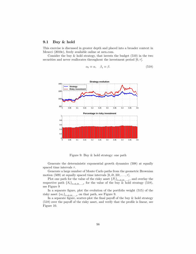
9.1 Buy & hold
This exercise is discussed in greater depth and placed into a broader context inMeucci (2010e), freely available online at ssrn.com.Consider the buy & hold strategy, that invests the budget (510) in the two
securities and never reallocates throughout the investment period [0, τ ].
αt ≡ α, βt ≡ β. (518)
0 0.05 0.1 0.15 0.2 0.25 0.3 0.35 0.4 0.45 0.5800
1000
1200
1400
valu
e
investment (blue) vs underlying (red) value
0 0.05 0.1 0.15 0.2 0.25 0.3 0.35 0.4 0.45 0.50
0.2
0.4
0.6
0.8
1
time
%
percentage of underlying in portfolio
Strategy evolution
Percentage in risky investment
StrategyRisky investment
Figure 9: Buy & hold strategy: one path
Generate the deterministic exponential growth dynamics (508) at equallyspaced time intervals τ .Generate a large number of Monte Carlo paths from the geometric Brownian
motion (509) at equally spaced time intervals [0, δt, 2δt, . . . , τ ].Plot one path for the value of the risky asset {Pt}t=0,δt,...,τ , and overlay the
respective path {St}t=0,δt,...,τ for the value of the buy & hold strategy (518),see Figure 9In a separate figure, plot the evolution of the portfolio weight (515) of the
risky asset {wt}t=0,δt,...,τ on that path, see Figure 9.In a separate figure, scatter-plot the final payoff of the buy & hold strategy
(518) over the payoff of the risky asset, and verify that the profile is linear, seeFigure 10.
98
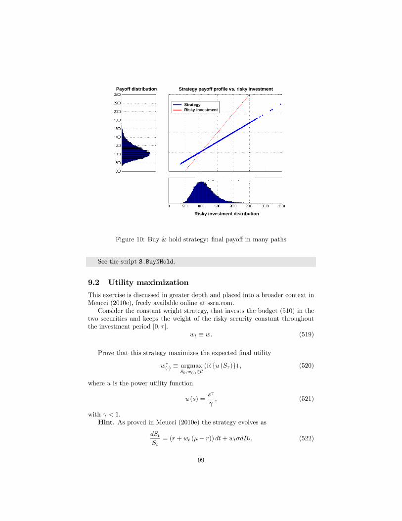
Payoff distribution
Risky investment distribution
StrategyRisky investment
Strategy payoff profile vs. risky investment
Figure 10: Buy & hold strategy: final payoff in many paths
See the script S_BuyNHold.
9.2 Utility maximization
This exercise is discussed in greater depth and placed into a broader context inMeucci (2010e), freely available online at ssrn.com.Consider the constant weight strategy, that invests the budget (510) in the
two securities and keeps the weight of the risky security constant throughoutthe investment period [0, τ ].
wt ≡ w. (519)
Prove that this strategy maximizes the expected final utility
w∗(·) ≡ argmaxS0,w(·)∈C
(E {u (Sτ )}) , (520)
where u is the power utility function
u (s) =sγ
γ, (521)
with γ < 1.Hint. As proved in Meucci (2010e) the strategy evolves as
dStSt
= (r + wt (µ− r)) dt+ wtσdBt. (522)
99
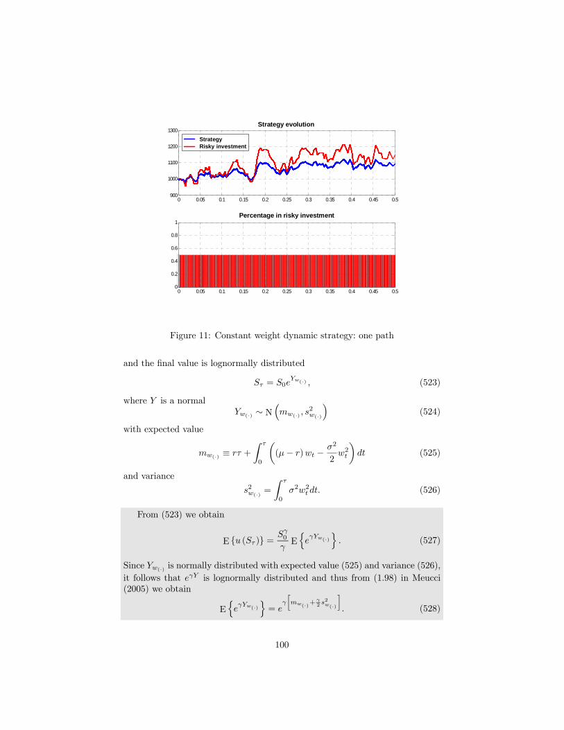
0 0.05 0.1 0.15 0.2 0.25 0.3 0.35 0.4 0.45 0.5900
1000
1100
1200
1300
valu
e
investment (blue) vs underlying (red) value
0 0.05 0.1 0.15 0.2 0.25 0.3 0.35 0.4 0.45 0.50
0.2
0.4
0.6
0.8
1
time
%
percentage of underlying in portfolio
Strategy evolution
Percentage in risky investment
StrategyRisky investment
Figure 11: Constant weight dynamic strategy: one path
and the final value is lognormally distributed
Sτ = S0eYw(·) , (523)
where Y is a normalYw(·) ∼ N
³mw(·) , s
2w(·)
´(524)
with expected value
mw(·) ≡ rτ +
Z τ
0
µ(µ− r)wt −
σ2
2w2t
¶dt (525)
and variance
s2w(·) =
Z τ
0
σ2w2t dt. (526)
From (523) we obtain
E {u (Sτ )} =Sγ0γEneγYw(·)
o. (527)
Since Yw(·) is normally distributed with expected value (525) and variance (526),it follows that eγY is lognormally distributed and thus from (1.98) in Meucci(2005) we obtain
EneγYw(·)
o= e
γ mw(·)+γ2 s
2w(·) . (528)
100
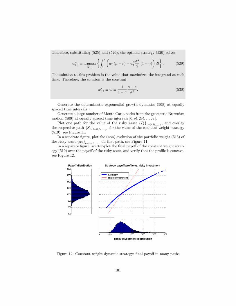
Therefore, substituting (525) and (526), the optimal strategy (520) solves
w∗(·) ≡ argmaxw(·)
½Z τ
0
µwt (µ− r)− w2t
σ2
2(1− γ)
¶dt
¾. (529)
The solution to this problem is the value that maximizes the integrand at eachtime. Therefore, the solution is the constant
w∗(·) ≡ w ≡ 1
1− γ
µ− r
σ2. (530)
Generate the deterministic exponential growth dynamics (508) at equallyspaced time intervals τ .Generate a large number of Monte Carlo paths from the geometric Brownian
motion (509) at equally spaced time intervals [0, δt, 2δt, . . . , τ ].Plot one path for the value of the risky asset {Pt}t=0,δt,...,τ , and overlay
the respective path {St}t=0,δt,...,τ for the value of the constant weight strategy(519), see Figure 11.In a separate figure, plot the (non) evolution of the portfolio weight (515) of
the risky asset {wt}t=0,δt,...,τ on that path, see Figure 11.In a separate figure, scatter-plot the final payoff of the constant weight strat-
egy (519) over the payoff of the risky asset, and verify that the profile is concave,see Figure 12.
Payoff distribution
Risky investment distribution
StrategyRisky investment
Strategy payoff profile vs. risky investment
Figure 12: Constant weight dynamic strategy: final payoff in many paths
101
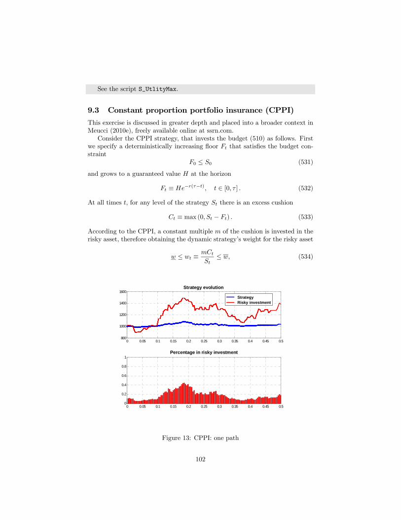
See the script S_UtlityMax.
9.3 Constant proportion portfolio insurance (CPPI)
This exercise is discussed in greater depth and placed into a broader context inMeucci (2010e), freely available online at ssrn.com.Consider the CPPI strategy, that invests the budget (510) as follows. First
we specify a deterministically increasing floor Ft that satisfies the budget con-straint
F0 ≤ S0 (531)
and grows to a guaranteed value H at the horizon
Ft ≡ He−r(τ−t), t ∈ [0, τ ] . (532)
At all times t, for any level of the strategy St there is an excess cushion
Ct ≡ max (0, St − Ft) . (533)
According to the CPPI, a constant multiple m of the cushion is invested in therisky asset, therefore obtaining the dynamic strategy’s weight for the risky asset
w ≤ wt ≡mCt
St≤ w, (534)
0 0.05 0.1 0.15 0.2 0.25 0.3 0.35 0.4 0.45 0.5800
1000
1200
1400
1600
valu
e
investment (blue) vs underlying (red) value
0 0.05 0.1 0.15 0.2 0.25 0.3 0.35 0.4 0.45 0.50
0.2
0.4
0.6
0.8
1
time
%
percentage of underlying in portfolio
Strategy evolution
Percentage in risky investment
StrategyRisky investment
Figure 13: CPPI: one path
102
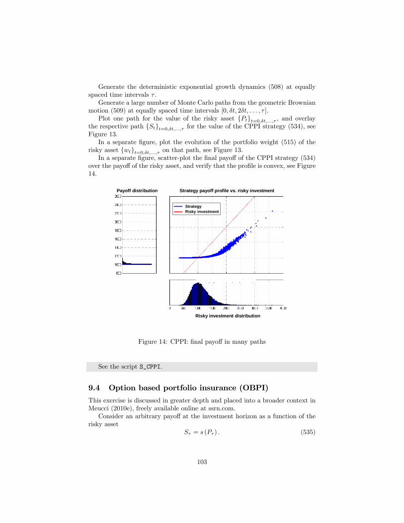
Generate the deterministic exponential growth dynamics (508) at equallyspaced time intervals τ .Generate a large number of Monte Carlo paths from the geometric Brownian
motion (509) at equally spaced time intervals [0, δt, 2δt, . . . , τ ].Plot one path for the value of the risky asset {Pt}t=0,δt,...,τ , and overlay
the respective path {St}t=0,δt,...,τ for the value of the CPPI strategy (534), seeFigure 13.In a separate figure, plot the evolution of the portfolio weight (515) of the
risky asset {wt}t=0,δt,...,τ on that path, see Figure 13.In a separate figure, scatter-plot the final payoff of the CPPI strategy (534)
over the payoff of the risky asset, and verify that the profile is convex, see Figure14.
Payoff distribution
Risky investment distribution
StrategyRisky investment
Strategy payoff profile vs. risky investment
Figure 14: CPPI: final payoff in many paths
See the script S_CPPI.
9.4 Option based portfolio insurance (OBPI)
This exercise is discussed in greater depth and placed into a broader context inMeucci (2010e), freely available online at ssrn.com.Consider an arbitrary payoff at the investment horizon as a function of the
risky assetSτ = s (Pτ ) . (535)
103
and assume that you can compute the solution G (t, p) of the following partialdifferential equation
∂G
∂t+
∂G
∂pr +
1
2
∂2G
∂p2σ2p2 −Gr = 0, (536)
with boundary condition
G (τ , p) ≡ s (p) , p > 0, (537)
Prove that a strategy that invests an initial budget
S0 ≡ G (0, P0) (538)
and allocates dynamically the following weight in the risky asset
wt ≡PtSt
∂G (t, Pt)
∂Pt, (539)
provides the desired payoff (535).Hint. As proved in Meucci (2010e) the strategy evolves as
dStSt
= (r + wt (µ− r)) dt+ wtσdBt. (540)
We want to prove that the following identity holds at all times, and inparticular at t ≡ τ
St ≡ G (t, Pt) , t ∈ [0, τ ] . (541)
Indeed, using Ito’s rule on G (t, Pt), where Pt follows the geometric Brownianmotion (509) yields
dGt =∂G
∂tdt+
∂G
∂PtdPt +
1
2
∂2G
∂P 2t(dPt)
2
=∂G
∂tdt+
∂G
∂Pt(µPtdt+ σPtdB) +
1
2
∂2G
∂P 2tσ2P 2t dt (542)
=
µ∂G
∂t+
∂G
∂PtµPt +
1
2
∂2G
∂P 2tσ2P 2t
¶dt+
∂G
∂PtσPtdBt.
Also, from (540) and (539) we obtain
dSt = Strdt+ Stwt
µdPtPt− rdt
¶= Strdt+ Pt
∂G
∂Pt
µdPtPt− rdt
¶(543)
= Strdt+∂G
∂Pt(µPtdt+ σPtdBt − Ptrdt)
104
Therefore
d (Gt − St) =
µ∂G
∂t+
∂G
∂PtµPt +
1
2
∂2G
∂P 2tσ2P 2t
¶dt+
∂G
∂PtσPtdBt
−Strdt−∂G
∂Pt(µPtdt+ σPtdBt − Ptrdt) (544)
=
µ∂G
∂t+1
2
∂2G
∂P 2tσ2P 2t − Str +
∂G
∂PtPtr
¶dt
Using (536) we finally obtain
d (Gt − St)
(Gt − St)= rdt, (545)
Which means(Gτ − Sτ ) = (G0 − S0) e
rτ . (546)
Since from (538) we have G0 − S0 = 0, it follows that (541) holds true.
Assume that the payoff (535) is that of a call option with strike K
s (p) ≡ max (0, p−K)
In this context the partial differential equation (536) was solved in Black andScholes (1973)
G (t, p) = pΦ (d1)− e−r(τ−t)KΦ (d2) , (547)
where Φ is the cumulative distribution for the standard normal distribution and
d1 (t, p) ≡1
σ√τ − t
µln³ p
K
´+
µr +
σ2
2
¶(τ − t)
¶(548)
d2 (t, p) ≡ d1 (t, p)− σ√τ − t. (549)
From the explicit analytical expression (547) we can derive the expression forthe weight (539) of the risky asset
wt =PtStΦ (d1 (t, Pt)) . (550)
Generate the deterministic exponential growth dynamics (508) at equallyspaced time intervals τ .Generate a large number of Monte Carlo paths from the geometric Brownian
motion (509) at equally spaced time intervals [0, δt, 2δt, . . . , τ ].Plot one path for the value of the risky asset {Pt}t=0,δt,...,τ , and overlay the
respective path {St}t=0,δt,...,τ for the value of the option replication strategy(550), see Figure 15.In a separate figure, plot the evolution of the portfolio weight of the risky
asset {wt}t=0,δt,...,τ on that path, see Figure 15.
105
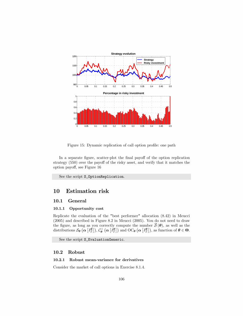
0 0.05 0.1 0.15 0.2 0.25 0.3 0.35 0.4 0.45 0.5900
1000
1100
1200
valu
e
investment (blue) vs underlying (red) value
0 0.05 0.1 0.15 0.2 0.25 0.3 0.35 0.4 0.45 0.50
0.2
0.4
0.6
0.8
1
time
%
percentage of underlying in portfolio
Strategy evolution
Percentage in risky investment
StrategyRisky investment
Figure 15: Dynamic replication of call option profile: one path
In a separate figure, scatter-plot the final payoff of the option replicationstrategy (550) over the payoff of the risky asset, and verify that it matches theoption payoff, see Figure 16
See the script S_OptionReplication.
10 Estimation risk
10.1 General
10.1.1 Opportunity cost
Replicate the evaluation of the "best performer" allocation (8.42) in Meucci(2005) and described in Figure 8.2 in Meucci (2005). You do not need to drawthe figure, as long as you correctly compute the number S (θ), as well as thedistributions Sθ
¡α£IθT¤¢, C+θ
¡α£IθT¤¢and OCθ
¡α£IθT¤¢, as function of θ ∈Θ.
See the script S_EvaluationGeneric.
10.2 Robust
10.2.1 Robust mean-variance for derivatives
Consider the market of call options in Exercise 8.1.4.
106
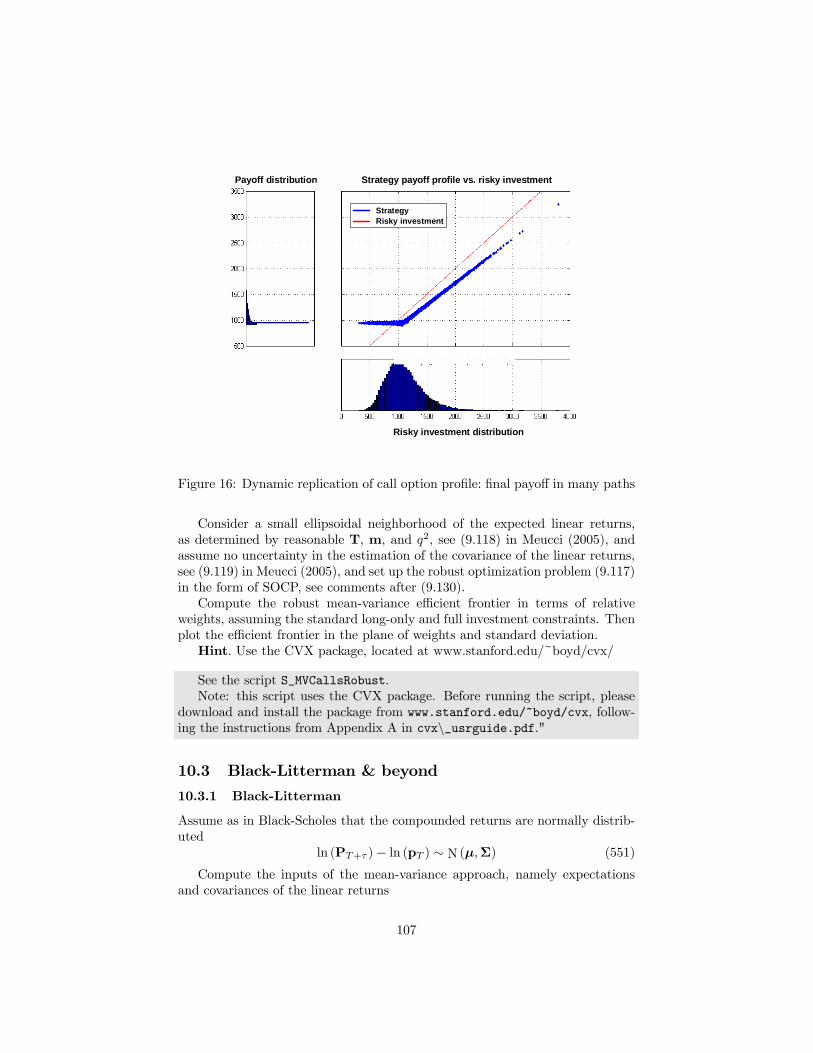
Strategy payoff profile vs. risky investmentPayoff distribution
Risky investment distribution
StrategyRisky investment
Figure 16: Dynamic replication of call option profile: final payoff in many paths
Consider a small ellipsoidal neighborhood of the expected linear returns,as determined by reasonable T, m, and q2, see (9.118) in Meucci (2005), andassume no uncertainty in the estimation of the covariance of the linear returns,see (9.119) in Meucci (2005), and set up the robust optimization problem (9.117)in the form of SOCP, see comments after (9.130).Compute the robust mean-variance efficient frontier in terms of relative
weights, assuming the standard long-only and full investment constraints. Thenplot the efficient frontier in the plane of weights and standard deviation.Hint. Use the CVX package, located at www.stanford.edu/~boyd/cvx/
See the script S_MVCallsRobust.Note: this script uses the CVX package. Before running the script, please
download and install the package from www.stanford.edu/~boyd/cvx, follow-ing the instructions from Appendix A in cvx\_usrguide.pdf."
10.3 Black-Litterman & beyond
10.3.1 Black-Litterman
Assume as in Black-Scholes that the compounded returns are normally distrib-uted
ln (PT+τ )− ln (pT ) ∼ N(µ,Σ) (551)
Compute the inputs of the mean-variance approach, namely expectationsand covariances of the linear returns
107
Also from (2.219)-(2.220) in Meucci (2005) for a log-normal variable
Y ∼ LogN (µ,Σ) . (552)
then
E {Y} = eµ+12 diag(Σ). (553)
E©YY0ª =
³e(µ+
12 diag(Σ))e(µ+
12 diag(Σ))0
´◦ eΣ, (554)
where ◦ denotes the term-by-term Hadamard product.Since
1 +R ∼ LogN (µ,Σ) , (555)
using (361), (362) and the property
E {(Y − 1)} = E {Y}− 1 (556)
E©(Y − 1) (Y − 1)0
ª= E
©YY0ª+ 110 − E©Y10ª− E©1Y0ª . (557)
we can easily compute the expectations E {R} and the second momentsE©RR0ª. The covariance then follows from
Cov {R} = E©RR0ª− E {R}E {R0} . (558)
Upload the database CovNRets that contains estimates for µ and Σ. Usethe results from the previous point to compute and plot numerically the efficientfrontier under the constraints that the weights sum to one and that they arenon-negative.Construct a pick matrix that sets views on the spread between the com-
pounded return of the first and the last security. Set a one-standard deviationbullish view on that spread. Use the market-based Black-Litterman formula(9.44) in Meucci (2005) to compute the normal parameters that reflect thoseviews. Map the results into expectations and covariances for the linear returns.Compute and plot numerically the efficient frontier under the same constraintsas above
See script S_BLmBasic.
10.3.2 Beyond Black-Litterman
Consider the market prior
Xd= BZ−1 + (1−B)Z1 (559)
whereZ−1 ∼ N(−1, 1) , Z1 ∼ N(1, 1) ; (560)
108

B is Bernoulli with P {B = 1} ≡ 1/2; and all the variables are independent.Compute and plot the posterior market distribution that is the most consis-
tent with the view eE {X} ≡ 0.5. (561)
Hint. Use the package "Entropy Pooling: Fully Flexible Views and Stress-testing" available at www.mathworks.com/matlabcentral/fileexchange/21307.
See script S_EntropyView.
109

ReferencesBlack, F., and M. S. Scholes, 1973, The pricing of options and corporate liabil-ities, Journal of Political Economy 81, 637—654.
Kendall, M.G., and A. Stuart, 1969, The Advanced Theory of Statistics, Volume(Griffin) third edn.
Meucci, A., 2005, Risk and Asset Allocation (Springer).
, 2009a, Review of discrete and continuous processes in fi-nance: Theory and applications, Working paper Available athttp://ssrn.com/abstract=1373102.
, 2009b, Review of statistical arbitrage, cointegration, andmultivariate Ornstein-Uhlenbeck, Working Paper Available athttp://ssrn.com/abstract=1404905.
, 2009c, Simulations with exact means and covariances, Risk 22, 89—91Extended version available at http://ssrn.com/abstract=1415699.
, 2010a, Annualization and general projection of skweness, kur-tosis, and all summary statistics, GARP Risk Professional - "TheQuant Classroom" August, 55—56 Available as "Quant Nugget 4" athttp://ssrn.com/abstract=1635484.
, 2010b, Common misconceptions about ’beta’ - hedging, estimation andhorizon effects, GARP Risk Professional - "The Quant Classroom" June, 42—45 Available as "Quant Nugget 3" at http://ssrn.com/abstract=1619923.
, 2010c, Factors on Demand - building a platform for portfo-lio managers risk managers and traders, Risk 23, 84—89 Available athttp://ssrn.com/abstract=1565134.
, 2010d, Linear vs. compounded returns - common pitfalls in portfoliomanagement, GARP Risk Professional - "The Quant Classroom" April, 52—54 Available as "Quant Nugget 2" at http://ssrn.com/abstract=1586656.
, 2010e, Review of dynamic allocation strategies: Con-vex versus concave management, Working Paper Available athttp://ssrn.com/abstract=1635982.
, 2010f, Review of linear factor models: Unexpected common fea-tures and the systematic-plus-idiosyncratic myth, Working paper Availableat http://ssrn.com/abstract=1635495.
, 2010g, Square-root rule, covariances and ellipsoids - how to an-alyze and visualize the propagation of risk, GARP Risk Professional -"The Quant Classroom" February, 52—53 Available as "Quant Nugget 1" athttp://ssrn.com/abstract=1548162.
110

Petkov, P. H., N. D. Christov, and M. M. Konstantinov, 1991, ComputationalMethods for Linear Control Systems (Prentice Hall).
111