Exercise 1:

Introduction to QGIS

Aim: • To understand the basis of GIS

• To learn the basics of a GIS software (QGIS)

INTRODUCTION

Software Access Download the Latest LTR QGIS version (2.18) from the QGIS website: download.qgis.org/

Data Access

Download the data of the Exercise 1 from the course website.

EXERCISE

Getting Started

Open QGIS. If the window language is not English, go to

>> Settings > Options > Locale …

And set the language to US English. Restart QGIS. We will first load a background map to our project. To do so, we will use the Openlayers plug-in. If it is the first time you use QGIS, it is likely that you don’t have this plug-in installed yet. To download and install a plug-in go to:

>> Plugins > Manage and Intall Plugins…

Search for ‘Openlayers Plugin’, click on Install Plugin and make sur that the box next the name is ticked. Close the plugins window. Note: Use the Plugin Manager to retrieve any the plugins you need during the exercise. To load the OpenStreetMap background map go to:

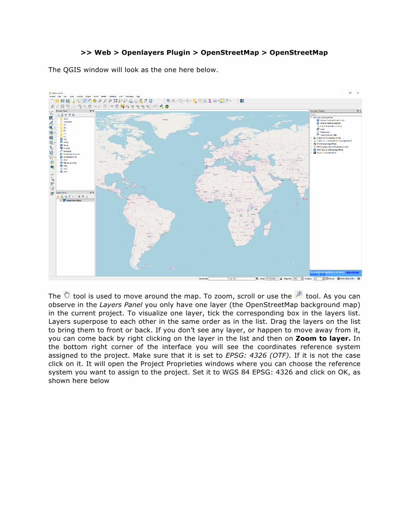
>> Web > Openlayers Plugin > OpenStreetMap > OpenStreetMap The QGIS window will look as the one here below.

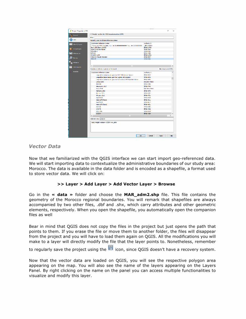
The tool is used to move around the map. To zoom, scroll or use the tool. As you can observe in the Layers Panel you only have one layer (the OpenStreetMap background map) in the current project. To visualize one layer, tick the corresponding box in the layers list. Layers superpose to each other in the same order as in the list. Drag the layers on the list to bring them to front or back. If you don’t see any layer, or happen to move away from it, you can come back by right clicking on the layer in the list and then on Zoom to layer. In the bottom right corner of the interface you will see the coordinates reference system assigned to the project. Make sure that it is set to EPSG: 4326 (OTF). If it is not the case click on it. It will open the Project Proprieties windows where you can choose the reference system you want to assign to the project. Set it to WGS 84 EPSG: 4326 and click on OK, as shown here below

Vector Data Now that we familiarized with the QGIS interface we can start import geo-referenced data. We will start importing data to contextualize the administrative boundaries of our study area: Morocco. The data is available in the data folder and is encoded as a shapefile, a format used to store vector data. We will click on:

>> Layer > Add Layer > Add Vector Layer > Browse

Go in the « data » folder and choose the MAR_adm2.shp file. This file contains the geometry of the Morocco regional boundaries. You will remark that shapefiles are always accompanied by two other files, .dbf and .shx, which carry attributes and other geometric elements, respectively. When you open the shapefile, you automatically open the companion files as well

Bear in mind that QGIS does not copy the files in the project but just opens the path that points to them. If you erase the file or move them to another folder, the files will disappear from the project and you will have to load them again on QGIS. All the modifications you will make to a layer will directly modify the file that the layer points to. Nonetheless, remember

to regularly save the project using the icon, since QGIS doesn’t have a recovery system. Now that the vector data are loaded on QGIS, you will see the respective polygon area appearing on the map. You will also see the name of the layers appearing on the Layers Panel. By right clicking on the name on the panel you can access multiple functionalities to visualize and modify this layer.

Every vector layer carries an attribute table with information about each of the objects. Bring the MAR_adm2.shp layer in front and right click on the layer list and choose Open Attribute Table. Each line corresponds to a different object. You can select an object by clicking on its row and it will appear in yellow in the map. You can also go the other way round by using the tool in the map and selecting an object. It will appear highlighted in the attribute table. Use crtl (cmd on mac) while clicking to choose multiple objects. Q1. What do the different columns correspond to? The objects appear all in the same color and it is therefore hard to make distinctions. You can fix this by right clicking on the layer in the list and choosing Properties > Style. You can modify the style from Single Symbol to Categorized. Here you can choose a column from the attribute table to use to distinguish the objects. In our case, the ID_1 distinguish different type of regions. Choose it and click on Classify, then Apply and OK.

If you want to access the attribute of an object without opening the attribute table, you can use the tool (remember to select the layer you want to investigate in the Layers Panel. Import Environmental Data Now that we have contextualized our study area we want to characterize the landscape. To do so, we will start observing two variables: altitude and temperature. This data is stored as a raster file in the geotiff format. To open it, click on:

>> Layer > Add Layer > Add Raster Layer And choose DEM.gtiff and MYT.gtiff. The first file corresponds to a Digital Elevation Model, the second one to the Mean Yearly Temperature. The two layers will appear in a greyscale. To better visualize the value on the map, we will change the color scales. To do so, right click on the raster layer you want to modify in the Layers Panel:

>> Properties > Style

Switch render type to Singleband Pseudocolor, ad choose a colorscale you want to apply to the data (for ex. YlOrRd). Click on classify and then on ok. For example, the temperature map will look as the one here below.

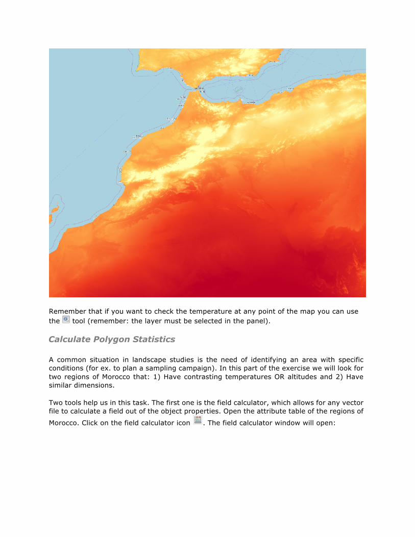
Remember that if you want to check the temperature at any point of the map you can use the tool (remember: the layer must be selected in the panel). Calculate Polygon Statistics A common situation in landscape studies is the need of identifying an area with specific conditions (for ex. to plan a sampling campaign). In this part of the exercise we will look for two regions of Morocco that: 1) Have contrasting temperatures OR altitudes and 2) Have similar dimensions. Two tools help us in this task. The first one is the field calculator, which allows for any vector file to calculate a field out of the object properties. Open the attribute table of the regions of

Morocco. Click on the field calculator icon . The field calculator window will open:

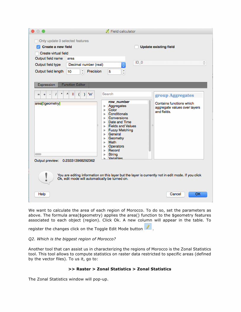
We want to calculate the area of each region of Morocco. To do so, set the parameters as above. The formula area($geometry) applies the area() function to the $geometry features associated to each object (region). Click Ok. A new column will appear in the table. To

register the changes click on the Toggle Edit Mode button . Q2. Which is the biggest region of Morocco? Another tool that can assist us in characterizing the regions of Morocco is the Zonal Statistics tool. This tool allows to compute statistics on raster data restricted to specific areas (defined by the vector files). To us it, go to:

>> Raster > Zonal Statistics > Zonal Statistics The Zonal Statistics window will pop-up.

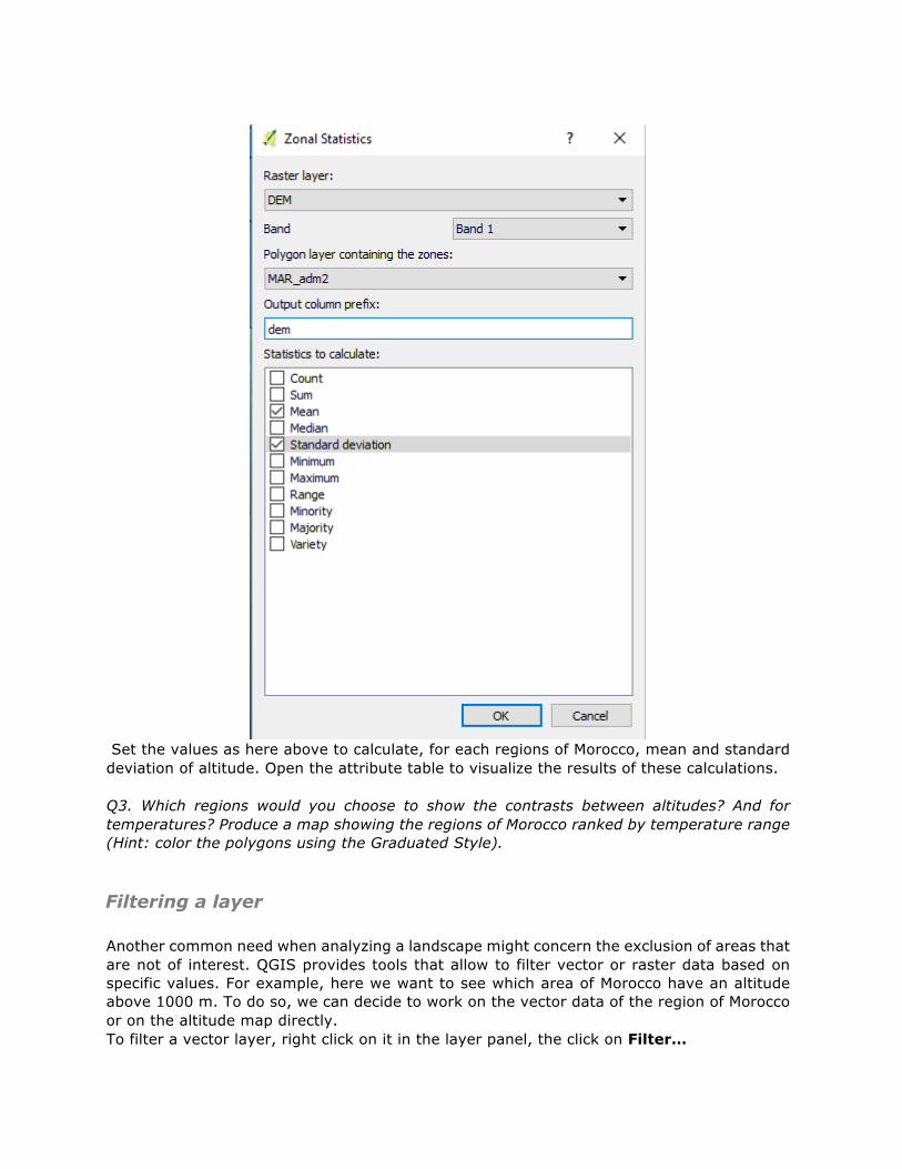
Set the values as here above to calculate, for each regions of Morocco, mean and standard deviation of altitude. Open the attribute table to visualize the results of these calculations. Q3. Which regions would you choose to show the contrasts between altitudes? And for temperatures? Produce a map showing the regions of Morocco ranked by temperature range (Hint: color the polygons using the Graduated Style). Filtering a layer Another common need when analyzing a landscape might concern the exclusion of areas that are not of interest. QGIS provides tools that allow to filter vector or raster data based on specific values. For example, here we want to see which area of Morocco have an altitude above 1000 m. To do so, we can decide to work on the vector data of the region of Morocco or on the altitude map directly. To filter a vector layer, right click on it in the layer panel, the click on Filter…

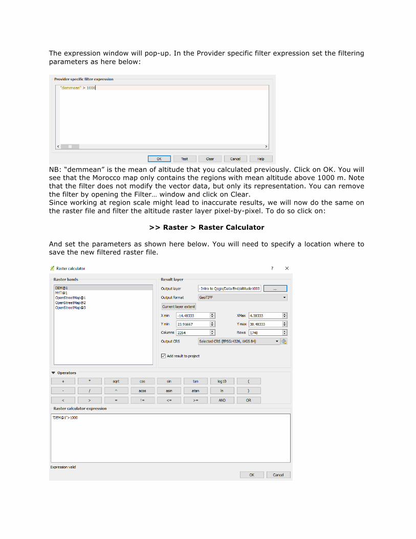
The expression window will pop-up. In the Provider specific filter expression set the filtering parameters as here below:

NB: “demmean” is the mean of altitude that you calculated previously. Click on OK. You will see that the Morocco map only contains the regions with mean altitude above 1000 m. Note that the filter does not modify the vector data, but only its representation. You can remove the filter by opening the Filter… window and click on Clear. Since working at region scale might lead to inaccurate results, we will now do the same on the raster file and filter the altitude raster layer pixel-by-pixel. To do so click on:

>> Raster > Raster Calculator

And set the parameters as shown here below. You will need to specify a location where to save the new filtered raster file.

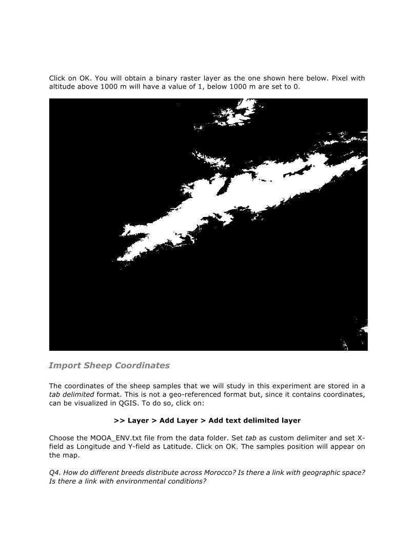
Click on OK. You will obtain a binary raster layer as the one shown here below. Pixel with altitude above 1000 m will have a value of 1, below 1000 m are set to 0.

Import Sheep Coordinates The coordinates of the sheep samples that we will study in this experiment are stored in a tab delimited format. This is not a geo-referenced format but, since it contains coordinates, can be visualized in QGIS. To do so, click on:

>> Layer > Add Layer > Add text delimited layer Choose the MOOA_ENV.txt file from the data folder. Set tab as custom delimiter and set X-field as Longitude and Y-field as Latitude. Click on OK. The samples position will appear on the map. Q4. How do different breeds distribute across Morocco? Is there a link with geographic space? Is there a link with environmental conditions?

Right click on the MOOA_ENV layer and the click on Save as… to register it as a shapefile.