exchange rate regimes and inflation: evidence from india biswajit
TRANSCRIPT
Exchange Rate Regimes and Inflation: Evidence from India Biswajit Mohanty and N R Bhanumurthy
Working Paper No. 2014-130
February 2014
National Institute of Public Finance and Policy
New Delhi
http://www.nipfp.org.in
2
Exchange Rate Regimes and Inflation: Evidence from India
Biswajit Mohantya
and
N R Bhanumurthyb
Abstract
Exchange rate stability is crucial for inflation management as a stable rate is
expected to reduce domestic inflation pressures through a ‘policy discipline effect’- restricting money supply growth, and a ‘credibility effect’- inducing higher money demand and reduced velocity of money. Alternatively, the impossibility trillema predicts that in the presence of an open capital account, a stable exchange rate may lead to lack of control on monetary policy and, hence, higher inflation. Using a monetary model of Inflation, this paper investigates the impact of the de facto stable exchange rate regime on inflation in India during different episodes of exchange rate stability. The results show that the impact of exchange rate regime on inflation is not visible in Indian case, which could be because of the offsetting sterilization policy undertaken by Reserve Bank of India (RBI) during expansionary money supply growth resulting from its large scale intervention to even out exchange rate volatility. Key words: Exchange rate regime; Inflation; Money supply; ARDL Model, India JEL classification: E52; F33; F41
a UGC Research Scholar, Department of Business Economics, Delhi University, New Delhi, India.
E-mail: [email protected] b Professor, National Institute of Public Finance and Policy, New Delhi, India. E-Mail:
3
Introduction
Ever since the collapse of Bretton Woods’s system, the choice of exchange rate
regime, particularly in developing and emerging economies, has been assessed frequently. More so, during the early 1990s, several economies that were in transition from controlled to market economies, including those in Asia, and had soft (and also crawling) peg regimes, experienced collapse of their currencies due to sharp reversal of capital flows leading to the Asian crisis of 1997. In addition, skepticism about the credibility of intermediate exchange rate regime led to widely accepted ‘bipolar view’ or ‘corner solution’, i.e., a country should either adopt hard pegs (monetary union or currency boards) or free floats. But, hard peg solution became out of favor with the collapse of Argentina’s currency board resulting in Argentinean crisis of 2002. Accordingly, majority of the emerging and developing countries have gone for more flexible exchange rate regimes. However, this regime shift has not witnessed a pure float. Rather, adopted a ‘constrained floating’ since monetary authorities in these countries may be affected by a ‘fear of float’. Calvo and Reinhart (2002) observe that official or de jure exchange rate regime as reported by countries’ monetary authorities may be different from the actual or de facto exchange rate regime based on the actual behavior of the exchange rates. Most of the countries announcing a floating regime have an underlying ‘fear of floating’ and hence, may intervene regularly on the foreign exchange market resulting in a de facto fixed regime. This preference for exchange rate stability is, particularly, prevalent in developing and emerging economies for which sharp appreciation or depreciation of the currencies is more harmful as they do not have the institutional requirements for undertaking effective monetary policy under purely floating exchange rates (Summers(2000)).
How to evaluate exchange rate regimes? In the literature, the episodes of high inflation in many countries at the end of the 1970s and during 1980s led to focus on the credibility aspects of exchange rate regime and whether they can be used to achieve low inflation rates. Riddled with conflicting view points and counter arguments, broadly, the theoretical literature favors exchange rate stability for inflation consequences; but with more capital account openness, the stable regime can also be considered inflationary due to the existence of ‘impossibility trillema’ of Mundell (1961). Moreover, the empirical findings ranges from stable regime –lower inflation association to its opposite and even regime neutrality of inflation.
India has gone through several regime shifts overtime – a par value system of International Monetary Fund (IMF) during 1950s, a basket peg during 1970s and 1980s and finally a market determined exchange rate between March 1992 and February 1993 [Patnaik, et al. (2003)]. RBI’s official position after 1993 is that the exchange rate policy focuses on ‘managing volatility’ with no fixed target, while allowing the underlying demand and supply conditions to determine exchange rate movements in an orderly way (RBI, 1993). Thus even though it is market determined, the exchange rate regime is not a pure float but a managed float with no preannounced paths. Though most of the official pronouncements identify the exchange rate regime since 1993 as managed float including the IMF and RBI, there is a controversy surrounding the issue of whether the de facto regime of India has changed to a managed float. Studies examining the behavior of India’s de facto regime has observed it to be a peg to US dollar since it exhibits very low
4
and unchanged flexibility since 1979 [ Calvo & Reinhart(2002), Reinhart & Rogoff( 2004), Patnaik(2003)].
Given the de facto stability of India’s exchange rate regime, this paper tries to examine the hypothesis that whether a stable exchange rate regime leads to lower inflation. While a few earlier studies such as Patel & Srivastava (1998) have examined the consequences of real exchange rate targeting for inflation in terms of exchange rate `pass through' into domestic inflation, studies such as Patnaik (2004) and Hutchison et al., (2012) have dealt with the implication of India’s de facto pegged regime for monetary policy independence. Even though these studies focused on ‘impossible trinity’ to explain the exchange rate regime-inflation link, they have not comprehensive in terms of theoretical channels of regime-inflation link. Unlike the earlier studies, this study looks into the direct and indirect channels -such as credibility effect of the exchange rate regime visible through its impact on interest rate and velocity of money; and disciplined effect working on money supply, through which exchange rate regime may ultimately influence inflation. Further, the existing studies do not consider the issue of endogeneity or reverse causation, which implies bi-directional causality between exchange rate regime and inflation. Ignoring endogeneity might give a misleading result of the impact of regime on inflation. Our study addresses this issue to attain robust results. Further, we examine the regime-inflation relationship in different periods in terms of the extent of exchange rate stability and also in the long run and short run, which makes the analysis more comprehensive.
The paper is organized as follows. Section 2 briefly reviews the empirical literature on exchange rate regime and inflation link. Section 3 presents the empirical model and methodology adopted in the study. Section 4 describes the data and variables. Section 5 offers the analysis of India’s exchange rate regime. Section 6 reports the empirical results and findings and Section 7 concludes.
2. Exchange Rate Regime and Inflation: Theoretical Overview
Following Barro and Gordon (1983) on monetary policy credibility, some more studies [Velasco (1996), Benigno and Missale (2004), Giavazzi and Giovannini (1989) and Dornbusch (2001)] developed the idea that a fixed or stable exchange rate policy could help impart credibility of low inflation policies of a central bank. The main argument in favor of stable exchange rate regimes is the ability of such regimes to induce price discipline and commitment to monetary policy efficiency. Under a fixed or stable exchange rate system, a nation with a higher rate of inflation than the rest of the world is likely to face persistent deficits in its balance of payments resulting in loss of reserves. Due to the unsustainability of the persistent deficits and reserve losses, the nation needs to restrain its excessive rate of inflation and, thus, faces some price discipline. But, under flexible exchange rate system, there is no such pressure for price discipline, where balance of payments disequilibria are automatically and instantaneously corrected by changes in the exchange rate. In this view, the exchange rate represents a “nominal anchor” for monetary policy (Bernanke, et.al 1999).
Another argument is that a fixed exchange rate will increase credibility so that the central bank’s announcements about its commitment to low inflation are believed,
5
thus providing an anchor for expectations of inflation, which may happen through wage contracts, become self-fulfilling and result in lower inflation. This reduced inflationary expectation could curb money velocity and reduce the sensitivity of prices to temporary monetary shocks (Levy-Yeyati & Sturzenegger, (2000)). In addition, pegging the exchange rate can also lower inflation by producing a “confidence effect,” i.e. a greater willingness to hold domestic currency rather than goods or foreign currencies (Ghosh et al (1997)). Further, the arguments against fluctuating exchange rates are that they are associated with overshooting of the equilibrium exchange rate in both directions and cause prices to rise by raising the domestic prices of imported final and intermediate goods when depreciating but fail to reduce prices while appreciating (the so called ratchet effect). Thus, inflation is likely to be higher under a flexible than a fixed exchange rate system.
Against the claim that fixed rates induce more discipline, Tornell & Velasco (1994) argue that a flexible rate allow the effect of unsound fiscal policies to be reflected in exchange rate movements and given that inflation is costly for fiscal authorities, the flexible rates enforce transparency and provide more policy discipline by forcing them to pay the cost. It is also argued that flexible regime provides monetary independence, which, in turn, is crucial for tracking the monetary policy in direction that stimulates growth and reduces unemployment. In terms of its impact on growth, monetary independence with exchange rate floating will ensure the government to focus on optimal inflation rate that is beneficial for the growth of the economy (Hernandez-Verme (2004)). On balance, the above theoretical arguments seem to provide divergent views on the role the exchange rate regimes have on inflation management.
Empirical studies on exchange rate regimes and inflation have also appeared to have shown mixed findings. While a number of empirical studies found that various forms of fixed exchange rates indeed lower inflation, other studies found the exchange rate to be an ineffective nominal anchor. The findings of Ghosh et al (1997, 2003) suggests that pegging the nominal exchange rate is associated with lower inflation because of reduced monetary growth, lower residual velocity growth controlling for income and interest rate. Similar results follow from the findings of Levy-Yeyati & Sturzenegger (2000) and Bleaney& Francisco (2007) which confirm the theoretical viewpoint of negative relationship between pegged regime and inflation and further, that pegged and intermediate regime are on average less inflationary than float
1. Other studies like Miles
(2008), De grauwe & Schnabl (2004), Domac et al (2001), and Garofalo (2005) could not find any significant relationship between exchange rate regime and inflation.
These conflicting results across studies could be due to classification of exchange rate regime (de facto or de jure), the problem of endogeneity of exchange rate regime and more importantly, most studies are based on cross-country cases that may not account for underlying country specific factors. The problem of endogeneity of the exchange rate regime points to a possibility of two-way causality between inflation and exchange rate regime giving rise to a possible bias on the impact of regime on inflation. It is not clear whether fixed exchange rates deliver low inflation by adding discipline and credibility to the conduct of macroeconomic policies or whether countries with low inflation choose pegged exchange rates, perhaps to signal their intention to maintain their anti-inflationary stance, or they have better chances to implement a sustainable peg.
1 In these group of studies, only the long and hard pegs matter for this negative relationship and
that too only in the case of non-industrial or developing countries.
6
Lucas critique postulates that in case of a policy switch the coefficients associated with policy variables should change. For example, the coefficients of policy variables like money supply and nominal interest rate in the inflation equation will be different under different exchange rate regime and as a result, there will be different response of inflation to these policy variables under different exchange rate regimes. It is also important to see how country specific characters would affect the results. In the next section, we look at the India-specific studies on this issue. 2.1 Studies on India
In the case of India, there are very few studies that have discussed the exchange rate regime-inflation relation in terms of impossible trinity where a country cannot have simultaneously a fixed exchange rate, capital mobility and monetary independence. The explanation is that monetary policy in a country with fixed-exchange-rate is imported from the reserve currency country. The monetary policy of the pegging country must ensure that its interest rate are aligned with its partner’s as any interest rate divergence between two such countries will lure speculators being engaged in selling and buying of one currency against the other, which results in foreign capital inflows until interest rates are equalized. If the country tries to keep down the exchange rate through intervention, it will experience increase/decrease in base money and hence, lower/higher interest rates, which renders its attempts to have an independent monetary policy ineffective. Thus, the monetary authority cannot use monetary policy variables like money supply, interest rate to achieve domestic objectives like inflation control [Mundell (1961)]. In India, since the liberalization of the economy in 1991, the process of capital account liberalization has been rather gradual. Though there has been relaxation on capital controls in several forms such as less stringent requirements for and higher limits on foreign institutional investors (FIIs), simplification of approval processes and easy access for FIIs in currency markets, substantial controls on capital inflows continue to exist (Hutchison et al.(2012)).
In spite of the slow process of capital account liberalization, the economy has been witnessing sharp increases in capital inflows over the last decade, especially in the years prior to the recent global financial crisis that started in 2007(Hutchison et al.(2012)). The low exchange rate flexibility and the rising capital inflows are likely to result in distortions in the monetary policy. More so, as the RBI is managing the exchange rate heavily through large scale intervention, it accumulates increasing foreign exchange reserves, resulting in rise in the monetary base. As the rise in monetary base due to accumulation of international reserves has implication on loss of monetary policy autonomy and, hence, inimical for price stability, RBI has to take recourse to sterilization of inflows by ‘selling off government securities (decline in net domestic assets) to maintain monetary control’ (IMF Country Report, Table 4, March 2010).
In the pre-reform period, some studies have found that real exchange rate targeting have not had any impact on inflation and this was largely due to relatively lower inflation in India compared to trading partners (Patel & Srivastava (1998)). But this result may not be robust as there were higher capital inflows in the post-reform period. The studies on post-reform India show that there were indeed episodes of de facto pegged regimes in India and they are found to come at the cost of monetary policy autonomy (Patnaik (2004)). Some have shown that due to increase in capital account openness, atleast in the post-2000s, exchange rate volatility has increased and led to higher inflation while in episodes of exchange rate stability, the inflation volatility turned out to be lower (Hutchison et al., (2012)). Even though these studies rely on ‘impossible trinity’ to explain
7
the regime-inflation link, they do not consider the role of endogeneity or reverse causation, which implies two way causality between exchange rate regime and inflation. Hence, considering only the usual theoretical relation between exchange rate and inflation may not provide complete understanding of regime-inflation relationship.
Based on the above theoretical and empirical literature, we investigate the relationship between exchange rate regime and inflation in India. For this, we frame two alternative hypotheses. One, the stability or low flexibility of exchange rate regime in India is less inflationary, which follows from the general standpoint of superiority of fixed exchange rate regime over a flexible one. Two, the very stability of exchange rate is associated with higher inflation as a result of ‘the impossible trinity’ at work. This study also examines endogenity problem.
3. Empirical Model and Methodology
The typical association of fixed exchange rates with lower inflation rates is based primarily on the belief that a peg may play the role of a commitment mechanism for monetary authorities. This effect works entirely through the behavior of the monetary aggregates. A credible peg also leads to higher money demand and low inflation expectations (which might stabilize money velocity) and reduce the sensitivity of prices with respect to upward changes in money growth. Having these two effects of regime on inflation, i.e., discipline effect and credibility effect, we broadly adopt the monetary model framework used by Ghosh et al (1997).
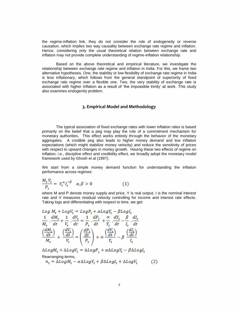
We start from a simple money demand function for understanding the inflation performance across regimes:
where M and P denote money supply and price, Y is real output, I is the nominal interest rate and V measures residual velocity controlling for income and interest rate effects. Taking logs and differentiating with respect to time, we get:
Rearranging terms,
8
Where, π t = Δ Log Pt is inflation rate , Δ Log Mt is broad money growth rate, Δ Log It is growth rate of nominal interest rate, Δ Log
Y t is real output growth rate , Δ Log V t is
growth rate of money velocity.
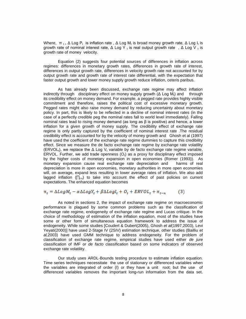
Equation (2) suggests four potential sources of differences in inflation across regimes: differences in monetary growth rates, differences in growth rate of interest, differences in output growth rate, differences in velocity growth rate not accounted for by output growth rate and growth rate of interest rate differential, with the expectation that faster output growth and lower money supply growth reduce inflation, ceteris paribus.
As has already been discussed, exchange rate regime may affect inflation indirectly through disciplinary effect on money supply growth (Δ Log Mt) and through its credibility effect on money demand. For example, a pegged rate provides highly visible commitment and therefore, raises the political cost of excessive monetary growth. Pegged rates might also raise money demand by reducing uncertainty about monetary policy. In part, this is likely to be reflected in a decline of nominal interest rates (in the case of a perfectly credible peg the nominal rates fall to world level immediately). Falling nominal rates lead to rising money demand (as long as β is positive) and hence, a lower inflation for a given growth of money supply. The credibility effect of exchange rate regime is only partly captured by the coefficient of nominal interest rate .The residual credibility effect is accounted for by the velocity of money growth and Ghosh et al (1997) have used the coefficient of the exchange rate regime dummies to capture this credibility effect. Since we measure the de facto exchange rate regime by exchange rate volatility (ERVOLt), we replace the Δ Log Vt variable by de facto exchange rate regime variable, ERVOL. Further, we add trade openness (Ot) as a proxy for disciplinary effect imposed by the higher costs of monetary expansion in open economies (Romer (1993)). As monetary expansion cause real exchange rate depreciation and harms of real depreciation is more in open economies, monetary authorities in more open economies will, on average, expand less resulting in lower average rates of inflation. We also add lagged inflation (∏t-n) to take into account the effect of past policies on current expectations. The enhanced equation becomes
As noted in sections 2, the impact of exchange rate regime on macroeconomic
performance is plagued by some common problems such as the classification of exchange rate regime, endogeneity of exchange rate regime and Lucas critique. In the choice of methodology of estimation of the inflation equation, most of the studies have some or other form of simultaneous equation framework to address the issue of endogeneity. While some studies [Coudert & Dubert(2005), Ghosh et al(1997,2003), Levi Yeyati(2000)] have used 2-Stage IV (2SIV) estimation technique, other studies (Bailliu et al,2003) have used GMM technique to address endogeneity. For the problem of classification of exchange rate regime, empirical studies have used either de jure classification of IMF or de facto classification based on some indicators of observed exchange rate volatility.
Our study uses ARDL-Bounds testing procedure to estimate inflation equation. Time series techniques necessitate the use of stationary or differenced variables when the variables are integrated of order (I) or they have a unit root; but the use of differenced variables removes the important long-run information from the data set.
9
The ARDL modeling approach guards against such information loss and unlike several other existing cointegration methodologies, it has the flexibility that it can be applied when the variables are of different order of integration ,i.e., I(0) and I(1) variables (Pesaran & Pesaran (1997)). Further, it takes sufficient number of lags to capture the data generating process in a general-to-specific modelling framework. Moreover, a dynamic error correction model (ECM) can be derived from ARDL through a simple linear transformation (Banerjee et al.(1993)). The ECM integrates the short-run dynamics with the long-run equilibrium without losing long-run information. The inflation model can be written in the ARDL framework for estimation as follows
2:
where WPI is wholesale price index (proxy for the price level), RM is reserve money and represents money supply, IIP is the monthly index of industrial production and used as a proxy for real output growth rate , INT is the interest rate, OPEN is the measure of openness( exports plus imports), ERVOL is exchange rate volatility as a measure of exchange rate regime in India.
When the long-run relationship exists among the variables, then there is an error correction representation and thus, the following error correction model, equation 2, is estimated:
The error correction model indicates the speed of adjustment returning
back to long-run equilibrium after a short-run shock. To encounter the problem of possible two way causality (endogeneity) between regime and inflation and to check the possible channels (money supply, interest rate) through which exchange rate regime influences inflation in India, granger causality test is used.
As regards the classification of exchange rate regime, we measure the de facto exchange rate regime by taking exchange rate volatility during the so-called managed float period in India calculated by applying standard deviation of daily exchange rate data for each month. This choice is justified by a number of empirical studies which have relied on exchange rate volatility to identify exchange rate regimes [Reinhart ( 2000), Calvo & Reinhart( 2002) , Levy-Yeyati & Sturzenegger (2003, 2005), Reinhart and Rogoff (2004), Ilzetzki et al (2008)]. While the earlier studies considered three variables: exchange rate changes, changes in forex reserves and interest rates (Reinhart(2000), Calvo & Reinhart(2000)), the latter studies [Levy-Yeyati & Sturzenegger (2003, 2005)] only used the first two ones. The recent research has only focused on the changes in
2 See Enders(2004 ) and Pesaran et al (2001) for details regarding the ARDL method
10
exchange rates suggesting that the information given by the other variables may be redundant [Reinhart and Rogoff (2004), Ilzetzki et al.(2008)]. Further, we apply the Lee and Strazicich (2003) two-break unit root test on exchange rate volatility for the whole period to identify sub-regimes of different exchange rate stability.
4. Data and Variables
Monthly data on WPI, Reserve money, 91 days Treasury bill rate, Index of Industrial Production, exports and imports, Net foreign exchange assets, RBI credit to government, RBI credit to commercial sector, Net non-monetary liabilities of the RBI, Government’s currency liability to the public, RBI's gross claims on banks are gathered from RBI’s Handbook of statistics on Indian Economy. Data on daily rupee-dollar exchange rate has been taken from Federal Bank of St. Louis. All the data have been taken from the period April 1994 to June 2011; the year 1993-94 is the one in which India shifted to managed float regime officially.
The variables employed in the study are: output proxied by monthly IIP, exports plus Imports as a measure of openness (O), WPI figures for measurement of inflation, Reserve Money as a measure of money supply (RM), Net foreign exchange assets(NFA), Net domestic assets(NDA), Treasury bill yield rate as measure of interest rate (INT), standard deviation of daily exchange rate on monthly basis as a measure of exchange rate volatility (ERVOL), the velocity of money (V) is calculated as the ratio of IIP to the calculated index of Reserve money
3. While the literature has taken broad money (M3) as
a measure of money supply, we have taken reserve money as a proxy for money supply as the RBI’s intervention to maintain a stable exchange rate regime affects the reserve money growth instantaneously. All variables have been taken in natural logarithmic form except rates and ratios like interest rate, openness.
5. Exchange Rate Regime and Sub-regimes
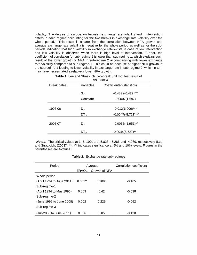
Table-1 reports the result of Lee and Strazicich break test for exchange rate
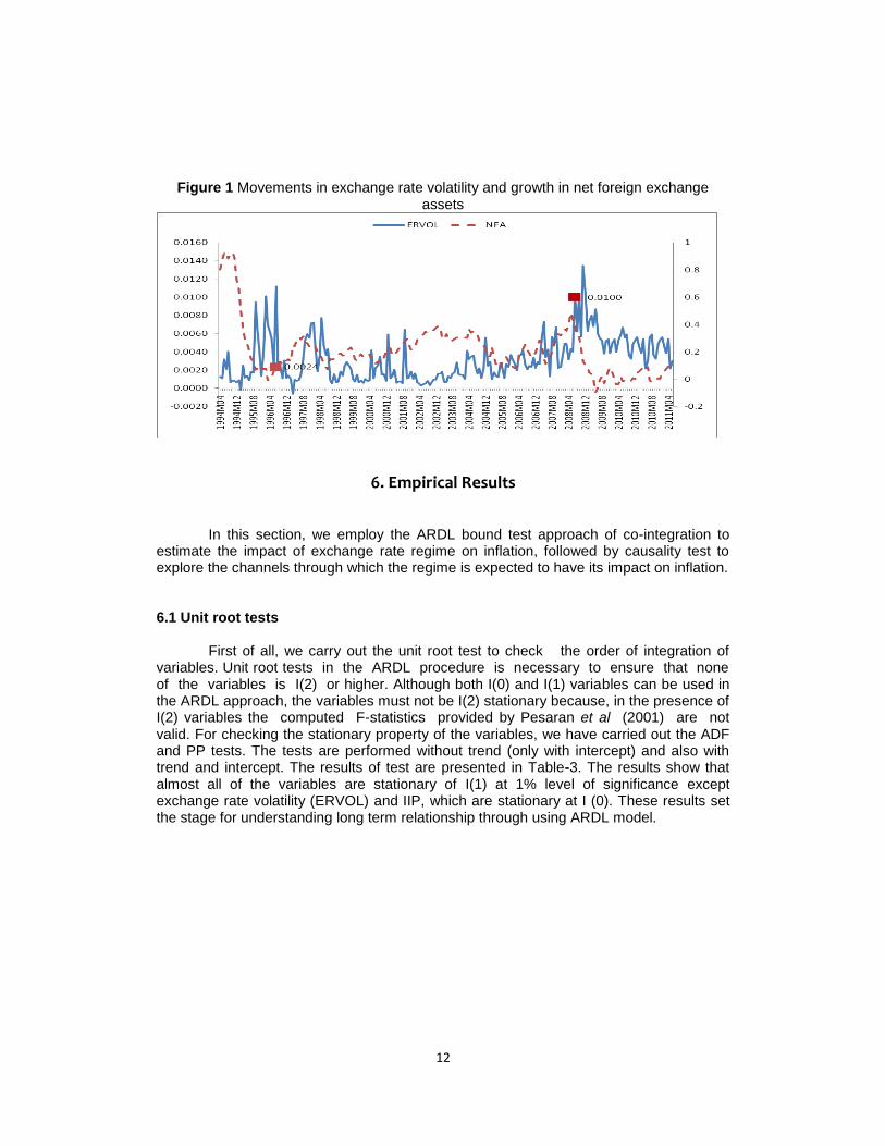
volatility for the sample period 1994 April to 2011 June. The significance of the test statistic confirms that exchange rate volatility series is stationary with breaks at 1996 June and 2008 July, thus pointing to the existence of three de facto sub-regimes within the official managed float regime. While average exchange rate volatility has been low 0.0032 for the whole period indicating a de facto stable exchange rate regime in place for the whole period, it has been lower (0.002) in sub-regime -2 than in sub-regime -1(0.003) and sub regime-3 (0.006) as shown in Figure-1. Figure 1 and Table 2 depict the growth of Net foreign exchange (NFA) assets along with exchange rate volatility which shows higher NFA growth during the periods of low exchange rate volatility and lower NFA growth for the period of high volatility in exchange rate except the sub-regime 2, which has a lower NFA growth than the sub-regime-1, a period of higher exchange rate
3 Although IIP is known to be crude proxy for output, this is a well-known limitation for any empirical
studies based on monthly data. In the absence of monthly data on GDP, exports plus imports is used as a measure of openness instead of the same as a ratio to GDP.
11
volatility. The degree of association between exchange rate volatility and intervention differs in each regime accounting for the two breaks in exchange rate volatility over the whole period. This result is clearer from the correlation between NFA growth and average exchange rate volatility is negative for the whole period as well as for the sub-periods indicating that high volatility in exchange rate exists in case of low intervention and low volatility is observed when there is high level of intervention. Further, the coefficient of correlation for sub regime-2 is lower than sub regime 1, which explains such result of the lower growth of NFA in sub-regime 2 accompanying with lower exchange rate volatility compared to sub-regime-1. This could be because of higher NFA growth in the subregime-1 leading to lower volatility in exchange rate in sub-regime 2, which in turn may have necessitated a relatively lower NFA growth.
Notes: The critical values at 1, 5, 10% are -5.823, -5.286 and -4.989, respectively (Lee
and Strazicich, (2003)). **, *** indicates significance at 5% and 10% levels. Figures in the parentheses are t-values.
Table 2: Exchange rate sub-regimes
Period Average Correlation coefficient
ERVOL Growth of NFA
Whole period
0.0032 0.2098 -0.165 (April 1994 to June 2011)
Sub-regime-1
0.003 0.42 -0.538 (April 1994 to May 1996)
Sub-regime-2
0.002 0.225 -0.062 (June 1996 to June 2008)
Sub-regime-3
0.006 0.05 -0.138 (July2008 to June 2011)
Table 1: Lee and Strazicich two-break unit root test result of ERVOL(k=5)
Break dates Variables Coefficients(t-statistics)
St-1 -0.489 (-6.427)***
Constant 0.0007(1.697)
1996:06 D1t 0.012(6.009)***
DT1t -0.0047(-5.723)***
2008:07 D2t -0.0036(-1.951)**
DT2t 0.0044(5.727)***
12
Figure 1 Movements in exchange rate volatility and growth in net foreign exchange assets
6. Empirical Results
In this section, we employ the ARDL bound test approach of co-integration to estimate the impact of exchange rate regime on inflation, followed by causality test to explore the channels through which the regime is expected to have its impact on inflation. 6.1 Unit root tests
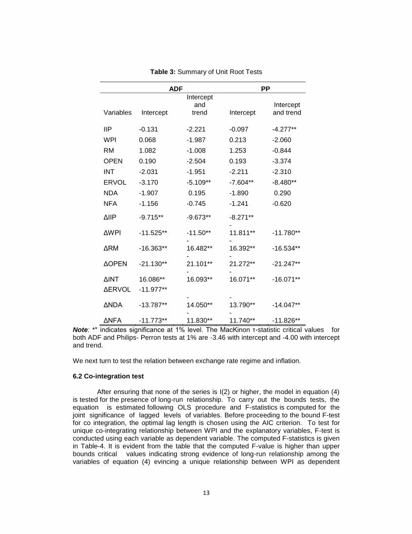
First of all, we carry out the unit root test to check the order of integration of variables. Unit root tests in the ARDL procedure is necessary to ensure that none of the variables is I(2) or higher. Although both I(0) and I(1) variables can be used in the ARDL approach, the variables must not be I(2) stationary because, in the presence of I(2) variables the computed F-statistics provided by Pesaran et al (2001) are not valid. For checking the stationary property of the variables, we have carried out the ADF and PP tests. The tests are performed without trend (only with intercept) and also with trend and intercept. The results of test are presented in Table-3. The results show that almost all of the variables are stationary of I(1) at 1% level of significance except exchange rate volatility (ERVOL) and IIP, which are stationary at I (0). These results set the stage for understanding long term relationship through using ARDL model.
13
Table 3: Summary of Unit Root Tests
ADF PP
Variables Intercept
Intercept and
trend Intercept Intercept and trend
IIP -0.131
-2.221
-0.097
-4.277**
WPI 0.068
-1.987
0.213
-2.060
RM 1.082
-1.008
1.253
-0.844
OPEN 0.190
-2.504
0.193
-3.374
INT -2.031
-1.951
-2.211
-2.310
ERVOL -3.170
-5.109**
-7.604**
-8.480**
NDA -1.907
0.195
-1.890
0.290
NFA -1.156
-0.745
-1.241
-0.620
ΔIIP -9.715**
-9.673**
-8.271**
ΔWPI -11.525**
-11.50**
-11.811**
-11.780**
ΔRM -16.363**
-16.482**
-16.392**
-16.534**
ΔOPEN -21.130**
-21.101**
-21.272**
-21.247**
ΔINT 16.086**
-16.093**
-16.071**
-16.071**
ΔERVOL -11.977**
ΔNDA -13.787**
-14.050**
-13.790**
-14.047**
ΔNFA -11.773** -11.830**
-11.740** -11.826**
Note: ** indicates significance at 1% level. The MacKinon τ-statistic critical values for both ADF and Philips- Perron tests at 1% are -3.46 with intercept and -4.00 with intercept and trend. We next turn to test the relation between exchange rate regime and inflation. 6.2 Co-integration test
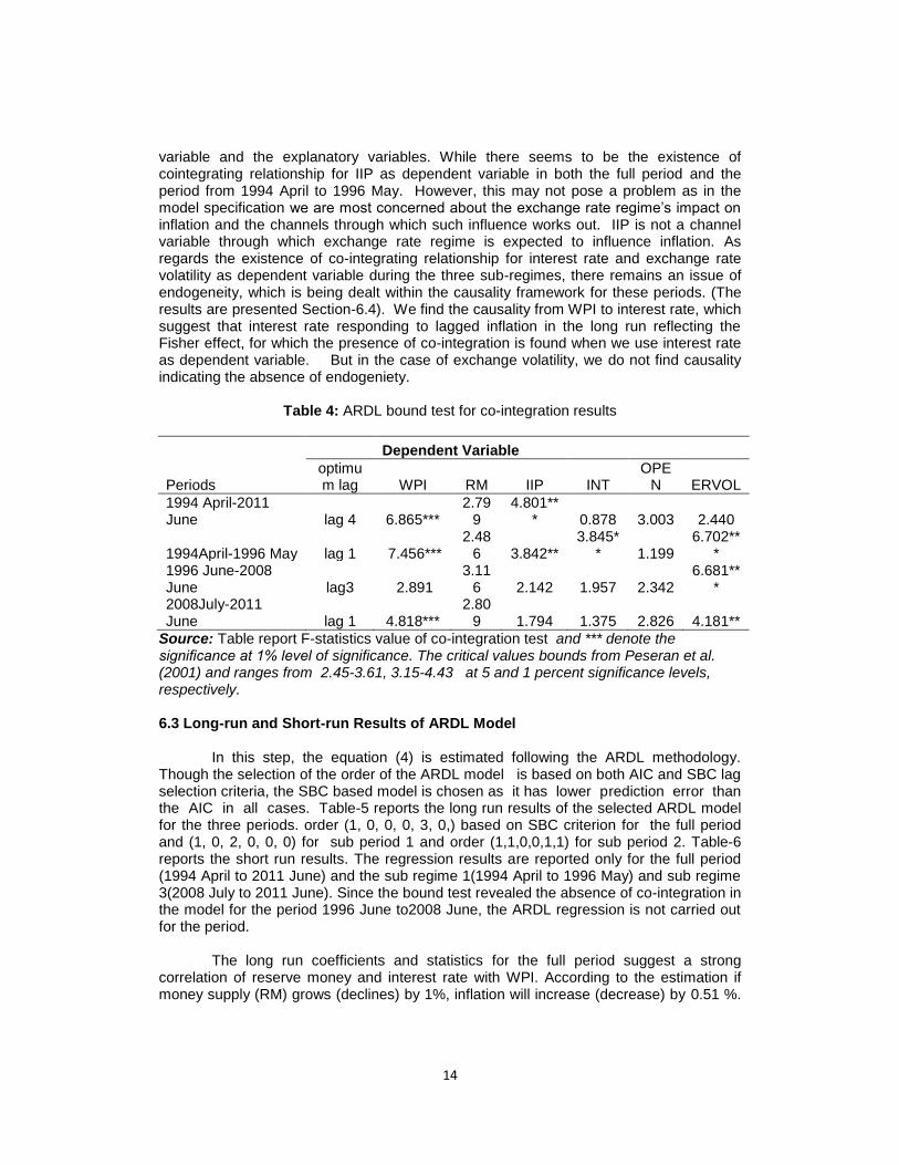
After ensuring that none of the series is I(2) or higher, the model in equation (4) is tested for the presence of long-run relationship. To carry out the bounds tests, the equation is estimated following OLS procedure and F-statistics is computed for the joint significance of lagged levels of variables. Before proceeding to the bound F-test for co integration, the optimal lag length is chosen using the AIC criterion. To test for unique co-integrating relationship between WPI and the explanatory variables, F-test is conducted using each variable as dependent variable. The computed F-statistics is given in Table-4. It is evident from the table that the computed F-value is higher than upper bounds critical values indicating strong evidence of long-run relationship among the variables of equation (4) evincing a unique relationship between WPI as dependent
14
variable and the explanatory variables. While there seems to be the existence of cointegrating relationship for IIP as dependent variable in both the full period and the period from 1994 April to 1996 May. However, this may not pose a problem as in the model specification we are most concerned about the exchange rate regime’s impact on inflation and the channels through which such influence works out. IIP is not a channel variable through which exchange rate regime is expected to influence inflation. As regards the existence of co-integrating relationship for interest rate and exchange rate volatility as dependent variable during the three sub-regimes, there remains an issue of endogeneity, which is being dealt within the causality framework for these periods. (The results are presented Section-6.4). We find the causality from WPI to interest rate, which suggest that interest rate responding to lagged inflation in the long run reflecting the Fisher effect, for which the presence of co-integration is found when we use interest rate as dependent variable. But in the case of exchange volatility, we do not find causality indicating the absence of endogeniety.
Table 4: ARDL bound test for co-integration results
Dependent Variable
Periods optimum lag WPI RM IIP INT
OPEN ERVOL
1994 April-2011 June lag 4 6.865***
2.799
4.801*** 0.878 3.003 2.440
1994April-1996 May lag 1 7.456*** 2.48
6 3.842** 3.845*
* 1.199 6.702**
* 1996 June-2008 June lag3 2.891
3.116 2.142 1.957 2.342
6.681***
2008July-2011 June lag 1
4.818***
2.809 1.794 1.375 2.826 4.181**
Source: Table report F-statistics value of co-integration test and *** denote the significance at 1% level of significance. The critical values bounds from Peseran et al. (2001) and ranges from 2.45-3.61, 3.15-4.43 at 5 and 1 percent significance levels, respectively. 6.3 Long-run and Short-run Results of ARDL Model
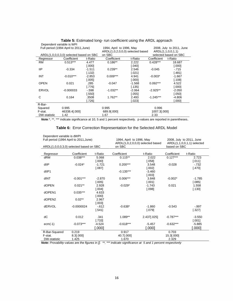
In this step, the equation (4) is estimated following the ARDL methodology. Though the selection of the order of the ARDL model is based on both AIC and SBC lag selection criteria, the SBC based model is chosen as it has lower prediction error than the AIC in all cases. Table-5 reports the long run results of the selected ARDL model for the three periods. order (1, 0, 0, 0, 3, 0,) based on SBC criterion for the full period and (1, 0, 2, 0, 0, 0) for sub period 1 and order (1,1,0,0,1,1) for sub period 2. Table-6 reports the short run results. The regression results are reported only for the full period (1994 April to 2011 June) and the sub regime 1(1994 April to 1996 May) and sub regime 3(2008 July to 2011 June). Since the bound test revealed the absence of co-integration in the model for the period 1996 June to2008 June, the ARDL regression is not carried out for the period.
The long run coefficients and statistics for the full period suggest a strong correlation of reserve money and interest rate with WPI. According to the estimation if money supply (RM) grows (declines) by 1%, inflation will increase (decrease) by 0.51 %.
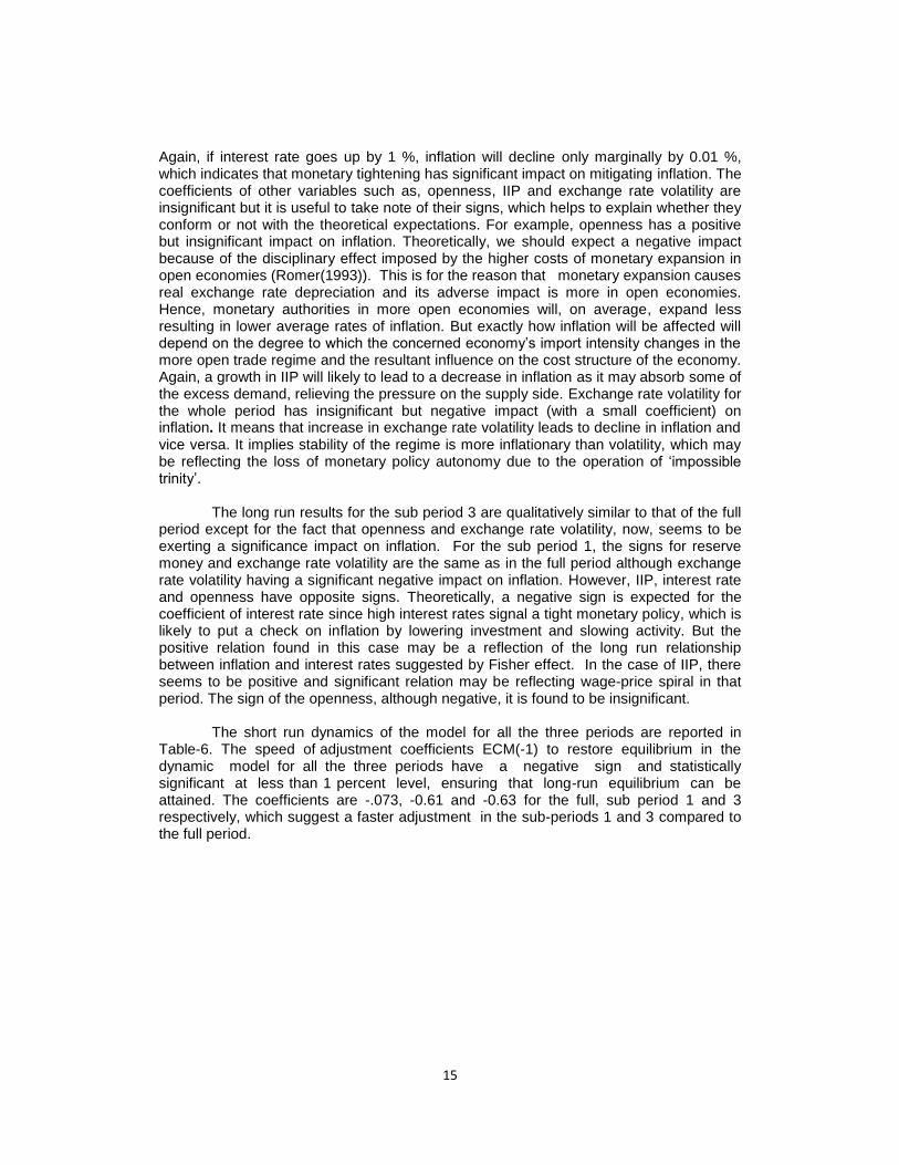
15
Again, if interest rate goes up by 1 %, inflation will decline only marginally by 0.01 %, which indicates that monetary tightening has significant impact on mitigating inflation. The coefficients of other variables such as, openness, IIP and exchange rate volatility are insignificant but it is useful to take note of their signs, which helps to explain whether they conform or not with the theoretical expectations. For example, openness has a positive but insignificant impact on inflation. Theoretically, we should expect a negative impact because of the disciplinary effect imposed by the higher costs of monetary expansion in open economies (Romer(1993)). This is for the reason that monetary expansion causes real exchange rate depreciation and its adverse impact is more in open economies. Hence, monetary authorities in more open economies will, on average, expand less resulting in lower average rates of inflation. But exactly how inflation will be affected will depend on the degree to which the concerned economy’s import intensity changes in the more open trade regime and the resultant influence on the cost structure of the economy. Again, a growth in IIP will likely to lead to a decrease in inflation as it may absorb some of the excess demand, relieving the pressure on the supply side. Exchange rate volatility for the whole period has insignificant but negative impact (with a small coefficient) on inflation. It means that increase in exchange rate volatility leads to decline in inflation and vice versa. It implies stability of the regime is more inflationary than volatility, which may be reflecting the loss of monetary policy autonomy due to the operation of ‘impossible trinity’.
The long run results for the sub period 3 are qualitatively similar to that of the full period except for the fact that openness and exchange rate volatility, now, seems to be exerting a significance impact on inflation. For the sub period 1, the signs for reserve money and exchange rate volatility are the same as in the full period although exchange rate volatility having a significant negative impact on inflation. However, IIP, interest rate and openness have opposite signs. Theoretically, a negative sign is expected for the coefficient of interest rate since high interest rates signal a tight monetary policy, which is likely to put a check on inflation by lowering investment and slowing activity. But the positive relation found in this case may be a reflection of the long run relationship between inflation and interest rates suggested by Fisher effect. In the case of IIP, there seems to be positive and significant relation may be reflecting wage-price spiral in that period. The sign of the openness, although negative, it is found to be insignificant.
The short run dynamics of the model for all the three periods are reported in
Table-6. The speed of adjustment coefficients ECM(-1) to restore equilibrium in the dynamic model for all the three periods have a negative sign and statistically significant at less than 1 percent level, ensuring that long-run equilibrium can be attained. The coefficients are -.073, -0.61 and -0.63 for the full, sub period 1 and 3 respectively, which suggest a faster adjustment in the sub-periods 1 and 3 compared to the full period.
16
Table 5: Estimated long- run coefficient using the ARDL approach Dependent variable is WPI Full period (1994 April to 2011,June) 1994, April to 1996, May 2008, July to 2011, June
ARDL(1,0,0,0,3,0) selected based on SBC ARDL(1,0,2,0,0,0) selected based on SBC
ARDL(1,1,0,0,1,1) selected based on SBC
Regressor Coefficient t-Ratio Coefficient t-Ratio Coefficient t-Ratio
RM 0.513*** 4.477 0.186** 2.222 0.428*** 18.687
[.000]
[.040]
[.000]
IIP -0.334 -1.511 0.239** 2.546 -0.045 -.715
[.132]
[.021]
[.481]
INT -0.010*** -2.853 0.009*** 4.941 -0.003* -1.667
[.005]
[.000]
[.108]
OPEN 0.021 .285 -0.047 -1.568 0.092*** 4.522
[.776]
[.135]
[.000]
ERVOL -0.000033 -.598 -1.032** -2.064 -2.925** -2.050
[.550]
[.055]
[.050]
C 0.164 .3508 1.762** 2.493 -1.245*** -4.806
[.726]
[.023]
[.000]
R-Bar-Squared 0.995 0.995 0.996 F-stat. 46338.4[.000]
689.9[.000]
1007.3[.000]
DW-statistic 1.42 1.67 2.33
Note:*, **, *** indicate significance at 10, 5 and 1 percent respectively. p-values are reported in parentheses.
Table 6: Error Correction Representation for the Selected ARDL Model
Dependent variable is dWPI Full period (1994 April to 2011,June) 1994, April to 1996, May 2008, July to 2011, June
ARDL(1,0,0,0,3,0) selected based on SBC ARDL(1,0,2,0,0,0) selected based on SBC
ARDL(1,1,0,0,1,1) selected based on SBC
Regressor
Coefficient t-Ratio Coefficient t-Ratio Coefficient t-Ratio
dRM 0.038*** 5.068 0.115** 2.022 0.127*** 2.723
[.000]
[.058]
[.011]
dIIP -0.024* -1.721 0.200*** 3.548 -0.028 -.732
[.087]
[.002]
[.470]
dIIP1
-0.135*** -3.460
[.003]
dINT -0.001*** -2.870 0.006*** 3.848 -0.002* -1.785
[.005]
[.001]
[.085]
dOPEN 0.021** 2.928 -0.029* -1.743 0.021 1.558
[.004]
[.098]
[.130]
dOPEN1 0.035*** 4.633
[.000]
dOPEN2 0.02** 2.967
[.003]
dERVOL -0.0000024 -.612 -0.638* -1.860 -0.543 -.997
[.541]
[.079]
[.327]
dC 0.012 .341 1.089**
2.437[.025] -0.787*** -3.550
[.733]
[.001]
ecm(-1) -0.073*** -4.524 -0.618*** -5.457 -0.632*** -5.885
[.000]
[.000]
[.000]
R-Bar-Squared 0.219 0.917
0.703 F-stat. 8.3[.000]
40.7[.000]
15.3[.000]
DW-statistic 1.425 1.670
2.329 Note: Provability-values are the figures in []. **, *** indicate significance at 5 and 1 percent respectively
17
Table 7: Diagnostic tests
Full Period 1994,April-1996,May 2008,July-2011,June
ARCH TEST 1.291[.275] .427[.660] .241[.627] LM Serial Correlation 1.414[.162] .584[.456] 2.018[.155] Ramsey's RESET test 3.691[.056] 1.068[.317] .271[.607]
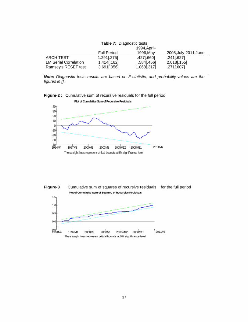
Note: Diagnostic tests results are based on F-statistic, and probability-values are the figures in []. Figure-2 : Cumulative sum of recursive residuals for the full period
Plot of Cumulative Sum of Recursive Residuals
The straight lines represent critical bounds at 5% significance level
-10
-20
-30
-40
0
10
20
30
40
1994M4 1997M3 2000M2 2003M1 2005M12 2008M11 2011M6
Figure-3 Cumulative sum of squares of recursive residuals for the full period
Plot of Cumulative Sum of Squares of Recursive Residuals
The straight lines represent critical bounds at 5% significance level
-0.5
0.0
0.5
1.0
1.5
1994M4 1997M3 2000M2 2003M1 2005M12 2008M11 2011M6
18
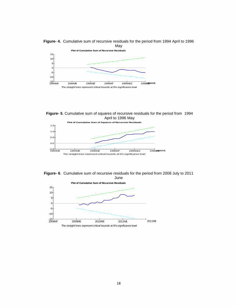
Figure- 4. Cumulative sum of recursive residuals for the period from 1994 April to 1996 May
Plot of Cumulative Sum of Recursive Residuals
The straight lines represent critical bounds at 5% significance level
-5
-10
-15
0
5
10
15
1994M4 1994M9 1995M2 1995M7 1995M12 1996M51996M5
Figure- 5. Cumulative sum of squares of recursive residuals for the period from 1994 April to 1996 May
Plot of Cumulative Sum of Squares of Recursive Residuals
The straight lines represent critical bounds at 5% significance level
-0.5
0.0
0.5
1.0
1.5
1994M4 1994M9 1995M2 1995M7 1995M12 1996M51996M5
Figure- 6. Cumulative sum of recursive residuals for the period from 2008 July to 2011
June
Plot of Cumulative Sum of Recursive Residuals
The straight lines represent critical bounds at 5% significance level
-5
-10
-15
0
5
10
15
2008M7 2009M5 2010M3 2011M1 2011M6
19
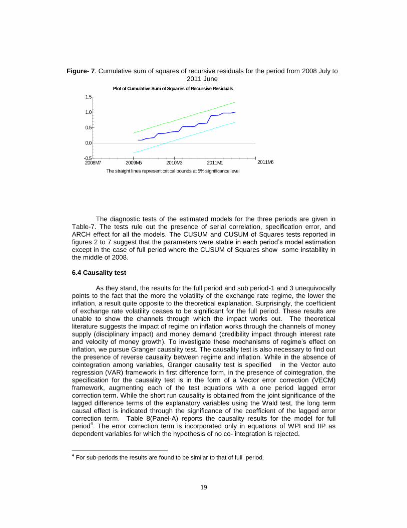
Figure- 7. Cumulative sum of squares of recursive residuals for the period from 2008 July to 2011 June
Plot of Cumulative Sum of Squares of Recursive Residuals
The straight lines represent critical bounds at 5% significance level
-0.5
0.0
0.5
1.0
1.5
2008M7 2009M5 2010M3 2011M1 2011M6
The diagnostic tests of the estimated models for the three periods are given in
Table-7. The tests rule out the presence of serial correlation, specification error, and ARCH effect for all the models. The CUSUM and CUSUM of Squares tests reported in figures 2 to 7 suggest that the parameters were stable in each period’s model estimation except in the case of full period where the CUSUM of Squares show some instability in the middle of 2008. 6.4 Causality test As they stand, the results for the full period and sub period-1 and 3 unequivocally points to the fact that the more the volatility of the exchange rate regime, the lower the inflation, a result quite opposite to the theoretical explanation. Surprisingly, the coefficient of exchange rate volatility ceases to be significant for the full period. These results are unable to show the channels through which the impact works out. The theoretical literature suggests the impact of regime on inflation works through the channels of money supply (disciplinary impact) and money demand (credibility impact through interest rate and velocity of money growth). To investigate these mechanisms of regime’s effect on inflation, we pursue Granger causality test. The causality test is also necessary to find out the presence of reverse causality between regime and inflation. While in the absence of cointegration among variables, Granger causality test is specified in the Vector auto regression (VAR) framework in first difference form, in the presence of cointegration, the specification for the causality test is in the form of a Vector error correction (VECM) framework, augmenting each of the test equations with a one period lagged error correction term. While the short run causality is obtained from the joint significance of the lagged difference terms of the explanatory variables using the Wald test, the long term causal effect is indicated through the significance of the coefficient of the lagged error correction term. Table 8(Panel-A) reports the causality results for the model for full period
4. The error correction term is incorporated only in equations of WPI and IIP as
dependent variables for which the hypothesis of no co- integration is rejected.
4 For sub-periods the results are found to be similar to that of full period.
20
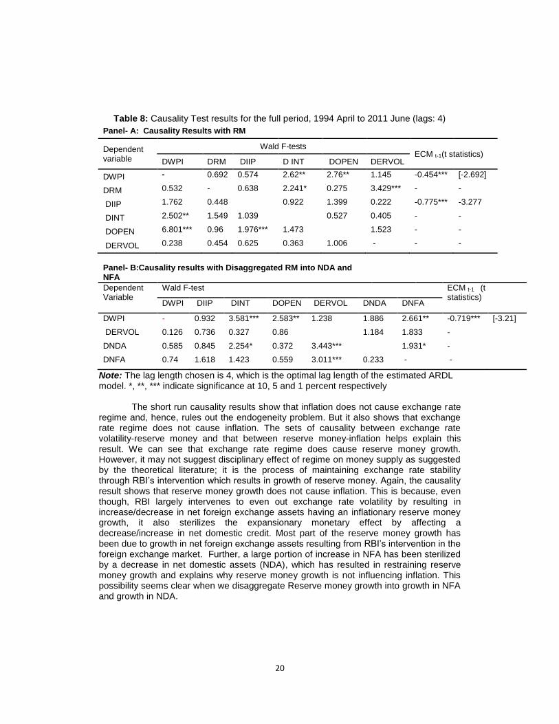
Table 8: Causality Test results for the full period, 1994 April to 2011 June (lags: 4)
Panel- A: Causality Results with RM
Dependent variable
Wald F-tests ECM t-1(t statistics)
DWPI DRM DIIP D INT DOPEN DERVOL
DWPI - 0.692 0.574 2.62** 2.76** 1.145 -0.454*** [-2.692]
DRM 0.532 - 0.638 2.241* 0.275 3.429*** - -
DIIP 1.762 0.448 0.922 1.399 0.222 -0.775*** -3.277
DINT 2.502** 1.549 1.039 0.527 0.405 - -
DOPEN 6.801*** 0.96 1.976*** 1.473 1.523 - -
DERVOL 0.238 0.454 0.625 0.363 1.006 - - -
Panel- B:Causality results with Disaggregated RM into NDA and NFA
Dependent Variable
Wald F-test ECM t-1 (t statistics)
DWPI DIIP DINT DOPEN DERVOL DNDA DNFA
DWPI - 0.932 3.581*** 2.583** 1.238 1.886 2.661** -0.719*** [-3.21]
DERVOL 0.126 0.736 0.327 0.86 1.184 1.833 -
DNDA 0.585 0.845 2.254* 0.372 3.443*** 1.931* -
DNFA 0.74 1.618 1.423 0.559 3.011*** 0.233 - -
Note: The lag length chosen is 4, which is the optimal lag length of the estimated ARDL model. *, **, *** indicate significance at 10, 5 and 1 percent respectively
The short run causality results show that inflation does not cause exchange rate regime and, hence, rules out the endogeneity problem. But it also shows that exchange rate regime does not cause inflation. The sets of causality between exchange rate volatility-reserve money and that between reserve money-inflation helps explain this result. We can see that exchange rate regime does cause reserve money growth. However, it may not suggest disciplinary effect of regime on money supply as suggested by the theoretical literature; it is the process of maintaining exchange rate stability through RBI’s intervention which results in growth of reserve money. Again, the causality result shows that reserve money growth does not cause inflation. This is because, even though, RBI largely intervenes to even out exchange rate volatility by resulting in increase/decrease in net foreign exchange assets having an inflationary reserve money growth, it also sterilizes the expansionary monetary effect by affecting a decrease/increase in net domestic credit. Most part of the reserve money growth has been due to growth in net foreign exchange assets resulting from RBI’s intervention in the foreign exchange market. Further, a large portion of increase in NFA has been sterilized by a decrease in net domestic assets (NDA), which has resulted in restraining reserve money growth and explains why reserve money growth is not influencing inflation. This possibility seems clear when we disaggregate Reserve money growth into growth in NFA and growth in NDA.
21
The causality test result with disaggregated reserve money is also reported (Panel-B).The causality running from NFA to NDA is indicative of the sterilization undertaken by RBI by a contraction in NDA in the face of an increase in NFA. Further, it is evident from the causality results that exchange rate volatility causes NFA growth and NFA growth causes Inflation but simultaneously exchange rate volatility causes NDA growth offsetting the growth in NFA, which explains the earlier causality test results of the ineffectiveness of reserve money growth in causing inflation.
The long run causality from reserve money, IIP, openness, interest rate with WPI is supported by the negative and significant coefficient of the error correction term in the equation for WPI, which means that the WPI series is non-explosive and equilibrium in the long run is attainable.
7. Conclusion and Policy Implication
While India has made a transition from relatively fixed exchange rate regime to a managed float regime, as claimed officially, the existing studies show that the de facto regime behavior has exhibited considerable stability. This is because of large intervention by the central bank to manage exchange rate volatility. The literature on the assessment of the optimal exchange rate regime favors stable exchange rate regime for inflation consequences; a stable exchange rate is considered less inflationary than a more flexible regime as it has a restrictive impact on the determinants of inflation such as, money supply and money demand. Seeking to find whether exchange rate stability in the so called managed float regime has led to lower inflation, we find that it is not the exchange rate stability or volatility per se that has led to low inflation, but, rather, the sterilized intervention of RBI, which has kept a check on reserve money growth and its inflationary consequences resulting from its attempt to maintain a stable exchange rate. Hence, the seemingly conflicting result of the association of inflation and exchange rate volatility in the regression result for the full period and sub periods disappears in the causality test as low inflation is not the result of disciplinary effect of the pegged or stable exchange rate regime in India, rather it is the less reserve money growth as an outcome of central bank’s sterilized intervention. The result points to the loss of monetary policy autonomy due to the ‘impossible trinity’ coming to play with steady increase of capital inflows. So, the Indian case is not one conforming to the popular view that pegged or stable exchange rate is helpful for inflation, as it merely reflects the success of central bank in neutralizing its very effort of maintaining the pegged rate which gives rise to inflationary growth of money supply. In the absence of sterilization, whether the theoretical stable exchange rate-high inflation relationship could hold is an empirical issue.
22
References
Bailliu J., Lafrance R. and Perrault J.F., (2003), “Does Exchange Rate Policy Matter for growth?”, International Finance, 6(3), November,381-414.
Banerjee A, Dolado J, Galbraith J.W., and Hendry D. (1993), Co-integration, Error Correction, and the Econometric Analysis of Non-stationary Data, Oxford: Oxford University Press. Barro, R.J. and Gordon, D.B. (1983b), “Rules, Discretion, and Reputation in a Model of
Monetary Policy”, Journal of Monetary Economics, 12, July,101-121. Benigno, P. and Missale, A., (2004), “High Public Debt in Currency Crises: Fundamental
versus Signaling Effects”, Journal of International Money and Finance, 23(2), March, 165-188.
Bernanke, B.S., Mishkin F.S., Laubach T., and Posen A.S.,(1999), Inflation Targeting:
Lessons From the International Experience, Princeton, Princeton University Press. Bleaney, M. and Francisco, M., (2007), “Exchange Rate Regime, Inflation and Growth in
Developing Economies – An Assessment”, The BE Journal of Macroeconomics, 7(1), 1- 18.
Calvo, G.A., and C.M. Reinhart, (2000), “Fixing for Your Life,” NBER Working Paper
8006, November. Calvo, G.A, and C.M Reinhart (2002), “Fear of Floating,” Quarterly Journal of Economics,
117 (2), 379-408 Coudert, Virginie and Dubert, Marc, (2005) "Does exchange rate regime explain
differences in economic results for Asian countries?," Journal of Asian Economics, 16(5), 874-895.
De Grauwe, P. and Schnabl, G.,(2004), “Exchange Rates Regimes and Macroeconomic
Stability in Central and Eastern Europe”, CESifo Working Paper, 1182,April,1-34. Domac, I., Peters, K., and Yuzefovich, Y.,(2001), “Does the Exchange Rate Regime
Affect Macroeconomic Performance? Evidence from Transition Economies”, Policy Research Working Paper Series 2642,World Bank.
Dornbusch, R. (2001), "Fewer Monies, Better Monies," NBER Working Paper 8324. Enders,W.(2004), Applied Econometric Time series, Published by John Wiley and Sons, second edition. Garofalo, P.,(2005), “Exchange Rate Regimes and Economic Performance: The Italian
Experience”, Banca D’Italia Quaderni dell’Úfficio Ricerche Storiche, 10,September, 1-50.
23
Ghosh, A.R., Ostry, J.D., Gulde, A.M. and Wolf, H.C., (1997), “Does the Nominal Exchange Rate Regime Matter?” NBER Working Paper.5874
Ghosh, Atish R., Gulde, Anne-Marie, and Wolf, Holger C., (2003), Consequences, The
MIT Press, edition 1, volume 1. Giavazzi, Francesco and Giovannini, Alberto, (1989), Limiting Exchange Rate Flexibility,
Cambridge, the MIT Press. Hernandez-Verme, Paula,(2004), “Inflation, Growth and Exchange Rate Regimes in
Small Open Economies”, Economic Theory, 24(4), 839- 856. Hutchison, Michael, Sengupta, Rajeswari, and Singh, Nirvikar,(2012), ‘India’s Trilemma:
Financial Liberalisation, Exchange Rates and Monetary Policy’, The World Economy, 35(1),January,3-18
lzetzki E., Reinhart M. Carmen and C. and Rogoff S. Kenneth (2008), “The Country
Chronologies and Background Material to Exchange Rate Arrangements in the 21st Century: Which Anchor Will Hold?”, mimeo, http://terpconnect.umd.edu/~creinhar/Papers/ERA-Country%20chronologies.pdf
IMF,(2010), “India: 2009 Article IV Consultation – Staff Report; Staff Statement; Public
Information Notice On The Executive Board Discussion; And Statement By The Executive Director For India”, IMF Country Report 10/73, March (Washington, DC: IMF).
Lee, Junsoo and Strazicich, Mark C., (2003), "Minimum LM Unit Root Test with Two
Structural Breaks," Review of Economics and Statistics, 85(4),November,1082-1089. Levy-Yeyati, Eduardo and Sturzenegger, Federico.,(2003), “A De Facto Classification of
Exchange Rate Regimes: A Methodological Note”, American Economic Review, 93(4),September.
Levy-Yeyati, Eduardo and Sturzenegger, Federico.,(2005), “Classifying Exchange Rate
Regimes: Deeds vs. Words”, European Economic Review, 49(6), August, 1603-35. Levy-Yeyati, Eduardo and Sturzenegger, Federico.,(2000), Exchange Rate Regime and
Economic Performance, UTDT,CIF Working Paper No. 2/01.. Mundell, Robert A., (1961), "Capital Mobility and Stabilization Policy under Fixed and
Flexible Exchange Rates," Canadian Journal of Economics and Political Science, 29, November, 475 - 485.
Miles, William (2008), “Exchange rates, Inflation and Growth in Small, Open economies:
a Difference-in -Difference Approach”, Applied Economics , 40(3), 341-348. Patel, Urjit R. and Srivastava, Pradeep. (1998), “Some Implications of Real Exchange
Rate Targeting in India”, ICRIER Working Paper No 43, Indian Council for Research on International Economic Relations.
24
Patnaik, Ila, (2003), India’s policy stance on reserves and the currency, Technical report, ICRIER Working Paper No 108, Indian Council for Research on International Economic Relations.
Patnaik, Ila, (2004),"India's Experience with a Pegged Exchange Rate," India Policy
Forum, Global Economy and Development Program, The Brookings Institution, vol. 1(1), pages 189-226.
Patnaik, R. K., Kapur, Muneesh, and Dhal S. C.,(2003), “Exchange Rate Policy and
Management: The Indian Experience”, Economic and Political Weekly, 38(22), May 31 - Jun. 6, 2139-2153
Pesaran M. Hashem, and Pesaran, Bahram, (1997), Working with Microfit 4.0:
Interactive Econometric Analysis, Oxford: Oxford University Press. Pesaran M. Hashem, Shin Yongcheol, and Smith, Richard J., (2001), “Bound Testing
Approaches to the Analysis of Level Relationships”, Journal of Applied Econometrics, 16(3), June,289-326.
Reinhart, C. (2000), “The Mirage of Floating Exchange Rates”, American Economic
Review, 90(2), May 65-70. Reinhart M. Carmen and C. and Rogoff S. Kenneth, (2004), “The Modern History of
Exchange Rate Arrangements: A Reinterpretation”, Quarterly Journal of Economics, 119(1), February, 1-48.
Reserve Bank of India (1993): Report of High Level Committee on Balance of Payments (Chairman: C Rangarajan), RBI Bulletin, August. Romer, David, (1993), "Openness and Inflation: Theory and Evidence," The Quarterly
Journal of Economics, MIT Press, 108(4), November,869-903, Summers, Lawrence H., (2000), “International Financial Crises: Causes, Prevention, and
Cures,” American Economic Review, Papers and Proceedings, 90(2),May,1–16. Tornell A. and Velasco A., (1994), “Fiscal Policy and the Choice of exchange Rate
Regime”, Working Paper No. 247,September, Inter-American Development Bank. Velasco A., (1996), “Fixed Exchange Rates: Credibility, Flexibility and Multiplicity”,
European Economic Review, 40[3-5], April, 1023-1035.