This article was downloaded by: [East Carolina University]On: 17 September 2013, At: 11:17Publisher: RoutledgeInforma Ltd Registered in England and Wales Registered Number: 1072954 Registered office:Mortimer House, 37-41 Mortimer Street, London W1T 3JH, UK

Applied Financial EconomicsPublication details, including instructions for authors and subscriptioninformation:http://www.tandfonline.com/loi/rafe20

Exchange rate and stock price interactions inemerging financial markets: evidence on India,Korea, Pakistan and the PhilippinesIssam S.A. Abdalla & Victor MurindePublished online: 06 Oct 2010.

To cite this article: Issam S.A. Abdalla & Victor Murinde (1997) Exchange rate and stock price interactions inemerging financial markets: evidence on India, Korea, Pakistan and the Philippines, Applied Financial Economics,7:1, 25-35, DOI: 10.1080/096031097333826

To link to this article: http://dx.doi.org/10.1080/096031097333826

PLEASE SCROLL DOWN FOR ARTICLE

Taylor & Francis makes every effort to ensure the accuracy of all the information (the “Content”)contained in the publications on our platform. However, Taylor & Francis, our agents, and ourlicensors make no representations or warranties whatsoever as to the accuracy, completeness, orsuitability for any purpose of the Content. Any opinions and views expressed in this publication arethe opinions and views of the authors, and are not the views of or endorsed by Taylor & Francis.The accuracy of the Content should not be relied upon and should be independently verified withprimary sources of information. Taylor and Francis shall not be liable for any losses, actions, claims,proceedings, demands, costs, expenses, damages, and other liabilities whatsoever or howsoevercaused arising directly or indirectly in connection with, in relation to or arising out of the use of theContent.

This article may be used for research, teaching, and private study purposes. Any substantialor systematic reproduction, redistribution, reselling, loan, sub-licensing, systematic supply, ordistribution in any form to anyone is expressly forbidden. Terms & Conditions of access and use canbe found at http://www.tandfonline.com/page/terms-and-conditions

§ Address all correspondence to Victor Murinde, Department of Accounting and Finance, University of Birmingham, Edgbaston,Birmingham B15 2TT, England.1 According to IFC (1993), the term emerging stock markets refers to any market belonging to low- and middle-income LDCs, with theimplication that all have the potential for development. See also Divecha et al. (1992).

Applied Financial Economics, 1997, 7, 25 Ð 35

Exchange rate and stock price interactionsin emerging Þ nancial markets: evidenceon India, Korea, Pakistan andthe Philippines

ISSAM S.A. ABDALLA and VICTOR MURINDE* §

United Saudi Commercial Bank, Riyadh 11476, Saudi Arabia and *Department ofAccounting and Finance, University of Birmingham, UK

Interactions are investigated between exchange rates and stock prices in the emerging® nancial markets of India, Korea, Pakistan and the Philippines. The motivation is toestablish the causal linkages between leading prices in the foreign exchange marketand the stock market; the linkages have implications for the ongoing attempts todevelop stock markets in emerging economies simultaneously with a policy shifttowards independently ¯ oating exchange rates. Some recent econometric techniquesare applied to a bivariate vector autoregressive model using monthly observations onthe IFC stock price index and the real e� ective exchange rate over 1985:01 Ð 1994 :07.The results show unidirectional causality from exchange rates to stock prices in all thesample countries, except the Philippines. This ® nding has policy implications; itsuggests that respective governments should be cautious in their implementation ofexchange rate policies, given that such policies have rami® cations on their stockmarkets.

I . INTRODUCTION

Two interesting issues that have recently occurred, albeitseparately, in the area of ® nance are the establishment ofstock markets in the emerging economies, and the policy shifttowards independently ¯ oating exchange rates. Some globaleconomic institutions, especially the International FinanceCorporation (IFC), have been encouraging less developedcountries (LDCs) to launch stock markets or revitalize exist-ing ones. It is thought that the creation of emerging stockmarkets (ESMs)1 provides a vehicle for mobilizing savings forprivate sector investment (Hartman and Khambata, 1993). Inparticular, it has been argued that funds raised in the ESMsenable ® rms to decrease their over reliance on debt ® nance,

and to increase overall e� ciency, competitiveness andsolvency (Murinde, 1996). Some ESMs are performing ex-ceptionally well: in 1992 eight of the top 10 places on a list of54 developed and developing stock markets were taken bythe ESMs (IFC, 1993). Notwithstanding the high returnsand rapid growth potential of some ESMs, most of themarkets tend to be very small in size, with very low volumeof transactions, and lack high quality accounting data andother market information. Indeed, Scown (1990) points outthat, given some of the ESMs are still developing, they maybe riskier than their counterparts in industrialized countries.

Meanwhile, the rapid expansion in international tradeduring the 1970s, and the adoption of freely ¯ oating ex-change rate regimes by many industrialized countries in

0960 Ð 3107 Ó 1997 Routledge 25

Dow

nloa

ded

by [

Eas

t Car

olin

a U

nive

rsity

] at

11:

17 1

7 Se

ptem

ber

2013

2 Rst is measured as the dollar price of foreign currency; thus a positive value for Rst indicates a dollar depreciation and a negative valueindicates a dollar appreciation.

1973, heralded a new era of increased exchange rate volatil-ity. Jorion (1990) points out that exchange rates were 4 timesas volatile as interest rates and 10 times as volatile asin¯ ation during the 1980s. Inevitably, the exposure of ® rmsto exchange rate risks has increased (Murinde, 1996). Threedi� erent types of risks under an independently ¯ oatingexchange rate regime are identi® ed in the existing literature:transactions exposure, which arises due to gains or lossesarising from settlement of investment transactions stated inforeign currency terms; economic exposure, which arisesfrom variations in ® rms’ discounted cash ¯ ows when ex-change rates ¯ uctuate; and operating exposure, which is thesensitivity of the home currency value of the ® rm to changesin exchange rates (Ma and Kao, 1990; Loudon, 1993).

This paper brings together the two recent, but separate,developments in the area of ® nance, namely the ESMs andthe adoption of independently ¯ oating exchange rates. It ismotivated to investigate the causal interactions between theleading prices in two components of emerging ® nancialmarkets; namely, exchange rates in the foreign exchangemarket and share prices in the stock market. The maincontributions of the paper are threefold. First, as high-lighted above, the linkages between exchange rates andstock prices bear implications for the ongoing attemptsto develop stock markets in emerging market economiessimultaneously with a policy shift towards independently¯ exible exchange rates. Essentially, we explore the compati-bility of the two policy moves. Second, the paper takes as itstesting ground the main ESMs in the Paci® c Basin andIndia which have recently attracted much attention in themedia and in some policy circles. The newly industrializingcountries have an expanding corporate sector with listed® rms and a growing tradable sector that is sensitive toexchange rates policy. However, due to data availability, werestrict the sample to four economies which have readilyavailable monthly series on stock prices and the real e� ec-tive exchange rate (REER). Third, we call upon some recenteconometric techniques to test for unit root (non-stationar-ity), cointegration, error correction and Granger-causality ,in order to investigate the causal linkages between exchangerates and stock prices.

The rest of this paper is structured into four sections.Section II highlights the main economic underpinningsand empirical ® ndings on the relationship between stockprices and exchange rates. Section III speci® es a bivariatevector autoregressive (BVAR) model as an empiricalframework for investigating causal linkages between stockprices and exchange rates. Section IV reports empiricalprocedures and evidence. Section V o� ers a summary andconclusions.

II . THE ECONOMIC THEORY

It is useful to examine the microeconomic as well as themacroeconomic theoretical foundations of the linkages be-tween exchange rates and stock prices. At the micro level, itis argued that exchange rate changes in¯ uence the valueof a portfolio of domestic and multinational ® rms. Forexample, it is predicted that if the real dollar exchange raterises, ® rms’ pro® ts fall, and so does the ® rm’s share price.See, among others, Jorion (1990). Accordingly, the linkbetween exchange rates and stock prices can be speci® ed asfollows:

R it = b 0 i + b 1 iRst + e it (1)

where Rit = the rate of return on the common stock ofcompany i ; and Rst = the rate of change in a trade-weightedexchange rate;2 and t = 1, ¼ , T . However, the behaviour ofthe stock prices of domestic ® rms tends to di� er from that ofmultinational ® rms. Thus, it is important to determine therelationship between exchange rate exposure and the degreeof foreign involvement, as follows:

b 1 i = a0 + a1 F i + m i (2)

where F i = the ratio of foreign to total sales; i = 1, ¼ , N. Inaddition, the foreign exchange exposure of stocks may beexamined in an extended framework as follows:

R it = b 0 i + b 1 iRst + b 2 iRmt + e it (3)

where Rmt = the return on the domestic stock exchangeaccumulation index in month t. Empirical studies, in thespirit of Equations 1 to 3 suggest that there is generallyweak evidence of exposure of ® rms’ share prices to exchangerate risks. It has, however, been found that resource stocks(gold, other metal, solid fuels, gas and oil industries, etc.) andindustrial stocks (building materials, chemicals, bankingand ® nance, etc.) respond di� erently to ¯ uctuations in theexchange rate. When currency appreciates, industrial stockstend to perform better whereas resource stocks performbetter when currency depreciates (e.g. Loudon, 1993).

At the macro level, the main line of enquiry relates to therelationship between aggregate stock prices and the ¯ oatingvalue of the exchange rate. It is predicted that a negativerelationship exists between the strength of the home cur-rency and the aggregate stock prices index, as given by

Dst = a + b DRSt + cDit + e t (4)

where Dst = change in the real exchange rate; DRSt = thereal stock return di� erential (domestic minus foreign); andDit = the change in interest rate di� erential. Where twodi� erent measures of the aggregate stock price index are

26 I. S. A. Abdalla and V . MurindeD

ownl

oade

d by

[E

ast C

arol

ina

Uni

vers

ity]

at 1

1:17

17

Sept

embe

r 20

13

3 See Granger (1969). The speci® cation of this well-established empirical method, in the context of EX and SP, is obtainable on requestfrom the authors.4 Thus, instantaneous causality is established when the inclusion of the present values of the independent variable improves the predictionor goodness of ® t (or R2 ) of both equations.

quoted, for example the New York Stock Exchange Index(NY SEI ) and the S&P500 Index (S&P500I ) for the US stockmarket, the speci® cation is given by

NY SEI = a1 + b 1 XR + m 1 (5)

S&P500I = a2 + b 2 XR + m 2 (6)

l1 = a3 + b 3 XR + m 3 (7)

where l i = the index of industrial sector i; and XR = broadmeasure of the value of the e� ective exchange rate. How-ever, the above speci® cations may be sensitive to the ex-change rate regime in force. For example, economic theorysuggests that, under a ¯ oating exchange rate regime, ex-change rate appreciation reduces the competitiveness ofexport markets; it therefore has a negative e� ect on thedomestic stock market. Conversely, for an import de-nominated country, exchange rate appreciation lowers in-put costs and generates a positive impact on the stockmarket. Thus, in a macroeconomic framework, the relation-ship between exchange rates and stock prices can best becaptured by including other macro variables in the model.Following Smith (1992a) such a broad model is speci® ed asfollows:

Eug = a 0 + a 1 Euj - a 2 Rgu + a 3 Rj u + a 4 Sg + a 5 Sj

+ a 6 Su + a 7 Ag+ a 8 Aj + a 9 Au

+ a 1 0 (Ag - Ag(D)g ) - a 1 1 CCASg (8)

Euj = b 0 + b 1 Eug + b 2 Rgu - b 3 Rj u + b 4 Sg+ b 5 Sj

+ b 6 Su + b 7 Ag + b 8 Aj + b 9 Au

+ b 1 0 (Aj - Aj (D)j ) - b 1 1 CCASj (9)

where Eug = US Ð German exchange rate; Ag(D)g = the debt

of the German government; Euj = US Ð Japanese ex-change rate; CCASg = the German current account surplus;CCASj = the Japanese current account surplus; Rgu =the German Ð US interest rate di� erentials; Rj u = theJapanese Ð US interest rate di� erential; Sj , Su , Sg = theJapanese, US and German equity values, respectively;Aj , Au , Ag = the Japanese, US and German bond values,respectively; and (Aj - Aj (D)

j ) = the debt of the Japanesegovernment. Empirical studies, based on the speci® cationswhich follow Equations 4 to 9, have uncovered mixed re-sults. On the one hand, it has been found that a signi® cantpositive relationship exists between equity prices and ex-change rates (Smith, 1992a; Solnik, 1987). On the otherhand, it has been shown that, as predicted by economictheory, a strong negative relationship exists between stockprices and exchange rates (Soenen and Hennigar, 1988).

In all, at the macro and micro levels, there is neithera theoretical nor an empirical consensus on the relationshipbetween exchange rates and stock prices. Speci® cally, thecausal direction between the two ® nancial price variables isnot resolved. Furthermore, none of the previous studiesinvestigated this issue with respect to emerging markets forwhich the issue has great policy relevance. It is intended inthis paper to draw on the recent developments in econo-metrics to set up a framework for testing this issue in thelight of experience in the Paci® c Basin. We depart from theprevious literature which has attempted to test each of theabove reviewed theories in isolation; rather, we designa BVAR model as a statistical framework that encapsulatesthe main theories.

III . MODEL

In studying the relationship between exchange rates andstock prices, we need to establish whether changes in stockprices causally a� ect exchange rates or vice versa. Althoughthere are many approaches to modelling causality in tem-poral systems, we ® rst apply the prototype model by Gran-ger (1969) not only because it is the simplest and moststraightforward, but also the existence of causal ordering inGranger’s sense points to a low of causation and impliespredictability and exogeneity. We therefore consider Gran-ger’s four de® nitions of causality, based on the followingBVAR model:

EXt =m

+j = 1

a j EXt ± j +n

+j = 1

b j SPt ± j + e t (10)

SPt =m

+j = 1

cj EXt ± j +n

+j = 1

dj SPt ± j + m t (11)

where EX = exchange rate variable; SP = stock price vari-able; and e t , m t are assumed to be serially uncorrelated withzero mean and ® nite covariance matrix. Granger (1969)o� ers four de® nitions of causality, which in this contextcomprise unidirectional causality from EX to SP; uni-directional causality from SP to EX; feedback causalitybetween EX and SP; and independence between EX andSP.3

The four de® nitions, according to Granger, imply that forSP to Granger-cause EX, the coe� cient b j ¹ 0 in Equation10, whereas cj = 0 in Equation 11; and for EX to Granger-cause SP, cj ¹ 0 whereas b j = 0. If we allow for the possibili-ty of j = 0 in the summation symbol for Equations 10 and11, the relationship between the two time series is said to beinstantaneous.4

Exchange rate and stock price in emerging markets 27D

ownl

oade

d by

[E

ast C

arol

ina

Uni

vers

ity]

at 1

1:17

17

Sept

embe

r 20

13

5 The REER is an index which adjusts the nominal e� ective exchange rate index (itself a trade-weighted average value of a currency againstthe currencies of the corresponding country’s principal trade partners) for relative price changes; it gauges the e� ect of currency changesand di� erential in¯ ation on the international price competitiveness of the countries’ tradables. The weights for the broad index arecalculated in relation to currencies for 18 industrialized countries and 22 LDCs. On the theory of indices of e� ective exchange rates, seeRhomberg (1981).6 Our DF and ADF test are based on the following:

D SPt = a 0 + b 1 T + l 1 SPt ± 1 +n

+i= 1

a i D SPt ± 1 + e 1 t (A)

D EXt = a 0 + b 2 T + l 2 EXt ± 1 +r

+i= 1

/ i D EXt ± 1 + e 2 t (B)

where, D = ® rst di� erence operator, hence D SPt = SPt - SPt ± 1 and D EXt = EXt - EXt ± 1 ; a 0 , b 1 , b 2 , l 1 , l 2 , a i , / i are the coe� cients;T = time trend; and e 1 t and e 2 t are white noise errors. In the DF test S a i = S / i = 0; in the ADF test n and r are chosen so that e 1 t and e 2 t,respectively, are white noise. The null hypothesis (H0 ) is that SPt and EXt have unit roots, that is H0 : l 1 = l 2 = 1. The alternativehypothesis (H1 ) is that both variables are I (0). The null hypothesis is rejected if l 1 and l 2 are signi® cantly negative and t-statistics are less(or greater in absolute values) than the critical values in Fuller (1976).7 We run the following cointegrating regressions for each country:

SPt = aEXt + c + n (A)

The null hypothesis is H0 : EXt , SPt not cointegrated. Using the residuals n t , we run the following regression:

D n t = / n t ± 1 + b 1 D n t ± 1 + ¼ + b p D n t ± p + m t (B)

If the computed ADF (= t / , the t-statistic for / ) is greater than the critical, we reject the null (Engle and Granger, 1987).8 Detailed results for cointegration are not reported here; these can be obtained from the authors on request.

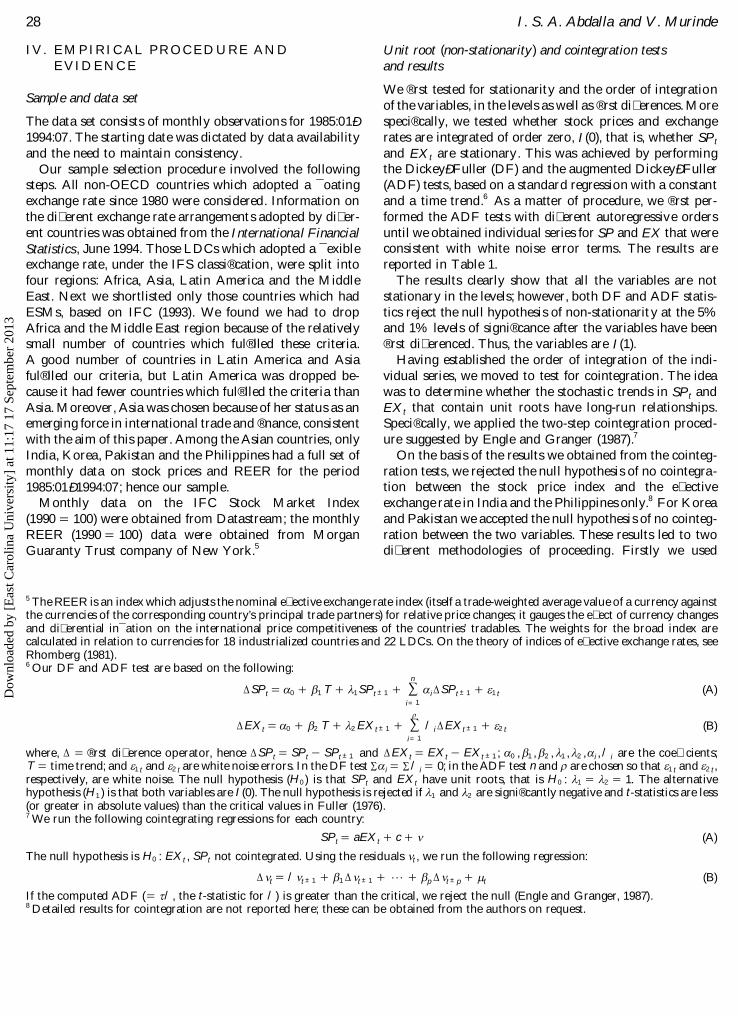
IV. EMPIRICAL PROCEDURE ANDEVIDENCE

Sample and data set

The data set consists of monthly observations for 1985:01 Ð1994:07. The starting date was dictated by data availabilityand the need to maintain consistency.

Our sample selection procedure involved the followingsteps. All non-OECD countries which adopted a ¯ oatingexchange rate since 1980 were considered. Information onthe di� erent exchange rate arrangements adopted by di� er-ent countries was obtained from the International FinancialStatistics, June 1994. Those LDCs which adopted a ¯ exibleexchange rate, under the IFS classi® cation, were split intofour regions: Africa, Asia, Latin America and the MiddleEast. Next we shortlisted only those countries which hadESMs, based on IFC (1993). We found we had to dropAfrica and the Middle East region because of the relativelysmall number of countries which ful® lled these criteria.A good number of countries in Latin America and Asiaful® lled our criteria, but Latin America was dropped be-cause it had fewer countries which ful® lled the criteria thanAsia. Moreover, Asia was chosen because of her status as anemerging force in international trade and ® nance, consistentwith the aim of this paper. Among the Asian countries, onlyIndia, Korea, Pakistan and the Philippines had a full set ofmonthly data on stock prices and REER for the period1985:01 Ð 1994:07; hence our sample.

Monthly data on the IFC Stock Market Index(1990 = 100) were obtained from Datastream; the monthlyREER (1990 = 100) data were obtained from MorganGuaranty Trust company of New York.5

Unit root (non-stationarity) and cointegration testsand results

We ® rst tested for stationarity and the order of integrationof the variables, in the levels as well as ® rst di� erences. Morespeci® cally, we tested whether stock prices and exchangerates are integrated of order zero, I(0), that is, whether SPt

and EXt are stationary. This was achieved by performingthe Dickey Ð Fuller (DF) and the augmented Dickey Ð Fuller(ADF) tests, based on a standard regression with a constantand a time trend.6 As a matter of procedure, we ® rst per-formed the ADF tests with di� erent autoregressive ordersuntil we obtained individual series for SP and EX that wereconsistent with white noise error terms. The results arereported in Table 1.

The results clearly show that all the variables are notstationary in the levels; however, both DF and ADF statis-tics reject the null hypothesis of non-stationarity at the 5%and 1% levels of signi® cance after the variables have been® rst di� erenced. Thus, the variables are I(1).

Having established the order of integration of the indi-vidual series, we moved to test for cointegration. The ideawas to determine whether the stochastic trends in SPt andEXt that contain unit roots have long-run relationships.Speci® cally, we applied the two-step cointegration proced-ure suggested by Engle and Granger (1987).7

On the basis of the results we obtained from the cointeg-ration tests, we rejected the null hypothesis of no cointegra-tion between the stock price index and the e� ectiveexchange rate in India and the Philippines only.8 For Koreaand Pakistan we accepted the null hypothesis of no cointeg-ration between the two variables. These results led to twodi� erent methodologies of proceeding. Firstly we used

28 I. S. A. Abdalla and V . MurindeD

ownl

oade

d by

[E

ast C

arol

ina

Uni

vers

ity]

at 1

1:17

17

Sept

embe

r 20

13

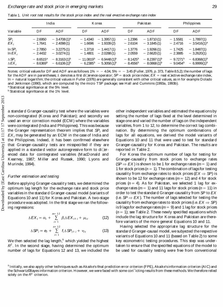
Table 1. Unit root test results for the stock price index and the real e¤ ective exchange rate index

India Korea Pakistan Philippines

Variable DF ADF DF ADF DF ADF DF ADF

SPt - 2.6950 - 3.4708 (1)a - 1.4340 - 1.3957 (1) - 1.2396 - 1.8710 (1) - 1.5581 - 1.7897(1)EXt - 1.7641 - 2.4098 (1) - 1.6696 - 1.9339 (2) - 2.6104 - 3.1845 (1) - 2.4716 - 3.5416(1)a

ln SPt - 2.7850 - 3.2275 (1) - 1.3718 - 1.4417 (1) - 1.3776 - 1.9266 (1) - 1.7425 - 1.8487(1)ln EXt - 2.4432 - 3.0274 (1) - 1.4801 - 2.0288 (1) - 2.0559 - 2.6620 (1) - 2.3885 - 3.2620(1)

D SPt - 8.6515a - 8.3163 (1)b - 11.0819b - 6.9448 (1)b - 8.1425b - 8.2397 (1)b - 9.7271b - 6.8368(1)b

D EXt - 8.6369b - 6.6106 (1)b - 6.2385b - 5.3058 (1)b - 8.4556b - 8.0868 (1)b - 9.0454b - 6.9999(1)b

Notes: critical values for DF and ADF are as follows: 1% = - 4.04, 5% = - 3.45 (Fuller, 1976, p. 373, Table 8.5.2); the number of lagsfor the ADF are in parentheses; D denotes a ® rst di� erence operator; SP = stock price index; EX = real e� ective exchange rate index,ln = natural logarithm; the critical values in Fuller (1976) are generally consistent with other critical values, as in for example Doladoand Jenkinson (1990), which are computed by the micro TSP package; see Hall and Cummins (1993a, 1993b).a Statistical signi® cance at the 5% level.b Statistical signi® cance at the 1% level.

9 Initially, we also apply other techniques such as Akaike’s ® nal prediction error criterion (FPE), Akaike’s information criterion (AIC) andthe Schwartz Ð Bayes information criterion. However, we were faced with some con¯ icting results from these methods. We therefore reliedsolely on the R2 criterion.

a standard Granger-causality test where the variables werenon-cointegrated (Korea and Pakistan); and secondly weused an error correction model (ECM) where the variableswere cointegrated (India and Philippines). This was becausethe Granger representation theorem implies that SPt andEXt may be generated by an ECM in the case of India andthe Philippines. Indeed, it has been con® rmed elsewherethat Granger-causality tests are misspeci® ed if they areapplied in a standard vector autoregressive form to di� er-enced data for cointegrated variables (MacDonald andKearney, 1987; Miller and Russek, 1990; Lyons andMurinde, 1994).

Further estimation and testing

Before applying Granger-causality tests, we determined theoptimum lag length for the exchange rate and stock pricevariables in the standard Granger-causal model (variants ofEquations 10 and 11) for Korea and Pakistan. A two-stageprocedure was adopted. In the ® rst stage we ran the follow-ing regressions:

D EXt = a 1 +m= 1 2

+i= 1

b i D EXt ± i + m 1 t (12)

D SP i = e2 +n= 1 2

+i= 1

fi D SPt ± i + n 2 t (13)

We then selected the lag length,9 which yielded the highestR2 . In the second stage, having determined the optimumnumber of lags for Equations 12 and 13, we included the

other independent variables and estimated the equations bysetting the number of lags ® xed at the level determined instage one and varied the number of lags on the independentvariables, from 1 to 12, to determine the correct lag combi-nation. By determining the optimum combinations oflags for all equations, we derived the model variants ofEquations 10 and 11 that were used to test for standardGranger-causality for Korea and Pakistan. The results arereported in Table 2.

For Korea the optimum number of lags for testing forGranger-causality from stock prices to exchange rates(SP Þ EX) is shown to be 1 for exchange rates (m = 1) and1 for stock prices (n = 1). The combination of lags for testingcausality from exchange rates to stock prices (EX Þ SP) isshown to be 12 for exchange rates (m = 12) and 4 for stockprices (n = 4). As for Pakistan, we selected 1 lag for ex-change rates (m = 1) and 11 lags for stock prices (n = 11) inorder to test the standard Granger-causality from SP to EX(i.e. SP Þ EX). The number of lags selected for testing thecausality from exchange rates to stock prices (i.e. EX Þ SP)is 9 lags for exchange rates (m = 9) and 1 lag for stock prices(n = 1); see Table 2. These newly speci® ed equations whichinclude the lag structure for Korea and Pakistan are there-fore variants of the more general Equations 10 and 11.

Having selected the appropriate lag structure for thestandard Granger-causal model, we subjected the respectivevariants of Equations 10 and 11 (based on Table 2) to somekey econometric testing procedures. This step was under-taken to ensure that the speci® ed equations of the model tobe used for causality testing were free from conventional

Exchange rate and stock price in emerging markets 29D

ownl

oade

d by

[E

ast C

arol

ina

Uni

vers

ity]

at 1

1:17

17

Sept

embe

r 20

13

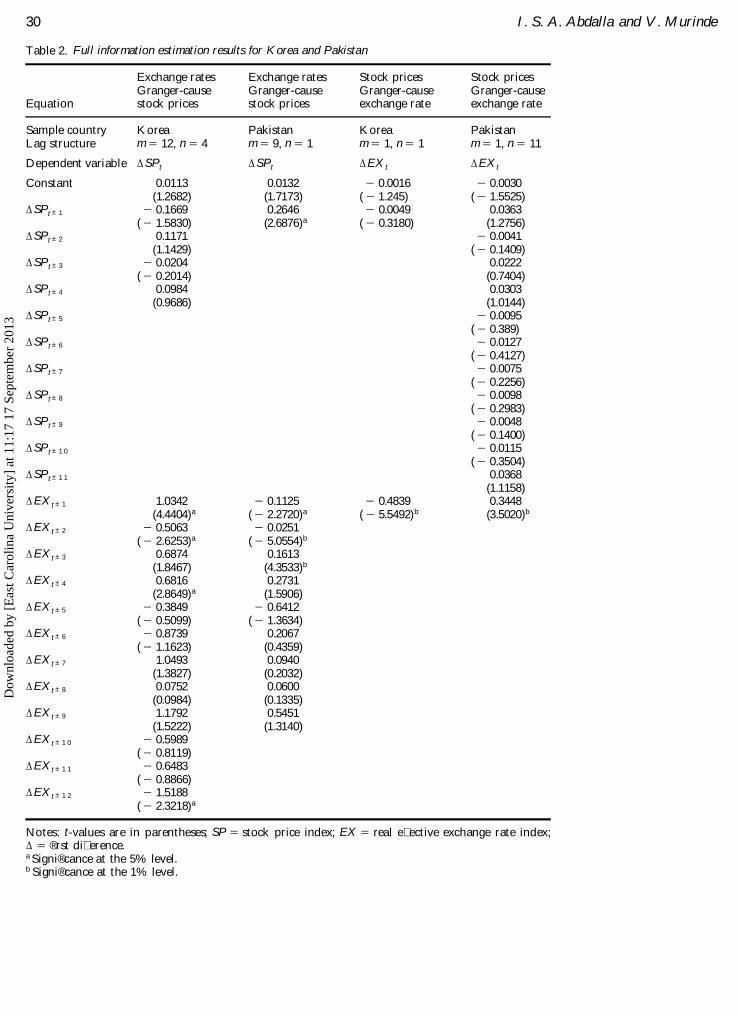
Table 2. Full information estimation results for Korea and Pakistan

Equation

Exchange ratesGranger-causestock prices

Exchange ratesGranger-causestock prices

Stock pricesGranger-causeexchange rate

Stock pricesGranger-causeexchange rate

Sample country Korea Pakistan Korea PakistanLag structure m = 12, n = 4 m = 9, n = 1 m = 1, n = 1 m = 1, n = 11

Dependent variable D SPt D SPt D EXt D EXt

Constant 0.0113 0.0132 - 0.0016 - 0.0030(1.2682) (1.7173) ( - 1.245) ( - 1.5525)

D SPt ± 1 - 0.1669 0.2646 - 0.0049 0.0363( - 1.5830) (2.6876)a ( - 0.3180) (1.2756)

D SPt ± 2 0.1171 - 0.0041(1.1429) ( - 0.1409)

D SPt ± 3 - 0.0204 0.0222( - 0.2014) (0.7404)

D SPt ± 4 0.0984 0.0303(0.9686) (1.0144)

D SPt ± 5 - 0.0095( - 0.389)

D SPt ± 6 - 0.0127( - 0.4127)

D SPt ± 7 - 0.0075( - 0.2256)

D SPt ± 8 - 0.0098( - 0.2983)

D SPt ± 9 - 0.0048( - 0.1400)

D SPt ± 1 0 - 0.0115( - 0.3504)

D SPt ± 1 1 0.0368(1.1158)

D EXt ± 1 1.0342 - 0.1125 - 0.4839 0.3448(4.4404)a ( - 2.2720)a ( - 5.5492)b (3.5020)b

D EXt ± 2 - 0.5063 - 0.0251( - 2.6253)a ( - 5.0554)b

D EXt ± 3 0.6874 0.1613(1.8467) (4.3533)b

D EXt ± 4 0.6816 0.2731(2.8649)a (1.5906)

D EXt ± 5 - 0.3849 - 0.6412( - 0.5099) ( - 1.3634)

D EXt ± 6 - 0.8739 0.2067( - 1.1623) (0.4359)

D EXt ± 7 1.0493 0.0940(1.3827) (0.2032)

D EXt ± 8 0.0752 0.0600(0.0984) (0.1335)

D EXt ± 9 1.1792 0.5451(1.5222) (1.3140)

D EXt ± 1 0 - 0.5989( - 0.8119)

D EXt ± 1 1 - 0.6483( - 0.8866)

D EXt ± 1 2 - 1.5188( - 2.3218)a

Notes: t-values are in parentheses; SP = stock price index; EX = real e� ective exchange rate index;D = ® rst di� erence.a Signi® cance at the 5% level.b Signi® cance at the 1% level.

30 I. S. A. Abdalla and V . MurindeD

ownl

oade

d by

[E

ast C

arol

ina

Uni

vers

ity]

at 1

1:17

17

Sept

embe

r 20

13

1 0 For Pakistan we corrected for heteroscedasticity by using the robust option that causes TSP to compute standard errors which areconsistent even in the presence of unknown heteroscedasticity (White, 1980; Hall and Cummins, 1993a, b).1 1 We calculated the Chow test based on the following:

F* =SSRp - (SSRp1 + SSRp2 )/k

(SSRp1 + SSRp2 )/(n1 + n2 - 2k)

where, SSRp = sum of square residual for the entire period; SSRp1 = sum of squared residual for period 1; SSRp2 = sum of squaredresidual for period 2; n1 = number of observation in period 1; n2 = number of observations in period 2; and k = the number of parameters.1 2 If the calculated F-statistic exceeds the critical value, H0 is rejected, otherwise H0 is accepted.

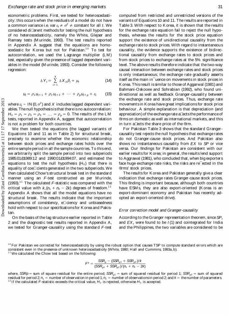
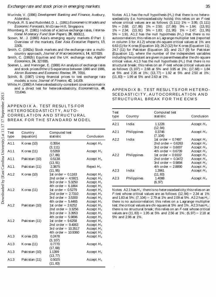
econometric problems. First, we tested for heteroscedasti-city: this occurs when the residuals of a model do not havea common variance i.e. var e t ¹ s 2 ¹ constant for all t. Weconsidered di� erent methods for testing the null hypothesisof no heteroscedasticity, namely the White, Glejser andRamsey tests (Murinde, 1993). The test results reportedin Appendix A suggest that the equations are homo-scedastic for Korea but not for Pakistan.1 0 To test forautocorrelation, we used the Lagrange multiplier (LM)test, especially given the presence of lagged dependent vari-ables in the model (Murinde, 1993). Consider the followingregression:

D Y t =k

+i= 1

D Xit b i + m t (14)

ut = r 1 ut ± 1 + r 2 ut ± 2 + ¼ + r p ut ± p + e t (15)

where e t ~ IN(0, s 2 ) and X includes lagged dependent vari-ables. The null hypothesis is that there is no autocorrelation:H0 = r 1 = r 2 = r 3 = ¼ = r p = 0. The results of the LMtests, reported in Appendix A, suggest that autocorrelationis not a problem for both countries.

We then tested the equations (the lagged variants ofEquations 10 and 11 as in Table 2) for structural break,precisely to examine whether the economic relationshipbetween stock prices and exchange rates holds over theentire sample period in all the sample countries. To this end,we arbitrarily split the sample period into two subperiods1985:01 Ð 1989:12 and 1990:01 Ð 1994:07, and estimated theequations to test the null hypothesis (H0 ) that there isequality of coe� cients generated in the two subperiods. Wethen calculated Chow’s structural break test in the standardmanner using an F-test constructed as per Murinde,(1993).1 1 The calculated F-statistic was compared with thecritical value with k, (n1 + n2 - 2k) degrees of freedom.1 2

Appendix A shows that all the model equations have nostructural break. The results indicate that the importantassumptions of consistency, e� ciency and unbiasednesshold with respect to our speci® cations for Korea and Pakis-tan.

On the basis of the lag structure earlier reported in Table2 and the diagnostic test results reported in Appendix A,we tested for Granger-causality using the standard F-test

computed from restricted and unrestricted versions of thevariants of Equations 10 and 11. The results are reported inTable 3. With respect to Korea, it is shown that the resultsfor the exchange rate equation fail to reject the null hypo-thesis, whereas the results for the stock price equationsupport the existence of unidirectional causality from theexchange rate to stock prices. With regard to instantaneouscausality, the evidence supports the existence of bidirec-tional causality from exchange rates to stock prices andfrom stock prices to exchange rates at the 5% signi® cancelevel. The above results therefore indicate that the two-waycausal interaction between exchange rates and stock pricesis only instantaneous; the exchange rate gradually assertsitself as the main in¯ uence on movements in stock prices inKorea. This result is similar to those of Aggarwal (1981) andBahmani-Oskooee and Sohrabian (1992), who found uni-directional as well as feedback Granger-causality betweenthe exchange rate and stock prices. Thus, exchange ratemovements in Korea have great implications for stock pricebehaviour. A simple explanation is that depreciation (andappreciation) of the exchange rate a� ects the performance of® rms on domestic as well as international markets, and thisin turn a� ects the share price of the ® rm.

For Pakistan Table 3 shows that the standard Granger-causality test rejects the null hypothesis that exchange ratesdo not Granger-cause stock prices. And Pakistan alsoshows no instantaneous causality from EX to SP or viceversa. Our ® ndings for Pakistan are consistent with ourearlier results for Korea; in general, the results lend supportto Aggrawal (1981), who concluded that, when big exportersface huge exchange rate risks, the risks are re¯ ected in the® rms’ stock prices.

The results for Korea and Pakistan generally give a clearindication that exchange rates Granger-cause stock prices.This ® nding is important because, although both countrieshave ESMs, they are also export-oriented (Korea is anexport-dominant economy and Pakistan has recently ad-opted an export-oriented drive).

Error correction model and Granger-causality

According to the Granger representation theorem, since SPt

and EXt were found to be I(1) and cointegrated for Indiaand the Philippines, the two variables are considered to be

Exchange rate and stock price in emerging markets 31D

ownl

oade

d by

[E

ast C

arol

ina

Uni

vers

ity]

at 1

1:17

17

Sept

embe

r 20

13

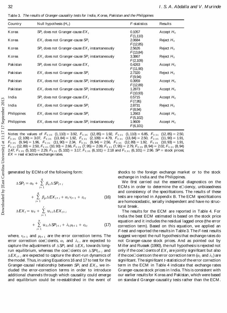
Table 3. The results of Granger-causality tests for India, Korea, Pakistan and the Philippines

Country Null hypothesis (H0 ) F-statistics Results

Korea SPt does not Granger-cause EXt 0.1057F(1,110)

Accept H0

Korea EXt does not Granger-cause SPt 2.0684F(12,85)

Reject H0

Korea SPt does not Granger-cause EXt instantaneously 2.5626F(13,84)

Reject H0

Korea EXt does not Granger-cause SPt instantaneously 3.3867F(2,109)

Reject H0

Pakistan SPt does not Granger-cause EXt 0.4263F(11,90)

Accept H0

Pakistan EXt does not Granger-cause SPt 2.7320F(9,94)

Reject H0

Pakistan EXt does not Granger-cause SPt instantaneously 0.3959F(12,89)

Accept H0

Pakistan EXt does not Granger-cause SPt instantaneously 1.2873F(10,93)

Accept H0

India SPt does not Granger-cause EXt 0.5715F(7,95)

Accept H0

India EXt does not Granger-cause SPt 2.8731F(8,94)

Reject H0

Philippines EXt does not Granger-cause SPt 1.2663F(5,102)

Accept H0

Philippines EXt does not Granger-cause SPt instantaneously 1.9609F(6,101)

Accept H0

Notes: the values of F0 . 0 5 (1, 110) = 3.92, F0 . 0 5 (12, 85) = 1.92, F0 . 0 1 (1, 110) = 6.85, F0 . 0 1 (12, 85) = 2.50,F0 . 0 5 (2, 109) = 3.07, F0 . 0 5 (13, 84) = 1.92, F0 . 0 1 (2, 109) = 4.79, F0 . 0 1 (13, 84) = 2.50, F0 . 0 5 (11, 90) = 1.91,F0 . 0 5 (9, 94) = 1.96, F0 . 0 1 (11, 90) = 2.34, F0 . 0 1 (9, 94) = 2.56, F0 . 0 5 (12, 89) = 1.92, F0 . 0 5 (10, 93) = 1.91,F0 . 0 1 (12, 89) = 2.50, F0 . 0 1 (10, 93) = 2.66, F0 . 0 5 (7, 95) = 2.09, F0 . 0 1 (7, 95) = 2.79, F0 . 0 5 (8, 94) = 2.02, F0 . 0 1 (8, 94)2.47, F0 . 0 5 (5, 102) = 2.29, F0 . 0 1 (5, 102) = 3.17, F0 . 0 5 (6, 101) = 2.18 and F0 . 0 1 (6, 101) = 2.96. SP = stock prices;EX = real e� ective exchange rates.

generated by ECMs of the following form:

D SPt = a 0 +q

+i= 1

b xi D SPt ± i

+q

+i= 1

b yi D EXt ± i + a 1 n t ± 1 + e 1 t (16)

D EXt = u 0 +r

+i= 1

u 1 i D EXt ± i

+h

+i= 1

u 2 i D SPt ± i + l 1 m t ± 1 + e 2 t (17)

where, n t ± 1 and m t ± 1 are the error correction terms. Theerror correction coe� cients, a 1 and l 1 , are expected tocapture the adjustments of D SPt and D EXt towards long-run equilibrium, whereas the coe� cients on D SPtt ± i andD EXt ± i are expected to capture the short-run dynamics ofthe model. Thus, in using Equations 16 and 17 to test for theGranger-causal relationship between SPt and EXt , we in-cluded the error-correction terms in order to introduceadditional channels through which causality could emergeand equilibrium could be re-established in the event of

shocks to the foreign exchange market or to the stockexchange in India and the Philippines.

We ® rst carried out the essential diagnostics on theECMs in order to determine the e� ciency, unbiasednessand consistency of the speci® cations. The results of thesetests are reported in Appendix B. The ECM speci® cationsare homoscedastic, serially independent and have no struc-tural break.

The results for the ECM are reported in Table 4. ForIndia the best ECM estimated is based on the stock priceequation and it includes the residual lagged once (the errorcorrection term). Based on this equation, we applied anF-test and reported the results in Table 3. The F-test resultssuggest we reject the null hypothesis that exchange rates donot Granger-cause stock prices. And as pointed out byMiller and Russek (1990), the null hypothesis is rejected notonly if the coe� cients of EXt are jointly signi® cant but alsoif the coe� cients on the error correction term (a 1 and l 1 ) aresigni® cant. The signi® cant t-statistics of the error correctionterm in the ECM in Table 4 indicate that exchange ratesGranger-cause stock prices in India. This is consistent withour earlier results for Korea and Pakistan, which were basedon standard Granger-causality tests rather than the ECM.

32 I. S. A. Abdalla and V . MurindeD

ownl

oade

d by

[E

ast C

arol

ina

Uni

vers

ity]

at 1

1:17

17

Sept

embe

r 20

13

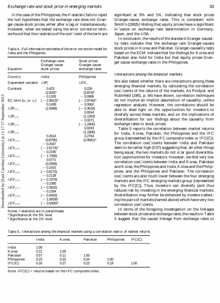
Table 5. Interactions among the Þ nancial markets using a correlation matrix of market returns

India Korea Pakistan Philippines IFC(C)

India 1.00Korea 0.21 1.00Pakistan 0.57 0.11 1.00Philippines 0.23 0.32 0.24 1.00IFC(C) 0.16 0.27 0.22 0.19 1.00

Note: IFC(C) = returns based on the IFC composite index.

Table 4. Full information estimates of the error correction model forIndia and the Philippines

Equation

Exchange ratesGranger-causestock prices

Stock pricesGranger-causeexchange rates

Country India Philippines

Dependent variable D SPt D EXt

Constant 0.423 0.226(2.920)a (3.874)b

- 0.1333 - 0.0995EC term (a 1 or l 1 ) ( - 2.9913)a ( - 2.9740)a

0.1439 - 0.0062D SPt ± 1 (1.5068) ( - 0.3018)

0.0244D SPt ± 2 (1.1263)

- 0.0271D SPt ± 3 ( - 1.2400)

0.0243D SPt ± 4 (1.1906)

0.2614 0.2764D EXt ± 1 (0.8790) (2.9581)a

- 0.2047D EXt ± 2 ( - 2.6774)a

- 0.2190D EXt ± 3 ( - 1.7266)

0.0771D EXt ± 4 (0.2559)

- 0.1915D EXt ± 5 ( - 0.6275)

- 0.2128D EXt ± 6 ( - 0.7079)

- 0.1095D EXt ± 7 ( - 0.3632)

- 0.1354D EXt ± 8 ( - 0.4493)

- 1.08330D EXt ± 9 ( - 3.6306)b

Notes: t-statistics are in parentheses.a Signi® cance at the 5% level.b Signi® cance at the 1% level.

In the case of the Philippines, the F-statistic fails to rejectthe null hypothesis that the exchange rate does not Gran-ger-cause stock prices, either after a lag or instantaneously .However, when we tested using the error correction term,we found that the t-statistics of the coe� cient of the term are

signi® cant at 5% and 1%, indicating that stock pricesGranger-cause exchange rates. This is consistent withSmith’s (1992b) ® nding that equity prices have a signi® cantin¯ uence on exchange rate determination in Germany,Japan, and the USA.

In conclusion, the results of the standard Granger-causal-ity tests indicate that the exchange rate Granger-causesstock prices in Korea and Pakistan. Granger-causality testsbased on the ECM indicate that the ® ndings for Korea andPakistan also hold for India but that equity prices Gran-ger-cause exchange rates in the Philippines.

Interactions among the Þ nancial markets

We also tested whether there are interactions among theseemerging ® nancial markets, by calculating the correlationcoe� cients of the returns of the markets. As Pindyck andRubinfeld (1991, p. 64) have shown, correlation techniquesdo not involve an implicit assumption of causality, unlikeregression analysis. However, the correlations should beable to shed light on the opportunities for investors todiversify across these markets, and on the implications ofdiversi® cation for our ® ndings about the causality fromexchange rates to stock prices.

Table 5 reports the correlation between market returnsfor India, Korea, Pakistan, the Philippines and the IFCgroup (represented by the IFC composite index or IFC(C)).The correlation coe� cients between India and Pakistanseem to be rather high (0.57) suggesting that, all other thingsbeing equal, the two markets do not o� er good diversi ® ca-tion opportunities for investors. However, we ® nd very lowcorrelation coe� cients between India and Korea, Pakistanand Korea, the Philippines and India, Korea and the Philip-pines, and the Philippines and Pakistan. The correlationcoe� cients are also much lower between the four emergingmarkets and the IFC emerging markets group (representedby the IFC(C)). Thus, investors can diversify (and thusreduce) risk by investing in the emerging ® nancial markets;diversi® cation may further be enhanced by investors select-ing the pairs of markets (named above) which have very lowcorrelation coe� cients.

In terms of the foregoing investigation on the linkagesbetween stock prices and exchange rates, the results in Table5 suggest that the causal linkage from exchange rates to

Exchange rate and stock price in emerging markets 33D

ownl

oade

d by

[E

ast C

arol

ina

Uni

vers

ity]

at 1

1:17

17

Sept

embe

r 20

13

1 3 Lutkepohl and Reimers (1992) propose and implement a consistent procedure for Granger-causality testing. First, they perform ADFwith di� erent autoregressive orders. Second, they apply the order selection criterion (SC) to unrestricted VAR in order to determine the laglength. Third, they conduct the Johansen test for cointegration. Fourth, they do the diagnostic tests. Finally, they perform Granger-causality inference.

stock prices is likely to be independent of the markets, asthese markets do not exhibit very high comovements. Theexceptions are India and Pakistan, two markets which maybe related in terms of the causal linkage from exchange ratesto stock prices.

V. SUMMARY AND CONCLUSION

This paper sheds lights on the linkages between exchangerates and stock prices in some emerging markets. Somerecent econometric techniques are applied to a BVARmodel of stock prices and exchange rates in order to test forGranger-causality between the two variables. Essentially,we perform the ADF tests with di� erent autoregressiveorders until we obtain individual series for SP and EX thatare consistent with white noise error terms. Having estab-lished the order of integration of the individual series,we move to test for cointegration using the two-stepEngle Ð Granger procedure. The results suggest that we haveto proceed with a standard VAR for Korea and Pakistan,and an error correction model (ECM) for India and thePhilippines. Taking the standard VAR model, we determinethe optimum lag length of the bivariate VAR (BVAR), thencarry out diagnostics on the resulting equations, proceedingto test for inference of Granger-causality with these equa-tions for Korea and Pakistan. And taking the ECM wedetermine the optimum lag length of the ECM equations,then carry out diagnostics on the resulting equations, pro-ceeding to test for inference of Granger-causality with theseequations for India and the Philippines.

Among the ® ndings of interest, exchange rates Granger-cause stock prices in Korea, Pakistan and India, whereasstock prices Granger-cause exchange rates in the Philip-pines. Not only is the evidence on the causal in¯ uence ofexchange rates on stock prices strong, it is also consistentwith some earlier research based on developed economies,instead of the emerging market economies we investigate inthis paper. The main implications are that, in the case ofGranger-causality from exchange rates to stock prices,changes in exchange rates a� ect ® rms’ exports and ultimate-ly a� ect stock prices. Thus, in terms of policy relevance, the® ndings of this paper suggest that the respective govern-ments of these emerging markets should well be cautious intheir implementation of exchange rate policies, since theyhave rami® cations for the budding stock markets. A promis-ing way to proceed in further empirical investigation is touse a uni® ed framework’ for Granger-causal testing, re-cently suggested by Lutkepohl and Reimers (1992).1 3

ACKNOWLEDGEMENTS

We thank, without implication, Morgan Guaranty TrustCompany of New York for giving us REER data, and ananonymous referee of this journal for constructive com-ments on a previous draft of this paper.

REFERENCES

Aggarwal , R. (1981) Exchange rates and stock prices: a study of theUS capital markets under ¯ oating exchange rates, AkronBusiness and Economic Review, 12, 7 Ð 12.

Bahmani-Oskooee, M. and Sohrabian, A. (1992) Stock prices andthe e� ective exchange rate of the dollar, Applied Economics,24, 459 Ð 64.

Divecha, A. B., Drach, J. and Stefek, D. (1992) Emerging markets:a quantitative perspective, Journal of Portfolio Management,19, 41 Ð 50.

Dolado, J. J. and Jenkinson, T. (1990) Co-integration and unitroots, Journal of Economic Surveys, 4, 249 Ð 71.

Engle, R .F. and Granger, C. W. (1987) Co-integration: representa-tion, estimation, and testing, Econometrica , 55, 251 Ð 76.

Fuller, W. (1976) Introduction to Statistical T ime Series, Wiley,New York.

Granger, C. W. (1969) Investigating causal relations by econometricmodels and cross-spectral methods, Econometrica , 37, 424 Ð 39.

Hall, B. and Cummins, C. (1993a), T ime Series Processor, V ersion4.2, Users Guide, TSP International, New York.

Hall, B. and Cummins, C. (1993b), Time Series Processor, V ersion4.2, Reference Manual, TSP International, New York.

Hartmann, M. A. and Khambata, D. (1993) Emerging stock mar-kets investment and strategies of the future, The ColumbiaJournal of W orld Business, 28, 83 Ð 104.

IFC (1993) Emerging Stock Markets Factbook, InternationalFinance Corporation, Washington DC.

Jorion, P. (1990) The exchange-rate exposure of US multina-tionals, Journal of Business, 63, 331 Ð 45.

Loudon, G. (1993) The foreign exchange operating exposure ofAustralian stocks, Accounting and Finance, 33, 19 Ð 32.

Lutkepohl, H. and Reimers, H. (1992) Granger-causality in coin-tegrated VAR processes: the case of the term structure, Eco-nomics L etters, 40, 263 Ð 8.

Lyons, S. E. and Murinde, V. (1994) Cointegration and Grangercausality testing of hypothesis on supply leading and demandfollowing ® nance, Economic Notes, 23, 17 Ð 36.

Ma, C. K. and Kao, G. W. (1990) On exchange rate changes andstock price reactions, Journal of Business Finance and Ac-counting, 17, 441 Ð 9.

MacDonald, R. and Kearney, C. (1987) On the speci® cation ofGranger causality tests using the cointegration methodology,Economic L etters, 25, 149 Ð 53.

Miller, S. M. and Russek, F. S. (1990) Co-integration and errorcorrection models: the temporal causality between governmenttaxes and spending, Southern Economic Journal, 57, 221 Ð 9.

Murinde, V. (1993) Macroeconomic Policy Modelling for Develop-ing Countries, Avebury, Aldershot.

34 I. S. A. Abdalla and V . MurindeD

ownl

oade

d by

[E

ast C

arol

ina

Uni

vers

ity]

at 1

1:17

17

Sept

embe

r 20

13

Murinde, V. (1996) Development Banking and Finance, Avebury,Aldershot.

Pindyck, R. S. and Rubinfeld, D. L. (1991) Econometric Models andEconomic Forecasts, McGraw-Hill, Singapore.

Rhomberg, R. (1981) Indices of e� ective exchange rates, Interna-tional Monetary Fund Sta¤ Papers, 28, 88 Ð 111.

Scown, M. J. (1990) Asia’s emerging equity markets Ð Part 1:Overview of the markets, East Asia Executive Reports, 13,22 Ð 5.

Smith, C. (1992a) Stock markets and the exchange rate: a multi-country approach, Journal of Macroeconomics, 14, 607 Ð 29.

Smith, C. (1992b) Equities and the UK exchange rate, AppliedEconomics, 24, 327 Ð 35.

Soenen, L. and Hennigar, E. (1988) An analysis of exchange ratesand stock prices Ð the US experience between 1980 and 1986,Akron Business and Economic Review, 19, 7 Ð 16.

Solnik, B. (1987) Using ® nancial prices to test exchange ratemodels: a note, Journal of Finance, 42, 141 Ð 9.

White, H. (1980) A heteroskedasticity-consistent covariance matrixand a direct test for heteroskedasticity, Econometrica , 48,721 Ð 46.

APPENDIX A. TEST RESULTS FORHETEROSCEDASTICITY, AUTO-CORRELATION AND STRUCTURALBREAK FOR THE STANDARD MODEL

Testtype

Country(equation)

Computed teststatistic Conclusion

A1.1 Korea (10) 0.3554(3, 111)

Accept H0

A1.1 Korea (11) 0.5359(17, 86)

Accept H0

A1.1 Pakistan (10) 0.5138(13, 91)

Accept H0

A1.1 Pakistan (11) 2.3875(11, 95)

Reject H0

A1.2 Korea (10) 1st order = 0.11632nd order = 4.59213rd order = 5.32504th order = 6.1864

Accept H0

Accept H0

Accept H0

Accept H0

A1.2 Korea (11) 1st order = 0.52792nd order = 2.73103rd order = 3.53004th order = 5.4465

Accept H0

Accept H0

Accept H0

Accept H0

A1.2 Pakistan (10) 1st order = 2.62522nd order = 3.32563rd order = 3.39534th order = 5.9896

Accept H0

Accept H0

Accept H0

Accept H0

A1.2 Pakistan (11) 1st order = 9.62582nd order = 9.40633rd order = 10.35174th order = 10.9360

Accept H0

Accept H0

Accept H0

Accept H0

A1.3 Korea (10) 0.2478(3, 107)

Accept H0

A1.3 Korea (11) 0.7770(17, 68)

Accept H0

A1.3 Pakistan (10) 1.1399(13, 77)

Accept H0

A1.3 Pakistan (11) 0.5025(11, 83)

Accept H0

Notes: A1.1 has the null hypothesis (H0 ) that there is no hetero-scedasticity (i.e. homoscedasticity holds); this relies on an F-testwhose critical values are as follows: (3, 111) 1% = 3.95; (3, 111)5% = 2.68; (17, 86) 1% = 2.50; (17, 86) 5% = 1.84; (13, 91)1% = 2.34; (13, 91) 5% = 1.83; (11, 95) 1% = 2.47; (11, 95)5% = 1.91. A1.2 has the null hypothesis (H0 ) that there is noautocorrelation; this relies on a Lagrange multiplier test (reportedin column 3 for A1.2) whose chi-square critical values at 1% are6.63 (1) for Korea (Equation 10); 26.2 (12) for Korea (Equation 11);24.7 (11) for Pakistan (Equation 10); and 21.7 (9) for Pakistan(Equation 11), where the number of the independent variablesincluding the constant are given in parentheses after the chi-squarecritical value. A1.3 has the null hypothesis (H0 ) that there is nostructural break; this relies on an F-test whose critical values areas follows: (3, 107) = 2.68 at 5% and 3.95 at 1%; (17, 68) = 1.84at 5% and 2.35 at 1%; (13, 77) = 1.92 at 5% and 2.50 at 1%;(11, 83) = 1.99 at 5% and 2.63 at 1%.

APPENDIX B: TEST RESULTS FOR HETERO-SCEDASTICITY, AUTOCORRELATION ANDSTRUCTURAL BREAK FOR THE ECMS

Testtype Country

Computed teststatistic Conclusion

A2.1 India 1.1228(12, 94)

Accept H0

A2.1 Philippines 0.3746(7, 104)

Accept H0

A2.2 India 1st order = 0.74972nd order = 0.62633rd order = 0.60074th order = 0.6739

Accept H0

Accept H0

Accept H0

Accept H0

A2.2 Philippines 1st order = 0.91022nd order = 0.34723rd order = 0.98944th order = 2.8890

Accept H0

Accept H0

Accept H0

Accept H0

A2.3 India 1.3961(11, 83)

Accept H0

A2.3 Philippines 1.4088(6, 97)

Accept H0

Notes: A2.1 has H0 : there is no heteroscedasticity; this relies on anF-test whose critical values are as follows: (12, 94) = 2.34 at 1%and 1.83 at 5%; (7, 104) = 2.79 at 1% and 2.09 at 5%. A2.2 has H0 :there is no autocorrelation; this relies on a Lagrange multipliertest; the critical values are chi-square at 5% and 1%. A2.3 has H0 :there is no structural break; this relies on an F-test whose criticalvalues are (11, 83) = 1.95 at 5% and 2.56 at 1%; (6, 97) = 2.18 at5% and 2.96 at 1%.

.

Exchange rate and stock price in emerging markets 35D

ownl

oade

d by

[E

ast C

arol

ina

Uni

vers

ity]

at 1

1:17

17

Sept

embe

r 20

13