© 2002 Agilent Technologies - Used with Permission

Everything you've always wanted to know about Hot-S22 (but we're afraid to ask)

Jan Verspecht

Jan Verspecht bvba

Gertrudeveld 151840 SteenhuffelBelgium

email: contact@janverspecht.comweb: http://www.janverspecht.com

Slides presented at the WorkshopIntroducing New Concepts in Nonlinear Network Design

(International Microwave Symposium 2002)

Everything you’ve always wanted to know about

“Hot-S22”(but were afraid to ask)

Jan Verspecht

Agilent Technologies

2

Purpose

• Convince people of a better “Hot S22”

• Show that technology is fun (sometimes)

3

Outline

• Introduction: What is “Hot S22” ?

• Getting and interpreting experimental data

• Confront classic approaches with data

• Derivation of the extended “Hot S22” theory

• Confront extended “Hot S22” with data

• Conclusion

4

What is “Hot S22” ?

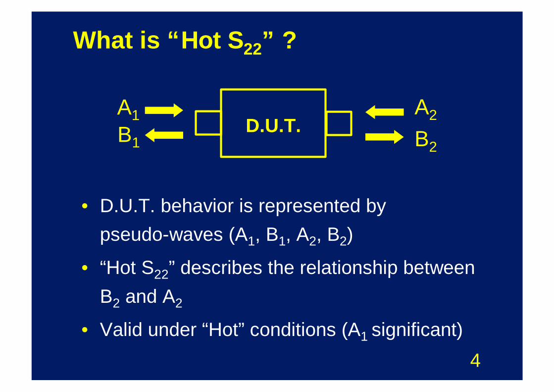
• D.U.T. behavior is represented by pseudo-waves (A1, B1, A2, B2)

• “Hot S22” describes the relationship between B2 and A2

• Valid under “Hot” conditions (A1 significant)

D.U.T.A1 A2B1 B2

5

Experimental investigation

• Take a real life D.U.T. (CDMA RFIC amplifier)

• Apply an A1 signal

• Apply a set of A2’s

• Look at the corresponding B2’s

• Mathematically describe the relationship between the A2’s and B2’s

• Repeat for different A1’s

6

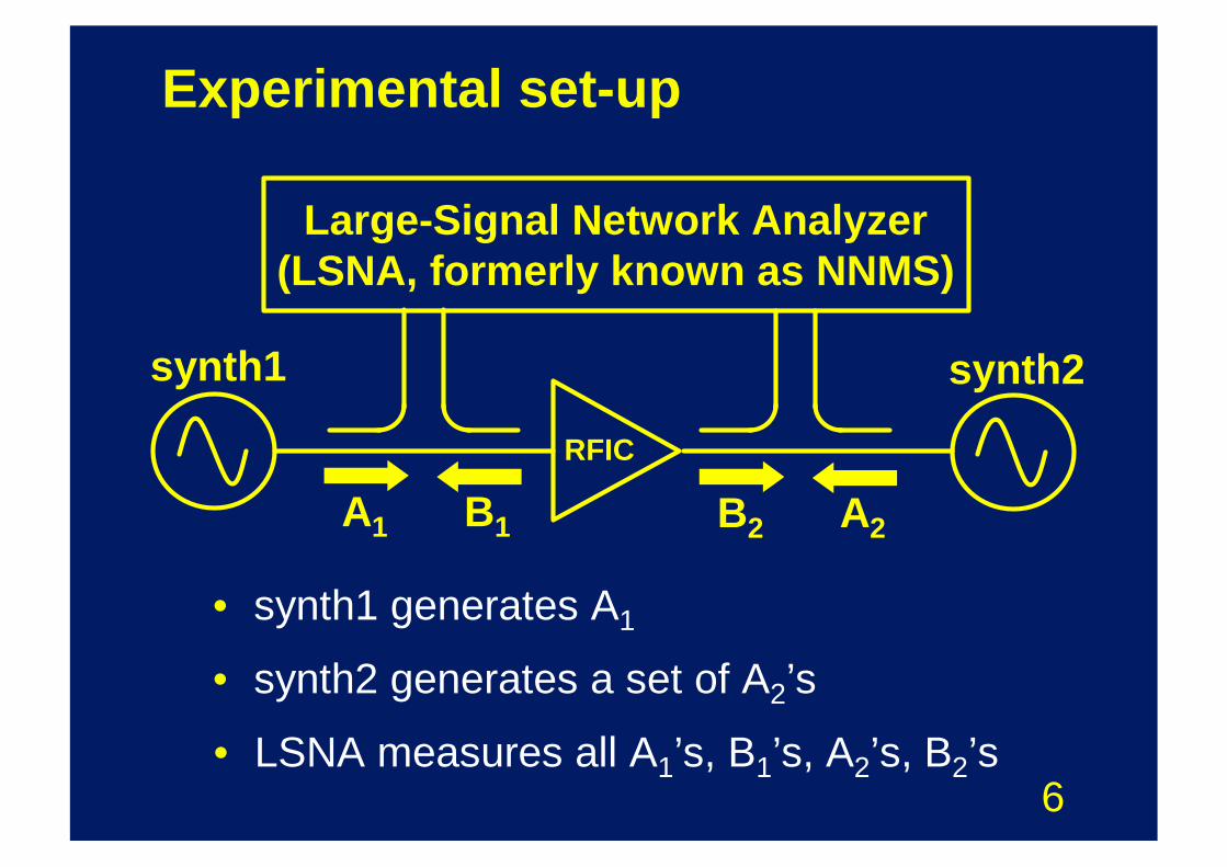
Experimental set-up

Large-Signal Network Analyzer(LSNA, formerly known as NNMS)

RFIC

A1 B1 B2 A2

synth2synth1

• synth1 generates A1

• synth2 generates a set of A2’s

• LSNA measures all A1’s, B1’s, A2’s, B2’s

7

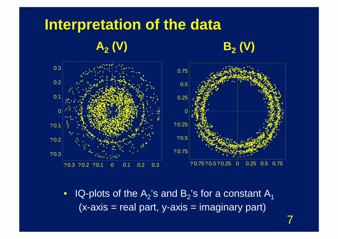
Interpretation of the data

? 0.3 ? 0.2 ? 0.1 0 0.1 0.2 0.3

? 0.3

? 0.2

? 0.1

0

0.1

0.2

0.3

? 0.75 ? 0.5 ? 0.25 0 0.25 0.5 0.75

? 0.75

? 0.5

? 0.25

0

0.25

0.5

0.75

A2 (V) B2 (V)

• IQ-plots of the A2’s and B2’s for a constant A1

(x-axis = real part, y-axis = imaginary part)

8

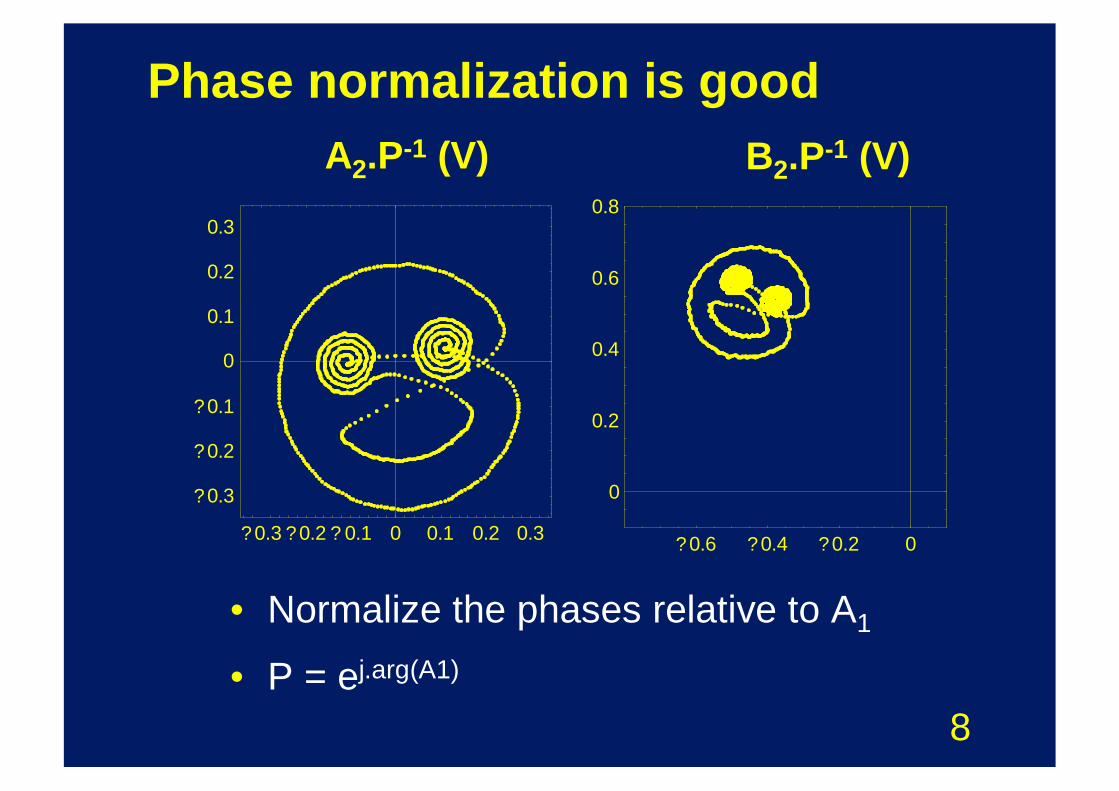
Phase normalization is good

• Normalize the phases relative to A1

• P = ej.arg(A1)

? 0.3 ? 0.2 ? 0.1 0 0.1 0.2 0.3

? 0.3

? 0.2

? 0.1

0

0.1

0.2

0.3

? 0.6 ? 0.4 ? 0.2 0

0

0.2

0.4

0.6

0.8

A2.P-1 (V) B2.P-1 (V)

9

? 1.25 ? 1 ? 0.75 ? 0.5 ? 0.25 0

0

0.25

0.5

0.75

1

1.25

1.5

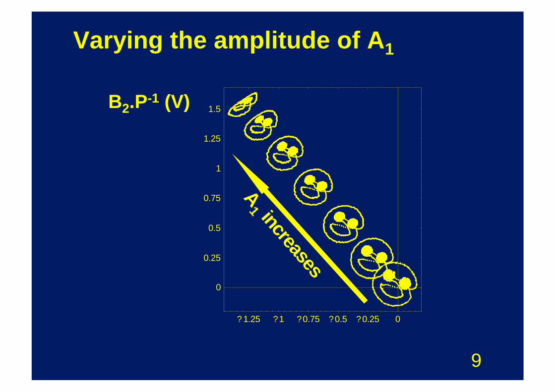
Varying the amplitude of A1

B2.P-1 (V)

A1 increases

10

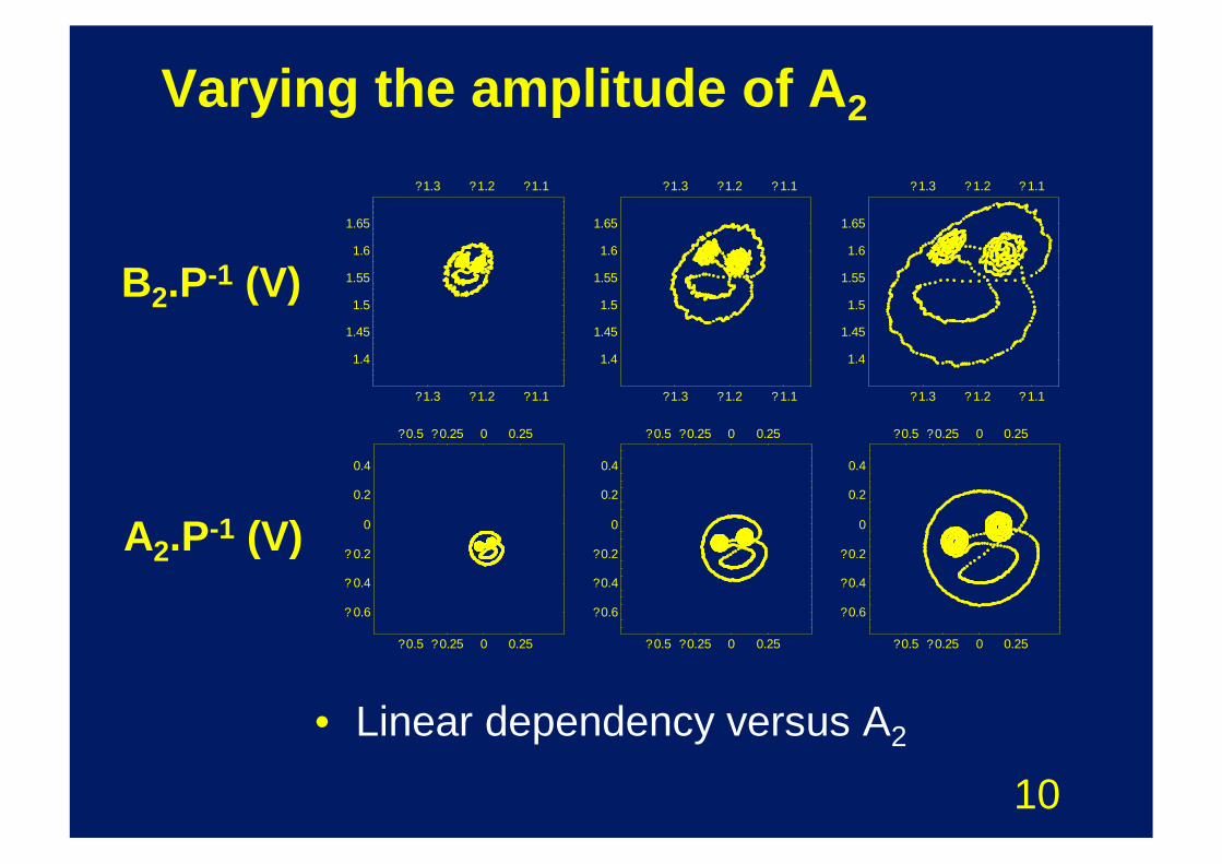
Varying the amplitude of A2

• Linear dependency versus A2

? 0.5 ? 0.25 0 0.25

? 0.6

? 0.4

? 0.2

0

0.2

0.4

? 0.5 ? 0.25 0 0.25

? 0.5 ? 0.25 0 0.25

? 0.6

? 0.4

? 0.2

0

0.2

0.4

? 0.5 ? 0.25 0 0.25

? 0.5 ? 0.25 0 0.25

? 0.6

? 0.4

? 0.2

0

0.2

0.4

? 0.5 ? 0.25 0 0.25

? 1.3 ? 1.2 ? 1.1

1.4

1.45

1.5

1.55

1.6

1.65

? 1.3 ? 1.2 ? 1.1

? 1.3 ? 1.2 ? 1.1

1.4

1.45

1.5

1.55

1.6

1.65

? 1.3 ? 1.2 ? 1.1

? 1.3 ? 1.2 ? 1.1

1.4

1.45

1.5

1.55

1.6

1.65

? 1.3 ? 1.2 ? 1.1

B2.P-1 (V)

A2.P-1 (V)

11

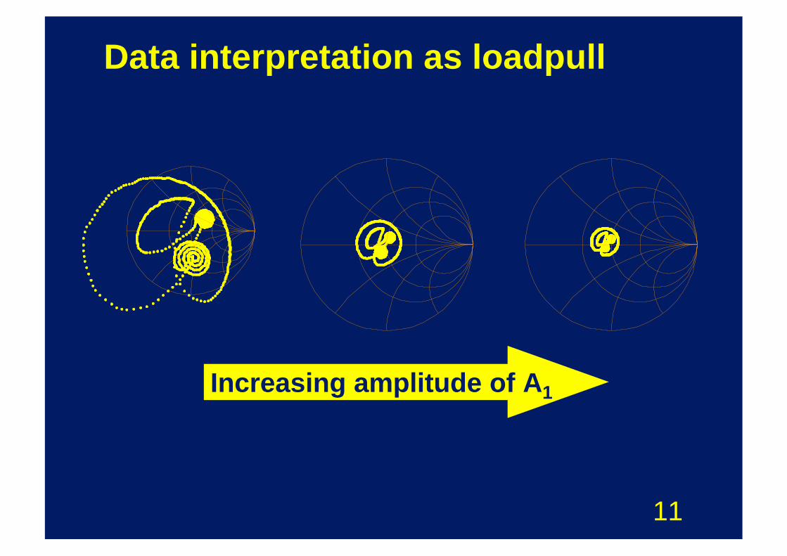
Data interpretation as loadpull

Increasing amplitude of A1

12

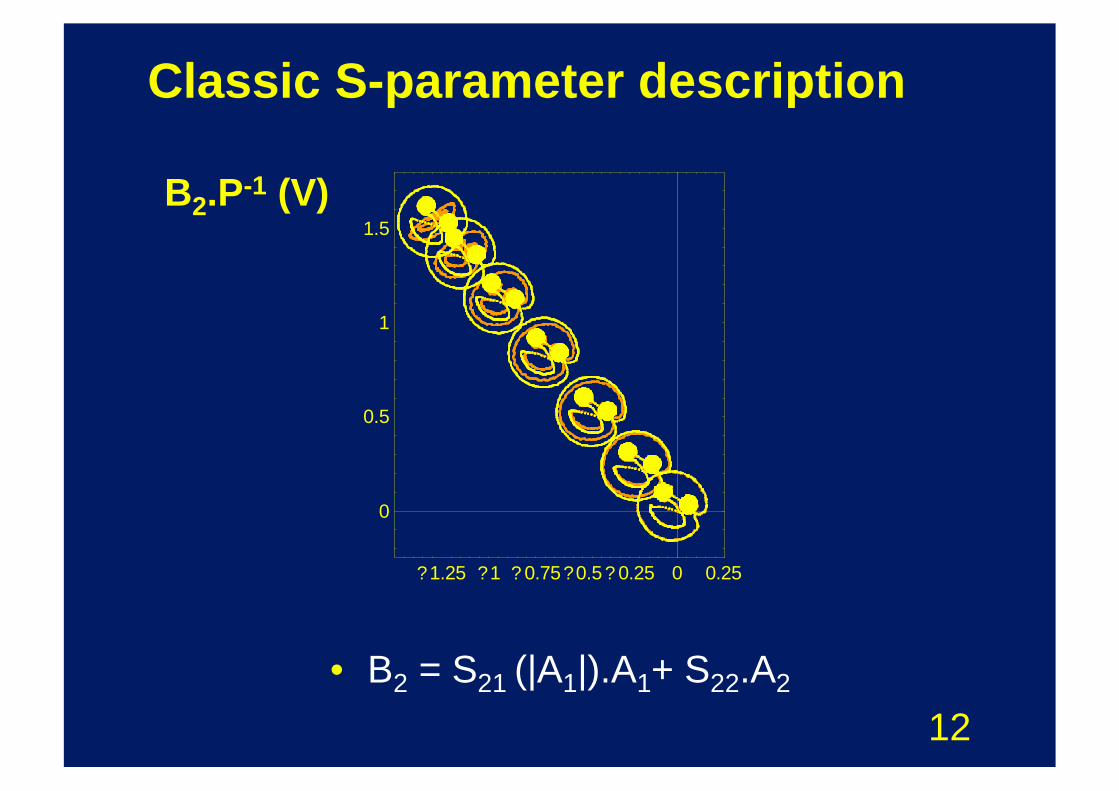
Classic S-parameter description

• B2 = S21 (|A1|).A1+ S22.A2

? 1.25 ? 1 ? 0.75 ? 0.5 ? 0.25 0 0.25

0

0.5

1

1.5B2.P-1 (V)

13

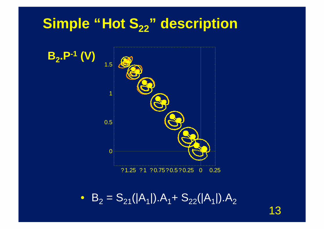
Simple “Hot S22” description

• B2 = S21(|A1|).A1+ S22(|A1|).A2

? 1.25 ? 1 ? 0.75 ? 0.5 ? 0.25 0 0.25

0

0.5

1

1.5B2.P-1 (V)

14

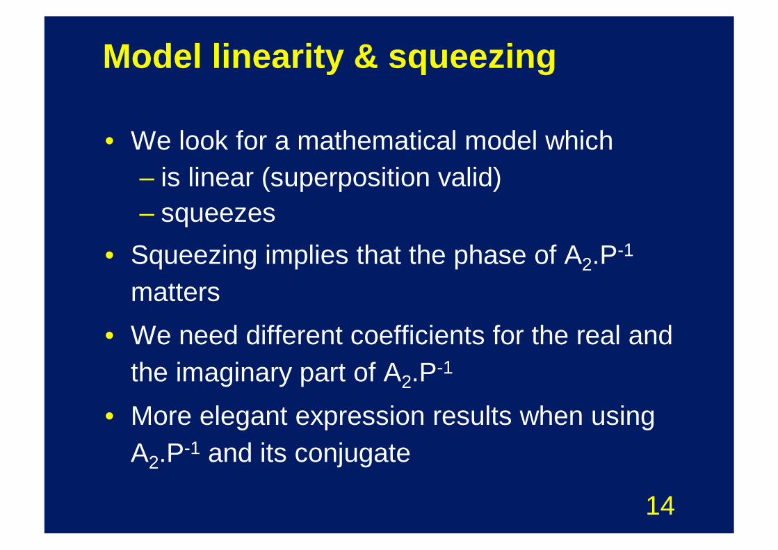
Model linearity & squeezing

• We look for a mathematical model which– is linear (superposition valid)– squeezes

• Squeezing implies that the phase of A2.P-1

matters

• We need different coefficients for the real and the imaginary part of A2.P-1

• More elegant expression results when using A2.P-1 and its conjugate

15

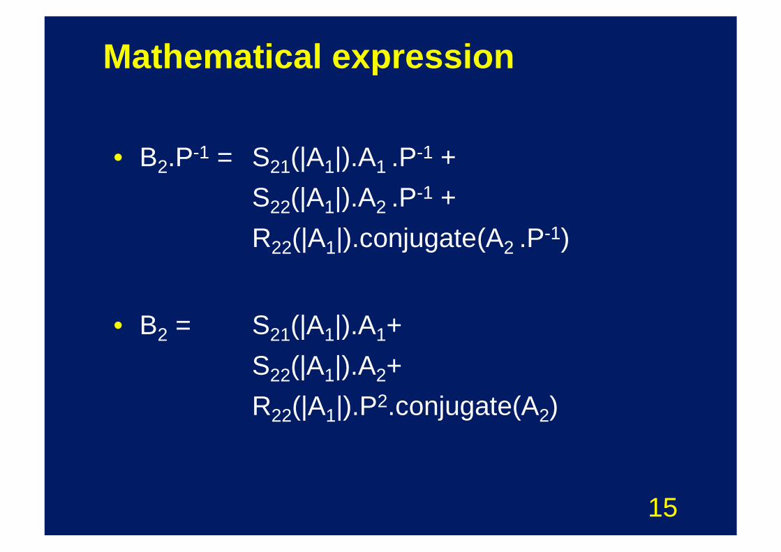
Mathematical expression

• B2.P-1 = S21(|A1|).A1 .P-1 + S22(|A1|).A2 .P-1 + R22(|A1|).conjugate(A2 .P-1)

• B2 = S21(|A1|).A1+S22(|A1|).A2+ R22(|A1|).P2.conjugate(A2)

16

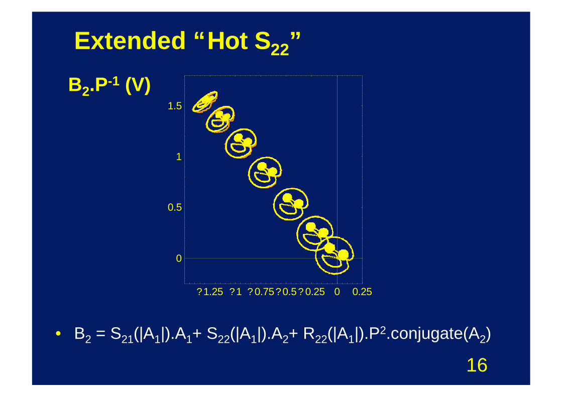
Extended “Hot S22”

• B2 = S21(|A1|).A1+ S22(|A1|).A2+ R22(|A1|).P2.conjugate(A2)

? 1.25 ? 1 ? 0.75 ? 0.5 ? 0.25 0 0.25

0

0.5

1

1.5

B2.P-1 (V)

17

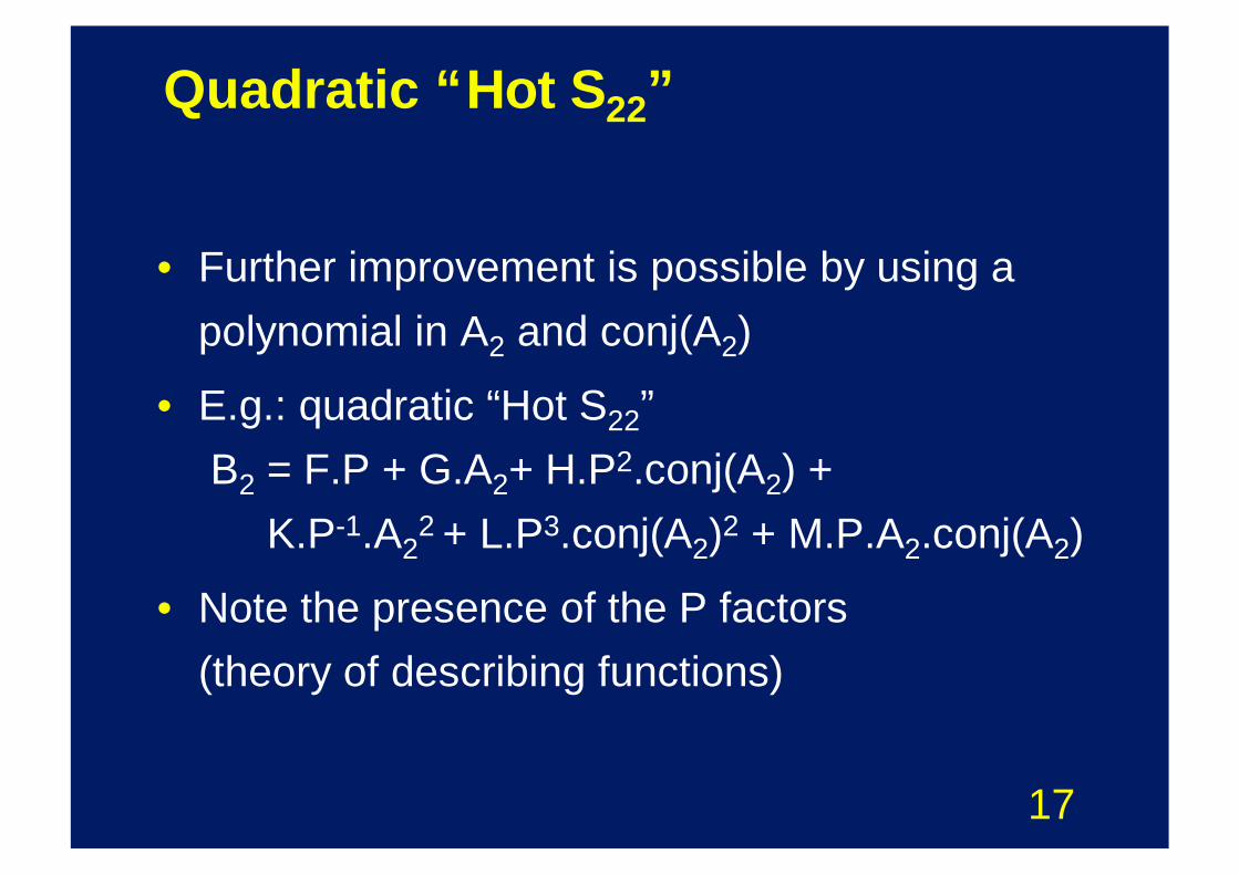
Quadratic “Hot S22”

• Further improvement is possible by using a polynomial in A2 and conj(A2)

• E.g.: quadratic “Hot S22”B2 = F.P + G.A2+ H.P2.conj(A2) +

K.P-1.A22 + L.P3.conj(A2)2 + M.P.A2.conj(A2)

• Note the presence of the P factors(theory of describing functions)

18

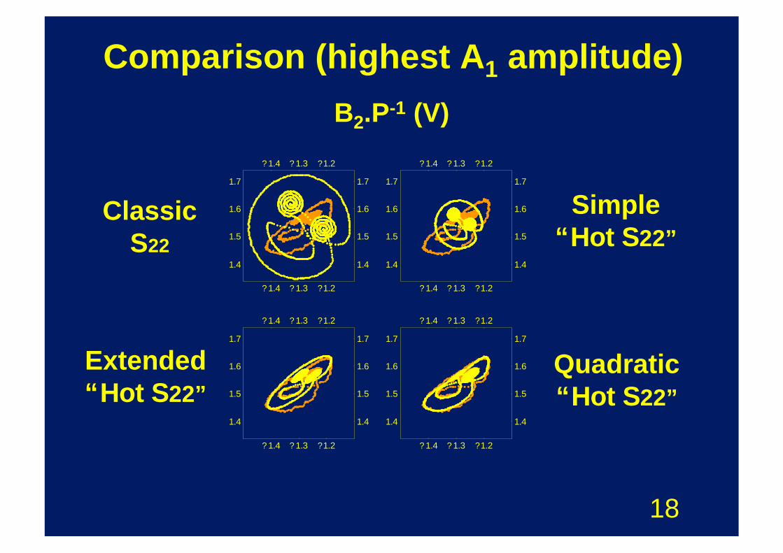
Comparison (highest A1 amplitude)

? 1.4 ? 1.3 ? 1.2

1.4

1.5

1.6

1.7

? 1.4 ? 1.3 ? 1.2

1.4

1.5

1.6

1.7

? 1.4 ? 1.3 ? 1.2

1.4

1.5

1.6

1.7

? 1.4 ? 1.3 ? 1.2

1.4

1.5

1.6

1.7

? 1.4 ? 1.3 ? 1.2

1.4

1.5

1.6

1.7

? 1.4 ? 1.3 ? 1.2

1.4

1.5

1.6

1.7

? 1.4 ? 1.3 ? 1.2

1.4

1.5

1.6

1.7

? 1.4 ? 1.3 ? 1.2

1.4

1.5

1.6

1.7

B2.P-1 (V)

ClassicS22

Simple“Hot S22”

Extended“Hot S22”

Quadratic“Hot S22”

19

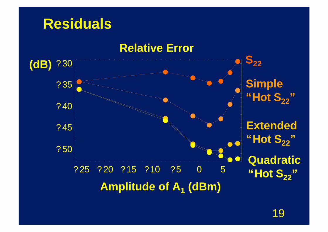
Residuals

? 25 ? 20 ? 15 ? 10 ? 5 0 5

? 50

? 45

? 40

? 35

? 30

Relative Error(dB) S22

Simple“Hot S22”

Extended“Hot S22”

Quadratic“Hot S22”

Amplitude of A1 (dBm)

20

Conclusion

• An accurate “Hot S22” exists

• It has a coefficient for the conjugate of A2.P-1

• It can accurately be measured

• It describes the relationship between A2 and B2 under large-signal excitation

21

More information

• More detailed information on this kind of measuring and modeling techniques:

http://users.skynet.be/jan.verspecht