LUND UNIVERSITY

PO Box 117221 00 Lund+46 46-222 00 00

Evaluation of Modern Irrigation Techniques with Brackish Water

Aboulila, Tarek Selim

2012

Link to publication

Citation for published version (APA):Aboulila, T. S. (2012). Evaluation of Modern Irrigation Techniques with Brackish Water. Lund University.

Total number of authors:1

General rightsUnless other specific re-use rights are stated the following general rights apply:Copyright and moral rights for the publications made accessible in the public portal are retained by the authorsand/or other copyright owners and it is a condition of accessing publications that users recognise and abide by thelegal requirements associated with these rights. • Users may download and print one copy of any publication from the public portal for the purpose of private studyor research. • You may not further distribute the material or use it for any profit-making activity or commercial gain • You may freely distribute the URL identifying the publication in the public portal

Read more about Creative commons licenses: https://creativecommons.org/licenses/Take down policyIf you believe that this document breaches copyright please contact us providing details, and we will removeaccess to the work immediately and investigate your claim.

Background and Problem Statement

1. Background and Problem Statement 1.1 Water resources and use in Egypt

Egypt has limited traditional and non-traditional water resources in relation to its population. The traditional resources include the withdrawal quota from the Nile River. Annual rainfall ranges between a maximum of about 200 mm in the northern coastal region to a minimum of nearly zero in the south, with an annual average of 51 mm (Aquastat, 2005). Also, included in the traditional resources are the shallow and renewable groundwater reservoirs in the Nile Valley, the Nile Delta, the coastal strip and the deep groundwater in the eastern desert, and the western desert and Sinai. The latter water is largely non-renewable. The non-traditional resources include reuse of agricultural drainage water and treated wastewater, as well as the desalination of seawater and brackish groundwater (Allam and Allam, 2007). According to The Ministry of Water Resources and Irrigation (MWRI, 2010), the total amount of Egyptian water resources in 2007 was 69.96 billion m3 distributed as follows: - River Nile water = 55.50 billion m3 y-1. - Groundwater in the Nile Valley and Delta = 6.10 billion m3 y-1. - Agricultural sewage water recycling = 5.70 billion m3 y-1. - Domestic and industrial sewage water recycling = 1.30 billion m3 y-1. - Rainfall and floods = 1.30 billion m3 y-1. - Sea water desalination = 0.06 billion m3 y-1.

According to the United Nations (1997), Egypt falls in the category of high water stress countries where more than 40% of its available freshwater is withdrawn. Agriculture consumes the largest amount of the Nile water and other available water resources in Egypt. According to MWRI, the total amount of water diverted for agricultural use in 2000 was 54 billion m3 y-1. This amount included water required for crop evapotranspiration (ETc), conveyance, and application losses in both the irrigation network and at the farm level (Hefny and Amer, 2005). However, the total annual municipal and industrial water use were 4.5 and 7.5 billion m3, respectively (MWRI, 2000).

Demands for water have rapidly increased during the last decade due to a growing population, increased urbanization, industrialization, food production, employment generation, higher standards of living, and agricultural policy that emphasizes expanding production in order to feed the population (Abdin and Gaafar, 2009). According to MWRI (2010), the Egyptian cultivated areas and cropped lands in 2009 were 40 and 73.5 billion m2, respectively. Its share is slightly less than 80% of the total demand for water. However, municipal water demand and water requirement for the industrial sector during 2009 were 9.0 and 8.0 billion m3, respectively. Municipal water use includes water supplies for both urban areas and rural villages. Therefore,

1

Background and Problem Statement

measures related to rationalizing agricultural water use, reducing water losses, and using alternate water resources by recycling drainage and wastewater should be implemented.

1.2 Rational agricultural water use

As seen above, water withdrawal for agriculture consumes about 80% of Egypt's water resources that mainly depends on River Nile. Currently, Egypt's water allocations are in danger as a result of the growing desire of the upstream countries to withdraw a larger quantity of the Nile water to advance their development (e.g., Ethiopia). Due to this, water availability in Egypt may decrease alarmingly and even cause famine. Therefore, strict rational agricultural water use is becoming the most effective way to cope with water scarcity and the likely problems associated with the reduction in Egypt's water allocations. Among a complete package of water saving techniques, Abdin and Gaafar (2009) presented measures related to agriculture as: - Using of modern irrigation techniques in newly reclaimed land - Change from surface to drip irrigation in the orchards and vegetable farms in old lands - Land leveling - Night irrigation - Modification of the cropping patterns - Introduction of short-age varieties - Irrigation improvement projects in the old lands

Among these measures, use of modern irrigation techniques in new reclaimed lands and implementing modern irrigation techniques in the orchards and vegetable farms in the old land instead of surface irrigation techniques are considered the most applicable and effective measure that can be conducted. Large amounts of Egypt’s water resources can be saved if modern irrigation techniques simultaneously with brackish irrigation water are used. About 21 billion m3 y-1 of water resources could be available through recycling water, changing irrigation methods, and adopting water efficient crops and cropping patterns (e.g., El-Quosy et al., 1999; Hamza and Mason, 2004).

1.3 Brackish water reuse in Egypt

In arid and semiarid countries in the Middle East, the evaporative demand is higher than precipitation. Meanwhile, there are many restrictions affecting water allocation strategies such as quantity and quality of available water, increasing water demand, etc. The use of saline water for irrigation has caught researchers’ attention due to the increasing water requirements for irrigation and the competition between human, agricultural, and industrial water use. Meanwhile, drainage water could be reused.

Reuse of drainage water has been practiced in Egypt since 1970 (Abdel-Azim and Allam, 2004). About 2.3 billion m3 of drainage water and wastewater in Upper Egypt are discharged annually to the Mediterranean Sea via return flow to the Nile River and 12 billion m3 are

2

Background and Problem Statement

discharged directly into the sea and northern lakes while 2 to 3 billion m3 are used for irrigation. Moreover, about 75% of the drainage water has a salinity of less than 4.6 dS m-1 (Abou-Zeid, 1988).

Nowadays, the policy of the country is to expand drainage water reuse to reach 8 billion m3 by 2017 (Abdin and Gaafar, 2009) while leaving a quantity not less than 8.4 billion m3 per year to be discharged to the sea to keep the salt balance for the delta region (Abdel-Azim and Allam, 2004). Currently, drainage water is used directly for irrigation if its salinity is less than 1 dS m-1 while it is mixed with Nile water if its salinity ranges from 1 to 4.6 dS m-1. The mixing ratio depends mainly on the salinity of drainage water. It is 1:1 for drainage water salinity ranging from 1 to 2.3 dS m-1 while it is 1:2 and 1:3 for salinity ranging from 2.3 to 4.6 dS m-1 (El-Gamal, 2007).

El-Salam Canal is a mixture of 2.1 billion m3 y-1 of fresh water from the River Nile and 1.9 billion m3 y-1 of drainage water. The mixing ratio is about 1:1 and the electrical conductivity, EC, of the canal water after mixing ranges from 1to 2 dS m-1 (Abou Lila et al., 2005). The canal is used to convey irrigation water to 2.6 billion m2 of reclaimed (saline) areas located to the south of El-Manzala and El-Bardawil lakes in the Eastern Delta and North Sinai. About 1.8 billion m2 of this land are located to the east of the Suez Canal and the rest is located on the western side. Up to now, about 0.2 billion m2 (clay soil with high salinity levels) and 0.8 billion m2 (coarser texture and lower salinity levels) of the land east and west of Suez Canal, respectively, have been distributed to farmers and investors.

The cultivated area in the El-Salam Canal project land is irrigated mainly by flood irrigation in clayey areas and furrow irrigation in the remaining areas. Only a small portion of the cultivated land located in the western side of Suez Canal has recently been irrigated by surface drip irrigation. The limited application of modern irrigation techniques (i.e., drip irrigation) in the El-Salam Canal project cultivated lands results from the lack of specific studies and guidelines for the suitability of these techniques with brackish irrigation water in salt-affected soils. The lack of studies in this regard hampers potential benefits of these systems in view of higher initial costs as compared to traditional irrigation methods. Moreover, more studies could show the efficiency of modern irrigation techniques in saving water and minimizing the harmful effects of using brackish irrigation water on soil salinity and groundwater salinization risk as compared to traditional irrigation methods. Therefore, providing robust instructions (i.e., guidelines) about modern irrigation techniques in the El-Salam Canal project cultivated lands will encourage the farmers to adopt modern methods and switch from their traditional methods of low efficiency (less than 50%; Postel, 2000; von Westarp et al., 2004) to modern one of high efficiency (70 to 90%; Pruitt et al., 1989; Yohannes and Tadesse, 1998; Colaizzi et al., 2006; Liao et al., 2008).

3

Background and Problem Statement

1.4 Objectives In view of the above, the problems of water scarcity, soil salinization, and groundwater

salinization risk are the main dangers threatening the agricultural environment in arid and semiarid areas (e.g., Egypt and Tunisia) nowadays that in turn affect the socioeconomic development. Using modern irrigation techniques with brackish water may be a suitable solution to cope with these problems and to prevent or reduce soil degradation under current irrigation techniques especially in salt-affected lands. Many variables need to be considered to maximize the efficiency of modern irrigation techniques with brackish irrigation water such as soil hydraulic properties, amount of irrigation water, irrigation regime, salinity of irrigation water, etc. Considering all these variables through field experiments to address the complex relation between water, soil, and crop are costly and time-consuming. However, a calibrated and validated numerical model can be used as an inexpensive, rapid, and labor saving tool for investigating irrigation efficiency under a wide range of variables and conditions. Furthermore, the model can also be used to predict soil salinity levels and groundwater contamination risks under different irrigation schedules and treatments. The objective of the present study is therefore to investigate the effect of soil type, irrigation water salinity level, irrigation regime, and geometric design aspect under different types of modern irrigation techniques on soil water and salinity distribution that in turn affect the irrigation efficiency and the surrounding environment. Also, a partial objective is to create clear guidelines for different modern irrigation techniques with brackish irrigation water in arid areas.

The thesis includes six papers that can be divided into two major categories. The first category deals with field experiments conducted in northern Tunisia to investigate soil water and salinity distribution under different treatments of drip irrigation with brackish irrigation water and to investigate the potential of groundwater contamination risk under these treatments. Further objective was to compare the mobility of different tracers under drip irrigation. Paper I compares the effect of irrigation regime on soil water and salinity distributions as well as dye infiltration under different treatments of drip irrigation (i.e., surface drip irrigation with and without plastic mulch and subsurface drip irrigation) in sandy loam soil. Furthermore, the field data are used to calibrate and validate the HYDRUS-2D/3D model. Paper II provides a study of water and solute movement beneath a single dripper with a solution containing dye and bromide in loamy sand soil. Moreover, the dye-bromide retardation factor was investigated.

In the second category of the papers, laboratory experiments were conducted to estimate soil hydraulic properties for soil samples collected from different locations within El-Salam Canal cultivated land. Then, numerical simulations with HYDRUS-2D/3D model for different irrigation techniques (surface and subsurface drip irrigation and alternate partial root-zone surface and subsurface drip irrigation) with brackish irrigation water are conducted as an attempt to create clear guidelines for these methods in arid and semiarid areas, especially, for the El-Salam Canal project region. Paper III investigates the influence of initial soil moisture content, irrigation

4

Background and Problem Statement

5

regime, and soil hydraulic properties on soil salinity levels, amount of drainage water, and amount of irrigation water that effectively can be used by the plant under surface drip irrigation (DI). Paper IV evaluates the effect of emitter depth, irrigation regime on the efficiency of subsurface drip irrigation (SDI) with brackish irrigation water in different soil types. Paper V explores the impact of emitter depth, inter-plant emitter distances, and irrigation water salinity in loamy on sand soil water and salinity distribution as well as water balance components under alternate partial root-zone subsurface drip irrigation (APRSDI). The final paper, VI, assesses the potential for execution of alternate partial root-zone surface drip irrigation (APRDI) with brackish water in salt-affected loamy sand soil taking into account the effect of inter-plant emitter distances.

Literature Review

2. Literature Review 2.1 Irrigation techniques and selection criteria Irrigation techniques are numerous and can be classified according to either their development or the way that water is applied to the soil. Flood irrigation is the oldest irrigation method used for watering crops in which a field is flooded with water that is allowed to immerse the soil to irrigate the crops. Furrow irrigation is another surface (traditional) irrigation method in which small parallel canals carry water in order to irrigate the crop that is usually grown on the ridges between the furrows. Sprinkler irrigation is one of the modern irrigation methods in which water is applied in a way similar to natural rainfall. The irrigation is developed by spraying water under pressure through small orifices or nozzles (Brouwer et al., 1988). Drip irrigation, on the other hand, is an improvement over all the aforementioned watering methods. The drip system consists of small emitters, either buried or placed on the soil surface, which discharge water at a controlled rate. Water infiltration occurs in the region directly around the emitter, which is small compared with the total soil volume of the irrigated field (Cote et al., 2003). This method varies from traditional methods or sprinkler irrigation, where water infiltrates through most or the entire soil surface (e.g., Brandt et al., 1971; Bresler, 1977).

Water use efficiency, crop yield, and soil salinity are the major factors that should be considered during the selection of irrigation method. Many studies were carried out to compare crop yield and water use efficiency under modern irrigation methods with traditional irrigation methods as well as with each other. Yang et al. (2000) compared the effect of sprinkler and flood irrigation on winter wheat yield and water use efficiency. They observed higher winter wheat yield and water use efficiency in sprinkler irrigation as compared to surface irrigation. Haijun et al. (2011) also obtained the same result in a four-year field experiment. On the other hand, Ellis et al. (1986) compared the water use efficiency for furrow, sprinkler, and surface drip irrigation (DI) when growing onion. They demonstrated higher water use efficiency for DI followed by sprinkler and furrow irrigation. Hanson et al. (1997) compared lettuce yield under furrow, surface drip, and subsurface drip irrigation (SDI) methods. They concluded that drip irrigation saved 40% of irrigation water as compared to furrow irrigation with no significant difference in crop yield. Colaizzi et al. (2006) and Liao et al. (2008) demonstrated that drip irrigation increases yields accompanied with higher field-level application efficiency as compared to other surface irrigation techniques. Sakellariou et al. (2002) compared the sugar beet yield and water use efficiency under DI and SDI systems. They indicated that SDI leads to a greater yield with significant water saving compared to DI. Conversely, Bajracharya and Sharma (2005) observed higher cucumber and tomato yield under low cost DI than in low cost SDI. Soussa (2010) compared the yield and water use efficiency under DI and SDI for growing tomato in open fields and pepper in greenhouses. The experiments were conducted in the desert regions of Egypt. She observed higher yield and water

6

Literature Review

use efficiency in the case of SDI compared to DI for the two crops. Although higher initial cost for SDI compared to sprinkle irrigation, more revenue from higher yields and reduced irrigation and cultural cost occurred when growing tomato in salt-affected areas (Hanson et al., 2006a).

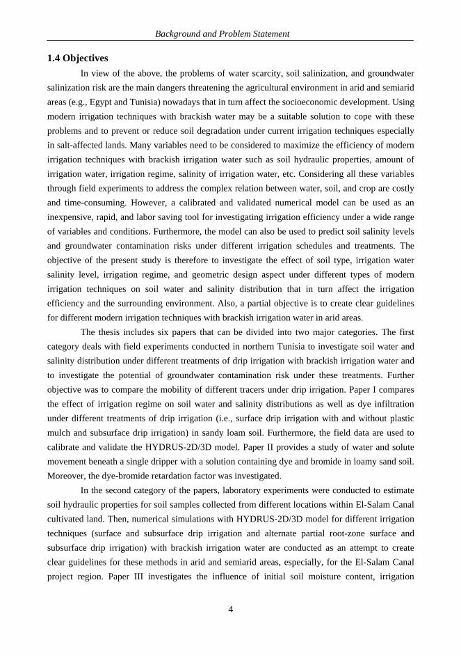
In contrast to irrigation methods that apply water at rates equal to or above full crop-water requirements (evapotranspiration), deficit irrigation is an optimizing strategy under which crops are deliberately allowed to sustain some degree of water deficit by applying water below crop evapotranspiration (e.g., Hoffman et al., 1990; Fereres and Soriano, 2007). The crop is exposed to a particular level of water deficiency either during a given period (regulated deficit irrigation) or throughout the entire growing season (classic deficit irrigation). However, it can be also practiced by exposing part of the root system to drying soil while the remaining part is irrigated normally (alternate partial root-zone irrigation; Fig. 1).

Fig. 1, Alternate partial root-zone irrigation (McCarthy et al., 2002).

The effectiveness of alternate partial root-zone irrigation (APRI) as a water-saving technique was widely investigated. Kirda et al. (2007) assessed the crop yield differences under conventional deficit irrigation (CDI), APRI, and full surface drip irrigation for different crops (e.g., tomato and pepper) in a heavy clay soil under Mediterranean climate conditions. They demonstrated that there was no significant difference in tomato yield between the APRI and full irrigation but the APRI had about 10% additional tomato yield over CDI. On the other hand, the water use efficiency was approximately the same in all irrigation methods when growing pepper. Genocoglan et al. (2006) studied the effect of green bean yield under conventional subsurface drip irrigation and alternate partial root-zone subsurface drip irrigation (APRSDI). They revealed that APRSDI saved a significant amount of irrigation water (about 50%) with same green bean yield as in SDI. Similar finding was concluded by Huang et al. (2010) when investigating potato yield under the same irrigation methods (SDI and APRSDI). The effect of APRI on soil microorganism during growing maize was studied by Wang et al. (2008). They showed that the peak numbers of

7

Literature Review

soil microorganisms were obtained in APRI compared to conventional irrigation and fixed partial root-zone irrigation. Moreover, APRI enhanced the activities of soil microorganisms needed for maize growth.

On the other hand, many studies were conducted to investigate the effect of using saline irrigation water on crop yield and water use efficiency in saline soils (e.g., Yaron et al., 1973; Bernstein and Francois, 1973; Fereres et al., 1985; Ayars et al., 1986; Cavazza, 1988; Amer and Alnagar, 1989; Saggu and Kaushal, 1991; Ayars et al., 1993; Shennan et al., 1995; Karlberg et al.,

2007; Nagaz et al., 2008). Shalhevet (1994) found that the most advantageous application method

to be used with saline water is drip irrigation. Malash et al. (2008) compared the tomato yield and water use efficiency under furrow and drip irrigation with two saline water management strategies. Saline and fresh or mixed water was applied alternatively (cyclic). The results showed that higher yield and water use efficiency occurred under drip irrigation. In addition, higher yield and water use efficiency occurred under blended strategy for both furrow and drip irrigation systems. Nagaz et al. (2008) compared the effect of drip and furrow irrigation with saline irrigation water on the yield and water use efficiency of potato in saline sandy soil in Tunisia. They concluded that higher soil salinity was maintained in the root zone with furrow as compared to drip irrigation. In addition, lower yield and water use efficiency were observed under furrow irrigation. On the other hand, Kaman et al. (2006) investigated soil salinization under APRI and compared it with conventional drip irrigation for growing tomato in a greenhouse and with conventional furrow irrigation when growing cotton in the field. They revealed that differences in salt accumulation were limited to the top 30 cm of soil profile. In addition, the soil salinity at harvest under the APRI was 35% higher than full irrigation but soil salinity levels remained below the salt tolerance threshold levels for both crops.

As seen above, drip irrigation and APRI are considered the best irrigation method and strategy that can be applied in water scarce countries characterized by arid and semiarid climate. However, more studies are still required to investigate its efficiency with brackish irrigation water and its effects on the surrounding environment, especially, in salt-affected lands. 2.2 Irrigation management Irrigation management is a key to sustain optimal crop yield with minimal amount of irrigation water (i.e., maximum water use efficiency). This also means that groundwater has to be protected. The cornerstone of irrigation management is the accurate determination of the required amount of irrigation water and the proper time for its application. Irrigation management can be conducted via three different main approaches as shown in Fig. 2.

To achieve precise irrigation management in arid and semiarid areas, there is a recognized need for knowing how water deficits and surpluses influence crop production, how to

8

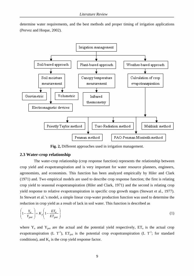
Literature Review

determine water requirements, and the best methods and proper timing of irrigation applications (Pervez and Hoque, 2002).

Fig. 2, Different approaches used in irrigation management.

2.3 Water-crop relationship The water-crop relationship (crop response function) represents the relationship between crop yield and evapotranspiration and is very important for water resource planners, engineers, agronomists, and economists. This function has been analyzed empirically by Hiler and Clark (1971) and. Two empirical models are used to describe crop response function; the first is relating crop yield to seasonal evapotranspiration (Hiler and Clark, 1971) and the second is relating crop yield response to relative evapotranspiration in specific crop growth stages (Stewart et al., 1977). In Stewart et al.’s model, a simple linear crop-water production function was used to determine the reduction in crop yield as a result of lack in soil water. This function is described as

pot

ay

pot

aETETK

YY 11 (1)

where Ya and Ypot are the actual and the potential yield respectively, ETa is the actual crop evapotranspiration (L T-1), ETpot is the potential crop evapotranspiration (L T-1; for standard conditions), and Ky is the crop yield response factor.

9

Literature Review

2.4 Soil salinity and irrigation water salinity Soil salinization is a common problem in arid and semiarid areas where the evaporation rate is higher than the precipitation rate. Naturally, soil may contain ample amount of salts due to the existence of salts in the parent rock forming soil. Seawater and shallow saline groundwater are other sources of salt in soils. A very common source of salt in irrigated land is the irrigation water itself. After irrigation, the water added to the soil is extracted by the crop or evaporates directly from the soil. The salts, however, is left behind in the soil. If not removed (leached), it accumulates in the soil and this process is called salinization (Brouwer et al., 1985). Soil salinization has two types (i.e., primary and secondary). The primary salinization is caused by the soil characteristics. However, secondary salinization is caused by irrigation.

Soil salinity is defined as the salt concentration in the water extracted from a saturated soil (called saturation extract). Rhoades et al. (1992) stated that soils with a soil water salinity less than 0.70 dS m-1 is considered to be non-saline. Irrigation water salinity is the concentration of the dissolved salts present in irrigation water and expressed in grams of salt per liter of water (g l -1), or in parts per million (ppm). The major cations of the dissolved salts are Na+, Ca2+, Mg2+, and K+ while the major anions are Cl-, HCO3

-, CO32-, SO4

2-, and NO3-. Table 1 shows the classification

and uses of water according to its salinity.

Table 1, Classification of saline waters (Rhoades, 1996)

Water class Electrical conductivity

dS/m Salt concentration

mg/l Type of water

Non-saline < 0.7 <500 Drinking and irrigation

water

Slightly saline 0.7-2 500-1500 Irrigation water

Moderately saline 2-10 1500-7000 Primary drainage water and

groundwater

Highly saline 10-25 7000-15000 Secondary drainage water

and groundwater Very highly saline

25-45 15000-35000 Very saline groundwater

Brine >45 >35000 Sea water

Due to mismanagement, improper agricultural practices, and inefficient drainage systems in Egypt, about 40% of the agricultural lands are suffering from salinization problems (Hamdy, 1999). In addition, groundwater levels are close to the soil surface most of the year. The salinization problems greatly affect the crop yield and increase the potential of groundwater contamination risks especially when using brackish irrigation water.

10

Literature Review

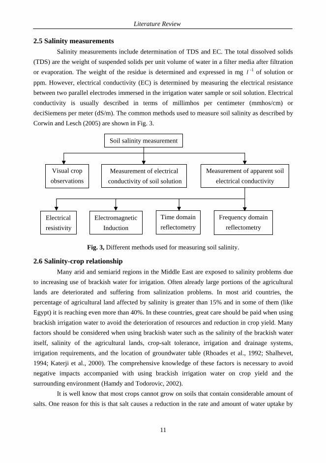
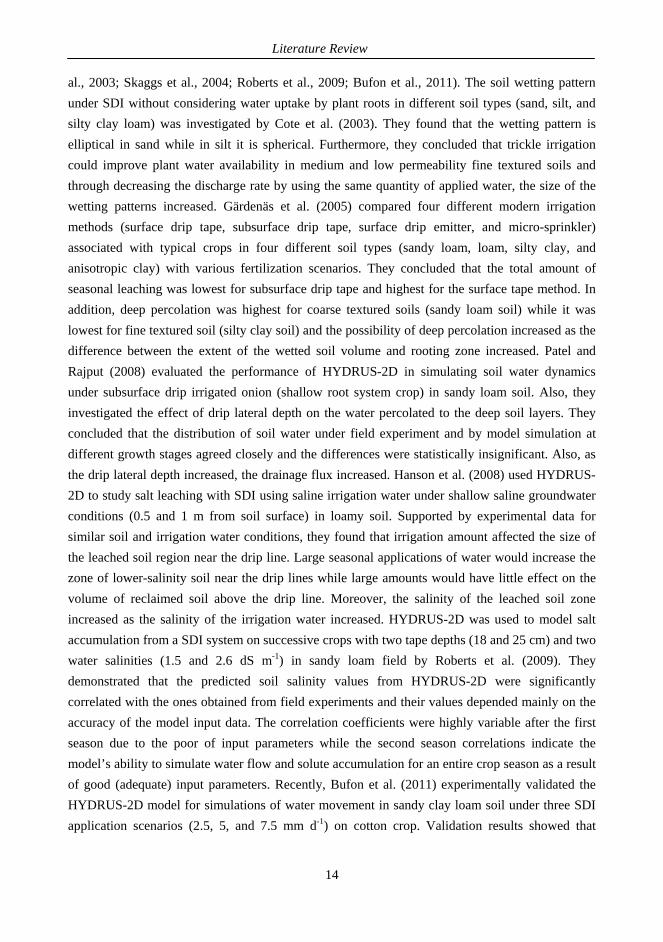
2.5 Salinity measurements Salinity measurements include determination of TDS and EC. The total dissolved solids (TDS) are the weight of suspended solids per unit volume of water in a filter media after filtration or evaporation. The weight of the residue is determined and expressed in mg -1 of solution or ppm. However, electrical conductivity (EC) is determined by measuring the electrical resistance between two parallel electrodes immersed in the irrigation water sample or soil solution. Electrical conductivity is usually described in terms of millimhos per centimeter (mmhos/cm) or deciSiemens per meter (dS/m). The common methods used to measure soil salinity as described by Corwin and Lesch (2005) are shown in Fig. 3.

l

Soil salinity measurement

Visual crop Measurement of apparent soil Measurement of electrical observations electrical conductivity conductivity of soil solution

Time domain Frequency domain Electrical Electromagnetic reflectometry reflectometry resistivity Induction

Fig. 3, Different methods used for measuring soil salinity.

2.6 Salinity-crop relationship Many arid and semiarid regions in the Middle East are exposed to salinity problems due to increasing use of brackish water for irrigation. Often already large portions of the agricultural lands are deteriorated and suffering from salinization problems. In most arid countries, the percentage of agricultural land affected by salinity is greater than 15% and in some of them (like Egypt) it is reaching even more than 40%. In these countries, great care should be paid when using brackish irrigation water to avoid the deterioration of resources and reduction in crop yield. Many factors should be considered when using brackish water such as the salinity of the brackish water itself, salinity of the agricultural lands, crop-salt tolerance, irrigation and drainage systems, irrigation requirements, and the location of groundwater table (Rhoades et al., 1992; Shalhevet, 1994; Katerji et al., 2000). The comprehensive knowledge of these factors is necessary to avoid negative impacts accompanied with using brackish irrigation water on crop yield and the surrounding environment (Hamdy and Todorovic, 2002). It is well know that most crops cannot grow on soils that contain considerable amount of salts. One reason for this is that salt causes a reduction in the rate and amount of water uptake by

11

Literature Review

the plant roots and salinity always affects yield, evapotranspiration, stomatal conductance, and leaf area (e.g., Hanson et al., 2009; Malash et al., 2008; Parida and Das, 2005). Katerji et al. (2003) studied the effects of salinity on crops yield and development. They concluded that the salinity causes reduction in crop yield by affecting the number and weight of grains, tubers, and fruits. Salinity effect also depends on other factors such as soil properties, climate conditions, irrigation practices, and water management. Salinity affects the water stress of the plant through its effect on the osmotic potential of the soil water. With increasing salinity, the osmotic potential decreases as well as the water availability for the plant, resulting in rising water stress which in turn affects stomatal conductance, leaf growth and photosynthesis (Parida and Das, 2005).

There are several approaches for predicting the decrease in crop yield due to salinity. The FAO approach assumes that crops can tolerate salinity up to a certain level without a considerable loss in yield (electrical conductivity threshold). When salinity increases beyond this threshold, crop yield decreases linearly in proportion to the increase in salinity (Allen et al., 1998).

2.7 Numerical simulation of irrigation methods

Irrigation is the major driving force for agricultural development in arid and semiarid areas. Due to the lack of available water resources, the effective use of irrigation water has become a vital issue and a key component in the production of high quality field and fruit crops. As seen above, drip irrigation is considered the best irrigation method for saving water over other irrigation methods regardless of the salinity of irrigation water.

Although some guidelines are available to apply for drip systems (e.g., Hanson et al., 1996), there is a need for better guidelines that consider differences in soil hydraulic properties (Cote et al., 2003), moreover, the influence of using brackish irrigation water in salt-affected soils should be considered. Mismanagement of irrigation systems can lead to soil salinization problems and increase the potential of groundwater salinization risk especially in the case of shallow groundwater. Therefore, improved monitoring techniques are essential to achieve the most effective management and reduce cost. Field measurements of soil moisture content and soil salinity are viable but still time and cost consuming especially for large field scale, different design aspects, various plant species, and climatic conditions. Conversely, numerical simulations can be used to overcome the aforementioned obstacles. The HYDRUS model (Simunek et al., 2008) and theMACRO model (Larsbo and Jarvis, 2003) are considered effective and accurate tools for simulating water flow and solute movement under different irrigation techniques (Phogat et al., 2011; 2010; Crevoisier et al., 2008; Patel and Rajput, 2008; Gärdenäs et al., 2005; Jarvis, 1995; Andreu et al., 1994). The HYDRUS model provides more precise estimation of water and solute dynamics under drip irrigation compared to analytical and empirical models (e.g., Kandelous and

12

Literature Review

Simunek, 2010). Analytical and empirical models require many simplifying assumptions leading to limitations in their applicability to the real field (e.g., Elmaloglou and Diamantopoulos, 2010).

Many studies have been conducted using the HYDRUS model to simulate surface drip irrigation considering different parameters (e.g., Phogat et al., 2011; Bufon et al., 2011; Ajdary et al., 2007; Skaggs et al., 2004). Assouline (2002) studied the effect of emitter discharge (0.25, 2, and 8 h-1) on different aspects of the water regime in daily drip irrigated corn on sandy loam soil. Results showed that the lowest emitter discharge led to the smallest wetted volume with the least extreme water content gradients in both horizontal and vertical direction. Moreover, it resulted in the least variable water content over a diurnal period. Skaggs et al. (2004) compared the measured and simulated water content distribution under surface drip irrigation with different irrigation levels in barren sandy loam soil at the end of irrigation and 24 h after irrigation. They found that the HYDRUS model prediction for water content distribution was in a good agreement with the measured data. Ajdary et al. (2007) studied water distribution and assessed the nitrogen leaching from onion field under drip fertigation system as well using two-year field experiment and HYDRUS model. They concluded that simulated and observed water contents and Nitrogen concentrations followed a similar trend with the determination coefficient (R2) ranging from 0.93 to 0.99 and from 0.95 to 0.99 for water content and nitrogen concentration, respectively. Skaggs et al. (2010) used HYDRUS model and field trials to investigate the effects of application rate, pulsed water application, and antecedent water content on the spreading of water from drip emitters in a barren (i.e., without crop) sandy loam soil. They concluded that the pulsing and lower application rates produced minor increase in the horizontal spreading of the wetting zone. In addition, field trials confirmed the simulation finding with no statistically significant difference. Yao et al. (2011) used HYDRUS-2D to simulate soil water dynamics in the section of jujube root zone under surface drip irrigation during a full growing season. They observed goodness of fit between the simulation and field measurements and concluded that the model performs well in simulating soil water dynamics during the entire growing season. Phogat et al. (2011) experimentally verified the HYDRUS-2D/3D for water and salinity distribution during the profile establishing stage (33 days) of almond trees under pulsed and continuous drip irrigation in salt-affected sandy soil. They demonstrated that the model closely predicted water content distribution throughout the flow domain with R2 value of 0.97 in pulsed and 0.98 in continuous drip system. In addition, the model successfully simulated the change in soil water content and soil salinity in the flow domain. After that, they studied the effect of using brackish irrigation water under pulsed and continuous drip irrigation on the leaching fraction during the establishment stage of almond. They concluded that a 75.1 and 77.6% reduction in soil salinity occurred in pulsed and continuous drip irrigation, respectively, by the end of the almond establishment stage.

l

Partial season transport of water from subsurface drip irrigation with and without plant water uptake has been successfully simulated with HYDRUS-2D (e.g., Mmolawa and Or, 2003; Cote et

13

Literature Review

al., 2003; Skaggs et al., 2004; Roberts et al., 2009; Bufon et al., 2011). The soil wetting pattern under SDI without considering water uptake by plant roots in different soil types (sand, silt, and silty clay loam) was investigated by Cote et al. (2003). They found that the wetting pattern is elliptical in sand while in silt it is spherical. Furthermore, they concluded that trickle irrigation could improve plant water availability in medium and low permeability fine textured soils and through decreasing the discharge rate by using the same quantity of applied water, the size of the wetting patterns increased. Gärdenäs et al. (2005) compared four different modern irrigation methods (surface drip tape, subsurface drip tape, surface drip emitter, and micro-sprinkler) associated with typical crops in four different soil types (sandy loam, loam, silty clay, and anisotropic clay) with various fertilization scenarios. They concluded that the total amount of seasonal leaching was lowest for subsurface drip tape and highest for the surface tape method. In addition, deep percolation was highest for coarse textured soils (sandy loam soil) while it was lowest for fine textured soil (silty clay soil) and the possibility of deep percolation increased as the difference between the extent of the wetted soil volume and rooting zone increased. Patel and Rajput (2008) evaluated the performance of HYDRUS-2D in simulating soil water dynamics under subsurface drip irrigated onion (shallow root system crop) in sandy loam soil. Also, they investigated the effect of drip lateral depth on the water percolated to the deep soil layers. They concluded that the distribution of soil water under field experiment and by model simulation at different growth stages agreed closely and the differences were statistically insignificant. Also, as the drip lateral depth increased, the drainage flux increased. Hanson et al. (2008) used HYDRUS-2D to study salt leaching with SDI using saline irrigation water under shallow saline groundwater conditions (0.5 and 1 m from soil surface) in loamy soil. Supported by experimental data for similar soil and irrigation water conditions, they found that irrigation amount affected the size of the leached soil region near the drip line. Large seasonal applications of water would increase the zone of lower-salinity soil near the drip lines while large amounts would have little effect on the volume of reclaimed soil above the drip line. Moreover, the salinity of the leached soil zone increased as the salinity of the irrigation water increased. HYDRUS-2D was used to model salt accumulation from a SDI system on successive crops with two tape depths (18 and 25 cm) and two water salinities (1.5 and 2.6 dS m-1) in sandy loam field by Roberts et al. (2009). They demonstrated that the predicted soil salinity values from HYDRUS-2D were significantly correlated with the ones obtained from field experiments and their values depended mainly on the accuracy of the model input data. The correlation coefficients were highly variable after the first season due to the poor of input parameters while the second season correlations indicate the model’s ability to simulate water flow and solute accumulation for an entire crop season as a result of good (adequate) input parameters. Recently, Bufon et al. (2011) experimentally validated the HYDRUS-2D model for simulations of water movement in sandy clay loam soil under three SDI application scenarios (2.5, 5, and 7.5 mm d-1) on cotton crop. Validation results showed that

14

Literature Review

15

HYDRUS-2D simulated volumetric soil water content within ± 3% of the measured values. Therefore, they concluded that the model can be used to evaluate irrigation strategies.

Although many numerical simulations have been conducted to investigate soil water and salinity distribution under DI and SDI, there is a lack in the simulations of alternate partial root-zone surface and subsurface drip irrigation in this regard. Most of the conducted research on APRI were field and experimental work and dealt mainly with APRI’s physiology and technical perspective while very few numerical simulation studies have been conducted for APRI (e.g., Zhou et al., 2007; 2008). Zhou et al. (2007) compared the soil water movement in a vineyard under alternate partial root-zone surface drip irrigation (APRDI) with APRI and HYDRUS-2D models. They concluded that both models performed well in simulating soil moisture dynamics under the APRDI. Zhou et al. (2008) also compared the performance of dynamic and static APRI models for simulating soil water dynamics under APRDI in the same vineyard. They demonstrated that the performance of the dynamic APRI model is better than the static APRI model.

In view of the above, there is a need for more studies related to drip irrigation and alternate partial-root zone irrigation (i.e., water conservation practices in agriculture) to investigate the effect of soil hydraulic properties, salinity of irrigation water, irrigation scheduling, and geometric design aspects on the applicability and efficiency of these methods as well as impact on the surrounding environment. Furthermore, better guidelines for these irrigation techniques are required to enhance its implementation in arid and semiarid areas and minimize the negative effects that can be accompanied with the mismanagement of these techniques.

Methodology

3. Methodology

The methodology section describes the approaches used to conduct the work in this thesis. In

section 3.1, laboratory and field experiment carried out in this thesis are described. In section 3.2,

an overview of HYDRUS-2D/3D model used to simulated different irrigation methods is

provided. The overview includes a general description of HYDRUS-2D/3D model as well as the

governing equations for water and solute transport and root water uptake. In section 3.3, a

description for the numerical simulations of different irrigation techniques included in this thesis is

addressed.

3.1 Experimental set-up 3.1.1 Laboratory experiments

The main purpose of the laboratory work was to estimate soil particle distribution, soil

bulk density, and soil water-retention characteristics for the collected soil samples from the

experimental fields in Egypt and Tunisia. Soil particle distribution and soil bulk density estimation

for soil samples collected from Egypt were carried out in the laboratory at the Department of

Lands in Agricultural Faculty, Suez Canal University, Egypt. Corresponding measurements in

Tunisia were made in the laboratory of the National Institute for Research in Rural Engineering,

Water, and Forests, Tunisia. The remaining laboratory experiments were conducted at the

Department of Water Resources Engineering laboratory, Lund University, Sweden. Both sieving

and sedimentation methods were used for particle size analysis while the pressure plate apparatus

was used to estimate soil water-retention characteristics for the collected soil samples.

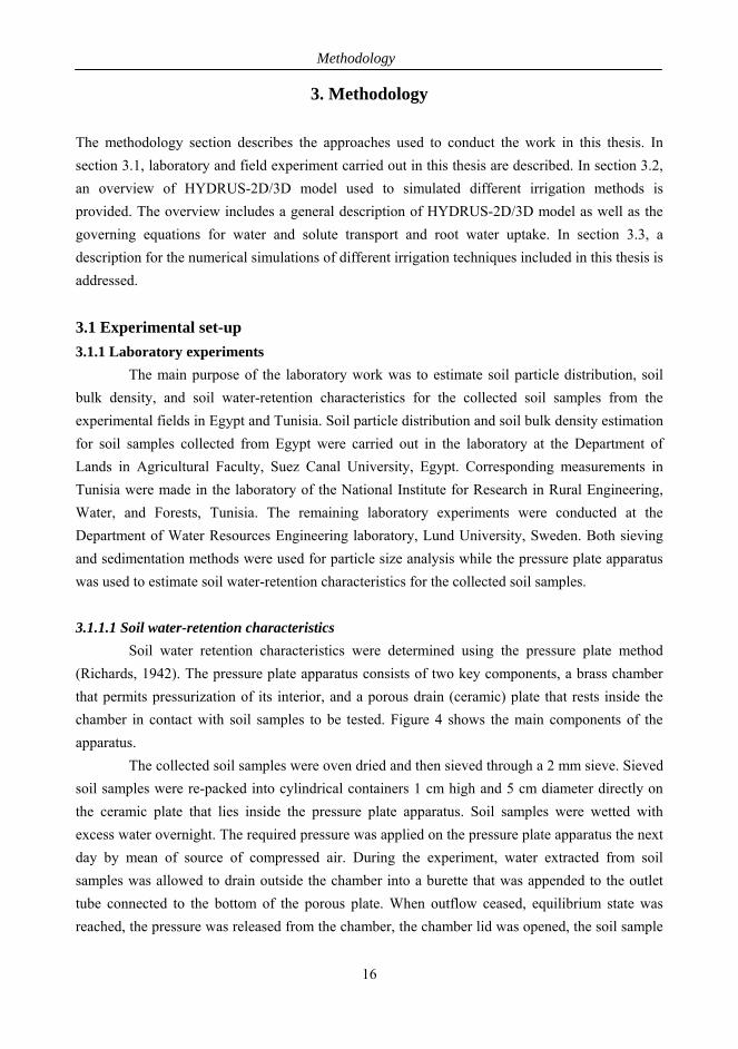
3.1.1.1 Soil water-retention characteristics Soil water retention characteristics were determined using the pressure plate method

(Richards, 1942). The pressure plate apparatus consists of two key components, a brass chamber

that permits pressurization of its interior, and a porous drain (ceramic) plate that rests inside the

chamber in contact with soil samples to be tested. Figure 4 shows the main components of the

apparatus.

The collected soil samples were oven dried and then sieved through a 2 mm sieve. Sieved

soil samples were re-packed into cylindrical containers 1 cm high and 5 cm diameter directly on

the ceramic plate that lies inside the pressure plate apparatus. Soil samples were wetted with

excess water overnight. The required pressure was applied on the pressure plate apparatus the next

day by mean of source of compressed air. During the experiment, water extracted from soil

samples was allowed to drain outside the chamber into a burette that was appended to the outlet

tube connected to the bottom of the porous plate. When outflow ceased, equilibrium state was

reached, the pressure was released from the chamber, the chamber lid was opened, the soil sample

16

Methodology

was removed from the pressure plate, weighed, and then oven dried at 105oC for 1 day for water

content determination.

Fig. 4, Pressure plate apparatus.

By using the bulk density, water content was converted to volume basis. This procedure

was repeated by increasing the pressure in the chamber; more than ten suction (pressure)

increments were used for each soil sample. A constant head permeameter (Klute and Dirksen,

1986) was used for estimating the saturated hydraulic conductivity for the tested soils. Finally, the

soil water-retention characteristics were estimated using van Genuchten-Mualem relationships

(van Genuchten, 1980).

3.1.2 Field experiments This section contains a description of the field experiments presented in the appended

papers. Two sets of field experiments were carried out. Both sets were conducted in Tunisia. In the

first set, field experiments were done to investigate water and salinity distribution as well as

contaminant transport under different treatments of drip irrigation with brackish irrigation water in

sandy loam soil. Furthermore, they were used to investigate the effect of irrigation regime on the

water and solute transport under these treatments. The results of the field experiments were also

used to validate the HYDRUS-2D/3D model. In the second set, field experiments were conducted

to investigate infiltration patterns with different tracers (dye and bromide) beneath a single dripper

in initially dry loamy sand soil. Moreover, the retardation of dye as compared to bromide was

quantified.

3.1.2.1 Drip irrigation experiments under different irrigation treatments and regimes Field experiments were carried out under different treatments of drip irrigation with a

mixture of brackish water and dye tracer. Three drip treatments namely, surface drip irrigation

17

Methodology

without and with plastic mulch (T1 and T2, respectively) and subsurface drip irrigation (T3) with a

drip tube 10 cm below soil surface were used in this work. In addition, two irrigation regimes

(daily and bi-weekly) were considered when performing each treatment.

Site description Field experiments were carried out in April 2012 (entire month) at the research station of

Souhil River, Nabeul, 70 km southeast of Tunis. The climate at Nabeul is Mediterranean semiarid

and the soil at the experimental site is classified as sandy loam. The groundwater table is located

more than 4 m below the soil surface and the initial soil moisture content changes linearly with

depth from 0.07 m3 m-3 at the soil surface to 0.10 m3 m-3 at 100 cm depth. The initial soil salinity

levels were negligible.

Experimental set-up Separated drip irrigation systems, 2.5 m apart, with a mixture of brackish water and dye

tracer were used in the field experiments. Three treatments (T1, T2, and T3) with two irrigation

regimes (daily and bi-weekly) were used during the experimental work resulting in a total of 6

experimental sets (i.e., subplots). All vegetation was carefully removed and the surface was gently

leveled without disturbing the soil structure before installing the drip system. The initial soil

moisture content was kept constant by covering the experimental plot with a plastic sheet to

prevent evaporation and rainfall infiltration. The plastic cover was only removed during irrigation

in subplots T1 and T3 and put back during the night as well as in case of rain.

The drip irrigation system used for each subplot consisted of a PVC drip tube (13 mm

internal diameter), a regulated dripper located 0.5 m from the far end of the drip tube, a small

pump, a flow control valve, a flushing valve, and a graded water tank. For each drip system, a drip

tube was connected to a small electrically driven pump that in turn was attached to the graded

water tank to generate the required pressure. Local irrigation water was mixed with Brilliant Blue

(BB) dye (2.50 g ) in order to investigate the infiltration pattern under different treatments. The

electrical conductivity of the irrigation solution after mixing was 2 dS m-1 and it was applied

through each dripper with an average discharge of 2.0 l h-1. The irrigation duration during field

experiments was 2 and 6 h per day for daily and bi-weekly irrigation strategies, respectively.

Moreover, the irrigation interval used for all treatments was 3 days leading to 12 l of dyed water

applied in each treatment (i.e., 3 irrigation events for the daily regime and one event for the bi-

weekly). Seventy-two hours after initiating the irrigation, horizontal soil sections were dug with 10

cm intervals at each subplot until the depth at which no dye traces could be seen. A scale within a

100 by 100 cm wooden frame with its origin coinciding with the dripper location was positioned

on the soil surface before taking photos. Horizontal soil sections were photographed with a digital

camera from 1.50 m height.

1l

18

Methodology

The photographs were converted to black (stained soil) and white (unstained soil) images

in Adobe Photoshop CS2 (Adobe Systems Inc.). The black and white images were then imported

in to Matlab (The Mathworks Inc.) to estimate the dye covered area. For all horizontal sections, the

WET sensor (Delta-T Devices Ltd, Cambridge, UK) was used to measure soil moisture content

and pore water electrical conductivity. Furthermore, the WET sensor readings for soil moisture

content were used to calibrate and validate the HYDRUS-2D/3D model.

3.1.2.2 Drip irrigation experiments with multiple tracers Area description

The experiments were conducted at the end of the dry season in August, 2003. The

experimental site was located at Nabeul, northern Tunisia. The soil is classified as loamy sand and

the water table is located at about 4 m depth. The field was tilled to a depth of 0.30-0.40 m. Drip

irrigation was used at this site one year before the experiments to irrigate potatoes. Three plots

(N1, N2, and N3) were chosen with an inter-plot distance of 2.5 m. The dimensions of each plot

were 2 x 2 m and the initial soil moisture content (before experiment) was 0.074 - 0.10 m3 m-3.

Experimental set-up Local irrigation water with an electrical conductivity of 3.95 dS m-1 was used for the

experiments. The irrigation water was mixed with BB dye (6 g -1) and potassium bromide (4 g -

1), resulting in a total electrical conductivity of about 10.5 dS m-1. The solute was applied through

a single dripper with a constant average flux of 2.5 l h-1. Approximately 7.5 l were discharged

from a small tank through the single dripper and a constant pressure was maintained using a small

battery-driven pump. After infiltration, the plots were covered with plastic sheet to avoid

evaporation and to protect from rain. Fifteen hours after the infiltration, horizontal soil surface

sections were dug with 5 cm intervals at each plot. A scale within a 50 by 50 cm wooden frame

with its origin coinciding with the position of the dripper was put on the soil surface before taking

photos. Horizontal soil sections were photographed with a digital camera from 1.5 m height. The

photographs were converted to black and white images in Adobe Photoshop (Adobe Systems Inc.).

Thereafter, the Matlab software was used to estimate the dye covered area. The Sigma Probe (EC1

Sigma Probe, Delta-T Devices Ltd., Cambridge, UK) was used to measure soil solution electrical

conductivity (ECw) at 5 cm intervals in a spatial grid within the 50 by 50 cm scale. The ECw

measurements were converted to relative electrical conductivity according to

l l

inp

inwrel ECEC

ECECEC

(2)

where ECin is the initial soil electrical conductivity and ECp is the electrical conductivity of the

applied pulse. The dye covered area and the Sigma Probe readings were used to estimate the

19

Methodology

bromide-dye volumetric retardation factor. The mobility of dye and bromide under drip irrigation

was also simulated using HYDRUS-2D/3D.

3.2 HYDRUS-2D/3D 3.2.1 General description of HYDRUS-2D/3D (version 1) Code

HYDRUS-2D/3D is a multi-purpose finite element model developed by J. Simunek, M.

Sejna, and M. Th. Van Genuchten in 2006. It is a Microsoft Windows based software package for

analysis of water flow and solute transport in variably saturated porous media under a wide range

of complex and irregular boundary conditions and soil heterogeneities. The program is an

extension and replacement of the variably saturated flow codes HYDRUS-2D and SWMS-3D

(Simunek et al., 2008).

The software package includes computational computer program accompanied with an

interactive graphics-based user interface that defines the overall computational domain of the

system. The model contains a project manager and both the pre-processing and the post-processing

units. The pre-processing unit facilitates discretization of the computational domain and assigning

the initial and boundary conditions. This unit contains grid generator tool for structured and

unstructured finite element meshes used for simple rectangular and complex two-dimensional

domains, respectively. It also contains both soil hydraulic parameters catalog and the Rosetta

program for predicting soil hydraulic parameters from soil textural data. The unsaturated soil

hydraulic and/or solute transport parameters can also be estimated using an indirect approach for

parameter optimization provided in HYDRUS-2D/3D. In this approach, HYDRUS-2D/3D

implement a Marquardt-Levenberg type parameter estimation technique for inverse estimation of

soil hydraulic and/or solute transport and reaction parameters based on measured transient or

steady-state flow and/or transport data (Simunek and Hopmans, 2002). The code provides three

options for weighting of inversion data; no weighting, weighting by mean ratios, and weighting by

standard deviations. When selecting no weighting option, weights should be manually assigned for

the specific data points. On the other hand, when weighting by mean ratio or by standard deviation

is chosen; the code proportionally adjusts the weights according to self-calculated means or

standard deviations of the different data sets.

The post-processing unit in the model consists of graphical presentations for the

computation outputs. These presentations started from its simplest shape (spatial and temporal x-y

graphics) reached to its complex forms (contour maps, isolines, and spectral maps). For further

details about HYDRUS-2D/3D model and its applications, see Radcliffe and Simunek (2010).

20

Methodology

3.2.2 Governing equations 3.2.2.1 Flow equation

HYDRUS-2D/3D uses the modified form of Richards’ equation (Richards, 1931) to

describe water flow in isotropic variably saturated porous media as

AKijjx

h

+ )] - S (3)

t

= ix

[K ( AKiz

where θ is volumetric soil water content (L3 L−3), h is the soil water potential expressed by

pressure head (L), t is the time (T), S is a sink term (L3 L-3 T−1), xi (i = 1,2) are the spatial

coordinates (L), are components of a dimensionless anisotropy tensor AijK AK (which reduces to

the unit matrix when the medium is isotropic, and K is the unsaturated hydraulic conductivity

function (L T-1) given by

K(h, x, y, z) = Ks (x, y, z) Kr (h, x, y, z) (4)

where Kr and Ks are the relative and saturated hydraulic conductivity (L T-1), respectively.

When applying the modified form of Richards’ equation to planar flow in a vertical cross-

section, x1 = x (horizontal coordinate) and x2 = z (the vertical coordinate and taken positive

upward) and the equation will be in the form

t

= x

x

h K(h) +

z

K(h) z

h K(h) - S (5)

Numerical solution of the flow equation requires knowledge of soil water characteristics

and soil saturated hydraulic conductivity. One of the analytical models for estimating soil

hydraulic properties used in HYDRUS-2D/3D is the van Genuchten-Mualem constitutive

relationships:

+ mnrs

h

1

h < 0 r

h 0 s

h = (6)

K(h) = Ks (7) leS 2)1(1 /1 mm

eS

where h is the soil water retention (L3 L-3), s , r are the saturated and residual water content,

respectively (L3 L-3), α is related to the inverse of a characteristic pore radius (L-1), is shape

parameter, n is a pore-size distribution index, m = 1-1/n, and Se is the effective saturation given by

l

21

Methodology

rs

reS

(8)

3.2.2.2 Solute transport equation Physical transport, chemical interaction, and biological processes govern fluxes of solute

in soil (Cote et al., 2003). HYDRUS-2D/3D simulates solute transport based on the advection-

dispersion equation considering advective-dispersive transport in the liquid phase and diffusion in

the gaseous phase. The transport equations also guarantee the simulation of linear equilibrium

reactions between the liquid and gaseous phases, non-linear non-equilibrium reactions between the

solid and liquid phases, and two first-order degradation reactions. Nevertheless, physical non-

equilibrium solute transport can be simulated by using dual-porosity option that divides the liquid

phase into mobile and immobile regions. In addition, simulation of viruses, colloids, and bacteria

transport can be conducted based on attachment/detachment theory.

By ignoring chemical interactions and biological processes, the governing advection-

dispersion equation for the transport of single non-reactive ion in homogeneous medium is

described as

tc

= ix

x

c

iijD -

ix

c

iq

- Sc (9)

where c is the concentration of the solute in the soil water (liquid phase; M L-3), the subscripts i and j denote rather x or z, qi is the components of the volumetric flux density, and Dij is the

dispersion coefficient (L2 T-1), Sc is the plant solute uptake. The first term on the right hand side

refers to the solute flux due to dispersion and the second term denotes to the solute flux due to

convection with flowing water.

3.2.3 Root water uptake The sink term, S, in Eqn. (3) assigns the actual volume of water removed per unit time

from a unit volume of soil as a result of plant consumption and is defined as

S(h) = α(h) Sm (10)

where α(h) is the plant water stress response function and Sm is the normalized (maximum

possible) root water uptake [T-1]. The Sm is a function of root characteristics and the

meteorological conditions such as evaporative demand. When the normalized water uptake rate is

distributed evenly over a two-dimensional rectangular domain, Sm becomes

Sm = zx

ps

LLTL

(11)

22

Methodology

where Tp is the potential transpiration rate (L T-1), Ls is the width of the soil surface (L), Lx is the

width of the root zone (L), and Lz is the depth of the root zone (L). Vogel (1978) presented a

generalization of Eqn. (11) by introducing a non-uniform distribution of the normalized water

uptake rate over a root zone with an arbitrary shape as

Sm = b(x, y, z) LsTp (12)

where b(x, y, z) is a normalized root water uptake distribution (L-2 or L-3) and is a function of the

spatial location within the multi-dimensional root domain. If b(x, y, z) is integrated over the region

occupied by the root zone ( R ), it will equal to 1. b(x, y, z) is obtained from

b(x, y, z) =

R

dzyx

zyx

),,(

),,(

(13)

where ),,( zyx denotes the dimensionless spatial root distribution function. The two- and three-

dimensional root distribution function as described by Vrugt et al. (2001) and applied in HYDRUS

code are

β(x, y) =

zzZpxx

Xp

mm

m

z

m

x

eZz

Xx

**

11 (14)

β(x, y, z) =

zzZpyy

Yp

xxXp

mmm

m

z

m

y

m

x

eZz

Yy

Xx

***

111 (15)

where Xm, Ym, and Zm are the maximum rooting lengths in the x-, y-, and z- directions (L),

respectively; x, y, and z are distances from the origin of the plant in the x-, y-, and z- directions

(L), respectively; x* (L) , y* (L), and z* (L) indicated as length of maximum root intensity in the

x-, y-, and z- directions, respectively; and px (-), py (-) , pz (-) are empirical parameters. These

parameters were used to provide zero root water uptake at x ≥ Xm, y ≥ Ym, and z ≥ Zm and to allow

for root water uptake otherwise. Empirical parameters px (-), py (-) , and pz are assumed equal to

unity for x > x*, y > y*, and z > z*, respectively. It is worth noting that z coordinate for the root

distribution starts at the highest located node of the entire flow domain while x and y coordinates

coincide with x and y coordinates according to the geometry of flow domain.

By using the Vrugt et al. (2001) description, the normalized root water uptake in two and

three dimensions takes the form

Sm =

m mX Z

pm

dxdzzyx

TzyxX

0 0

),,(

),,(

(16)

23

Methodology

Sm =

m m mX Y Z

pmm

dxdydzzyx

TzyxYX

0 0 0

),,(

),,(

(17)

From Eqn. (10) it is clear that the normalized root water uptake is equal to the actual root

water uptake during periods of no water stress, at optimal conditions, when α(h) =1. Under non-

optimal conditions; high evaporative demand of the atmosphere and/or conditions of water and/or

salinity stress, the actual root water uptake is less than the normalized root water uptake.

HYDRUS-2D/3D allows considering the effect of water stress or/and salinity stress when

calculating the actual root water uptake.

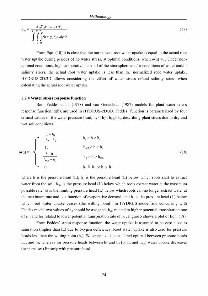
3.2.4 Water stress response function Both Feddes et al. (1978) and van Genuchten (1987) models for plant water stress

response function, α(h), are used in HYDRUS-2D/3D. Feddes’ function is parameterized by four

critical values of the water pressure head, h3 < h2< hopt< ho describing plant stress due to dry and

wet soil conditions

32

3

hhhh

h2 > h > h3

1,

oopt

ohh

hh

0

hopt > h > h2 (18) α(h) =

ho > h > hopt

ho h3 or h h

where h is the pressure head (L), ho is the pressure head (L) below which roots start to extract

water from the soil, hopt is the pressure head (L) below which roots extract water at the maximum

possible rate, h2 is the limiting pressure head (L) below which roots can no longer extract water at

the maximum rate and is a function of evaporative demand, and h3 is the pressure head (L) below

which root water uptake ceases (the wilting point). In HYDRUS model and concurring with

Feddes model two values of h2 should be assigned; h2H related to higher potential transpiration rate

of r2H and h2L related to lower potential transpiration rate of r2L. Figure 5 shows a plot of Eqn. (18).

From Feddes’ stress response function, the water uptake is assumed to be zero close to

saturation (higher than ho) due to oxygen deficiency. Root water uptake is also zero for pressure

heads less than the wilting point (h3). Water uptake is considered optimal between pressure heads

hopt and h2, whereas for pressure heads between h2 and h3 (or ho and hopt) water uptake decreases

(or increases) linearly with pressure head.

24

Methodology

hopt

Fig. 5, Feddes et al. (1978) water stress response function.

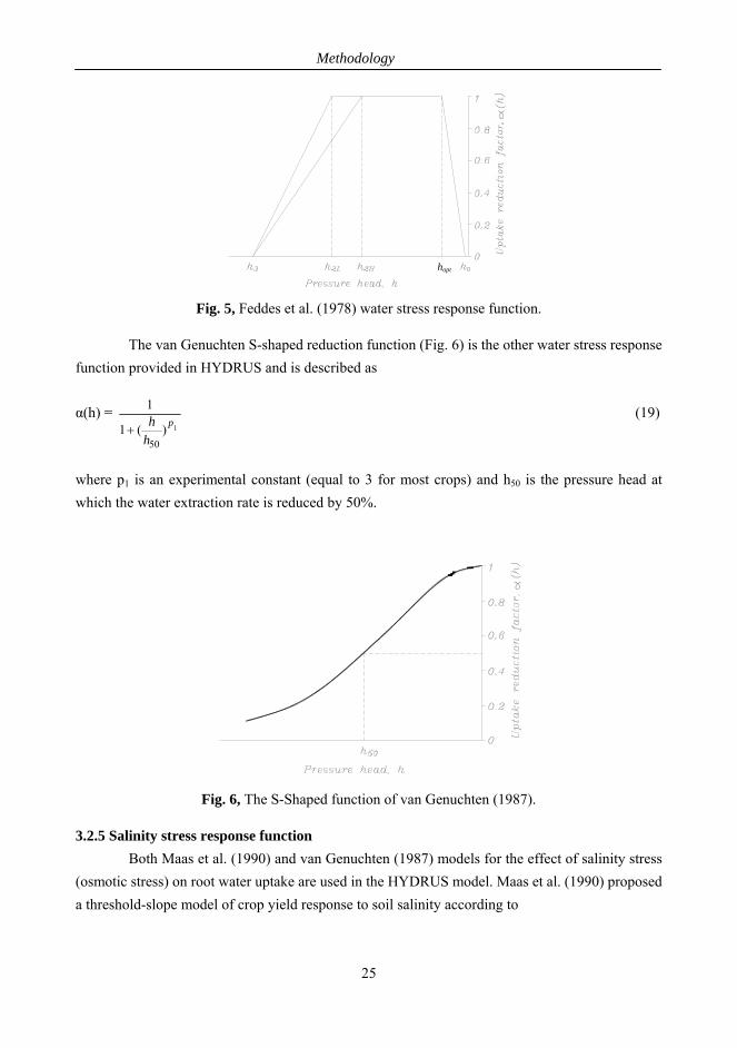
The van Genuchten S-shaped reduction function (Fig. 6) is the other water stress response

function provided in HYDRUS and is described as

α(h) = 1)(1

1

50

p

hh

(19)

where p1 is an experimental constant (equal to 3 for most crops) and h50 is the pressure head at

which the water extraction rate is reduced by 50%.

Fig. 6, The S-Shaped function of van Genuchten (1987).

3.2.5 Salinity stress response function Both Maas et al. (1990) and van Genuchten (1987) models for the effect of salinity stress

(osmotic stress) on root water uptake are used in the HYDRUS model. Maas et al. (1990) proposed

a threshold-slope model of crop yield response to soil salinity according to

25

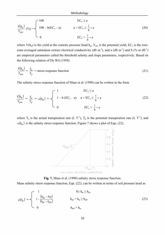
Methodology

100 ECe ≤ a

potYhY (%) = 100 – b(ECe – a) a < ECe ≤ a

b

1 (20)

0 ECe > ab

1

where Y(hφ) is the yield at the osmotic pressure head hφ, Ypot is the potential yield, ECe is the root-

zone-averaged saturation extract electrical conductivity (dS m-1), and a (dS m-1) and b (% m dS-1)

are empirical parameters called the threshold salinity and slope parameters, respectively. Based on

the following relation of De Wit (1958)

potYhY =

p

aTT

= stress response function (21)

The salinity stress response function of Maas et al. (1990) can be written in the form

1 ECe ≤ a

1 – b (ECe – a) a < ECe ≤ ab

1 (22)

0 ECe >

potYhY =

p

aTT = h =

ab

1

where Ta is the actual transpiration rate (L T-1), Tp is the potential transpiration rate (L T-1), and

h is the salinity stress response function. Figure 7 shows a plot of Eqn. (22).

Fig. 7, Maas et al. (1990) salinity stress response function.

Maas salinity stress response function, Eqn. (22), can be written in terms of soil pressure head as

1 0≥ hφ ≥ hφt

h = 0

1

hhhh

t

t

hφt > hφ ≥ hφ0 (23)

0 hφ0 > hφ

26

Methodology

where hφ is the osmotic head (L), hφt is the threshold value of hφ above which h equal to 1,

and hφ0 is the threshold value of hφ below which h equals 0.

The van Genuchten S-shaped model is the other salinity stress response function used in

HYDRUS-2D/3D. Similar to van Genuchten water stress response function, a salinity stress

response function is introduced as

2

501

1p

hh

h

(24)

where hφ50 represents the osmotic head at which the water extraction rate is reduced by 50% and p2

is an experimental constant.

3.2.6 Combined water and salinity stress response function

The combined effect of water and salinity stress on root water uptake in HYDRUS-

2D/3D is considered using additive or multiplicative models. In the additive model, salinity stress

is added to water stress by replacing the pressure head in the soil, h, by the sum of water and

osmotic pressure heads, h and hφ. However, in the multiplicative model, the root water uptake

reduction due to water stress and salinity stress are multiplied ( hhhh , ). When the

multiplicative model is used for salinity stress, both threshold model (Maas, 1990) or the S-shaped

model (van Genuchten, 1987) can be used. The S-shaped model for combining the effect of water

and salinity stress in multiplicative basis is defined as

α (h, hφ) = 1)(1

1

50

p

hh

2)(1

1

50

phh

(25)

where p1 and p2 are experimental constants, h50 represents the pressure head at which the water

extraction rate is reduced by 50% during conditions of negligible osmotic stress, and hφ50

represents the osmotic head at which the water extraction rate is reduced by 50% during conditions

of negligible water stress. However, the threshold model simulates the osmotic stress with two

variables: the threshold, value of the minimum osmotic head above which root water uptake occurs

without a reduction; and the slope, the slope of the line determining the fractional root water

uptake decline per unit increase in salinity below the threshold. It is pertinent to mention that

HYDRUS-2D/3D model contains a list for crop-specific parameters for water uptake and solute

stress.

27

Methodology

3.3 Numerical simulation In this section, numerical simulations for field experiments conducted in Tunisia were

carried out using HYDRUS-2D/3D. Furthermore, an numerical assessment for various modern

irrigation techniques (surface drip irrigation, subsurface drip irrigation, alternate partial root-zone

surface drip irrigation, and alternate partial root-zone subsurface drip irrigation) in different soil

types of the El-Salam Canal cultivated land with different design aspects and different irrigation

water salinity were performed. The aim of the numerical simulations of Tunisian experiments was

to validate the HYDRUS-2D/3D model and to extrapolate the ability of HYDRUS model for

reducing the dependency on experimental research. However, the aim of the numerical simulations

for the various modern irrigation techniques in different soil types of the El-Salam Canal

cultivated land was to 1) investigate the effect of the design aspects and irrigation water salinity

levels on soil water and salinity distribution, 2) study the influence of soil hydraulic properties on

wetting patterns and salinity distribution, 3) study the effect of brackish irrigation water on

surrounding environment, specifically, the groundwater contamination risk, and 4) provide

insights to develop clear guidelines for proper design and management of modern irrigation

techniques. These insights are essential to confirm and demonstrate to local farmers the efficiency

of modern irrigation techniques in saving water and minimizing harmful effects of using brackish

irrigation water as compared to conventional irrigation.

3.3.1 Numerical simulation of Tunisian experiments 3.3.1.1 Simulation of drip irrigation under different irrigation treatments and regimes

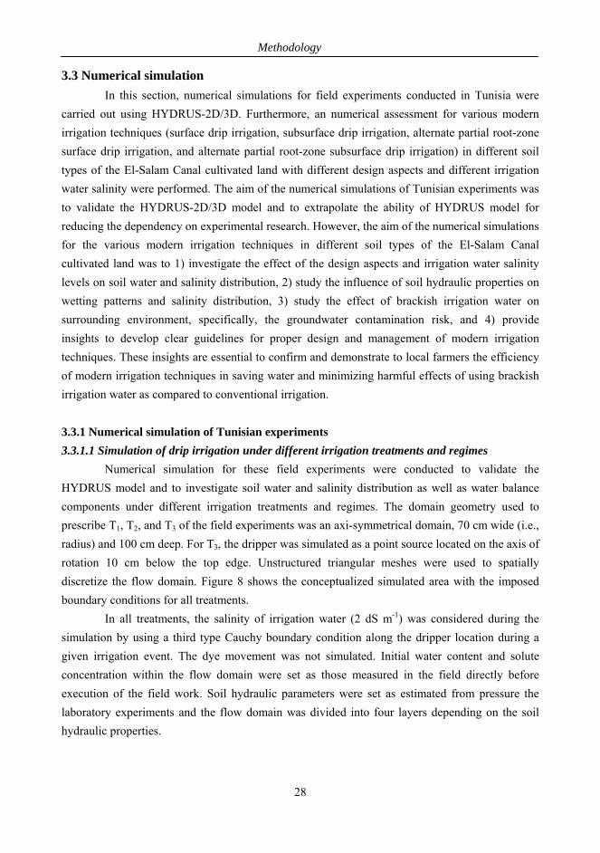
Numerical simulation for these field experiments were conducted to validate the

HYDRUS model and to investigate soil water and salinity distribution as well as water balance

components under different irrigation treatments and regimes. The domain geometry used to

prescribe T1, T2, and T3 of the field experiments was an axi-symmetrical domain, 70 cm wide (i.e.,

radius) and 100 cm deep. For T3, the dripper was simulated as a point source located on the axis of

rotation 10 cm below the top edge. Unstructured triangular meshes were used to spatially

discretize the flow domain. Figure 8 shows the conceptualized simulated area with the imposed

boundary conditions for all treatments.

In all treatments, the salinity of irrigation water (2 dS m-1) was considered during the

simulation by using a third type Cauchy boundary condition along the dripper location during a

given irrigation event. The dye movement was not simulated. Initial water content and solute

concentration within the flow domain were set as those measured in the field directly before

execution of the field work. Soil hydraulic parameters were set as estimated from pressure the

laboratory experiments and the flow domain was divided into four layers depending on the soil

hydraulic properties.

28

Methodology

Fig. 8, Conceptual diagram of simulated area with different treatments.

Solute parameters required during simulation were longitudinal and lateral dispersivities

(εL, εT; respectively). εL was set equal to one-tenth of the profile depth (e.g., Anderson, 1984; Cote

et al., 2001) while εT was set equal to 0.1 εL. Molecular diffusion and the adsorption isotherm

coefficient were neglected during simulation. The convection dispersion equation for non-reactive

solutes was used during simulation and the simulations were conducted for a 72 h period.

Twenty eight observation points were selected in the HYDRUS model situated at seven

depths between the soil surface and a depth of 60 cm (at intervals of 10 cm) and at four horizontal

distances 10 cm apart (starting from the left boundary) to observe the water content at the end of

simulation period. These values were used during model calibration and validation.

Surface drip irrigation treatment with plastic mulch (T2) accompanied with daily

irrigation was used during model calibration. As soil hydraulic properties ( ,,,, lsr and n) of

different soil layers were pre-determined via standard laboratory methods, model calibration was

conducted for soil saturated hydraulic conductivity (Ks). After calibration, the model was

validated to examine its predictability by comparing the predicted and observed water content data

for the remaining irrigation treatments and regimes.

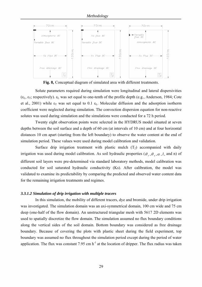
3.3.1.2 Simulation of drip irrigation with multiple tracers

In this simulation, the mobility of different tracers, dye and bromide, under drip irrigation

was investigated. The simulation domain was an axi-symmetrical domain, 100 cm wide and 75 cm

deep (one-half of the flow domain). An unstructured triangular mesh with 5617 2D elements was

used to spatially discretize the flow domain. The simulation assumed no flux boundary conditions

along the vertical sides of the soil domain. Bottom boundary was considered as free drainage

boundary. Because of covering the plots with plastic sheet during the field experiment, top

boundary was assumed no flux throughout the simulation period except during the period of water

application. The flux was constant 7.95 cm h-1 at the location of dripper. The flux radius was taken

29

Methodology

equal to 10 cm as neither ponding nor surface runoff was assumed to occur. Figure 9 shows the

conceptualized simulated area and the imposed boundary conditions.

The εL was approximated to one-tenth of the profile depth and εT was set equal to 0.1 εL.

Dye adsorption isotherm coefficient was set equal to 0.10 cm3 g-1 (Öhrström et al., 2004), and

molecular diffusion coefficients in free water were 0.0738 and 0.0036 cm2 h-1 for bromide and dye

respectively. The initial θ distribution within the flow domain was chosen related to the field

measurements. The simulations were conducted for an 18-h period.

Fig. 9, Conceptual diagram of simulated area.

3.3.2 Numerical simulation for various modern irrigation techniques within El-Salam Canal cultivated region

Area description In this part of the thesis, I focused on the main soil types of El-Salam Canal cultivated

land located in North Sinai. The soil salinity of the study area ranges from 1.70 to 2.50 dS m-1 as

recorded by soil salinity measurements conducted in previous field experiments by the end of 2005

(Abou Lila et al., 2005).

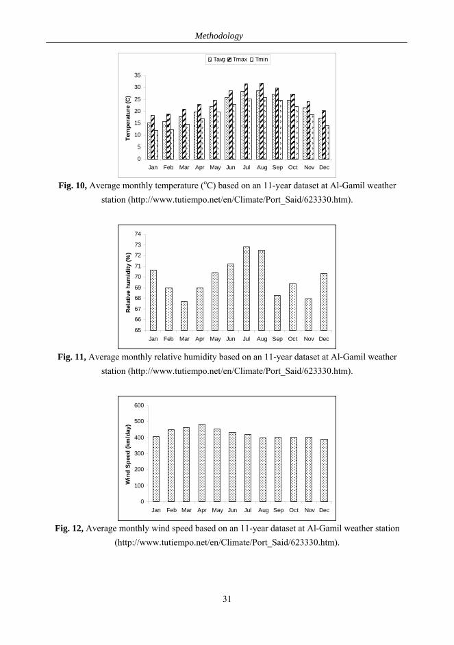
The El-Salam Canal cultivated land region is characterized by high summer ambient

temperatures, high wind speed, and low annual rainfall. The annual rainfall is approximately 150

mm with high annual potential evapotranspiration. The meteorological data of the study area were

collected from Al-Gamil weather station that is the nearest station to the study area. Figures 10-12

show the average monthly meteorological data (maximum temperature, average temperature,

minimum temperature, relative humidity, and wind speed) from 2000 to 2010 used to calculate the

crop evapotranspiration within the study area.

30

Methodology

0

5

10

15

20

25

30

35

Jan Feb Mar Apr May Jun Jul Aug Sep Oct Nov Dec

Tem

pera

ture

(C)

Tavg Tmax Tmin

Fig. 10, Average monthly temperature (oC) based on an 11-year dataset at Al-Gamil weather

station (http://www.tutiempo.net/en/Climate/Port_Said/623330.htm).

65

66

67

68

69

70

71

72

73

74

Jan Feb Mar Apr May Jun Jul Aug Sep Oct Nov Dec

Rela

tive

hum

idity

(%)

Fig. 11, Average monthly relative humidity based on an 11-year dataset at Al-Gamil weather

station (http://www.tutiempo.net/en/Climate/Port_Said/623330.htm).

0

100

200

300

400

500

600

Jan Feb Mar Apr May Jun Jul Aug Sep Oct Nov Dec

Win

d S

peed

(km

/day

)

Fig. 12, Average monthly wind speed based on an 11-year dataset at Al-Gamil weather station

(http://www.tutiempo.net/en/Climate/Port_Said/623330.htm).

31

Methodology

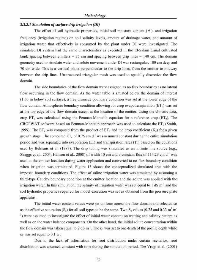
3.3.2.1 Simulation of surface drip irrigation (DI) The effect of soil hydraulic properties, initial soil moisture content ( i ), and irrigation

frequency (irrigation regime) on soil salinity levels, amount of drainage water, and amount of

irrigation water that effectively is consumed by the plant under DI were investigated. The

simulated DI system had the same characteristics as executed in the El-Salam Canal cultivated

land; spacing between emitters = 35 cm and spacing between drip lines = 140 cm. The domain

geometry used to simulate water and solute movement under DI was rectangular, 100 cm deep and

70 cm wide. This is a vertical plane perpendicular to the drip lines, from the emitter to midway

between the drip lines. Unstructured triangular mesh was used to spatially discretize the flow

domain.

The side boundaries of the flow domain were assigned as no flux boundaries as no lateral

flow occurring in the flow domain. As the water table is situated below the domain of interest

(1.50 m below soil surface), a free drainage boundary condition was set at the lower edge of the

flow domain. Atmospheric boundary condition allowing for crop evapotranspiration (ETc) was set

at the top edge of the flow domain except at the location of the emitter. Using the climatic data,

crop ETc was calculated using the Penman-Monteith equation for a reference crop (ET0). The

CROPWAT software based on Penman-Monteith approach was used to calculate the ET0 (Smith,

1999). The ETc was computed from the product of ET0 and the crop coefficient (Kc) for a given

growth stage. The computed ETc of 0.75 cm d-1 was assumed constant during the entire simulation

period and was separated into evaporation (Ep) and transpiration rates (Tp) based on the equations

used by Belmans et al. (1983). The drip tubing was simulated as an infinite line source (e.g.,

Skaggs et al., 2004; Hanson et al., 2008) of width 10 cm and a constant flux of 114.29 cm d-1 was

used at the emitter location during water application and converted to no flux boundary condition

when irrigation was terminated. Figure 13 shows the conceptualized simulated area with the

imposed boundary conditions. The effect of saline irrigation water was simulated by assuming a

third-type Cauchy boundary condition at the emitter location and the solute was applied with the

irrigation water. In this simulation, the salinity of irrigation water was set equal to 1 dS m-1 and the

soil hydraulic properties required for model execution was set as obtained from the pressure plate

apparatus.

The initial water content values were set uniform across the flow domain and selected so

as the effective saturation (Se) for all soil types to be the same. Two Se values (0.25 and 0.33 m3 m-

3) were assumed to investigate the effect of initial water content on wetting and salinity pattern as

well as on the water balance components. On the other hand, the initial solute concentration within

the flow domain was taken equal to 2 dS m-1. The εL was set to one-tenth of the profile depth while

εT was set equal to 0.1 εL.

Due to the lack of information for root distribution under certain scenarios, root

distribution was assumed constant with time during the simulation period. The Vrugt et al. (2001)

32

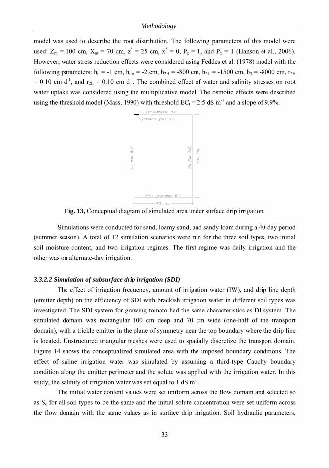
Methodology

model was used to describe the root distribution. The following parameters of this model were

used: Zm = 100 cm, Xm = 70 cm, z* = 25 cm, x* = 0, Pz = 1, and Px = 1 (Hanson et al., 2006).

However, water stress reduction effects were considered using Feddes et al. (1978) model with the

following parameters: ho = -1 cm, hopt = -2 cm, h2H = -800 cm, h2L = -1500 cm, h3 = -8000 cm, r2H

= 0.10 cm d-1, and r2L = 0.10 cm d-1. The combined effect of water and salinity stresses on root

water uptake was considered using the multiplicative model. The osmotic effects were described

using the threshold model (Mass, 1990) with threshold ECt = 2.5 dS m-1 and a slope of 9.9%.

Fig. 13, Conceptual diagram of simulated area under surface drip irrigation.

Simulations were conducted for sand, loamy sand, and sandy loam during a 40-day period

(summer season). A total of 12 simulation scenarios were run for the three soil types, two initial

soil moisture content, and two irrigation regimes. The first regime was daily irrigation and the

other was on alternate-day irrigation.

3.3.2.2 Simulation of subsurface drip irrigation (SDI)

The effect of irrigation frequency, amount of irrigation water (IW), and drip line depth

(emitter depth) on the efficiency of SDI with brackish irrigation water in different soil types was

investigated. The SDI system for growing tomato had the same characteristics as DI system. The

simulated domain was rectangular 100 cm deep and 70 cm wide (one-half of the transport

domain), with a trickle emitter in the plane of symmetry near the top boundary where the drip line

is located. Unstructured triangular meshes were used to spatially discretize the transport domain.

Figure 14 shows the conceptualized simulated area with the imposed boundary conditions. The

effect of saline irrigation water was simulated by assuming a third-type Cauchy boundary

condition along the emitter perimeter and the solute was applied with the irrigation water. In this

study, the salinity of irrigation water was set equal to 1 dS m-1.

The initial water content values were set uniform across the flow domain and selected so

as Se for all soil types to be the same and the initial solute concentration were set uniform across

the flow domain with the same values as in surface drip irrigation. Soil hydraulic parameters,

33

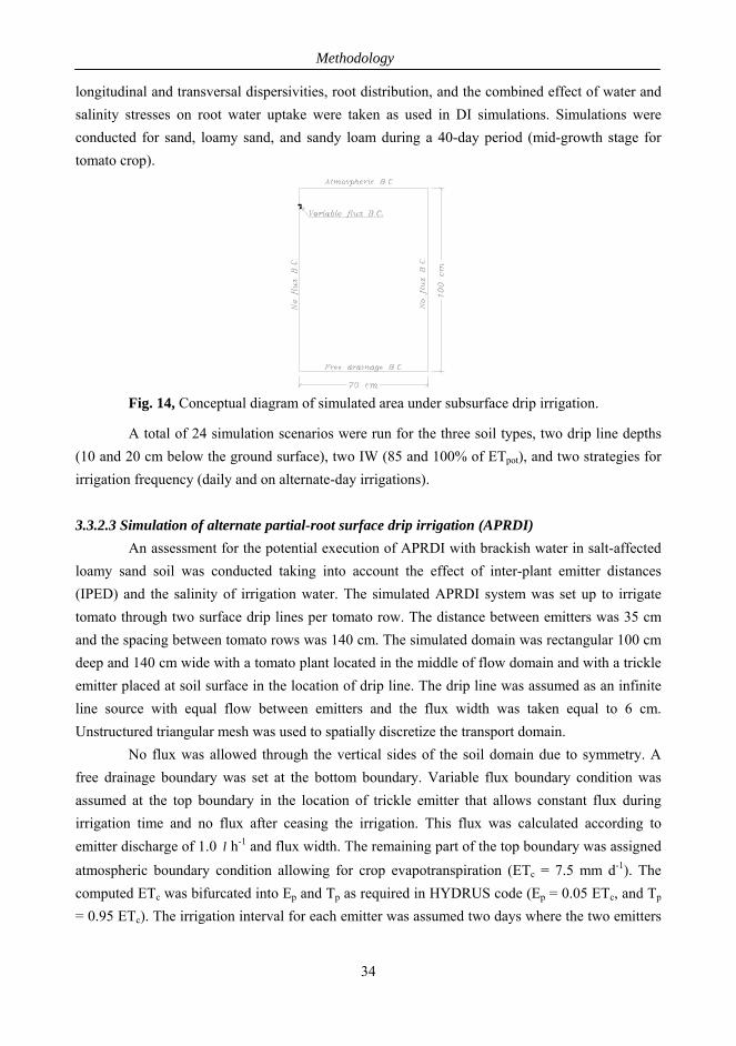
Methodology

longitudinal and transversal dispersivities, root distribution, and the combined effect of water and

salinity stresses on root water uptake were taken as used in DI simulations. Simulations were

conducted for sand, loamy sand, and sandy loam during a 40-day period (mid-growth stage for

tomato crop).

Fig. 14, Conceptual diagram of simulated area under subsurface drip irrigation.

A total of 24 simulation scenarios were run for the three soil types, two drip line depths

(10 and 20 cm below the ground surface), two IW (85 and 100% of ETpot), and two strategies for

irrigation frequency (daily and on alternate-day irrigations).

3.3.2.3 Simulation of alternate partial-root surface drip irrigation (APRDI) An assessment for the potential execution of APRDI with brackish water in salt-affected

loamy sand soil was conducted taking into account the effect of inter-plant emitter distances

(IPED) and the salinity of irrigation water. The simulated APRDI system was set up to irrigate

tomato through two surface drip lines per tomato row. The distance between emitters was 35 cm

and the spacing between tomato rows was 140 cm. The simulated domain was rectangular 100 cm

deep and 140 cm wide with a tomato plant located in the middle of flow domain and with a trickle

emitter placed at soil surface in the location of drip line. The drip line was assumed as an infinite

line source with equal flow between emitters and the flux width was taken equal to 6 cm.

Unstructured triangular mesh was used to spatially discretize the transport domain.

No flux was allowed through the vertical sides of the soil domain due to symmetry. A

free drainage boundary was set at the bottom boundary. Variable flux boundary condition was

assumed at the top boundary in the location of trickle emitter that allows constant flux during

irrigation time and no flux after ceasing the irrigation. This flux was calculated according to

emitter discharge of 1.0 l h-1 and flux width. The remaining part of the top boundary was assigned

atmospheric boundary condition allowing for crop evapotranspiration (ETc = 7.5 mm d-1). The

computed ETc was bifurcated into Ep and Tp as required in HYDRUS code (Ep = 0.05 ETc, and Tp

= 0.95 ETc). The irrigation interval for each emitter was assumed two days where the two emitters

34

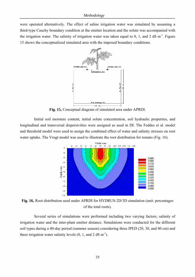
Methodology

were operated alternatively. The effect of saline irrigation water was simulated by assuming a

third-type Cauchy boundary condition at the emitter location and the solute was accompanied with

the irrigation water. The salinity of irrigation water was taken equal to 0, 1, and 2 dS m-1. Figure

15 shows the conceptualized simulated area with the imposed boundary conditions.

Fig. 15, Conceptual diagram of simulated area under APRDI.

Initial soil moisture content, initial solute concentration, soil hydraulic properties, and

longitudinal and transversal dispersivities were assigned as used in DI. The Feddes et al. model

and threshold model were used to assign the combined effect of water and salinity stresses on root

water uptake. The Vrugt model was used to illustrate the root distribution for tomato (Fig. 16).

Fig. 16, Root distribution used under APRDI for HYDRUS-2D/3D simulation (unit: percentages

of the total roots).

Several series of simulations were performed including two varying factors; salinity of

irrigation water and the inter-plant emitter distance. Simulations were conducted for the different

soil types during a 40-day period (summer season) considering three IPED (20, 30, and 40 cm) and

three irrigation water salinity levels (0, 1, and 2 dS m-1).

35

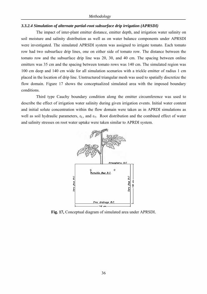
Methodology

36

3.3.2.4 Simulation of alternate partial-root subsurface drip irrigation (APRSDI) The impact of inter-plant emitter distance, emitter depth, and irrigation water salinity on

soil moisture and salinity distribution as well as on water balance components under APRSDI

were investigated. The simulated APRSDI system was assigned to irrigate tomato. Each tomato

row had two subsurface drip lines, one on either side of tomato row. The distance between the

tomato row and the subsurface drip line was 20, 30, and 40 cm. The spacing between online

emitters was 35 cm and the spacing between tomato rows was 140 cm. The simulated region was

100 cm deep and 140 cm wide for all simulation scenarios with a trickle emitter of radius 1 cm

placed in the location of drip line. Unstructured triangular mesh was used to spatially discretize the

flow domain. Figure 17 shows the conceptualized simulated area with the imposed boundary

conditions.

Third type Cauchy boundary condition along the emitter circumference was used to

describe the effect of irrigation water salinity during given irrigation events. Initial water content

and initial solute concentration within the flow domain were taken as in APRDI simulations as

well as soil hydraulic parameters, εL, and εT. Root distribution and the combined effect of water

and salinity stresses on root water uptake were taken similar to APRDI system.

Fig. 17, Conceptual diagram of simulated area under APRSDI.

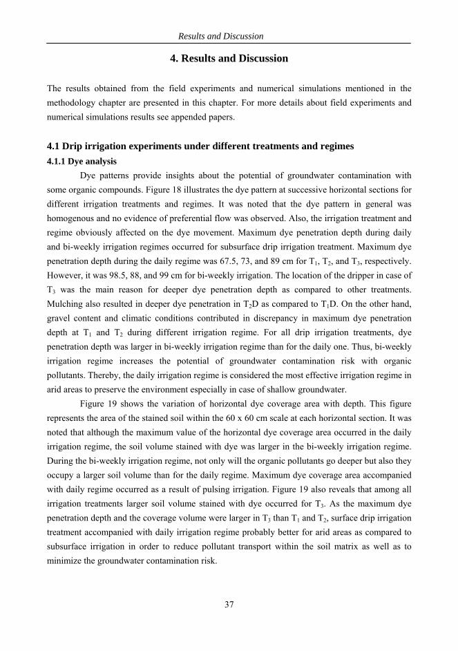
Results and Discussion

4. Results and Discussion

The results obtained from the field experiments and numerical simulations mentioned in the

methodology chapter are presented in this chapter. For more details about field experiments and

numerical simulations results see appended papers.

4.1 Drip irrigation experiments under different treatments and regimes 4.1.1 Dye analysis

Dye patterns provide insights about the potential of groundwater contamination with

some organic compounds. Figure 18 illustrates the dye pattern at successive horizontal sections for

different irrigation treatments and regimes. It was noted that the dye pattern in general was

homogenous and no evidence of preferential flow was observed. Also, the irrigation treatment and

regime obviously affected on the dye movement. Maximum dye penetration depth during daily

and bi-weekly irrigation regimes occurred for subsurface drip irrigation treatment. Maximum dye

penetration depth during the daily regime was 67.5, 73, and 89 cm for T1, T2, and T3, respectively.

However, it was 98.5, 88, and 99 cm for bi-weekly irrigation. The location of the dripper in case of

T3 was the main reason for deeper dye penetration depth as compared to other treatments.

Mulching also resulted in deeper dye penetration in T2D as compared to T1D. On the other hand,

gravel content and climatic conditions contributed in discrepancy in maximum dye penetration

depth at T1 and T2 during different irrigation regime. For all drip irrigation treatments, dye

penetration depth was larger in bi-weekly irrigation regime than for the daily one. Thus, bi-weekly

irrigation regime increases the potential of groundwater contamination risk with organic

pollutants. Thereby, the daily irrigation regime is considered the most effective irrigation regime in

arid areas to preserve the environment especially in case of shallow groundwater.

Figure 19 shows the variation of horizontal dye coverage area with depth. This figure

represents the area of the stained soil within the 60 x 60 cm scale at each horizontal section. It was

noted that although the maximum value of the horizontal dye coverage area occurred in the daily

irrigation regime, the soil volume stained with dye was larger in the bi-weekly irrigation regime.

During the bi-weekly irrigation regime, not only will the organic pollutants go deeper but also they

occupy a larger soil volume than for the daily regime. Maximum dye coverage area accompanied

with daily regime occurred as a result of pulsing irrigation. Figure 19 also reveals that among all

irrigation treatments larger soil volume stained with dye occurred for T3. As the maximum dye

penetration depth and the coverage volume were larger in T3 than T1 and T2, surface drip irrigation

treatment accompanied with daily irrigation regime probably better for arid areas as compared to

subsurface irrigation in order to reduce pollutant transport within the soil matrix as well as to

minimize the groundwater contamination risk.

37

Results and Discussion

Fig. 18, Dye pattern variation with depth. All sections are 60 cm long and 60 cm wide with dripper

in the center (no dye was observed outside the 60 x 60 cm scale).

38

Results and Discussion

-100-90-80-70-60-50-40-30-20-10

00 300 600 900 1200 1500 1800 2100

T1 DT1 WT2 DT2 WT3 DT3 W

Fig. 19, Dye covered area vs. depth for different treatment.

4.1.2 Soil water distribution Figure 20 shows soil water content maps for the different drip irrigation treatments and

regimes after 72 h from the commencement of irrigation. These maps represent water content

distribution within one half of the wetted zone at a vertical section passing through the dripper

perpendicular to the drip tubing. Water content maps revealed that for all treatments, soil wetting

due to the upward movement of water by capillary action was less pronounced during the bi-

weekly irrigation regime as compared to the daily one. In addition, soil water content was higher

for the daily regime as compared to those in the bi-weekly regime. This was mainly attributed to

the longer redistribution stage in case of the bi-weekly regime. This leads to lower soil moisture

content levels especially at the top soil layer as compared to the case of the daily regime.

Therefore, daily irrigation regime is recommended to keep the top soil layer moist with adequate

amount of soil water as compared to bi-weekly regime. A higher soil moisture content level and

larger lateral (radial) extension of the wetted zone were recorded during T2 as compared to T1 and

T3. This was mainly due to the mulching treatment. Covering the land by plastic mulch prevented

the evaporation and kept the soil water content at higher levels especially at the surface soil layer.

However, in T1, the evaporation showed a significant effect on soil water content values at the top

soil layer. The evaporation was more pronounced at the soil surface far from the dripper. The

installation depth and soil evaporation, on the other hand, were the reasons for lower soil moisture

content at the soil surface in T3. Therefore, mulching treatment is considered as a suitable

treatment in arid regions as compared to other treatments not only to enrich soil water content

within the flow domain but also to increase the distance between the drip laterals (due to the large

lateral extension of the wetted zone). Although T2 leads to additional cost due to the mulching

procedure, the total cost of this treatment can be less than other treatments due to the reduction in

drip lateral number.

39

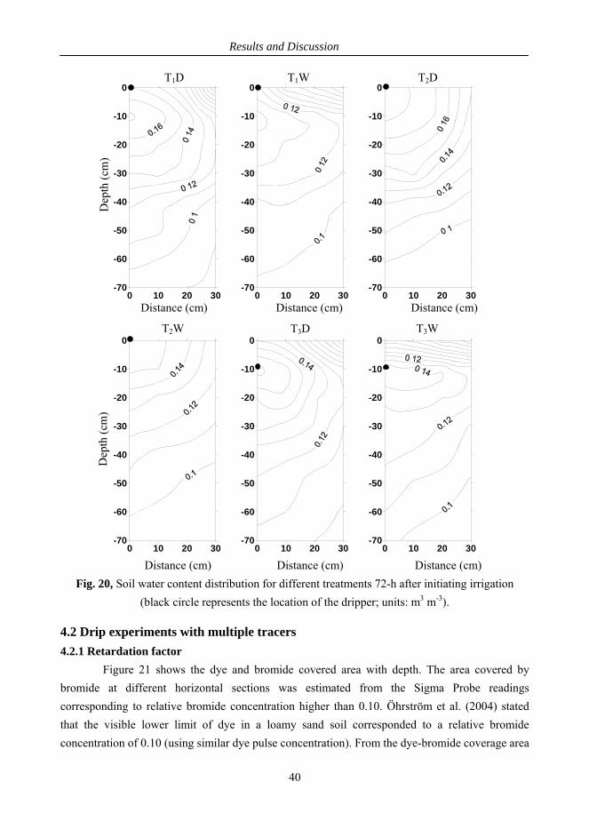
Results and Discussion

-70

-60

-50

-40

-30

-20

-10

0

0 10 20 30 -70

-60

-50

-40

-30

-20

-10

0

0 10 20 30 -70

-60

-50

-40

-30

-20

-10

0

0 10 20 30 Distance (cm) Distance (cm) Distance (cm)

0 10 20 30-70

-60

-50

-40

-30

-20

-10

0

-70

-60

-50

-40

-30

-20

-10

0

0 10 20 30 -70

-60

-50

-40

-30

-20

-10

0

Dep

th (

cm)

D

epth

(cm

)

T1W T2D T1D

T3D T3WT2W

0 10 20 30 Distance (cm) Distance (cm) Distance (cm)

Fig. 20, Soil water content distribution for different treatments 72-h after initiating irrigation

(black circle represents the location of the dripper; units: m3 m-3).

4.2 Drip experiments with multiple tracers 4.2.1 Retardation factor

Figure 21 shows the dye and bromide covered area with depth. The area covered by

bromide at different horizontal sections was estimated from the Sigma Probe readings

corresponding to relative bromide concentration higher than 0.10. Öhrström et al. (2004) stated

that the visible lower limit of dye in a loamy sand soil corresponded to a relative bromide

concentration of 0.10 (using similar dye pulse concentration). From the dye-bromide coverage area

40

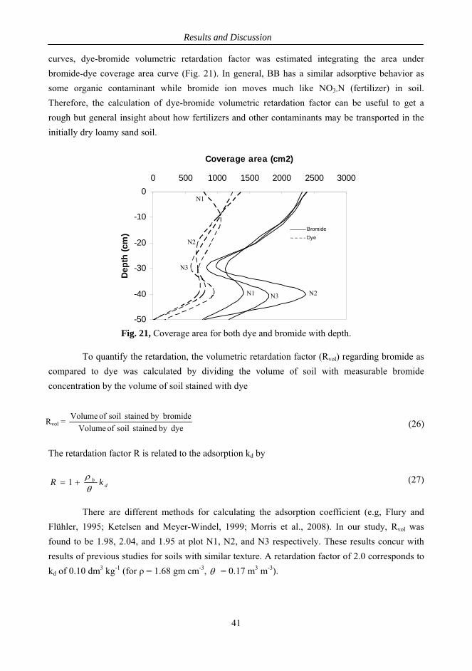
Results and Discussion

curves, dye-bromide volumetric retardation factor was estimated integrating the area under

bromide-dye coverage area curve (Fig. 21). In general, BB has a similar adsorptive behavior as

some organic contaminant while bromide ion moves much like NO3-N (fertilizer) in soil.

Therefore, the calculation of dye-bromide volumetric retardation factor can be useful to get a

rough but general insight about how fertilizers and other contaminants may be transported in the

initially dry loamy sand soil.

Coverage area (cm2)

-50

-40

-30

-20

-10

00 500 1000 1500 2000 2500 3000

Dept

h (c

m)

BromideDye

N3

N2

N1

N1 N2N3

Fig. 21, Coverage area for both dye and bromide with depth.

To quantify the retardation, the volumetric retardation factor (Rvol) regarding bromide as

compared to dye was calculated by dividing the volume of soil with measurable bromide

concentration by the volume of soil stained with dye

Rvol =

dyeby stained soil of Volume

bromideby stained soil of Volume (26)

The retardation factor R is related to the adsorption kd by

db kR

1 (27)

There are different methods for calculating the adsorption coefficient (e.g, Flury and

Flühler, 1995; Ketelsen and Meyer-Windel, 1999; Morris et al., 2008). In our study, Rvol was

found to be 1.98, 2.04, and 1.95 at plot N1, N2, and N3 respectively. These results concur with

results of previous studies for soils with similar texture. A retardation factor of 2.0 corresponds to

kd of 0.10 dm3 kg-1 (for ρ = 1.68 gm cm-3, = 0.17 m3 m-3).

41

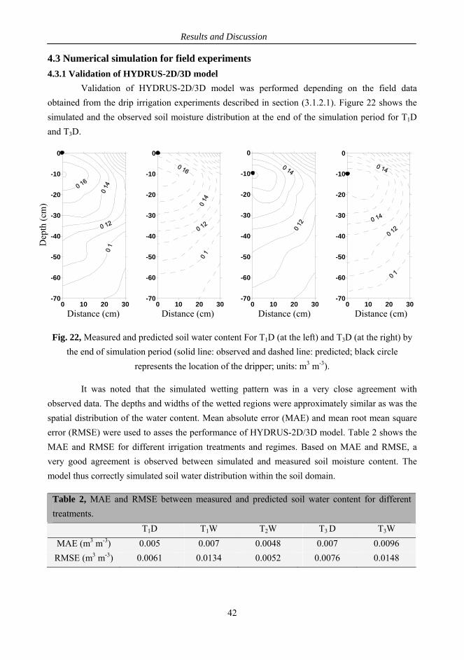
Results and Discussion

4.3 Numerical simulation for field experiments

4.3.1 Validation of HYDRUS-2D/3D model Validation of HYDRUS-2D/3D model was performed depending on the field data

obtained from the drip irrigation experiments described in section (3.1.2.1). Figure 22 shows the

simulated and the observed soil moisture distribution at the end of the simulation period for T1D

and T3D.

0 10 20 30-70

-60

-50

-40

-30

-20

-10

0

0 10 20 30-70

-60

-50

-40

-30

-20

-10

0

0 10 20 30-70

-60

-50

-40

-30

-20

-10

0

0 10 20 30-70

-60

-50

-40

-30

-20

-10

0

Dep

th (

cm)

Distance (cm) Distance (cm) Distance (cm) Distance (cm) Fig. 22, Measured and predicted soil water content For T1D (at the left) and T3D (at the right) by

the end of simulation period (solid line: observed and dashed line: predicted; black circle

represents the location of the dripper; units: m3 m-3).

It was noted that the simulated wetting pattern was in a very close agreement with

observed data. The depths and widths of the wetted regions were approximately similar as was the

spatial distribution of the water content. Mean absolute error (MAE) and mean root mean square

error (RMSE) were used to asses the performance of HYDRUS-2D/3D model. Table 2 shows the

MAE and RMSE for different irrigation treatments and regimes. Based on MAE and RMSE, a

very good agreement is observed between simulated and measured soil moisture content. The

model thus correctly simulated soil water distribution within the soil domain.

Table 2, MAE and RMSE between measured and predicted soil water content for different

treatments. T1D T1W T2W T3 D T3W

MAE (m3 m-3) 0.005 0.007 0.0048 0.007 0.0096

RMSE (m3 m-3) 0.0061 0.0134 0.0052 0.0076 0.0148

42

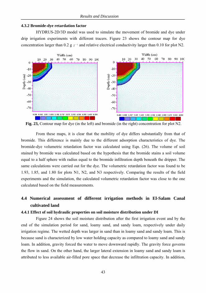
Results and Discussion

4.3.2 Bromide-dye retardation factor HYDRUS-2D/3D model was used to simulate the movement of bromide and dye under

drip irrigation experiments with different tracers. Figure 23 shows the contour map for dye

concentration larger than 0.2 g and relative electrical conductivity larger than 0.10 for plot N2. 1l

Fig. 23, Contour map for dye (in the left) and bromide (in the right) concentration for plot N2.

From these maps, it is clear that the mobility of dye differs substantially from that of

bromide. This difference is mainly due to the different adsorption characteristics of dye. The

bromide-dye volumetric retardation factor was calculated using Eqn. (26). The volume of soil

stained by bromide was calculated based on the hypothesis that the bromide stains a soil volume

equal to a half sphere with radius equal to the bromide infiltration depth beneath the dripper. The

same calculations were carried out for the dye. The volumetric retardation factor was found to be

1.93, 1.85, and 1.80 for plots N1, N2, and N3 respectively. Comparing the results of the field

experiments and the simulation, the calculated volumetric retardation factor was close to the one

calculated based on the field measurements.

4.4 Numerical assessment of different irrigation methods in El-Salam Canal cultivated land

4.4.1 Effect of soil hydraulic properties on soil moisture distribution under DI Figure 24 shows the soil moisture distribution after the first irrigation event and by the

end of the simulation period for sand, loamy sand, and sandy loam, respectively under daily

irrigation regime. The wetted depth was larger in sand than in loamy sand and sandy loam. This is

because sand is characterized by low water holding capacity as compared to loamy sand and sandy

loam. In addition, gravity forced the water to move downward rapidly. The gravity force governs

the flow in sand. On the other hand, the larger lateral extension in loamy sand and sandy loam is

attributed to less available air-filled pore space that decrease the infiltration capacity. In addition,

43

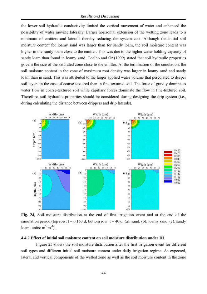
Results and Discussion

the lower soil hydraulic conductivity limited the vertical movement of water and enhanced the

possibility of water moving laterally. Larger horizontal extension of the wetting zone leads to a

minimum of emitters and laterals thereby reducing the system cost. Although the initial soil

moisture content for loamy sand was larger than for sandy loam, the soil moisture content was

higher in the sandy loam close to the emitter. This was due to the higher water holding capacity of

sandy loam than found in loamy sand. Coelho and Or (1999) stated that soil hydraulic properties

govern the size of the saturated zone close to the emitter. At the termination of the simulation, the

soil moisture content in the zone of maximum root density was larger in loamy sand and sandy

loam than in sand. This was attributed to the larger applied water volume that percolated to deeper

soil layers in the case of coarse-textured than in fine-textured soil. The force of gravity dominates

water flow in coarse-textured soil while capillary forces dominate the flow in fine-textured soil.

Therefore, soil hydraulic properties should be considered during designing the drip system (i.e.,

during calculating the distance between drippers and drip laterals).

Width (cm) Width (cm) Width (cm)

(a)(c)(b)

Dep

th (

cm)

Width (cm) Width (cm) Width (cm)

(b)(a) (c)

Dep

th (

cm)

Fig. 24, Soil moisture distribution at the end of first irrigation event and at the end of the

simulation period (top row: t = 0.153 d; bottom row: t = 40 d; (a): sand; (b): loamy sand, (c): sandy

loam; units: m3 m-3).

4.4.2 Effect of initial soil moisture content on soil moisture distribution under DI Figure 25 shows the soil moisture distribution after the first irrigation event for different

soil types and different initial soil moisture content under daily irrigation regime. As expected,

lateral and vertical components of the wetted zone as well as the soil moisture content in the zone

44

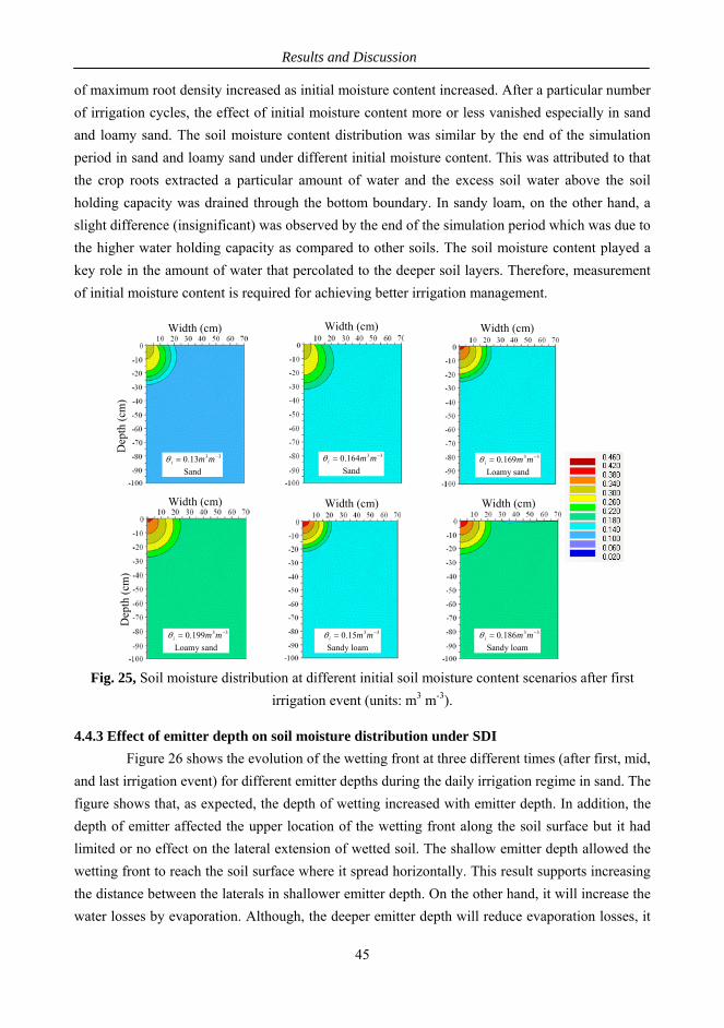
Results and Discussion

of maximum root density increased as initial moisture content increased. After a particular number

of irrigation cycles, the effect of initial moisture content more or less vanished especially in sand

and loamy sand. The soil moisture content distribution was similar by the end of the simulation

period in sand and loamy sand under different initial moisture content. This was attributed to that

the crop roots extracted a particular amount of water and the excess soil water above the soil

holding capacity was drained through the bottom boundary. In sandy loam, on the other hand, a

slight difference (insignificant) was observed by the end of the simulation period which was due to

the higher water holding capacity as compared to other soils. The soil moisture content played a

key role in the amount of water that percolated to the deeper soil layers. Therefore, measurement

of initial moisture content is required for achieving better irrigation management.

Width (cm) Width (cm) Width (cm)

Dep

th (

cm)

33164.0 mmiSand

3313.0 mmiSand

33169.0 mmiLoamy sand

Width (cm) Width (cm) Width (cm)

Dep

th (

cm)

33199.0 mmi

Loamy sand

3315.0 mmiSandy loam

33186.0 mmiSandy loam

Fig. 25, Soil moisture distribution at different initial soil moisture content scenarios after first

irrigation event (units: m3 m-3).

4.4.3 Effect of emitter depth on soil moisture distribution under SDI Figure 26 shows the evolution of the wetting front at three different times (after first, mid,

and last irrigation event) for different emitter depths during the daily irrigation regime in sand. The

figure shows that, as expected, the depth of wetting increased with emitter depth. In addition, the

depth of emitter affected the upper location of the wetting front along the soil surface but it had

limited or no effect on the lateral extension of wetted soil. The shallow emitter depth allowed the

wetting front to reach the soil surface where it spread horizontally. This result supports increasing

the distance between the laterals in shallower emitter depth. On the other hand, it will increase the

water losses by evaporation. Although, the deeper emitter depth will reduce evaporation losses, it

45

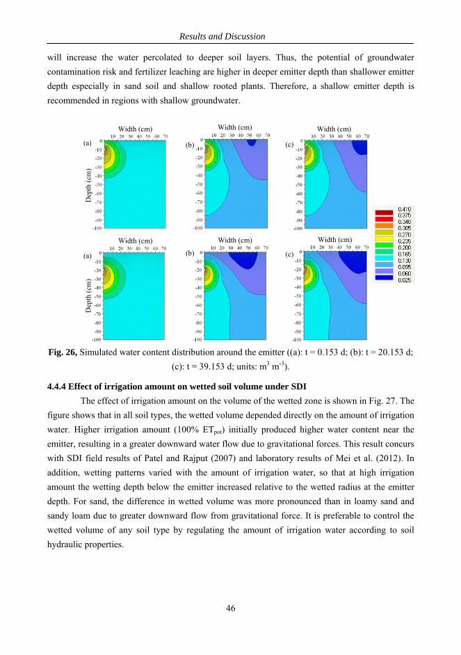
Results and Discussion

will increase the water percolated to deeper soil layers. Thus, the potential of groundwater

contamination risk and fertilizer leaching are higher in deeper emitter depth than shallower emitter

depth especially in sand soil and shallow rooted plants. Therefore, a shallow emitter depth is

recommended in regions with shallow groundwater.

Width (cm) Width (cm) Width (cm)

(a) (c)(b)

Dep

th (

cm)

Width (cm) Width (cm) Width (cm)

(b) (c)(a)

Dep

th (

cm)

Fig. 26, Simulated water content distribution around the emitter ((a): t = 0.153 d; (b): t = 20.153 d;

(c): t = 39.153 d; units: m3 m-3).

4.4.4 Effect of irrigation amount on wetted soil volume under SDI The effect of irrigation amount on the volume of the wetted zone is shown in Fig. 27. The

figure shows that in all soil types, the wetted volume depended directly on the amount of irrigation

water. Higher irrigation amount (100% ETpot) initially produced higher water content near the

emitter, resulting in a greater downward water flow due to gravitational forces. This result concurs

with SDI field results of Patel and Rajput (2007) and laboratory results of Mei et al. (2012). In

addition, wetting patterns varied with the amount of irrigation water, so that at high irrigation

amount the wetting depth below the emitter increased relative to the wetted radius at the emitter

depth. For sand, the difference in wetted volume was more pronounced than in loamy sand and

sandy loam due to greater downward flow from gravitational force. It is preferable to control the

wetted volume of any soil type by regulating the amount of irrigation water according to soil

hydraulic properties.

46

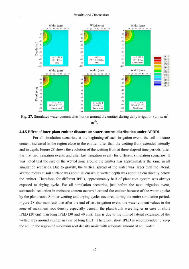
Results and Discussion

Width (cm) Width (cm) Width (cm)

Dep

th (

cm)

t = 0.13 d IW = 0.85 ETpot

Sand

t = 0.153 d IW = ETpot Loamy sand

t = 0.153 dIW = ETpot

Sand

Width (cm) Width (cm)

Width (cm)

Dep

th (

cm)

t = 0.13 d IW = 0.85 ETpot

Loamy sand

t = 0.13 d IW = 0.85 ETpot

Sand loam

t = 0.153 dIW = ETpot

Sandy loam

Fig. 27, Simulated water content distribution around the emitter during daily irrigation (units: m3

m-3).

4.4.5 Effect of inter-plant emitter distance on water content distribution under APRDI For all simulation scenarios, at the beginning of each irrigation event, the soil moisture

content increased in the region close to the emitter, after that, the wetting front extended laterally

and in depth. Figure 28 shows the evolution of the wetting front at three elapsed time periods (after

the first two irrigation events and after last irrigation event) for different simulation scenarios. It

was noted that the size of the wetted zone around the emitter was approximately the same in all

simulation scenarios. Due to gravity, the vertical spread of the water was larger than the lateral.

Wetted radius at soil surface was about 20 cm while wetted depth was about 25 cm directly below

the emitter. Therefore, for different IPED, approximately half of plant root system was always

exposed to drying cycle. For all simulation scenarios, just before the next irrigation event,

substantial reduction in moisture content occurred around the emitter because of the water uptake

by the plant roots. Similar wetting and drying cycles occurred during the entire simulation period.

Figure 28 also manifests that after the end of last irrigation event, the water content values in the

zone of maximum root density especially beneath the plant trunk were higher in case of short

IPED (20 cm) than long IPED (30 and 40 cm). This is due to the limited lateral extension of the

wetted area around emitter in case of long IPED. Therefore, short IPED is recommended to keep

the soil in the region of maximum root density moist with adequate amount of soil water.

47

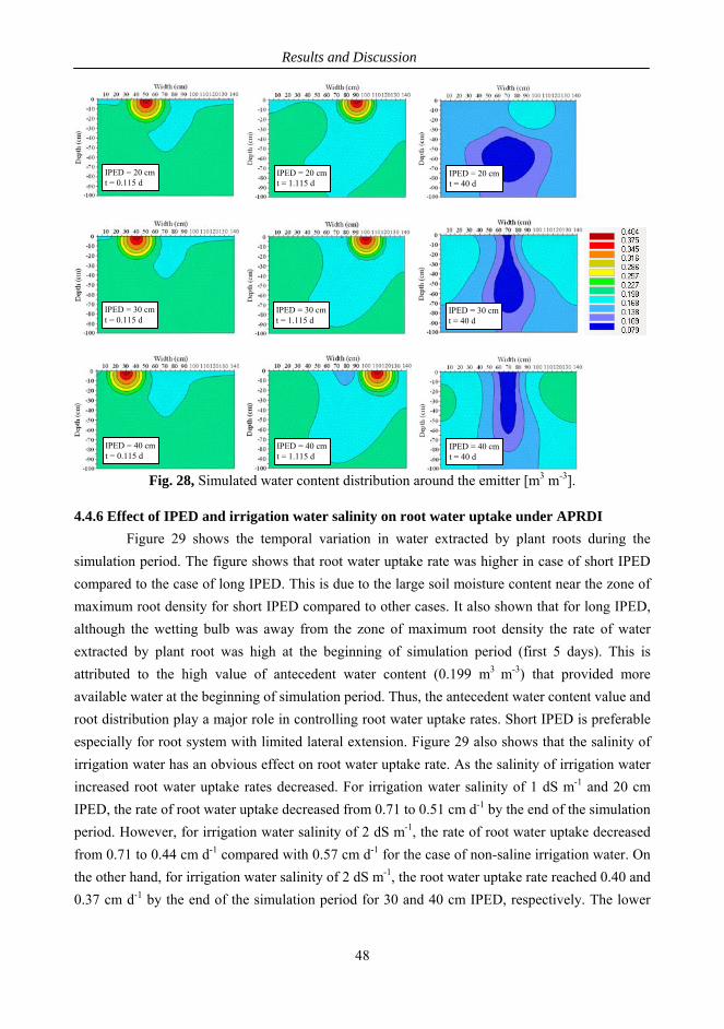
Results and Discussion

IPED = 20 cmt = 1.115 d

IPED = 20 cmt = 40 d

IPED = 20 cm t = 0.115 d

IPED = 30 cm t = 0.115 d

IPED = 30 cmt = 1.115 d

IPED = 30 cmt = 40 d

IPED = 40 cm t = 0.115 d

IPED = 40 cmt = 1.115 d

IPED = 40 cmt = 40 d

Fig. 28, Simulated water content distribution around the emitter [m3 m-3].

4.4.6 Effect of IPED and irrigation water salinity on root water uptake under APRDI Figure 29 shows the temporal variation in water extracted by plant roots during the

simulation period. The figure shows that root water uptake rate was higher in case of short IPED

compared to the case of long IPED. This is due to the large soil moisture content near the zone of

maximum root density for short IPED compared to other cases. It also shown that for long IPED,

although the wetting bulb was away from the zone of maximum root density the rate of water

extracted by plant root was high at the beginning of simulation period (first 5 days). This is

attributed to the high value of antecedent water content (0.199 m3 m-3) that provided more

available water at the beginning of simulation period. Thus, the antecedent water content value and

root distribution play a major role in controlling root water uptake rates. Short IPED is preferable

especially for root system with limited lateral extension. Figure 29 also shows that the salinity of

irrigation water has an obvious effect on root water uptake rate. As the salinity of irrigation water

increased root water uptake rates decreased. For irrigation water salinity of 1 dS m-1 and 20 cm

IPED, the rate of root water uptake decreased from 0.71 to 0.51 cm d-1 by the end of the simulation

period. However, for irrigation water salinity of 2 dS m-1, the rate of root water uptake decreased

from 0.71 to 0.44 cm d-1 compared with 0.57 cm d-1 for the case of non-saline irrigation water. On

the other hand, for irrigation water salinity of 2 dS m-1, the root water uptake rate reached 0.40 and

0.37 cm d-1 by the end of the simulation period for 30 and 40 cm IPED, respectively. The lower

48

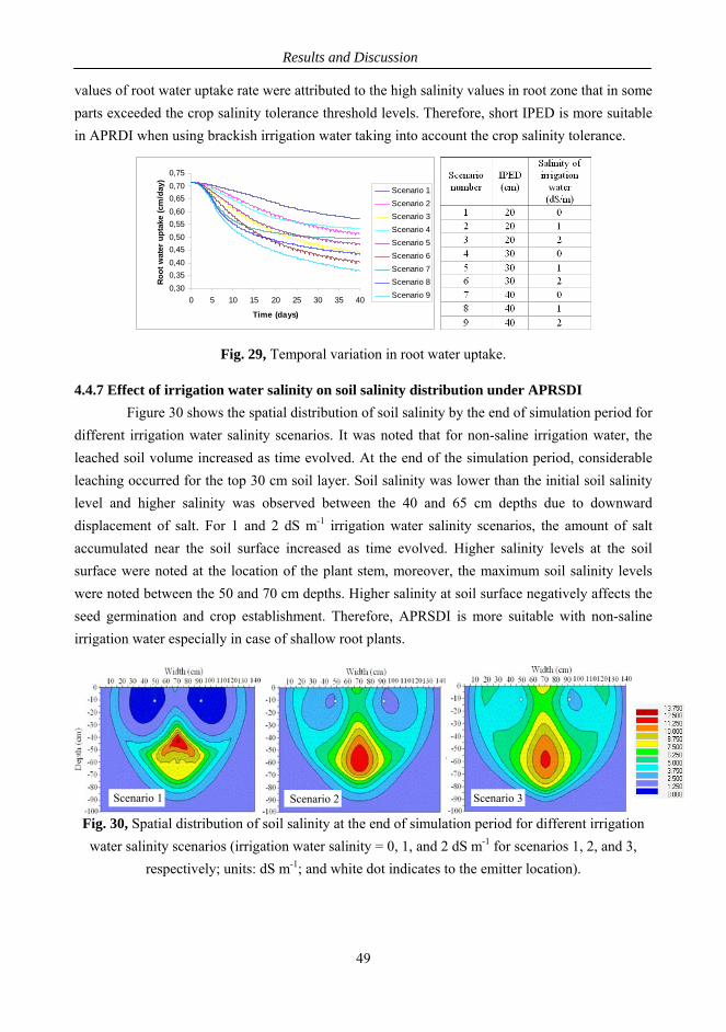
Results and Discussion

values of root water uptake rate were attributed to the high salinity values in root zone that in some

parts exceeded the crop salinity tolerance threshold levels. Therefore, short IPED is more suitable

in APRDI when using brackish irrigation water taking into account the crop salinity tolerance.

0,300,350,400,450,500,550,600,650,700,75

0 5 10 15 20 25 30 35 40

Time (days)

Root

wat

er u

ptak

e (c

m/d

ay)

Scenario 1Scenario 2Scenario 3Scenario 4Scenario 5Scenario 6Scenario 7Scenario 8Scenario 9

Fig. 29, Temporal variation in root water uptake.

4.4.7 Effect of irrigation water salinity on soil salinity distribution under APRSDI Figure 30 shows the spatial distribution of soil salinity by the end of simulation period for

different irrigation water salinity scenarios. It was noted that for non-saline irrigation water, the

leached soil volume increased as time evolved. At the end of the simulation period, considerable

leaching occurred for the top 30 cm soil layer. Soil salinity was lower than the initial soil salinity

level and higher salinity was observed between the 40 and 65 cm depths due to downward

displacement of salt. For 1 and 2 dS m-1 irrigation water salinity scenarios, the amount of salt

accumulated near the soil surface increased as time evolved. Higher salinity levels at the soil

surface were noted at the location of the plant stem, moreover, the maximum soil salinity levels

were noted between the 50 and 70 cm depths. Higher salinity at soil surface negatively affects the

seed germination and crop establishment. Therefore, APRSDI is more suitable with non-saline

irrigation water especially in case of shallow root plants.

Scenario 1 Scenario 3Scenario 2

Fig. 30, Spatial distribution of soil salinity at the end of simulation period for different irrigation

water salinity scenarios (irrigation water salinity = 0, 1, and 2 dS m-1 for scenarios 1, 2, and 3,

respectively; units: dS m-1; and white dot indicates to the emitter location).

49

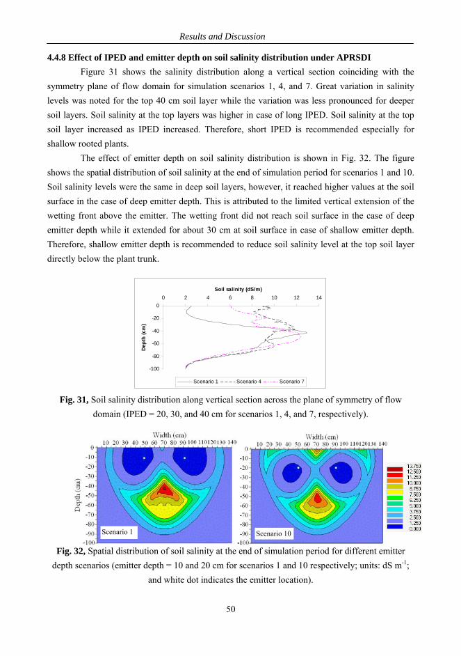
Results and Discussion

4.4.8 Effect of IPED and emitter depth on soil salinity distribution under APRSDI Figure 31 shows the salinity distribution along a vertical section coinciding with the

symmetry plane of flow domain for simulation scenarios 1, 4, and 7. Great variation in salinity

levels was noted for the top 40 cm soil layer while the variation was less pronounced for deeper

soil layers. Soil salinity at the top layers was higher in case of long IPED. Soil salinity at the top

soil layer increased as IPED increased. Therefore, short IPED is recommended especially for

shallow rooted plants.

The effect of emitter depth on soil salinity distribution is shown in Fig. 32. The figure

shows the spatial distribution of soil salinity at the end of simulation period for scenarios 1 and 10.

Soil salinity levels were the same in deep soil layers, however, it reached higher values at the soil

surface in the case of deep emitter depth. This is attributed to the limited vertical extension of the

wetting front above the emitter. The wetting front did not reach soil surface in the case of deep

emitter depth while it extended for about 30 cm at soil surface in case of shallow emitter depth.

Therefore, shallow emitter depth is recommended to reduce soil salinity level at the top soil layer

directly below the plant trunk.

-100

-80

-60

-40

-20

00 2 4 6 8 10 12 14

Soil salinity (dS/m)

Dept

h (c

m)

Scenario 1 Scenario 4 Scenario 7

Fig. 31, Soil salinity distribution along vertical section across the plane of symmetry of flow

domain (IPED = 20, 30, and 40 cm for scenarios 1, 4, and 7, respectively).

Scenario 1 Scenario 10

Fig. 32, Spatial distribution of soil salinity at the end of simulation period for different emitter

depth scenarios (emitter depth = 10 and 20 cm for scenarios 1 and 10 respectively; units: dS m-1;

and white dot indicates the emitter location).

50

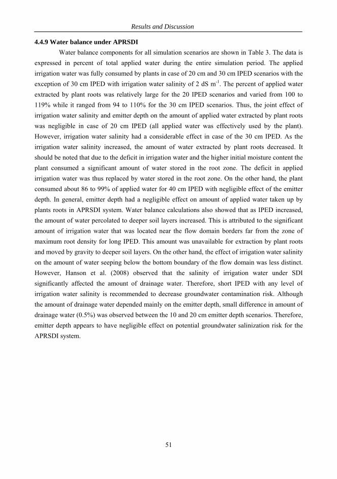
Results and Discussion

4.4.9 Water balance under APRSDI Water balance components for all simulation scenarios are shown in Table 3. The data is

expressed in percent of total applied water during the entire simulation period. The applied

irrigation water was fully consumed by plants in case of 20 cm and 30 cm IPED scenarios with the

exception of 30 cm IPED with irrigation water salinity of 2 dS m-1. The percent of applied water

extracted by plant roots was relatively large for the 20 IPED scenarios and varied from 100 to

119% while it ranged from 94 to 110% for the 30 cm IPED scenarios. Thus, the joint effect of

irrigation water salinity and emitter depth on the amount of applied water extracted by plant roots

was negligible in case of 20 cm IPED (all applied water was effectively used by the plant).

However, irrigation water salinity had a considerable effect in case of the 30 cm IPED. As the

irrigation water salinity increased, the amount of water extracted by plant roots decreased. It

should be noted that due to the deficit in irrigation water and the higher initial moisture content the

plant consumed a significant amount of water stored in the root zone. The deficit in applied

irrigation water was thus replaced by water stored in the root zone. On the other hand, the plant

consumed about 86 to 99% of applied water for 40 cm IPED with negligible effect of the emitter

depth. In general, emitter depth had a negligible effect on amount of applied water taken up by

plants roots in APRSDI system. Water balance calculations also showed that as IPED increased,

the amount of water percolated to deeper soil layers increased. This is attributed to the significant

amount of irrigation water that was located near the flow domain borders far from the zone of

maximum root density for long IPED. This amount was unavailable for extraction by plant roots

and moved by gravity to deeper soil layers. On the other hand, the effect of irrigation water salinity

on the amount of water seeping below the bottom boundary of the flow domain was less distinct.

However, Hanson et al. (2008) observed that the salinity of irrigation water under SDI

significantly affected the amount of drainage water. Therefore, short IPED with any level of

irrigation water salinity is recommended to decrease groundwater contamination risk. Although

the amount of drainage water depended mainly on the emitter depth, small difference in amount of

drainage water (0.5%) was observed between the 10 and 20 cm emitter depth scenarios. Therefore,

emitter depth appears to have negligible effect on potential groundwater salinization risk for the

APRSDI system.

51

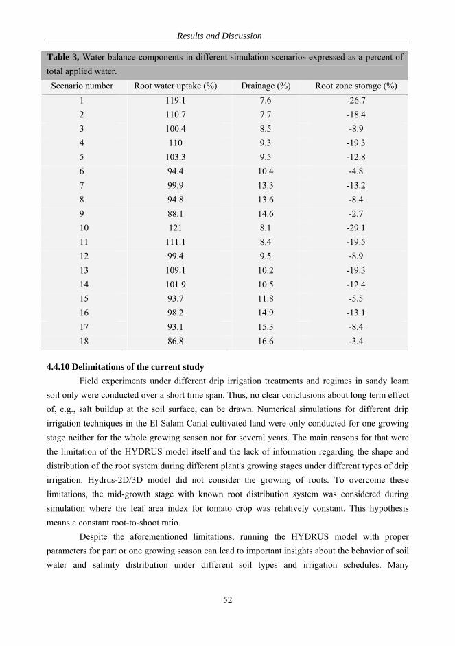
Results and Discussion

Table 3, Water balance components in different simulation scenarios expressed as a percent of

total applied water.

Scenario number Root water uptake (%) Drainage (%) Root zone storage (%)

1 119.1 7.6 -26.7

2 110.7 7.7 -18.4

3 100.4 8.5 -8.9

4 110 9.3 -19.3

5 103.3 9.5 -12.8

6 94.4 10.4 -4.8

7 99.9 13.3 -13.2

8 94.8 13.6 -8.4

9 88.1 14.6 -2.7

10 121 8.1 -29.1

11 111.1 8.4 -19.5

12 99.4 9.5 -8.9

13 109.1 10.2 -19.3

14 101.9 10.5 -12.4

15 93.7 11.8 -5.5

16 98.2 14.9 -13.1

17 93.1 15.3 -8.4

18 86.8 16.6 -3.4

4.4.10 Delimitations of the current study

Field experiments under different drip irrigation treatments and regimes in sandy loam

soil only were conducted over a short time span. Thus, no clear conclusions about long term effect

of, e.g., salt buildup at the soil surface, can be drawn. Numerical simulations for different drip

irrigation techniques in the El-Salam Canal cultivated land were only conducted for one growing

stage neither for the whole growing season nor for several years. The main reasons for that were

the limitation of the HYDRUS model itself and the lack of information regarding the shape and

distribution of the root system during different plant's growing stages under different types of drip

irrigation. Hydrus-2D/3D model did not consider the growing of roots. To overcome these

limitations, the mid-growth stage with known root distribution system was considered during

simulation where the leaf area index for tomato crop was relatively constant. This hypothesis

means a constant root-to-shoot ratio.

Despite the aforementioned limitations, running the HYDRUS model with proper

parameters for part or one growing season can lead to important insights about the behavior of soil

water and salinity distribution under different soil types and irrigation schedules. Many

52

Results and Discussion

53

recommendations that can be practiced in the El-Salam Canal Cultivated land were presented and

discussed in the appended papers. To maximize the benefits of the current study long term field

experiments in the El-Salam Canal cultivated land for at least one of the simulated scenarios are

recommended to be implemented and a comparison between field and numerical simulation results

should be conducted.

Shifting from surface irrigation systems to drip irrigation will lead to reduction in

irrigation water. Modern irrigation techniques, e.g. sprinkler or drip irrigation, consume an average

amount of water of 1.40 m3 m-2 y-1 as compared to an average of 3.50 m3 m-2 y-1 in surface

irrigation methods. Nowadays, the limitation of implementing drip irrigation techniques in small

farms (i.e., 1 to 2 feddan) in El-Salam Canal cultivated land arises from the relatively high initial

cost of these techniques. Therefore, the Egyptian government should financially support the small

land holders in this regard (i.e., giving loans which can be long-term reimbursement without

interest) to motivate them to use these systems. On the other hand, there is no need for financial

support for investors who own larger farms as the initial cost will be less in this case.

Summary and Conclusion

5. Summary and Conclusion

Improving irrigation practices and optimal exploitation of available water resources are vital issues facing water scarcity and similar problems in arid and semiarid countries (e.g., Egypt and Tunisia). In these countries, the use of brackish irrigation water is often associated by soil salinization risk and soil degradation due to mismanagement and improper irrigation methods. In the present study, field, laboratory, and numerical experiments were conducted to investigate the effect of using brackish irrigation water on soil salinity distribution and groundwater salinization risk under different treatments and techniques of water conservation practice in agriculture (i.e., drip irrigation). In addition, the influence of irrigation amount, emitter depth, irrigation regime, and soil hydraulic properties on irrigation efficiency and soil water distribution within the flow domain were also investigated. The conducted field experiments were divided into two sets, while the numerical simulations were carried out for four different drip irrigation techniques. The laboratory experiments were conducted for collected soil samples to provide the required data for simulation implementation and analysis. The first set of field experiments was carried out in sandy loam soil in Tunisia with a mixture of brackish irrigation water and dye tracer to explore soil water and salinity distribution under three different treatments of drip irrigation with two irrigation regimes, furthermore, to validate the numerical model (i.e., HYDRUS-2D/3D). The three treatments were surface drip irrigation without and with plastic mulch and subsurface drip irrigation with drip tube 10 cm below soil surface, while, daily and bi-weekly irrigation regimes were considered during performing each treatment. The second set of field experiments was conducted using surface drip irrigation with a mixture of brackish water, BB dye, and potassium bromide in loamy sand soil in Tunisia. The main goal of this set of experiment was to investigate the mobility of both tracers (i.e., dye and bromide) as an indicator for the movement of fertilizers and organic pollutants through the field soil under surface drip irrigation. Numerical simulations, on the other hand, were implemented to investigate the effect of geometric design aspects, irrigation regime, irrigation amount, and salinity of irrigation water on soil water and salinity distribution as well as irrigation efficiency for different soil types in the El-Salam Canal project region, Egypt under different drip irrigation techniques. These techniques were surface drip irrigation, subsurface drip irrigation, alternate partial root-zone surface drip irrigation, and alternate partial root-zone surface drip irrigation.

Field results showed that mulching treatment with daily irrigation regime reduces groundwater contamination risk and improves soil water status within the soil domain in sandy loam soil over other drip irrigation treatments and regimes. Also, the simulated wetting pattern by HYDRUS-2D/3D was in a very close agreement with the observed data. In addition, the bromide flow in different pathways as compared to dye. Therefore, fertilizers can move deeper than organic pollutants under surface drip irrigation in initially dry loamy sand soil. On the other hand,

54

Summary and Conclusion

55

numerical simulations for El-Salam Canal cultivated land showed that under surface drip irrigation the wetted depth was larger in sand than in loamy sand and sandy loam and the soil moisture content gradient in the vertical direction was steeper for sandy loam than for sand and loamy sand while the soil moisture content gradient in the horizontal direction was steeper in sand. Therefore, soil hydraulic properties should be considered during designing the drip system. Simulation results for subsurface drip irrigation showed that the potential groundwater contamination risk and fertilizer leaching are higher in deeper emitter depth than shallower emitter depth especially in sand soil and shallow rooted plants. Therefore, shallow emitter depth is recommended in regions with shallow groundwater. Larger irrigation amount (100% of ETpot), on the other hand, initially produced higher water content near the emitter, resulting in a greater downward water flow due to gravitational forces regardless of emitter depth. Therefore, it is preferable to control the wetted volume of any soil type by regulating the amount of irrigation water according to soil hydraulic properties. Simulation results also demonstrated that short inter-plant emitter distances is appropriate to sustain a considerable amount of soil moisture in the zone of maximum root density under alternate partial root-zone surface and subsurface drip irrigation (APRDI and APRSDI, respectively). Thereby, higher root water uptake rates were recorded with short IPED. Thus short IPED is preferable especially for root system with limited lateral extension. Salinity results showed that higher salinity levels at the soil surface at the location of the plant trunk under APRSDI were occurred for irrigation water salinity of 1 and 2 dS m-1. Therefore, APRSDI is more suitable with non-saline irrigation water, especially for shallow rooted plants. However, short IPED and shallow emitter depth are recommended for reducing soil salinity below the plant trunk in case of using brackish irrigation water. Based on the above, HYDRUS-2D/3D can be used as a fast and cost effective assessment tool for water flow and salt movement under different treatments and techniques of drip irrigation.

Overall, I believe that the present work provides a clear visualization of soil water and salinity distribution as well as pollutant transport under different drip irrigation techniques with brackish water in different types of soil in arid and semiarid regions, especially, in the new reclaimed areas within the El-Salam Canal command. Fortunately, the trend of the Egyptian government nowadays is to develop and establish new communities in Sinai to add more stability along the Egyptian borders. Therefore, this visualization can generally enhance the socioeconomic development and mitigate the poverty level of the El-Salam Canal command region specifically and of Sinai Peninsula generally which was forgotten during the past decades.

References

6- References

Abdel-Azim, R., and M. N. Allam. 2004. Agricultural drainage water reuse in Egypt: strategic issues and mitigation measures. Non-conventional water use workshop, Cairo, Egypt, pp 105-117.

Abdin, A., and I. Gaafar. 2009. Rational water use in Egypt. Technological Perspectives for Rational Use of Water Resources in the Mediterranean Region Options Méditerranéennes, Series A (Mediterranean Seminars), No. 88. ISSN 1016-121X.

Abou Lila, T. S., M. I. Balah, and Y. A. Hamed. 2005. Solute infiltration and spatial salinity distribution behavior for the main soil types at El-Salam Canal project cultivated land. Port Said Eng. Res. J. 9: 242-253.

Abou-Zeid, M. 1988. Egypt’s policies to use low-quality water for irrigation. Proc. Symp. Reuse of Low-quality Water for Irrigation. Water Research Center, Cairo, Egypt, pp 21-36.

Ajdary, K., D. K. Singh, A. K. Singh, and M. Khanna. 2007. Modelling of nitrogen leaching from experimental onion field under drip fertigation. Agric. Water Manage. 89: 15-28.

Allam, M. N., and G. I. Allam. 2007. Water resources in Egypt: future challenges and opportunities. IWRA, Water International, 32(2): 205-218.

Allen, R., L. Pereira., D. Raes, and M. Smith, 1998. Crop Evapotranspiration, Guidelines for Computing Crop Water Requirements, FAO Irrigation and Drainage Paper No. 56. Rome, Italy.

Amer, M. H., and D. S. Alnagar. 1989. Fayoum pilot project for the reuse of drainage water for irrigation. In Reuse of Low Quality Water for Irrigation in Mediterranean Countries. R. Bouchet (ed.). Proc. Cairo/ Aswan Seminar.

Anderson, M. P. 1984. Movement of contaminants in groundwater: groundwater transport-advection and dispersion. In: Groundwater contamination. Studies in geophysics. National Academy, Washington, DC, pp 37-45.

Andreu, L., F. Moreno, N. J. Jarvis, and G. Vachaud. 1994. Application of the model MACRO to water movement and salt leaching in drained and irrigated marsh soils, Marismas, Spain. Agric. Water Manage. 25: 71-88.

Aquastat. 2005. FAO’s Information System on Water and Agriculture: Egypt. http://www.fao.org/nr/water/aquastat/countries/egypt/index.stm.

Assouline, S. 2002. The effect of microdrip and convential drip irrigation on water distribution and uptake. Soil Sci. Soc. Am. J. 66: 1630-1636.

Ayars, J., R. Hutmacher, and R. Schoneman. 1993. Long term use of saline water for irrigation. Irrig. Sci. 14: 27-34.

Ayars, J., R. Hutmacher, R. Schoneman, S. Vail, and D. Felleke. 1986. Drip irrigation of cotton with saline drainage water. Trans. Am. Soc. Agric. Eng., 29: 1668-1673.

56

References

Bajracharya, R., and S. Sharma. 2005. Influence of drip-irrigation method on performance and yields of cucumber and tomato. Kathmandu University J. Engineering and Technology, 1:1-7.

Bernstein, L., and L. Francois. 1973. Comparisons of drip, furrow, and sprinkler irrigation. Soil Sci., 115: 73-86.

Brandt, A., E. Bresler, N. Diner, I. Ben-Asher, J. Heller, and D. Goldgerg. 1971. Infiltration from a trickle source. I. Mathematical models. Soil Sci Soc Am Proc. 35: 675-682.

Bresler, E. 1977. Trickle-drip irrigation: principles and application to soil-water management. Adv Agron. 29: 343-393.

Brouwer, C., A. Goffeau, and M. Heibloem, 1985. Irrigation water management, Training manual No. 1: Introduction to irrigation. FAO, Rome.

Bufon, V. B., R. J. Lascano, C. Bednarz, J. D. Booker, and D. C. Gitz. 2011. Soil water content on drip irrigated cotton: comparison of measured and simulated values obtained with the Hydrus2-D model. Irrig. Sci. DOI 10.1007/s00271-011-0279-z.

Cavazza, L. 1988. Irrigation system and techniques for saline water. Seminars Mediterranean on Reuse of low quality water for irrigation in Mediterranean countries, pp 45-54.

Coelho, E. F., and D. Or. 1999. Root distribution and water uptake patterns of corn under surface and subsurface drip irrigation. Plant Soil 206: 123-136.

Colaizzi, P. D., F. R. Lamm, T. A. Howell, and S. R. Evett. 2006. Crop production comparison under various irrigation systems. In: Proc. Central Plains Irrigation Conference, Colby, KS., Feb. 21-22, 2006. Available from CPIA, 760 N. Thompson, Colby, KS. pp. 189-207.

Corwin, D. L., and S. M. Lesch. 2005. Characterizing soil spatial variability with apparent soil electrical conductivity. I. Survey protocols. Computer and Electronics in Agriculture. 46(1-3): 103-133.

Cote, C. M., K. L. Bristow, P. B. Charlesworth, F. J. Cook, and P. J. Thorburn. 2003. Analysis of soil wetting and solute transport in subsurface trickle irrigation. Irrig. Sci. J. 22: 143-156.

Cote, C., K. L. Bristow, E. J. Ford, K. Verburg, and B. Keating. 2001. Measurement of water and solute movement in large undisturbed soil cores: analysis of Macknade and Bundaderg data. CSIRO Land and Water, Technical Report 07/2001.

Crevoisier, D., Z. Popova, J.C. Mailhol, and P. Ruelle. 2008. Assessment and simulation of water and nitrogen transfer under furrow irrigation. Agric. Water Manage. 95: 354-366.

De Wit, C. T. 1958. Transpiration and crop yield. Versl. Landbouwk. Ondez., Wageningen University, The Netherlands, 64: 59-84.

El-Gamal, F. 2007. Use of non conventional water resources in irrigated agriculture. Water saving in Mediterranean agriculture and future research needs [Vol. 2]. Proceedings of the International Conference WASAMED Project (EU contract ICA3-CT-2002-10013), 2007/02/14-17, Valenzano, Italy.

57

References

Ellis, J., E. Kruse, A. McSay, C. Neale, and R. Horn. 1986. A comparison of five irrigation methods on onions. Hort. Sci. 21(6): 1349-1351.

Elmaloglou, S., and E. Diamantopoulos. 2010. Soil water dynamics under surface trickle irrigation as affected by soil hydraulic properties, discharge rate, dripper spacing and irrigation duration. Irrig. And Drain. 59: 254-263.

El-Quosy, D., A. Ahmed, and T. Ahmed. 1999. Water saving techniques- lessons learned from irrigation of agricultural land in Egypt. In: Proceedings of the VII Nile 1999 conference, Cairo March 15-19, 1999: EGY- 18: 1-18.

Feddes, R. A., P. J. Kowalik, and H. Zaradny. 1978. Simulation of FieldWater Use and Crop Yield. Simulation Monographs. Pudoc, Wageningen.

Fereres, E., and M. A. Soriano. 2007. Deficit irrigation for reducing agricultural water use. Journal of Experimental Botany, 58(2): 147-159.

Fereres, E., R. Cuevas, and F. Orgaz. 1985. Drip irrigation of cotton in southern spain. Proc. Third Drip/Trickle irrig. Congr., ASAE Publ. 10-85, ASAE, St. Joseph, Mi., pp: 185-192.

Flury, M., and H. Flühler. 1995. Tracer characteristics of Brilliant Blue FCF. Soil Sci. Soc. Am. J. 59, 22-27.

Gärdenäs, A., J. Hopmans, B. Hanson, and J. Simunek. 2005. Two-dimensional modeling of nitrate leaching for various fertigation Scenarios under micro-irrigation. Agric. Water Manage. 74: 219-242.

Gencoglan, C., H. Altunbey, and S. Gencoglan. 2006. Response of green beanto subsurface drip irrigation and partial root-zone drying irrigation. Agric. Water Manag. 84: 274-280.

Haijun, L., K. Yaohu, Y. Sumei, S. Zeqiang, L. Shiping, and W. Qinggai. 2011. Water Resource and Environmental Protection (ISWREP), 2011 International Symposium, China, pp 576-579.

Hamdy, A. 1999. Saline irrigation assessment and management for sustainable use. In: Proceedings on Non-Conventional Water Resources Practices and Management and Annual Meeting UWRM Sub- Network Partners IAV Hassan II, Rabat, Morocco, 28 October 1999.

Hamdy, A., and M. Todorovic. 2002. Irrigation methods and scheduling with special reference to salinity conditions. In: Advances in soil salinity and drainage management to save water and protect the environment, EU(DG I)/CIHEAM Advanced Short Course, Algeria, October 15-27, 2002, p.73-114.

Hamza, W., and S. Mason. 2004. Water availability and food security challenges in Egypt. International forum on food security under water scarcity in the Middle East: Problems and solutions, Como, Italy.

Hanson, B. R., D. E. May, J. Simunek, J. W. Hopmans, and R. B. Hutmacher. 2009. Drip irrigation provides the salinity control needed for profitable irrigation of tomatoes in the San Joaquin Valley. California Agriculture, 63(3): 131-136.

58

References

Hanson, B. R., J. W. Hopmans, and J. Simunek. 2008. Leaching with subsurface drip irrigation under saline shallow groundwater conditions. Vadose Zone J. 7: 810-818.

Hanson, B., R. Hutmacher, and D. May. 2006a. Drip irrigation of tomato and cotton under shallow saline ground water conditions. Irrig. Drain. Syst. J. 20: 155–175.

Hanson, B., J. Simunek, and J. W. Hopmans. 2006. Evaluation of urea-ammonium-nitrate fertigation with drip irrigation using numerical modeling. Agric. Water Manage. 86: 102-113.

Hanson, B., L. Schwakl, K. Schulbach, and G. Pettygrove. 1997. A comparison of furrow, surface drip and subsurface drip irrigation on lettuce yield and applied water, Agric. Water Manag. J. 33: 139-157.

Hanson, B., L. Schwankl, S. Granttan, and T. Prichard. 1996. Drip irrigation for row crops: Water management handbook series (publication 93-05). University of California Davis, CA.

Hefny, M., and S. Amer. 2005. Egypt and Nile basin. Aquat. Sci. 67: 42–50. Hiler, E. A., and R. N. Clark. 1971. Stress day index to characterize effects of water stress on crop

yields. Trnas. ASAE 14: 757-761. Hoffman, G. J., T. A. Howell, and K. E. Solomon. 1990. Management of farm irrigation systems.

Am. Soc. of Agri. Eng., Saint Joseph, MI. 631:663. Huang, Z., X. Qi, X. Fan, C. Hu, D. Zhu, P. Li, and D. Qiao. 2010. Effects of alternate partial root-

zone subsurface drip irrigation on potato yield and water use efficiency. Ying Yong Sheng Tai Xue Bao. 21: 79-83.

Jarvis, N. J. 1995. Simulation of soil water dynamics and herbicide persistence in a silt loam soil using the MACRO model. Ecological Modelling 81: 97-109.

Karlberg, L., P. Jansson, and D. Gustafsson. 2007. Model-based evaluation of low-cost drip irrigation systems and management strategies using saline water. Irrig. Sci. 25: 387-399.

Kaman, H., C. Kirda, M. Cetin, and S. Topcu. 2006. Salt accumulation in the root zones of tomato and cotton irrigated with partial root-drying technique. Irrig. Drain. 55: 533-544.

Kandelous, M. M., and J. Simunek. 2010. Comparison of numerical, analytical, and empirical models to estimate wetting patterns for surface and subsurface drip irrigation. Irrig. Sci. 28: 435-444.

Kasteel, R., and S. Meyer-Windel. 1999. Adsorption of Brilliant Blue FCF by soils. Geoderma 90: 131-145.

Katerji, N., J. W. van Hoorn, A. Hamdy, and M. Mastrorilli. 2003. Salinity effect on crop development and yield, analysis of salt tolerance according to several classification methods. Agric. Water Manag. 62: 37–66.

Katerji, N., J. W. Van Hoorn, A. Hamdy, and M. Mastrorilli. 2000. Salt tolerance classification of crops according to soil salinity and to water stress day index. Agric. Water Manag. 43: 99 -109.

59

References

Kidra, C., S. Topcu, M. Cetin, H. Dasgan, , H. Kaman, F. Topaloglu, M. Derici, and B. Ekici. 2007. Prospects of partial root-zone irrigation for increasing irrigation water use efficiency of major crop in the Mediterranean region. Ann Appl. Biol. 150: 281-291.

Klute, A., and C. Dirksen. 1986. Hydraulic conductivity and diffusivity: Laboratory methods. In Methods of Soil Analysis, Part I (A. Klute, Ed.), 687–732. Monograph No. 9. Am. Soc. of Agron., Madison, WI.

Larsbo, M. and N. Jarvis. 2003. MACRO 5.0. A model of water flow and solute transport in macroporous soil. Technical description. Emergo 2003:6, Swedish Univ. of Agric. Sci, Dep. Of Soil Sci, Uppsala.

Liao, L., L. Zhang, and L. Bengtsson. 2008. Soil moisture variation and water consumption of spring wheat and their effects on crop yield under drip irrigation. Irrig. Drainage Syst. 22: 253-270.

Maas, E. V. 1990. Crop salt tolerance. P. 262-304. In K. K. Tanji (ed.) Agricultural salinity assessment and management. ASCE Manuals and Rep. on Eng. Practice 71. Am. Soc. of Civil Eng. New York.

Malash, N. M., T. J. Flowers, and R. Ragab. 2008. Effect of irrigation Methods, management and salinity of irrigation water on tomato yield, soil moisture and salinity distribution. Irrig Sci, 26: 313-323.

McCarthy, M. G, B. R. Loveys, and P. R. Dry. 2002. Regulated deficit irrigation and partial rootzone drying as irrigation management techniques for grapevines. Deficit Irrigation Practices Water Reports Publication n. 22, FAO, Rome. pp. 79–87.

Mei, X., Z. Shen, J. Ren, and Z. Wang. 2012. Effects of dripper discharge and irrigation amount on soil-water dynamics under subsurface drip irrigation. Advanced Materials Research. 347-353: 2400-2403.

Mmolawa, K., and D. Or. 2003. Experimental and numerical evaluation of an analytical volume balance model for soil water dynamics under drip irrigation. Soil Sci. Soc. Am. J. 67: 1657-1671.

Morris, C., S. J. Mooney, and S. D. Young. 2008. Sorption and desorption characteristics of the dye tracer, Brilliant Blue FCF, in sandy and clay soils. Geoderma 146: 434-438.

MWRI (Ministry of Water Resources and Irrigation). 2010. Water Challenges in Egypt, Ministry of Water Resources and Irrigation, Cairo.

MWRI (Ministry of Water Resources and Irrigation). 2000. Main features of the water policy to 2017, Ministry of Water Resources and Irrigation, Cairo.

Nagaz, K., I. Toumi, M. Masmoudi, and N. Mechlia. 2008. Comparative effects of drip and furrow irrigation with saline water on the yield and water use efficiency of potato in arid conditions of Tunisia. Agric. J. 3(4): 272-277.

60

References

Öhrström, P., Y. Hamed, M. Persson, and R. Berndtsson. 2004. Characterizing unsaturated solute transport by simultaneous use of dye and bromide. J. Hydrol. 289: 23-35.

Parida, A. K., and A. B. Das. 2005. Salt tolerance and salinity effects on plants: a review. Ecotoxicology and Environmental Safety 60: 324-349.

Patel, N. and T. Rajput. 2008. Dynamics and modeling of soil water under subsurface drip onion. Agric. Water Manag. 95: 1335-1349.

Pervez, M. S., and M. A. Hoque. 2002. Interactive information system for irrigation management. http://www.codata.org/codata02/. Accessed 9 February 2012.

Phogat, V., M. Mahadevan, M. Skewes, and J. Cox. 2011. Modeling soil water and salt dynamics under pulsed and continuous surface irrigation of almond and implications of system design. Irrig. Sci. Irrigation Science, pp. 1-19. Doi:10.1007/s00271-011-0284-2.

Phogat, V., A. K. Yadav, R. S. Malik, S. Kumar, and J. Cox. 2010. Simulation of salt and water movement and estimation of water productivity of rice crop irrigated with saline water. Paddy Water Environ, 8: 333-346.

Postel, S. 2000. Redesigning irrigated agriculture. In: Starke, L. (Ed.), State of the World 2000. W. W. Norton and Co., New York. 39-58.

Pruitt, W. O., E. Fereres, P. E. Martin, H. Singh, D. W. Henderson, R. M. Hagan, E. Tarantino, and B. Chandio. 1989. Microclimate, evapotranspiration, and water use efficiency for drip and furrow irrigated tomatoes. Int. Com. On irrigation and drainage, 12th Congress, Q. 38, R. 22: 367-393.

Radcliffe, D., and J. Simunek. 2010. Introduction to soil physics with HYDRUS: modeling and applications. CRC Press, Taylor & Francis Group, pp 373.

Rhoades, J. D. 1996. Salinity: Electrical conductivity and total dissolved solids. Soil Sci. Soc. Am. and Am. Soc. of Agron. 677S.

Rhoades, J. D., A. Kandiah, and A. M. Mashali. 1992. The use of saline waters for crop production. FAO Irrigation and Drainage, paper 48. Food and Agriculture Organization of the United Nations, Rome.

Richards, L. A. 1942. A pressure-membrance extraction apparatus for soil solutions. Soil Sci. 53: 241-248.

Richards, L. A. 1931. Capillarity conduction of liquids through porous media. Physics 1: 318–333. Roberts, T., N. Lazarovitch, A. Warrick, and T. Thompson. 2009. Modeling salt accumulation

with subsurface drip irrigation using Hydrus-2D. Soil Sci. Soc. Am. J. 73:233-240. Saggu, S., and M. Kaushal. 1991. Fresh and saline water irrigation through drip and furrow

method. Int. J. Trop. Agric., 9: 194-202. Sakellariou, M., D. Kalfountzos, and P. Vyrlas. 2002. Water saving and yield increase of sugar

beet with subsurface drip irrigation, Global Nest: the Int. J. 4(2-3): 85 -91.

61

References

Shalhevet, J. 1994. Using water of marginal quality for crop production: major issues. Agric. Water Manag. 25: 233-269.

Shennan, C., S. R. Grattan, and C. J. Hillhouse. 1995. Feasibility of cycle reuse of saline drainage water in tomato-cotton rotation. ASA 24: 476-486.

Simunek, J., M. Th. van Genuchten, and M. Sejna. 2008. Development and applications of the HYDRUS and STANMOD software package and related codes. Vadose Zone J 7(2), 587-600.

Simunek, J., and J. W. Hopmans. 2002. Parameter Optimization and Nonlinear Fitting, In: Methods of Soil Analysis, Part 1, Physical Methods, Chapter 1.7, Eds. J. H. Dane and G. C. Topp, Third edition, SSSA, Madison, WI, 139-157.

Skaggs, T., T. Trout, and Y. Rothfuss. 2010. Drip irrigation water distribution patterns: Effects of emitter rate, pulsing, and antecedent water. Soil Sci. Soc. Am. J. 74: 1886-1896.

Skaggs, T. H., T. J. Trout, J. Simunek, and P. J. Shouse. 2004. Comparison of HYDRUS-2D simulations of drip irrigation with experimental observations. J. Irrig. Drain. Engin. 130 (4): 304-310.

Smith, M. 1999. Manual of CROPWAT Computer Program. FAO Irrigation and Drainage Paper No. 52, Rome, Italy.

Soussa, H. 2010. Effect of drip irrigation water amount on crop yield, productivity, and efficiency of water use in desert regions in Egypt. Nile Basin Water and Science & Engineering J., 3(2): 96-109.

Stewart, J. L., R. J. Hanks, R. E. Danielson, E. B. Jackson, W. O. Pruitt, W. T. Franklin, J. P. Riley, and R. M. Hagen. 1977. Optimizing crop water production through control of water and salinity levels in the soil. Utah Water Res Lab Rep PRWG151-1. UTAH State University, Logan.

UN (United Nations). 1997. United Nations Comprehensive Assessment of the Freshwater Resources of the World, Report of the Secretary-General [Report]. United Nations Commission on Sustainable Development. http://www.un.org/esa/sustdev/freshwat.htm.

van Genuchten, M. Th. 1987. A Numerical Model for Water and Solute Movement in and below the Root Zone, Research Report No 121. U.S. Salinity Lab, ARS USDA, Riverside, CA.

van Genuchten, M. Th. 1980. A closed-form equation fpr predicting the hydraulic conductivity of unsaturated soils. Soil Sci. Soc. Am. J. 44: 892-898.

Vogel, T. 1987. SWMII - Numerical model of two-dimensional flow in a variably saturated porous medium, Research Rep. No. 87, Dept. of Hydraulics and Catchment Hydrology, Agricultural Univ., Wageningen, The Netherlands.

von Westarp, S., S. Chieng, and H. Schreier. 2004. A comparison between low-cost drip irrigation, conventional drip irrigation, and hand watering in Nepal. Agric. Water Manag. 64: 143-160.

62

References

63

Vrugt, J. A., M. T. van Wijk, J. W. Hopmans, and J. Simunek. 2001. Comparison of one, two, and three-dimensional root water uptake functions for transient water flow modeling. Water Resour. Res. 37: 2457–2470.

Wang, J., S. Kang, F. Li, F. Zhang, Z. Li, and J. Zhang. 2008. Effects of alternate partial root-zone irrigation on soil microorganism and maize growth. Plant Soil. 302: 45-52.

Yang X., F. Cheng, F. Gong, and D. Song. 2000. Physiological and ecological characteristics of winter wheat under sprinkler irrigation condition. Transactions of Chinese Society Agricultural Engineers, 16(3): 35-37.

Yao, P., X. Dong, and A. Hu. 2011. Using HYDRUS-2D simulate soil water dynamics in jujube root zone under drip irrigation. Water Resource and Environmental Protection (ISWREP), 2011 International Symposium, China, pp 684-688.

Yaron, B., D. Shimshi, and J. Shalhevet. 1973. Patterns of salt distribution under trickle irrigation. In: Physical aspects of soil water and salt in ecosystems. Ecological Studies, 4: 389-394.

Yohannes, F., and T. Tadesse. 1998. Effect of drip and furrow irrigation and plant spacing on yield of tomato at Dire Dawa, Ethiopia. Agric. Water Manag. 35: 201-207.

Zhou, Q., S. Kang, F. Li., and L. Zhang. 2008. Comparison of dynamic and static APRI-models to simulate soil water dynamics in a vineyard over the growing season under alternate partial root-zone drip irrigation. Agric. Water Manage. 95: 767-775.

Zhou, Q., S. Kang, L. Zhang, and F. Li. 2007. Comparison of APRI and Hydrus-2D models to simulate soil water dynamics in a vineyard under alternate partial root-zone drip irrigation. Plant Soil. 291: 211-223.