evaluation of material models in ls-dyna for impact...

Evaluation of material models in LS-DYNA forimpact simulation of white adipose tissue

Master’s Thesis in Solid and Fluid Mechanics

KRISTOFER ENGELBREKTSSON

Department of Applied MechanicsDivision of Material and Computational Mechanics and Division of Vehicle SafetyCHALMERS UNIVERSITY OF TECHNOLOGYGoteborg, Sweden 2011Master’s Thesis 2011:46

MASTER’S THESIS 2011:46

Evaluation of material models in LS-DYNA for impact simulation

of white adipose tissue

Master’s Thesis in Solid and Fluid MechanicsKRISTOFER ENGELBREKTSSON

Department of Applied MechanicsDivision of Material and Computational Mechanics and Division of Vehicle Safety

CHALMERS UNIVERSITY OF TECHNOLOGY

Goteborg, Sweden 2011

Evaluation of material models in LS-DYNA for impact simulation of white adipose tissueKRISTOFER ENGELBREKTSSON

c©KRISTOFER ENGELBREKTSSON, 2011

Master’s Thesis 2011:46ISSN 1652-8557Department of Applied MechanicsDivision of Material and Computational Mechanics and Division of Vehicle SafetyChalmers University of TechnologySE-412 96 GoteborgSwedenTelephone: + 46 (0)31-772 1000

Chalmers ReproserviceGoteborg, Sweden 2011

Evaluation of material models in LS-DYNA for impact simulation of white adipose tissueMaster’s Thesis in Solid and Fluid MechanicsKRISTOFER ENGELBREKTSSONDepartment of Applied MechanicsDivision of Material and Computational Mechanics and Division of Vehicle SafetyChalmers University of Technology

Abstract

Human body models (HBM) are used as tools in crash simulations when investi-gating the interactions between the human body and the vehicle, thus gaining insightinto the evolution of stresses and strains influencing the different parts of the body.In todays crash simulations two broad categories of mathematical HBM are in usage,namely multibody dynamics and finite element. Due to decreasing cost of computa-tional resources there is a shift towards the more biofidelic finite element HBM.

Recent studies have shown correlations between increased risk of death in severemotor vehicle crashes and different categories of obesity, namely the moderately andthe morbidly obese. Due to an increasing trend in the obese population there is aneed for deeper knowledge and understanding of the constitutive behaviour of thehuman fat tissue, more specifically the white adipose tissue.

Through a literature study the current research field was explored, and a summaryof mechanical properties and available experiments were compiled. It was found thatthe white adipose tissue behaves as an incompressible solid with nonlinear strainstiffening and nonlinear strain rate stiffening. Further the tissue was found to beisotropic. Unrecoverable deformation was also found to be present in three studiesbut it was explained in two different manners. One study used plastic deformationand another claimed the tissue hadn’t been given enough relaxation time for it tobe fully recovered. Three experiments were chosen to be modeled with the FiniteElement code LS-DYNA. One experiment was chosen for material model calibrationwhile two experiments were chosen for evaluation. Three material models were chosenfor calibration, Ogden Rubber 77 with linear viscoelasticity, Soft Tissue 92 withviscoelasticity and Simplified Rubber 181 with strain rate dependency.

The results of the work reveals a good fit of the Ogden Rubber material modelto low and intermediate strain rates. The Soft Tissue material model is less suitedto accomodate the nonlinear strain stiffening of the adipose tissue since it is only oforder two. The Simplified Rubber material model accomodates the nonlinear strainstiffening as the Ogden Rubber material model but suffers from the drawback of aninstant response in the stress to a change in the loading velocity.

The main contribution of the work is two material models that produce a goodfit to compressive tests performed at strain rates 0.2/s and 100/s, however, moresimulations and tests are needed in order to properly validate the models. The workalso contributes with an extensive search through the current research field indicatinga paucity of experiments conducted in the high strain rate regime.

Keywords: white adipose tissue, LS-DYNA, material modeling, high strain rate, largestrains, finite deformation, viscoelastic, fat

, Applied Mechanics, Master’s Thesis 2011:46 I

II , Applied Mechanics, Master’s Thesis 2011:46

Contents

Abstract I

Contents III

Aknowledgements V

1 Introduction 21.1 Objectives . . . . . . . . . . . . . . . . . . . . . . . . . . . . . . . . . . . . 21.2 Limitations . . . . . . . . . . . . . . . . . . . . . . . . . . . . . . . . . . . 21.3 Approach . . . . . . . . . . . . . . . . . . . . . . . . . . . . . . . . . . . . 21.4 The Adipose Organ . . . . . . . . . . . . . . . . . . . . . . . . . . . . . . . 31.5 Microstructure of WAT . . . . . . . . . . . . . . . . . . . . . . . . . . . . . 41.6 Mechanical properties of WAT . . . . . . . . . . . . . . . . . . . . . . . . . 4

2 Viscoelasticity 7

3 Available models in LS DYNA 103.0.1 Soft tissue . . . . . . . . . . . . . . . . . . . . . . . . . . . . . . . . 103.0.2 Simplified rubber . . . . . . . . . . . . . . . . . . . . . . . . . . . . 113.0.3 Ogden rubber . . . . . . . . . . . . . . . . . . . . . . . . . . . . . . 123.0.4 Viscoelastic . . . . . . . . . . . . . . . . . . . . . . . . . . . . . . . 12

4 Method 124.1 Experiments . . . . . . . . . . . . . . . . . . . . . . . . . . . . . . . . . . . 13

4.1.1 Calibration . . . . . . . . . . . . . . . . . . . . . . . . . . . . . . . 134.1.2 Evaluation 1 . . . . . . . . . . . . . . . . . . . . . . . . . . . . . . 164.1.3 Evaluation 2 . . . . . . . . . . . . . . . . . . . . . . . . . . . . . . . 17

4.2 Mesh and Boundary Conditions . . . . . . . . . . . . . . . . . . . . . . . . 184.2.1 Modelling Calibration . . . . . . . . . . . . . . . . . . . . . . . . . 184.2.2 Modelling Evaluation 1 . . . . . . . . . . . . . . . . . . . . . . . . . 204.2.3 Modelling Evaluation 2 . . . . . . . . . . . . . . . . . . . . . . . . . 21

4.3 Simulations . . . . . . . . . . . . . . . . . . . . . . . . . . . . . . . . . . . 214.3.1 Calibration . . . . . . . . . . . . . . . . . . . . . . . . . . . . . . . 224.3.2 Evaluation 1 . . . . . . . . . . . . . . . . . . . . . . . . . . . . . . . 224.3.3 Evaluation 2 . . . . . . . . . . . . . . . . . . . . . . . . . . . . . . . 23

5 Results 235.1 Results from calibration . . . . . . . . . . . . . . . . . . . . . . . . . . . . 235.2 Results from evaluation 1 . . . . . . . . . . . . . . . . . . . . . . . . . . . 255.3 Results from evaluation 2 . . . . . . . . . . . . . . . . . . . . . . . . . . . 25

6 Discussion 276.1 Calibration . . . . . . . . . . . . . . . . . . . . . . . . . . . . . . . . . . . 276.2 Evaluation 1 . . . . . . . . . . . . . . . . . . . . . . . . . . . . . . . . . . . 286.3 Evaluation 2 . . . . . . . . . . . . . . . . . . . . . . . . . . . . . . . . . . . 28

7 Conclusions 30

8 Future Work 30

, Applied Mechanics, Master’s Thesis 2011:46 III

A Finite Deformation Continuum Mechanics 33A.1 Finite Deformation Kinematics . . . . . . . . . . . . . . . . . . . . . . . . 33A.2 Stress Measures . . . . . . . . . . . . . . . . . . . . . . . . . . . . . . . . . 35A.3 Hyperelasticity . . . . . . . . . . . . . . . . . . . . . . . . . . . . . . . . . 35A.4 Hyperelasticity in Principal Directions . . . . . . . . . . . . . . . . . . . . 35A.5 Near incompressibility . . . . . . . . . . . . . . . . . . . . . . . . . . . . . 36

B Mesh Convergence 37B.1 Calibration . . . . . . . . . . . . . . . . . . . . . . . . . . . . . . . . . . . 37

B.1.1 Hexahedral elements . . . . . . . . . . . . . . . . . . . . . . . . . . 37B.1.2 Tetrahedral elements . . . . . . . . . . . . . . . . . . . . . . . . . . 38

B.2 Evaluation 1 . . . . . . . . . . . . . . . . . . . . . . . . . . . . . . . . . . . 40B.3 Evaluation 2 . . . . . . . . . . . . . . . . . . . . . . . . . . . . . . . . . . . 41

C Element formulation study 43C.1 Element formulation Study . . . . . . . . . . . . . . . . . . . . . . . . . . . 43

C.1.1 Calibration . . . . . . . . . . . . . . . . . . . . . . . . . . . . . . . 43

D Hourglass formulation study 45D.1 Hourglass formulation study . . . . . . . . . . . . . . . . . . . . . . . . . . 45

D.1.1 Calibration . . . . . . . . . . . . . . . . . . . . . . . . . . . . . . . 45D.1.2 Evaluation Study 1 . . . . . . . . . . . . . . . . . . . . . . . . . . . 46

E Frictional sensitivity analysis 47E.1 Calibration . . . . . . . . . . . . . . . . . . . . . . . . . . . . . . . . . . . 47

F Stress sensitivity to bulk modulus or poissons ratio 48F.1 Evaluation 2 . . . . . . . . . . . . . . . . . . . . . . . . . . . . . . . . . . . 48

G List of simulations 50

H Material Keycards 53

IV , Applied Mechanics, Master’s Thesis 2011:46

Aknowledgements

I would like to thank my examiner Karin Brolin and my two supervisors Krystoffer Mrozand Kenneth Runesson for their help during this project. I would also like to thank thepeople at the division of Material and Computational Mechanics and the division of VehicleSafety for their help with various questions. Further I would like to thank Bengt Pipkornat Autoliv for reading and commenting the thesis.

Goteborg August 2011Kristofer Engelbrektsson

, Applied Mechanics, Master’s Thesis 2011:46 V

VI , Applied Mechanics, Master’s Thesis 2011:46

Nomenclature

BAT Brown Adipose Tissue, page 3

FE Finite Element, page 2

HBM Human Body Models, page 2

MRI Magnetic Resonance Imaging, page 5

Ovine Sheep, page 4

Porcine Pig, page 4

WAT White Adipose Tissue, page 2

, Applied Mechanics, Master’s Thesis 2011:46 1

1 Introduction

Human body models (HBM) are used as a tool in crash simulations when investigatingthe interactions between the human body and the vehicle thus gaining insight into theevolution of stresses and strains affecting the different parts of the body. In todays crashsimulations two broad categories of mathematical HBM are in usage. Due to decreasing costof computational resources there is a shift towards the more biofidelic finite element HBM.The model contains soft tissues, internal organs, bones, muscles and has the advantage ofbeing able to deliver stresses and strains within tissues. This is advantegous since if thestresses and strains are known inside an organ, failure critera can be set and it is possibleto find out if damage has occured inside the organ.

Recent studies have shown correlations between increased risk of death in severe motorvehicle crashes and different categories of obesity, namely the moderately and the morbidlyobese [9]. Due to an increasing trend in the obese population there is a need for deeperknowledge and understanding of the constitutive behaviour of the human fat tissue, morespecifically the White Adipose Tissue (WAT). Sought for are the dynamic mechanicalproperties of the tissue since the crash is a very rapid event imposing large accelerationson the body.

The thesis aims at obtaining a validated finite element model of the human WATsuitable for dynamic impact simulation.

1.1 Objectives

• Compilation of properties of fat

• Choose potential material models for fat

• Obtain mechanical test data for validation

• Obtain validated Finite Element(FE)-models of the mechanical tests

• Obtain validated material models

1.2 Limitations

The work is restricted to the compressive range of strain due to a lack of available ex-periments. Further due to time restrictions the work is limited to obtain a model fittedto compressive strain rates of 0.2/s and 100/s. Since the work considers impact simula-tion only the loading part will be taken into account neglecting possible hysteresis andunrecoverable deformation.

1.3 Approach

The project starts with a literature study of the properties and structure of the WAT.The output of this literature study will be a list of properties that is going to serve asrequirement specification for selection of suitable material models. Further, a literaturestudy of available mechanical tests are to be conducted in order to obtain a foundation forvalidation of the selected material models. The geometry of the mechanical tests are goingto be modeled in the commercial software LS-PrePost[3]. From these geometries mesheswill be created, also in the LS-PrePost[3]. Finally the numerical analysis will be conductedin the commercial software LS-Dyna[21].

2 , Applied Mechanics, Master’s Thesis 2011:46

1.4 The Adipose Organ

In contradiction to common knowledge the fat tissue in the human body is collectivelyconsidered an organ. The Adipose organ constitutes several depots located throughout thehuman body. Firstly, the depots are divided into visceral and subcutaneous WAT as canbe seen in figure 1.1. These broad categories are further divided into intraperitoneal andretroperitoneal respectively superficial subcutaneous WAT and deep subcutaneous WAT.The Intraperitoneal depot is then divided into the omental and mesenteric depot[6]. Allabove depots contain the WAT and Brown Adipose Tissue(BAT). The WAT has an energystorage function whereas BAT is used for thermogenesis. In adults there exist a relativelylittle amount of BAT compared to WAT[1]. The major part of the WAT is found in theomental and mesenteric depots and the subcutaneous depot[6][17].

Navel

Skin

Subcutaneous Adipose Tissue

Abdominal Muscle

Peritoneal Wall

Spinal Column

Liver

Kidney

Perirenal Adipose Tissue

Omental Adipose Tissue

Mesenteric Adipose Tissue

Figure 1.1: Upper: Depot sites of WAT, tissue taken from [18] Lower: Section at navel redrawn from [24]


1.5 Microstructure of WAT

Figure 1.2: Left: Light microscopy. Haematoxylin–eosin staining. Human WAT. Objective magnification20x. Taken from [1] Right: Schematic of WAT, taken from [2]

The structure of the WAT at cellular level can be seen in figure 1.2. The white adipocyteis the cell containing the lipid droplet and has an approximate diameter of 80 µm. The cellwall consist of a collagen based reinforced basement membrane. At an higher level thereexist an open-cell foam like structure called the interlobular septa which contain adipocytecells and is about 1mm in size. The Septa structure consists of type I collagen[2].

Since the mechanical properties are dependent on the morphology of the tissue it isnecessary, when modeling the depot sites, to take into account how large the variations areand due to what factors. Factors such as obesity, age, gender, genetics, various deseases,could be factors that influence the microscopical structure. Further if there are large vari-ations within depot sites this will be considered as inhomogeneity and adds a considerableamount of complexity to the constitutive modeling.

Due to ethical, immunological and supply it is considerably more complicated to obtainhuman WAT in comparison to an animal model, such as porcine or ovine. If a mechanicallysimilar animal model is found this is obviously preferred to a human subject.

1.6 Mechanical properties of WAT

There are only a few studies available that have investigated mechanical properties ofWAT and even less that have taken into account high strain rates in combination withlarge strains.

Property StudyNonlinear stress strain dependency [13],[7],[4],[15]Nonlinear dependence of stress on strain rate [13],[11]Incompressible [13]Isotropic [13]Symmetric between tension and compression [13]Unrecoverable deformation [7],[19]

Table 1.1: Table of material properties

The studies are almost always composed of several different types of tests and thestrains and strain rates reported in table 1.3 are for the tests with the highest strain andstrain rate simultaneously. Below, follows a short summary on the tests in table 1.3 andwhat material behaviour that emerges from these tests.


Material parameter Value StudyDensity 925-970 kg/m3 [16]Density 920 kg/m3 [13]Bulk modulus 0.5 GPa [13]

Table 1.2: Table of material parameters

There is only one study available considering large strains in combination with largedeformation rates [13]. The study reports a nonlinear dependency between stress andstrain and a nonlinear dependency upon strain rate. The study succeeded in fitting aone term Ogden hyperelastic model to three different areas of strain rate without anyviscoelastic modeling or modeling of the rate dependency. On the other hand the studyreported that the shape of the nonlinear stress strain curve is invariant to strain rate andthe stress level is consequently governed only by the shear modulus and not the strainhardening parameter[13] Since this study is the only one available suitable for the purposeof impact simulation it is choosen as a basis on which the model in this study is goingto be calibrated. Further the study assumes incompressibility due to large liquid contentand this is confirmed by an elastic shear modulus of approximately G’=E’/3. This alsoconfirms isotropicity according to [13].

In the test [7] hyperelastic and viscoelastic parameters are obtained by the use of (MRI)and inverse finite element method using indentation testing on exvivo porcine specimens.This study shows that there is unrecoverable deformation after the specimen has beenunloaded which according to them would indicate elastoplastic behaviour.

In the test [4] indentation testing is again used, this time on excised breast tissue. Thestudy obtains hyperelastic parameters through inverse finite element method and revealsnonlinear stress strain dependency.

[15] investigates possible thixo- and anti-thixotropy of the WAT through shearing ofspecimens in a rotational rheometer. They argue that the WAT is able to fully recover ifit is given sufficient time.

[5] in a more recent study, the most extensive yet found w.r.t. the number of samples,uses indentation testing and inverse finite element analysis on breast tissue. This time theindentation is performed with a smaller amplitude which is not in a favourable directionfor the modeling of large strains. This work is a continuation on their earlier work.

[8] uses the Ovine model instead of the porcine with the argument that it is a popularorthopaedic model. They use indentation testing together with hayes solution to obtain avalue of the elastic modulus. This test uses a larger specimen than the other studies and arelatively high indentation speed. However there are no reported values on the force fromzero to four millimeter penetration only the value at full penetration.

In the study [19] a rhotational rheometer is used and the complex modulus is obtained.The study concludes that WAT viscosity increases with increasing strain rate indicatingshear thinning.

Since the working range of the model includes high strain rates it is reasonable toassume the importance of inertia forces thus a value of the density is needed. There areonly a few values in the literature reporting a value of the density of human WAT and theone adopted here is taken from a study performed on six . The study reports a variationof 925-970 kg/m3 over the whole body[16].

Soft tissues does normally not have symmetric behaviour in tension and compressionoften due to collagen fibers distributed throughout the tissue. The collagen fibers areassumed incapable of resisting compressive forces therefore yielding different response intension and compression. However in the case of the WAT [13] reports a symmetry between


Stu

dy

Nr.

testsu

bjects

Sp

ecimen

size(m

m)

Sp

ecieA

nalog

loc.

Strain

Strain

rateT

estty

pe

[13]Com

ley20

sa.r=

5,t=

8,t=

3P

orcine

xx

0-0.40.002-5000

Uncon

fined

compression

[7]Sim

s6

sa.irregu

larap

prox

.r=

5P

orcine

xx

xx

xx

Inden

tation[4]S

aman

i2

su.

2sa.

15x15x

10H

um

anB

reast(1

mm

inden

t.)(1

mm

/s)In

den

tation[15]G

eerligs(3,3)

r=4,

t=1.5

Porcin

eD

SA

0-0.150.01-1

Torsion

[5]Sam

ani

71sa.

71su

.15x

15x10

Hum

anB

reast(WA

T)

(0.5m

min

den

t.)(0.5

mm

/s)In

den

tation[8]G

efen10

sa.10

su.

r=30

t=45

Ovin

exx

(4m

min

den

t.)(2000

mm

/s)In

den

tation[19]P

atel6

sa./testxx

hum

anSA

0.1-0.20.1-15rad

/sT

orsion

Tab

le1.3:

Su

mm

aryof

fou

nd

exp

erimen

ts,sa

.=

sam

ples,

su.

=su

bjects.

Th

exx

inco

lum

nA

nalo

glo

c.m

eans

that

there

isn

osim

ilarhu

man

dep

otd

ocu

men

ted.

Th

exx

foun

din

oth

erco

lum

ns

mea

ns

no

info

rmatio

nava

ilab

le


tension and compression and non that opposes this have been found. This is obviouslynot a proof of symmetry since the nonexistence of studies that opposes tensile compressivesymmetry is due to lack of studies not extensive testing.

In summary what is sought for is a material model in LS-DYNA able to accomodatethe properties in table 1.1, except for the properties that are excluded according to section1.2.

2 Viscoelasticity

Maxwell Model

s

mN

m2

ma

m1

E1

E2

Ea

EN

s1

s2

sa

sN

e-ev

a

ev

a

Figure 2.1: Standard Linear Model

This is the Standard Linear Model or otherwise named Generalized Maxwell Model. It canrepresent solid behaviour if for example µ1 = ∞ which means that it relaxes towards thevalue of σ = E1ε. The Maxwell model in the dashed region in the figure above representsa fluid since when stretched infinitesimaly there is no resistance. The following derivationis in line with [22]. By looking at the single Maxwell element in the dashed region, freefrom the above structure, the following is obtained

σv1 = σe1 = σ (2.1)

εv1 + εe1 = ε (2.2)

This results in, for the single maxwell element

σ = E1(ε− εv1) (2.3)

There is now one equation but two unknowns since the strain in the damper is not known.The evolution equation for the strain in the damper is introduced


εv1 =1

µ1

σv1 (2.4)

Since σv1 = σ this results in

εv1 =1

µ1

E1(ε− εv1) (2.5)

This differential equation can be solved for εv1 with the appropriate initial condition ofεv1(0) = 0

Now an arbitrary number of Maxwell elements are added in parallell according to thefigure above which by equilibrium yields

σ =N∑α=1

σα =N∑α=1

Eα(ε− εvα) (2.6)

Further the evolution equation becomes

εvα =1

µασvα (2.7)

By use of σα = σvα and insertion of σα from equation (2.6) in equation (2.7) this results in

εvα =1

µαEα(ε− εvα) (2.8)

Since the above expression is uncoupled it can be solved separately for εvα resulting in, fora prescribed constant strain of ε0

εvα(t) = ε0(1− e−tt∗α ) (2.9)

Insertion of this equation into equation (2.6) results in

σ(t) = (n∑

α=1

Eαe−tt∗α )︸︷︷︸

Pronyseries

ε0 (2.10)

If this is going to be used with a variable prescribed strain instead of a constant strain thehereditary formulation can be used

dσ(t, τ) = R(t− τ)dε(τ) = R(t− τ)dε(τ)

dτdτ (2.11)

Summing this by integration from 0 to t results in

σ(t) =

∫ t

0

R(t− τ)dε(τ)

dτdτ (2.12)

Insertion of the Prony series results in

σ(t) =

∫ t

0

(n∑

α=1

Eαe−(t−τ)t∗α )

dε(τ)

dτdτ (2.13)

That is the Prony series is actually a collection of Maxwell elements in parallel. If,for example, two terms are used then two hereditary integrals are obtained where therelaxation function of each is a Maxwell element.


tn+1

tn

Relaxation function

Ead (t)e

dt

Eae-t/t*a

t

t

tn+1

t

s(t)

tn

Figure 2.2: Convolution of one term Prony series with strain rate

Figure 2.2 shows graphically how the hereditary integral with one element in the pronyserie is calculated, that is equation (2.13) with n=1. The value of σ(t) at tn is calculatedas the integral of the product of the blue and green line. This gives the material model afading memory where a certain strain rate at an earlier time influence the stress at currenttime less and less. This fading property is determined by the relaxation time t*. Thelarger the t* the slower the exponential function asymptotically approaches zero. If forexample three terms are used in the prony serie three of these integrals are obtain whereit is possible for each to have its own t∗α and Eα.


tn

t

E1

E3

E2

Figure 2.3: Convolution of three term Prony series with strain rate

In figure 2.3 the three exponential curves are added then the integral of the product ofthe new curve with the strainrate gives the stress at tn

3 Available models in LS DYNA

LS-Dyna[21] has a vast selection of possible choices for a material model however forthis particular material only a handful seems reasonable at first sight. Material modelssuitable for a more indepth study has been choosen based on the criteria in section 1.6.The information in this section is taken from [20],[21] unless another source is explicitlycited.

Name Model nr.Soft tissue 92Simplified Rubber 181Ogden rubber 77OViscoelastic(For reference, THUMS) 006

3.0.1 Soft tissue

This model is a transversely isotropic model in tension and isotropic in compression withthe strain energy function in the equation below. The reason for investigating this modelfurther even though it opposes the symmetric tensile compressive and isotropic behaviourof the WAT is if it is possible to adjust parameters in order become isotropic and symmetricin tension and compression.

W = C1(I1 − 3) + C2(I2 − 3)︸︷︷︸MooneyRivlin

+F (λ) +1

2K(ln(J))2 (3.1)

∂F

∂λ=

0 λ < 1

C3

λ[exp(C4(λ− 1))− 1] λ < λ∗

1λ(C5λ+ C6) λ ≥ λ∗


As can be seen in equation (3.0.1) it is possible to obtain only the mooney rivlin solidby setting the value of C3 and C4 to zero and letting λ∗ being large enough so that it isnever reached.

The viscoelastic contribution is on the following form

S(C, t) = Se(C) +

∫ t

0

2G(t− s) ∂W

∂C(s)ds (3.2)

And with the prony serie inserted in the above equation

S(C, t) = Se(C) +

∫ t

0

2(6∑i=1

Siet−sTi )

∂W

∂C(s)ds (3.3)

3.0.2 Simplified rubber

This model is a tabulated version of the Ogden model described previously. It has theadvantage that no parameter fitting is necessary since it directly uses uniaxial stress straincurves obtained from experiments in order to calculate the stresses. There is no vis-coelasticity in this model, instead, the model uses stress strain curves from experimentsperformed at different strain rates. If for example two curves are used all values of stressat a particular strain and strainrate will be a linear interpolation between the two curves.A drawback of this approach to the strainrate dependency is that change in the loadingvelocity will give an immediate respose[10]. An advantage on the other hand is that theshape of the curves at different strainrates can have whatever shape since they are definedby the tabulated values. That is there is no need for adjusting parameters in order to acco-modate a specific shape of the stress-strain curve at a particular strainrate, the tabulatedcurve is used instead.

s0

e0

strainrate

Linear interpolation between different strain rates

Figure 3.1: Engineering stress versus engineering strain for different strainrates used as input in the modelsimplified rubber


3.0.3 Ogden rubber

This model is a hyperelastic nearly incompressible model in principal directions with thefollowing expression for the free energy.

Ψ =3∑i=1

n∑j=1

µjαj

(λαji − 1) +K(J − 1− lnJ) (3.4)

After some calculations and using only one term in the innermost sum above the ex-pression for the second Piola Kirchhoff stress is obtained as

S =3∑i=1

(µ(λαi −1

3(λα1 + λα2 + λα3 ))) +KJ(J − 1)(F−1ni)⊗ (F−1ni) (3.5)

In addition to this hyperelastic model there is a viscoelastic contribution in the followingform

Sij =

∫ t

0

Gijkl(t− τ)∂Ekl∂τ

dτ (3.6)

This viscoelastic stress is then added to the stress determined from the ogden modelabove resulting in

S =3∑i=1

(µ(λαi −1

3(λα1 + λα2 + λα3 ))) +KJ(J − 1)(F−1ni)⊗ (F−1ni)+

∫ t

0

Gijkl(t−τ)∂Ekl∂τ

dτ

(3.7)

3.0.4 Viscoelastic

There will be no detailed description on the viscoelastic model since it is only used forcomparison. The viscoelastic model in LS DYNA is used in the Total Human Model forSafety(THUMS)(Toyota corporation) HBM, when modeling soft tissues. It is not specifi-cally used for WAT but for soft tissues in general hence care needs to be taken when usingthis model for comparison.

4 Method

In the FE-modelling part of the thesis the commercial solver LS-DYNA(version: ls971sR5.1.1)[21] have been used together with the Pre/Post tool LS-Pre-Post [3]. LS-DYNA[21]is primarily an explicit FE-code. This has the advantage of less demanding timestepcalculation than the implicit time integration since the inverse of the stiffness matrix doesnot need to be calculated. This is advantageous in short physical time analysis such asimpact simulation. The drawback of the method is that it is conditionally stable since thestability depends on the timestep being short enough to capture an elastic wave at thespeed of sound of the material being used. That is the timesstep depends on the shortest

element side length and the speed of sound c =√

Kρ

. The previous expression for the

speed of sound is a one dimensional expression and the timestep actually depends on thehighest eigenfrequency of the structure however this simple formula is sufficient to keep inmind to get a feeling of in which direction the timestep size will go if the density or thebulk modulus is changed. Dynamic implicit time integration with the Newmark method is


used when the simulation approaches the quasistatic case. For the extraction of data fromfigures in the test studies the commercial software Matlab have been used.

4.1 Experiments

The chosen experiments are presented beginning, with the test used for material modelcalibration [13] in 4.1.1. Proceeding, with an indentation experiment on WAT [8] in 4.1.2used for evaluation of behaviour at higher velocities. Finally, a torsion experiment on WAT[15] in 4.1.3 used for evaluation of material model shear behaviour.

4.1.1 Calibration

Split Hopkinson Pressure Bar

Skrew Driven Compression Test

Hydraulic Compression Test

Range of engineering strainrate 0.002/s - 0.2/s

Range of engineering strainrate 20/s - 260/s

Range of engineering strainrate 1000/s - 5700/s

d= 10 mm

h = 3 mm

d= 10 mm

h = 8 mm

White Adipose Tissue

Momentum Trap

Striker Bar

Input Bar

Output Bar

Strain Gauge

Strain Gauge

Smooth Nylon Platen

Smooth Nylon Platen

Smooth Nylon Platen

Smooth Nylon Platen



Figure 4.1: Unconfined compression experiments [13]


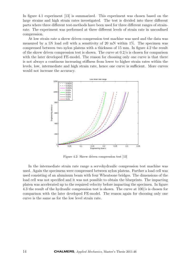
In figure 4.1 experiment [13] is summarized. This experiment was chosen based on thelarge strains and high strain rates investigated. The test is divided into three differentparts where three different test-methods have been used for three different ranges of strain-rate. The experiment was performed at three different levels of strain rate in unconfinedcompression.

At low strain rate a skrew driven compression test machine was used and the data wasmeasured by a 5N load cell with a sensitivity of 20 mN within 1%. The specimen wascompressed between two nylon platens with a thickness of 15 mm. In figure 4.2 the resultof the skrew driven compression test is shown. The curve at 0.2/s is chosen for comparisonwith the later developed FE-model. The reason for choosing only one curve is that thereis not always a continous increasing stiffness from lower to higher strain rates within thelevels, low, intermediate and high strain rate, hence one curve is sufficient. More curveswould not increase the accuracy.

0 0.05 0.1 0.15 0.2 0.25 0.3 0.350

200

400

600

800

1000

1200

Engineering strain ε

Eng

inee

ring

stre

ss σ

Low strain rate range

0.002/s0.002/s0.002/s0.02/s0.02/s0.02/s0.02/s0.2/s

Figure 4.2: Skrew driven compression test [13]

In the intermediate strain rate range a servohydraulic compression test machine wasused. Again the specimens were compressed between nylon platens. Further a load cell wasused consisting of an aluminum beam with four Wheatsone bridges. The dimensions of theload cell was not specified and it was not possible to obtain the blueprints. The impactingplaten was accelerated up to the required velocity before impacting the specimen. In figure4.3 the result of the hydraulic compression test is shown. The curve at 100/s is chosen forcomparison with the later developed FE-model. The reason again for choosing only onecurve is the same as for the low level strain rate.


0 0.05 0.1 0.15 0.2 0.25 0.3 0.35 0.40

500

1000

1500

2000

2500

3000

3500

4000

4500

5000


Eng

inee

ring

stre

ss σ

Intermediate strain rate range

20/s25/s90/s100/s160/s250/s260/s

Figure 4.3: Hydraulic compression test [13]

In the high strain rate region the method is changed to the split hopkinson pressure barmethod. The striker bar is impacted into the input bar creating an elastic wavefront. Thewavefront transmitts into the specimen and further into the output bar. An elastic wave isalso reflected at each boundary. These strains are then measured by the strain gauges andthen a calculation is performed yielding the stress strain response in the specimen [13]. Infigure 4.4 the result of the split hopkinson pressure bar is shown. These curves are shownfor completeness and this range of strain rate will not be modeled.

0 0.05 0.1 0.15 0.2 0.25 0.3 0.350

0.5

1

1.5

2

2.5

3

3.5x 10

6


Eng

inee

ring

stre

ss σ

High strain rate range

1800/s2100/s2100/s2700/s3500/s3600/s4400/s5700/s

Figure 4.4: Split hopkinson pressure bar [13]


4.1.2 Evaluation 1

Swift Indentation

Indentor

Plexiglas container

White adipose tissue

45 mm

d = 60 mm

d = 12 mm

Indentation velocity 2000 mm/s

4 mm

4 mm

t

Displacement profile

Depth

Figure 4.5: Swift indentation [8]

In the first evaluation experiment [8] in figure 4.5 a pneumatically driven piston of 12 mmdiameter is indented into a specimen of ovine WAT. The specimen is contained in a plasticcylinder. The force in the indentor is measured at a penetration depth of 4 mm. The resultfrom [8] can be seen in table 4.1. The value in the eighth cycle is used for later comparison.

Cycle 1 Cycle 2 Cycle 3 Cycle 4 Cycle 5 Cycle 6 Cycle 7 Cycle 8Mean Peak force (N) 13.3587 10.0279 9.8759 9.6057 9.6406 8.7956 8.9233 8.5679Standard deviation peak force (N) 6.1064 6.1330 5.7758 5.6079 5.8681 5.0864 5.2437 5.1378

Table 4.1: Peak force at 4 mm penetration. Mean value consists of 10 samples. Taken from [8]


4.1.3 Evaluation 2

Rotational Rheometer Constant Shear Strain

Range of Shear Strainrate 0.01/s - 1/s

d= 8 mm

h = 1.5 mm

Sandblasted Platen

Sandblasted Platen

Displacement Sequence

0.15

100s 100s

Specimen compressed with 1g force during

diplacement sequence

Shear Strain g

Time

Figure 4.6: Constant shear strain experiment [15]

The evaluation 2 experiment [15] is summarized in figure 4.6. The testing device used was arotational rheometer (Ares, Rheometric Scientific, USA) with sandblasted parallell plates.A slight compression of 1 gram was exerted on the specimen throughout the displacementsequence in order to increase the friction between the plates. Then a load and unloadingsequence was performed with a rest interval of 100 s between each load unloading cycle.The shear strain rate was increased with every cycle beginning at 0.01/s, proceeding with0.1/s and finally performed at 1/s.

−0.02 0 0.02 0.04 0.06 0.08 0.1 0.12 0.14 0.16−200

−100

0

100

200

300

400

500

shear strain γ

shea

r st

ress

τ [P

a]

Rotational rheometer

0.01/s0.1/s1/s

Figure 4.7: Constant shear strain experiment with increasing strain rate [15]


In figure 4.7 the result of the experiment is displayed. Only the loading part of thesecurves will be used for comparison according to the limitations of this thesis.

4.2 Mesh and Boundary Conditions

In this subsection the actual mathematical modelling of the three chosen experiments arepresented. Beginning, with modelling of the calibration experiment [13] in 4.2.1. Pro-ceeding, with modelling of evaluation 1 experiment [8] in 4.2.2. Finally, the modelling ofevaluation 2 experiment [15] in 4.2.3.

4.2.1 Modelling Calibration

x

z y

nylon platen shells

WAT hexahedral solid

Figure 4.8: Hexahedral mesh for the skrew driven unconfined compression test

The hexahedral mesh used to simulate the skrew driven compression test [13] is shownin figure 4.8. The upper nylon platen shell is displaced in the x-direction and the lowernylon plate shell is locked in all directions. The WAT hexahedral mesh rests on the contactformulations. An adequate mesh density of 600 hexahedrons have been established throughthe convergence study in appendix B. Allthough the convergence study was performed at100/s it is assumed that this mesh density is sufficient also for the test at strain rate0.2/s. The shells are covered with nullshells which are present in order to facilitate contactcalculations and does not contribute to the stiffness calculations. The friction betweenthe platens and the WAT has been modeled with a Coloumb friction formulation wherethe dynamic and static yield forces have been input. In order to determine reasonablevalues of the friction, a sensitivity analysis between compression force and friction hasbeen conducted in appendix E.


x

z y

nylon platen shells

WAT hexahedral solid

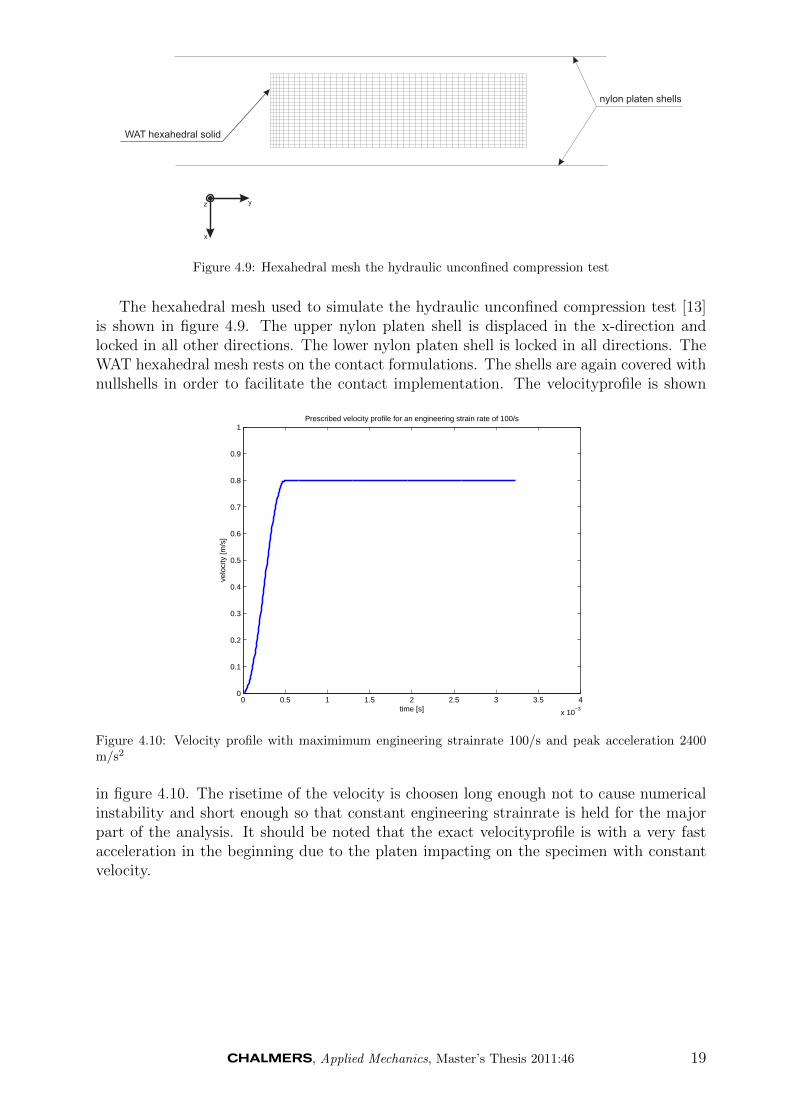
Figure 4.9: Hexahedral mesh the hydraulic unconfined compression test

The hexahedral mesh used to simulate the hydraulic unconfined compression test [13]is shown in figure 4.9. The upper nylon platen shell is displaced in the x-direction andlocked in all other directions. The lower nylon platen shell is locked in all directions. TheWAT hexahedral mesh rests on the contact formulations. The shells are again covered withnullshells in order to facilitate the contact implementation. The velocityprofile is shown

0 0.5 1 1.5 2 2.5 3 3.5 4

x 10−3

0

0.1

0.2

0.3

0.4

0.5

0.6

0.7

0.8

0.9

1

time [s]

velo

city

[m/s

]

Prescribed velocity profile for an engineering strain rate of 100/s

Figure 4.10: Velocity profile with maximimum engineering strainrate 100/s and peak acceleration 2400m/s2

in figure 4.10. The risetime of the velocity is choosen long enough not to cause numericalinstability and short enough so that constant engineering strainrate is held for the majorpart of the analysis. It should be noted that the exact velocityprofile is with a very fastacceleration in the beginning due to the platen impacting on the specimen with constantvelocity.


4.2.2 Modelling Evaluation 1

Indentor shell Container shellWAT hexahedral solid

x

yz

Figure 4.11: Hexahedral mesh of evaluation 1

The mesh used to simulate the evaluation 1 experiment [8] is shown in figure 4.11. Theindentor is placed half the shell thickness away from the WAT in order for it to be incontact from the beginning. The indentor shell is then accelerated upto a constant velocityof 2000 mm/s and then stopped at 4 mm penetration where the force is. The containeris represented by a shell. Note that there are small elements, not visible in figure, on theshells of the indentor and plastic cylinder which does not slow down the calculation sincethey are assigned ridgid material properties. The container shell is locked in all degrees offreedom and the WAT rests inside on the contact formulation between the shell and theWAT. The friction between the different parts is the coefficients established in appendixE. It is assumed that these coefficients would be the same as in the calibration.


4.2.3 Modelling Evaluation 2

x

z y

Lower boundary locked in all degrees of freedom simulating full friction

Upper boundary locked in x translational degree of freedom and subject to a rotation in

the yz-plane around x-direction according to the displacement profile

Figure 4.12: Hexa hedral mesh for simulation of rotational rheometer test, 200 hexahedrons

In figure 4.12 the mesh with a mesh density of 200 hexahedrons is shown used for thesimulation of evaluation 2 experiment [15]. The mesh density has been established througha convergence study in appendix B and this mesh density is assumed for all three levelsof strain rate. The friction has been assumed to be very high so as no slip occurs betweenthe platens and the specimen, this allows the model to be constructed without contactformulation. Further the compressive force present during the torsion of the specimen hasbeen assumed small enough to be neglected. It has been approximated to 20 Pa which isorder of magnitude lower than the shear stresses.

4.3 Simulations

Experiment Id Material model ν C1 C2 µ1 α1 K S1 T1 G1 β1 ρ G0

Calibration0.2/s CIH5O1 Ogden Rubber 0.499 - - 30 20 - - - 3000 310 920 -

CIH5Si1 Simp. Rubber 0.49 - - - - 5E5 - - - - 920 -CIH5So1 Soft Tissue - 100 100 - - 5E5 10 0.00322 - - 920 -

Calibration100/s CJH2O1 Ogden Rubber 0.4999983 - - 30 20 - - - 3000 310 920 -

CJH8Si1 Simp. Rubber 0.49 - - - - 5E8 - - - - 920 -CJH2So1 Soft Tissue - 100 100 - - 5E8 10 0.00322 - - 920 -

Evaluation 1E1OH2O1 Ogden Rubber 0.499 - - 30 20 - - - 3000 310 920 -E1OH2So1 Soft Tissue - 100 100 - - 5E5 10 0.00322 - - 920 -

Evaluation 21/s E2TH2O1 Ogden Rubber 0.499 - - 30 20 - - - 3000 310 920 -

E2TH2So1 Soft Tissue - 100 100 - - 5E5 10 0.00322 - - 920 -E2TH2T1 Viscoelastic - - - - - 2.296E6 1.169E5 100 - - 1200 3.506E5

Evaluation 20.1/s E2UH2O1 Ogden Rubber 0.499 - - 30 20 - - - 3000 310 920 -

E2UH2So1 Soft Tissue - 100 100 - - 5E5 10 0.00322 - - 920 -E2UH2T1 Viscoelastic - 100 100 - - 2.296E6 1.169E5 100 - - 1200 3.506E5

Evaluation 20.01/s E2VH2O1 Ogden Rubber 0.499 - - 30 20 - - - 3000 310 920 -

E2VH2So1 Soft Tissue - 100 100 - - 5E5 10 0.00322 - - 920 -E2VH2T1 Viscoelastic - 100 100 - - 2.296E6 1.169E5 100 - - 1200 3.506E5

Table 4.2: Table of material model parameters for simulations presented in the results section

In table 5.1 the simulations presented in the results section is shown. A detailed table ofsimulations is included in appendix G. Each simulation that is later presented in section 5is described below. All other simulations are presented in their respective appendix.


4.3.1 Calibration

The parameter values used in the simulation of the calibration experiment [13] are theparameters obtained after some adjustments, hence the values are the final values. Theparameters used for the Ogden Rubber model are µ1, which is the shear modulus, α1 whichis hardening parameter, G1 which is prony serie relaxation shear modulus and β1 which isrelaxation constant. Further a poisson’s ratio of ν = 0.499 is used for the low strain raterange and an implicit calculation is performed. For the intermediate strain rate range apoisson’s ratio of ν = 0.4999983 is used which corresponds, in small strain theory, to abulk modulus of 0.5 GPa. The density used is 920kg/m3.

−0.4 −0.3 −0.2 −0.1 0 0.1 0.2 0.3−5000

−4000

−3000

−2000

−1000

0

1000

2000

3000

4000

5000

engineering strain [dimensionless]

engi

neer

ing

stre

ss [P

a]

Input material curves for Simplified Rubber

Figure 4.13: Input material curves for Simplified Rubber

For the Simplified Rubber model a bulk modulus of K=5E5 has been used for the lowstrain rate range and K=5E8 for the intermediate strain rate range. The material inputcurves are presented in figure 4.13. The curves are not taken directly from the experimentin [13] but are created by using an expression for the uniaxial tension of the incompressibleOgden Rubber without viscoelastic contribution [23]. The reason for using two curves ateach range, two curves lies close to each other, is since if the strain rate is higher or lowerthan the one specified, the two curves closest to the actual rate will be used in the linearinterpolation. The density is set to 920kg/m3.

When calibrating the Soft Tissue model the parameters C1 and C2 are varied which arestiffness parameters. Further the prony serie is input by varying the coefficients S1 and T1which are the relaxation modulus and relaxation time respectively. The bulk modulus isset to K=5E5 for the low strain rate range and K=5E8 for the high strain rate range. Thedensity is set to 920kg/m3.

4.3.2 Evaluation 1

These simulations are performed for the Ogden Rubber material model and the Soft Tissuematerial model only. The Simplified Rubber material model is discarded due to convergenceproblems. The parameters calibrated in the previous section are used, shown in table 5.1.


4.3.3 Evaluation 2

These simulations are performed for the Ogden Rubber material model and the Soft Tissuematerial model only. The Simplified Rubber material model is discarded due to conver-gence problems. The parameters calibrated in the previous section are evaluated. Alsothe THUMS model, Viscoelastic 006 in LS-DYNA [21] is simulated for reference. Theparameters used are for the chest area of the THUMS HBM.

5 Results

The results section is divided into results from calibration [13], results from evaluation 1[8] and evaluation 2 [15].

5.1 Results from calibration

−0.05 0 0.05 0.1 0.15 0.2 0.25 0.3 0.35−200

0

200

400

600

800

1000

1200

1400

1600

σ [P

a] E

ngin

eerin

g st

ress

σ0/A

0

ε Engineering strain (L−L0)/L

0

Experiment 0.002/sExperiment 0.2/sCIH5O1 Ogden Rubber 0.2/sCIH5Si1 Simplified Rubber 0.2/sCIH5So1 Soft Tissue 0.2/s

Figure 5.1: Experimental curves taken from [13]

Material model ν C1 C2 µ1 α1 K S1 T1 G1 β1 ρOgden Rubber 0.499 - - 30 20 - - - 3000 310 920Simp. Rubber 0.49 - - - - 5E5 - - - - 920

Soft Tissue - 100 100 - - 5E5 10 0.00322 - - 920

Table 5.1: Table of material model parameters for low strain rate range

The experimental curves in figure 5.1 are taken from [13], from the low strain rate compres-sion test. The experimental curves are chosen with 0.2/s and 0.002/s strain rate. Thesestrain rates are the lowest and highest strain rates in the low strain rate region. The anal-yses are performed at a strain rate of 0.2/s. Note that the soft tissue material model isless nonlinear than the ogden model and the simplified rubber model.


−0.05 0 0.05 0.1 0.15 0.2 0.25 0.3 0.35 0.4−1000

0

1000

2000

3000

4000

5000

6000

7000

8000

9000

σ [P

a] E

ngin

eerin

g st

ress

σ0/A

0

ε Engineering strain (L−L0)/L

0

Experiment 160/sExperiment 25/sExperiment 100/sCJH2O1 Ogden Rubber 100/sCJH8Si1 Simplified Rubber 100/sCJH2So1 Soft Tissue 100/s

Figure 5.2: Experimental curves taken from [13]

The experimental curves in figure 5.2 are taken from [13], from the intermediate strain ratecompression test. The experimental curves are chosen with 100/s and 160/s strain rate.Note that the curve from the simplified rubber model is higher than the curves from theother models. Also note the peak in the beginning of the curves from the analyses andnote the abscence of this peak in the experiments.

Material model ν C1 C2 µ1 α1 K S1 T1 G1 β1 ρOgden Rubber 0.4999983 - - 30 20 - - - 3000 310 920Simp. Rubber 0.49 - - - - 5E8 - - - - 920

Soft Tissue - 100 100 - - 5E8 10 0.00322 - - 920

Table 5.2: Table of material model parameters for intermediate strain rate range


5.2 Results from evaluation 1

0 0.5 1 1.5 2 2.5

x 10−3

0

5

10

15

20

25

30

35Results of evaluation 1

E1OH2O1 Ogden RubberE1OH2So1 Soft Tissue

Figure 5.3: Ogden Rubber and Soft Tissue. Experimental curves taken from [8]

In figure 5.3 the results of evaluation 1 are presented. The Ogden Rubber and the SoftTissue model are presented. Note that the end values are around 2 N which is 25 percentof the experimental reported force at 4 mm penetration. The parameters in table 5.2.

5.3 Results from evaluation 2

−0.02 0 0.02 0.04 0.06 0.08 0.1 0.12 0.14 0.160

50

100

150

200

250

300

350

400

450Ogden Rubber

γ shear strain

τ sh

ear

stre

ss [P

a]

experiment 0.01/sexperiment 0.1/sexperiment 1/sE2TH2O1 Ogden Rubber 1/sE2UH2O1 Ogden Rubber 0.1/sE2VH2O1 Ogden Rubber 0.01/s

Figure 5.4: Ogden Rubber with linear viscoelasticity. Experimental curves taken from [15]


In figure 5.4 the ogden rubber model is compared to three different shear strain rates. Notethe difference in the slope. The experiment shows shear strain softening and the simulationshows shear strain hardening.

−0.02 0 0.02 0.04 0.06 0.08 0.1 0.12 0.14 0.160

50

100

150

200

250

300

350

400

450

γ shear strain

Soft Tissue

τ sh

ear

stre

ss [P

a]

experiment 0.01/sexperiment 0.1/sexperiment 1/sE2TH2So1 Soft Tissue 1/sE2UH2So1 Soft Tissue 0.1/sE2VH2So1 Soft Tissue 0.01/s

Figure 5.5: Soft Tissue with viscoelasticity. Experimental curves taken from [15]

In figure 5.5 the Soft Tissue model with viscoelasticity is simulated at three different shearstrain rates. Note the almost linear behaviour of the Soft Tissue model and the shearstrain softening of the experiment.

−0.02 0 0.02 0.04 0.06 0.08 0.1 0.12 0.14 0.160

0.5

1

1.5

2

2.5

3

3.5

4x 10

4

γ shear strain

THUMS linear viscoelastic

τ sh

ear

stre

ss [P

a]

experiment 0.01/sexperiment 0.1/sexperiment 1/sE2TH2T1 THUMS 1/sE2UH2T1 THUMS 0.1/sE2VH2T1 THUMS 0.01/s

Figure 5.6: Viscoelastic material model. Experimental curves, at bottom of figure, taken from [15]


In figure 5.6 the THUMS material model is simulated at three different strain rates. Notethe excess stiffness of the THUMS simulation. The experiments lies at the bottom of thegraph.

The parameters in table 5.1 are used for Ogden Rubber and Soft Tissue. The THUMSmaterial model parameters are ρ =1200 K=2.296E6 G0=3.506E5 Gi=1.169E5 β=100 .The Simplified Rubber input curves are from figure 4.13.

6 Discussion

The discussion section will begin with an analysis of the results of the simulation of the cal-ibration experiment. Proceeding with an analysis of the evaluation 1 experiment. Finally,a discussion of the result in the simulation of the experiment in evaluation 2.

6.1 Calibration

The Ogden rubber material model in figure 5.2 predicts the stress-strain behaviour in com-pression with excellent results. There is no need to make any improvements for the lowstrain rate region since the model is as good as the indata. The same applies to the Sim-plified Rubber material model 5.2. The soft tissue material model shows a weak nonlinearbehaviour. This is due to when the parameters of the model are tweaked according tosection 3.0.1 the model reduces to a Mooney Rivlin solid which is a special case of the twoterm Ogden Rubber with parameters α1 = 2 and α2 = −2. Since the Ogden Rubber modelin figure 5.2 has parameter α = 20 it is more nonlinear than the Mooney Rivlin which isof second order. The discrepancies between the Ogden Rubber model and the SimplifiedRubber model is just a matter of parameter tweaking, they have equal behaviour.

When predicting the intermediate strain rate region a value of 100/s was choosen. It canbe seen here also that the Soft Tissue model is less linear than the Ogden Rubber model,this difference is explained as previously. The peak in the beginning of the analysis comesfrom the inertial effects. Since the material is very compliant and the density rather higha small amount of acceleration gives a relatively large contribution to the overall forces.In the experiment there is no peak at the beginning. One possible explanation could bethat the density is set too high but this is rather unlikely since the same value has beenobserved in different papers. A more possible explanation or hint to where an explanationcould be found is in the test setup. It was not possible to obtain the blueprints of theloadcell and there might be something in its construction that filters these peaks.In theexperiment the platen was accelerated upto the choosen velocity and then impacted ontothe specimen. It was not possible to model this high acceleration, as in the impact, withthis high bulk modulus without getting an unstable solution. With a higher accelerationthe peak would become higher and thinner and could possibly be filtered away by the realtest setup, it might not even be registered by the measuring device. Since all three materialmodels has a peak in the beginning of the analysis it is less probable that the reason liesin the material modelling. The Soft Tissue is more similar to the Ogden rubber at thisstrain rate due to the fact that both has a viscoelastic contribution with a one term Pronyserie as relaxation function. The Simplified Rubber model deviates from the other twomodels since it has no hereditary integral that constitutes a fading memory effect of thestrain rate at previous timesteps. The Simplified Rubber has its stress-strain curve abovethe other material models and it is not possible to lower it any further at this strain rateand density. If the stiffness is reduced it asymptotically approaches a curve with the samepeak as with the original stiffness and the remaining curve is less nonlinear.


6.2 Evaluation 1

According to figure 5.3 and table 4.1 the simulation results for both material models areonly 25 percent of the experimental value in cycle 8. This could be due to several factors.For instance the indentor used in the experiment is flat ended and no radius is reported.Obviously it has to have a radius but how small it is is not documented. There hasn’t beenenough time in the project to make a study on the sensitivity of the force to the radiusand a radius of 1 mm have been used. It could be speculated at least that the force shouldincrease with decreasing radius but with what amount. The sensitivity might decrease withdecreasing radius but that is just a speculation. In order to decrease numerical instabilitythe indentor does not impact the specimen at full velocity rather accelerates from zeroupto 2000 mm/s in 0.1 ms. This is only 5 percent of the total simulation time. Due tothe relaxation time of 3.22 ms of the one term prony serie in both models this means thatit does not have time to fully relax. If a longer relaxation time had been set it could bespeculated that the force would be higher at 4mm penetration. Since the simulation time,due to the acceleration in the beginning, is a little bit longer than in reality the end valueof the simulation will be lower since the viscoelastic contribution would have relaxed to alower stiffness. This would result in a lower value of indentor force. It is quite riskful tocompare one value since there are oscillations in the force and they could be shifted slightlyin time due to different factors which would result in a value far away from the real valueeven though, if the whole experimental curve could have been obtained, it might have beenreally close in comparison. The opposite is also a risk. Further the ovine WAT might bestiffer than porcine or human WAT. In the experiment hexahedral elements were used witha 1 point integration solid element. Since they are subject to hourglassing, and hourglassformulation has been used. Unfortunately the hourglass forces are higher than the rule ofthumb, below 10 percent of peak internal energy. An hourglass sensitivity study has beenperformed which reveals little sensitivity between indentor force and hourglass coefficient,see appendix D.1.2. This might support the use of higher than 10 percent hourglass energy.

6.3 Evaluation 2

According to figure 5.4 the Ogden Rubber predicts the stresses with reasonable accuracybut it exhibits an opposite behaviour considering the stiffness. This is due to the factthat the experiment shows shear strain softening and the model is calibrated against acompression curve with strain hardening. If the model is calibrated with compressivestrain-hardening and tensile strain hardening it is unlikely that shear strain softening canfit in the model behaviour. Further the strain rate dependency is different in that themodel does not show as large increase with strain rate as the experiment. This is due tothe indata and can be accomodated by the model since more terms can be added to theprony series thus capturing a wider range of strain rates. In figure 5.4 looking at the curveof the Ogden rubber model at strain rate 1/s there is a small slope in the beginning withdecreasing stiffness. This is from the hereditary integral with one prony serie fitted tothe experiment in the calibration at 100/s. The small slope has similar behaviour as theexperiment curves but if this small slope would be expanded by use of shorter relaxationtimes the compressive behaviour would also be influenced since the same prony serie isused for all elements of the strain rate tensor, that is the same prony serie is used for allshear strains and strains in the hereditary integral according to section 3.0.3.

In figure 5.4 it can be seen that the Simplified Rubber model has a similar behaviouras the Ogden Rubber in figure 5.4. The difference is that there is no slope in the beginningof the curve at strain rate 1/s since there is no heriditary integrals involved, only linearinterpolation. This model cannot accomodate both tensile and compressive strain harden-


ing at the same time as shear strain softening since the input is a curve from a uniaxialtensile-compressive test. If shear strain softening is wished for the compressive and tensilestrain hardening would suffer. The strain rate dependency for this model is constant atthese ranges of strain due to the indata but the model can accomodate the strain ratestiffening response if the appropriate indata is input.

In figure 5.5 the results from the Soft Tissue material model is shown. This model ismore similar in its shear stress-strain response than the previous models but this modelcannot predict shear strain softening since it is linear in shear strain. The shear stressdepends on the Mooney Rivlin coefficients added and then multiplied by the shear strain,that is the two Mooney Rivlin coefficients added is equal to the shear modulus. The modelwith these particular parameters is does not represent the same amount of shear strainstiffening but it can be accomodated if fitted with indata from the correct strain raterange. The slope at the beginning of the curve at strain rate 1/s has the same explanationas for the Ogden Rubber model in figure 5.4

Figure 5.6 displays the THUMS model which is the LS-DYNA linear viscoelastic modelwith one term prony serie. The experiment curves have been flattened out and lies at thebottom of the figure since this model severely overestimates the stiffness and shear stressby a factor 102.


7 Conclusions

The Ogden Rubber would be suitable if range of strain rate is not too large otherwisethe Soft Tissue is a better choice while the Simplified Rubber is discarded due to severeconvergence problems. The Ogden Rubber would be the preferred choice if a stronglynonlinear behaviour in compressive-strain to compressive-stress is sought for. The SoftTissue would be more suitable if there are large shear strains that affect the human bodymodel. The Ogden Rubber would be preferred if incorrect shear strain representation andnarrow range of strain rate is weighed up by it being 6-7 times faster. Which model thatis the most preferred would be determined by future work and investigations.

8 Future Work

It is highly recommended to do further experiments on WAT due to paucity of availableexperiments and due to the small number of specimens and samples used in the up tonow conducted experiments. It is suggested tha porcine WAT be used since it is similarto human WAT. Especially, subcutaneous WAT at the porcine back middle layer which issimilar to deep subcutaneous WAT at the human abdomen [14]. Further, investigationsare needed on finding a similar depot site of the visceral human WAT, since this depot siteis relatively large in certain individuals.

Suggested experimental methods are unconfined compression, see work by [13]. Therehaven’t been conducted any experiments on the tensile behaviour of WAT, due to difficultiesin fastening of the specimen.

For evaluation an indentation experiment might be suitable since it produces a complexstrain field including all strain components such as, shear, compression and tension. For in-dentation experiments see work by [4]. If indentation is going to be used it is recommendednot to use a flat ended cylindrical indentor but rather one that has a radius at the end.This is to get rid of the sharp edge which is troublesome when modeling contact since itcomplicates contact modeling by introducing a lot of hourglassing due to the concentradedstress at the edge. A sharp edge does also require a higher mesh density in order for thesolution to converge, at least for convergence of the contact force.

Regarding the material models of this thesis, if one is going to be used it is recommendedto investigate the need to correctly represent the shear strains in an actual crash simulationsince both models underestimates the stiffness in shear for small values of strain andoverestimates for higher values of strain. Further a sensitivity analysis should be performedfor the wanted quantities with respect to the bulk modulus. This is since the bulk modulusof WAT is rather high which in turn slows down the explicit calculations considerably. Ifthe Ogden Rubber model is to be used, a sensitivity study of the wanted quantities withrespect to the poisson ratio is recommended since a very high poissons ratio, very close to0.5, indirectly increases the bulk modulus which in turn slows down explicit calculations.

References

[1] Saverio Cinti. The role of brown adipose tissue in human obesity. Nutrition,Metabolism & Cardiovascular Diseases, 16:569–574, 2006.

[2] Kerstyn Comley. A micromechanical model for the young’s modulus of adipose tissue.International Journal of Solids and Structures, 47:2982–2990, 2010.


[3] Livermore Software Technology Corporation. Ls-pre/post. http://www.lstc.com/

lspp, August 2011.

[4] Abbas Samani et al. A method to measure the hyperelastic parameters of exvivobreast tissue samples. Phys Med Biol, 49:4395–4405, 2004.

[5] Abbas Samani et al. Elastic moduli of normal and pathological human breast tissuesan inversion-technique-based investigation of 169 samples. Phys Med Biol, 52:1565–1576, 2007.

[6] Alison Sharpe Avram et al. Subcutaneous fat in normal and diseased states: 2.anatomy and physiology of white and brown adipose tissue. Journal of the AmericanAcademy of Dermatology, 53:671–683, 2005.

[7] A.M. Sims et al. Elastic and viscoelastic properties of porcine subdermal fat usingmri and inverse fea. Biomech Model Mechanobiol, 9:703–711, 2010.

[8] Amit Gefen et al. Viscoelastic properties of ovine adipose tissue covering the gluteusmuscles. Journal of Biomedical Engineering, 129:924–930, 2007.

[9] Dietrich Jehle MD et al. Influence of obesity on mortality of drivers in severe motorvehicle crashes. The american journal of emergency medicine, 234:34, 2010.

[10] D.J. Benson et al. A simplified approach for strain-rate dependent hyperelastic ma-terials with damage. Technical report, University of Californa, Dept. of Mechanicaland Aerospace Engineering, San Diego, USA; Daimler Chrysler AG, Sindelfingen,Germany; Consulting Engineer, Offenbach, Germany, 2006.

[11] Geerligs et al. Linear viscoelastic behaviour of subcutaneous adipose tissue. Biorhe-ology, 45:677–688, 2008.

[12] Javier Bonet et al. Nonlinear continuum mechanics for finite element analysis. Cam-bridge University Press, 2008.

[13] Kerstyn Comley et al. The mechanical response of porcine adipose tissue. ASMEJournal of Biomechanical Engineering, 2009.

[14] Klein et al. What are subcutaneous adipocytes really good for, viewpoint 5. Experi-mental Dermatology, 16:45–70, 2007.

[15] Marion Geerligs et al. Does subcutaneous adipose tissue behave asan(anti-)thixotropicmaterial? Journal of Biomechanics, 43:1153–1159, 2010.

[16] Martin AD et al. Adipose tissue density, estimated adipose lipid fraction and wholebody adiposity in male cadavers. International Journal of Obesity Related MetabolicDisorders, 18(2):79–83, 1994.

[17] Maurovich-Horvat et al. Comparison of anthropometric, area- and volumebased as-sessment of abdominal subcutaneous and visceral adipose tissue volumes using multi-detector computed tomography. International Journal of Obesity, 31:500–506, 2007.

[18] Noriyuki Ouchi et al. Adipokines in inflammation and metabolic disease. NatureReviews Immunology, 11:85–97, 2011.


http://www.lstc.com/lspp

http://www.lstc.com/lspp

[19] Parul Natvar Patel et al. Rheological and recovery properties of poly(ethyleneglycol)diacrylate hydrogels and human adipose tissue. Technical report, Department ofChemical Engineering, Rice University, Houston, Texas 77005 Laboratory of Repar-ative Biology and Bioengineering, Department of Plastic Surgery, The University ofTexas M.D., 2004.

[20] John O. Hallquist. LS-DYNA theory manual. LSTC, 2006.

[21] LSTC. LS-DYNA Keyword User’s Manual. LSTC, 2010.

[22] Kenneth Runesson. Constitutive Modeling of Engineering Materials - Theory andComputation. Chalmers University of Technology, 2006.

[23] Wikipedia. Ogden (hyperelastic model). http://en.wikipedia.org/wiki/Ogden_

(hyperelastic_model), Junet 2011.

[24] ZENBIO. Visceral preadipocytes and adipocytes. ZENBIO, 1:1, 2009.


http://en.wikipedia.org/wiki/Ogden_(hyperelastic_model)

http://en.wikipedia.org/wiki/Ogden_(hyperelastic_model)

A Finite Deformation Continuum Mechanics

A.1 Finite Deformation Kinematics

The motion of a body can be described by the mapping

x = Φ(X, t) (A.1)

This mapping is a transformation from the Lagrangian, material, formulation to theEularian, spatial, formulation. It is a transformation from the undeformed to the de-formed configuration. In order to transform quantities between the material and spatialconfiguration the deformation gradient is defined

F =∂Φ(X, t)

∂X(A.2)

In order to get a representation of the strain the right Cauchy-Green deformation tensoris defined as

C = FTF (A.3)

This can be interpreted as the transformation of the scalar product between two ele-mental vectors in the material configuration to the spatial configuration

dx1 · dx2 = dX1 ·CdX2 (A.4)

In order to calculate the difference between the scalar product of the elemental vectorsabove the Green strain tensor is introduced

E =1

2(C− I) (A.5)

This then becomes

1

2(dx1 · dx2 − dX1 · dX2) = dX1 · EdX2 (A.6)

The Green strain tensor is the equivalent of the small strain tensor in infinitesimalstrain theory since the infinitesimal strain tensor is obtained upon linearization of theGreen strain tensor

In order to pave the way for the viscoelastic contribution further on an expression forthe velocity is needed.

v(X, t) =∂φ(X, t)

∂t(A.7)

The above expression is differentiated with respect to the coordinates of the parti-cles in the body in the material configuration which produces the time derivative of thedeformation gradient

F =∂

∂X(∂φ

∂t) (A.8)

The material time derivative of the Green strain tensor is also needed.

E =1

2(FTF + FTF) (A.9)

To show how the above quantities are explicitly calculated an example of pure elongationwill be used


X1

X2

L

v

L

v

Ф

x1

x2

+vt/L

Figure A.1: Pure elongation

The displacement is the same as the above mentioned mapping

x = φ(X, t) (A.10)

The components of the displacement vector in this case becomes

x1 = X1 +X1vt/L (A.11)

x2 = X2 (A.12)

x3 = X3 (A.13)

where v is the velocity of the right edge in the material configuration, t is time and Lis the initial length.

F =∂x

∂X=

1 + vt/L 0 00 1 00 0 1

(A.14)

F =∂

∂X(∂φ

∂t) =

v/L 0 00 0 00 0 0

(A.15)


A.2 Stress Measures

The cauchy stress tensor is related to areas and forces in the current configuration, thedeformed configuration, in the following way.

dp = σda (A.16)

That is the common intuitive interpretation of stress. The second Piola-Kirchhoff stresstensor is instead a transformation of the cauchy stress into the initial configuration, theundeformed configuration. First, a pullback from the current to the initial configurationof the elemental force vector dp is performed.

dP = F−1dp (A.17)

Now equation (A.16) is inserted into equation (A.17) resulting in

dP = F−1σda (A.18)

The area elemental vector is still in the deformed configuration. Nanson’s formula isused in order to transform it into the undeformed configuration

dP = JF−1σFT︸︷︷︸S

dA (A.19)

A.3 Hyperelasticity

Hyperelasticity is defined as path independency of the material. That is the strain en-ergy function is only dependent on the initial and final state and not how that state wasreached[12]. This can be formulated as

Ψ(C(X),X) (A.20)

Ψ(IC , IIC , IIIC ,X) (A.21)

Ψ is the strain energy function. A definition of C can be found in appendix A.1. IC , IIC , IIICare the first, second and third invariant of a second order tensor and are equal to I : C,C : C and det(C) respectively. In (A.21) the strain energy is dependent not upon C butonly on its invariants which are invariant when the coordinate system is rotated. Since thisis isotropic hyperelasticity the strain energy is fully determined by the three invariants. Infor example transverse isotropy two additional invariants are needed in order to determinethe strain energy. Below is the expression for the second Piola Kirchhoff stress tensor foran isotropic material.

S = 2∂Ψ

∂C= 2

∂Ψ

∂IC

∂IC∂C

+ 2∂Ψ

∂IIC

∂IIC∂C

+ 2∂Ψ

∂IIIC

∂IIIC∂C

(A.22)

A.4 Hyperelasticity in Principal Directions

When looking at an isotropic hyperelastic material in the principal directions the strainenergy is a function of the principal stretches instead of the invariants of the right CauchyGreen strain tensor. In order to achieve this the square of the principal stretches and the


principal directions are obtained by calculating the eigenvalues and eigenvectors of C. Thisgives the expression for the second Piola Kirchhoff stress tensor as[12].

S =3∑

α=1

SααNα ⊗Nα; Sαα = 2∂Ψ

∂λ2α(A.23)

The above equation is the spectral representation of the second Piola Kirchhoff stress tensorwith the basevectors in the material configuration

A.5 Near incompressibility

When dealing with incompressible materials problems arise when used with the finite ele-ment method[12]. In order to get around this problem a nearly incompressible formulationis used instead where the strain energy is split into an isochoric and volumetric part asfollows.

Ψ(λ1, λ2, λ3) = Ψ(λ1, λ2, λ3) + U(J) (A.24)

The hat refers to isochoric deformation which is the deformation under constant volume.This implies that the determinant of the deformation gradient, the volume change, is equalto 1 and in the case of isotropy in principal directions this yields

λα = J1/3λα (A.25)

The term U(J) is the energy generated when the body experience volumetric defor-mation and since near incompressiblity is used as an approximation for incompressibility,U(J) needs to be accompanied by a penalty parameter that forces the body not to de-form volumetrically. That is it prohibits this way of deformation since due to the penaltyparameter a volumetric deformation would give a considerable contribution to the strainenergy as compared to isochoric deformation.


B Mesh Convergence

B.1 Calibration

In order to find out how many elements that are needed for the analyses a mesh convergencestudy is performed using successively larger mesh densities.

B.1.1 Hexahedral elements

The element used here is the default formulation in LS-DYNA, namely elform=1.

0 0.5 1 1.5 2 2.5 3 3.5

x 10−3

0

0.1

0.2

0.3

0.4

0.5

0.6

0.7Ogden rubber with viscoelastic contribution

time [s]

forc

e [N

]

CFH1O1 200 HexahedronsCFH2O1 600 HexahedronsCFH3O1 1200 Hexahedrons

Figure B.1: Mesh convergence with explicit calculation. Ogden model with viscoelastic contribution

According to figure B.1 it can be concluded that for the ogden model with viscoelasticcontribution it is sufficient with a mesh density with 600 hexahedrons for explicit calcula-tions.

0 0.5 1 1.5 2 2.5 3 3.5

x 10−3

0

0.2

0.4

0.6

0.8

1

1.2

1.4

time [s]

forc

e [N

]

Simplified rubber

CFH1Si1 200 HexahedronsCFH2Si1 600 HexahedronsCFH3Si1 1200 HexahedronsCFH7Si1 2000 HexahedronsCFH8Si1 3000 Hexahedrons

Figure B.2: Mesh convergence with explicit calculation.Simplified rubber with strain rate dependency


In figure B.2 it can be seen that the Simplified Rubber model requires around 2000hexahedral elements in order to reach convergence. This is around 3 times more than theOgden rubber model with viscoelastic contribution in figure B.1.

0 0.5 1 1.5 2 2.5 3 3.5

x 10−3

0

0.1

0.2

0.3

0.4

0.5

0.6

0.7

time [s]

forc

e [N

]

Soft tissue

CFH1So1 200 HexahedronsCFH2So1 600 Hexahedrons

Figure B.3: Mesh convergence with explicit calculation. Soft tissue with viscoelastic contribution

In figure B.3 it can be seen that the Soft tissue model with viscoelastic contributionreaches convergence with 600 hexahedral elements.

B.1.2 Tetrahedral elements

The element used here is a tetrahedral formulation in LS-DYNA, namely elform=13.

0 0.5 1 1.5 2 2.5 3 3.5

x 10−3

0

0.1

0.2

0.3

0.4

0.5

0.6

0.7Ogden rubber with viscoelastic contribution

time [s]

forc

e [N

]

5721 Tetrahedrons16444 Tetrahedrons82899 Tetrahedrons268984 Tetrahedrons


It can be seen in figure B.4 that there is sufficient convergence at 5721 tetrahedrons.


0 0.5 1 1.5 2 2.5 3 3.5

x 10−3

0

0.1

0.2

0.3

0.4

0.5

0.6

0.7

0.8

0.9

time [s]

forc

e [N

]

Simplified rubber

82899 Tetrahedrons268984 Tetrahedrons

Figure B.5: Mesh convergence with explicit calculation. Simplified rubber with strain rate dependency

According to figure B.5 the Simplified rubber model does not converge even at 268984tetrahedrons. No further increase in mesh density is necessary since the number of elementslargely exceeds the number required for convergence of the Ogden rubber and Soft tissuemodel.

0 0.5 1 1.5 2 2.5 3 3.5

x 10−3

0

0.1

0.2

0.3

0.4

0.5

0.6

0.7

time [s]

forc

e [N

]

Soft tissue

5721 Tetrahedrons82899 Tetrahedrons268984 Tetrahedrons

Figure B.6: Mesh convergence with explicit calculation.Soft tissue with viscoelastic contribution

It can be seen in figure B.6 that there is sufficient convergence at 5721 tetrahedrons.


B.2 Evaluation 1

0 0.5 1 1.5 2 2.5

x 10−3

0

2

4

6

8

10

12

14

16Ogden Rubber convergence test

E1OH1O1 215279 HexahedronsE1OH2O1 1434799 Hexahedrons


According to figure ?? it is reasonable to use a mesh density of 215279 hexahedrons forevaluation 2 with the Ogden Rubber material model.

0 0.5 1 1.5 2 2.5

x 10−3

0

10

20

30

40

50

60Soft Tissue convergence test

E1OH1So1 215279 HexahedronsE1OH2So1 1434799 Hexahedrons

Figure B.8: Mesh convergence with explicit calculation. Soft Tissue with viscoelastic contribution

According to figure B.8 it is reasonable to use a mesh density of 215279 hexahedronsfor evaluation 2 with the Soft Tissue material model.


B.3 Evaluation 2

0 0.05 0.1 0.15 0.2 0.25 0.3 0.35−500

0

500

1000

1500

2000

2500

3000

3500

4000

γ shear strain

τ sh

ear

stre

ss [P

a]

Convergence test Ogden Rubber

E2QH1O1 100 HexahedronsE2QH2O1 200 HexahedronsE2QH3O1 600 Hexahedrons

Figure B.9: Mesh convergence with implicit calculation. Ogden model with viscoelastic contribution

According to figure B.9 it can be concluded that for the ogden model with viscoelasticcontribution it is sufficient with a mesh density with 200 hexahedrons for implicit calcula-tions.

−0.02 0 0.02 0.04 0.06 0.08 0.1 0.12 0.14 0.160

50

100

150

200

250

γ shear strain

τ sh

ear

stre

ss [P

a]

Simplified Rubber convergence test

E2QH3Si1 600 HexahedronsE2QH4Si1 1200 HexahedronsE2QH5Si1 2100 Hexahedrons

Figure B.10: Mesh convergence with explicit calculation.Simplified Rubber with strain rate dependency

It can be seen in figure B.10 that convergence is not reached even at 2100 hexahedrons.This model is therefore discarded since it demands at lowest a factor of ten times morethan the Ogden Rubber to reach convergence.


0 0.02 0.04 0.06 0.08 0.1 0.12 0.14 0.160

50

100

150

200

250

300

350

400

γ shear strain

τ sh

ear

stre

ss [P

a]

Soft Tissue convergence test

E2QH2So1 200 HexahedronsE2QH3So1 600 Hexahedrons

Figure B.11: Mesh convergence with explicit calculation.Soft Tissue with viscoelastic contribution

As can be seen in figure B.11 a mesh of 200 hexahedrons is sufficient for convergence.

0 0.02 0.04 0.06 0.08 0.1 0.12 0.14 0.160

1

2

3

4

5

6

7

8x 10

4

γ shear strain

τ sh

ear

stre

ss [P

a]

THUMS convergence test

E2QH2T1 200 HexahedronsE2QH3T1 600 Hexahedrons

Figure B.12: Mesh convergence with explicit calculation.THUMS

According to figure B.12 it is considered safe to use a mesh density of 200 hexahedrons.


C Element formulation study

C.1 Element formulation Study

Since tetrahedral elements are going to be used in the future when meshing the WAT,an element formulation study has been performed comparing the converged hexahedralsolution with different element densities of the tetrahedral formulation.

C.1.1 Calibration

The hydraulic compression test has been used and the converged

0 0.5 1 1.5 2 2.5 3 3.5

x 10−3

0

0.1

0.2

0.3

0.4

0.5

0.6

0.7

time [s]

forc

e [N

]

Ogden rubber model with viscoelastic contribution

5721 Tetrahedrons600 Hexahedrons

Figure C.1: Ogden rubber model with viscoelastic contribution.

0 0.5 1 1.5 2 2.5 3 3.5

x 10−3

0

0.1

0.2

0.3

0.4

0.5

0.6

0.7

0.8

time [s]

forc

e [N

]

Simplified rubber model with strain rate dependency


Figure C.2: Simplified model with strain rate dependency.


0 0.5 1 1.5 2 2.5 3 3.5

x 10−3

0

0.1

0.2

0.3

0.4

0.5

0.6

0.7

time [s]

forc

e [N

]

Soft tissue


Figure C.3: Soft tissue model with viscoelastic contribution.

seconds/Tetrahedron at 5721 elements seconds/Tetrahedron at 268984 elementsOgden rubber 0.01 0.04Simplified rubber 0.03 0.13Soft tissue 0.07 0.23

Table C.1: Element processing as if run with 1 CPU.

speed factorOgden rubber - Simplified rubber 3Simplified rubber - Soft tissue 2Ogden rubber - Soft tissue 6-7

Table C.2: Table shows seconds/tetrahedron for the fastest material model, amongst the two compared,divided by seconds/tetrahedron for the slowest amongst the two compared.

The simulations has not been run with only one CPU hence their might be communi-cation between the CPU:s in the element processing time, but the speed factors in tableC.2 gives a hint of which ones the fastest, middle, and slowest.


D Hourglass formulation study

D.1 Hourglass formulation study

In order to find the appropriate hourglass formulation and hourglass coefficient a number ofdifferent formulations and coefficient have been tested at one strain rate with one materialmodel.

D.1.1 Calibration

In these tests the Ogden model is used with µ = 40, α = 20 and a viscoelastic contributionby a one term prony serie with coefficients β1 = 310 and G1 = 3000. The engineeringstrain rate is 100/s.

0 0.5 1 1.5 2 2.5 3 3.5

x 10−3

0

0.1

0.2

0.3

0.4

0.5

0.6

0.7

0.8

0.9

CMH2O9 Fully integrated element elform 3CMH2O12 IHQ 1 QM 0.05

0 0.5 1 1.5 2 2.5 3 3.5

x 10−3

0

0.1

0.2

0.3

0.4

0.5

0.6

0.7

0.8

0.9

CMH2O9 Fully integrated element elform 3CMH2O11 IHQ 1 QM 0.1

0 0.5 1 1.5 2 2.5 3 3.5

x 10−3

0

0.1

0.2

0.3

0.4

0.5

0.6

0.7

0.8

0.9

CMH2O11 IHQ 1 QM 0.1CMH2O12 IHQ 1 QM 0.05

0 0.5 1 1.5 2 2.5 3 3.5

x 10−3

0

1

x 10−4

CMH2O11 internal energy IHQ1 QM 0.1CMH2O11 Hourglass energy IHQ 1 QM 0.1

Figure D.1: Hourglass formulation study, mesh density 600 hexahedrons

According to figure D.1 a) it can be seen that the curve with 1 integration point elementis sufficiently similar to the fully integrated element. Further according to figure D.1 c)there is almost no difference between an hourglasscoefficient of 0.1 and 0.05 since the curvealmost overlaps. In figure D.1 d) it can be seen that the hourglass energy is very low incomparison with the internal energy and this formulation is used further on.


D.1.2 Evaluation Study 1

0 0.5 1 1.5 2 2.5

x 10−3

0

5

10

15

time [s]

forc

e [N

]

Ogden Rubber force sensitivity to hourglass coefficient

E1PH2O1 IHQ 1 QM 0.1E1PH2O2 IHQ 1 QM 0.005

Figure D.2: Hourglass formulation study

The hourglass coefficient have been varied from visible hourglassing modes in the simulationto no visible hourglassing modes. When there are no hourglass modes the hourglass energyis higher than the 10

0 0.5 1 1.5 2 2.5

x 10−3

0

10

20

30

40

50

60

time [s]

forc

e [N

]

Soft Tissue force sensitivity to hourglass coefficient

E1PH2So1 IHQ 1 QM 0.1E1PH2So2 IHQ 1 QM 0.001

Figure D.3: Hourglass formulation study

Acording to figure D.3 there is little influence of hourglass coefficient to the force inthe indentor with the Soft Tissue. It still does vary a bit in the end were the comparisonis going to be made but it is at least in the right ballpark.


E Frictional sensitivity analysis

The sensitivity of the forces with respect to the friction needs to be investigated in orderto see if frictional formulation is needed or not. If the force is very sensitive to the frictioncoefficients, care has to be taken in choosing the correct values.

E.1 Calibration

In these tests the Ogden model is used with µ = 40, α = 20 and a viscoelastic contributionby a one term prony serie with coefficients β1 = 310 and G1 = 3000. The engineeringstrain rate is 100/s. Further the dimensions of the specimen are radius 5 mm and length3 mm.

0 0.5 1 1.5 2 2.5 3 3.5

x 10−3

0

0.2

0.4

0.6

0.8

1

1.2

1.4

1.6

time [s]

forc

e [N

]

Force sensitivity with respect to friction

CHH2O1 zero frictionCHH2O2 FS 0.05 FD 0.04CHH2O3 FS 0.1 FD 0.09CHH2O4 FS 0.2 FD 0.19CHH2O5 FS 0.3 FD 0.29CHH3O6 FS 0.3 FD 0.29 1200 Hexahedrons

Figure E.1: Frictional sensitivity analysis. Ogden model with viscoelastic contribution

According to figure E.1 it can be concluded that for the ogden model with viscoelasticcontribution the friction has almost zero influence at small strains. At larger strains thecurves deviate and the force become more and more sensitive to friction with increasingvalues of the coefficients. According to Bjork steel on steel has friction coefficients FS=0.18and FD=0.14. It is reasonable to assume that WAT on nylon platens has lower values offriction coefficients. According to Bjork steel on steel with lubricated surfaces has frictioncoefficients FS=0.1 and FD =0.05. It is reasonable to assume that these values are veryclose to the values of WAT on nylon platens and since the sensitivity is lower when FS andFD are lower it becomes less critical to establish exact values on the friction coefficientshence FS=0.1 and FD=0.05 are going to be used further on for the WAT on nylon platens.In figure E.1 the black dashed line corresponds to an analysis with higher mesh densityand it can be concluded that the mesh density used is sufficient. This was done sincethe stressfield obviously changes as the friction coefficient is increased resulting in a morenonlinear stressfield.


F Stress sensitivity to bulk modulus or poissons ratio

In order to save analysis time it is reasonable to check the sensitivity of stress to the valueof the bulk modulus since a lowering of the bulk modulus reduces simulation time.

F.1 Evaluation 2

The simulation times for the three tests in evaluation 2 are relatively slow, 015 s, 1.5 s and15 s. The last two would take a considerable amount of time to calculate with the explicitmethod therefore the implicit method is used for all three. Further since the bulk modulusis relatively high the simulation time is also long for the implicit method. A sensitivitytest at 0.015 s simulation time with the explicit method has been performed with variouspoissons ratios and bulk modulus’ including the correct one, for all three material models.The calculations have been performed with elform=3 in order to eliminate hourglassing.The argument is since this sensitivity test is performed at a faster simulation time it wouldbe sufficient to validate the use of a lower poissons ratio or bulk modulus if there is lowenough sensitivity of poissons ratio or bulk modulus to the shear stress. This since thisfaster simulation will only increase inertial effects and stress due to strain rate dependencywhich would be a more severe case than the slower ones.

0 0.02 0.04 0.06 0.08 0.1 0.12 0.14 0.160

50

100

150

200

250

300

350

400

450

500

γ shear strain

τ sh

ear

stre

ss [P

a]

Ogden Rubber shear stress sensitivity to poisson‘s ratio

E2XH2O1 ν = 0.4999983E2XH2O2 ν = 0.499

Figure F.1: Mesh density 200 hexahedrons, elform = 3

As can be seen in figure F.1 it is assumed safe to use a poissons ratio of 0.499 for thethree tests in evaluation 2.


0 0.02 0.04 0.06 0.08 0.1 0.12 0.14 0.160

50

100

150

200

250

300

350

400

γ shear strain

τ sh

ear

stre

ss [P

a]

Soft Tissue shear stress sensitivity to bulk modulus

E2XH3So1 K = 5E5E2XH3So2 K = 5E8

Figure F.2: Mesh density 600 hexahedrons, elform = 1

As can be seen in figure F.2 it is assumed safe to use a bulk modulus between 5E5 to5E8 for the three tests in evaluation 2.


G List of simulations

Below follows a brief description of the various simulations performed on the Calibration,Evaluation 1 and Evaluation 2. A table of simulations is included in appendix amongstthe material keyword cards used in LS-DYNA.

Interpretation of simulation letter denominations

Simulation denomination, numbers also correspond to directory level of stored in- and output data

C_F_H1_O_1

1

1_2_3_4_5

2

3

4

5

Example of simulation denomination

1

2

3

4

5

H1: 215279 hexahedronsH2: 1434799 hexahedrons

O: Convergence testM: Hourglass sensitivity

E1: Evaluation

O: Ogden Rubber material modelSi: Simplified Rubber material modelSo: Soft Tissue material modelT: THUMS, Viscoelastic material model

1: Analysis nr. 12: Analysis nr. 23:...

1

2

3

4

5

H1: 100 hexahedronsH2: 200 hexahedronsH3: 600 hexahedronsH4:1200 hexahedronsH5:2100 hexahedrons

Q: Convergence testX: Bulk modulus sensitivityT: Model test at 1/sU: Model test at 0.1/sV: Model test at 0.01/s

E2: Evaluation



H1: 200 hexahedronsH2: 600 hexahedronsH3: 1200 hexahedronsH4: 1000 hexahedronsH5: 1800 hexahedronsH6: 2400 hexahedronsH7: 2000 hexahedronsH8: 3000 hexahedronsT1: 5721 tetrahedronsT2: 16444 tetrahedronsT3: 268984 tetrahedrons


F: Convergence test 100/sH: Variable friction test 100/sI: Model fit 0.2/sJ: Model fit 100/sM: Hourglass sensitivity

C: Calibration


Figure G.1: Simulation denominations and roadmap of directory structure for storing indata and outdata


Denomination Varied Parameters Value of varied parameter

Calibration

CFH1O1 Mesh density 200 elementsCFH2O1 Mesh density 600 elementsCFH3O1 Mesh density 1200 elementsCFH1Si1 Mesh density 200 elementsCFH2Si1 Mesh density 600 elementsCFH3Si1 Mesh density 1200 elementsCFH7Si1 Mesh density 2000 elementsCFH8Si1 Mesh density 3000 elementsCFH1So1 Mesh density 200 elementsCFH2So1 Mesh density 600 elementsCHH2O1 FS, FD FS 0 FD 0CHH2O2 FS, FD FS 0.05 FD 0.05CHH2O3 FS, FD FS 0.1 FD 0.1CHH2O4 FS, FD FS 0.3 FD 0.3CHH2O5 FS, FD FS 0.2 FD 0.2CHH3O6 FS, FD FS 0.3 FD 0.3CIH5O1 shear modulus µ1 α1 = 20, µ1 = 40, ρ = 920, G1 = 0, β1 = 0, ν = 0.4999983CIH5Si1 Input curves K = 0.5E9, SW = ST = SL = 1, TBID = 5000CIH5So1 C1, C2 XK = 0.5E9, S1 = 0, G1 = 0CJH2O1 shear modulus µ1, G1, β1 α1 = 20, µ1 = 30, ρ = 920, G1 = 3000, β1 = 310, ν = 0.4999983CJH8Si1 Input curves K = 0.5E9, SW = ST = SL = 1, TBID = 5000CJH2So1 C1, C2, S1, G1 XK = 0.5E9, S1 = 0.00322, G1 = 10CMH2O9 IHQ, QM, elform no hourglass formulation, elform=3CMH2O11 IHQ, QM, elform IHQ=1, QM=0.1, elform=1CMH2O12 IHQ, QM, elform IHQ=1, QM=0.05, elform=1

Table G.1: Table simulations for Calibration


Evaluation 1

E1OH1O1 Mesh density 215279 elementsE1OH2O1 Mesh density 1434799 elementsE1OH1So1 Mesh density 215279 elementsE1OH2So1 Mesh density 1434799 elementsE1PH1O1 IHQ, QM IHQ=1, QM=0.1E1PH1O2 IHQ, QM IHQ=1, QM=0.005E1PH1So1 IHQ, QM IHQ=1, QM=0.1E1PH1So2 IHQ, QM IHQ=1, QM=0.005

Table G.2: Table simulations for Evaluation 1



Evaluation 2

E2QH1O1 Mesh density 100 elementsE2QH2O1 Mesh density 200 elementsE2QH3O1 Mesh density 600 elementsE2QH3Si1 Mesh density 600 elementsE2QH4Si1 Mesh density 1200 elementsE2QH5Si1 Mesh density 2100 elementsE2QH2So1 Mesh density 200 elementsE2QH3So1 Mesh density 600 elementsE2QH2T1 Mesh density 200 elementsE2QH3T1 Mesh density 600 elementsE2XH2O1 ν ν = 0.4999983E2XH2O2 ν ν = 0.499E2XH3So1 K K=5E5E2XH3So2 K K=5E8E2TH2O1 none evaluation of already existing valuesE2TH2So1 none evaluation of already existing valuesE2TH2T1 none evaluation of already existing valuesE2UH2O1 none evaluation of already existing valuesE2UH2So1 none evaluation of already existing valuesE2UH2T1 none evaluation of already existing valuesE2VH2O1 none evaluation of already existing valuesE2VH2So1 none evaluation of already existing valuesE2VH2T1 none evaluation of already existing values

Table G.3: Table simulations for Evaluation 2


H Material Keycards

The material keyword cards are presented for the material models used in the simulations.The keyword cards are presented with the final parameter values after the calibration ex-periment. The Simplified Rubber model has TBID 5000 as input curves which correspondsto the curves in figure 4.13.

*MAT_OGDEN_RUBBER

$# mid ro pr n nv g sigf

2 920 0.4999983 0 6 0.000 0.000

$# mu1 mu2 mu3 mu4 mu5 mu6 mu7 mu8

30 0.000 0.000 0.000 0.000 0.000 0.000 0.000

$# alpha1 alpha2 alpha3 alpha4 alpha5 alpha6 alpha7 alpha8

20.000000 0.000 0.000 0.000 0.000 0.000 0.000 0.000

$# Gi Bi

3E3 310

*MAT_SOFT_TISSUE_VISCO_TITLE

softtissue

$# mid ro c1 c2 c3 c4 c5

1 920.00000 100 100 0.000 0.000 0.000

$# xk xlam fang xlam0

5.0000E+8 10.000000 0.000 0.000

$# aopt ax ay az bx by bz

2.000000 0.000 1.000000 0.000 0.000 0.000 1.000000

$# la1 la2 la3 macf

0.000 0.000 0.000 1

$# s1 s2 s3 s4 s5 s6

10 0.000 0.000 0.000 0.000 0.000

$# t1 t2 t3 t4 t5 t6

0.00322 0.000 0.000 0.000 0.000 0.000

*MAT_SIMPLIFIED_RUBBER/FOAM_TITLE

simplified

$# mid ro k mu g sigf ref prten

3 920.00000 5.0000E+8 0.000 0.000 0.000 0.000 0.000

$# sgl sw st lc/tbid tension rtype avgopt pr/beta

1.000000 1.000000 1.000000 5000 1.000000 1.000000 0.000 0.000

*MAT_VISCOELASTIC

$# mid ro bulk g0 gi beta

4 1200 2.2960E+6 3.5060E+5 1.1690E+5 100.00000

Figure H.1: Material keyword cards used in LS DYNA [21]


evaluation of material models in ls-dyna for impact...

Documents