evaluation of intelligent intrusion detection models · evaluation of intelligent intrusion...

International Journal of Digital Evidence Summer 2004, Volume 3, Issue 1

Evaluation of Intelligent Intrusion Detection Models

Nasser S. Abouzakhar Gordon A. Manson

University of Sheffield

Abstract This paper discusses an evaluation methodology that can be used to assess the performance of intelligent techniques at detecting, as well as predicting, unauthorised activities in networks. The effectiveness and the performance of any developed intrusion detection model will be determined by means of evaluation and validation. The evaluation and the learning prediction performance for this task will be discussed, together with a description of validation procedures. The performance of developed detection models that incorporate intelligent elements can be evaluated using well known standard methods, such as matrix confusion, ROC curves and Lift charts. In this paper these methods, as well as other useful evaluation approaches, are discussed. Introduction Evaluation is the key in making significant progress in applying intelligent solutions and machine learning algorithms to real life problems, such as intrusion detection [Witten et. al. 2000]. However, systematic ways to evaluate how different learning methods work and to compare one with another are needed, as well as ways of predicting performance based on practical experiments using useful collected data. Evaluating the performance of machine learning schemes on a given problem, such as detecting and predicting unauthorised activities within a network, is an issue that is not easy as it sounds. So far, experiments have been conducted and it has been assumed that what is being predicted is the ability to classify different instances of normal and abnormal network traffic activities. In some other experimental situations, the prediction involves class probabilities, rather than only the classes themselves. For example, a developed model predicted a smurf activity and indicated that it was in a form of a probabilistic figure based on the behaviour of ICMP protocol. Therefore, a mechanism for maximising the success rate of the predictions and counting the cost of making wrong decisions and predictions is needed. In most practical intrusion detection situations, the cost of a misdetection error depends on the type of error it is, e.g. whether a positive signal was erroneously detected as negative or vice versa. When developing an intelligent-based solution such as an intrusion detection model, and evaluating its performance, it is often essential to take these costs into consideration.

www.ijde.org


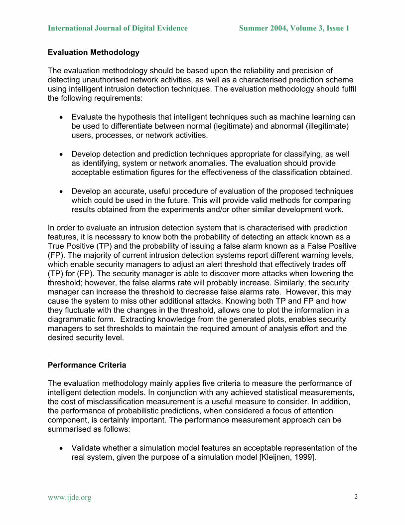
Evaluation Methodology The evaluation methodology should be based upon the reliability and precision of detecting unauthorised network activities, as well as a characterised prediction scheme using intelligent intrusion detection techniques. The evaluation methodology should fulfil the following requirements:

• Evaluate the hypothesis that intelligent techniques such as machine learning can be used to differentiate between normal (legitimate) and abnormal (illegitimate) users, processes, or network activities.

• Develop detection and prediction techniques appropriate for classifying, as well

as identifying, system or network anomalies. The evaluation should provide acceptable estimation figures for the effectiveness of the classification obtained.

• Develop an accurate, useful procedure of evaluation of the proposed techniques

which could be used in the future. This will provide valid methods for comparing results obtained from the experiments and/or other similar development work.

In order to evaluate an intrusion detection system that is characterised with prediction features, it is necessary to know both the probability of detecting an attack known as a True Positive (TP) and the probability of issuing a false alarm known as a False Positive (FP). The majority of current intrusion detection systems report different warning levels, which enable security managers to adjust an alert threshold that effectively trades off (TP) for (FP). The security manager is able to discover more attacks when lowering the threshold; however, the false alarms rate will probably increase. Similarly, the security manager can increase the threshold to decrease false alarms rate. However, this may cause the system to miss other additional attacks. Knowing both TP and FP and how they fluctuate with the changes in the threshold, allows one to plot the information in a diagrammatic form. Extracting knowledge from the generated plots, enables security managers to set thresholds to maintain the required amount of analysis effort and the desired security level. Performance Criteria The evaluation methodology mainly applies five criteria to measure the performance of intelligent detection models. In conjunction with any achieved statistical measurements, the cost of misclassification measurement is a useful measure to consider. In addition, the performance of probabilistic predictions, when considered a focus of attention component, is certainly important. The performance measurement approach can be summarised as follows:

• Validate whether a simulation model features an acceptable representation of the real system, given the purpose of a simulation model [Kleijnen, 1999].

www.ijde.org 2


• Evaluate the precision of the developed detector model using a confusion matrix [Witten et. al., 2000].

• Evaluate the performance of a developed detector model on an unseen test set

using 10-fold stratified cross-validation [Witten et. al., 2000]. This can be applied when a dataset is used to train a developing model.

• Measure the performance of a model and its cost of misclassification using Lift

charts and ROC curves [Marchette, 2001]. The effectiveness of these measures can be summarised and tested for statistical significance of a particular developed model. For example, intelligent simulation tools that model intrusion detection should enable the use of several different evaluation features to conduct evaluation experiments and measurements. The primary goal of developing intelligent detection models, which function as prediction and classification mechanisms, is to predict the performance of a detector on new events and assess its error rate on unseen data (i.e. a dataset that played no part in the formation or training of the detector model under development). The ultimate goal in the detection task is to identify those potentially unauthorised activities and malicious occurrences in user processes or networks, while minimising the rate of incorrectly flagging normal behaviours, i.e. false positives. This is to minimise the rate of failing to identify unauthorised activities and malicious behaviours, i.e. false negatives. The false positives and false negatives rate of an entire detection system must be as low as possible. Even though it is possible to bundle the testing data back into the training data, the testing data used to test the developed detection model has to be kept separate from the training data. The reason for that is the amount of training data that is used to develop the detector model is often huge. In fact what is important is that error rates are quoted based on the separation of both training data and testing data. This matches the assumption made by Witten et. al. [2000] that both the training data and the test data are representative samples of the underlying problem. Provided both samples are representative, the error rate on the test set will give a true indication of future performance. The larger the training sample, the better the detection classification, although the returns begin to diminish once a certain volume of training data is exceeded. And, the larger the test sample, the more accurate the error estimate. However, it is possible to increase the level of confidence significantly through careful examination of the dataset, as well as related experiments. The accuracy of the error estimate can be quantified statistically. One of the dataset that is often used in the development and evaluation of intrusion detection models is generated by MIT Lincoln Lab [MIT Lincoln Lab], which was mostly recently updated in 2000. This dataset contains millions of instances in a form of network connections using different networks as well as application protocols. The learning procedures for developing network detector models can only receive the dataset as an input. In order to increase the efficiency of such experiments,

www.ijde.org 3


accommodate a huge dataset, and achieve accurate modelling and simulation results, high specification hardware is required. In such a developed detection model, the techniques used for the development can be easily compared, because all of them received the same training dataset as input. Therefore, it is possible to quantify the effect of the local structures on the parameter estimation and the structure selection of those developed detection models. Validation of Modelling & Training Dataset Validation determines whether a simulation model is an acceptable representation of a real system given the purpose of a simulation model [Kleijnen, 1999]. In this case simulation means experimentation, i.e., the model is used instead of the real system. Also, real data are used rather than simulated data; hence, experimentation is done using a simulated model rather than the real system. However, any experimentation calls for statistical analysis, which is only part of the whole validation process. The type of statistical procedure to use depends on the kind of data that is available for the analysis. When a model is created such as a detection model, it should be developed for a well defined purpose, and its validity and performance determined with respect to that purpose [Sargent, 1999]. If the purpose of a model is to answer particular questions, the validity of the model has to be determined with respect to each question. There are many validation techniques that can be used to validate a particular intrusion detection model. In Sargent [1999], sixteen various general validation techniques were discussed. These techniques were used for general purposes. However, only eight of them are applicable here to validate intrusion detection models that feature intelligent solutions. In addition combinations of the eight selected techniques can be used, which is quite acceptable within the verification and validation (V&V) community. The other validation techniques are excluded due to their irrelevance to the underlying problem. Following Sargent [1999], the selected validation techniques that can be used to validate simulated intrusion detection models are as follows.

• Parameter Variability-Sensitivity Analysis: This technique consists of altering the values of the internal parameters of a developed model and its inputs to determine the effects upon the model’s behaviour and its output. The same relationships of change should be possible in the real system model.

• Predictive Validation: The model is used to predict the system behaviour;

consequently, comparisons can be made between the model’s prediction and the system’s behaviour to determine if they are similar. The empirical evidence could be used here to make the comparisons.

• Operational Graphics: This is used to obtain various performance measures that

graphically indicate the model behaviour with respect to time, i.e., the dynamic behaviours of performance indicators are visually displayed as the simulation model moves through time.

www.ijde.org 4


• Historical Data Validation: If historical data is available (or if data is collected on a system for building or testing the model), part of the historical data is used to train; hence, building the model and the remaining unseen part is used to test whether the model behaves in a similar manner to the real system.

• Historical Methods: The three historical methods of validation are rationalism,

empiricism, and positive economics. Rationalism assumes that everyone knows whether the underlying assumptions of a model are true. Logic deductions are used from these assumptions to develop the correct model. Empiricism requires every assumption, achieved model output and outcome to be empirically validated. Positive economics requires only that the model be able to predict the future and is not concerned with a model’s assumptions or structure (causal relationship or mechanism).

• Multistage Validation: proposed by Naylor and Finger, [1967], this technique

combines the three historical methods of rationalism, empiricism, and positive economics into a multistage process of validation. This validation method consists of, first developing the model’s assumptions on theory, observations, general knowledge, and function, second validating the model’s assumptions where possible by empirically testing them, and finally, comparing the input-output relationships of the developed model to the real system.

• Traces: The idea behind this technique is to trace the behaviour of different types

of specific entities in the model. This is to determine if the model’s logic is correct and if the necessary accuracy is achieved.

• Turing Tests: This validation test is based on the consultation of experts who are

familiar with the underlying problem and knowledgeable about the operations of a system. They can be asked identify any differences between the developed model and a real system outputs.

It is natural to measure a detector’s prediction performance in terms of the error rate [Witten et. al., 2000]. If the prediction is correct, then it is counted as a success; otherwise it is an error. Generally, in order to predict the performance of a detector on new input data, such as new incoming network traffic, its error rate must be assessed on an independent dataset that played no part in the formulation of the detector. There are two datasets that should be provided, the training data and the test data. The training data will be used to come up with the detector. Then the test data will be used to calculate the error rate of the final, optimised model. Each of the two sets must be chosen independently. The testing data set must be different from training data to get a reliable estimate of the true error rate and to get good performance in the optimisation or evaluation stage. The validation process will then be used to optimise the internal parameters of developed detector models, so to evaluate which approach would be more suitable. Provided all samples are representative, the error rate on the test set will give a true indication of future performance.

www.ijde.org 5


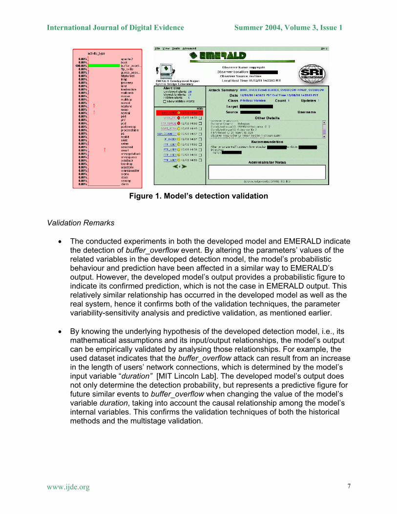
Generally, there is no straight forward way to tell whether a sample is representative or not. One possible way of evaluating the Bayesian Learning approach is to determine the error rate using stratified tenfold cross-validation. Stratification is a technique which ensures that random sampling is done in such a way as to guarantee that each class is properly represented in both training and test sets [Witten et. al., 2000]. The standard way of predicting the error rate estimate of a learning technique given a single, fixed sample of data is to use stratified tenfold cross-validation. This technique is used in such away that the dataset is divided randomly into ten parts, in each of which the class is represented in approximately the same proportions as in the full dataset. Each part is held out in turn and the learning scheme trained on the remaining nine-tenths; then its error rate is calculated on the holdout set. Thus the learning procedure is executed a total of ten times, on different training sets (each of which have a lot in common). Finally, the ten error estimates are averaged to yield an overall error estimate. The stratified tenfold cross-validation is considered to be a standard evaluation technique in practical terms. Due to the possible substantial variance in an individual tenfold cross-validation and the approximation of the true cross-validation error figure, it is possible to sample from the distribution of cross-validation experiments. This can be achieved by using different random partitions of a given dataset, treating error rates calculated in these cross-validation runs as different, independent samples from a probability distribution. Therefore, by comparing the average error rate over several cross-validations for a learning model, it is possible to determine whether a mean of a set of samples of a cross-validation estimate is significantly greater or significantly less. Validation of Model’s Detection: A case study An intrusion detection model that is developed using a Bayesian network learning has been validated by comparing its output with a real system, EMERALD (Event Monitoring Enabling Responses to Live Disturbances) detection system’s output. The developed detector model has been automatically learned and trained from the MIT Lincoln Lab dataset. EMERALD is SRI’s environment for scalable, distributed intrusion detection and network monitoring [Marchette, 2001]. (Information on EMERALD can be obtained from many recent sources on intrusion detection [Amoroso, 1999, Bace, 2000, Marchette, 2001]). Figure 1 indicates that both the developed model output and EMERALD system are detecting buffer_overflow activities [Valdes et al, 2001]. In order to protect the data, part of the information on EMERALD’s output is hidden. A similar relationship of the developed model change appears in the real EMERALD system as a result of internal parameters changes. However, the developed model’s output provides a probabilistic figure to indicate its confirmed prediction.

www.ijde.org 6


Figure 1. Model’s detection validation

Validation Remarks

• The conducted experiments in both the developed model and EMERALD indicate the detection of buffer_overflow event. By altering the parameters’ values of the related variables in the developed detection model, the model’s probabilistic behaviour and prediction have been affected in a similar way to EMERALD’s output. However, the developed model’s output provides a probabilistic figure to indicate its confirmed prediction, which is not the case in EMERALD output. This relatively similar relationship has occurred in the developed model as well as the real system, hence it confirms both of the validation techniques, the parameter variability-sensitivity analysis and predictive validation, as mentioned earlier.

• By knowing the underlying hypothesis of the developed detection model, i.e., its

mathematical assumptions and its input/output relationships, the model’s output can be empirically validated by analysing those relationships. For example, the used dataset indicates that the buffer_overflow attack can result from an increase in the length of users’ network connections, which is determined by the model’s input variable “duration” [MIT Lincoln Lab]. The developed model’s output does not only determine the detection probability, but represents a predictive figure for future similar events to buffer_overflow when changing the value of the model’s variable duration, taking into account the causal relationship among the model’s internal variables. This confirms the validation techniques of both the historical methods and the multistage validation.

www.ijde.org 7


Intelligence Evaluation and Analysis Intelligence means the capability of a detection model to automatically learn and predict the relationship among its internal variables. In this section, a targeted evaluation will be used to measure the quality of a detector model for the prediction of the target variable and its parameters with respect to an associated dataset. Once the detection model is learned, it is possible to evaluate its performance on a test set (ideally different from the training learning set). The tools that can be used for evaluating detection model are as follows [Marchette, 2001, BayesiaLab, 2003]:

• Confusion Matrices allow the precise measurement of the performance of a model for each modality (events occurrence number, reliability -- proportion of the cases with a correct prediction, and precision -- proportion of the cases where the true value is correctly predicted);

• ROC curves, which are centred on the parameter value of the target node

(activity_type), and ;

• Lift charts, which are centred on the parameter value of the target node as well. The following sections will focus on the use of a confusion matrix, ROC curves and Lift charts to evaluate network detector models. Confusion Matrix The effectiveness of a learning classifier is its ability to make correct classification decisions. There are several evaluation measures used for measuring effectiveness including reliability and precision. Classification could be thought of as a number of binary decisions where each entry in an assignment table is given a {0, 1} score (a binary yes/on decision) [Witten et. al., 2000]. One parameter that is used for evaluation is the cost of making wrong decisions and wrong classifications. Optimising classification rate without considering the cost of the errors often leads to inaccurate results. In networks security terms the cost of incorrectly detecting abnormal network behaviour classification has a different cost to the incorrectly predicted normal classification outcome. In networks intrusion detection, the primary concern is a two-class case attack “yes” or attack “no”. The four different possible outcomes of a single prediction are shown in Table 1, which is known as the confusion matrix for the two-class case. The true positives (TPs) and true negatives (TNs) are correct classifications. The false positive (FP) is when the outcome is incorrectly predicted as yes (or positive), when it is in fact no (negative). A false negative (FN) is when the outcome is incorrectly predicted as negative, when it is in fact positive. These two kinds of errors will generally have different costs; likewise the two types of correct classification will have different benefits.

www.ijde.org 8


Table 1. Different outcomes of a two-class prediction

True or real class(or values)

Predicted class(or values) Yes No

Yes True Positive (TP) False Negative (FN)

No False Positive (FP) True Negative (TN)

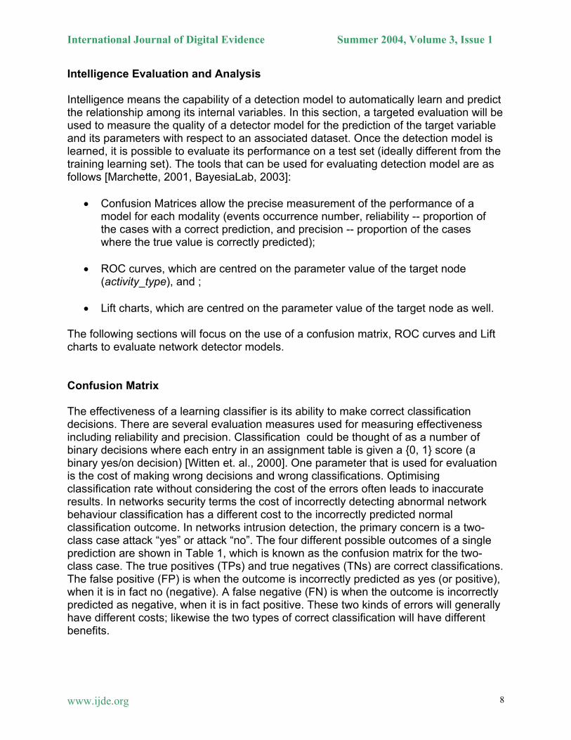
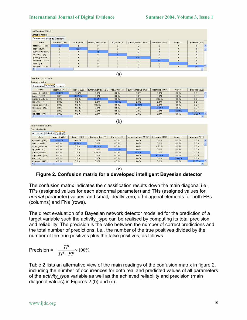
The confusion matrices that are shown in Figures 2 (a), (b), and (c) were produced for a developed intelligent detector model incorporated with Bayesian learning. These figures give useful feedback about its performance. This detector has been developed and automatically learned using the MIT Lincoln Lab dataset. Three visualization modes are available, as follows:

• Occurrence Matrix: number of cases for each Prediction/Real value, as shown in Figure 2 (a). The predictions of the model appear on the columns, the lines are representing the true (real) values that are in the dataset.

• Reliability Matrix: ratio between each prediction and the total number of the

corresponding prediction (sum of the line) , as shown in Figure 2 (b).

• Precision Matrix: ratio between each prediction and the total number of the corresponding real value (sum of the column), as shown in Figure 2 (c).

www.ijde.org 9


(a)

(b)

(c)

Figure 2. Confusion matrix for a developed intelligent Bayesian detector The confusion matrix indicates the classification results down the main diagonal i.e., TPs (assigned values for each abnormal parameter) and TNs (assigned values for normal parameter) values, and small, ideally zero, off-diagonal elements for both FPs (columns) and FNs (rows). The direct evaluation of a Bayesian network detector modelled for the prediction of a target variable such the activity_type can be realised by computing its total precision and reliability. The precision is the ratio between the number of correct predictions and the total number of predictions, i.e., the number of the true positives divided by the number of the true positives plus the false positives, as follows

Precision = 100%TPTP FP

×+

Table 2 lists an alternative view of the main readings of the confusion matrix in figure 2, including the number of occurrences for both real and predicted values of all parameters of the activity_type variable as well as the achieved reliability and precision (main diagonal values) in Figures 2 (b) and (c).

www.ijde.org 10


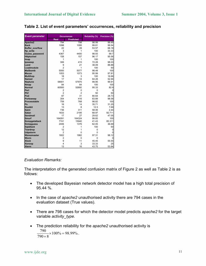
Table 2. List of event parameters’ occurrences, reliability and precision Event parameter Occurrences Reliability (%) Precision (%)

Real PredictedApache2 794 798 98.99 99.49Back 1098 1095 99.81 99.54Buffer_overflow 22 28 53.57 68.18ftp_write 3 1 100 33.33Guess_password 4367 4400 98.93 99.7Httptunnel 158 157 96.17 95.56Imap 1 1 100 100Ipsweep 306 415 72.28 98.03Land 9 21 38.09 88.88Loadmodule 2 1 100Mailbomb 5000 5077 98.48 100Mscan 1053 1073 95.99 97.81Multihop 18 3 100 16.66Named 17 14 64.28 52.94Neptune 58001 57975 99.95 99.91Nmap 84 84 100 100Normal 60593 52692 95.33 82.9Perl 2 0 0Phf 2 2 50 50Pod 87 31 80.64 28.73Portsweep 354 416 83.89 98.58Processtable 759 768 98.82 100Ps 16 14 35.71 31.25Rootkit 13 8 12.5 7.69Saint 736 311 58.06 2.44Satan 1633 2195 68.97 92.711Sendmail 17 27 29.62 47.05Smurf 164091 164324 99.85 100Snmpgetattack 7741 15940 41.43 85.311Snmpguess 2406 1376 62.05 36.69Sqlattack 2 1 100Teardrop 12 1 0 0Udpstorm 2 0 0Warezmaste

50

0

50

0r 1602 1982 97.31 98.12

Worm 2 0 0Xlock 9 11 45.45 55.55Xsnoop 4 3 33.33 25Xterm 13 16 43.75 53.84

0

Evaluation Remarks: The interpretation of the generated confusion matrix of Figure 2 as well as Table 2 is as follows:

• The developed Bayesian network detector model has a high total precision of 95.44 %.

• In the case of apache2 unauthorised activity there are 794 cases in the

evaluation dataset (True values).

• There are 798 cases for which the detector model predicts apache2 for the target variable activity_type.

• The prediction reliability for the apache2 unauthorised activity is

790 100% 98.99%790 8

× =+

.

www.ijde.org 11


• The prediction precision for the apache2 unauthorised activity is 790 100% 99.49%

790 4× =

+.

• Due to the low representation of buffer_overflow in the training dataset, the

achieved prediction reliability is 53.57% and the prediction precision is 68.18%.

• For those unpredicted parameters, i.e., with zero or nearly zero prediction, such as Udpstorm or Teardrop, the achieved reliability and precision is zero. This is due to the inappropriate representation of those parameters.

• Good classification results correspond to large numbers down the true main

diagonal on the confusion matrix and small, ideally zero, off-diagonal elements. The ROC Curves and Lift charts One of the methods that is used for counting the cost and evaluating machine learning schemes is known as ROC (Receiver Operating Characteristics) curves, where the learner is trying to select samples of test instances that have a high proportion of positives [Witten et. al., 2000]. ROC] is a procedure derived from the early days of radar and sonar detection used in the Second World War, hence the name “Receiver Operating Characteristic” [O’Connell et. al., 2002 . ROC is used in signal detection to characterise the trade off between hit rate and false alarm rate over a noisy channel. The features supplied with ROC can be used to evaluate the performance of intrusion detection models that incorporate intelligent solutions. The ROC curve plots the number of positives included in the sample on the vertical axis (Y-axis), expressed as a percentage of the total number of positives or the true positive rate, against the number of false positives included in the sample, expressed as a percentage of the total number of false positives or the false positive rate, on the horizontal axis (X-axis). Another common graphical method used to evaluate and validate the machine learning solutions, and therefore used to evaluate intelligent detection models, is known as Lift chart technique. Lift charts are closely related to the ROC graphical technique as an evaluation measure. They are used in just the same situation as above, where the learner is trying to select samples of test instances that have a high proportion of positives. The lift chart represents the detection rate of the target variable value (Vertical axis) proportional to the number of processed cases (Horizontal axis) based on the order defined by the learned model. The Y-axis represents the number of responses obtained, and the X-axis represents the sample size as a proportion of the total dataset. The vertical axis is the same as the ROC curve, except that it could be expressed as a number of respondents. The horizontal axis is slightly different where the sample size is used rather than false positive rate. Figure 3 (a) depicts two ROC curves, one corresponding to an optimal model (red line), and the blue one corresponding to a model that returns uninformative target value

www.ijde.org 12


probabilities. In fact, the optimal curve indicates that all the cases with the target value have a probability greater than those without this target value. Figure 3 (b) depicts two lift charts, one corresponding to an optimal order (red line), and the blue one corresponding to random choice policy. The yellow line indicates the proportion of the target value in the base (p %). The lower left and upper right points correspond to no detection at all, with a response of 0, and a max detection rate, with a response of 100%.

false positive rate (%)

true

pos

itive

rate

(%)

ROC curve

(a) sample size (%)

dete

ctio

n ra

te (%

)(n

umbe

r of r

espo

nden

ts)

Lift chart

(b)

Figure 3. (a) ROC curves (b) Lift charts In the cases of both Lift charts and ROC curves, the resultant chart or curve, the top left corner is the place to be, at the very best, 100% true positive rate and/or detection rate. The operating part of both diagrams is the upper triangle, and the farther to the top left the better. The diagonal lines (blue lines) give the expected result for different sized random samples. The exact coordinates of all the indicated points that appear on the graphical zone of both diagrams correspond to the threshold value in the case of ROC curve (Figure 3 (a)) and correspond to the probability of the target value of the associated cases in the case of Lift chart (Figure 3 (b)). The overall results achieved from the generated ROC curves and Lift charts across all detected abnormal unauthorised network activities will be presented later. Table 3] summarises the two different ways of evaluating the same basic trade off, the number of true positives (TP), false positives (FP), true negatives (TN), and false negatives (FN), respectively [Witten et. al., 2000. A set of instances would be chosen with a high proportion of yes instances and a high coverage of the yes instances. Different techniques give different trade offs and can be plotted as two different lines, one on the ROC diagram and the other on the Lift chart.

www.ijde.org 13


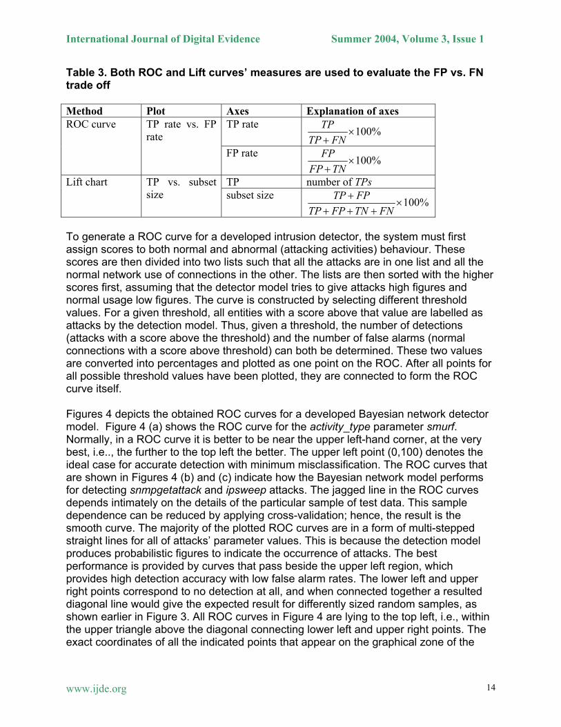
Table 3. Both ROC and Lift curves’ measures are used to evaluate the FP vs. FN trade off Method Plot Axes Explanation of axes

TP rate 100%TP

TP FN×

+

ROC curve TP rate vs. FP rate

FP rate 100%FP

FP TN×

+

TP number of TPs Lift chart TP vs. subset size subset size

100%TP FPTP FP TN FN

+×

+ + +

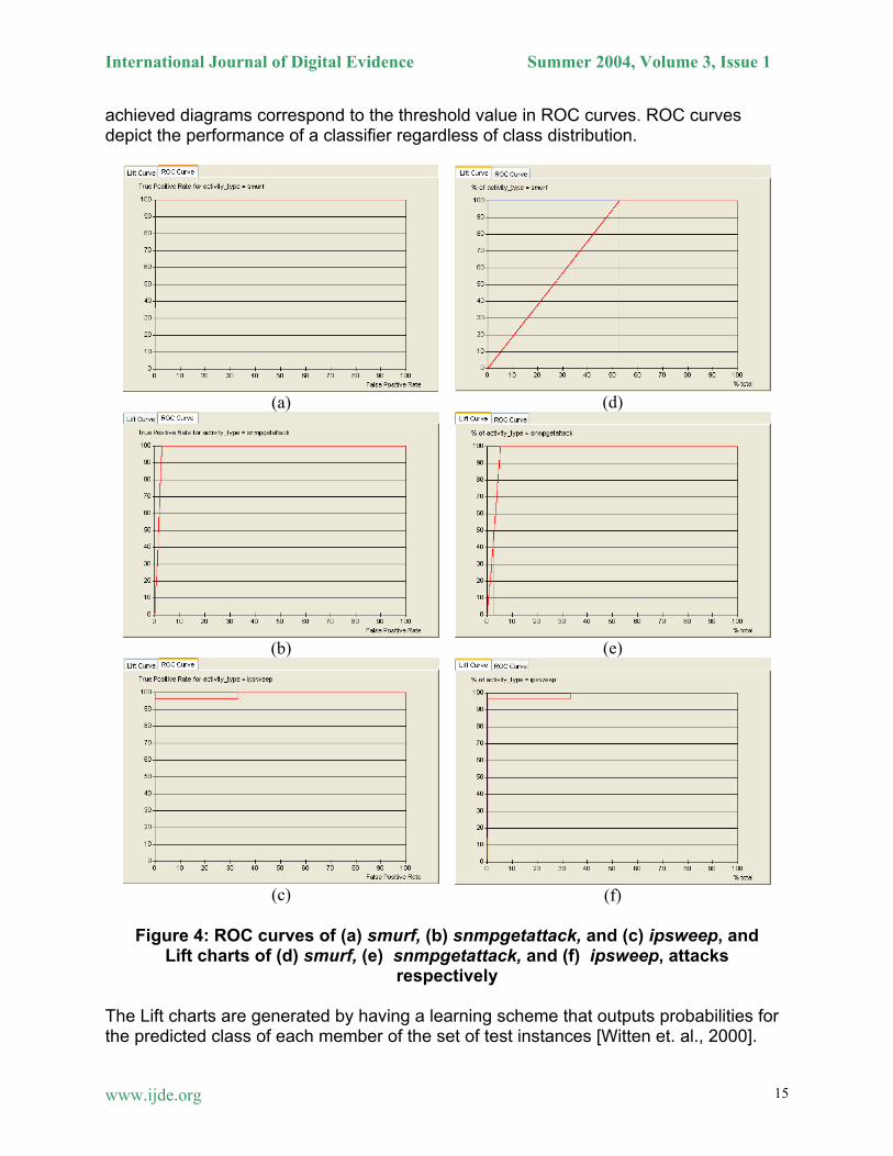
To generate a ROC curve for a developed intrusion detector, the system must first assign scores to both normal and abnormal (attacking activities) behaviour. These scores are then divided into two lists such that all the attacks are in one list and all the normal network use of connections in the other. The lists are then sorted with the higher scores first, assuming that the detector model tries to give attacks high figures and normal usage low figures. The curve is constructed by selecting different threshold values. For a given threshold, all entities with a score above that value are labelled as attacks by the detection model. Thus, given a threshold, the number of detections (attacks with a score above the threshold) and the number of false alarms (normal connections with a score above threshold) can both be determined. These two values are converted into percentages and plotted as one point on the ROC. After all points for all possible threshold values have been plotted, they are connected to form the ROC curve itself. Figures 4 depicts the obtained ROC curves for a developed Bayesian network detector model. Figure 4 (a) shows the ROC curve for the activity_type parameter smurf. Normally, in a ROC curve it is better to be near the upper left-hand corner, at the very best, i.e.., the further to the top left the better. The upper left point (0,100) denotes the ideal case for accurate detection with minimum misclassification. The ROC curves that are shown in Figures 4 (b) and (c) indicate how the Bayesian network model performs for detecting snmpgetattack and ipsweep attacks. The jagged line in the ROC curves depends intimately on the details of the particular sample of test data. This sample dependence can be reduced by applying cross-validation; hence, the result is the smooth curve. The majority of the plotted ROC curves are in a form of multi-stepped straight lines for all of attacks’ parameter values. This is because the detection model produces probabilistic figures to indicate the occurrence of attacks. The best performance is provided by curves that pass beside the upper left region, which provides high detection accuracy with low false alarm rates. The lower left and upper right points correspond to no detection at all, and when connected together a resulted diagonal line would give the expected result for differently sized random samples, as shown earlier in Figure 3. All ROC curves in Figure 4 are lying to the top left, i.e., within the upper triangle above the diagonal connecting lower left and upper right points. The exact coordinates of all the indicated points that appear on the graphical zone of the

www.ijde.org 14


achieved diagrams correspond to the threshold value in ROC curves. ROC curves depict the performance of a classifier regardless of class distribution.

(a) (d)

(b)

(e)

(c) (f)

Figure 4: ROC curves of (a) smurf, (b) snmpgetattack, and (c) ipsweep, and

Lift charts of (d) smurf, (e) snmpgetattack, and (f) ipsweep, attacks respectively

The Lift charts are generated by having a learning scheme that outputs probabilities for the predicted class of each member of the set of test instances [Witten et. al., 2000].

www.ijde.org 15


The next step is to find subsets of test instances that have a high proportion of positive instances, higher than in the test set as a whole. The instances are stored in descending order of predicted probability of yes. Then, to find a sample of a given size with the greatest possible proportion of positive instances, just read the requisite number of instances off the list, starting from the top. If each test instance’s class is known, it is possible to calculate the lift factor by simply counting the number of positive instances that the sample includes, dividing by the sample size to get a success proportion, and dividing by the success proportion for the complete test set to get a lift factor. All these steps were created to generate the Lift charts for each attack category, as shown in the Figures 4 (d), (e) and (f). Figure 4 depicts the obtained Lift charts for the developed Bayesian network detector model. Figure 4 (d) shows the Lift chart for the activity_type parameter smurf. Normally, in a lift chart near the upper left-hand corner is a good place to be, the further to the top left the better. The upper left point (0,100) denotes the ideal case for accurate detection with minimum cost. The Lift charts that are shown in figures 4 (e) and (f) indicate how the Bayesian network model performs for detecting snmpgetattack, and ipsweep attacks. Evaluation Remarks:

• The ROC curves were generated for all the parameter values of targeted variable node activity_type. This node is part of a developed Bayesian detector model and includes different network attack types. All entries in each returned test list file were sorted by attack score, with the highest scores at the top of the list. Scoring was slightly different for the different categories of attacks because DoS and probe attacks sometimes use thousands of network ICMP and UDP packets while others such as U2R and R2L attacks typically only use one or a few TCP protocol connections. This scoring was a fraction of packets associated to each particular attack that occur in the sorted list file above the ROC threshold setting. A threshold was then set to be above the highest score on the list, and then lowered progressively through all entries on the list. At each threshold value, a point on the ROC curve was plotted. This produced the developed detection model that is capable of finding the majority of packets associated with each high traffic probe or DoS attack. The ROC curves’ overall results across all network attacks feature the characteristics of the capability of a developed Bayesian network detector model to identify network anomalies found in the training data, as well as unseen test data.

• Both the generated ROC curves and lift charts of figure 4, represent an effective

measure for the validation of a detection process and whether a given attack classification is valid or not. They also indicate how effective a developed detector model is from the point of view of reducing false alarms. Figure 4 indicates that a developed model led to a substantial reduction of false alarms, with significant increase in detection rates. This verifies that a developed detection technique actually extracted the right anomaly events for enabling

www.ijde.org 16


learning detection. The significance levels on the generated ROC curves and Lift charts can be used as tuning parameters for affecting a trade-off between detection rates (i.e., TPs) and false alarms (i.e., FPs). Larger significance levels lead to higher thresholds, and vice versa, as mentioned earlier.

• The generated ROC curves and Lift charts indicate that each point on every

curve corresponds to drawing a line at a certain position on a developed ranked list and counting the yeses and no’s above it, plotting them vertically and horizontally respectively. A good detection model would give most attacks a high score and most normal connections a low score. Consequently a curve which climbs very sharply to a point with a high detection rate and a low false alarm rate, and then levels out, is a good case. One metric derived from both ROC and Lift chart plots is the area under the curve, where 100% area is a perfect model and 50% is equivalent to random guessing.

When one is faced with the problem of predicting a value of a particular variable (the value of target node), the evaluation of the Bayesian network detection model can be learned from the dataset by using both the number of the processed cases and the number of correct predictions [BayesiaLab, 2003]. For all the cases of the dataset, the probability of the target value is inferred and the cases are stored according to their probability in such a way that the most probable cases are placed at the beginning of the list. With a perfect detection model, the cases with the target value (p % of the population) are then placed in the first p % cases. With a random choice of the cases, the expected detection rate is directly given by the selection rate. If someone randomly selects x% of the cases, the expected detection rate of the cases with the target value is x%. Compare one network intrusion detection system that receives an average of 10,000 packets a minute and is able to detect 10% (1000 packets) as unauthorised traffic, with another that receives an average of 15,000 packets a minute and is able to detect 8% (1200 packets) of unauthorised traffic. Which is better? It always depends on the relative cost of false positives, i.e. packets that are identified as unauthorised that are actually authorised, and false negatives, packets that are identified as authorised that are actually unauthorised. Therefore, ROC curves and Lift charts can be used to compare various intrusion detection models and provide a common approach for future intelligent detectors’ evaluations. However, different intelligent network intrusion detection models are based or trained on different datasets, so it is quite difficult to ensure effective comparison methods unless a common dataset is used for that purpose. Validation Remarks:

• By using the ROC curves and Lift charts to measure the developed detection model performance, the model’s dynamic behaviour of the detection rate has been indicated with respect to the false positives and the sample data accumulated during the simulation time of the complete dataset, taking into

www.ijde.org 17


consideration that only part of the dataset is used for testing purposes. This confirms both of the validation techniques, the operational graphics and historical data validation.

• Using a number of different techniques to measure the performance of the

developed model such as the confusion matrix, ROC curves, and Lift charts, the accuracy of the achieved model’s detection performance is quite promising and encouraging. The achieved high levels of reliability and precision of the developed model’s prediction confirm the Traces and Turing tests’ validation techniques.

The evaluation and validation of any developed detection model has to be done in the presence of both normal and anomaly network traffic. This is to establish the performance of a developed detection model. Without normal traffic the total number of false alarms generated by the model for each attack cannot be identified. Hence, the cost of maintaining the implemented system cannot be identified as well. The generated large corpus of normal, as well as anomaly network traffic, and the developed learning detector model made it possible to do the evaluation and performance measurement. The training data included a few months of background traffic with about 40 different types of automated attacks that were launched against particular victim machines. The training data was labelled indicating attacks, and unlabeled test data was used for a blind evaluation. The ROC curves and Lift charts were able to determine the attack detection rate as a function of the false alarm rate for the previously unseen test data. Results were analysed separately for each individual network attack using confusion matrix, ROC curves and Lift charts. Good use of training data has been made to develop an intelligent networked type detector based on Bayesian learning as a probabilistic approach. Conclusion In this paper, the evaluation methodology used to measure the performance of intelligent intrusion detection models has been discussed. A developed model has been trained to detect, as well as predict, unauthorised activities in networks using Bayesian techniques. The evaluation and validation criteria, as well as the learning prediction performance for this task, have been discussed. The evaluation methodology applied standard criteria to evaluate the performance of a developed Bayesian learning-based anomaly detection model. In conjunction with the achieved statistical measurements, the performance of probabilistic predictions was measured. The evaluation approach covered the measurement of the prediction performance for a developed detector model by, applying the informational loss function, evaluating the precision parameter using the confusion matrix, and measuring the performances of the models and their cost of misclassification using Lift charts and ROC curves which support 10-fold stratified cross-validation. The validation of a developed model is based on various combined techniques acceptable by the Verification and Validation (V&V) community, such as parameter variability-sensitivity analysis, predictive validation, operational graphics, historical data validation, historical methods, multistage validation, traces and Turing

www.ijde.org 18


tests. In order to achieve a significant level of confidence, a careful examination the dataset and related experiments has been carried out. The evaluation and validation of a developed detection model have been conducted to establish and measure the performance of an intelligent detection model. A similar relationship of a developed model change appears in a real EMERALD intrusion detection system as a result of internal parameters changes. However, the Bayesian developed model’s output provides a probabilistic figure to indicate its confirmed prediction. Having a probabilistic figure to indicate for a particular attack occurrence other than a black or white output will help in predicting future similar unauthorised anomalies. Both generated ROC curves and lift charts of figures 4 (a), (b), (c), (d), (e) and (f) respectively, represent an effective measure for the evaluation of the detection process and whether a given attack classification is valid or not. They also indicate how far a developed detector model is effective from the point of view of reducing the false alarms. The achieved results indicate that the developed model led to a substantial reduction of the false alarms, with significant increase in the detection rates. In general, the developed detector model can reliably detect many existing network attacks with low false alarm rates as long as examples of these anomalies are available for training. Also, as a probabilistic based detector, it is able to generalise to new attacks, and therefore, could minimise the false rate for unknown future anomalies. © 2004 International Journal of Digital Evidence About the Authors Nasser S. Abouzakhar is pursuing his PhD research with the Centre for Mobile Communications Research (C4MCR), University of Sheffield, UK. Currently, his research area is mainly focused on applying intelligent and learning Agents solutions to secure telecommunication networks. He received a MSc (Eng) in Data Communications from the University of Sheffield in 2000. He can be contacted at [email protected]. Gordon A. Manson received his B.Sc. degree in 1971 and his PhD in 1977 from Strathclyde University and a M.Sc. in 1983 from the University of Manchester. He is currently a Senior Lecturer in the Department of Computer Science at the University of Sheffield. He was the assistant director of the National Transputer Support Centre 1987-96. For the last 13 years he has worked with Universities and colleges in Malaysia. His current research interests are in Mobile Agents, Dynamic Services and the use of Java technology in wireless and wired networks. He can be reached at [email protected].

www.ijde.org 19

mailto:[email protected]

mailto:[email protected]


www.ijde.org 20

References Amoroso, E. (1999). “Intrusion detection: An Introduction to Internet Surveillance,

Correlation, Trace Back, Traps, and Response.” Intrusion.net. Bace, R. (2000). Intrusion Detection. Macmillan Technical Publishing, USA. BayesiaLab Tutorial (2003). Retrieved June 1, 3004 from http://www.BayesiaLab.com. Kleijnen, J. P. C. (1999). “Validation of Models: Statistical Techniques and Data

Availability,” Proceedings of the Winter Simulation Conference, pp. 647-654. Marchette, D. J. (2001). Computer Intrusion Detection and Network Monitoring: A

Statistical Viewpoint. Springer-Verlag ., New York , USA. MIT Lincoln Lab, retrieved June 5, 2001 from http://www.ll.mit.edu/IST/ideval/index.html.

Naylor, T. H. and Finger, J. M. (1967). “Verification of Computer Simulation Models,”

Management Science, 14:2, B92-B101. O’Connell, B. and Myers, H. (2002). “Information Point: Receiver Operating

Characteristics (ROC) Curves,” Journal of Clinical Nursing, Blackwell Science Ltd., 11, pp.134-136.

Sargent, R. G. (1999). “Validation and Verification of Simulation Models,” Proceedings

of the Winter Simulation Conference, pp. 39-48. Valdes, A. and Skinner, K. (2001). “Probabilistic Alert Correlation,” Lecture Notes in

Computer Science, No. 2212, “Recent Advances in Intrusion Detection” (RAID 2001), Springer-Verlag.

Witten, I. H. and Frank, E. (2000). Data Mining, Practical Machine Learning Tools and

Techniques with Java implementations. Morgan Kaufmann, USA.

http://www.bayesialab.com/

http://www.ll.mit.edu/IST/ideval/index.html

evaluation of intelligent intrusion detection models · evaluation of intelligent intrusion...

Documents