european spatial data research · change detection in high- ... multisource attribute extraction...

Offi cial Publication No 64

European Spatial Data Research

April 2014

Change Detection in High-Resolution Land Use/Land Cover

Geodatabases (at Object Level)Emilio Domenech, Clément Mallet

A survey on state of the art of3D Geographical Information Systems

Volker Walter

Dense Image Matching Final ReportNorbert Haala

Crowdsourcing in National MappingPeter Mooney, Jeremy Morley

The present publication is the exclusive property of European Spatial Data Research

All rights of translation and reproduction are reserved on behalf of EuroSDR. Published by EuroSDR printed by Buchdruckerei Ernst Becvar, Vienna, Austria

EUROPEAN SPATIAL DATA RESEARCH PRESIDENT 2012 – 2014:

Thorben Brigsted Hansen, Denmark VICE-PRESIDENT 2013 – 2017:

André Streilein-Hurni, Switzerland SECRETARY-GENERAL:

Joep Crompvoets, Belgium DELEGATES BY MEMBER COUNTRY:

Austria: Michael Franzen Belgium: Ingrid Vanden Berghe; Jo Vanvalckenborgh Croatia: Željko Hećimović; Ivan Landek Cyprus: Andreas Sokratous, Georgia Papathoma Denmark: Thorben Brigsted Hansen; Lars Bodum Finland: Juha Hyyppä, Jurkka Tuokko France: Benedicte Bucher, Yannick Boucher Germany: Hansjörg Kutterer; Klement Aringer; Lars Bernard Ireland: Andy McGill, Kevin Mooney Italy: Fabio Crosilla, Alesandro Capra Netherlands: Jantien Stoter; Martijn Rijsdijk Norway: Jon Arne Trollvik; Ivar Maalen-Johansen Spain: Antonio Arozarena, Emilio Domenech Sweden: Mikael Lilje Switzerland: Francois Golay; André Streilein-Hurni United Kingdom: Malcolm Havercroft; Jeremy Morley

COMMISSION CHAIRPERSONS:

Sensors, Primary Data Acquisition and Georeferencing: Fabio Remondino, Italy Image Analysis and Information Extraction: Norbert Pfeifer, Austria Production Systems and Processes: Jon Arne Trollvik, Norway Data Specifications: Jantien Stoter, The Netherlands Network Services: Jeremy Morley, United Kingdom

OFFICE OF PUBLICATIONS:

Bundesamt für Eich- und Vermessungswesen Publications Officer: Michael Franzen Schiffamtsgasse 1-3 1020 Wien Austria Tel.: + 43 1 21110 5200 Fax: + 43 1 21110 5202

CONTACT DETAILS:

Web: www.eurosdr.net President: [email protected] Secretary-General: [email protected] Secretariat: [email protected] EuroSDR Secretariat Public Management Institute K.U. Leuven Faculty of Social Sciences Parkstraat 45 Bus 3609 3000 Leuven Belgium Tel.: +32 16 323180

The official publications of EuroSDR are peer-reviewed.

(a) Emilio Domenech, Clément Mallet:„Change Detection in High-Resolution Land Use/Land Cover Geodatabases (at Object Level)“ ................................................................................................... 9

1. Introduction ..................................................................................................................... 11

2. Objectives ........................................................................................................................ 12

3. Study areas and data pre-processing ............................................................................... 12

3.1. Alcalá de Henares data ....................................................................................... 143.2. Valencia data ...................................................................................................... 143.3. Murcia data ......................................................................................................... 16

4. Methodology ................................................................................................................... 16

4.1. Classificationinbasiclandcover ....................................................................... 174.1.1. Image segmentation ............................................................................... 184.1.2. Region adjacency graph ........................................................................ 204.1.3. ImageclassificationimprovementusingDempster-Shafertheory ........ 214.1.4. Shadow removal .................................................................................... 24

4.1.4.1. Computing the shadow layer .................................................... 244.1.4.2. Assigning classes to shadow regions ........................................ 25

4.2. Multi-sourceattributeextractionandlanduseclassification ............................. 274.2.1. Feature extraction .................................................................................. 28

4.2.1.1.LiDAR-basedfeatures .............................................................. 304.2.1.2.Spatialcontextfeatures ............................................................ 31

4.2.2. Objectclassification .............................................................................. 314.2.2.1.Objectandclassdefinition ....................................................... 314.2.2.2.Selectionofdescriptivefeatures ............................................... 334.2.2.3.Classificationprocedure ........................................................... 35

4.3. Change detection ................................................................................................ 364.3.1. Change detection evaluation ................................................................. 36

5. Results ............................................................................................................................. 38

5.1. PhaseIresults:generationofbasiclandcoverclasses ...................................... 385.2. PhaseIIresults:multisourceattributeextractionandlanduseclassification .... 415.3. Change detection results .................................................................................... 45

5.3.1. Change detection in periurban areas ..................................................... 455.3.2. Change detection in rural areas ............................................................. 46

5.4. ApplicationtoquantifypolygonattributesinSIOSEdatabase ......................... 48

6. Conclusions ..................................................................................................................... 54

7. Future Studies ................................................................................................................. 54

8. References ....................................................................................................................... 57

(b) Volker Walter:„Asurveyonstateoftheartof3DGeographicalInformationSystems“ .................................... 65

1 Introduction ..................................................................................................................... 66

2 Participants ...................................................................................................................... 66

3 EvaluationofQuestionnairePartA ................................................................................. 68

4 QuestionnairePartB ....................................................................................................... 82

5 Summary ......................................................................................................................... 86

6 Conclusions and Outlook ................................................................................................ 86

Annex A: Participating Institutions ................................................................................. 88

(c) Norbert Haala:„Dense Image Matching Final Report“ ...................................................................................... 115

1 Introduction ................................................................................................................... 116

2 TheEuroSDRProjectonDenseImageMatching–Datasetsanddeliverables ........... 117

3 Testparticipants,investigatedsoftwaresystemsandusedhardwareenvironment ...... 120

4 EvaluationofDSMQuality .......................................................................................... 122

4.1. TestareaVaihingen/Enz ................................................................................... 1234.2. Test area München ........................................................................................... 133

5 Conclusions ................................................................................................................... 142

6 References ..................................................................................................................... 143

(d) Peter Mooney, Jeremy Morley:„Crowdsourcing in National Mapping“ ..................................................................................... 147

Abstract ...................................................................................................................................... 148

Acknowledgement ..................................................................................................................... 149

Preface148

1 Introduction and Motivation ......................................................................................... 150

2 Project Development Timeline ...................................................................................... 151

3 Projectsselectedforfunding ......................................................................................... 153

4 DetailsofIndividualProjectReports ............................................................................ 154

4a: Project1:Collectionandvisualizationofalternativetourismsites and objects in Lithuania ................................................................................... 155

4.b Project 2: Incidental Crowdsourcing ................................................................ 1574.3: Project 3: Ontology based Authoritative and Volunteered Geographic

Information(VGI)integration .......................................................................... 1584.4 Project4:ConflationofCrowdsourcedData ................................................... 1604.5 Project5:Characterisingtheuseofvernacularplacenamesfromcrowd

sourced data and a comparison with NMA Data .............................................. 162

5 Conclusions and Recommendations. ............................................................................ 164

References .................................................................................................................................. 166

115

EuroSDR-Project Commission 2

“Benchmark on Image Matching” Final Report

Report by Norbert Haala Institute for Photogrammetry, University of Stuttgart

116

Abstract Both improvements in camera technology and the rise of new matching approaches triggered the development and upgrade of suitable tools for image based 3D reconstruction by research groups and vendors of photogrammetric software. Meanwhile, dense pixel-wise matching enables the photogrammetric generation of dense 3D point clouds and Digital Surface Models from highly overlapping aerial images. In order to evaluate the quality of these matching algorithms in terms of accuracy and reliability, the European Spatial Data Research Organisation (EuroSDR) initiated a benchmark on image based DSM generation in February 2013. The test is based on two representative image blocks to be processed by different groups with their respective software systems. By compiling these results, this report aims to provide a profound insight to the landscape of dense matching algorithms while evaluating the current potential of image based photogrammetric data collection.

Preface

A first EuroSDR project on Benchmarking of Image Matching Approaches for DSM Computation was already launched in 2010 by Marc Pierrot Deseilligny and Grégoire Maillet (IGN). This project ended after the EuroSDR Commission II workshop on High Density Image Matching for DSM Computation, in February 2012 (EuroSDR 2012). Also motivated by the success of this workshop, EuroSDR started the follow up project Benchmark on Image Matching in October 2012. This project was led by the principals Prof. Dr. Norbert Haala, Institute for Photogrammetry, Stuttgart University, Wolfgang Stoessel, Landesamt für Vermessung und Geoinformation Bayern (LVG) and Dr. Michael Gruber, Microsoft Photogrammetry. This one year project phase is now concluded by the submission of this final report.

1 Introduction

Recent innovations in matching algorithms considerably improved the quality of elevation data derived from aerial images. Traditional stereo-matching, originally introduced more than two decades ago, typically applies feature based algorithms. These algorithms first extract feature points and then search the corresponding features in the overlapping images (Heipke 1993). The restriction to matches of selected points helps to provide correspondences at high certainty. Additionally, it avoids problems due to limited computational resources, which originally was another motivation to use such feature based matching approaches. In contrast, recent stereo algorithms aim on dense, pixel-wise matches. By these means 3D point clouds and Digital Surface Models (DSM) are generated at a resolution, which corresponds to the ground sampling distance GSD of the original images. To enable pixel matches even for regions with very limited texture, additional constraints are required. Local or window based algorithms like correlation use an implicit assumption of surface smoothness since they compute a constant parallax for a window with a certain number of pixels. In contrast, so-called global algorithms use an explicit formulation of this smoothness assumption, (Szeliski, 2010). The resulting global optimization problem can for example be solved very efficiently by recursive algorithms like scanline optimization. A very popular and well performing approach in this context is semi-global matching (Hirschmüller, 2008). It evaluates a cumulative cost function from multiple scanline directions. The approach produces accurate results very efficiently, especially when combined with sophisticated aggregation strategies (Szeliski, 2010). Thus, this technique is currently

117

implemented by a number of research institutes and photogrammetric software vendors within their software tools for image based 3D point cloud generation. These developments are considerably changing the landscape of photogrammetric data processing. Especially during such stages of rapid progress, benchmarks which measure the performance of state-of-the-art algorithms have proven to be extremely useful for supporting the further development. Well known examples in the context of matching algorithms are the Middlebury Stereo Vision Page (Scharstein, & Szeliski 2002) or the benchmark on multi-view stereo reconstruction (Seitz et.al. 2006). These benchmarks provide general purpose datasets through a platform, which additionally allows for an upload of the results by the respective participant. These are then compared to available reference data to compute suitable quality metrics. While these projects emerged from the Computer Vision community, a test on the performance of photogrammetric digital airborne camera systems was organized under the umbrella of the German society of Photogrammetry, Remote Sensing and Geoinformation (DGPF) by Cramer (2010). There the potential of photogrammetric 3D data capture from automatic image matching was already demonstrated by Haala et.al. (2010). Also in view of the rapid progress in software technology, EuroSDR started another initiative to evaluate the ongoing developments in image based DSM generation in October 2012. The benchmark was announced via the EuroSDR web-page (EuroSDR, 2013a), which was also used to disseminate the test data sets to potential participants. Based on the given images and camera parameters, test participants then had the opportunity to produce Digital Surface Models with their software system. After the results were sent back, the project team started further evaluation. These results were presented and discussed during the 2nd EuroSDR workshop on High Density Image Matching for DSM Computation held from 13th to 14th June 2013 at the Federal Office for Metrology and Surveying in Vienna (EuroSDR 2013b). There the respective groups could demonstrate their state-of-the-art in high quality image based DSM generation and discuss future applications and additional needs together with potential users. Since the workshop brought together software developers, distributors and users of dense matching software it was a very suitable platform for a first review on the outcomes of the benchmark. The following section of this report first presents the test data sets, which consists of image blocks for two representative areas. Section 3 then introduces the different software systems used during the test while section 4 compares, evaluates and discusses the respective results from these software systems as generated by the test participants.

2 The EuroSDR Project on Dense Image Matching – Data sets and deliverables In order to limit the effort required for data processing by potential benchmark participants, the test was restricted to two subsets of aerial image flights. To achieve representative data sets, two aerial image sub-blocks of different landuse and block geometry were selected. The first data set, Vaihingen/Enz is an example for data typically collected during state-wide DSM generation at areas with varying landuse. As it is visible from the ortho image and the DSM of the test area in Figure 1 it covers a semi-rural area at undulating terrain. Elevation differences of 200m occur between the river valley and the upper area. The data are a subset from a flight collected during the project on Digital Airborne Camera Evaluation of the German Society of Photogrammetry, Remote Sensing and Geoinformation (DGPF) (Cramer, 2010).

118

Figure 1: Vaihingen/Enz test area with ortho image and DSM. Both ground sampling distance (GSD)and overlap of the image block are rather moderate. This situation is typical for most flights captured for national mapping agencies. The aerial images were captured by an UltraCam-X at height above ground of 2900m and a GSD of 20cm. For image matching the PAN images had to be used, which were made available as Tiled Tiff uncompressed 8 bit/pix with 9420x14430pix at 136Mpix/image.

Figure 2: Vaihingen/Enz: Image overlap (maximum nine-folded) with image footprints and camera stations. The area to be processed is depicted as light blue rectangle

119

The sub-block selected for the benchmark is depicted in Figure 2. It consists of 3 strips with 10 images each. Figure 2 additionally visualizes the corresponding 30 camera stations, which are represented by the blue points. The respective image footprints are depicted by rectangles in the same color. One of the main factors which influence the quality of image based surface reconstruction is the amount of image overlap. In Figure 2 the number of images available for each terrain point is represented by the color coded map. For the Vaihingen/Enz sub-block, the available overlap of 63% in flight and 62% cross flight results in variations from one-folded areas (red) to nine-folded overlap (green). In Figure 2 these areas are represented in red and dark green, respectively. As it is also visible, usually four to nine images were available for the central part of the block, where the DSM had to be generated. During the test a DSM had to be generated for the central part of the block at a size of 7.5kmx3.0km. This part is highlighted by the rectangle with light blue outlines and corresponds to the ortho image and DSM already shown in Figure 1. Participants of the benchmark were asked to generate a DSM raster at a grid with of 0.2m, which resulted in a DSM raster of 37500x15000 pixels.

Figure 3: München test area with DSM (left) and color-coded image overlap (maximum 15 folded) with image footprints, camera stations and area to be processed (right).

The second test area München is representative data collection in densely built-up urban areas. For such applications, images are usually captured at a higher overlap and resolution. As it is visible from the grey coded DSM representation in Figure 3 (left), this urban data set covers the central part of the city at a size of 1.5kmx1.7km. The imagery was captured by a DMC II 230 camera at a GSD of 10cm. Each image has a size of 220 Mpixel/image (15552x14144 pix) at 16 bit/pix. The image sub-block to be processed consists of 3 image strips with 5 images each. In the right part of Figure 3, the camera stations are represented by dark blue triangles with the corresponding image footprints depicted as rectangles in the same color. The area to be processed is highlighted by the light blue rectangle. The image block was captured with 80% in flight and 80% cross flight overlap, which results in up to fifteen-folded object points in the central part of the test area. In Figure 3 (right) this maximum overlap is depicted in dark green. This large overlap provides a considerable redundancy during DSM generation. However, it reduces to five images per object pixel at the border of the area to be processed.

120

Figure 4: Visualisation of test area München A textured DSM visualization for a part of the test area München is given in Figure 4. As it is visible, the area is rather flat but densely covered by buildings with heights of up to 50m. Thus, surface parts close to the building facades will frequently be subject to occlusions. This potentially aggravates the matching processes during DSM generation for such regions.

3 Test participants, investigated software systems and used hardware environment

To address a suitable number of participants, the test procedure for the benchmark was kept relatively simple. Since the main focus is on dense image matching, all participants had to use the orientation parameters made available for the image blocks without modification. Participants had to compute a DSM raster of predefined size and resolution as their final outcome. These results were then sent to the project team for comparison and accuracy analysis. In addition to the required processing time, the participants were asked to provide further information on their available hardware environment and their processing strategy. These informations were retrieved by a questionnaire and also presented by the participants during the 2nd EuroSDR workshop on High Density Image Matching for DSM Computation. The following list briefly summarizes this information for each software system.

• SocetSet 5.6 (NGATE) from BAE Systems was presented by C. Ginzler from Swiss Federal Institute for Forest, Snow and Landscape Research (WSL). He used an Intel Xeon CPU X5570 2.93 GHz and 24 GB memory. The required processing time for Vaihingen/Enz was 36h and 25h for München. • B. Brunner from Forest Mapping and Management (FMM) Salzburg presented results from Microsoft UltraMap V3.1. This software can only be used from imagery captured by the UltraCam product family. Therefore, investigations were restricted to the Vaihingen/Enz data set. Furthermore, processing has to pass through all software modules. Since this includes Automatic Aerial Triangulation and color adjustment, the UltraMap results are based on an individual bundle block adjustment. Furthermore instead of the 8bit images

121

provided to the participants the originally 16bit imagery was used. The IT environment consisted of 32 Xeon E5-2630/i7 cores and 5 GPU`s (1 Tesla K10, 4 Tesla M2090). For the 36 images of the Vaihingen/Enz block this comparable powerful environment resulted in a processing time of about 35min for data ingest and AAT while the DSM was computed in 27min. • Match-T DSM 5.5 from Trimble/inpho was presented by C. Ressl from the Department of Geodesy and Geoinformation (GEO) at TU Wien. He used an Intel Core i7 CPU, 3GHz with 4 cores and 8GB memory. Match-T itself matches only one image pair for each XY-location. To exploit the high image overlap all possible image pairs where matched during his investigations. The resulting DSMs were then fused using the in-house software systems Opals. Processing time for Vaihingen/Enz resuled in 23h for matching with Match-T and 38h for data import, gridding and fusion with Opals. For the München data set the numbers were 19h for matching with Match-T and 37h for processing with Opals. • The ImageStation ISAE-Ext software was demonstrated by R. Schneider from GEOSYSTEMS GmbH, Germany. For the München test area processing was limited to 6 stereo models. The hardware environment of 2 Intel Xeon Quadcore Processors with 16GB RAM a computation time of 40min per stereo model and 4h for the complete block was achieved. For Vaihingen/Enz 33 stereo models were processed at an average computation time per stereo model of 20min. This resulted in 11h for stereo matching in total, followed by 21h for grid interpolation of the 580 million points to the required 20cm raster. • P. Nonin from Astrium GEO-Information Services presented results for the Pixel Factory software. For his investigations a hardware configuration of 2 Xeon E5-2640, 2.5GHz with 2x6 cores was used. Results for the München area are based on the processing of 12 stereo pairs. Due to expected problems from moving shadows no cross-track matching was applied for this scene. Total time for DSM generation was 2h 12min. For Vaihingen/Enz 57 stereo pairs were processed in a total time of 3h 9min. • M. Idrissa from the Royal Military Academy (RMA), Brussels showed results for the RMA DSM Tool. For processing a Linux Cluster with more than 90 Fedora CPUs (Intel – 2.4 GHz) and more than 30 nodes with 272GB RAM (total) and a 1000Mbit/s network was used. Processing times for München was approximately 18min per stereo couple and about 5h for the complete block, for Vaihingen/Enz the numbers were 8min per stereo pair and again 5h in total. • Results of the Remote Sensing software package from Joanneum Research, Graz, were presented by K. Gutjahr. He used a Windows PC Intel Xeon CPU E5-2650, 2.0 GHz with 16 Cores and 32GB RAM for processing. Processing time for Vaihingen/Enz for 57 stereo pairs summed up to 17h 17min for the processing steps preparation, normalization and prediction, matching, forward intersection, DSM generation and DSM finalization. Accordingly the processing time for München with 22 stereo pairs was 21h 39min. • The software system MicMac developed at IGN France was presented by M. Pierrot-Deseilligny. Within MicMac multi image matching is realized by energy minimization either using graph cut or a modified dynamic programming/SGM approach. Vaihingen/Enz was processed within 6h and München in 12h. • M. Rothermel presented results from the SURE software developed at the Institute for Photogrammetry (IfP), University of Stuttgart. It is based on a SGM variant with integrated coarse-to-fine strategy based on efficient implementation of SGM on dynamic data structures. He used a PC with one i7 CPU quadcore at 3.4GHz and 32GB Ram. For the

122

München data set in total 4h 13min were required. The processing time for Vaihingen/Enz summed up to 4h 37min. For an alternative implementation using an NVIDIA 580 GTX GPU and an i3 CPU, dual-core the Vaihingen/Enz data set was processed in 2h 50min. • H. Hirschmüller, German Aerospace Center (DLR) provided results from a FPGA implementation of his SGM algorithm. Processing was realized on an Intel Xeon E5-1620 quad core PC. However, for processing a Virtex 6 FPGA board with 8GB Ram, connected to the PC via GigE was applied. With this configuration a processing time for the München data set of 5h 51min and 19h 31min for Vaihingen/Enz was recorded. These results were available before the workshop, however, no presentation was given • Results from Leica’s XProSGM, which is included within Intergraph ImageStation’s ISAE-Ext for dense matching was provided after the workshop by Stephan Gehrke. Processing was realized for Munich on a i7-920 CPU quadcore at 2.67GHz, for the Vaihingen/Enz area on a i7-2600 at 3.4GHz. For Munich a total of 42 stereo pairs were processed to generate the DSM in 50.3 hours, for Vaihingen/Enz 87 image pairs were used in a processing time of in 26.8 hours. In this research project commercial photogrammetric software systems were used by customers and vendors. Scientific staff from research institutes tested their self-developed systems. Typically, these software systems were developed for in house production and projects and then made available for the public under different license models. The above compilation also shows that very heterogeneous hardware environments were used during processing. It spread from standard desktop PCs with single to multi core to the use of low-end to multiple high-end graphics cards to the application of computer clusters. Due to the considerable amount of data to be processed, time required for DSM computation is additionally influenced by reading and writing operations. Thus, efficiency of data ingest also depends on the available storage system and network environment. Finally, processing time is influenced by adjusting the respective strategy, which e.g. defines the required amount of stereo-pairs to be processed. As an example, some of the participants have used cross-track matching i.e. images from different strips to form stereo pairs, while others have only used stereo pairs from the same strip for the matching. This is the reason why the reported processing times should not be regarded as a fixed number but as a hint to the capacity of the area covering data collection of the respective software systems. Further information is also available from the presentations in the workshop proceedings (Fritsch et. al., 2013).

4 Evaluation of DSM Quality

In order to assess the quality of DSM data sets, a comparison to a reference surface is most suitable. In principle airborne LiDAR can provide the required independent measurements. However, differences of DSM from image matching to such a reference surface cannot exclusively be put to errors of the matching process. Deviations can for example occur due to a time gap between image and LiDAR data acquisition. For the Vahingen/Enz test area LiDAR and imagery were captured with a lag of 4 weeks. This resulted in considerable elevation differences due to plant growth and harvesting (Haala et.al. 2010). Height variations can additionally result from the different measurement principles. Light pulses from airborne laser scanning partially penetrate a tree canopy, while matching will most probably relate to the visible surface. Finally, pixel-wise matching reconstructs surface representations at a resolution, which is frequently not available from standard LiDAR flights. For Vaihingen/Enz the benchmark aimed at a 20cm grid width of the DSM. This

123

corresponds to 25pts/m2, while LiDAR data was only available with a point density of 6.7 pts/m2. Similarly, the 10cm grid to be generated for München equals to 100pts/m2, while the available LiDAR points have a density of 4 pts/m2. Due to these difficulties in providing suitable ground truth from independent LiDAR measurements, an alternative approach was followed. The reference surface used for our investigations is based on a median DSM, which was computed from the results of all participants. While this median DSM does not provide independent ground truth at a higher order accuracy it still can be used very well to illustrate differences between the respective solutions.

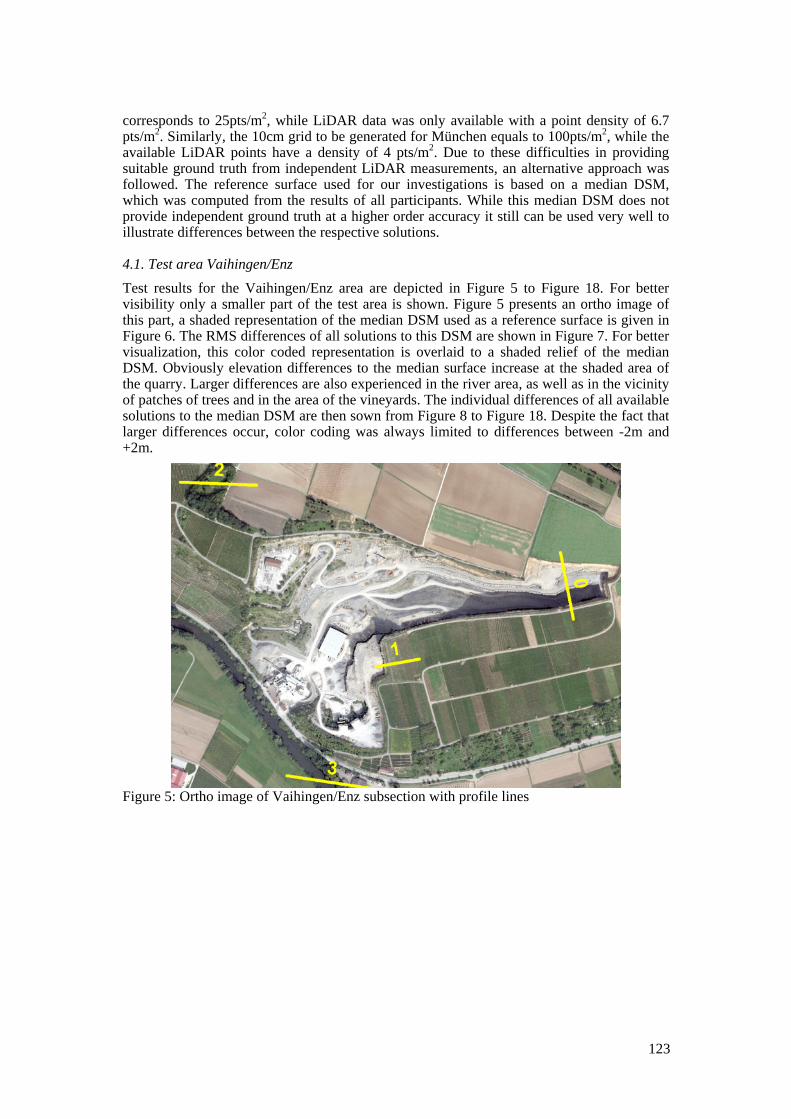
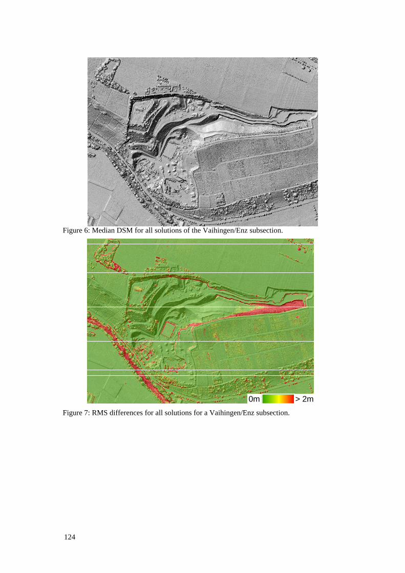
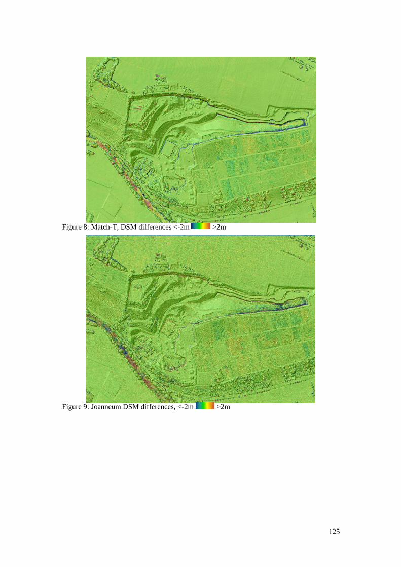
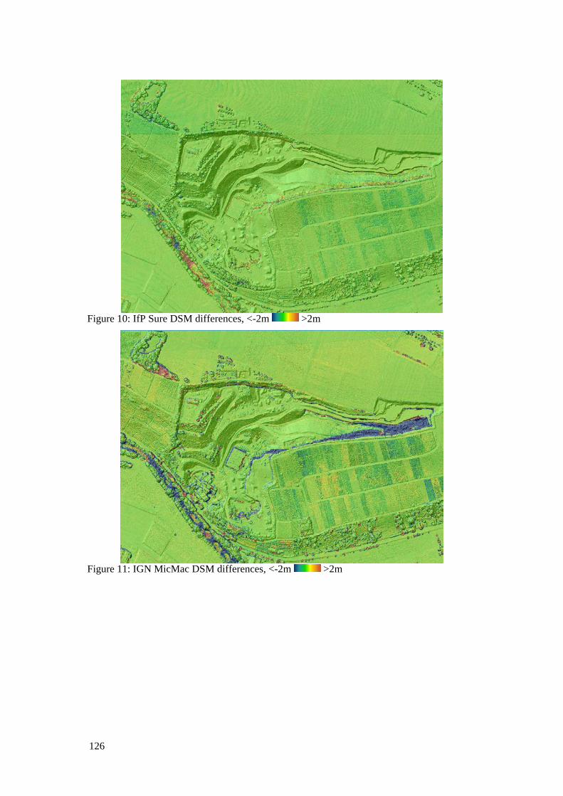
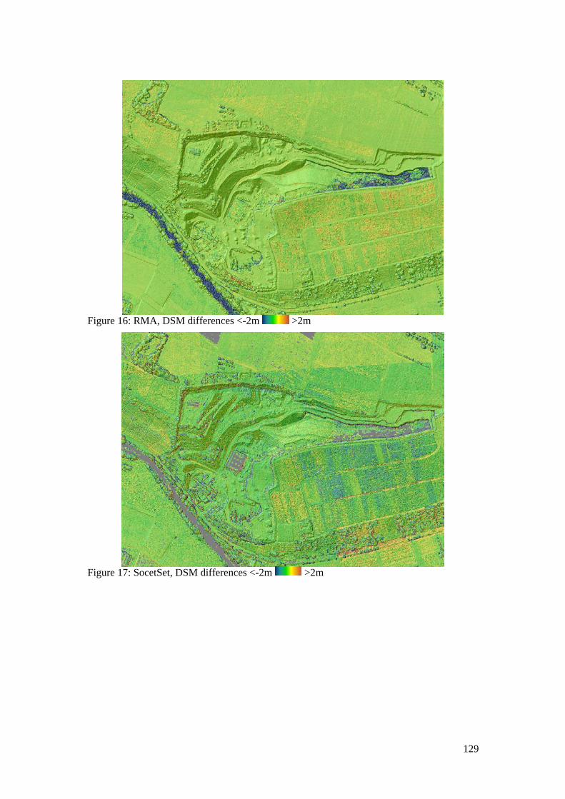
4.1. Test area Vaihingen/Enz Test results for the Vaihingen/Enz area are depicted in Figure 5 to Figure 18. For better visibility only a smaller part of the test area is shown. Figure 5 presents an ortho image of this part, a shaded representation of the median DSM used as a reference surface is given in Figure 6. The RMS differences of all solutions to this DSM are shown in Figure 7. For better visualization, this color coded representation is overlaid to a shaded relief of the median DSM. Obviously elevation differences to the median surface increase at the shaded area of the quarry. Larger differences are also experienced in the river area, as well as in the vicinity of patches of trees and in the area of the vineyards. The individual differences of all available solutions to the median DSM are then sown from Figure 8 to Figure 18. Despite the fact that larger differences occur, color coding was always limited to differences between -2m and +2m.

Figure 5: Ortho image of Vaihingen/Enz subsection with profile lines

124

Figure 6: Median DSM for all solutions of the Vaihingen/Enz subsection.

0m > 2m

Figure 7: RMS differences for all solutions for a Vaihingen/Enz subsection.

125

Figure 8: Match-T, DSM differences <-2m >2m

Figure 9: Joanneum DSM differences, <-2m >2m

126

Figure 10: IfP Sure DSM differences, <-2m >2m

Figure 11: IGN MicMac DSM differences, <-2m >2m

127

Figure 12: GeoSystems DSM differences, <-2m >2m

Figure 13: UltraMap DSM differences, <-2m >2m

128

Figure 14: DLR-SGM DSM differences <-2m >2m

Figure 15: Astrium Pixel-Factory, DSM differences <-2m >2m

129

Figure 16: RMA, DSM differences <-2m >2m

Figure 17: SocetSet, DSM differences <-2m >2m

130

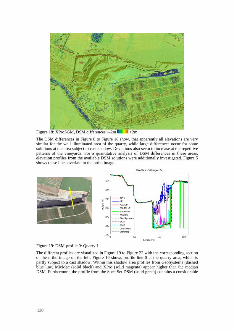
Figure 18: XProSGM, DSM differences <-2m >2m The DSM differences in Figure 8 to Figure 18 show, that apparently all elevations are very similar for the well illuminated area of the quarry, while large differences occur for some solutions at the area subject to cast shadow. Deviations also seem to increase at the repetitive patterns of the vineyards. For a quantitative analysis of DSM differences in these areas, elevation profiles from the available DSM solutions were additionally investigated. Figure 5 shows these lines overlaid to the ortho image.

0 50 100 150250

260

270

280

290

300

310

Lenght [m]

Hei

ght [

m]

Profiles Vaihingen 0

XProIfPAstriumMATCH-TSocetSetMicMacGeoSystemsDLRRMAJoanneumUltraMap

Figure 19: DSM-profile 0: Quarry 1 The different profiles are visualized in Figure 19 to Figure 22 with the corresponding section of the ortho image on the left. Figure 19 shows profile line 0 at the quarry area, which is partly subject to a cast shadow. Within this shadow area profiles from GeoSystems (dashed blue line) MicMac (solid black) and XPro (solid magenta) appear higher than the median DSM. Furthermore, the profile from the SocetSet DSM (solid green) contains a considerable

131

amount of no-data areas. The RMA profile (dashed light blue) is relatively noisy, while for Astrium (solid red) a certain smoothing can be observed.

10 20 30 40 50 60 70 80 90 100

284

286

288

290

292

294

296

298

300

302

304

Lenght [m]

Hei

ght [

m]



30 35 40 45 50 55 60

301

301.5

302

302.5

303

303.5

304

304.5

Lenght [m]

Hei

ght [

m]



Figure 20: DSM-profile 1: Quarry 2 and vineyard Figure 20 shows profile 1, located at another slope of the quarry. In contrast to profile 0 the complete area is well illuminated. Apparently, this is beneficial for the DSM generation. Except for a no-data area from SocetSet, all solutions are relatively consistent. The profiles additionally cover a vineyard. This part is depicted in a more detailed view in the bottom of Figure 20. Apparently this type of landuse increases the differences between the respective solutions. This is possibly due to the fact that the depicted rows of vines have a size close to the 20cm GSD of the available imagery. Still, some solutions like Astrium (solid red), MicMac (solid black), and IfP-SURE (solid blue) at least partially resolve these structures. Furthermore, almost all solutions are able to reconstruct the shape of the small hut in the center of the scene. At such an object surface which is not subject to problems for image matching, differences between almost all solutions are in the pixel level of 20cm.

132

0 20 40 60 80 100 120 140 160

354

356

358

360

362

364

366

368

370

372

Lenght [m]

Hei

ght [

m]



Figure 21: DSM-profile 2: Trees Profile 2 in Figure 21 is situated at an area with patches of trees. Differences between the respective solutions mainly occur at the tree borders, for the bald earth on the right part of the profile results are remarkably consistent. Still, the profile from DLR (dashed red) has a constant offset compared to all other solutions. This is also visible in the difference image of Figure 14. The offset did not occur for a DSM additionally provided by DLR from a CPU based solution. However, the supposed problem in the investigated FPGA solution could not be fixed before finalizing the benchmark.

0 50 100 150 200 250245

250

255

260

265

270

275

Lenght [m]

Hei

ght [

m]



Figure 22: DSM-profile 3: Building and water The final profile investigated for the test area Vaihingen/Enz is shown in Figure 22. The first part covers some buildings on the right and then crosses the river. Since water surfaces are almost impossible to reconstruct from image matching, larger differences of the DSMs occur. However, the solution from UltraMap (dashed black) is remarkably smooth. This is already obvious from the RMS differences of all solutions in Figure 7.

133

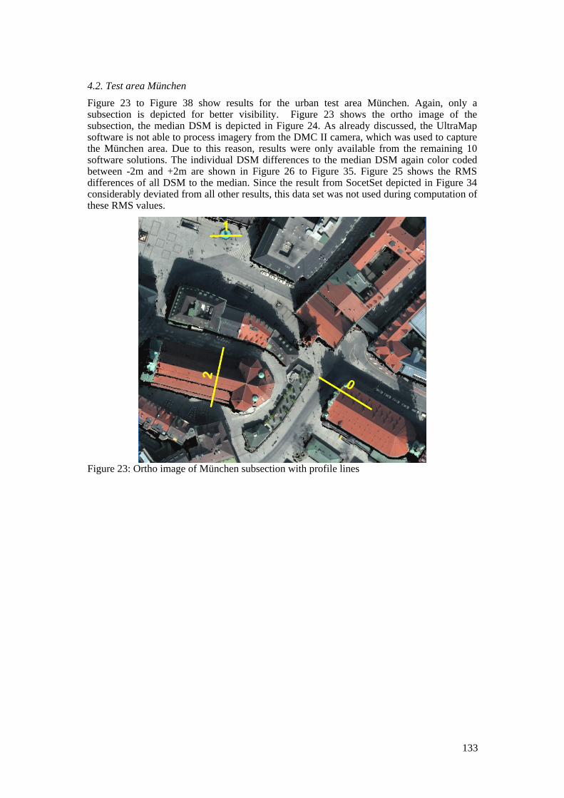
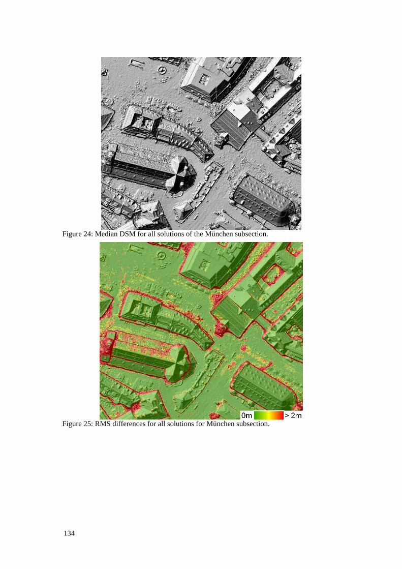
4.2. Test area München Figure 23 to Figure 38 show results for the urban test area München. Again, only a subsection is depicted for better visibility. Figure 23 shows the ortho image of the subsection, the median DSM is depicted in Figure 24. As already discussed, the UltraMap software is not able to process imagery from the DMC II camera, which was used to capture the München area. Due to this reason, results were only available from the remaining 10 software solutions. The individual DSM differences to the median DSM again color coded between -2m and +2m are shown in Figure 26 to Figure 35. Figure 25 shows the RMS differences of all DSM to the median. Since the result from SocetSet depicted in Figure 34 considerably deviated from all other results, this data set was not used during computation of these RMS values.

Figure 23: Ortho image of München subsection with profile lines

134

Figure 24: Median DSM for all solutions of the München subsection.

Figure 25: RMS differences for all solutions for München subsection.

135

Figure 26: Match-T, DSM differences <-2m >2m

Figure 27: Joanneum research DSM differences <-2m >2m

136

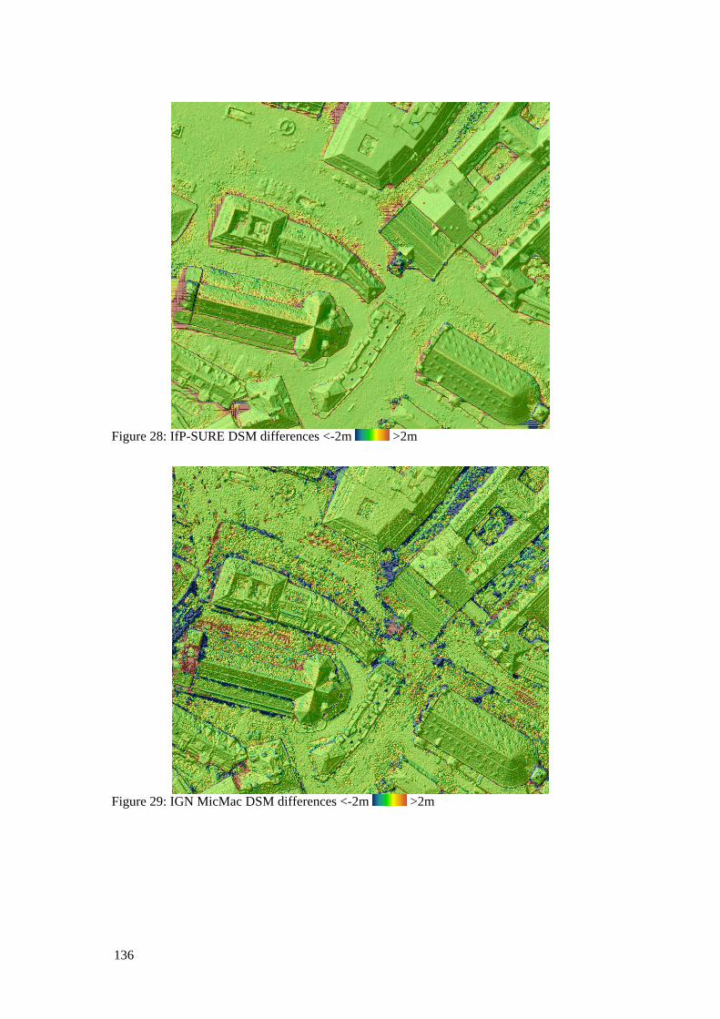
Figure 28: IfP-SURE DSM differences <-2m >2m

Figure 29: IGN MicMac DSM differences <-2m >2m

137

Figure 30: GeoSystems DSM differences <-2m >2m

Figure 31: DLR DSM differences <-2m >2m

138

Figure 32 Astrium Pixel-Factory differences <-2m >2m

Figure 33: RMA differences <-2m >2m

139

Figure 34: SocetSet differences <-2m >2m

Figure 35: XProSGM differences <-2m >2m

140

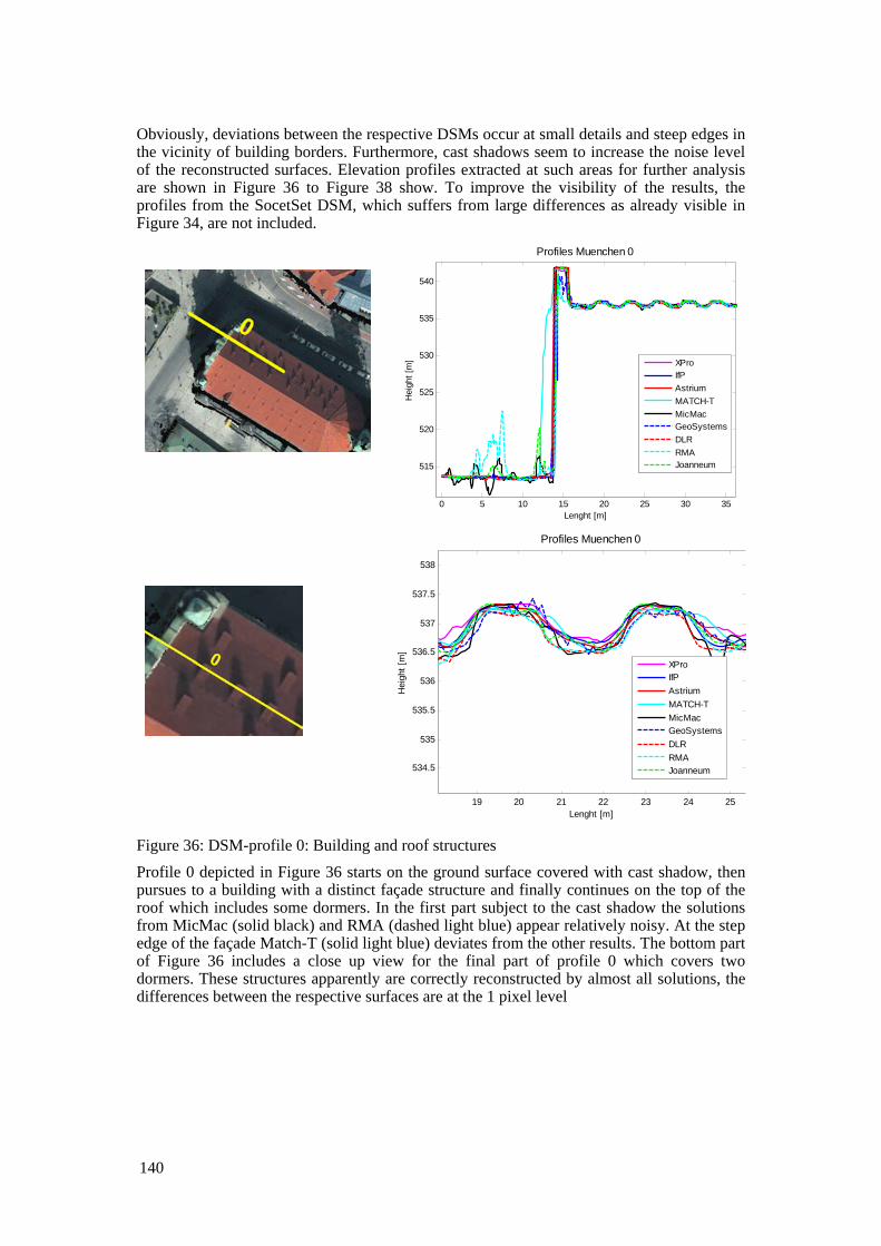
Obviously, deviations between the respective DSMs occur at small details and steep edges in the vicinity of building borders. Furthermore, cast shadows seem to increase the noise level of the reconstructed surfaces. Elevation profiles extracted at such areas for further analysis are shown in Figure 36 to Figure 38 show. To improve the visibility of the results, the profiles from the SocetSet DSM, which suffers from large differences as already visible in Figure 34, are not included.

0 5 10 15 20 25 30 35

515

520

525

530

535

540

Lenght [m]

Hei

ght [

m]

Profiles Muenchen 0

XProIfPAstriumMATCH-TMicMacGeoSystemsDLRRMAJoanneum

19 20 21 22 23 24 25

534.5

535

535.5

536

536.5

537

537.5

538

Lenght [m]

Hei

ght [

m]

Profiles Muenchen 0


Figure 36: DSM-profile 0: Building and roof structures Profile 0 depicted in Figure 36 starts on the ground surface covered with cast shadow, then pursues to a building with a distinct façade structure and finally continues on the top of the roof which includes some dormers. In the first part subject to the cast shadow the solutions from MicMac (solid black) and RMA (dashed light blue) appear relatively noisy. At the step edge of the façade Match-T (solid light blue) deviates from the other results. The bottom part of Figure 36 includes a close up view for the final part of profile 0 which covers two dormers. These structures apparently are correctly reconstructed by almost all solutions, the differences between the respective surfaces are at the 1 pixel level

141

0 2 4 6 8 10 12 14 16 18 20515

515.5

516

516.5

517

517.5

518

518.5

Lenght [m]H

eigh

t [m

]

Profiles Muenchen 1


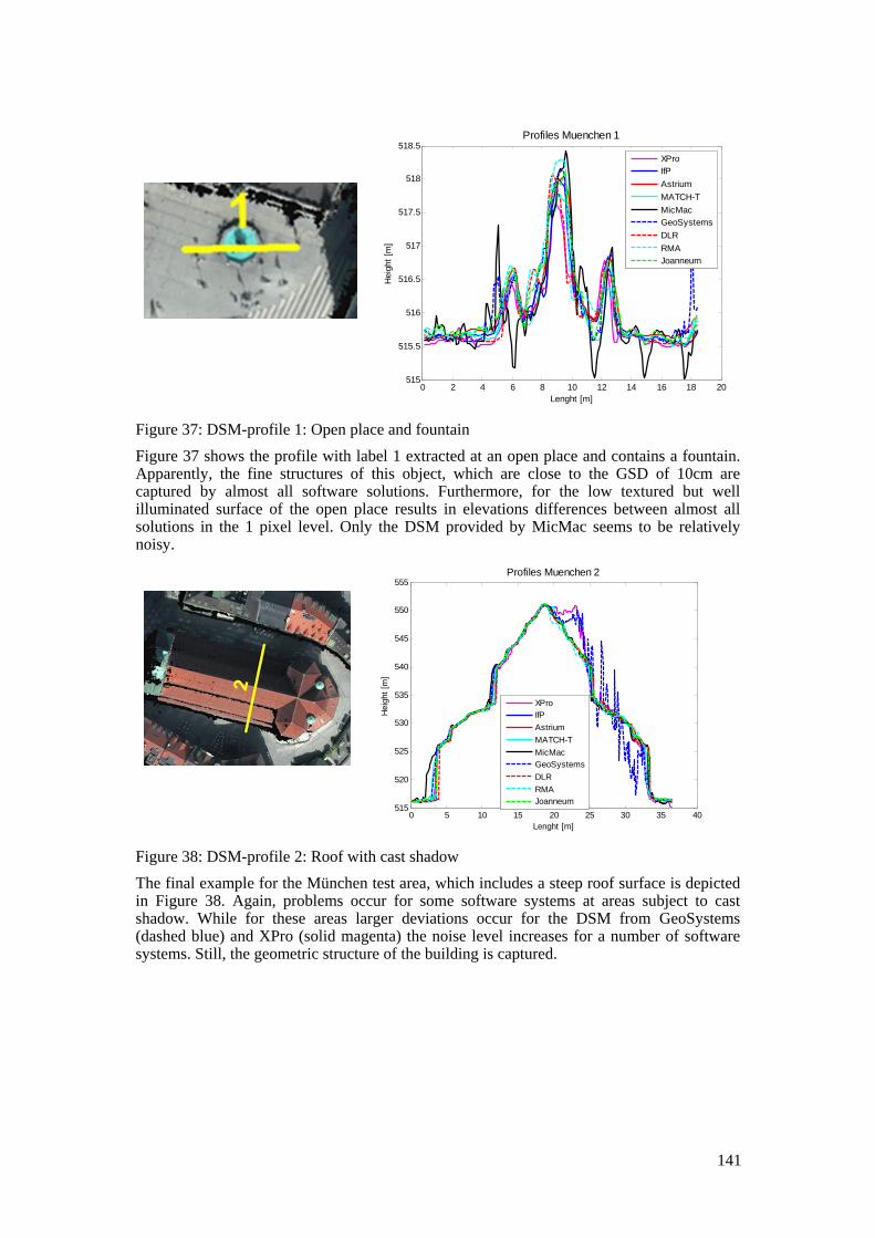
Figure 37: DSM-profile 1: Open place and fountain Figure 37 shows the profile with label 1 extracted at an open place and contains a fountain. Apparently, the fine structures of this object, which are close to the GSD of 10cm are captured by almost all software solutions. Furthermore, for the low textured but well illuminated surface of the open place results in elevations differences between almost all solutions in the 1 pixel level. Only the DSM provided by MicMac seems to be relatively noisy.

0 5 10 15 20 25 30 35 40515

520

525

530

535

540

545

550

555

Lenght [m]

Hei

ght [

m]

Profiles Muenchen 2


Figure 38: DSM-profile 2: Roof with cast shadow The final example for the München test area, which includes a steep roof surface is depicted in Figure 38. Again, problems occur for some software systems at areas subject to cast shadow. While for these areas larger deviations occur for the DSM from GeoSystems (dashed blue) and XPro (solid magenta) the noise level increases for a number of software systems. Still, the geometric structure of the building is captured.

142

5 Conclusions The results presented within the Benchmark on Image Matching clearly demonstrate the potential of software tools for detailed, reliable and accurate photogrammetric 3D data capture from airborne imagery. The aerial image blocks provided a suitable test-bed for software developers to demonstrate the state-of-the-art of their ongoing developments. Furthermore, the accompanying workshop helped potential users like National Mapping and Cadastral agencies (NMCAs) to understand the applicability of such tools for state-wide-generation of high quality DSMs. Obviously, the quality of image based surface reconstruction not only benefits from efficient stereo matching but takes advantage from large image overlaps. The resulting redundancy helps to eliminate erroneous matches and supports the generation of DSM at vertical accuracies close to the sub-pixel level. Most software systems show acceptable run-times even if a standard hardware environment is used. Data sets like the München city area at a size of 1.5kmx1.7km or the semi-rural Vaihingen/Enz area with moderate resolution and overlap at a size of 7.5kmx3.0km can be processed without problems to derive a DSM at grid intervals of 10cm and 20cm, respectively. Still, the benchmark also identified scenarios which can result in difficulties for image based surface reconstruction. DSM differences increased for fine object structures at a size close to the resolution of the available images. Furthermore, cast shadows induced decreasing DSM accuracies for some solutions. Thus, also further development of camera technique to improve the radiometry of the available images would be beneficial. The area covering DSM differences and the extracted profiles helped to indicate the quality of photogrammetric surface reconstruction as available from the respective software systems. Nevertheless, a clear ranking was neither intended nor realized, also due to the fact that software development for image matching is still subject to a considerable momentum. Thus, further improvements can be expected both for matching accuracy and computational performance.

Acknowledgement

Sincere thanks go to my co-members of the project team, Wolfgang Stoessel, State Agency of Surveying and Geoinformation Bavaria, Dr. Michael Gruber, Microsoft Photogrammetry, Prof. Dr. Norbert Pfeifer, Vienna University of Technology, and Michael Franzen, Federal Office for Metrology and Surveying, Vienna. The most important prerequisite for realization of the benchmark on high density image matching for DSM computation is a sufficient number of participants volunteering for data processing. This work is especially acknowledged – without their valuable contribution such an initiative cannot be implemented.

6 References

Cramer, M. (2010): The DGPF-Test on Digital Airborne Camera Evaluation – Overview and Test Design. Photogrammetrie – Fernerkundung – Geoinformation (PFG), Heft 2 (2010), pp. 75-84.

EuroSDR (2012) Proceedings of the 1st EuroSDR workshop on 'High Density Image Matching for DSM Computation'

143

EuroSDR (2013a): http://www.ifp.uni-stuttgart.de/eurosdr/ImageMatching/ web-page of the EuroSDR project Benchmark on Image Matching, last accessed July, 2013.

EuroSDR (2013b) Proceedings of the 2nd EuroSDR workshop on 'High Density Image Matching for DSM Computation' http://geo.tuwien.ac.at/news/2nd-workshop-on-high-density-image-matching-for-dsm-computation-successfully-completed-2013-06-19/.

Fritsch, D., Pfeifer, N. & Franzen, M. (Eds.) (2013): Proceedings of the 2nd EuroSDR workshop on High Density Image Matching for DSM Computation. EuroSDR Publication Series, No. 63.

Haala, N., Hastedt, H., Wolff, K., Ressl, C. & Baltrusch, S. (2010): Digital Photogrammetric Camera Evaluation – Generation of Digital Elevation Models. Photogrammetrie – Fernerkundung – Geoinformation (PFG), Heft 2, pp. 99-115.

Heipke, C. (1993): Performance and state-of-the-art of digital stereo processing. Proceedings of the 44rd Photogrammetric Week, Stuttgart, pp. 173-183.

Hirschmüller, H. (2008): Stereo Processing by Semi-Global Matching and Mutual Information. IEEE Transactions on Pattern Analysis and Machine Intelligence, 30 (2), pp. 328-341.

Scharstein, D. & Szeliski, R. (2002): A Taxonomy and Evaluation of Dense Two-Frame Stereo Correspondence Algorithms. International Journal of Computer Vision, Volume 47, Issue 1-3, April-June 2002, pp. 7-42.

Seitz, S., Curless, B., Diebel, J., Scharstein, D. & Szeliski, R. (2006): A Comparison and Evaluation of Multi-View Stereo Reconstruction Algorithms. IEEE Computer Society Conference on Computer Vision and Pattern Recognition (CVPR'2006).

Szeliski, R. (2010): Computer Vision: Algorithms and Applications. Springer, Chap. 11, Stereo Correspondence.

144

Index Figure Figure 1: Vaihingen/Enz test area with ortho image and DSM............................................118 Figure 2: Vaihingen/Enz: Image overlap (maximum nine-folded) with image footprints and camera stations. The area to be processed is depicted as light blue rectangle ..............118 Figure 3: München test area with DSM (left) and color-coded image overlap (maximum 15 folded) with image footprints, camera stations and area to be processed (right)............119 Figure 4: Visualisation of test area München .......................................................................120 Figure 6: Median DSM for all solutions of the Vaihingen/Enz subsection. .........................124 Figure 7: RMS differences for all solutions for a Vaihingen/Enz subsection. .....................124 Figure 8: Match-T, DSM differences <-2m >2m ......................................................125 Figure 9: Joanneum DSM differences, <-2m >2m....................................................125 Figure 10: IfP Sure DSM differences, <-2m >2m.....................................................126 Figure 11: IGN MicMac DSM differences, <-2m >2m ............................................126 Figure 12: GeoSystems DSM differences, <-2m >2m...............................................127 Figure 13: UltraMap DSM differences, <-2m >2m...................................................127 Figure 14: DLR-SGM DSM differences <-2m >2m .................................................128 Figure 15: Astrium Pixel-Factory, DSM differences <-2m >2m ..............................128 Figure 16: RMA, DSM differences <-2m >2m.........................................................129 Figure 17: SocetSet, DSM differences <-2m >2m ....................................................129 Figure 18: XProSGM, DSM differences <-2m >2m.................................................130 Figure 19: DSM-profile 0: Quarry 1.....................................................................................130 Figure 20: DSM-profile 1: Quarry 2 and vineyard ...............................................................131 Figure 21: DSM-profile 2: Trees ..........................................................................................132 Figure 22: DSM-profile 3: Building and water ....................................................................132 Figure 23: Ortho image of München subsection with profile lines ......................................133 Figure 24: Median DSM for all solutions of the München subsection.................................134 Figure 25: RMS differences for all solutions for München subsection. ...............................134 Figure 26: Match-T, DSM differences <-2m >2m ....................................................135 Figure 27: Joanneum research DSM differences <-2m >2m.....................................135 Figure 28: IfP-SURE DSM differences <-2m >2m...................................................136 Figure 29: IGN MicMac DSM differences <-2m >2m .............................................136 Figure 30: GeoSystems DSM differences <-2m >2m ...............................................137 Figure 31: DLR DSM differences <-2m >2m ...........................................................137

145

Figure 32 Astrium Pixel-Factory differences <-2m >2m ..........................................138 Figure 33: RMA differences <-2m >2m....................................................................138 Figure 34: SocetSet differences <-2m >2m...............................................................139 Figure 35: XProSGM differences <-2m >2m............................................................139 Figure 36: DSM-profile 0: Building and roof structures ......................................................140 Figure 37: DSM-profile 1: Open place and fountain............................................................141 Figure 38: DSM-profile 2: Roof with cast shadow...............................................................141

LIST OF OEEPE/EuroSDR OFFICIAL PUBLICATIONS State – March 2013 1 Trombetti, C.: „Activité de la Commission A de l’OEEPE de 1960 à 1964“ – Cunietti,

M.: „Activité de la Commission B de l’OEEPE pendant la période septembre 1960 – janvier 1964“ – Förstner, R.: „Rapport sur les travaux et les résultats de la Commission C de l’OEEPE (1960–1964)“ – Neumaier, K.: „Rapport de la Commission E pour Lisbonne“ – Weele, A. J. v. d.: „Report of Commission F.“ – Frankfurt a. M. 1964, 50 pages with 7 tables and 9 annexes.

2 Neumaier, K.: „Essais d’interprétation de »Bedford« et de »Waterbury«. Rapport commun établi par les Centres de la Commission E de l’OEEPE ayant participé aux tests“ – „The Interpretation Tests of »Bedford« and »Waterbury«. Common Report Established by all Participating Centres of Commission E of OEEPE“ – „Essais de restitution »Bloc Suisse«. Rapport commun établi par les Centres de la Commission E de l’OEEPE ayant participé aux tests“ – „Test »Schweizer Block«. Joint Report of all Centres of Commission E of OEEPE.“ – Frankfurt a. M. 1966, 60 pages with 44 annexes.

3 Cunietti, M.: „Emploi des blocs de bandes pour la cartographie à grande échelle – Résultats des recherches expérimentales organisées par la Commission B de l’O.E.E.P.E. au cours de la période 1959–1966“ – „Use of Strips Connected to Blocks for Large Scale Mapping – Results of Experimental Research Organized by Commission B of the O.E.E.P.E. from 1959 through 1966.“ – Frankfurt a. M. 1968, 157 pages with 50 figures and 24 tables.

4 Förstner, R.: „Sur la précision de mesures photogrammétriques de coordonnées en terrain montagneux. Rapport sur les résultats de l’essai de Reichenbach de la Commission C de l’OEEPE“ – „The Accuracy of Photogrammetric Co-ordinate Measurements in Mountainous Terrain. Report on the Results of the Reichenbach Test Commission C of the OEEPE.“ – Frankfurt a. M. 1968, Part I: 145 pages with 9 figures; Part II: 23 pages with 65 tables.

5 Trombetti, C.: „Les recherches expérimentales exécutées sur de longues bandes par la Commission A de l’OEEPE.“ – Frankfurt a. M. 1972, 41 pages with 1 figure, 2 tables, 96 annexes and 19 plates.

6 Neumaier, K.: „Essai d’interprétation. Rapports des Centres de la Commission E de l’OEEPE.“ – Frankfurt a. M. 1972, 38 pages with 12 tables and 5 annexes.

7 Wiser, P.: „Etude expérimentale de l’aérotiangulation semi-analytique. Rapport sur l’essai »Gramastetten«.“ – Frankfurt a. M. 1972, 36 pages with 6 figures and 8 tables.

8 „Proceedings of the OEEPE Symposium on Experimental Research on Accuracy of Aerial Triangulation (Results of Oberschwaben Tests)“ Ackermann, F.: „On Statistical Investigation into the Accuracy of Aerial Triangulation. The Test Project Oberschwaben“ – „Recherches statistiques sur la précision de l’aérotriangulation. Le champ d’essai Oberschwaben“– Belzner, H.: „The Planning. Establishing and Flying of the Test Field Oberschwaben“ – Stark, E.: Testblock Oberschwaben, Programme I. Results of Strip Adjustments“ – Ackermann, F.: „Testblock Oberschwaben, Program I. Results of Block-Adjustment by Independent Models“ – Ebner, H.: Comparison of Different Methods of Block Adjustment“ – Wiser, P.: „Propositions pour le traitement des erreurs non-accidentelles“– Camps, F.: „Résultats obtenus dans le cadre du project Oberschwaben 2A“ – Cunietti, M.; Vanossi, A.: „Etude statistique expérimentale des erreurs d’enchaînement des photogrammes“– Kupfer, G.: „Image Geometry as Obtained from Rheidt Test Area Photography“ – Förstner, R.: „The Signal-Field of Baustetten. A Short Report“ – Visser, J.; Leberl, F.; Kure, J.: „OEEPE Oberschwaben Reseau Investigations“ – Bauer, H.: „Compensation of Systematic Errors by Analytical Block Adjustment with Common Image Deformation Parameters.“ – Frankfurt a. M. 1973, 350 pages with 119 figures, 68 tables and 1 annex.

9 Beck, W.: „The Production of Topographic Maps at 1 : 10,000 by Photogrammetric Methods. – With statistical evaluations, reproductions, style sheet and sample fragments by Landesvermessungsamt Baden-Württemberg Stuttgart.“ – Frankfurt a. M. 1976, 89 pages with 10 figures, 20 tables and 20 annexes.

10 „Résultats complémentaires de l’essai d’«Oberriet» of the Commission C de l’OEEPE – Further Results of the Photogrammetric Tests of «Oberriet» of the Commission C of the OEEPE“ Hárry, H.: „Mesure de points de terrain non signalisés dans le champ d’essai d’«Oberriet» – Measurements of Non-Signalized Points in the Test Field «Oberriet» (Abstract)“ – Stickler, A.; Waldhäusl, P.: „Restitution graphique des points et des lignes non signalisés et leur comparaison avec des résultats de mesures sur le terrain dans le champ d’essai d’«Oberriet» – Graphical Plotting of Non-Signalized Points and Lines, and Comparison with Terrestrial Surveys in the Test Field «Oberriet»“ – Förstner, R.: „Résultats complémentaires des transformations de coordonnées de l’essai d’«Oberriet» de la Commission C de l’OEEPE – Further Results from Co-ordinate Transformations of the Test «Oberriet» of Commission C of the OEEPE“ – Schürer, K.: „Comparaison des distances d’«Oberriet» – Comparison of Distances of «Oberriet» (Abstract).“ – Frankfurt a. M. 1975, 158 pages with 22 figures and 26 tables.

11 „25 années de l’OEEPE“ Verlaine, R.: „25 années d’activité de l’OEEPE“ – „25 Years of OEEPE (Summary)“

– Baarda, W.: „Mathematical Models.“ – Frankfurt a. M. 1979, 104 pages with 22 figures.

12 Spiess, E.: „Revision of 1 : 25,000 Topographic Maps by Photogrammetric Methods.“ – Frankfurt a. M. 1985, 228 pages with 102 figures and 30 tables.

13 Timmerman, J.; Roos, P. A.; Schürer, K.; Förstner, R.: On the Accuracy of Photogrammetric Measurements of Buildings – Report on the Results of the Test “Dordrecht”, Carried out by Commission C of the OEEPE. – Frankfurt a. M. 1982, 144 pages with 14 figures and 36 tables.

14 Thompson C. N.: Test of Digitising Methods. – Frankfurt a. M. 1984, 120 pages with 38 figures and 18 tables.

15 Jaakkola, M.; Brindöpke, W.; Kölbl, O.; Noukka, P.: Optimal Emulsions for Large-Scale Mapping – Test of “Steinwedel” – Commission C of the OEEPE 1981–84. – Frankfurt a. M. 1985, 102 pages with 53 figures.

16 Waldhäusl, P.: Results of the Vienna Test of OEEPE Commission C. – Kölbl, O.: Photogrammetric Versus Terrestrial Town Survey. – Frankfurt a. M. 1986, 57 pages with 16 figures, 10 tables and 7 annexes.

17 Commission E of the OEEPE: Influences of Reproduction Techniques on the Identification of Topographic Details on Orthophotomaps. – Frankfurt a. M. 1986, 138 pages with 51 figures, 25 tables and 6 appendices.

18 Förstner, W.: Final Report on the Joint Test on Gross Error Detection of OEEPE and ISP WG III/1. – Frankfurt a. M. 1986, 97 pages with 27 tables and 20 figures.

19 Dowman, I. J.; Ducher, G.: Spacelab Metric Camera Experiment – Test of Image Accuracy. – Frankfurt a. M. 1987, 112 pages with 13 figures, 25 tables and 7 appendices.

20 Eichhorn, G.: Summary of Replies to Questionnaire on Land Information Systems – Commission V – Land Information Systems. – Frankfurt a. M. 1988, 129 pages with 49 tables and 1 annex.

21 Kölbl, O.: Proceedings of the Workshop on Cadastral Renovation – Ecole polytechnique fédérale, Lausanne, 9–11 September, 1987. – Frankfurt a. M. 1988, 337 pages with figures, tables and appendices.

22 Rollin, J.; Dowman, I. J.: Map Compilation and Revision in Developing Areas – Test of Large Format Camera Imagery. – Frankfurt a. M. 1988, 35 pages with 3 figures, 9 tables and 3 appendices.

23 Drummond, J. (ed.): Automatic Digitizing – A Report Submitted by a Working Group of Commission D (Photogrammetry and Cartography). – Frankfurt a. M. 1990, 224 pages with 85 figures, 6 tables and 6 appendices.

24 Ahokas, E.; Jaakkola, J.; Sotkas, P.: Interpretability of SPOT data for General Mapping. – Frankfurt a. M. 1990, 120 pages with 11 figures, 7 tables and 10 appendices.

25 Ducher, G.: Test on Orthophoto and Stereo-Orthophoto Accuracy. – Frankfurt a. M. 1991, 227 pages with 16 figures and 44 tables.

26 Dowman, I. J. (ed.): Test of Triangulation of SPOT Data – Frankfurt a. M. 1991, 206 pages with 67 figures, 52 tables and 3 appendices.

27 Newby, P. R. T.; Thompson, C. N. (ed.): Proceedings of the ISPRS and OEEPE Joint Workshop on Updating Digital Data by Photogrammetric Methods. – Frankfurt a. M. 1992, 278 pages with 79 figures, 10 tables and 2 appendices.

28 Koen, L. A.; Kölbl, O. (ed.): Proceedings of the OEEPE-Workshop on Data Quality in Land Information Systems, Apeldoorn, Netherlands, 4–6 September 1991. – Frankfurt a. M. 1992, 243 pages with 62 figures, 14 tables and 2 appendices.

29 Burman, H.; Torlegård, K.: Empirical Results of GPS – Supported Block Triangulation. – Frankfurt a. M. 1994, 86 pages with 5 figures, 3 tables and 8 appendices.

30 Gray, S. (ed.): Updating of Complex Topographic Databases. – Frankfurt a. M. 1995, 133 pages with 2 figures and 12 appendices.

31 Jaakkola, J.; Sarjakoski, T.: Experimental Test on Digital Aerial Triangulation. – Frankfurt a. M. 1996, 155 pages with 24 figures, 7 tables and 2 appendices.

32 Dowman, I. J.: The OEEPE GEOSAR Test of Geocoding ERS-1 SAR Data. – Frankfurt a. M. 1996, 126 pages with 5 figures, 2 tables and 2 appendices.

33 Kölbl, O.: Proceedings of the OEEPE-Workshop on Application of Digital Photogrammetric Workstations. – Frankfurt a. M. 1996, 453 pages with numerous figures and tables.

34 Blau, E.; Boochs, F.; Schulz, B.-S.: Digital Landscape Model for Europe (DLME). – Frankfurt a. M. 1997, 72 pages with 21 figures, 9 tables, 4 diagrams and 15 appendices.

35 Fuchs, C.; Gülch, E.; Förstner, W.: OEEPE Survey on 3D-City Models. Heipke, C.; Eder, K.: Performance of Tie-Point Extraction in Automatic Aerial

Triangulation. – Frankfurt a. M. 1998, 185 pages with 42 figures, 27 tables and 15 appendices.

36 Kirby, R. P.: Revision Measurement of Large Scale Topographic Data. Höhle, J.: Automatic Orientation of Aerial Images on Database Information. Dequal, S.; Koen, L. A.; Rinaudo, F.: Comparison of National Guidelines for

Technical and Cadastral Mapping in Europe (“Ferrara Test”) – Frankfurt a. M. 1999, 273 pages with 26 figures, 42 tables, 7 special contributions and 9 appendices.

37 Koelbl, O. (ed.): Proceedings of the OEEPE – Workshop on Automation in Digital Photogrammetric Production. – Frankfurt a. M. 1999, 475 pages with numerous figures and tables.

38 Gower, R.: Workshop on National Mapping Agencies and the Internet. Flotron, A.; Koelbl, O.: Precision Terrain Model for Civil Engineering. – Frankfurt a. M. 2000, 140 pages with numerous figures, tables and a CD.

39 Ruas, A.: Automatic Generalisation Project: Learning Process from Interactive Generalisation. – Frankfurt a. M. 2001, 98 pages with 43 figures, 46 tables and 1 appendix.

40 Torlegård, K.; Jonas, N.: OEEPE workshop on Airborne Laserscanning and Interferometric SAR for Detailed Digital Elevation Models. – Frankfurt a. M. 2001, CD: 299 pages with 132 figures, 26 tables, 5 presentations and 2 videos.

41 Radwan, M.; Onchaga, R.; Morales, J.: A Structural Approach to the Management and Optimization of Geoinformation Processes. – Frankfurt a. M. 2001, 174 pages with 74 figures, 63 tables and 1 CD.

42 Heipke, C.; Sester, M.; Willrich, F. (eds.): Joint OEEPE/ISPRS Workshop – From 2D to 3D – Establishment and maintenance of national core geospatial databases. Woodsford, P. (ed.): OEEPE Commission 5 Workshop: Use of XML/GML. – Frankfurt a. M. 2002, CD.

43 Heipke, C.; Jacobsen, K.; Wegmann, H.: Integrated Sensor Orientation – Test Report and Workshop Proceedings. – Frankfurt a. M. 2002, 302 pages with 215 figures, 139 tables and 2 appendices.

44 Holland, D.; Guilford, B.; Murray, K.: Topographic Mapping from High Resolution Space Sensors. – Frankfurt a. M. 2002, 155 pages with numerous figures, tables and 7 appendices.

45 Murray, K. (ed.): OEEPE Workshop on Next Generation Spatial Database – 2005. Altan, M. O.; Tastan, H. (eds.): OEEPE/ISPRS Joint Workshop on Spatial Data Quality Management. 2003, CD.

46 Heipke, C.; Kuittinen, R.; Nagel, G. (eds.): From OEEPE to EuroSDR: 50 years of European Spatial Data Research and beyond – Seminar of Honour. 2003, 103 pages and CD.

47 Woodsford, P.; Kraak, M.; Murray, K.; Chapman, D. (eds.): Visualisation and Rendering – Proceedings EuroSDR Commission 5 Workshop. 2003, CD.

48 Woodsford, P. (ed.): Ontologies & Schema Translation – 2004. Bray, C. (ed.): Positional Accuracy Improvement – 2004. Woodsford, P. (ed.): E-delivery – 2005. Workshops. 2005, CD.

49 Bray, C.; Rönsdorf, C. (eds.): Achieving Geometric Interoperability of Spatial Data, Workshop – 2005. Kolbe, T. H.; Gröger, G. (eds.): International Workshop on Next Generation 3D City Models – 2005. Woodsford, P. (ed.): Workshop on Feature/Object Data Models. 2006, CD.

50 Kaartinen, H.; Hyyppä J.: Evaluation of Building Extraction. Steinnocher, K.; Kressler, F.: Change Detection. Bellmann, A.; Hellwich, O.: Sensor and Data Fusion Contest: Information for Mapping from Airborne SAR and Optical Imagery (Phase I). Mayer, H.; Baltsavias, E.; Bacher, U.: Automated Extraction, Refinement, and Update of Road Databases from Imagery and Other Data. 2006, 280 pages.

51 Höhle, J.; Potuckova J.: The EuroSDR Test “Checking and Improving of Digital Terrain Models”. Skaloud, J.: Reliability of Direct Georeferencing, Phase 1: An Overview of the Current Approaches and Possibilities. Legat, K.; Skaloud, J.; Schmidt, R.: Reliability of Direct Georeferencing, Phase 2: A Case Study on Practical Problems and Solutions. 2006, 184 pages.

52 Murray, K. (ed.): Proceedings of the International Workshop on Land and Marine Information Integration. 2007, CD.

53 Kaartinen, H.; Hyyppä, J.: Tree Extraction. 2008, 56 pages. 54 Patrucco, R.; Murray, K. (eds.): Production Partnership Management Workshop –

2007. Ismael Colomina, I.; Hernández, E. (eds.): International Calibration and Orientation Workshop, EuroCOW 2008. Heipke, C.; Sester, M. (eds.): Geosensor Networks Workshop. Kolbe, T. H. (ed.): Final Report on the EuroSDR CityGML Project. 2008, CD.

55 Cramer, M.: Digital Camera Calibration. 2009, 257 pages. 56 Champion, N.: Detection of Unregistered Buildings for Updating 2D Databases.

Everaerts, J.: NEWPLATFORMS – Unconventional Platforms (Unmanned Aircraft Systems) for Remote Sensing. 2009, 98 pages.

57 Streilein, A.; Kellenberger, T. (eds.): Crowd Sourcing for Updating National Databases. Colomina, I.; Jan Skaloud, J.; Cramer, M. (eds.): International Calibration and Orientation Workshop EuroCOW 2010. Nebiker, S.; Bleisch, S.; Gülch, E.: Final Report on EuroSDR Project Virtual Globes. 2010, CD.

58 Stoter, J.: State-of-the-Art of Automated Generalisation in Commercial Software. Grenzdörffer, G.: Medium Format Cameras. 2010, 266 pages and CD.

59 Rönnholm, P.: Registration Quality – Towards Integration of Laser Scanning and Photogrammetry. Vanden Berghe, I.; Crompvoets, J.; de Vries, W.; Stoter, J.: Atlas of INSPIRE Implementation Methods. 2011, 292 pages and CD.

60 Höhle, J.; Potuckova M.: Assessment of the Qualityof Digital Terrain Models. 2011, 85 pages.

61 Fritsch, D.; Pfeifer, N.; Franzen, M. (eds.): High Density Image Matching for DSM Computation Workshop. 2012, CD.

62 Honkavaara, E.; Markelin, L.; Arbiol, R.; Martínez, L.: Radiometric Aspects of Digital Photogrammetric Images. Kaartinen, H.; Hyyppä, J.; Kukko, A.; Lehtomäki, M.; Jaakkola, A.; Vosselman, G.; Oude Elberink, S.; Rutzinger, M.; Pu, S.; Vaaja, M.: Mobile Mapping - Road Environment Mapping using Mobile Laser Scanning. 2013, 95 pages.

63 Fritsch, D.; Pfeifer, N.; Franzen, M. (eds.): 2nd High Density Image Matching for DSM Computation Workshop. 2013, CD.

The publications can be ordered using the electronic order form of the EuroSDR website www.eurosdr.net

european spatial data research · change detection in high- ... multisource attribute extraction...

Documents