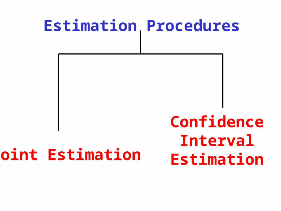
Estimation Procedures

Point Estimation

ConfidenceInterval

Estimation

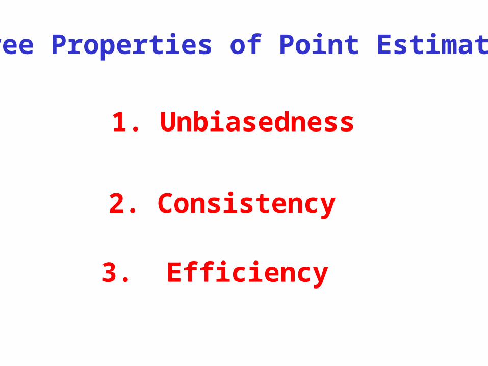
Three Properties of Point Estimators

1. Unbiasedness

2. Consistency

3. Efficiency

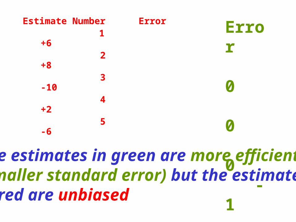
Estimate Number Error 1 +6 2 +8 3 -10 4 +2 5 -6

Error 0 0 0 -1 0

The estimates in green are more efficient(smaller standard error) but the estimatesin red are unbiased

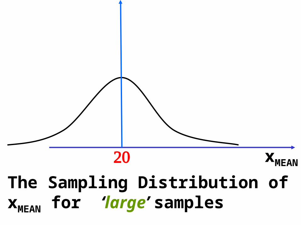
xMEANThe Sampling Distribution ofxMEAN for ‘large’ samples

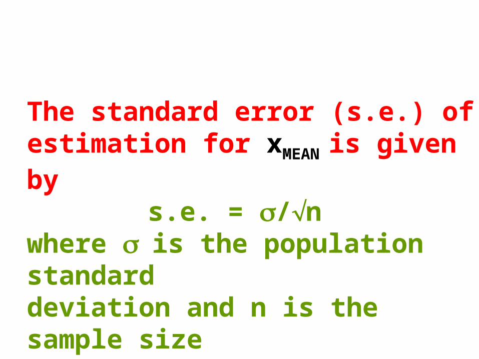
The standard error (s.e.) of estimation for xMEAN is given by

s.e. = /n where is the population standard deviation and n is the sample size

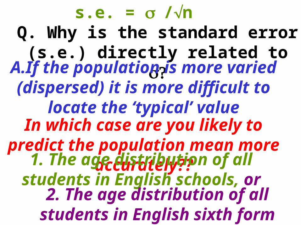
s.e. = /n Q. Why is the standard error (s.e.)

directly related to A.If the population is more varied

(dispersed) it is more difficult to locate the ‘typical’ value

In which case are you likely to predict the population mean more accurately??1. The age distribution of all students in

English schools, or2. The age distribution of all students in

English sixth form colleges?

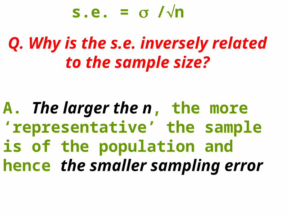
Q. Why is the s.e. inversely related to the sample size?

A. The larger the n, the more ‘representative’ the sample is of the population and hence the smaller sampling error

s.e. = /n

Confidence Interval (CI)Sometimes, it is possible and

convenient to predict, with a certain amount of confidence in the prediction, that the true value of the parameter lies within a specified interval.

Such an interval is called a Confidence Interval (CI)

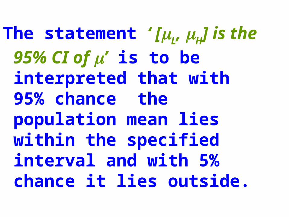
The statement ‘ [L, H] is the 95%

CI of ’ is to be interpreted that with 95% chance the population mean lies within the specified interval and with 5% chance it lies outside.

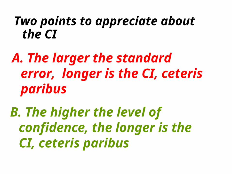
Two points to appreciate about the CI

A. The larger the standard error, longer is the CI, ceteris paribus

B. The higher the level of confidence, the longer is the CI, ceteris paribus

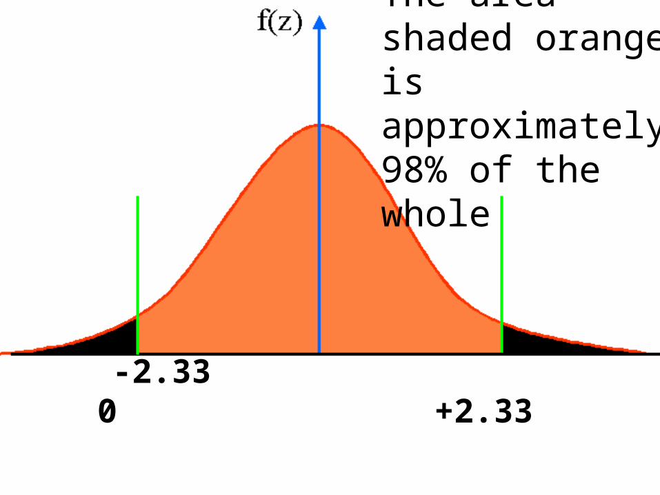
The area shaded orange is approximately98% of the whole

-2.33 0 +2.33

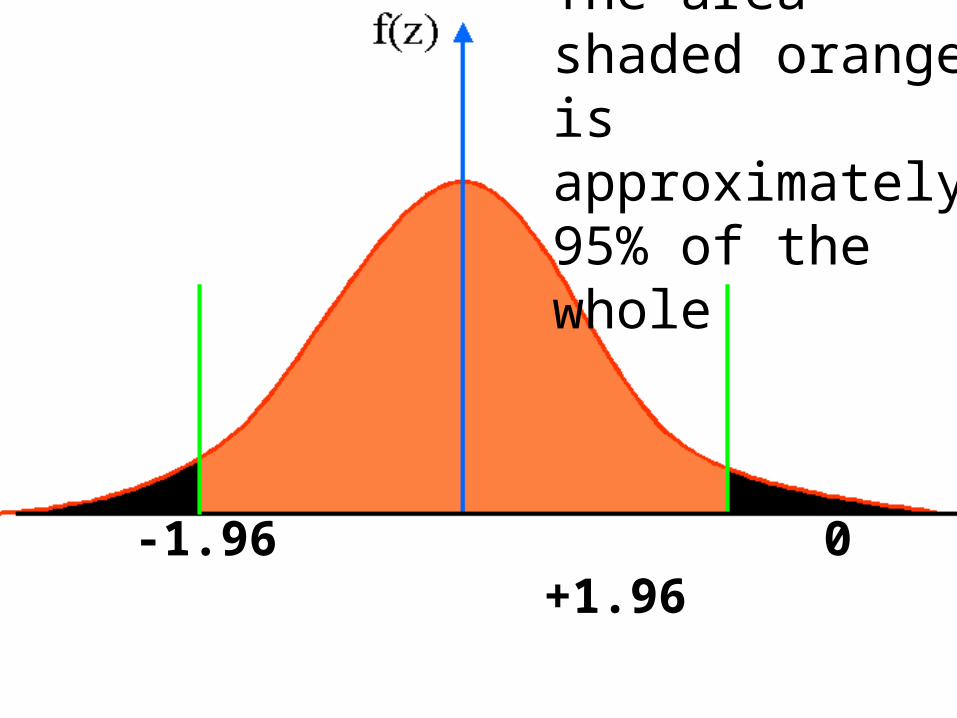
The area shaded orange is approximately95% of the whole

-1.96 0 +1.96

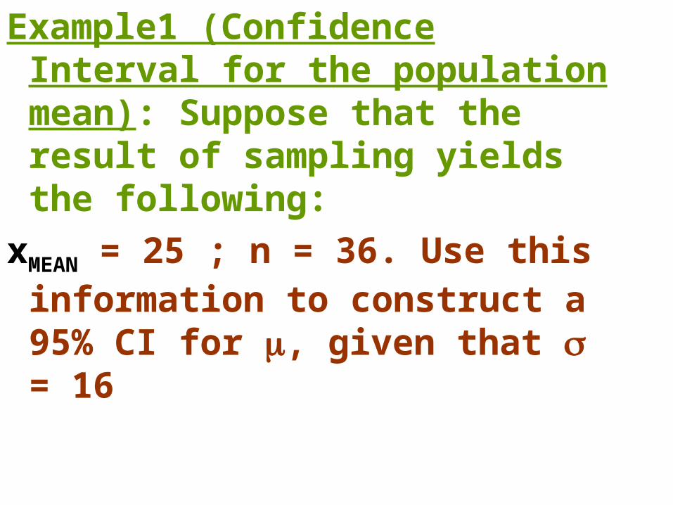
Example1 (Confidence Interval for the population mean): Suppose that the result of sampling yields the following:

xMEAN = 25 ; n = 36. Use this information to construct a 95% CI for , given that = 16

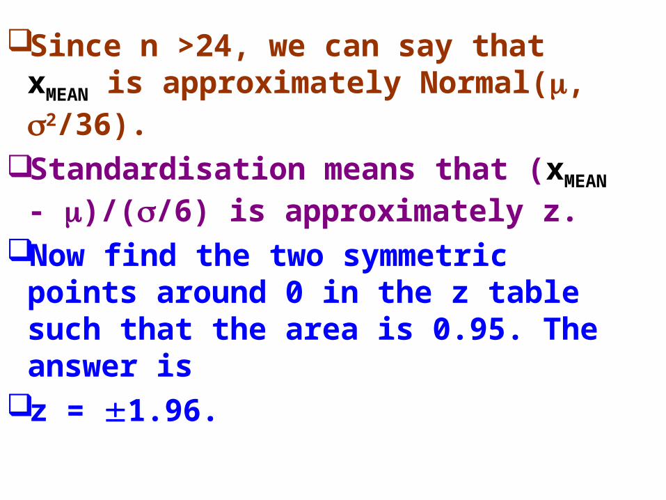
Since n >24, we can say that xMEAN is approximately Normal(, 2/36).

Standardisation means that (xMEAN - )/(/6) is approximately z.

Now find the two symmetric points around 0 in the z table such that the area is 0.95. The answer is

z = 1.96.

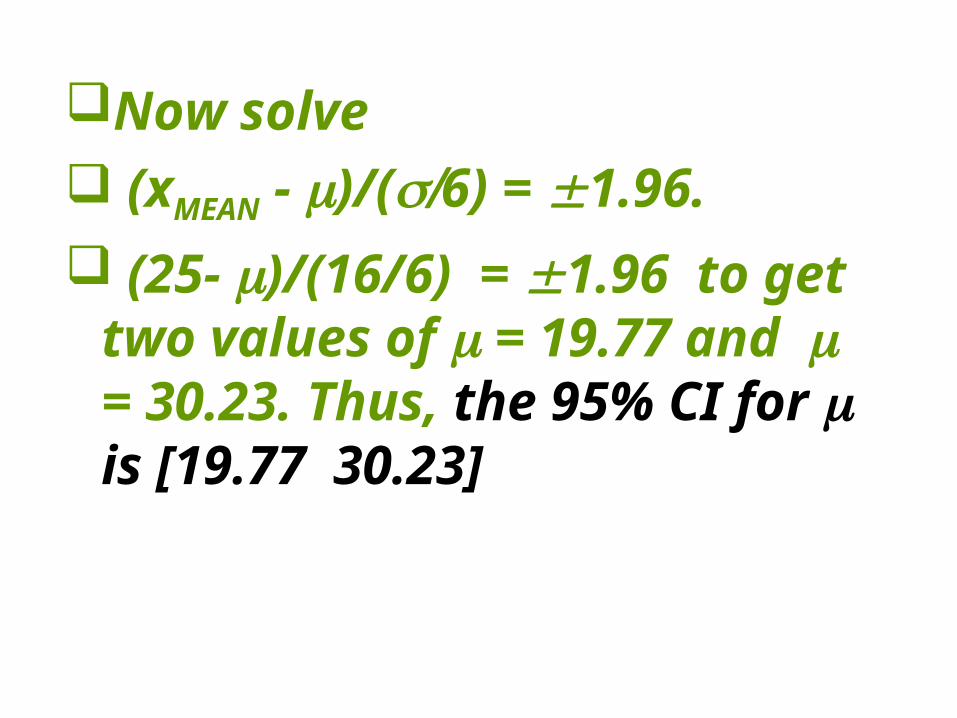
Now solve (xMEAN - )/(6) = 1.96.

 (25- )/(16/6) = 1.96 to get two values of = 19.77 and = 30.23. Thus, the 95% CI for is [19.77 30.23]

Question: How is the length of the CI related to the standard error?

Answer: Ceteris Paribus, the CI is directly related to standard error

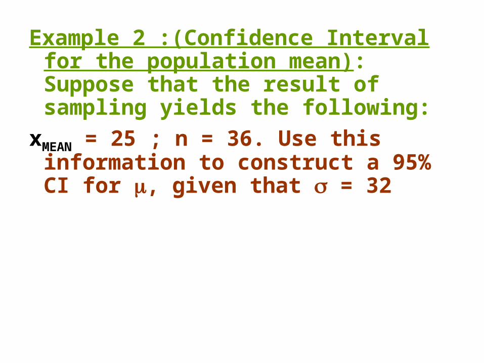
Example 2 :(Confidence Interval for the population mean): Suppose that the result of sampling yields the following:

xMEAN = 25 ; n = 36. Use this information to construct a 95% CI for , given that = 32

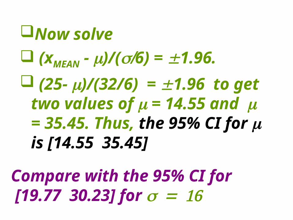
Now solve (xMEAN - )/(6) = 1.96.

 (25- )/(32/6) = 1.96 to get two values of = 14.55 and = 35.45. Thus, the 95% CI for is [14.55 35.45]

Compare with the 95% CI for [19.77 30.23] for

Question: How is the length of the CI related to the level of confidence?

Answer: Ceteris Paribus, the CI will be longer the higher the level of confidence.

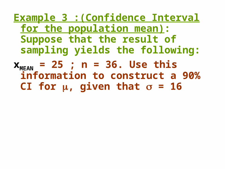
Example 3 :(Confidence Interval for the population mean): Suppose that the result of sampling yields the following:

xMEAN = 25 ; n = 36. Use this information to construct a 90% CI for , given that = 16

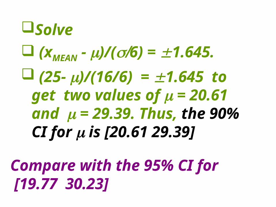
Solve (xMEAN - )/(6) = 1.645.

 (25- )/(16/6) = 1.645 to get two values of = 20.61 and = 29.39. Thus, the 90% CI for is [20.61 29.39]

Compare with the 95% CI for [19.77 30.23]

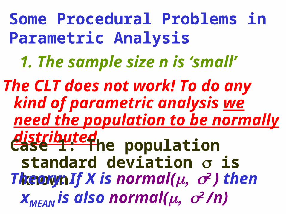
1. The sample size n is ‘small’

The CLT does not work! To do any kind of parametric analysis we need the population to be normally distributed

Case 1: The population standard deviation is known

Theory: If X is normal(2 ) then xMEAN is also normal(2 /n)

Some Procedural Problems inParametric Analysis

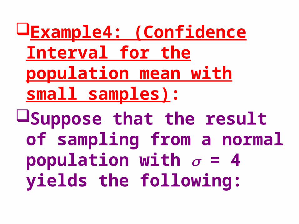
Example4: (Confidence Interval for the population mean with small samples):

Suppose that the result of sampling from a normal population with = 4 yields the following:

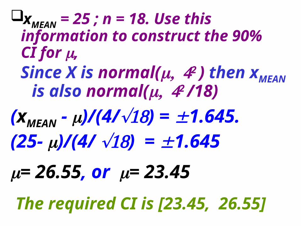
xMEAN = 25 ; n = 18. Use this information to construct the 90% CI for , Since X is normal(2 ) then xMEAN is

also normal(2 /18)

(xMEAN - )/(4/) = 1.645.(25- )/(4/ ) = 1.645

= 26.55, or = 23.45

The required CI is [23.45, 26.55]

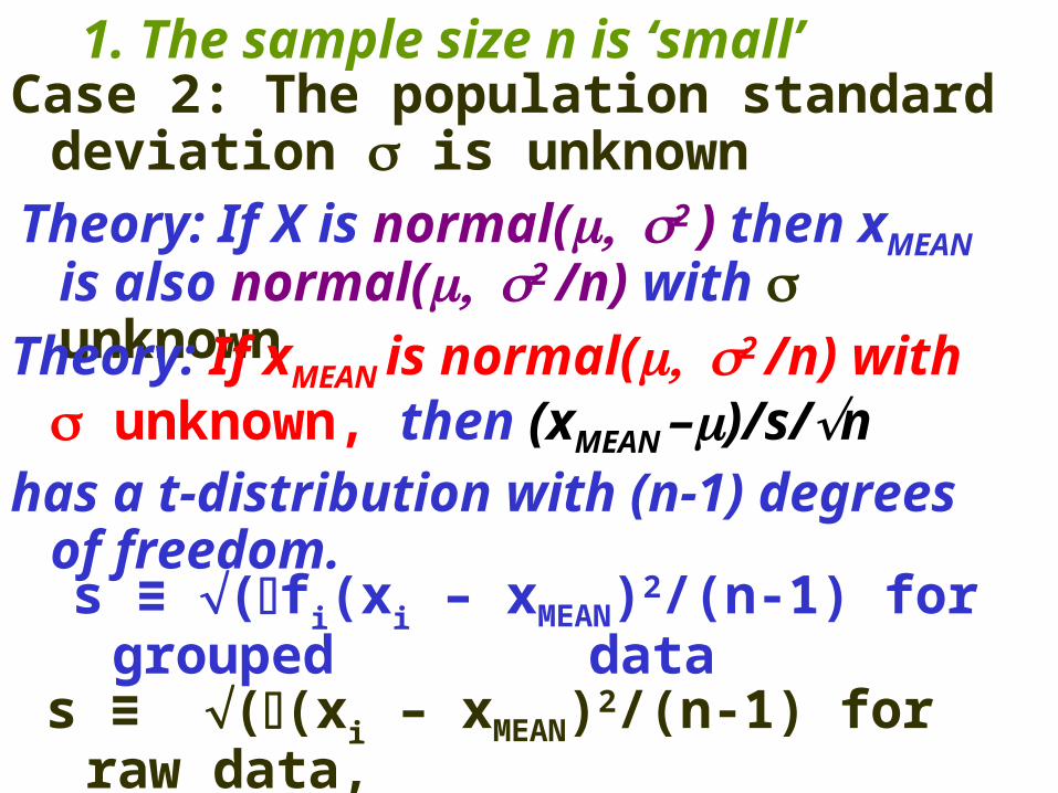
1. The sample size n is ‘small’Case 2: The population standard deviation

is unknownTheory: If X is normal(2 ) then xMEAN is

also normal(2 /n) with unknown

Theory: If xMEAN is normal(2 /n) with unknown, then (xMEAN –)/s/n

has a t-distribution with (n-1) degrees of freedom.

s ≡ ((xi – xMEAN)2/(n-1) for raw data,

s ≡ (fi(xi – xMEAN)2/(n-1) for grouped data

Example5: (Confidence Interval for the population mean):

Suppose that the result of sampling from a normal population yields the following:

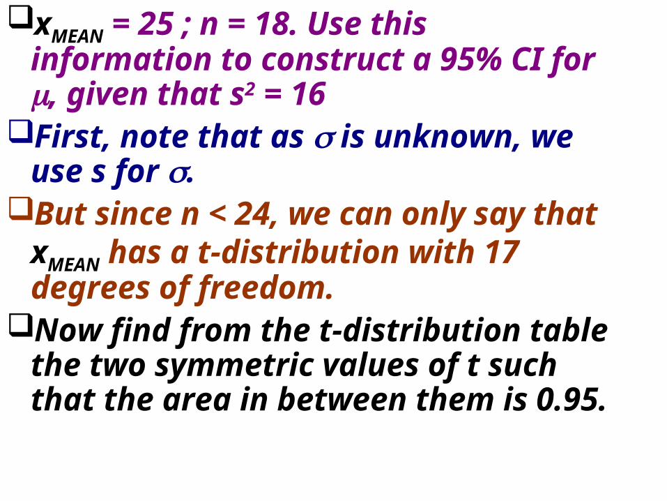
xMEAN = 25 ; n = 18. Use this information to construct a 95% CI for , given that s2 = 16

First, note that as is unknown, we use s for .

But since n < 24, we can only say that xMEAN has a t-distribution with 17 degrees of freedom.

Now find from the t-distribution table the two symmetric values of t such that the area in between them is 0.95.

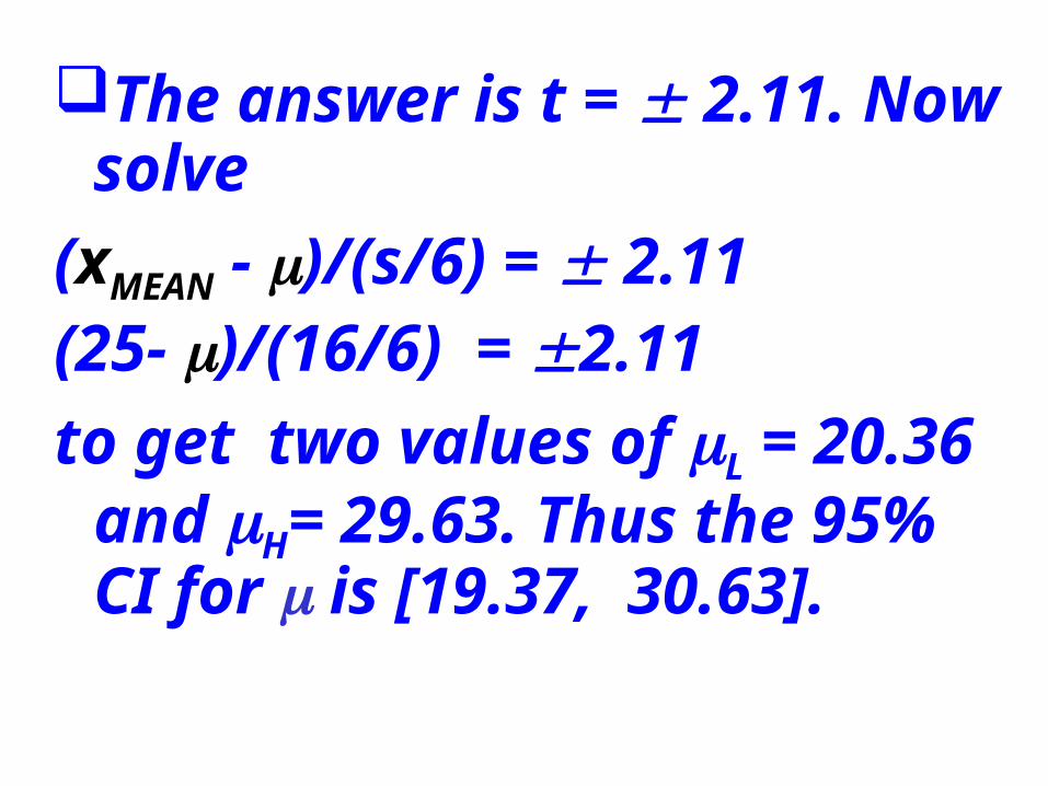
The answer is t = 2.11. Now solve

(xMEAN - )/(s/6) = 2.11(25- )/(16/6) = 2.11

to get two values of L = 20.36 and H= 29.63. Thus the 95% CI for is [19.37, 30.63].

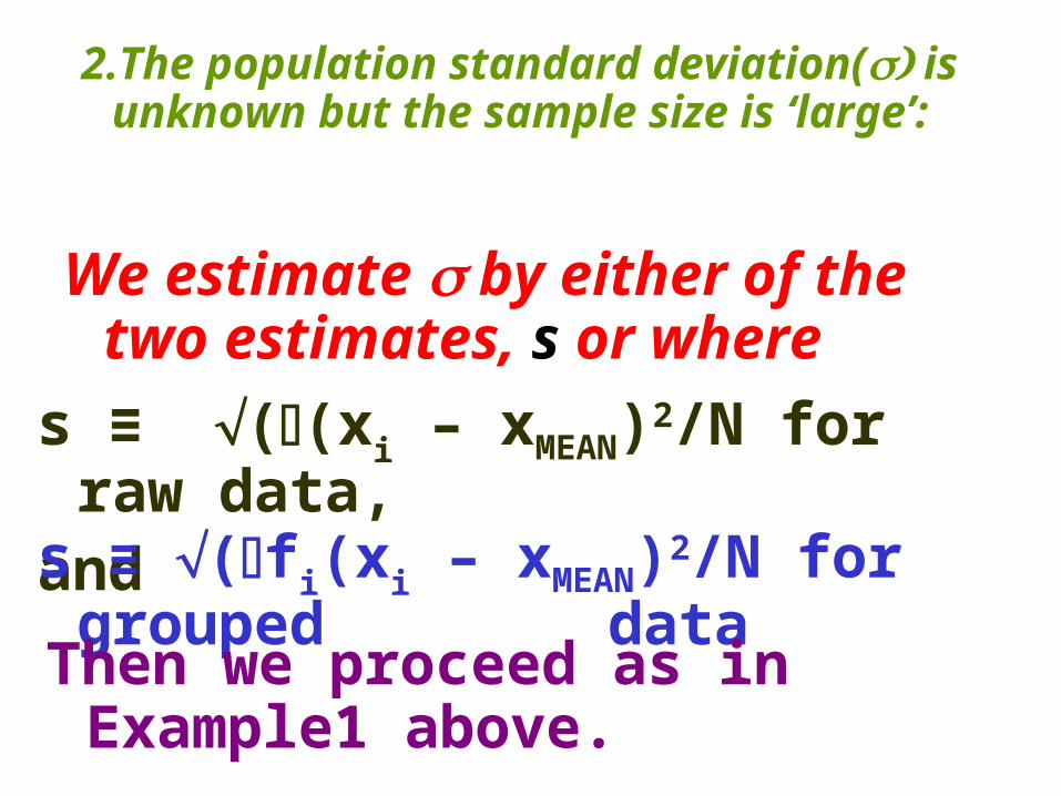
2.The population standard deviation( is unknown but the sample size is ‘large’:

We estimate by either of the two estimates, s or where

s ≡ ((xi – xMEAN)2/N for raw data,

ands ≡ (fi(xi – xMEAN)2/N for grouped

dataThen we proceed as in Example1

above.

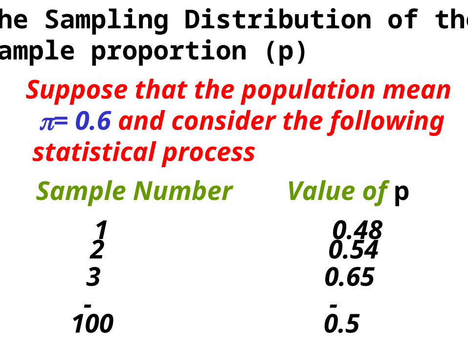
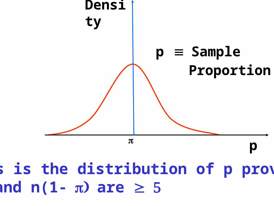
The Sampling Distribution of theSample proportion (p)

Suppose that the population mean = 0.6 and consider the following statistical process

Sample Number Value of p

1 0.48 2 0.54 3 0.65 - -

100 0.5

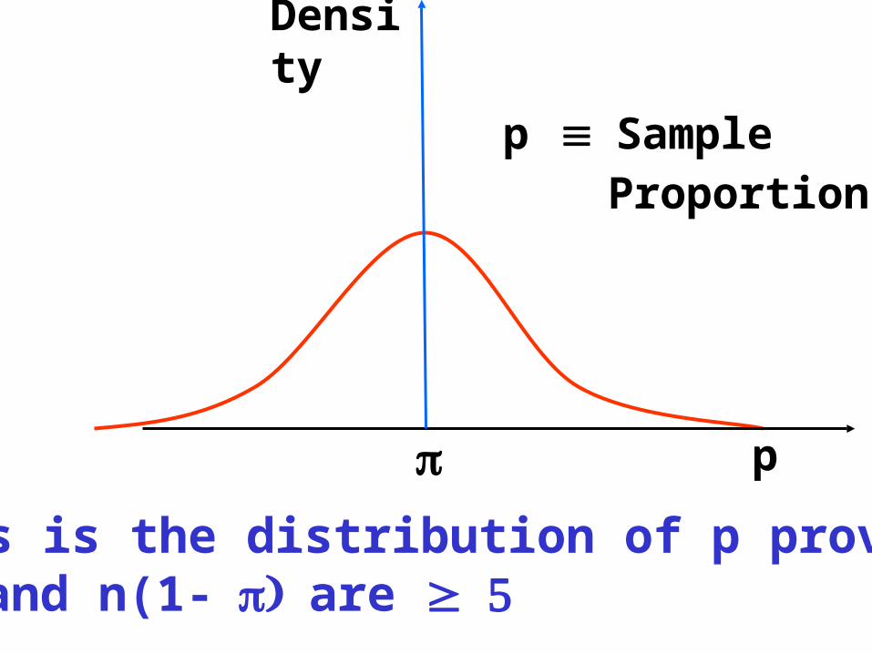
This is the distribution of p providedn and n(1-are

p

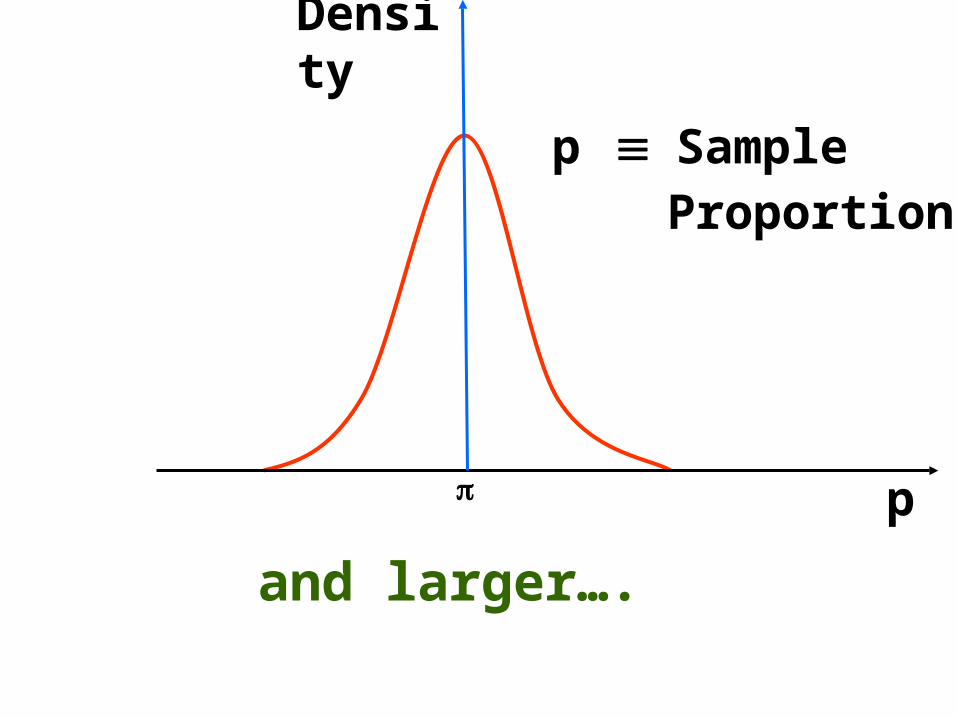
p Sample Proportion

Density

p

Density

p Sample Proportion

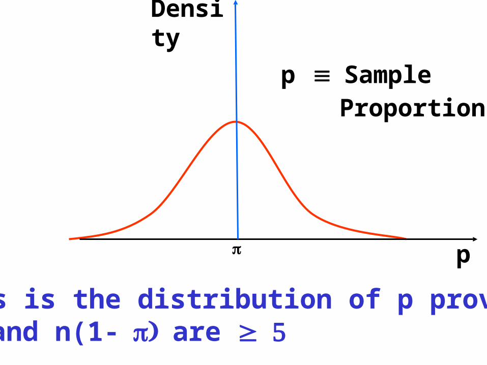
This is the distribution of p providedn and n(1-are

p

Density

p Sample Proportion

This is the distribution of p providedn and n(1-are

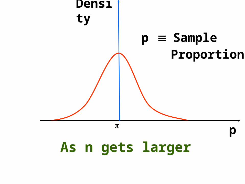
As n gets largerp

Density

p Sample Proportion

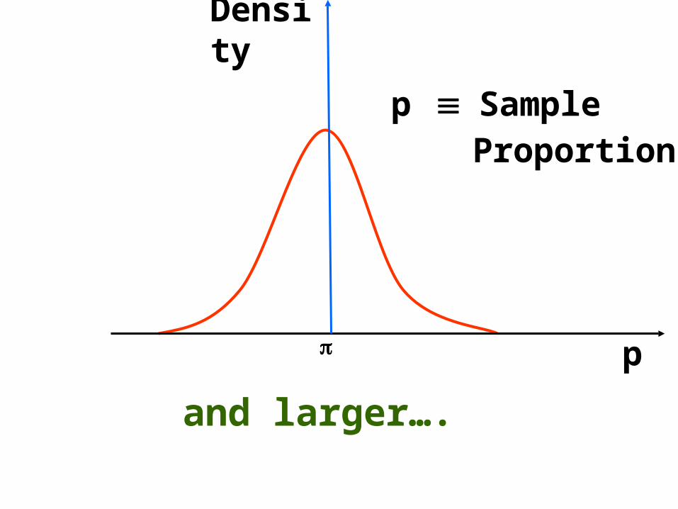
and larger….

p

Density

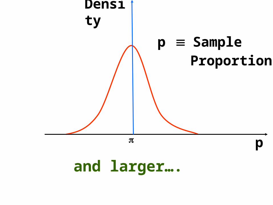
p Sample Proportion

p

Density

and larger….

p Sample Proportion

p

Density

and larger….

p Sample Proportion

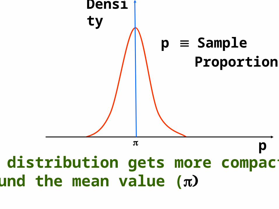
pThe distribution gets more compactaround the mean value (

Density

p Sample Proportion

The distribution gets more compactaround the mean value (

p

Density

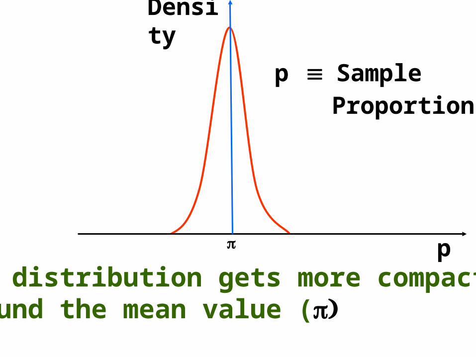
p Sample Proportion

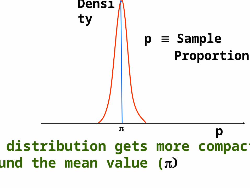
The distribution gets more compactaround the mean value (

p

Density

p Sample Proportion

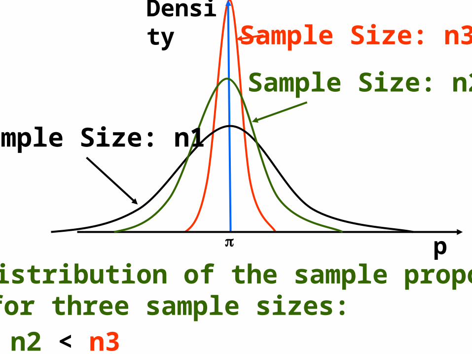
The distribution of the sample proportion(p ) for three sample sizes: n1 < n2 < n3

p

Density

Sample Size: n2

Sample Size: n1

Sample Size: n3

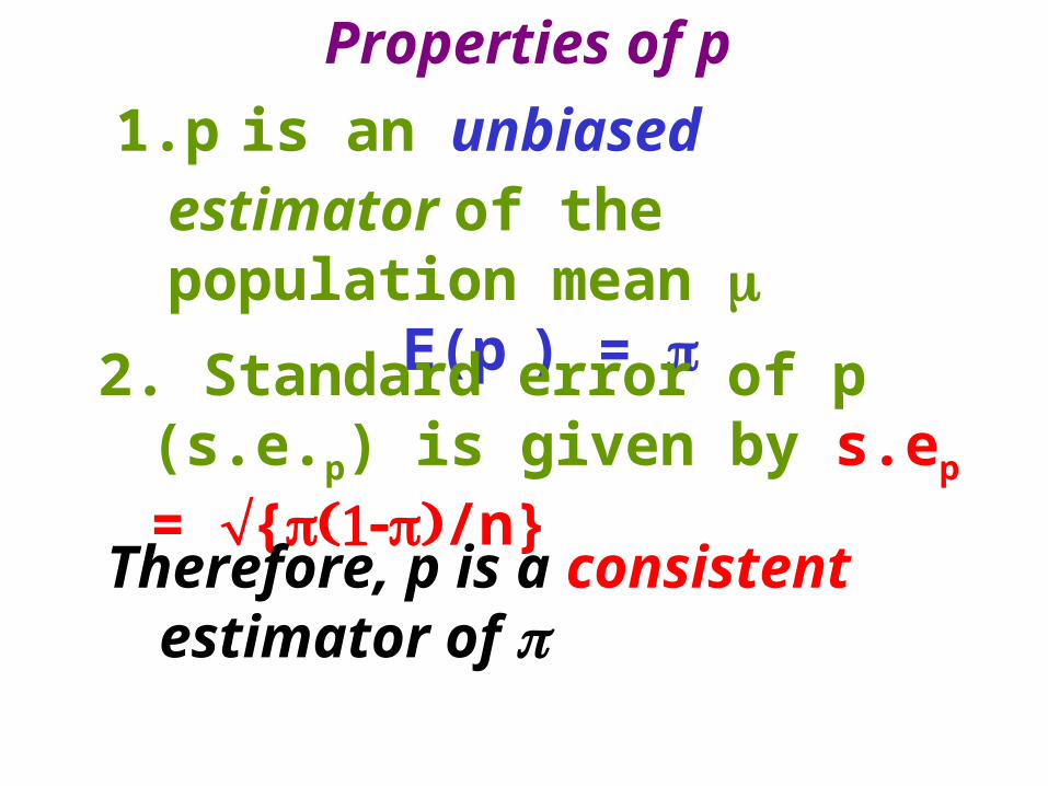
Properties of p

1. p is an unbiased estimator of the population mean

E(p ) =

2. Standard error of p (s.e.p) is given by s.ep = {/n}

Therefore, p is a consistent estimator of

Example1: (Confidence Interval for the population proportion): Suppose that the result of sampling yields the following:

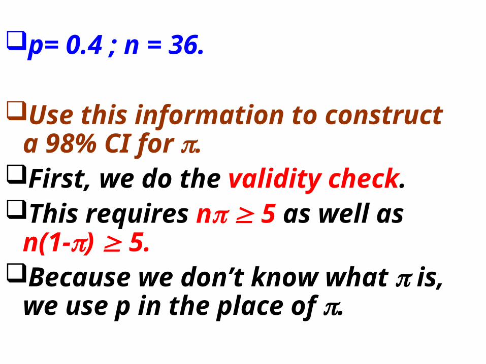
p= 0.4 ; n = 36.

Use this information to construct a 98% CI for .

First, we do the validity check. This requires n 5 as well as n(1-) 5.

Because we don’t know what is, we use p in the place of .

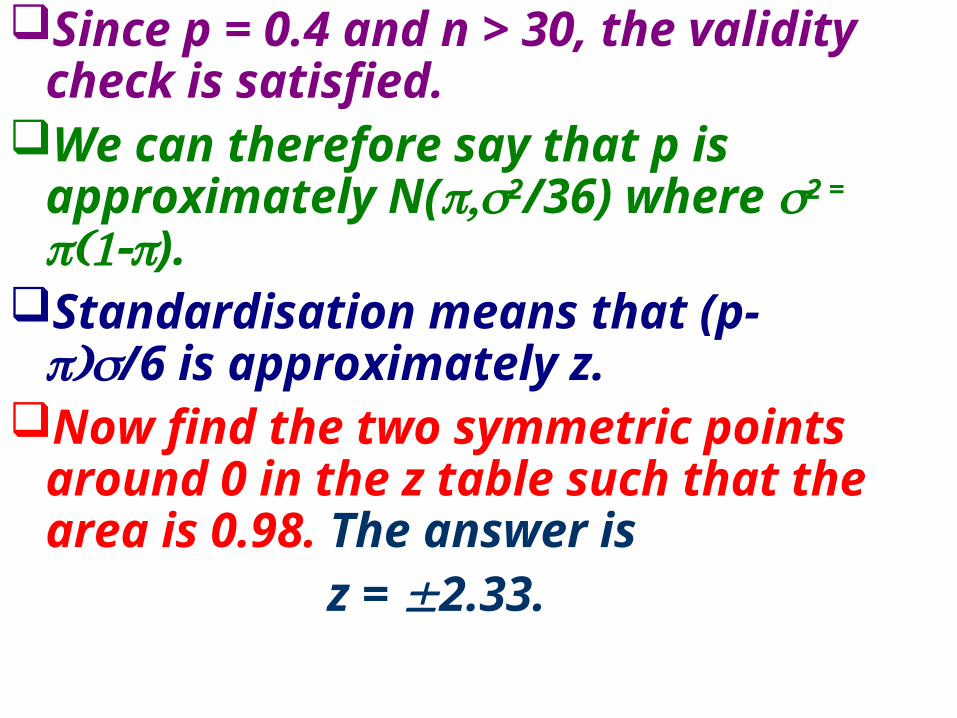
Since p = 0.4 and n > 30, the validity check is satisfied.

We can therefore say that p is approximately N(2/36) where 2 =

).Standardisation means that (p-/6 is

approximately z. Now find the two symmetric points

around 0 in the z table such that the area is 0.98. The answer is

z = 2.33.

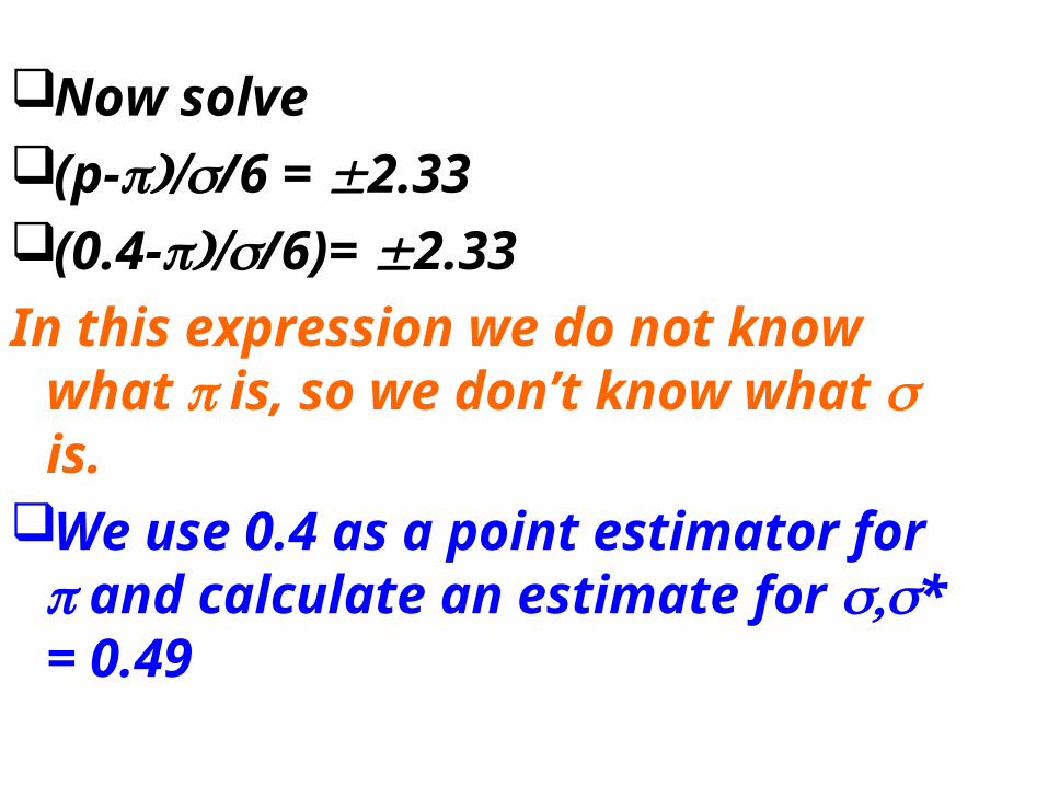
Now solve(p-/6 = 2.33(0.4-/6)= 2.33

In this expression we do not know what is, so we don’t know what is.

We use 0.4 as a point estimator for and calculate an estimate for * = 0.49

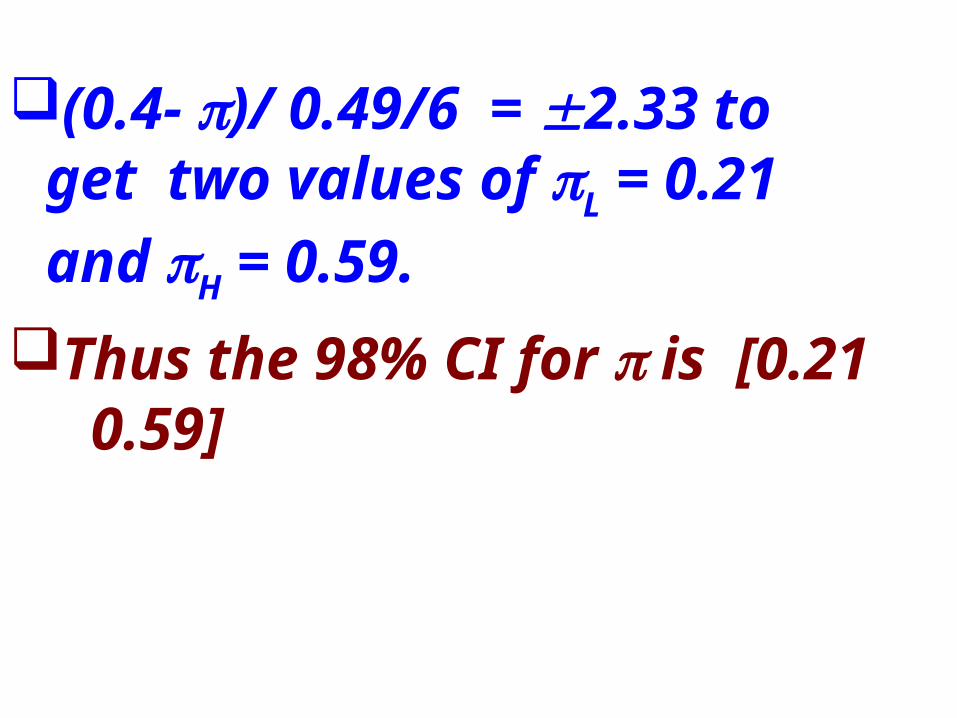
(0.4- )/ 0.49/6 = 2.33 to get two values of L = 0.21 and H =

0.59.Thus the 98% CI for is [0.21

0.59]