estimating musical time information from performed … · estimating musical time information from...

ESTIMATING MUSICAL TIME INFORMATION FROM PERFORMEDMIDI FILES

Harald Grohganz, Michael ClausenBonn University

{grohganz,clausen}@cs.uni-bonn.de

Meinard MullerInternational Audio Laboratories [email protected]

ABSTRACT

Even though originally developed for exchanging control

commands between electronic instruments, MIDI has been

used as quasi standard for encoding and storing score-

related parameters. MIDI allows for representing musi-

cal time information as specified by sheet music as well

as physical time information that reflects performance as-

pects. However, in many of the available MIDI files the

musical beat and tempo information is set to a preset value

with no relation to the actual music content. In this pa-

per, we introduce a procedure to determine the musical

beat grid from a given performed MIDI file. As one main

contribution, we show how the global estimate of the time

signature can be used to correct local errors in the pulse

grid estimation. Different to MIDI quantization, where

one tries to map MIDI note onsets onto a given musical

pulse grid, our goal is to actually estimate such a grid.

In this sense, our procedure can be used in combination

with existing MIDI quantization procedures to convert per-

formed MIDI files into semantically enriched score-like

MIDI files.

1. INTRODUCTION

MIDI (Music Instrument Digital Interface) is used as a

standard protocol for controlling and synchronizing elec-

tronic instruments and synthesizers [10]. Even though

MIDI has not originally been developed to be used as a

symbolic music format and imposes many limitation of

what can be actually represented [11, 13], the importance

of MIDI results from its widespread usage over the last

three decades and the abundance of MIDI data freely avail-

able on the web. An important feature of the MIDI for-

mat is that it can handle musical as well as physical on-

set times and note durations. In particular, the header of

a MIDI file specifies the number of basic time units (re-

ferred to as ticks) per quarter note. Physical timing is then

given by means of additional tempo messages that deter-

mine the number of microseconds per quarter note. On the

one hand, disregarding the tempo messages makes it pos-

c© Harald Grohganz, Michael Clausen, Meinard Muller.

Licensed under a Creative Commons Attribution 4.0 International Li-

cense (CC BY 4.0). Attribution: Harald Grohganz, Michael Clausen,

Meinard Muller. “Estimating Musical Time Information from Performed

MIDI Files”, 15th International Society for Music Information Retrieval

Conference, 2014.

(a)

(b)

(c)

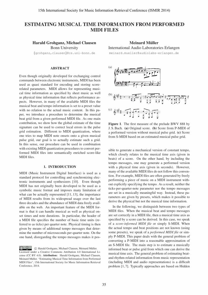
Figure 1. The first measure of the prelude BWV 888 by

J. S. Bach. (a) Original score. (b) Score from P-MIDI of

a performed version without musical pulse grid. (c) Score

from S-MIDI based on an estimated musical pulse grid.

sible to generate a mechanical version of constant tempo,

which closely relates to the musical time axis (given in

beats) of a score. On the other hand, by including the

tempo messages, one may generate a performed version

with a physical time axis (given in seconds). However,

many of the available MIDI files do not follow this conven-

tion. For example, MIDI files are often generated by freely

performing a piece of music on a MIDI instrument with-

out explicitly specifying the tempo. As a result, neither the

ticks-per-quarter-note parameter nor the tempo messages

are set in a musically meaningful way. Instead, these pa-

rameters are given by presets, which makes it possible to

derive the physical but not the musical time information.

In the following, we distinguish between two types of

MIDI files. When the musical beat and tempo messages

are set correctly in a MIDI file, then a musical time axis as

specified by a score can be derived. In this case, we speak

of a score-informed MIDI file or simply S-MIDI. When

the actual tempo and beat positions are not known (using

some presets), we speak of a performed MIDI file or sim-

ply P-MIDI. This paper deals with the general problem of

converting a P-MIDI into a reasonable approximation of

an S-MIDI file. The main step is to estimate a musically

informed beat or pulse grid from which one can derive the

musical time axis. The general problem of estimating beat-

and rhythm-related information from music representation

(including MIDI and audio representations) is a difficult

problem [1, 7]. Typically approaches are based on Hidden

15th International Society for Music Information Retrieval Conference (ISMIR 2014)

35

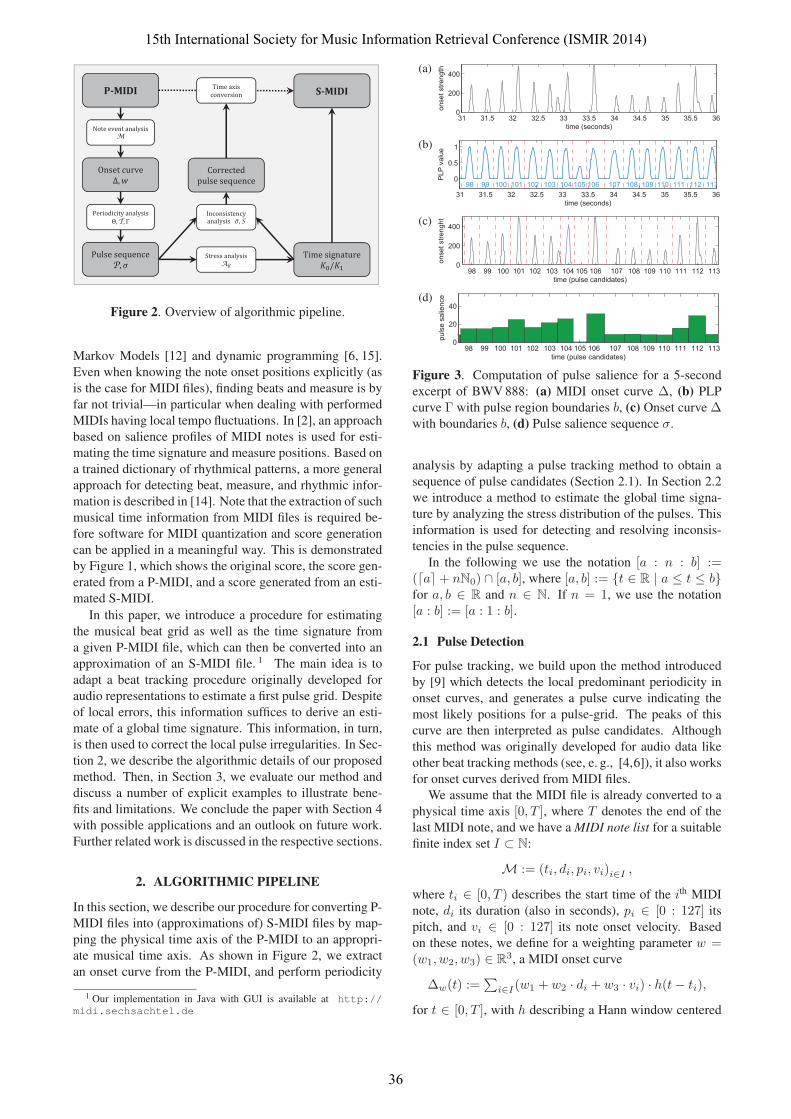
P MIDI S MIDI

P

T

M

A

S

Figure 2. Overview of algorithmic pipeline.

Markov Models [12] and dynamic programming [6, 15].

Even when knowing the note onset positions explicitly (as

is the case for MIDI files), finding beats and measure is by

far not trivial—in particular when dealing with performed

MIDIs having local tempo fluctuations. In [2], an approach

based on salience profiles of MIDI notes is used for esti-

mating the time signature and measure positions. Based on

a trained dictionary of rhythmical patterns, a more general

approach for detecting beat, measure, and rhythmic infor-

mation is described in [14]. Note that the extraction of such

musical time information from MIDI files is required be-

fore software for MIDI quantization and score generation

can be applied in a meaningful way. This is demonstrated

by Figure 1, which shows the original score, the score gen-

erated from a P-MIDI, and a score generated from an esti-

mated S-MIDI.

In this paper, we introduce a procedure for estimating

the musical beat grid as well as the time signature from

a given P-MIDI file, which can then be converted into an

approximation of an S-MIDI file. 1 The main idea is to

adapt a beat tracking procedure originally developed for

audio representations to estimate a first pulse grid. Despite

of local errors, this information suffices to derive an esti-

mate of a global time signature. This information, in turn,

is then used to correct the local pulse irregularities. In Sec-

tion 2, we describe the algorithmic details of our proposed

method. Then, in Section 3, we evaluate our method and

discuss a number of explicit examples to illustrate bene-

fits and limitations. We conclude the paper with Section 4

with possible applications and an outlook on future work.

Further related work is discussed in the respective sections.

2. ALGORITHMIC PIPELINE

In this section, we describe our procedure for converting P-

MIDI files into (approximations of) S-MIDI files by map-

ping the physical time axis of the P-MIDI to an appropri-

ate musical time axis. As shown in Figure 2, we extract

an onset curve from the P-MIDI, and perform periodicity

1 Our implementation in Java with GUI is available at http://midi.sechsachtel.de

(a)

31 31.5 32 32.5 33 33.5 34 34.5 35 35.5 360

200

400

time (seconds)

onse

t stre

ngth

(b)

31 31.5 32 32.5 33 33.5 34 34.5 35 35.5 36

0

0.5

1

time (seconds)

PLP

val

ue

98 99 100 101 102 103 104 105 106 107 108 109 110 111 112 113

(c)

98 99 100 101 102 103 104 105 106 107 108 109 110 111 112 1130

200

400

time (pulse candidates)

onse

t stre

nght

(d)

98 99 100 101 102 103 104 105 106 107 108 109 110 111 112 1130

20

40

time (pulse candidates)

puls

e sa

lienc

e

Figure 3. Computation of pulse salience for a 5-second

excerpt of BWV 888: (a) MIDI onset curve Δ, (b) PLP

curve Γ with pulse region boundaries b, (c) Onset curve Δwith boundaries b, (d) Pulse salience sequence σ.

analysis by adapting a pulse tracking method to obtain a

sequence of pulse candidates (Section 2.1). In Section 2.2

we introduce a method to estimate the global time signa-

ture by analyzing the stress distribution of the pulses. This

information is used for detecting and resolving inconsis-

tencies in the pulse sequence.

In the following we use the notation [a : n : b] :=(�a�+ nN0) ∩ [a, b], where [a, b] := {t ∈ R | a ≤ t ≤ b}for a, b ∈ R and n ∈ N. If n = 1, we use the notation

[a : b] := [a : 1 : b].

2.1 Pulse Detection

For pulse tracking, we build upon the method introduced

by [9] which detects the local predominant periodicity in

onset curves, and generates a pulse curve indicating the

most likely positions for a pulse-grid. The peaks of this

curve are then interpreted as pulse candidates. Although

this method was originally developed for audio data like

other beat tracking methods (see, e. g., [4,6]), it also works

for onset curves derived from MIDI files.

We assume that the MIDI file is already converted to a

physical time axis [0, T ], where T denotes the end of the

last MIDI note, and we have a MIDI note list for a suitable

finite index set I ⊂ N:

M := (ti, di, pi, vi)i∈I ,

where ti ∈ [0, T ) describes the start time of the ith MIDI

note, di its duration (also in seconds), pi ∈ [0 : 127] its

pitch, and vi ∈ [0 : 127] its note onset velocity. Based

on these notes, we define for a weighting parameter w =(w1, w2, w3) ∈ R

3, a MIDI onset curve

Δw(t) :=∑

i∈I(w1 + w2 · di + w3 · vi) · h(t− ti),

for t ∈ [0, T ], with h describing a Hann window centered


36

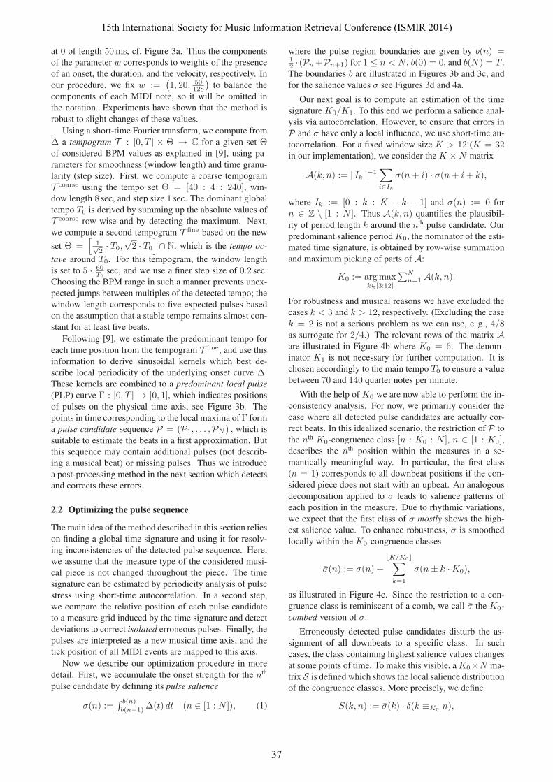
at 0 of length 50ms, cf. Figure 3a. Thus the components

of the parameter w corresponds to weights of the presence

of an onset, the duration, and the velocity, respectively. In

our procedure, we fix w :=(1, 20, 50

128

)to balance the

components of each MIDI note, so it will be omitted in

the notation. Experiments have shown that the method is

robust to slight changes of these values.

Using a short-time Fourier transform, we compute from

Δ a tempogram T : [0, T ] × Θ → C for a given set Θof considered BPM values as explained in [9], using pa-

rameters for smoothness (window length) and time granu-

larity (step size). First, we compute a coarse tempogram

T coarse using the tempo set Θ = [40 : 4 : 240], win-

dow length 8 sec, and step size 1 sec. The dominant global

tempo T0 is derived by summing up the absolute values of

T coarse row-wise and by detecting the maximum. Next,

we compute a second tempogram T fine based on the new

set Θ =[

1√2· T0,

√2 · T0

]∩ N, which is the tempo oc-

tave around T0. For this tempogram, the window length

is set to 5 · 60T0

sec, and we use a finer step size of 0.2 sec.

Choosing the BPM range in such a manner prevents unex-

pected jumps between multiples of the detected tempo; the

window length corresponds to five expected pulses based

on the assumption that a stable tempo remains almost con-

stant for at least five beats.

Following [9], we estimate the predominant tempo for

each time position from the tempogram T fine, and use this

information to derive sinusoidal kernels which best de-

scribe local periodicity of the underlying onset curve Δ.

These kernels are combined to a predominant local pulse(PLP) curve Γ : [0, T ] → [0, 1], which indicates positions

of pulses on the physical time axis, see Figure 3b. The

points in time corresponding to the local maxima of Γ form

a pulse candidate sequence P = (P1, . . . ,PN ) , which is

suitable to estimate the beats in a first approximation. But

this sequence may contain additional pulses (not describ-

ing a musical beat) or missing pulses. Thus we introduce

a post-processing method in the next section which detects

and corrects these errors.

2.2 Optimizing the pulse sequence

The main idea of the method described in this section relies

on finding a global time signature and using it for resolv-

ing inconsistencies of the detected pulse sequence. Here,

we assume that the measure type of the considered musi-

cal piece is not changed throughout the piece. The time

signature can be estimated by periodicity analysis of pulse

stress using short-time autocorrelation. In a second step,

we compare the relative position of each pulse candidate

to a measure grid induced by the time signature and detect

deviations to correct isolated erroneous pulses. Finally, the

pulses are interpreted as a new musical time axis, and the

tick position of all MIDI events are mapped to this axis.

Now we describe our optimization procedure in more

detail. First, we accumulate the onset strength for the nth

pulse candidate by defining its pulse salience

σ(n) :=∫ b(n)

b(n−1)Δ(t) dt (n ∈ [1 : N ]), (1)

where the pulse region boundaries are given by b(n) =12 · (Pn+Pn+1) for 1 ≤ n < N , b(0) = 0, and b(N) = T .

The boundaries b are illustrated in Figures 3b and 3c, and

for the salience values σ see Figures 3d and 4a.

Our next goal is to compute an estimation of the time

signature K0/K1. To this end we perform a salience anal-

ysis via autocorrelation. However, to ensure that errors in

P and σ have only a local influence, we use short-time au-

tocorrelation. For a fixed window size K > 12 (K = 32in our implementation), we consider the K ×N matrix

A(k, n) := | Ik |−1∑i∈Ik

σ(n+ i) · σ(n+ i+ k),

where Ik := [0 : k : K − k − 1] and σ(n) := 0 for

n ∈ Z \ [1 : N ]. Thus A(k, n) quantifies the plausibil-

ity of period length k around the nth pulse candidate. Our

predominant salience period K0, the nominator of the esti-

mated time signature, is obtained by row-wise summation

and maximum picking of parts of A:

K0 := argmaxk∈[3:12]

∑Nn=1 A(k, n).

For robustness and musical reasons we have excluded the

cases k < 3 and k > 12, respectively. (Excluding the case

k = 2 is not a serious problem as we can use, e. g., 4/8as surrogate for 2/4.) The relevant rows of the matrix Aare illustrated in Figure 4b where K0 = 6. The denom-

inator K1 is not necessary for further computation. It is

chosen accordingly to the main tempo T0 to ensure a value

between 70 and 140 quarter notes per minute.

With the help of K0 we are now able to perform the in-

consistency analysis. For now, we primarily consider the

case where all detected pulse candidates are actually cor-

rect beats. In this idealized scenario, the restriction of P to

the nth K0-congruence class [n : K0 : N ], n ∈ [1 : K0],describes the nth position within the measures in a se-

mantically meaningful way. In particular, the first class

(n = 1) corresponds to all downbeat positions if the con-

sidered piece does not start with an upbeat. An analogous

decomposition applied to σ leads to salience patterns of

each position in the measure. Due to rhythmic variations,

we expect that the first class of σ mostly shows the high-

est salience value. To enhance robustness, σ is smoothed

locally within the K0-congruence classes

σ(n) := σ(n) +

�K/K0�∑k=1

σ(n± k ·K0),

as illustrated in Figure 4c. Since the restriction to a con-

gruence class is reminiscent of a comb, we call σ the K0-combed version of σ.

Erroneously detected pulse candidates disturb the as-

signment of all downbeats to a specific class. In such

cases, the class containing highest salience values changes

at some points of time. To make this visible, a K0×N ma-

trix S is defined which shows the local salience distribution

of the congruence classes. More precisely, we define

S(k, n) := σ(k) · δ(k ≡K0 n),


37

(a)

50 100 150 200 250 300 350 4000

10

20

30

40

50

pulse candidates

puls

e sa

lienc

e

(b)

puls

e pe

riodi

city

pulse candidates50 100 150 200 250 300 350 400

2

4

6

8

10

12

0

0.2

0.4

0.6

0.8

1

(c)

50 100 150 200 250 300 35050

100

150

200

250

pulse candidates

smoo

thed

pul

se s

alie

nce (d)

50 100 150 200 250 300 350 40050

100

150

200

250

pulse candidates

smoo

thed

pul

se s

alie

nce

(e)

beat

con

grue

nce

clas

s


1

2

3

4

5

6

0

0.2

0.4

0.6

0.8

1 (f)

beat

con

grue

nce

clas

s


1

2

3

4

5

6

0

0.2

0.4

0.6

0.8

1

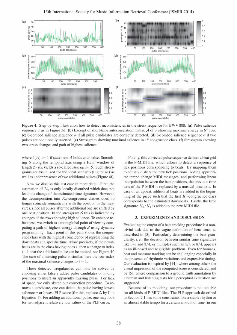
Figure 4. Step-by-step illustration how to detect inconsistencies in the stress sequence for BWV 888: (a) Pulse salience

sequence σ as in Figure 3d. (b) Excerpt of short-time autocorrelation matrix A of σ showing maximal energy in 6th row.

(c) 6-combed salience sequence σ if all pulse candidates are correctly detected. (d) 6-combed salience sequence σ if two

pulses are additionally inserted. (e) Stressgram showing maximal salience in 1st congruence class. (f) Stressgram showing

two stress changes and path of highest salience.

where δ(A) := 1 if statement A holds and 0 else. Smooth-

ing S along the temporal axis using a Hann window of

length 2 ·K0 yields a so-called stressgram S. Such stress-

grams are visualized for the ideal scenario (Figure 4e) as

well as under presence of two additional pulses (Figure 4f).

Now we discuss this last case in more detail. First, the

estimation of K0 is only locally disturbed which does not

lead to a change of the estimated time signature. However,

the decomposition into K0-congruence classes does no

longer coincide semantically with the position in the mea-

sures, since all pulses after the additional one are shifted by

one beat position. In the stressgram S this is indicated by

changes of the rows showing high salience. To enhance ro-

bustness, we switch to a more global point of view by com-

puting a path of highest energy through S using dynamic

programming. Each point in this path shows the congru-

ence class with the highest coincidence of representing the

downbeats at a specific time. More precisely, if the down-

beats are in the class having index i, then a change to index

i+1 near the additional pulse can be noticed, see Figure 4f.

The case of a missing pulse is similar, here the row index

of the maximal salience changes to i− 1.

These detected irregularities can now be solved by

choosing either falsely added pulse candidates or finding

positions to insert an apparently missing pulse. For lack

of space, we only sketch our correction procedure. To re-

move a candidate, one can delete the pulse having lowest

salience σ or lowest PLP score (for this, replace Δ by Γ in

Equation 1). For adding an additional pulse, one may look

for two adjacent relatively low values of the PLP curve.

Finally, this corrected pulse sequence defines a beat grid

in the P-MIDI file, which allows to detect a sequence of

tick positions corresponding to beats. By mapping them

to equally distributed new tick positions, adding appropri-

ate tempo change MIDI messages, and performing linear

interpolation between the beat positions, the previous time

axis of the P-MIDI is replaced by a musical time axis. In

case of an upbeat, additional beats are added to the begin-

ning of the piece such that the first K0-congruence class

corresponds to the estimated downbeats. Lastly, the time

signature K0/K1 is added to the new MIDI file.

3. EXPERIMENTS AND DISCUSSION

Evaluating the output of a beat tracking procedure is a non-

trivial task due to the vague definition of beat times as

described in [5]. Particularly determining the beat gran-

ularity, i. e., the decision between similar time signatures

like 6/8 and 3/4, or multiples such as 4/4 or 8/4, appears

as an ill-posed and negligible problem. Even for humans,

beat and measure tracking can be challenging especially in

the presence of rhythmic variations and expressive timing.

Our evaluation is inspired by [14], where among others the

visual impression of the computed score is considered, and

by [5], where comparison to a ground truth annotation by

a human and listening tests for a perceptual evaluation are

suggested.

Because of its modeling, our procedure is not suitable

for all kinds of P-MIDI files. The PLP approach described

in Section 2.1 has some constraints like a stable rhythm or

an almost stable tempo for a certain amount of time (in our


38

(a)(b)

(c)

beat

con

grue

nce

clas

s

pulse candidates20 40 60 80 100 120 140 160 180

2

4

6

8

0

0.2

0.4

0.6

0.8

1 (d)

puls

e pe

riodi

city

pulse candidates20 40 60 80 100 120 140 160 180

2

4

6

8

10

12

0

0.2

0.4

0.6

0.8

1

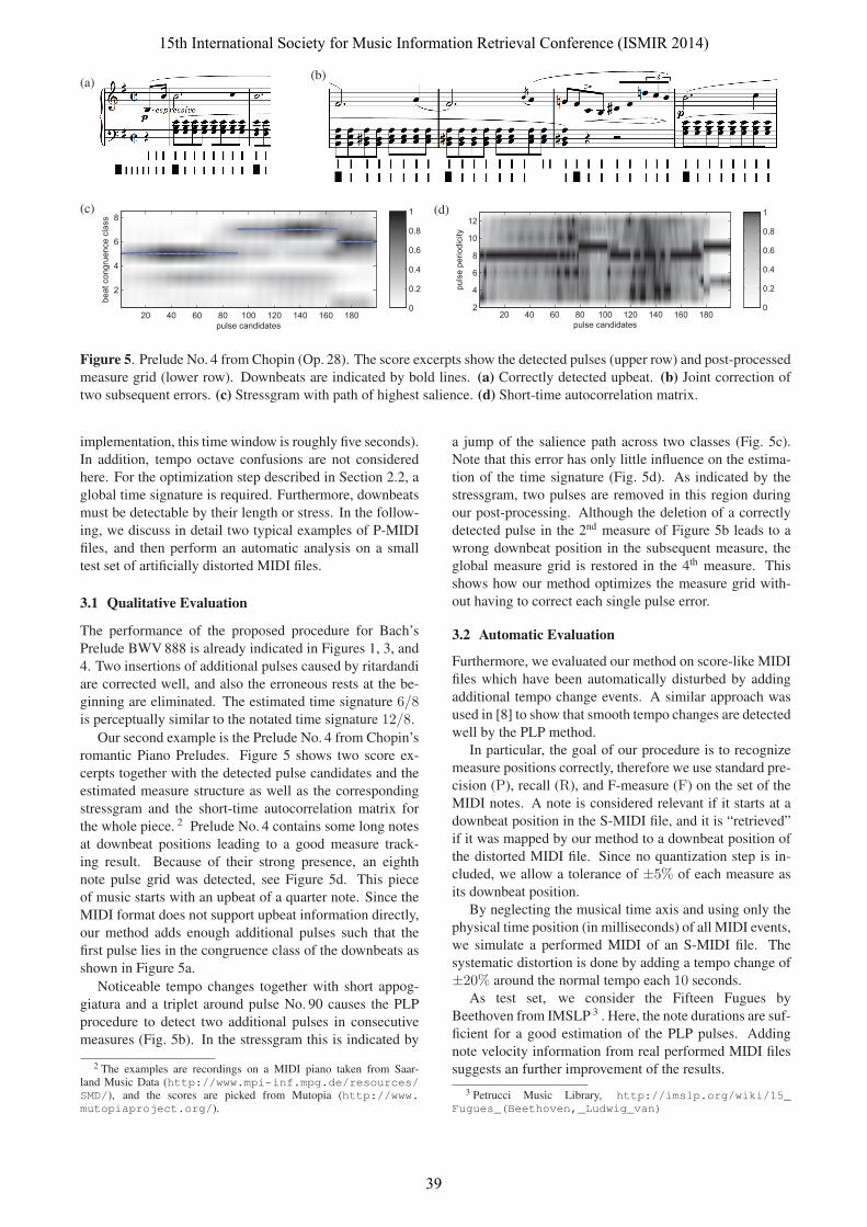
Figure 5. Prelude No. 4 from Chopin (Op. 28). The score excerpts show the detected pulses (upper row) and post-processed

measure grid (lower row). Downbeats are indicated by bold lines. (a) Correctly detected upbeat. (b) Joint correction of

two subsequent errors. (c) Stressgram with path of highest salience. (d) Short-time autocorrelation matrix.

implementation, this time window is roughly five seconds).

In addition, tempo octave confusions are not considered

here. For the optimization step described in Section 2.2, a

global time signature is required. Furthermore, downbeats

must be detectable by their length or stress. In the follow-

ing, we discuss in detail two typical examples of P-MIDI

files, and then perform an automatic analysis on a small

test set of artificially distorted MIDI files.

3.1 Qualitative Evaluation

The performance of the proposed procedure for Bach’s

Prelude BWV 888 is already indicated in Figures 1, 3, and

4. Two insertions of additional pulses caused by ritardandi

are corrected well, and also the erroneous rests at the be-

ginning are eliminated. The estimated time signature 6/8is perceptually similar to the notated time signature 12/8.

Our second example is the Prelude No. 4 from Chopin’s

romantic Piano Preludes. Figure 5 shows two score ex-

cerpts together with the detected pulse candidates and the

estimated measure structure as well as the corresponding

stressgram and the short-time autocorrelation matrix for

the whole piece. 2 Prelude No. 4 contains some long notes

at downbeat positions leading to a good measure track-

ing result. Because of their strong presence, an eighth

note pulse grid was detected, see Figure 5d. This piece

of music starts with an upbeat of a quarter note. Since the

MIDI format does not support upbeat information directly,

our method adds enough additional pulses such that the

first pulse lies in the congruence class of the downbeats as

shown in Figure 5a.

Noticeable tempo changes together with short appog-

giatura and a triplet around pulse No. 90 causes the PLP

procedure to detect two additional pulses in consecutive

measures (Fig. 5b). In the stressgram this is indicated by

2 The examples are recordings on a MIDI piano taken from Saar-land Music Data (http://www.mpi-inf.mpg.de/resources/SMD/), and the scores are picked from Mutopia (http://www.mutopiaproject.org/).

a jump of the salience path across two classes (Fig. 5c).

Note that this error has only little influence on the estima-

tion of the time signature (Fig. 5d). As indicated by the

stressgram, two pulses are removed in this region during

our post-processing. Although the deletion of a correctly

detected pulse in the 2nd measure of Figure 5b leads to a

wrong downbeat position in the subsequent measure, the

global measure grid is restored in the 4th measure. This

shows how our method optimizes the measure grid with-

out having to correct each single pulse error.

3.2 Automatic Evaluation

Furthermore, we evaluated our method on score-like MIDI

files which have been automatically disturbed by adding

additional tempo change events. A similar approach was

used in [8] to show that smooth tempo changes are detected

well by the PLP method.

In particular, the goal of our procedure is to recognize

measure positions correctly, therefore we use standard pre-

cision (P), recall (R), and F-measure (F) on the set of the

MIDI notes. A note is considered relevant if it starts at a

downbeat position in the S-MIDI file, and it is “retrieved”

if it was mapped by our method to a downbeat position of

the distorted MIDI file. Since no quantization step is in-

cluded, we allow a tolerance of ±5% of each measure as

its downbeat position.

By neglecting the musical time axis and using only the

physical time position (in milliseconds) of all MIDI events,

we simulate a performed MIDI of an S-MIDI file. The

systematic distortion is done by adding a tempo change of

±20% around the normal tempo each 10 seconds.

As test set, we consider the Fifteen Fugues by

Beethoven from IMSLP 3 . Here, the note durations are suf-

ficient for a good estimation of the PLP pulses. Adding

note velocity information from real performed MIDI files

suggests an further improvement of the results.

3 Petrucci Music Library, http://imslp.org/wiki/15_Fugues_(Beethoven,_Ludwig_van)


39

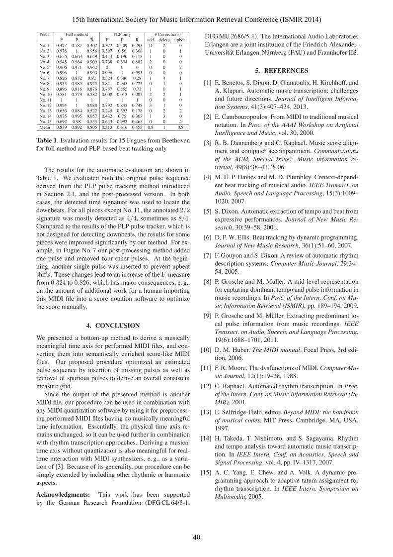
Piece Full method PLP only # CorrectionsF P R F P R add delete upbeat

No. 1 0.477 0.587 0.402 0.372 0.509 0.293 0 2 0No. 2 0.978 1 0.956 0.397 0.56 0.308 1 0 1No. 3 0.656 0.663 0.649 0.144 0.196 0.113 1 0 0No. 4 0.945 0.984 0.909 0.738 0.804 0.682 2 0 0No. 5 0.966 0.971 0.962 0 0 0 0 0 2No. 6 0.996 1 0.993 0.996 1 0.993 0 0 0No. 7 0.826 0.832 0.82 0.324 0.386 0.28 1 4 1No. 8 0.953 0.985 0.923 0.821 0.945 0.725 0 1 0No. 9 0.896 0.916 0.876 0.787 0.855 0.73 1 0 1No. 10 0.581 0.579 0.582 0.008 0.013 0.005 2 2 1No. 11 1 1 1 1 1 1 0 0 0No. 12 0.994 1 0.988 0.792 0.842 0.748 3 1 0No. 13 0.656 0.884 0.522 0.245 0.393 0.178 0 2 2No. 14 0.975 0.995 0.957 0.432 0.75 0.303 1 3 0No. 15 0.692 0.98 0.535 0.633 0.992 0.465 0 0 4

Mean 0.839 0.892 0.805 0.513 0.616 0.455 0.8 1 0.8

Table 1. Evaluation results for 15 Fugues from Beethoven

for full method and PLP-based beat tracking only

The results for the automatic evaluation are shown in

Table 1. We evaluated both the original pulse sequence

derived from the PLP pulse tracking method introduced

in Section 2.1, and the post-processed version. In both

cases, the detected time signature was used to locate the

downbeats. For all pieces except No. 11, the annotated 2/2signature was mostly detected as 4/4, sometimes as 8/4.

Compared to the results of the PLP pulse tracker, which is

not designed for detecting downbeats, the results for some

pieces were improved significantly by our method. For ex-

ample, in Fugue No. 7 our post-processing method added

one pulse and removed four other pulses. At the begin-

ning, another single pulse was inserted to prevent upbeat

shifts. These changes lead to an increase of the F-measure

from 0.324 to 0.826, which has major consequences, e. g.,

on the amount of additional work for a human importing

this MIDI file into a score notation software to optimize

the score manually.

4. CONCLUSION

We presented a bottom-up method to derive a musically

meaningful time axis for performed MIDI files, and con-

verting them into semantically enriched score-like MIDI

files. Our proposed procedure optimized an estimated

pulse sequence by insertion of missing pulses as well as

removal of spurious pulses to derive an overall consistent

measure grid.

Since the output of the presented method is another

MIDI file, our procedure can be used in combination with

any MIDI quantization software by using it for preprocess-

ing performed MIDI files having no musically meaningful

time information. Essentially, the physical time axis re-

mains unchanged, so it can be used further in combination

with rhythm transcription approaches. Deriving a musical

time axis without quantization is also meaningful for real-

time interaction with MIDI synthesizers, e. g., as a varia-

tion of [3]. Because of its generality, our procedure can be

simply extended by including other rhythmic or harmonic

aspects.

Acknowledgments: This work has been supported

by the German Research Foundation (DFG CL 64/8-1,

DFG MU 2686/5-1). The International Audio Laboratories

Erlangen are a joint institution of the Friedrich-Alexander-

Universitat Erlangen-Nurnberg (FAU) and Fraunhofer IIS.

5. REFERENCES

[1] E. Benetos, S. Dixon, D. Giannoulis, H. Kirchhoff, and

A. Klapuri. Automatic music transcription: challenges

and future directions. Journal of Intelligent Informa-tion Systems, 41(3):407–434, 2013.

[2] E. Cambouropoulos. From MIDI to traditional musical

notation. In Proc. of the AAAI Workshop on ArtificialIntelligence and Music, vol. 30, 2000.

[3] R. B. Dannenberg and C. Raphael. Music score align-

ment and computer accompaniment. Communicationsof the ACM, Special Issue: Music information re-trieval, 49(8):38–43, 2006.

[4] M. E. P. Davies and M. D. Plumbley. Context-depend-

ent beat tracking of musical audio. IEEE Transact. onAudio, Speech and Language Processing, 15(3):1009–

1020, 2007.

[5] S. Dixon. Automatic extraction of tempo and beat from

expressive performances. Journal of New Music Re-search, 30:39–58, 2001.

[6] D. P. W. Ellis. Beat tracking by dynamic programming.

Journal of New Music Research, 36(1):51–60, 2007.

[7] F. Gouyon and S. Dixon. A review of automatic rhythm

description systems. Computer Music Journal, 29:34–

54, 2005.

[8] P. Grosche and M. Muller. A mid-level representation

for capturing dominant tempo and pulse information in

music recordings. In Proc. of the Intern. Conf. on Mu-sic Information Retrieval (ISMIR), pp. 189–194, 2009.

[9] P. Grosche and M. Muller. Extracting predominant lo-

cal pulse information from music recordings. IEEETransact. on Audio, Speech, and Language Processing,

19(6):1688–1701, 2011.

[10] D. M. Huber. The MIDI manual. Focal Press, 3rd edi-

tion, 2006.

[11] F. R. Moore. The dysfunctions of MIDI. Computer Mu-sic Journal, 12(1):19–28, 1988.

[12] C. Raphael. Automated rhythm transcription. In Proc.of the Intern. Conf. on Music Information Retrieval (IS-MIR), 2001.

[13] E. Selfridge-Field, editor. Beyond MIDI: the handbookof musical codes. MIT Press, Cambridge, MA, USA,

1997.

[14] H. Takeda, T. Nishimoto, and S. Sagayama. Rhythm

and tempo analysis toward automatic music transcrip-

tion. In IEEE Intern. Conf. on Acoustics, Speech andSignal Processing, vol. 4, pp. IV–1317, 2007.

[15] A. C. Yang, E. Chew, and A. Volk. A dynamic pro-

gramming approach to adaptive tatum assignment for

rhythm transcription. In IEEE Intern. Symposium onMultimedia, 2005.


40

estimating musical time information from performed … · estimating musical time information from...

Documents