Statistics and Probability Letters 83 (2013) 812–819

Contents lists available at SciVerse ScienceDirect

Statistics and Probability Letters

journal homepage: www.elsevier.com/locate/stapro

Estimating genotyping error rates from parent–offspringdyadsØystein A. Haaland a, Hans J. Skaug a,b,∗

a Department of Mathematics, University of Bergen, Johannes Brunsgate 12, 5008 Bergen, Norwayb Institute of Marine Research. P.O. Box 1870, Nordnes. N-5817 Bergen, Norway

a r t i c l e i n f o

Article history:Received 11 April 2011Received in revised form 2 November 2012Accepted 11 November 2012Available online 3 December 2012

Keywords:DNA registerParent–offspring dyadGenotyping errorPedigreeBias

a b s t r a c t

A common approach when estimating the error rate of a DNA register is to genotype someof the individuals twice. Thismay be both expensive and time consuming. As an alternative,we present a new method for estimating genotyping errors based on parent–offspringdyads. The basic idea is that parent and offspring must share at least one allele per locus.Others have previously devised similar techniques, but depended on the assumption thatat most one error may occur per dyad. In this paper we examine the bias caused by thissimplification. Further, we apply our method on a data set from the Norwegian minkewhale DNA register, and find that the error rates are in the range of 0–0.0418, which iscomparable to those in the published literature.

© 2012 Elsevier B.V. All rights reserved.

1. Introduction

DNA registers are most widely known for their use in forensics, but such data bases are also playing an increasinglyimportant role in other fields, such as ecology (Blouin, 2003) and medicine (Ewen et al., 2000). Typing errors, i.e., theoccurrence of errors in the genetic analysis causing the inferred and true genotypes to differ, may severely affect theconclusions drawn from DNA profile data if not accounted for Pompanon et al. (2005). Most studies aiming at estimatingsuch rates involve scoring the same individual more than once (Paetkau, 2003; Bonin et al., 2004; Hoffman and Amos, 2005;Tintle et al., 2007; Haaland et al., 2011). However, this powerful and direct approach is not always available, e.g., due tofinancial reasons, or if the organism is small (Steinauer et al., 2008). In wildlife populations, mother–offspring dyads areoften easy to identify (Hoffman and Amos, 2005), and in medical research it is common to collect DNA profiles on pedigrees(Ewen et al., 2000; Sobel et al., 2002). Error rate estimation from such data, and parent–offspring data in particular, is thetheme of this paper.

At a locus an individual has two gene copies, one inherited from each parent, that are selected from a set of n possiblealleles (a1, . . . , an), so a parent and an offspring must necessarily share at least one allele per locus. This motivated thedevelopment of statistical techniques enabling us to estimate genotyping error rates from parent–offspring dyads of DNAprofiles. Similar methods have been presented by others (Douglas et al., 2002; Saunders et al., 2007), but rest on theassumption that no more than one error occurs in each family under consideration (in our case this translates to one errorper parent–offspring dyad). We also consider microsatellites (more than two alleles per locus) instead of SNPs (two allelesper locus) (Douglas et al., 2002).

∗ Corresponding author at: Department of Mathematics, University of Bergen, Johannes Brunsgate 12, 5008 Bergen, Norway.E-mail address: hans.skaug@math.uib.no (H.J. Skaug).

0167-7152/$ – see front matter© 2012 Elsevier B.V. All rights reserved.doi:10.1016/j.spl.2012.11.009

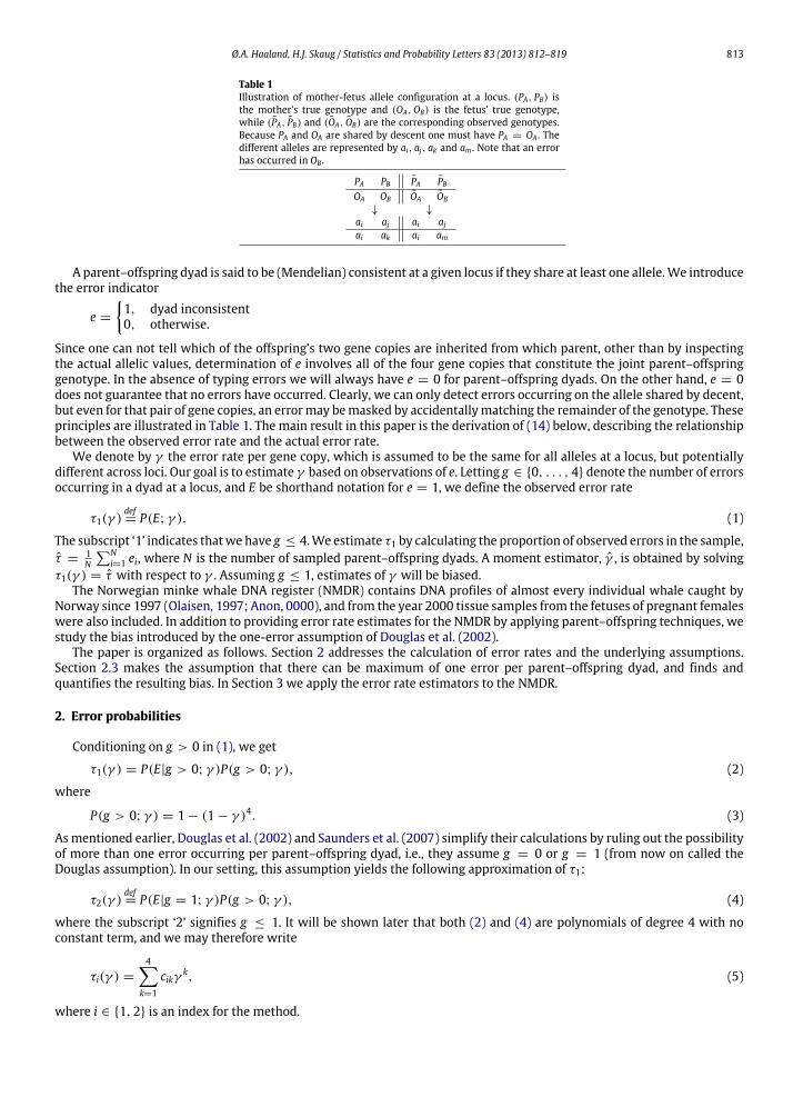
Ø.A. Haaland, H.J. Skaug / Statistics and Probability Letters 83 (2013) 812–819 813

Table 1Illustration of mother-fetus allele configuration at a locus. (PA, PB) isthe mother’s true genotype and (OA,OB) is the fetus’ true genotype,while (PA, PB) and (OA, OB) are the corresponding observed genotypes.Because PA and OA are shared by descent one must have PA = OA . Thedifferent alleles are represented by ai, aj, ak and am . Note that an errorhas occurred in OB .

PA PB PA PBOA OB OA OB

↓ ↓

ai aj ai ajai ak ai am

A parent–offspring dyad is said to be (Mendelian) consistent at a given locus if they share at least one allele.We introducethe error indicator

e =

1, dyad inconsistent0, otherwise.

Since one can not tell which of the offspring’s two gene copies are inherited from which parent, other than by inspectingthe actual allelic values, determination of e involves all of the four gene copies that constitute the joint parent–offspringgenotype. In the absence of typing errors we will always have e = 0 for parent–offspring dyads. On the other hand, e = 0does not guarantee that no errors have occurred. Clearly, we can only detect errors occurring on the allele shared by decent,but even for that pair of gene copies, an errormay bemasked by accidentallymatching the remainder of the genotype. Theseprinciples are illustrated in Table 1. The main result in this paper is the derivation of (14) below, describing the relationshipbetween the observed error rate and the actual error rate.

We denote by γ the error rate per gene copy, which is assumed to be the same for all alleles at a locus, but potentiallydifferent across loci. Our goal is to estimate γ based on observations of e. Letting g ∈ {0, . . . , 4} denote the number of errorsoccurring in a dyad at a locus, and E be shorthand notation for e = 1, we define the observed error rate

τ1(γ )def= P(E; γ ). (1)

The subscript ‘1’ indicates thatwe have g ≤ 4.We estimate τ1 by calculating the proportion of observed errors in the sample,τ =

1N

Ni=1 ei, where N is the number of sampled parent–offspring dyads. A moment estimator, γ , is obtained by solving

τ1(γ ) = τ with respect to γ . Assuming g ≤ 1, estimates of γ will be biased.The Norwegian minke whale DNA register (NMDR) contains DNA profiles of almost every individual whale caught by

Norway since 1997 (Olaisen, 1997; Anon, 0000), and from the year 2000 tissue samples from the fetuses of pregnant femaleswere also included. In addition to providing error rate estimates for the NMDR by applying parent–offspring techniques, westudy the bias introduced by the one-error assumption of Douglas et al. (2002).

The paper is organized as follows. Section 2 addresses the calculation of error rates and the underlying assumptions.Section 2.3 makes the assumption that there can be maximum of one error per parent–offspring dyad, and finds andquantifies the resulting bias. In Section 3 we apply the error rate estimators to the NMDR.

2. Error probabilities

Conditioning on g > 0 in (1), we get

τ1(γ ) = P(E|g > 0; γ )P(g > 0; γ ), (2)

where

P(g > 0; γ ) = 1 − (1 − γ )4. (3)

As mentioned earlier, Douglas et al. (2002) and Saunders et al. (2007) simplify their calculations by ruling out the possibilityof more than one error occurring per parent–offspring dyad, i.e., they assume g = 0 or g = 1 (from now on called theDouglas assumption). In our setting, this assumption yields the following approximation of τ1:

τ2(γ )def= P(E|g = 1; γ )P(g > 0; γ ), (4)

where the subscript ‘2’ signifies g ≤ 1. It will be shown later that both (2) and (4) are polynomials of degree 4 with noconstant term, and we may therefore write

τi(γ ) =

4k=1

cikγ k, (5)

where i ∈ {1, 2} is an index for the method.

814 Ø.A. Haaland, H.J. Skaug / Statistics and Probability Letters 83 (2013) 812–819

2.1. Assumptions

At a given locus, let (PA, PB) be the parent’s genotype, and similarly let (OA,OB) be the offspring’s genotype (see Table 1).Without loss of generality, we take PA and OA to be the allele passed on by the parent to the offspring, so that PA = OA.While these are the true genotypes, we denote by (PA, PB) and (OA, OB) the observed genotypes, i.e., the result of the geneticanalysis. In the absence of typing errors we must have PA = PA, . . . ,OB = OB. An error is defined as the replacement of thetrue genotype with a genotype selected at random assuming a uniform distribution (see Assumption 3 below). As we willcome back to in Section 2.2, both τ1 and τ2 depend on γ , as well as other quantities.

In order to derive the mathematical expression for (1), we shall need the following definitions:

• P1A denotes the event that an error occurs in PA. Essentially, thismeans that PA = PA, butwe include the possibility that the

substituted allele is the same as the original, as is done in Hoffman and Amos (2005) (see Assumption 3 below). Similarly,P1B ,O

1A and O1

B are the events that errors occur in PB,OA and OB, respectively.• P0

A means that no error occurs in PA. The same applies for PB,OA and OB.• At the locus, a1, . . . , an is the set of alleles.• Population allele frequencies: fi = P(ai), i = 1, . . . , n.

The following will be assumed:

1. The population is in Hardy–Weinberg equilibrium: P(PA = ai, PB = aj) = fifj.2. Errors are independently distributed across gene copies.3. Uniform substitution rates:

PPA = ai|P1

A

=

1n, i = 1, . . . , n. (6)

The appropriateness of Assumption 3 will be considered further in Section 4.

2.2. An expression for τ1

Nowwe arewell equipped to start our quest for τ1(γ ), and begin by noticing that due to Assumption 2 above, and becauseerrors on OB and PB are always unobserved,

τ1(γ ) = PE, P1

A ,O1A

+ P

E, P0

A ,O1A

+ P

E, P1

A ,O0A

= γ 2P

E|P1

A ,O1A

+ 2γ (1 − γ )P

E|P1

A ,O0A

. (7)

Then we consider the first part of the right hand side of (7).

PE|P1

A ,O1A

= P

OA = PA, OA = PB, OB = PA, OB = PB|P1

A ,O1A

= 1 − P

OA = PA ∪ OA = PB ∪ OB = PA ∪ OB = PB|P1

A ,O1A

. (8)

Introducing the short hand notation

W1 : OA = PA|P1A ,O

1A

, X1 : OA = PB|

P1A ,O

1A

,

Y1 : OB = PA|P1A ,O

1A

, Z1 : OB = PB|

P1A ,O

1A

,

and substituting into (8) yields

PE|P1

A ,O1A

= 1 − P(W1) − P(X1) − P(Y1) − P(Z1)

+ P(W1, X1) + P(W1, Y1) + P(W1, Z1) + P(X1, Y1) + P(X1, Z1) + P(Y1, Z1)− P(W1, X1, Y1) − P(W1, X1, Z1) − P(W1, Y1, Z1) − P(X1, Y1, Z1) + P(W1, X1, Y1, Z1). (9)

In order to better be able to handle PB and OB, we define

Gidef= P

PB = ai

. (10)

Assumption 2 yields Gi = POB = ai

, and according to Assumptions 1 and 3, (10) becomes

Gi = P(P0B )fi + P(P1

B )1n

= (1 − γ )fi + γ1n. (11)

Ø.A. Haaland, H.J. Skaug / Statistics and Probability Letters 83 (2013) 812–819 815

Now we may utilize (11) to calculate each of the terms in (9),

P(W1) = P(X1) = P(Y1) =1n, P(Z1) =

ni=1

G2i ,

P(W1, X1) = P(W1, Y1) = P(X1, Y1) =1n2

,

P(W1, Z1) = P(X1, Z1) = P(Y1, Z1) =1n

ni=1

G2i ,

P(W1, X1, Y1) = P(W1, X1, Z1) = P(W1, Y1, Z1) = P(X1, Y1, Z1) =1n2

ni=1

G2i ,

P(W1, X1, Y1, Z1) =1n2

ni=1

G2i ,

and hence

PE|P1

A ,O1A

=

1 −

3n

+3n2

1 −

ni=1

G2i

. (12)

Using the same approach for PE|P1

A ,O0A

, where

W2 : OA = PA|P1A ,O

0A

, X2 : OA = PB|

P1A ,O

0A

,

Y2 : OB = PA|P1A ,O

0A

, Z2 : OB = PB|

P1A ,O

0A

,

we get

P(W2) = P(Y2) =1n, P(X2) =

ni=1

fiGi, P(Z2) =

ni=1

G2i ,

P(W2, X2) = P(W2, Y2) = P(X2, Y2) =1n

ni=1

fiGi,

P(W2, Z2) = P(Y2, Z2) =1n

ni=1

G2i , P(X2, Z2) =

ni=1

fiG2i ,

P(W2, X2, Y2) = P(W2, X2, Z2) = P(W2, Y2, Z2) = P(X2, Y2, Z2) =1n

ni=1

fiG2i ,

P(W2, X2, Y2, Z2) =1n

ni=1

fiG2i ,

so that

PE|P1

A ,O0A

= 1 −

2n

−

1 −

2n

ni=1

G2i −

1 −

3n

ni=1

fiGi +

1 −

3n

ni=1

fiG2i . (13)

Substituting (12) and (13) in (7), gives

τ1(γ ) = 2γ (1 − γ )

1 −

2n

−

1 −

2n

ni=1

G2i −

1 −

3n

ni=1

fiGi +

1 −

3n

ni=1

fiG2i

+ γ 21 −

3n

+3n2

1 −

ni=1

G2i

, (14)

and our goal is achieved. If fi =1n , (11) reduces to Gi =

1n , but generally G2

i is a quadratic polynomial in γ . Because both(12) and (13) are polynomials in Gi of degree 2, we see from (14) that τ1 is a polynomial in γ of degree 4 with no constantterm. Assuming the allele frequencies, fi, are known, the coefficients c1k from (5) can easily be obtained using software (e.g.,Maple 14).

816 Ø.A. Haaland, H.J. Skaug / Statistics and Probability Letters 83 (2013) 812–819

2.3. The Douglas assumption

Finding a mathematical expression for (4) is more straightforward than for (2). Let H be the heterozygosity, a measureof genetic diversity at a locus

H = 1 −

i f

2i

, of the locus under consideration. When PB = OB, P(E|g = 1) is always zero,

so that for i = j = k

P(E|g = 1) = 2i=j

P(E, PA = OA = PB = ai,OB = aj|g = 1)

+

i=j=k

P(E, PA = OA = ai, PB = aj,OB = ak|g = 1)

=n − 12n

i=j

f 2i fj +n − 22n

i=j=k

fifjfk

= H −12

+12

ni=1

f 3i −

5H − 31 −

ni=1

f 3i

2n

, (15)

becausen

i=j f2i fj = (1 − H) −

ni=1 f

3i and

ni=j=k fifjfk = 1 − 3(1 − H) + 2

ni=1 f

3i . We see that (15) is free of γ , so we

get from (4) that τ2 is also a polynomial of degree 4 with no constant term.If needed, (14) too could be expressed in terms of H and

ni=1 f

3i , but writing it out would require more space than the

current equation.

2.4. Comparison

Remember that estimates for γ can be obtained by solving (5) for a given value of the observed error rate, τ . Denote byγi the solution of (5) for τi. Calculating the cik of (5) yields c11 = c21 ≡ c1, but c1k = c2k for k > 1. The bias of γ2 relative toγ1 is expressed by

B(τ ) =γ2(τ )

γ1(τ )− 1. (16)

Since τi = 0 ⇒ γi = 0, we have γ2(0)/γ1(0) = 0/0. Still, B(0) = 0 by l’Hôpital’s rule, because ddτ γ1(0) =

ddτ γ2(0) = 1/c1.

The first order Taylor expansion of (16) around τ = 0 yields

B(τ ) = Sτ + O(τ 2), (17)

where S = (c12 − c22)/c21 . Multiple genotyping errors in a single parent–offspring dyad are more likely when the errorrate is high, so we expect the absolute value of B(τ ) to increase with τ . Denoting by τact the actual error rate per dyad, weessentially have

τ = τactP(E|g > 0) ⇒ τact = τ/P(E|g > 0). (18)

Because P(E|g > 0) > P(E|g = 1), exchanging the former for the latter in (18), we expect inflated estimates of τ , andtherefore also of γ . It follows that B(τ ) should be positive. We therefore postulate that S > 0 in general, but have no proofof this.

We wish to examine the asymptotic behavior of S when n → ∞. Generally, our focus is on a systemwhere one allele, a1say, is dominating, and the others are equally rare. We assume

fi =1 − f1n − 1

, i = 2, . . . , n,

where f1 ∈ (0, 1) is fixed. Hence, we get

H = 1 − f 21 −(1 − f1)2

n − 1→ 1 − f 21 , (19)

andn

i=1

f 3i = f 31 +(1 − f1)3

(n − 1)2→ f 31 , (20)

as n → ∞. If instead f1 = f2 = · · · = fn = 1/n, (19) translates to limn→∞ H = 1, and (20) to limn→∞

ni=1 f

3i = 0. Because

S can be expressed in terms of n and f1 by utilizing (19) and (20), numerical experiments yield S > 0 when n ≥ 3 and

Ø.A. Haaland, H.J. Skaug / Statistics and Probability Letters 83 (2013) 812–819 817

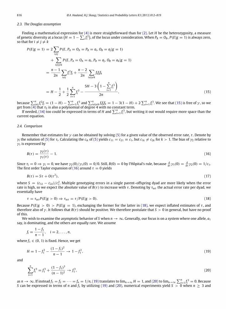
Table 2Values of B(0.05) from (16) and S ∗ 0.05 from (17),varying n and f1 . Because f1 by definition is the mostfrequent allele, not all values of f1 are possible for all n.

f1 n H B(0.05) S ∗ 0.05

0∞ 1 0.027 0.02510 – – –4 – – –

√0.05

∞ 0.95 0.034 0.03210 0.88 0.046 0.0414 – – –

√0.10

∞ 0.90 0.043 0.04010 0.85 0.055 0.0494 0.75 0.098 0.078

√0.25

∞ 0.75 0.082 0.07610 0.72 0.097 0.0864 0.67 0.142 0.112

√0.33

∞ 0.67 0.118 0.11010 0.65 0.137 0.1224 0.61 0.190 0.148

√0.50

∞ 0.50 0.261 0.24410 0.49 0.295 0.2614 0.47 0.387 0.293

f1 ∈ [0, 1]. Consequentially, the bias is low for low genotyping error rates, which only moderately affect statistical analysis,but high for high error rates, for which the impact is more serious. Taking the limit n → ∞, we get

S∞(f1) = limn→∞

S(f1, n) =2 + 3f 21 − 3f 31

4(f 21 − f1 − 1)2(f1 − 1)2. (21)

Varying f1, we see that limf1→1 S∞(f1) = ∞. This has the interpretation that PA = PB = OA = OB = a1 (Table 1), so thatall dyads are Mendelian consistent unless at least two errors occur. However, because we let n → ∞, Assumption 3 aboutuniform substitution rates (6) assures that all potentiallyMendelian inconsistent dyads (i.e., dyadswhere (P1

A , P1B )∪(O1

A,O1B)

is true) will always be detected. Considering the other extreme, we get

limf1→0

S∞(f1) =12. (22)

Hence, the Douglas assumption will always cause some bias. Letting the allele frequencies be uniformly distributed (f1 =

1/n), (22) can be written

limn→∞

S1n, n

=12.

This leads to all errors at the shared gene copies being detected, or P(E|P1A ∪ O1

A) = 1 (Table 1). If f1 is fixed, letting n → ∞

ensures that among the alleles, only a1 mayappearmore thanoncewithin a dyad. Thus, the dyad is not necessarilyMendelianinconsistent, even if an error was committed at a shared gene copy. E.g., if PA = PB = a1 (Table 1), a single error at PA wouldnot be detected.

Direct numerical evaluation of (16) for different values of n(n ∈ {4, 10, ∞}) and f1f1 ∈

0,

√0.05,

√0.10,

√0.25,

√0.33,

√0.50

supports the above findings (Table 2). We considered values of τ that are greater than 0.05 to be of limited

interest (Pompanon et al., 2005), and therefore constructed Table 2 using τ = 0.05. As a consequence of Assumption 3 aboutuniform substitution rates (6), for a given f1, errors at the shared gene copies have a higher likelihood of being discoveredwhen n is large (Table 2). When f1 is high, the heterozygosity H is low, and detecting errors becomes more difficult. Forexample, in scenarios where PB = OB (Table 1), the dyad will always be Mendelian consistent unless at least two errorsoccur, and if PA = PB (Table 1), a single error can only be detected if it occurs at OA. The less likely one is to discovera single error, the more likely it is that a Mendelian inconsistent dyad has at least two errors. Thus, the bias due to theDouglas assumption is greater. This is confirmed in Table 2, where B(0.05) decreases with decreasing f1, and increases withdecreasing n. The top row in Table 2 gives a lower limit of B(0.05).

3. A case study: the Norwegian minke whale DNA register (NMDR)

Error rate estimation from parent–offspring data is the theme of this paper. We have used the NMDR in order to applyour techniques on real data. Haaland et al. (2011) provides a more elaborate description of the NMDR.

818 Ø.A. Haaland, H.J. Skaug / Statistics and Probability Letters 83 (2013) 812–819

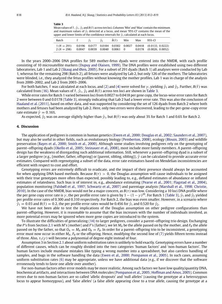
Table 3Meanvalues of τ , γ1, γ2 andB(τ ) across ten loci. Columns ‘Min’ and ‘Max’ contain theminimumand maximum values of γ1 detected at a locus, and mean ‘95%-CI’ contains the mean of theupper and lower limits of the confidence intervals for γ1 calculated at each locus.

Batch τ γ1 γ2 B(τ ) Min Max 95%-CI

1 (N = 291) 0.0196 0.0177 0.0184 0.0302 0.0027 0.0418 (0.0133, 0.0222)2 (N = 298) 0.0047 0.0039 0.0040 0.0061 0 0.0178 (0.0026, 0.0052)

In the years 2000–2006 DNA profiles for 589 mother-fetus dyads were entered into the NMDR, with each profileconsisting of 10 microsatellite markers (Dupuy and Olaisen, 1999). The DNA profiles were established using two differentlaboratories, Lab 1 and Lab 2 (Skaug and Øien, 2005). For a subset of 291 dyads (Batch 1) all analyses were conducted by Lab1, whereas for the remaining 298 (Batch 2), all fetuses were analyzed by Lab 2, but only 126 of the mothers. The laboratorieswere blinded, i.e., they analyzed the fetus profiles without knowing the mother profiles. Lab 1 was in charge of the analysisfrom 2000–2002, and Lab 2 from 2003–2006.

For both batches, τ was calculated at each locus, and (2) and (4) were solved for γ , yielding γ1 and γ2. Further, B(τ ) wascalculated from (16). Mean values of τ , γ1, γ2 and B(τ ) across ten loci are shown in Table 3.

While error rates for Batch 1 varied between loci from0.0027 to 0.0418 per gene copy, the locus-wise error rates for Batch2 were between 0 and 0.0178 (Table 3), strongly indicating that Lab 2 had a lower error rate. This was also the conclusion ofHaaland et al. (2011), based on other data, and was supported by considering the set of 126 dyads from Batch 2 where bothmothers and fetuses had been analyzed by Lab 2. Here, only two errors were discovered, leading to the per-gene-copy errorrate estimate γ = 0.16%.

As expected, γ2 was on average slightly higher than γ1, but B(τ ) was only about 3% for Batch 1 and 0.6% for Batch 2.

4. Discussion

The application of pedigrees is common in human genetics (Ewen et al., 2000; Douglas et al., 2002; Saunders et al., 2007),but may also be useful in other fields, such as evolutionary biology (Pemberton, 2008), ecology (Blouin, 2003) and wildlifepreservation (Bayes et al., 2000; Smith et al., 2000). Although some studies involving pedigrees rely on the genotyping ofparent–offspring dyads (Okello et al., 2005; Steinauer et al., 2008), most include more family members. A parent–offspringdesign has the weakness of disregarding such additional information. Still, whenever a parent–offspring dyad is a subset ofa larger pedigree (e.g., {mother, father, offspring} or {parent, sibling, sibling}), γ can be calculated to provide accurate errorestimates. Compared with regenotyping a subset of the data, error rate estimators based on Mendelian inconsistencies areefficient with respect to cost and effort.

Genotyping errors are extremely difficult to eradicate, and the impact of their presence should always be accountedfor when applying DNA based methods. Because B(τ ) > 0, the Douglas assumption will cause individuals to be assignedwith their true genotypes more often than expected, possibly leading to, e.g., deflated estimates of abundance or inflatedestimates of relatedness. Such bias is of interest in, e.g., abundance estimating (Pearse et al., 2001; Flagstad et al., 2004),population monitoring (Palsbøll et al., 1997; Schwartz et al., 2007) and parentage analysis (Marshall et al., 1998; Christie,2010). In the case of the NMDR, bias would not be amajor concern, as B(τ )was low. Considering a 10 loci DNA profile wherethe per gene copy error rate is γ , the per profile error rate is given by 1− (1− γ )20. For Batch 1 (Table 3), γ1 and γ2 yieldedper profile error rates of 0.300 and 0.310 respectively. For Batch 2, the bias was even smaller. However, in a scenario whereγ1 = 0.03 and B(τ ) = 0.2, the per profile error rates would be 0.456 for γ1 and 0.520 for γ2.

We have not been able to test the implications of the Douglas assumption on other pedigree configurations thanparent–offspring. However, it is reasonable to assume that the bias increases with the number of individuals involved, asmore potential errors may be ignored when more gene copies are introduced to the system.

To illustrate the difficulties of generalizing (14) to larger pedigrees, consider a parent–offspring trio design. Exchangingthe P ’s from Section 2.1 withM ’s (mother) and F ’s (father), we letMA be the allele passed on by the mother, and FB the allelepassed on by the father, so that OA = MA and OB = FB. In order for a parent–offspring trio to be inconsistent, a genotypingerror must now occur in either MA, FB or the offspring. Hence, modifying the second line of (7) yields fifteen terms insteadof three. Also, τ1(γ ) will become a polynomial of degree eight instead of four.

Assumption 3 in Section 2.1 about uniform substitution rates is unlikely to hold exactly. Genotyping errors have a numberof different causes, which can be roughly divided into the two categories ‘human factors’ and ‘non-human factors’. Thehuman factors include mundane mistakes like typing a wrong number into a spreadsheet, but also careless handling ofsamples, and bugs in the software handling the data (Ewen et al., 2000; Pompanon et al., 2005). In such cases, assuminguniform substitution rates (6) may be appropriate, unless we have additional data (e.g., if we discover that the softwareerroneously tends to favor one allele over another).

For non-human factors other errormodelsmay bemore realistic. Among such factors we have low quality/quantity DNA,biochemical artifacts, and interactions betweenDNAmolecules (Pompanon et al., 2005; Hoffman andAmos, 2005). Commonerrors due to non-human factors are so called ‘allelic dropouts’ and ‘null alleles’ (causing the genotype at a heterozygouslocus to appear homozygous), and ‘false alleles’ (a false allele appearing close to a true allele, causing the genotype at a

Ø.A. Haaland, H.J. Skaug / Statistics and Probability Letters 83 (2013) 812–819 819

homozygous locus to appear heterozygous) (Pompanon et al., 2005). Both null alleles, allelic dropouts and false alleles havethat in common that they depend on the other alleles at the genotype. Because allelic dropouts and null alleles at PA or OAwill always be detected unless OB = PB, error rates derived assuming uniform substitution may be inflated. However, theimpact of false alleles is the opposite, as errors at homozygous genotypes cannot be detected unless both gene copies arefalsely recorded.

The fi from (14) and (15) have to be estimated from the data in order to obtain the coefficients cik from (5). Themore dataavailable, and the higher the allele frequency, the more accurate the estimate will be.

5. Tables and figures

See Tables 1–3.

References

Anon. Progress report from Norway to be presented to the scientific committee of the international whaling commission, May.Bayes, M.K., Smith, K.L., Alberts, S.C., Altmann, J., Bruford, M.W., 2000. Conservation Genetics 1, 173–176.Blouin, M.S., 2003. TRENDS in Ecology and Evolution 18.Bonin, A., Bellemain, E., Eidesen, P.B., Pompanon, F., Brochmann, C., Taberlet, P., 2004. Molecular Ecology 13, 3261–3273.Christie, M.R., 2010. Molecular Ecology Resources 10, 115–128.Douglas, J.A., Skol, A.D., Boehnke, M., 2002. American Journal of Human Genetics 70, 487–495.Dupuy, B., Olaisen, B., 1999. Typing Procedure for The Norwegian Minke Whale DNA Register.Ewen, K.R., Bahlo, M., Treloar, S.A., Levinson, D.F., Mowry, B., Barlow, J.W., Foote, S.J., 2000. American Journal of Human Genetics 67, 727–736.Flagstad, O., Hedmark, E., Landa, A., Brøseth, H., Persson, J., Andersen, R., Segerstrom, P., Ellegren, H., 2004. Conservation Biology 18, 676–688.Haaland, O.A., Glover, K.A., Seliussen, B.S., Skaug, H.J., 2011. BMC Genetics 12, 36.Hoffman, J.I., Amos, W., 2005. Molecular Ecology 14, 599–612.Marshall, T.C., Slate, J., Kruuk, L.E., Pemberton, J.M., 1998. Molecular Ecology 7, 639–655.Okello, J.B.A., Wittemyer, G., Rasmussen, H.B., Douglas-Hamilton, I., Nyakaana, S., Arctander, P., Siegismund, H.R., 2005. Journal of Hered 96, 679–687.Olaisen, B., 1997. Proposed specification for a Norwegian DNA database register for minke whales, Paper SC/49/NA1 presented to the Scientific Committee

of the International Whaling Commission.Paetkau, D., 2003. Molecular Ecology 12, 1375–1387.Palsbøll, P.J., Allen, J., Bérubé, M., Clapham, P.J., Feddersen, T.P., Hammond, P.S., Hudson, R.R., Jørgensen, H., Katona, S., Larsen, A.H., Larsen, F., Lien, J., Mattila,

D.K., Sigurjónsson, J., Sears, R., Smith, T., Sponer, R., Stevick, P., Oien, N., 1997. Nature 388, 767–769.Pearse, D.E., Eckerman, C.M., Janzen, F.J., Avise, J.C., 2001. Molecular Ecology 10, 2711–2718.Pemberton, J.M., 2008. Proceedings Biological Sciences 275, 613–621.Pompanon, F., Bonin, A., Bellemain, E., Taberlet, P., 2005. Nature Reviews Genetics 6, 847–859.Saunders, I.W., Brohede, J., Hannan, G.N., 2007. Genomics 90, 291–296.Schwartz, M.K., Luikart, G., Waples, R.S., 2007. Trends in Ecology & Evolution 22, 25–33.Skaug, H.J., Øien, N., 2005. Journal of Cetecean Research and Management 7 (2), 113–117.Smith, K.L., Alberts, S.C., Bayes, M.K., Bruford, M.W., Altmann, J., Ober, C., 2000. American Journal of Primatology 51, 219–227.Sobel, E., Papp, J.C., Lange, K., 2002. American Journal of Human Genetics 70, 496–508.Steinauer, M.L., Agola, L.E., Mwangi, I.N., Mkoji, G.M., Loker, E.S., 2008. Infections, Genetics and Evolution 8, 68–73.Tintle, N.L., Gordon, D., McMahon, F.J., Finch, S.J., 2007. Statistical Applications in Genetics and Molecular Biology 6, Article 4.