estimated abundance of adult fall chum salmon in the upper

Estimated Abundance of Adult Fall Chum Salmon in the Upper Yukon River, Alaska, 1997

Alaska Fisheries Technical Report Number 56

by

Tevis J. UnderwoodSteven P. Klosiewski 1

Judith A. Gordon2

Jeff L. MelegariRandolf J. Brown

Key words: fall chum salmon, Oncorhynchus keta, mark, recapture, Darroch, population estimate, selective sampling, Yukon River, fish wheel, tag

U.S. Fish and Wildlife Service, Fairbanks Fishery Resource Office101 12th Ave., Box 17, Room 222, Fairbanks, Alaska, 99701

1 U.S. Fish and Wildlife Service, Division of Fishery Resources,1011 East Tudor Road, Anchorage, Alaska, 99503

2 U.S Fish and Wildlife Service, Abernathy Salmon Culture Technical Center,1440 Abernathy Road, Longview, Washington 98632

February 2000

ii

Disclaimers

The mention of trade names or commercial products in this report does not constituteendorsement of recommendation for use by the Federal government.

The U.S. Department of the Interior prohibits discrimination in programs on the basis ofrace, color, national origin, religion, sex, age, or disability. If you believe that you have beendiscriminated against in any program, activity, or facility operated by the U.S. Fish and WildlifeService or if you desire further information please write to:

U.S. Department of the InteriorOffice for Equal Opportunity

1849 C. Street, NWWashington, D. C. 20240

The correct citation for this report is:

Underwood, T. J., S. P. Klosiewski, J. A. Gordon, J. L. Melegari, and R. J. Brown. 2000. Estimated abundance of adult fall Chum salmon in the upper Yukon River, Alaska, 1997. U. S.Fish and Wildlife Service, Fairbanks Fishery Resource Office, Alaska Fisheries TechnicalReport Number 56, Fairbanks, Alaska.

iii

Abstact

Weekly and a seasonal estimates of fall chum salmon were made between July 21 andSeptember 20, 1997 on the Yukon River above the Tanana River, Alaska. Two fish wheels wereused to capture and spaghetti tag 18,631 fall chum salmon. A second pair of fish wheels wereused from July 22 to September 28 to capture and examine 40,978 fall chum salmon for tagsnear the village of Rampart, Alaska, 50 km upstream. Excluding multiple recaptures, 1,872 fishwere recaptured. The calculated seasonal Darroch population estimate of 369,546 + 17,386(95% CI), was within 15% of an independent estimate of 430,493 fall chum salmon in the upperYukon River. Most tagged fish were caught within the week they were marked. Tag loss wasexamined at numerous locations within the drainage using primary and secondary marks and notag loss was documented. Fish that were captured for tagging from the north and south banksmixed randomly between the tagging and recapture sites. The probability of recapture, theproduct of the probabilities of capture and movement, were found to be associated with theinteraction length and sex during the third week of tagging and associated with the main effectsof length and sex in week eight. Bias was still considered small because differences in thestratified and unstratified estimate was negligible. No other potential selective sampling wasdetected via statistical analysis. We conclude that the Darroch estimator is a reasonable methodof calculating abundance of fall chum salmon in the upper Yukon River.

iv

Table of Contents

Abstact . . . . . . . . . . . . . . . . . . . . . . . . . . . . . . . . . . . . . . . . . . . . . . . . . . . . . . . . . . . . . . . . . . . . . iii

List of Tables . . . . . . . . . . . . . . . . . . . . . . . . . . . . . . . . . . . . . . . . . . . . . . . . . . . . . . . . . . . . . . . . vi

List of Figures . . . . . . . . . . . . . . . . . . . . . . . . . . . . . . . . . . . . . . . . . . . . . . . . . . . . . . . . . . . . . . viii

Introduction . . . . . . . . . . . . . . . . . . . . . . . . . . . . . . . . . . . . . . . . . . . . . . . . . . . . . . . . . . . . . . . . . . 1

Study Area . . . . . . . . . . . . . . . . . . . . . . . . . . . . . . . . . . . . . . . . . . . . . . . . . . . . . . . . . . . . . . . . . . . 2

Methods . . . . . . . . . . . . . . . . . . . . . . . . . . . . . . . . . . . . . . . . . . . . . . . . . . . . . . . . . . . . . . . . . . . . . 3Assumptions of the Estimator . . . . . . . . . . . . . . . . . . . . . . . . . . . . . . . . . . . . . . . . . . . . . . 3Marking Site Sampling Procedures . . . . . . . . . . . . . . . . . . . . . . . . . . . . . . . . . . . . . . . . . . 4Recapture Site Sampling Procedures . . . . . . . . . . . . . . . . . . . . . . . . . . . . . . . . . . . . . . . . . 5Analysis of Tagging and Recovery Wheel Data . . . . . . . . . . . . . . . . . . . . . . . . . . . . . . . . 6

Migration times . . . . . . . . . . . . . . . . . . . . . . . . . . . . . . . . . . . . . . . . . . . . . . . . . . . 6Tag retention . . . . . . . . . . . . . . . . . . . . . . . . . . . . . . . . . . . . . . . . . . . . . . . . . . . . . 6Assessment of condition and color classifications . . . . . . . . . . . . . . . . . . . . . . . . 6Equal probability of capture and movement to recapture strata . . . . . . . . . . . . . . 7Random mixing . . . . . . . . . . . . . . . . . . . . . . . . . . . . . . . . . . . . . . . . . . . . . . . . . . . 7Abundance estimate . . . . . . . . . . . . . . . . . . . . . . . . . . . . . . . . . . . . . . . . . . . . . . . . 8CPUE versus estimated abundance . . . . . . . . . . . . . . . . . . . . . . . . . . . . . . . . . . . . 9

Analysis of Recapture to Capture Ratios . . . . . . . . . . . . . . . . . . . . . . . . . . . . . . . . . . . . . . 9Incomplete reporting . . . . . . . . . . . . . . . . . . . . . . . . . . . . . . . . . . . . . . . . . . . . . . . 9Immigration of unmarked fish . . . . . . . . . . . . . . . . . . . . . . . . . . . . . . . . . . . . . . . . 9Tag loss . . . . . . . . . . . . . . . . . . . . . . . . . . . . . . . . . . . . . . . . . . . . . . . . . . . . . . . . 10Selective sampling . . . . . . . . . . . . . . . . . . . . . . . . . . . . . . . . . . . . . . . . . . . . . . . . 10Effects of repeated capture . . . . . . . . . . . . . . . . . . . . . . . . . . . . . . . . . . . . . . . . . 10

Results . . . . . . . . . . . . . . . . . . . . . . . . . . . . . . . . . . . . . . . . . . . . . . . . . . . . . . . . . . . . . . . . . . . . . 11Analysis of Tagging and Recovery Wheel Data . . . . . . . . . . . . . . . . . . . . . . . . . . . . . . . 11

Migration times . . . . . . . . . . . . . . . . . . . . . . . . . . . . . . . . . . . . . . . . . . . . . . . . . . 11Tag retention . . . . . . . . . . . . . . . . . . . . . . . . . . . . . . . . . . . . . . . . . . . . . . . . . . . . 11Assessment of condition and color classifications . . . . . . . . . . . . . . . . . . . . . . . 11Equal probability of capture and movement to recapture strata . . . . . . . . . . . . . 12Random mixing . . . . . . . . . . . . . . . . . . . . . . . . . . . . . . . . . . . . . . . . . . . . . . . . . . 12Abundance estimates . . . . . . . . . . . . . . . . . . . . . . . . . . . . . . . . . . . . . . . . . . . . . . 12CPUE versus estimated abundance . . . . . . . . . . . . . . . . . . . . . . . . . . . . . . . . . . . 12

Analysis of Recapture to Capture Ratios . . . . . . . . . . . . . . . . . . . . . . . . . . . . . . . . . . . . . 13Incomplete reporting . . . . . . . . . . . . . . . . . . . . . . . . . . . . . . . . . . . . . . . . . . . . . . 13Immigration of unmarked fish . . . . . . . . . . . . . . . . . . . . . . . . . . . . . . . . . . . . . . . 13Tag loss . . . . . . . . . . . . . . . . . . . . . . . . . . . . . . . . . . . . . . . . . . . . . . . . . . . . . . . . 13

v

Selective sampling . . . . . . . . . . . . . . . . . . . . . . . . . . . . . . . . . . . . . . . . . . . . . . . . 13Effects of repeated capture . . . . . . . . . . . . . . . . . . . . . . . . . . . . . . . . . . . . . . . . . 13

Discussion . . . . . . . . . . . . . . . . . . . . . . . . . . . . . . . . . . . . . . . . . . . . . . . . . . . . . . . . . . . . . . . . . . 14

Conclusions . . . . . . . . . . . . . . . . . . . . . . . . . . . . . . . . . . . . . . . . . . . . . . . . . . . . . . . . . . . . . . . . . 17

Acknowledgments . . . . . . . . . . . . . . . . . . . . . . . . . . . . . . . . . . . . . . . . . . . . . . . . . . . . . . . . . . . . 18

References . . . . . . . . . . . . . . . . . . . . . . . . . . . . . . . . . . . . . . . . . . . . . . . . . . . . . . . . . . . . . . . . . . 18

vi

List of Tables

1.— Hypotheses possibly explaining differences in R/C ratios (recapture/capture) found betweenthe recovery fish wheel and the two projects in Canada. . . . . . . . . . . . . . . . . . . . . . . . . 21

2.— Features used by crews to determine the condition of fish caught by the fish wheels. . . . . 22

3.— Index of color was defined as three categories, silver, light, and dark. These definitionswere based on experiences gained in 1996. . . . . . . . . . . . . . . . . . . . . . . . . . . . . . . . . . . 23

4.— Statistical week sampling dates of fall chum salmon migrating past the marking andrecapture sites on the Yukon River, Alaska, July 21 to September 28, 1997. . . . . . . . . 24

5.— Estimated proportion of unmarked fish captured at the recovery site, that passed the taggingsite during the mark-recapture experiment, and the observed and adjusted counts ofunmarked fish captured at the recovery site during the first week of the study. . . . . . . . 25

6 .— Estimated proportion of marked fish passing the recapture site during the mark-recaptureexperiment and the observed and adjusted counts of marked fish released at the taggingsite during the last week of the study. . . . . . . . . . . . . . . . . . . . . . . . . . . . . . . . . . . . . . . . 26

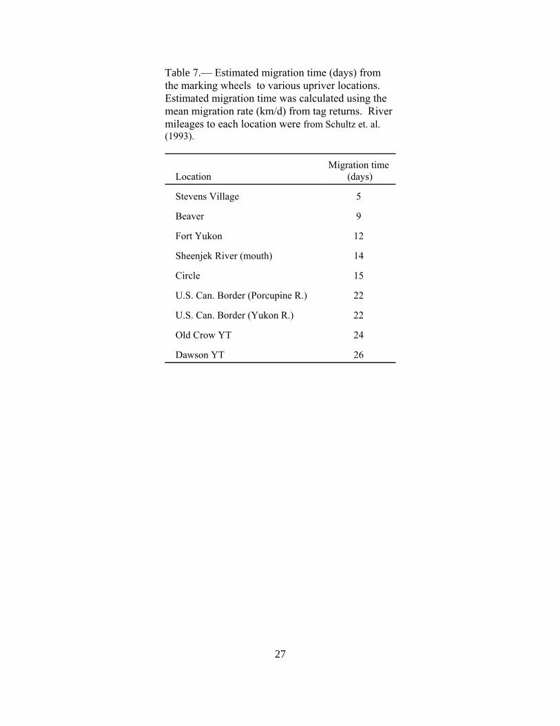
7.— Estimated migration time (days) from the marking wheels to various upriver locations. . 27

8.— Classification of fall chum salmon marked and recaptured in marking wheels on the YukonRiver, Alaska, July 21 to August 11, 1997. . . . . . . . . . . . . . . . . . . . . . . . . . . . . . . . . . . . 28

9.— Consistency of color classification of fall chum salmon marked and recaptured in markingwheels on the Yukon River, Alaska, July 21 to August 11, 1997. . . . . . . . . . . . . . . . . . 29

10.— Results of logistic regressions of capture histories on sex and length, mid-eye to forklength (cm), of fall chum salmon migrating past the marking and recapture wheels on theYukon River, Alaska, July 21 to September 28, 1997. . . . . . . . . . . . . . . . . . . . . . . . . . . 30

11.— Parameter estimates from the logistic regression of capture histories on size, mid-eye tofork length (MEL, cm), and sex of fall chum salmon migrating past the marking andrecapture wheels on the Yukon River, Alaska, July 21 to September 27, 1997. . . . . . . . 31

12 .— River bank capture histories of tagged Yukon River fall chum salmon at the marking andrecapture sites, July 1 to September 24, 1998. . . . . . . . . . . . . . . . . . . . . . . . . . . . . . . . . . 32

13.— Weekly capture histories of tagged fall chum salmon migrating past the marking andrecapture sites on the Yukon River, Alaska, July 20 to September 24, 1997. . . . . . . . . 33

14.— Weekly estimates and those by sex, sex and length, and length. Sampling week are listed

vii

in Table 4. . . . . . . . . . . . . . . . . . . . . . . . . . . . . . . . . . . . . . . . . . . . . . . . . . . . . . . . . . . . . 34

15 .— Weekly population estimates ( ) of fall chum salmon migrating past the marking site onthe Yukon River, Alaska, July 20 to Sep 28, 1997. . . . . . . . . . . . . . . . . . . . . . . . . . . . . . 35

16.— Population estimate ( ) of fall chum salmon migrating past the marking and recapturesites on the Yukon River, Alaska, July 21 to Sept 24, 1998. . . . . . . . . . . . . . . . . . . . . . . 36

17.— Summary of marked to unmarked (percent) at 13 sites distributed through out the YukonRiver drainage upriver from the Rampart Rapids tagging location. . . . . . . . . . . . . . . . . 37

18.— Summary of fish examined for tag loss recorded in 1997 at eightsites in the Yukon River drainage above the Rampart Rapid tagging site from variouslocations of the upper Yukon River. . . . . . . . . . . . . . . . . . . . . . . . . . . . . . . . . . . . . . . . . 38

19 .— Chi-square analysis determined that capture history did not affect (P = 0.07) theprobability of capture at Rampart, Alaska. . . . . . . . . . . . . . . . . . . . . . . . . . . . . . . . . . . . 39

20 .— Chi-square analysis determined that capture history affected (P= 0.001) the probability ofcapture upstream of Rampart, Alaska. . . . . . . . . . . . . . . . . . . . . . . . . . . . . . . . . . . . . . . . 40

21.— Escapement estimates from four projects located upstream from the marking site and totalharvest. . . . . . . . . . . . . . . . . . . . . . . . . . . . . . . . . . . . . . . . . . . . . . . . . . . . . . . . . . . . . . . . 41

viii

List of Figures

1.— Yukon River drainage showing project study sites. . . . . . . . . . . . . . . . . . . . . . . . . . . . . . . 42

2.— Two-basket fish wheel, equipped with padded chute and live holding box, used to collectfish during the marking and recapture events. . . . . . . . . . . . . . . . . . . . . . . . . . . . . . . . . . 43

3.— Estimated migration time (d) for tagged fall chum salmon between the marking andrecapture sites, by statistical week, on the Yukon River, Alaska, July 21 to September 27,1997.. . . . . . . . . . . . . . . . . . . . . . . . . . . . . . . . . . . . . . . . . . . . . . . . . . . . . . . . . . . . . . . . . . . . . 44

4.— Capture probability of two, three, four, and seven day strata plotted by date. . . . . . . . . . 45

5.— Relative abundance CPUE of combined wheel catches versus estimates from 2 d strataDarroch model. . . . . . . . . . . . . . . . . . . . . . . . . . . . . . . . . . . . . . . . . . . . . . . . . . . . . . . . . 46

6— Holding time versus distance (km) to capture of fish harvested in the Yukon River aboveRampart, Alaska. . . . . . . . . . . . . . . . . . . . . . . . . . . . . . . . . . . . . . . . . . . . . . . . . . . . . . . . 47

1

Introduction

In 1985 the governments of the United States and Canada signed a treaty concerningtransboundary Pacific salmon Oncorhynchus spp. (Pacific Salmon Commission 1986). ThePacific Salmon Treaty recognized the unique nature of the Yukon River fishery and directed thePacific Salmon Commission to take steps to clarify the issues and establish a means to managethe fishery cooperatively and equitably (Pacific Salmon Commission 1986). In keeping with thisbroad directive, the governments of Canada and the United States specifically amended thePacific Salmon Treaty in 1995 to address Yukon River issues (Pacific Salmon Commission1995). The amended portion of the Treaty, known as the Interim Agreement, was allowed toexpire in 1998; although, it is still the paradigm under which management agencies currentlyfunction. The Interim Agreement resulted in the formation of an international managementstructure for the Yukon River called the Yukon River Panel (Panel). In 1996, the Panelsupported (in concept) the study described below, to estimate of the number of fall chum salmonin the Yukon River above the confluence of the Tanana River.

The study was originally conceived to ultimately make weekly or bi-weekly populationestimates then apportion those estimates to various drainages in the U.S. and Canada based onradiotelemetry and genetic results. The first step in this study was to determine the feasibility ofconducting a mark-recapture experiment to estimate the abundance of fall chum based oncapture and recapture from fish wheels. Fish wheels have been used successfully on other largerivers as a capture method for tagging studies (Meehan 1961; Merritt and Roberson 1986; Eiler1990;) and for mark-recapture experiments (Greenough 1971; McGregor et al. 1991; Cappielloand Bromaghin 1997). Researchers initiated a project in 1996 on the Yukon River (this study)and established that the mark-recapture model developed by Darroch (1961) could be reasonablyapplied to data collected with fish wheels above Tanana, Alaska (Gordon et al. 1998). The pointestimate produced for 1996 of 654,000 (±41,800) was within 8% of an independent estimatebased on escapement and harvest (Gordon et al. 1998). Precise weekly estimates were alsogenerated and although successful in the initial stages, additional work was needed to gainconfidence in the results.

During 1996 staff identified some potential problems, improvements, and additionalresearch questions that needed to be addressed in the study design (Gordon et al. 1998). Oneproblem was sampling bias at the recapture site precluded stratification based on sex and/orlength. Statistical analysis of 1996 data indicated that stratification by length and sex may benecessary to generate unbiased estimates (Gordon et al. 1998). In 1997, a more rigoroussampling regime was implemented at the recapture site so that stratification by sex and lengthwould be possible. Gordon et al. (1998) also recognized the inconsistencies associated with theassessment of individual fish color and condition as a measure of maturity or “distance” tospawning and the ability to complete the migration, respectively. Better methods were needed tomake these data useful.

Another potential problem was identified in 1996 by cooperators in Canada that revealed recapture to capture ratios (R/C) were extremely low, 0.0008 and 0.0031 at two of escapement

2

projects located on Fishing Branch and mainstem Yukon rivers, respectively. When comparedto the observed ratio of 0.029 for fish handled at the recapture site, the data suggested potentialproblems existed with the sampling methodology that was not detected by statistical analysis. Asecond alternative or implication was that of potential significant mortality caused by oursampling. A number of other hypotheses were identified (Table 1). Actions were taken toinvestigate causes of the anomoly and to more rigorously document R/C values throughout thebasin. One specific action was a thorough examination of tag loss/retention because tag loss wasthought to be a likely explanation.

Directly addressing these problems was necessary to assess potential bias in theestimator used for the computation of weekly and seasonal population estimates. Also, theeffects of sampling protocol changes and results from investigations into the R/C ratios neededto be evaluated before study components of radio telemetry and genetics could be used toapportion the run to specific drainages as originally envisioned (Gordon et al. 1998). Finally, itwas not known if annual variation (e.g., changes in run size) would affect the experiment andevaluation procedures to a significant degree.

The purpose of this study was estimate the annual return of fall chum salmon, to improvethe quality of the estimate, and increase our knowledge in its use. Thus, we repeated theexperiment with the modifications suggested in Gordon et al. (1998) and discussed above.The resulting report, below, documents the changes made in sampling procedures, additionalanalyses of selective sampling and bias, abundance estimates for 1997, and our effort to defineand discover causes behind the reported low R/C ratios.

Study Area

The Yukon River (Figure 1) is the fifth largest drainage in North America, encompassingan area of approximately 855,000 km2 (Bergstrom et al. 1995). Three of the tributaries that jointhe Yukon River are major rivers themselves, each approximately 1,000 km in length. They arethe Koyukuk, Tanana and Porcupine rivers, joining the Yukon at 800, 1,100, and 1,600 km fromthe mouth.

The upper Yukon River, upstream from the Tanana River, is almost 2 km at it widestpoint and flows from about 6-12 km per Two-basket fish wheels (wheels) equipped with paddedchutes and live holding boxes were used to capture chum salmon at the marking site (Figure 2). Wheel baskets at the marking site were approximately 3.0 m wide and dipped to a depth of 4.5 mbelow the water’s surface. Nylon seine netting was installed on the sides of the baskets tominimize injury to fish as they were lifted clear of the water. Closed cell foam padding wasplaced along the chute and ramp on the path to the holding boxes to reduce impact injury to fish. Holding boxes were 2.4 m long, 1.2 m deep, and approximately 1 m wide. The walls and floorsof the holding boxes contained many 5 cm diameter holes to allow a continuous flow of water

3

while preventing heavy current that could potentially impinge weakened fish.

hour. Due to the glacial origins of some of its tributaries the Yukon River is silty during thesummer, but clear during the winter. The region experiences a continental climate with longcold winters and brief warm summers. Air temperatures below freezing are common duringSeptember. The river generally freezes by late October or early November and the ice remainsuntil May of the following year.

Two study sites were maintained on the mainstem of the Yukon River upstream from theTanana River confluence (Figure 1). The location was selected to minimize capture of fall chumsalmon returning to the Tanana River drainage, which constitutes the only major area of fallchum salmon spawning downstream from the study area. The marking site was located at anarea known locally as “The Rapids”, a narrow canyon 1,176 km from the mouth of the YukonRiver. The recapture site was 50 km upstream from the marking site, near the village ofRampart, Alaska.

Methods

Assumptions of the EstimatorThe study was designed as a two event temporally stratified mark-recapture experiment.

We used Darroch’s (1961) model to generate weekly and total estimates of fall chum salmon inthe upper Yukon River. The study design also allowed for stratification by river bank, sex, andlength. Assumptions regarding the application of the Darroch’s model in this study werediscussed by Gordon et al. (1998) and are listed below:

1. Closure: fish in the final stratum must have been present in at least oneinitial stratum.

2. No tag loss: fish must retain their mark and be correctly identified.

3. All fish in a given recapture event, marked and unmarked, have equalprobability of capture.

4. All fish, marked and unmarked, of a given initial stratum have the sameprobability distribution of movement to the recapture strata.

5. Fish captured and marked on the north and south bank mix randomly withrespect to bank orientation between release at the marking site and captureat the recapture site.

Although Darroch’s model allows for spatial and temporal stratification, we had to addassumption 5 because recapture histories of fish marked of north and south banks may belinearly dependent resulting in unrealistic abundance estimates, i.e., those with negative capture

4

probabilities.

One untested assumption remained, that of closure. Examination of closure will dependon radio telemetry data to be provided in 1998 (John Eiler, National Marine Fisheries Service,Auke Bay Laboratory, personal communications). Until these data are available, closure wasassumed because adult salmon migrate upstream from the ocean to spawn, thus pass the markingsite before reaching the recapture site. In addition, a preliminary evaluation of movement to therecapture strata based on 50 radio tagged fish showed minimal (2%) drop back or mortality(John Eiler, National Marine Fisheries Service, Auke Bay Laboratory, personalcommunications).

Marking Site Sampling Procedures

Wheels were placed across from each other on the north and south banks of the river. Wheel placement relative to shore was determined by the depth of the dip on the shoreward edgeof the baskets. This edge was positioned to sweep within 30 cm of the bottom. Wheels weremoved relative to shore as the water level rose or fell to maintain the same proximity to thebottom. A lead, in the form of a submerged picket fence, was placed between the wheel and theshore to direct fish towards the dipping baskets.

Tagging commenced on July 21 and ceased on September 20 at both marking wheels. Fish were marked from Monday through Saturday. Operation of the wheel balanced the need totag approximately 400 fish per day, with the need to spread those tagged fish throughout the day,and the need to minimize holding time. Wheels were run as long as 24 hr per day during timesof low catch rates to fewer than 6 hours on days when catches were high. Generally, crewstagged fish at four different times on most days (usually at 0800, 1200, 1600, and 1900 hrs ADT)and attempted to mark about 100 fish each trip. Wheel operation was minimized to meet the goal of 100 fish per work session. When catch appeared to substantially exceed the goal of 100fish per session, a systematic sample was taken. For example upon arriving at the fish wheel thecrew might estimate that 150 fish were present in the livebox and so every third fish would beexcluded from tagging. Recaptured tagged fish were handled the same as unmarked fish exceptno new length was recorded and no new tag applied. Fish with major injuries (described below)were released. Sub-sampling ended when the live box was emptied even if the goal of 100 fishper work session was exceeded.

Fish were dip netted, handled, and released so as to minimize handling time, stress, andtrauma. Fall chum salmon were marked with individually numbered spaghetti tags applied withhollow applicator needles. We recorded length, sex, tag number, condition and color categories,and release times for all marked fish. Length, mid-eye to fork (MEL), was measured to thenearest cm. Sex determination was based on several external indicators, including the conditionof the kype and teeth, abdominal distention, the size of the adipose fin, and the condition of thevent. Fish with major injuries (as described below) were released untagged and the next fish wasselected.

5

A condition index was developed to determine which fish received tags and as a means totest for behavioral differences that may accompany a fish’s condition. The three conditioncategories were defined as good, minor injury, or major injury (Table 2). All chum salmoncategorized as good and minor injury were tagged.

A color index was developed based upon the degree of spawning coloration or othersecondary spawning characteristics exhibited by individual fish. This index was developed as apossible indicator of distance, either temporal or geographic, to the spawning grounds. Thecategories were defined as silver, light, and dark (Table 3).

Recapture Site Sampling ProceduresThe river at the recapture site was wider and shallower than at the marking site, so the

wheels were sized accordingly. Baskets on the recapture wheels were approximately 2.5 m wideand dipped to a depth of 3.0 m below the water’s surface. The south bank wheel was placedabout 2 km downstream from the north bank wheel.

Recapture procedures carried our by a contractor and discussed below included: 1)recording marked and unmarked fish; 2) sub-sampling for sex and length data designed to allowstratification of the estimate; and 3) sub-sampling designed to estimate tag loss. First, fish werechecked for primary marks while in the dip net, marked and unmarked fish tallied, tag numbersand release times were recorded, and the fish released. Fish escaping capture prior to the tagbeing read were recorded as such and assigned to a statistical week of marking based on theproportion of weeks from the identified tags. Second, length, sex, condition, and color wererecorded from a sub-sample of approximately 150 fish per statistical week. The fish werecollected so that the data were spaced throughout the week on at least three days (e.g., Monday,Wednesday and Friday, fifty fish from each day). When a day was selected for sampling, auniform sub-sample was taken from each live box. For example, data were collected from everyeleventh fish until the box was empty. The integer used for sample selection was based on theprevious days catch divided by 50 and then rounded down. When the target number was reachedprior to emptying the live box, the sub-sampling was not stopped until the live box was emptied. Finally, a second sub-sample was taken to examine tag loss in a sub-sample of 100 fish per day(approximately) from the first live boxes emptied. These fish were examined for the presence ofprimary and secondary marks. When high densities of fish were encountered, the sub-sampleused a uniform sampling regime to reduce the number of fish handled (e.g., examined everythird fish). Three tallies were recorded: (1) the total number of fish examined in the sub-sample,(2) fish with primary and secondary marks, and the (3) fish with only a secondary mark. Again,the sub-sample was not stopped until the live box was empty.

Sampling commenced at both recapture wheels on July 22 and ceased on September 28. Recapture wheels were operated 24 hours a day, seven days a week. The frequency of emptyingfish from the box depended on the density encountered; the holding box was emptied at leastfour times per day on most days. The contractor was instructed to make every effort to maintainthe live box so that the number of fish never exceeded 200 fish.

6

Analysis of Tagging and Recovery Wheel DataMigration times.— Migration times were calculated for all fish tagged and released at the

marking wheels and caught 50 km upstream in the recapture wheels. Migration time for eachrecaptured fish was calculated as follows.

(1)

wherer = date and time, to nearest minute, of a marked fish’s release at the

recapture wheels,

g = date and time, to nearest minute, of the beginning of a samplingperiod at the recapture wheels, and

d = migration start time, date and time, to nearest minute, of a markedfish’s release at the marking wheels.

Since we did not know the exact time of day that fish were caught in the recapture wheels themidpoint of r and g, i.e., (r ! g)/2, was used to calculate the migration end time.

Migration times were also calculated for tags returned by upriver fishermen and DFOfisheries projects. Tags that were accompanied with dates and location of harvest were used tocalculate migration times and migration rates. Migration rates were calculated as the distance inriver km (Schultz et. al. 1993) from the tagging site to the recapture site, divided by migrationtime. Migration times were calculated to the nearest day (1200 hr as a midpoint) because oftenonly the day and not the time of recapture was available.

Tag retention.— Data on the presence of primary and secondary marks from fishrecaptured at the recapture site were used to estimate tag retention (tag loss) between themarking and recapture sites. During sub-sampling at the recapture fish wheels (described above)tallies were collected of total fish examined, fish with primary and secondary marks, and fishwith only secondary marks.

Assessment of condition and color classifications.— An assessment of the crew’s abilityto classify fish by condition and color (Table 2 and 3) was conducted in light of inaccuraciesdescribed in by Gordon et al. (1998). Using fish that were tagged, released, and recaptured atthe marking wheels, the condition and color classification data were examined for consistencybetween the first and second examinations.

Equal probability of capture and movement to recapture strata.— Tests could not bedeveloped to determine if (1) all fish had an equal probability of capture at the recapture site or

7

(2)

(2) if all fish had the same probability distribution of movement between marking and recapturewheels. Instead we determined if the recapture probabilities, Darroch’s Rij’s (i.e., the productof probability of movement to recapture strata, 2ij, and capture probabilities, pj) were the samefor all marked fish of release stratum i. Given that

where

cij = number of marked fish released during week i that were recaptured for thefirst time during week j (the implicit and untestable assumption is thatmarked and unmarked fish behaved similarly),

andai = number of marked fish released during the ith week at the marking site,

we were able to use the recapture data to perform this analysis.

Multinomial logistic regression, using generalized logits (Agresti 1990) was used tomodel the probability of recapture as a function of a fish’s sex and length. In choosing a model,a likelihood-ratio test was compared the fitted model with a simpler one and then removedparameters one by one until it was determined that the fitted model added significant explanatoryvalue over the simpler one. The process was started by comparing the full model, i.e., onecontaining the effects of sex, length, and their interaction, with an intercept-only model. Themodel selection process continued only if the full model was chosen over the intercept onlymodel, i.e., if the likelihood-ratio test statistic, G2 (full | intercept only), was significant (P #0.05). Next a comparison was made between the full model and the main effects model, i.e., onecontaining sex and size. If the test statistic was significant then the main effects model wascompared to the best fitting single effect model, i.e., one containing sex or size.

Data collected at the marking and recapture sites were grouped into statistical weeks(Table 4). At the marking site statistical weeks began on Monday and ended on Saturday. Atthe recapture site statistical weeks began on Tuesday and ended on Monday to allow formigration time from the marking site. Separate analyses were performed for each markingweek, i.e. stratum.

Random mixing.— Following Agresti (1990, section 7.4.1), we used a log-linear modelto test if north and south bank marked fish had randomly mixed at the recapture sites. Wecombined data from marking weeks to increase power, but controlled for the effect of thestratum. Combining the data and performing simple 2-factor tests of independence would haveled to improper weighting of the data and possibly erroneous conclusions (Christensen 1990). Performing this log-linear analysis, conditioned on statistical week, is analogous to performingthe Cochran-Mantel-Haenszel Test (Agresti 1990).

8

$ ' ,n b C a= −1 (4)

$

''

c c uc

cij ij j

ij

i ji

n= +

=∑

1

(5)

Abundance estimate.— Following Darroch (1961), the estimate of the number of unmarked fish migrating through our study area, , was estimated by$n

where

a = a vector with elements ai, the number of tagged fish released in stratum i;

C = a matrix with elements cij, the number of tagged fish released in stratum ithat were recaptured at the recovery site during recovery week j; and

b = a vector with elements bj, the number of untagged fish captured at therecovery site during recovery stratum j.

With four exceptions, we followed the same procedures used by Gordon et al. (1998) forestimating weekly and total abundance, their variances, and statistical bias. First, we had toestimate the elements of C because 24 fish were recaptured but their tag numbers were notrecorded. Although we knew when these fish were recaptured, we did not know when they weretagged. Consequently, we estimated the number of fish tagged in stratum i and recaptured inrecovery stratum j where:

Wherecij = the known number of fish tagged in stratum i and recaptured in recovery

stratum j, anduj = the number of fish recaptured in recovery stratum j with unknown tag

numbers.Second, because we wanted to generate separate abundance estimates for male and female fishand for different length classes of fish, but because we recorded the sex and length of only asample of untagged fish captured at the recovery site, we had to estimate uj. We did this simplyby multiplying uj by the proportion of fish of a given sex and length class in the sample takenduring stratum j.

Third, based on the distribution of travel times, we assumed that some of the untaggedfish captured in recovery wheels during the first week of the study, passed the tagging site beforethe start of the experiment. This violates the assumption of closure; if true and left uncorrectedwould bias our estimates upwards. Thus, we used data from the second and third weeks of thestudy, and the methods used by Cappiello and Bruden (1997) to estimate the proportions ofunmarked fish that passed the marking site after the study began, and that were captured in the

9

recovery wheels upstream during the first week of the study, to correct these numbers (Table 5). The implicit assumption being that marked and unmarked fish travel between marking andrecapture sites at the same rate. Similarly, we had to adjust downward the number of fishmarked and released during the last week of the study because some of them did not pass therecovery site until after the study was completed (Table 6). Lastly, we generated abundanceestimates for 2, 3, 5, and 7-day intervals, as well as for the whole season.

CPUE versus estimated abundance.— Relative abundance was measured by the catch perunit effort (CPUE), number of fish in a 24 h period. At the marking site the amount of time thewheel fished varied from 24 h to less than 6 h per d so catches were expanded to 24 h. At therecapture site wheels were run 24 h per d so no expansion was necessary. Marking and recapturewheel CPUE plotted by date were compared to corresponding abundance estimates. CumulativeCPUE date and corresponding cumulative abundance estimates were also plotted by date.

Analysis of Recapture to Capture Ratios Nine hypotheses (Table 1) were developed to explain and test why recapture to capture

ratios (R/C) would be lower in upper basin areas than those found at our recovery wheels atRampart, Alaska. Five hypotheses were addressed by protocol changes or specific effort tocollect the data needed to evaluate each as discussed below (Table 1, incomplete reporting, #1 ;dilution from immigration of the unmarked tails of the run, # 2; tag loss # 3; selective samplingfor or against one stock # 4; and induced mortality # 8). The remaining hypotheses 5 - 7 and 9 ofTable 1 were not addressed in 1997.

Incomplete reporting.— The possibility of incomplete reporting was reduced by targetingdata collection designed specifically to address this problem. In 1996, R/C data were availablefrom two sources in Canada and were collected incidental to work during other projects. Incontrast in 1997, people were trained to collect data at eight locations upstream of the recapturesite specifically to provide R/C estimates. Additional data were also collected from subsistencefishers. Data received included tallies of total catch and number of fish with primary marks.

Immigration of unmarked fish.— In 1996 tagging began on August 1 reportedly after thefirst group of fall chum salmon passed the marking site and ended while the run was still fairlystrong based on the estimate of fish passage the last week (Gordon et al. 1998). Thesecircumstances may have allowed large numbers of unmarked fish to pass the marking sitewithout being exposed to sampling, thereby effectively reducing the proportion of tagged fish upstream. To correct this problem, sampling began approximately ten days earlier in 1997. Inaddition, we monitored catch per unit effort and examined the estimate of the last week oftagging to determine whether or not fish passage had tapered off during the last week. By theseactions, the effect caused by the immigration of unmarked fish was reduced or at leastpurposefully monitored.

Tag loss.— The addition of a secondary mark to all tagged fish during the processingprotocol allowed us to examine tag loss in upstream areas. Trained individuals at the eightlocations (as mentioned above) sampled catches of subsistence and commercial fishers, and

10

research projects. They recorded total catch, fish with primary marks, and fish with onlysecondary marks.

Selective sampling.— Selective sampling can occur in two ways. First, a portion of allstocks is unavailable for sampling (based on sex or length, which were described above, oranother characteristic not identified). Second, an individual stock or stocks are unavailable forsampling. We examined the second of these possibilities. Testing the hypothesis of selectivesampling for one or more stocks beyond our recapture site required R/C ratios to be collectedfrom all known spawning stocks. If a number of stocks had R/C ratios far below the seasonalaverage and this was based on stock specific sampling, then one could reason that somewhereelse in the drainage one or more stock must have R/C ratios higher than the seasonal average. The collection of data on most spawning stocks was incidental to the sampling described above;however, special efforts had to be directed towards two additional spawning areas, the Chandalarand Sheenjek rivers. Carcass surveys were conducted on these rivers during two days inOctober, 1997. Data recorded included location, total number of fish examined, total number offish with primary or secondary marks, and tag numbers if present.

Effects of repeated capture.— The effect of handling fish was examined by comparingthe probabilities of capture upstream. Two chi square tests were conducted that examined theprobability of tag recovery after various capture histories using a 2×4 contingency table. Thecontingency tables were used to examine counts of recaptured fish versus fish not recapturedsubsequent to one, two, three, or more than three capture and release experiences. The first testexamined fish capture histories at the marking site versus fish subsequently caught at therecapture site at Rampart, Alaska. The second test included fish capture histories at both themarking and recapture sites versus fish final recovery upstream of Rampart, Alaska.

A second examination of the effect of repeated capture focused on cumulative holdingtimes during processing. Cumulative holding time, an estimate of the total time spent in the livebox at the four wheels, was calculated by summing all holding times a fish experienced. Holding time was calculated as follows:

(5)

wherer = date and time, to nearest minute, of a marked fish’s release at a

wheel,

g = date and time, to nearest minute, of the beginning of a samplingperiod at a wheel.

Cumulative holding time was plotted against the distance to final capture.

11

Results

Analysis of Tagging and Recovery Wheel DataFrom July 21 through September 20, 1997, 18,631 fall chum salmon were tagged at the

marking wheels. Lengths of tagged fish ranged from 47 to 73 cm MEL. Males made up 48%and females 52% of the tagged fish. Holding times during tagging ranged from 0.05 to 18.4 hwith the mean, median, and mode holding times of 4.3, 3.5, and 3.2 h, respectively. From July22 to September 22, 40,978 fall chum salmon were examined for primary marks at the recapturesites. Excluding multiple recaptures, 1,872 marked fish were recaptured. On average fewer than5% of the fish were recaptured more than once at the recapture site.

Migration times.— Modal estimated migration time between the marking and recapturewheel for tagged fish was 2 d or less in each statistical week (Figure 3). Estimated migrationtimes for individual tagged fish ranged from less than 1 d in week 7 to 40 d in week 1. Variationin estimated migration time decreased from statistical week 1 to 9. Approximately 90% oftagged fish released during week 1 took 4 d or less to reach the recapture wheels. In week 9approximately 90% of the tagged fish released took 2 d or less to reach the recapture wheel.

Approximately 1,050 tags were returned by subsistence and commercial fishersthroughout the Yukon River drainage. Of these 989 were returned from upriver of the tagginglocation. Tags were returned from locations greater then 1,300 kilometers upriver of the taggingsite including the Kluane and the Fishing Branch Rivers in Canada. Tags were returned from asfar down river as the village of Kaltag, 452 k away.

Migration rates were calculated for 379 tagged fish that were harvested in upriverfisheries, or captured by DFO fisheries projects. The mean migration rate of harvested taggedfish was 36 km/d (SE = 0.5) with a range of 16 to 111 km/d. The mean migration rate from themarking wheels to the recapture wheels near Rampart was 30.3 km/d. The mean migration rateof 36 km/d was used to estimate migration time in days from the marking wheels to differentlocations upriver (Table 7).

Tag retention.— No evidence of tag loss was observed. A total of 9,697 fall chumsalmon were examined at the recovery wheels at Rampart, Alaska. Of the 575 fish found withfin clips none were observed to have lost their primary mark, the spaghetti tag.

Assessment of condition and color classifications.— Classification between the mark andsecond assessment was inconsistent for condition and color in the fish sampled in the first threeweeks of sampling (n = 908). For condition, 13 and 44% were reclassified differently uponrecapture for the good and minor injury categories, respectively (Table 8). For color, 67, 14, and31% were reclassified incorrectly for the silver, light, and dark categories, respectively (Table 9). Based on these data condition and color data were not collected after August 11 and wereeliminated from further analysis.

Equal probability of capture and movement to recapture strata.— Violations of theassumption of the equal probability of recapture were noted, but appeared to have little effect on

12

the estimate. Differences between the full model and that model with just the intercept (Table10) indicated that sex and length or the interaction variable helped predict recapture in statisticalweeks 3 (P = 0.05) and 8 (P = 0.01). Further analysis of those two weeks using the full andmain effects model indicated the interaction between size and sex helped predict recapture inweek 3. No significant interaction was detected for week 8 allowing the interaction term to bedropped. Analysis of the best single effect, length and sex had similar results, no effect, whenanalyzed with the main effect model, but significant effect with the intercept model. Values forG2 were higher for length than for sex, G2 = 8.4 versus G2 = 6.9, respectively, but both variablesexplained more variation in recapture than the intercept only model. Parameters estimates arepresented in Table 11. The results indicated that stratification by sex and/or length may reducebias of the weekly estimates.

Random mixing.— Marked fish randomly mixed between release at the marking site andrecapture at the north and south bank recapture wheels (Table 12, G2 = 11.40, P = 0.18). Nointeraction between banks and weeks was detected (G2 = 4.92, P = 0.67). In addition, once theinteraction term was dropped no main effects were significant. Interpreted as a indication ofrandom mixing, the data indicated that no stratification of the estimate by bank is required.

Abundance estimates.— Tabulated data (Table 13) were used to generate weekly andseasonal estimates as well as those estimates further stratified by sex and length (Table 14). Theseasonal estimate was not significantly different than estimates stratified by sex, sex and length,and length. The estimates based on further stratification were within 2.5% of the correspondingbootstrap result (Table 15). The similar results indicated that bias based on sex or length isnegligible, supporting the statistical analyses above.

Estimates were also generated using alternative temporal strata, two, three, four d inaddition to the seven d strata described above (Table 16). Temporal strata at the marking andrecapture sites were changed in unison. These estimates were similar to each other and indicatedthat the estimate is robust to changes in capture probabilities based on the selection of theduration of the temporal stratification. Confidence intervals for the shorter time periods werewider than for estimates with longer time periods because finer stratification increases thenumber of parameters being estimated and reduces sample size within the strata. Probability ofcapture within a strata varied more widely in 2 d strata than in longer strata (Figure 4).

CPUE versus estimated abundance.— Marking and recapture wheel CPUE plotted bydate were compared to corresponding abundance estimates (Figure 5). The measures of relativeabundance tracked well except that Darroch estimates tends to lead CPUE in time and indicatefuture direction regarding increases and decreases. In a few instances the estimate and CPUEdisassociated, for example July 22 and August 18. Also, an individual wheels CPUE andestimated abundance were more likely to disassociate than the combined CPUE total from twowheels.

Analysis of Recapture to Capture RatiosThe R/C ratios based on tag recovery at 13 sites upstream of the recapture wheel

13

indicated an inverse relationship with distance (Table 17). Using these data, several of thepotential explanations for observed low R/C ratios were examined directly and by inference.

Incomplete reporting.— Incomplete reporting was addressed by designing a plannedeffort to gather data from upstream areas and training personnel in recognizing primary andsecondary marks on fish. No change in the relationship (R/C vs. distance) between 1996 and1997 was observed by adding to the number of observations. For example, the change in R/Cvalues between the recapture wheels at Rampart, Alaska, and the DFO fish wheels located on theYukon River mainstem near the border was a decrease by 80%.

Immigration of unmarked fish.— Tagging was initiated on July 21, two weeks earlierthan during 1996 and continued until September 20 when the run had substantially declined. The final weekly estimate in September declined to 21,800 fish per week (5% of the totalestimate in 1997) from 39,500 fish the previous week. In addition, CPUE declined from 397fish/ 24h on September 13 to 171 fish / 24 h on September 20 in a steady decline. In contrast,final weekly estimates during 1996 remained over 69,000 fall chum salmon or 10% of the totalestimate in 1996(Gordon et al. 1998).

Tag loss.— Tag loss was specifically examined at eight sites ranging from 52 to 1402 km upstream of the tagging location. No fish were found to have lost their primary mark at theselocations (Table 18). Fish were collected throughout the season at two of the sampling locations,while at the other sites fish were sampled over shorter time segments.

Selective sampling.— Mis-allocation of tags by over or under representing one or morestocks was examined by collecting data representing all known major spawning areas. The R/Cvalues listed (Table 17) do not indicate values higher than the proportion found at the recapturesite of 5.0 % with one exception where the sample size was low.

Effects of repeated capture.— A history of repeated capture at the tagging wheels wasfound not to affect the probability of recapture (O 2 = 6.93, d.f. = 3, and P = 0.07) when the finalcapture was at the recovery site at Rampart, Alaska (Table 19). In contrast, when the recapturehistories included repeated captures at all wheels versus final capture upstream from therecovery site, the probability of recapture differed significantly from their expected values (O 2 =36.04, d.f. = 3, and P = 0.001); fish captured two or three times were half as likely to berecaptured upriver (Table 20).

Plots of total holding time in the fish wheel live box vs distance to final capture offeredno additional insight to explain the low R/C ratios upstream (Figure 6). Total holding times forfish with one or more captures ranged from less than 1 h to 44 h with a mode of 3.15 h andmedian of 3.77 h.

14

Discussion

The ability to obtain precise weekly estimates from a major sub-basin of the Yukon Riverpresents unique opportunities to learn about the spawning stocks and potentially, to managefisheries upstream more effectively. The weekly population estimates investigated here could be an important index for the sub-basin, but equally important they provide a platform for othertechniques to exploit, for example, radiotelemetry and genetic analysis. Radiotelemetry cantrack salmon to individual drainages with 99% reliability (Eiler 1995) allowing the potential ofweekly estimates that could be partitioned by drainage. Radiotelemetry also provides the abilityto identify as yet unrecognized spawning areas (Eiler et al. 1992). Genetic analysis also holdgreat potential to exploit the information generated by the weekly estimates given a significantbreakthrough regarding genetic markers needed to separate upriver stocks (Beecham et al. 1988;Wilmot et al. 1992; Wilmot et al. 1994). Genetic sampling during the mark and recaptureprogram could provide percentage stock composition by week through a mixed stock analysis. Inseason analysis of stock composition as the run travels through Alaska could give Canadianfishery managers a picture of the stocks that will be available for harvest that much earlier and substantially more accurately than is now available.

Potential benefits described above depend heavily on the accuracy and precision of theestimate. Data collection in 1997 improved our confidence in the abundance estimates in mostaspects while identifying the need for investigation of a few other areas. Much of the additionaleffort focused on the assumptions require for use of the estimator. For example, the assumptionof tag retention is important and has received insufficient attention (Seber 1982). Significanttag loss could add bias to weekly and seasonal estimates. In addition, tag loss was one possibleexplanation of the low R/C ratios found upriver. Thorough investigation of tag retention/loss atthe recovery site 52 km upstream revealed that no tag loss was observed and the assumption wasmet. In addition, no fish processed two or more times at the marking wheel were found to havelost a tag. This makes sense because time and distance between mark and recapture are minimalcompared to studies where recapture occurs on distant spawning grounds. In comparison, thepotential for tag loss in this study is minimized. Finally, tag loss was not found in upstreamareas despite extensive effort. These findings are similar to those reported for fall-run chumsalmon (Cappiello and Bromaghin 1997; Cappiello and Bruden 1997) from the Tanana River, atributary of the Yukon River.

Mortality or downstream movement of tagged fish would violate the assumption ofclosure. Others researchers have included a correction for mortality of 5 to 10% (Milligan et al. 1986; Cappiello and Bromaghin 1997). Gordon et al. (1998) did not use a correction becausethe data available from radio telemetry indicated correction was unwarranted. In 1996, of fiftyradio tagged fish released at the tagging site 48 fish moved passed a tower 11 km above therelease site, one fish regurgitated its tag after recapture at the marking site, and one fish was notrelocated (John Eiler, National Marine Fisheries Service, Auke Bay, personal communication). No fall chum salmon spawning areas are known to occur between the marking and recapturesites.

15

The mean migration rate of 36 km/d, based on travel between the marking and recoveryfish wheels, was higher than the mean migration rate of 26 km/d reported by Cappiello andBromaghin (1997) for fall chum salmon in the upper Tanana River. However, similar migrationrates have been reported by others. Milligan et. al. (1986) reported average migration rates of30.5 - 35.7 km/d for chum salmon during a mark-recapture study, and an average rate of 37.9during a telemetry study in the upper Yukon River in Canada. Buklis and Barton (1984) alsoestimated a similar migration rate of 37 km/d in the lower Yukon by comparing mean date ofpassage between different test fishing sites.

The assessment of condition and color continued to be plagued by inconsistency despiteapriori definitions for each category and efforts to train crew members, as suggested by Gordonet al. (1998). The categories were to be used to evaluate the temporal or spatial distance fromspawning. Part of the problem is that the technicians must evaluate multiple continuous traits toassign each fish to a category. These traits do not vary consistently with each other. Forexample, one fish may be fully scaled, silver, and have a developed kype; the next fish may haveabsorbed scales, be yellow, and have little kype development. The result is opposing indicationof maturity or “closeness” to spawning. Alternatively, fisherman told us that fish change colorin the live box although we had no way to quantitatively test this hypothesis. As in1996 (Gordonet al. 1998), attempts to use these categories were ended.

Analysis of probability of recapture data suggested some evidence that bias in samplingoccurred. Statistical analysis revealed limited violations of the assumptions of probability ofrecapture based on length and sex for a second year row. The similarity of results betweenyears adds some confidence in the procedure; however, the statistical analyses of bias describedabove falls short of ideal because of the inseparable association of the probabilities of captureand movement (Seber 1982), Darrochs’s Rij’s (i.e., the product of probability of movement torecovery strata, 2ij, and capture probabilities, pj). These associated probabilities could varywithin Rij, in essence canceling each other out while change in the overall value remainsnonsignificant. Modeling presented by Gordon et al. (1998) showed that the potential forsubstantial bias was small if 2ij varies, but if pj varies, the bias can be large. Therefore, onecannot be certain that bias is small despite the statistical tests. In view of the finding of limitedviolations regarding sex and length found in both years (Gordon et al. 1998; this study), one cansee the need to further investigate any indication of a potential for bias thus highlighting thenecessity of having the ability to stratify by length and sex.

The advantage gained in 1997 by the ability to stratify by sex and length becomesapparent when stratification is used to reduce any bias based on those characteristics. When theseasonal estimate was compared to the seasonal estimate generated by stratifying by sex and/orlength, the estimates were quite similar indicating bias was negligible. In contrast, inadequatedata in 1996 required Gordon et al. (1998) to model the potential effects of bias, with theconclusion that bias was likely to be small. The addition of the 1997 data supported thehypothesis of Gordon et al. (1998) that violations measured statistically are likely due todifferential movement between temporal strata rather than size or sex based selective sampling.

16

Similarly, the length of the temporal strata used had little effect on the estimates. Temporal strata duration was manipulated to produce estimates based on two, three, four, andseven d strata length (Table 16). Despite the constantly changing probability of recapture(Figure 4), in apparent violation of the assumption of constant probability of capture, our dataappear robust to the need of constant wheel efficiency within a stratum. The various estimateshave different strata length, but the results were similar.

As in 1996, the estimate generated from mark-recapture data compared favorably with anindependent estimate compiled from escapement and harvest data. Estimates of fall chumsalmon escapement unrelated to this study are made in four portions of the Yukon Riverdrainage. Escapement estimates from these four locations, plus harvest between the TananaRiver and the location of escapement, can be used as an alternate minimum estimate of fall chumsalmon (Table 21). The project data used represent the majority of the known spawning stocksand harvest in the Yukon River drainage above the Tanana River. Our 1996 estimate was low byapproximately 8%; 654,296 versus 708,812 fish of the independent estimate. Our 1997 estimatewas low by 15%; 369,547 versus 430,493 fish. The consistent difference, our estimate beingless, compared to the other escapement projects may or may not be significant. The potentialcause remains unclear, but further work on the issue should be a focus for additional study.

Recapture to capture ratios reported from Canada in 1996 needed further investigationbecause two hypotheses (Table 1, #4 and 5) suggests a potential for bias in the run estimate andanother suggests substantial mortality caused by handling fish. Several potential hypotheses forlow R/C were addressed in 1997. Incomplete reporting, and immigration of unmarked fish wereaddressed with changes in procedure. Those procedural changes had no effect on the trend ofdecreasing R/C ratios upstream observed in 1997 which was similar to that found in 1996. Tagloss also appears to be negligible even into the upper Yukon River Basin. Observations of R/Cratios representing the various spawning stocks and drainages are less robust, but still add to thepicture. Among the drainages no observations indicated over-represented stock that mightbalance the low values found in most areas. To reasonably explain the low R/C values based onmis-allocation to one or more stocks, somewhere within the drainage, R/C values higher than theseasonal average would need to be observed. Although large number of fish were examined,carcass surveys were considered only a “snap shot” of the true R/C ratio for the drainage. Noobservations were gathered in the Black River drainage, thought to be a minor spawningtributary, and the possibility of mainstem spawning remains; however, the data available indicatereduced R/C ratios occur drainage wide. This analysis only examined mis-allocation based onstock. A remaining possible hypothesis of mis-allocation (Table 1, Hypothesis #5) based onfactors other than stock (length, sex, migration path, etc.) needs to be kept separate because theanalysis requires different data.

One additional hypothesis was examined using the 1997 data, that of differentialmortality between marked and unmarked fish (Table 1, #8). Repeated captures did have aneffect on the probability of recovery upstream of Rampart, but did not affect the probability ofrecapture at Rampart where results of the recovery strata for the Darroch estimator were tallied. Thus we conclude that the mortality was delayed at least several days. We also conclude that

17

some mortality is associated with the processing of fish. The implication of induced mortality issignificant because not only does the current project handle over 60,000 fish in some years, butseveral other test wheels are being used to gather management data throughout the Yukon River. Mortality caused by these studies needs to be carefully investigated and should be a highpriority.

Handling caused stress and resulting mortality in fish are well documented (Stichney1983; Adams 1990; Wedemeyer 1990). The mortality caused by handling can be delayed(Stichney 1983) and the effects cumulative (Wedemeyer 1990) which fit well to explain theobserved R/C ratios found upriver. Direct investigations into fish wheel stress and morbidityhave not been well documented. Possible causes of elevated stress include physical capture bythe wheels, holding time in the live box, crowded conditions within the live box, handlingprocedures, and tagging. Given the popularity of fish wheel CPUE as a monitoring tool, itappears prudent to investigate possible ill effects further. Investigation into each possible causemay lead to changes in procedures that would eliminate mortality (though not yet proved) orreduce it to an acceptable level.

Conclusions

Data collected in 1997 substantially advanced our knowledge about the use of theDarroch estimator to estimate the number of fall chum salmon migrating in the Yukon Riverabove the confluence of the Tanana River. We concluded that bias based on violations of equalprobability of recapture based on sex and length were negligible. Some questions remain, e.g.,explaining the phenomena of progressively lower R/C ratios in the drainage above the recoverysite. Several hypotheses remain to be tested regarding this question and these should beinvestigated further. In addition, some question remains regarding difference between ourestimate and that based on harvest and escapements. However, the preponderance of our dataindicated that precise and credible estimates can be generated from varying run sizes of fallchum salmon. Furthermore, genetic analysis and radio telemetry can be added to the projectwith reasonable hope that the weekly estimates can be partitioned into sub-basins.

Acknowledgments

We would like to recognize the contribution of the seasonal technicians, J. Moreland, P.Anselmo, R. Morris, and J. Tilley. Numerous other individuals provided assistance in fieldoperations including L. Devany, K. Russel, B. Spearman, S. Murley, D. Pearson, Leslie Reiz, K.Holland, and M. Gendron. We thank M. Millard, R. Simmons, and K. Kimbrel for theirsupervisory and administrative oversight. S. Zuray and P. Evans operated and maintained thefish wheels for us and did and excellent job. Refuge Information Specialist P. Williams ofBeaver and A. Peters resident of Fort Yukon provided data on recapture rates from the FortYukon area. We thank I. Boyce from DFO Canada for providing data from Yukon Territory. For external review we thank C. Krueger, J. Eiler, J. Pella, and J. Bromaghin

18

References

Adams, S. M., editor. 1990. Biological indicators of stress in fish. American Fisheries SocietySymposium 8.

Agresti, A. 1990. Categorical data analysis. John Wiley & Sons, Inc., New York.

Beacham, T. D., C. B. Murray, and R. E. Withler. 1988. Age, morphology, developmentalbiology, and biochemical genetic variation of Yukon River fall chum salmon,Oncorhynchus keta, and comparisons with British Columbia populations. FisheryBulletin, Volume 86, Number 4.

Bergstrom, D. J. and six coauthors. 1995. Annual management report Yukon area, 1993. Alaska Department of Fish and Game. Regional Information Report No. 3A95-10. Anchorage, Alaska.

Buklis, L. S. 1981. Yukon and Tanana river fall chum salmon tagging study, 1976-1980. Alaska Department of Fish and Game. Information Leaflet Number 194.

Buklis, L. S. and L. H. Barton. 1984. Yukon River fall chum salmon biology and stockstatus. Alaska Department of Fish and Game. Information Leaflet Number 239.

Busher, W. 1997. Commercial fin fish harvest statistics for the upper Yukon and Northern management areas, 1996. Regional Informational Report No. 3A97-11. Alaska Department of Fish and Game. Anchorage, Alaska.

Cappiello, T. A., and J. F. Bromaghin. 1997. Mark-recapture abundance estimate of fall-runchum salmon in the Upper Tanana River, Alaska, 1995. Alaska Fishery ResearchBulletin 4(1):12-35.

Cappiello, T. A., and D. L. Bruden. 1997. Mark-recapture abundance estimate of fall-run chumsalmon in the Upper Tanana River, Alaska, 1996. Alaska Department of Fish and Game,Anchorages, Regional Information Report No.3A97-37.

Christensen, R. 1990. Log-linear models. Springer-Verlag, Inc. New York.

Darroch, J. N. 1961. The two-sample capture-recapture census when tagging and sampling arestratified. Biometrika 48:241-260.

Eiler, J. H. 1990. Radio transmitters used to study salmon in glacial rivers. American FisheriesSociety Symposium 7:364-369.

Eiler, J. H. 1995. A remote satellite-linked tracking system for studying pacific salmon withradio telemetry. Transactions of the American Fisheries Society 124:184-193.

19

Eiler, J. H., B. D. Nelson, and R. F. Bradshaw. 1992. Riverine spawning by sockeye salmon inthe Taku River, Alaska and British Columbia. Transactions of the American FisheriesSociety 121:701-708.

Gordon, J. A., S. P. Klosiewski, T. J. Underwood, and R. J. Brown. 1998. Estimated abundanceof adult fall chum salmon in the upper Yukon River, Alaska, 1996. U. S. Fish andWildlife Service, Fairbanks Fishery Resource Office, Alaska Fisheries Technical ReportNumber 45, Fairbanks, Alaska.

Greenough, J. W. 1971. Estimation of sockeye, coho, and chinook salmon runs at WoodCanyon on the Copper River in 1966, 1967, and 1968. Final Report from the NationalMarine Fisheries Service, Auke Bay Coastal Fisheries Research Center, Auke Bay,Juneau, Alaska.

McGregor, A. J., P. A. Milligan, and J. E. Clark. 1991. Adult mark-recapture studies of Taku River salmon stocks in 1989. Alaska Department of Fish and Game, TechnicalFishery Report 91-05.

Meehan, W. R. 1961. Use of a fishwheel in salmon research and management. Transactions ofthe American Fisheries Society 90: 490-494.

Merritt, M. F., and K. Roberson. 1986. Migratory timing of upper Copper River sockey salmonstocks and its implications for the regulation of the commercial fishery. North AmericanJournal of Fisheries Management 6:216-225.

Milligan, P. A., W. O. Rublee, D. D. Cornett, and R. A. C. Johnston. 1986. The distribution andabundance of chum salmon Oncorhynchus keta in the upper Yukon River basin asdetermined by a radio-tagging and spaghetti tagging program: 1982-1983. CanadianTechnical Report of Fisheries and Aquatic Sciences 1351:141 p.

Pacific Salmon Commission. 1986. First annual report 1985/86. Vancouver, BritishColumbia, Canada.

Pacific Salmon Commission. 1995. First annual report 1994/95. Vancouver, BritishColumbia, Canada.

Schultz K.C., and six others. 1993. Annual management report for subsistence, personal use, andcommercial fisheries of the Yukon area, 1992. Alaska Department of Fish and Game, Division ofCommercial Fisheries. Regional Information Report No 3A93-10. Anchorage.

Seber, G. A. F. 1982. The estimation of animal abundance and related parameters. 2ndedition. Charles Griffin & Company, London.

Stichney R. R. 1983. Care and handling of live fish. Pages 85-94 in L. A. Nielson and D. L.Johnson, editors. Fisheries Techniques. American Fisheries Society, Bethesda,

20

Maryland.

Wedemeyer, G. A., B. A. Barton, and D. J. McLeay. 1990. Stress and acclimation. Pages 451-490 in C. B. Schreck and P. B. Moyle, editors. Methods for fish biology. AmericanFisheries Society, Bethesda, Maryland.

Wilmot, R. L., R. Everett, W. J. Spearman, and R. Baccus. 1992. Genetic stock identification ofYukon River chum and chinook salmon 1987 to 1990. Progress Report. Alaska Fish andWildlife Research Center, Fisheries Management Services, U.S. Fish and WildlifeService. Anchorage, Alaska.

Wilmot, R. L., R. J. Everett, W. J. Spearman, R. Baccus, N. V. Varnavskaya, and S. V. Putivkin. 1994. Genetic stock structure of western Alaska chum salmon and a comparison withRussian Far East stocks. Canadian Journal of Aquatic Science 51(Supplement 1):84-94.

21

Table 1.— Hypotheses possibly explaining differences in R/C ratios (recapture/capture) found between the recoveryfish wheel and the two projects in Canada. Some of the hypotheses seem unlikely for several reasons, but areincluded for discussion.

1. Incomplete reporting of tag returns.

2. Immigration of unmarked fish: the tails of the spawning distribution were not tagged allowing for dilutionof tagged fish by fish not subjected to sampling.

3. Tags are lost from marked fish.

4. A portion of the run at the marking and recovery site was not sampled due to selective sampling: a specificstock or stocks were unavailable to the sampling gear.

5. A portion of the run at the marking and recovery site was not sampled due to selective sampling: a portion of all stocks of fish were unavailable to the sampling gear.

6. Sampling gear that reported the low R/C ratios did not sample a portion of the run. This is the same asnumber 4 above, but not at the marking and recovery fish wheels used for the estimate.

7. Differential harvest: tagged fish were harvested at a higher rate than untagged fish.

8. Induced mortality: tagged fish died at a higher rate than untagged fish because of handling stress or captureinjury.

9. Trap shyness: tagged fish avoid sampling gear upriver.

10. Combinations of any of the above.

22

Table 2.— Features used by crews to determine the condition of fish caught by the fish wheels.

Category Definition

Good Fish appeared to have no injuries or fungal infections.

Minor Injury Fish had an observable injury such as a cut, an abrasion, or a fungal infection that did notappear to hinder its migration.

Major Injury Fish had a deep wound impacting muscle function, gill plate torn off, bleeding from thegills, head partially destroyed, tail missing, or extensive fungal infections that penetratedthe dermal layer and exposed muscle tissue.

23

Table 3.— Index of color was defined as three categories, silver, light, and dark. These definitions were based onexperiences gained in 1996. Technicians were trained in categorizing fall chum salmon. Two people usually saweach fish and a consensus formed as to the observation recorded.

Category Definition

Silver Fish that showed little or no spawning coloration, with vertical barring absent or barelyvisible in places, and that had pale and translucent pelvic and anal fins, no kype formation,and large, silvery scales dominating the back and sides.

Light Fish that showed definite vertical barring, with minimal tooth development (few or nolarge). Males had some silvery scales, but had darkened somewhat; had translucent pelvicand anal fins, in males minimal or developing dorsal humping and obvious kype formation.Females a firm belly with minimal distention.

Dark Fish that were highly colored, with black, red and white vertical barring, pelvic and analfins opaque black with distinct white tips, extreme tooth development apparent, in maleshighly developed dorsal humping and horizontal flattening and advanced kype formation,in females the belly is distended and soft.

24

Table 4.— Statistical week sampling dates of fall chum salmon migrating past the marking and recapture sites on theYukon River, Alaska, July 21 to September 28, 1997. At the marking site weeks were started on Monday andconcluded on Saturday. At the recapture site weeks were started on Tuesday and concluded on Monday to allow formigration.

Statistical week Date

Marking site

1 Jul 21 through Jul 26

2 Jul 27 through Aug 2

3 Aug 3 through Aug 9




7 Aug 31 through Sep 6

8 Sep 7 to Sep 13

9 Sep 14 to Sep 20

Recapture site

1 Jul 22 through Jul 28

2 Jul 29 through Aug 4




6 Aug 26 through Sep 1

7 Sep 2 through Sep 8

8 Sep 99 to Sep 15

9 Sep 16 to Sep 22

25

Table 5.— Estimated proportion of unmarked fish captured at the recovery site, that passed thetagging site during the mark-recapture experiment, and the observed and adjusted counts ofunmarked fish captured at the recovery site during the first week of the study.

DateEstimated proportion passing

the marking wheels Unmarked catch Adjusted unmarked catch

Jul 21 0.00 52 0

Jul 22 0.07 210 14

Jul 23 0.57 139 79

Jul 24 0.79 153 121

Jul 25 0.91 173 157

Jul 26 0.95 279 265

Jul 27 0.98 318 313

Jul 28 0.99 384 381

Jul 29 1.00 331 331

26

Table 6 .— Estimated proportion of marked fish passing the recapture site during the mark-recapture experiment andthe observed and adjusted counts of marked fish released at the tagging site during the last week of the study.

DateEstimated proportion passing

the recapture wheels Marked fish Adjusted marked fish

Sep 15 1.0 297 297

Sep 16 1.0 293 293

Sep 17 0.997 360 359

Sep 18 0.97 357 347

Sep 19 0.93 285 265

Sep20 0.41 339 140

Sep21 0.00 0 0

27

Table 7.— Estimated migration time (days) fromthe marking wheels to various upriver locations. Estimated migration time was calculated using themean migration rate (km/d) from tag returns. Rivermileages to each location were from Schultz et. al.(1993).

LocationMigration time

(days)

Stevens Village 5

Beaver 9

Fort Yukon 12

Sheenjek River (mouth) 14

Circle 15

U.S. Can. Border (Porcupine R.) 22

U.S. Can. Border (Yukon R.) 22

Old Crow YT 24

Dawson YT 26

28

Table 8.— Classification of fall chum salmon marked and recaptured in marking wheels on the Yukon River,Alaska, July 21 to August 11, 1997.

Recapture assessment (row %)

Marking assessment Good Minor injury Total

Good 665 (87) 100 (13) 765

Minor injury 63 (44) 80 (55) 143

Total 728 180 908

29

Table 9.— Consistency of color classification of fall chum salmon marked and recaptured in marking wheels on theYukon River, Alaska, July 21 to August 11, 1997.

Recapture assessment (row %)

Marking assessment Silver Light Dark Total

Silver 3 (33) 6 (67) 0 (0) 9

Light 1 (0.1) 626 (86) 105 (14) 732

Dark 0 (0) 55 (31) 112 (67) 167

Total 4 687 217 908

30

Table 10.— Results of logistic regressions of capture histories on sex and length, mid-eye to fork length (cm), of fallchum salmon migrating past the marking and recapture wheels on the Yukon River, Alaska, July 21 to September28, 1997. Comparisons are between the intercept (no characteristics included) and full (length, sex, and the interaction) models, the full and main effects (length and sex) models, and between the main effects and best singleeffect (length or sex) models. G2 is the likelihood ratio test statistic used in the comparison of the models of theeffect of these characteristics on the probability of recapture in recapture weeks k and k + 1.

Marking Logistic regression model

week, k -2 log likelihood G2 df P

Intercept Full

1 676.33 665.24 11.43 6 0.08

2 1127.71 1117.77 9.94 6 0.13

3 635.39 623.05 12.46 6 0.05

4 1582.42 1573.32 9.29 6 0.16

5 1673.85 1664.74 9.30 6 0.16

6 1868.25 1860.26 8.50 6 0.20

7 1756.54 1753.23 3.25 6 0.35

8 1916.43 1904.93 11.50 6 0.01

9 1525.96 1522.48 3.48 3 0.32

Full Main effects

3 623.05 631.27 8.22 2 .02

8 1904.93 1905.02 0.089 2 0.96

Best single effect

Main effects Sex Length

8 1905.02 1909.57 4.55 1 0.10

8 1905.02 1908.01 2.99 1 0.22

Intercept Sex Length

8 1916.43 1909.57 6.86 1 0.03

8 1916.43 1908.01 8.42 1 0.02

31

Table 11.— Parameter estimates from the logistic regression of capture histories on size, mid-eye to fork length(MEL, cm), and sex of fall chum salmon migrating past the marking and recapture wheels on the Yukon River,Alaska, July 21 to September 27, 1997. In the fitted model, when k = 0, Pr = probability that a marked fish was notrecaptured; when k = 1, Pr = probability that a marked fish was recaptured during week j = i; and when k = 2, Pr =probability that a marked fish was recaptured during week j = i + 1. SEX = 1 for females and SEX = -1 for males. "0 = $10 = $20 = $30 = 0.

Marking Parameter estimates

week, i "1 "2 $11 $12 $21 $22 $31 $32

1 - - - - - - - -

2 - - - - - - - -

3 -4.84 -10.62 0.03 0.11 -3.31 -10.18 0.05 0.17

4 - - - - - - - -

5 - - - - - - - -

6 - - - - - - - -

7 - - - - - - - -

8 -1.83 -6.20 - - -0.13 -0.87 - -

9 - - - - - - - -

Fitted model -

32

Table 12 .— River bank capture histories of tagged Yukon River fall chum salmon at the marking andrecapture sites, July 1 to September 24, 1998.

Recaptured fish (row %)

Marking week Marking bank North bank South bank

1 North 28 (60) 19 (40)

South 25 (57) 19 (43)

2 North 29 (72) 11 (28)

South 60 (65) 33 (35)

3 North 14 (88) 2 (12)

South 34 (65) 18 (35)

4 North 65 (78) 18 (22)

South 90 (69) 41 (31)

5 North 69 (73) 25 (27)

South 81 (64) 45 (36)

6 North 107(84) 20 (16)

South 123(79) 33 (21)

7 North 92 (85) 16 (15)

South 128(83) 27 (17)

8 North 100(76) 32 (24)

South 144 (76) 45 (24)

9 North 67 (74) 23 (26)

South 109 (64) 61 (36)

33

Table 13.— Weekly capture histories of tagged fall chum salmon migrating past the marking and recapture sites on the Yukon River, Alaska, July 20 toSeptember 24, 1997.

Recapture week, j

Marking week, iMarked fish released,

ai 1 2 3 4 5 6 7 8 9

Estimated number of fish recaptured the first time

1 1095 81 8 0 0 0 2 0 0 02 2168 0 111 22 2 0 0 0 0 03 1246 0 0 50 16 5 1 0 0 04 2384 0 0 0 182 26 6 0 0 05 2455 0 0 0 0 173 46 1 0 06 2458 0 0 0 0 0 266 15 3 07 2514 0 0 0 0 0 0 253 10 18 2319 0 0 0 0 0 0 0 315 69 1701a 0 0 0 0 0 0 0 0 258

% of fish recaptured first time

92.0 96.0 94.7 95.2 96.2 96.7 96.8 94.5 93.6

Estimated unmarked fish, bj

1224b 1729 746 5803 4830 6211 6383 5707 2622

Recaptured fish with unknown tag numbers

1 0 0 3 3 4 5 6 2

a Adjusted downward from actual number of marked fish that were released at the tagging site to account for marked fish that passed the recovery site after thestudy ended.b Adjusted downward from actual number to account for unmarked fish captured more than one time and for unmarked fish that passed the marking site before thebeginning of the mark-recapture experiment.

34

Table 14.— Weekly estimates and those by sex, sex and length, and length. Sampling week are listed in Table 4. Week i

Stratification 1 2 3 4 5 6 7 8 9 Total

Estimate not stratified by sex or length

Weekly estimate 17,642 33,577 11,894 76,226 58,962 47,992 62,950 42,154 18,150 369,547

Estimate stratified by sex

Females 10,252 21,401 5,685 38,694 23,972 18,485 24,026 22,886 9,972 175,374Males 7,473 13,467 5,761 37,630 34,934 29,533 37,974 19,184 8,581 194,536

Total 17,725 34,868 11,446 76,324 58,906 48,019 62,000 42,070 18,553 369,910

Stratified by sex and length

Females<56 cm 1,382 2,617 3,398 6,011 3,745 2,763 9,544 10,955 5,951 46,367>=56cm 9,260 18,753 1,552 34,098 20,308 16,643 14,654 11,689 3,993 130,950

Total Females 10,642 21,370 4,951 40,109 24,053 19,406 24,198 22,644 9,944 177,317

Males<59 cm 1,736 2,408 807 818 7,074 8,772 16,223 8,159 4,176 50,174Males >=59 and <62 cm 2,023 3,445 1,843 12,387 8,974 10,234 9,414 7,341 2,812 58,473

Males >=62 cm 3,528 7,374 3,119 24,592 19,275 10,510 12,523 3,938 1,848 86,707

Total Males 7,286 13,226 5,770 37,797 35,323 29,516 38,160 19,438 8,836 195,354

Total 17,929 34,596 10,720 77,907 59,377 48,922 62,358 42,082 18,780 372,671

Stratified by length

<55 cm 1,726 2,025 13,239 4,229 3,035 3,470 12,101 9,766 6,052 55,644>=55 and <60 cm 5,710 12,628 3,349 14,318 21,467 23,289 31,309 20,265 8,620 140,953

>60 cm 9,430 18,365 5,209 59,076 33,730 21,654 19,999 11,585 3,436 182,482

Total 16,865 33,018 21,797 77,622 58,232 48,413 63,409 41,615 18,108 379,079

35

Table 15 .— Weekly population estimates ( ) of fall chum salmon migrating past the markingsite on the Yukon River, Alaska, July 20 to Sep 28, 1997. &Ni = mean of bootstrap estimates, Bias = Bias / &Ni , = estimated marking site capture probability, = mean marking sitecapture probability from bootstrap estimates, = estimated recapture site capture probability, = mean recapture site capture probability from bootstrap estimates, % Bias = (difference betweenmean of bootstrap estimates and estimated value)/estimated value. Bootstrap estimates based on1000 iterations.

Statistical week and starting date1

Jul 212

Jul 283

Aug 44

Aug 115

Aug 186

Aug 257

Sep 18

Sep 89

Sep 15 Total

Population estimate

17,642 33,577 11,894 76,226 58,962 47,992 62,960 42,154 18,139 369,546

&Ni 17,914 33,882 11,818 76,748 59,221 48,062 63,258 42,291 18,233 371,426

SE 2,011 3,234 2,652 5,647 5,037 3,378 3,884 2,388 1,086 8,693

CV 0.112 0.095 0.224 0.074 0.085 0.070 0.061 0.056 0.060 0.023

% Bias 0.02% 0.01% -0.01% 0.01% 0.00% 0.00% 0.00% 0.00% 0.01% 0.01%

Probability of capture at marking site

0.062 0.065 0.105 0.031 0.042 0.051 0.040 0.055 0.094

0.062 0.065 0.112 0.031 0.042 0.051 0.040 0.055 0.103

SD 0.007 0.006 0.031 0.002 0.004 0.004 0.003 0.003 0.007

CV 0.114 0.095 0.273 0.077 0.084 0.073 0.064 0.059 0.069

% Bias 0.00% 0.00% 0.07% 0.00% 0.00% 0.00% 0.00% 0.00% 0.10%

Probability of capture at recapture site

0.085 0.065 0.050 0.090 0.084 0.116 0.104 0.138 0.152

0.085 0.066 0.050 0.090 0.084 0.116 0.104 0.138 0.151

SD 0.010 0.008 0.007 0.007 0.006 0.007 0.006 0.007 0.009

CV 0.120 0.117 0.147 0.080 0.077 0.060 0.060 0.054 0.057

% Bias 0.00% 0.01% 0.00% 0.00% 0.00% 0.00% 0.00% 0.00% 0.00%

36

Table 16.— Population estimate ( ) of fall chum salmon migrating past the marking andrecapture sites on the Yukon River, Alaska, July 21 to Sept 24, 1998. The mean estimate ( ) was the result of 1,000 bootstrap estimates. The difference between ( ) and ( ) or forstatistical week eight stratified by sex % bias is the percent difference between the stratifiedand unstratified estimate.

Strata ( ) ( ) SE CV %Differencea

Bootstrap 371,426 8,693 0.023 0

Seven day 369,546 8,682 0.023 -0.5%

Four day 364,993 8,861 0.024 -1.7%

Three day 374,702 9,134 0.024 0.9%

Two day 371,605 9,494 0.025 0.05%a Compared to the bootstrap estimate.

37

Table 17.— Summary of marked to unmarked (percent) at 13 sites distributed through out theYukon River drainage upriver from the Rampart Rapids tagging location. The sources of the datainclude both trained and untrained people. Fishers who were not trained were contacted bytelephone.

Location

Riverkm fromtagging Source

Number of fish

examined

Number offish withmarks

Percentwith

marks

Yukon River

Rampart 52 Paul Evans(wheel)

39,685 1,984 5.0 %

Stevens Village 187 USFWS(drying racks)

131 10 7.5%

ChandalarRiver

474 USFWS(carcass)

1,414 43 3.0 %

Fort Yukon 437 USFWS(Williams)

1,240 36 2.9 %

Circle City 532 Brian Aspline ~5,000 86 ~1.7%

Nation River 702 Tim Henry(net)

983 11 1.1 %

Eagle City 777 Mike Sager 2,500 32 1.3 %

Eagle City 777 Andy Bassich 2,700 32 1.2 %

Border wheel 795 DFO (wheel) 3,522 36 1.0%

Dawson 948 R&E Project(wheels)

6,651 34 0.5 %

Porcupine River

Sheenjek River 521 USFWS(carcass)

1,051 12 1.1 %

Old Crow 852 W. Josie (net) 700 19 2.7%

Fishing Branch 1402 DFO (weir) 26,620 168 0.6 %

38

Table 18.— Summary of fish examined for tag loss recorded in 1997 at eightsites in the Yukon River drainage above the Rampart Rapid tagging site from variouslocations of the upper Yukon River. The sources listed were selected and trained to look specifically for the loss of the primary mark (a spaghetti tag) and the presenceof the secondary mark (a ventral fin clip).

Location SourceTotal fishexamined

Markedfish

ReportedTag loss

Rampart Paul Evans (wheel) 39,685 1,984 0

Fort Yukon USFWS (Williams) 1,240 36 0

Nation River Tim Henry 983 11 0

Eagle City Mike Sager 2,500 32 0

Eagle City Andy Bassich 2,700 32 0

Fishing Branch DFO (weir) 5,837 -- 1a

Border wheel DFO (wheel) 3,522 36 0

Dawson R&E Project (wheel) 6,651 34 0

a The supervisor reported this was most likely a clerical error not an actual lost tag.

39

Table 19 .— Chi-square analysis determined that capture history did not affect (P = 0.07) theprobability of capture at Rampart, Alaska. Fish tagged and subsequently recaptured from therecovery fish wheels at Rampart, Alaska, or not recaptured, were tallied in groups of one, two,three, or 4 or more captures in the tagging fish wheels.

Capture histories Row totals(percent)

Value name 1 2 3 4

Recaptured

Frequency 1,793 155 12 3 1,963 (10.5)

Expected value 1,775 171 16 1

Cell chi-square 0.18 1.55 0.87 3.60

Not recaptured

Frequency 15,054 1,471 137 7 16,669 (89.5)

Expected value 15,072 1,454 133 9

Cell chi-square 0.02 0.18 0.10 0.42

Column totals(percent)

16,847(90.4)

1,626(8.7)

149(0.8)

10(0.1)

18,632

40

Table 20 .— Chi-square analysis determined that capture history affected (P= 0.001) theprobability of capture upstream of Rampart, Alaska. Capture histories of fish tagged andsubsequently recaptured upstream of Rampart or not recaptured were tallied in groups of one,two, three, or 4 or more captures in the tagging fish wheels. Between the tagging site andrecovery upstream of Rampart, no evidence of an effect from capture history was detected.

Capture histories Row totals(percent)

Value name 1 2 3 4

Recaptured

Frequency 653 67 7 1 728 (3.9)

Expected value 591 121 14 1

Cell chi-square 6.41 24.5 3.29 0.08

Not recaptured

Frequency 14,483 3,044 344 33 17,904 (96.1)

Expected value 14,545 2,989 337 33

Cell chi-square 0.26 1.0 0.13 0.00

Column totals(percent)

15,136(81.2)

3,111(16.7)

351(1.9)

34(0.2)

18,632

41

Table 21.— Escapement estimates from four projects located upstream from the marking siteand total harvest. The total point estimate from these four project plus harvest is15% higherthan the estimate made by the Darroch method at the Rapids study site.

Location Type Estimate 95 % C.I.low

95 % C.I.high

Chandalar R. Sonar 200,173 194,627 205,719

Sheenjek R. Sonar 80,000

Harvest upstream ofTanana in Alaska

Harvest survey 28,636

Mainstem Yukon Canada Mark-recapture 94,725 86,342 103,920

Fishing Branch Weir 26,959

Total escapement abovetagging project.

430,493

��

��

Fairbanks Dawson

Whitehorse

0 100 200 300 400 500

KILOMETERS

Old Crow

Ft. Yukon

Rampart

Anvik

Yukon

River

Tanana

United States Canada

Innoko River

Nenana River

Koyukuk River

Tanana River

Chandalar R.

SheenjekRiver

Porcupine River

Teslin River

Pelly River

= Study sites

Klondike River

42

Figure1. —Yukon River drainage showing project study sites. Open squares indicate study site locations.

43

Figure 2.— Two-basket fish wheel, equipped with padded chute and live holding box,used to collect fish during the marking and recapture events. A. Aerial view. B. Side viewwith arrows indicating the direction of wheel movement in response to the current.

44

Figure 3.— Estimated migration time (d) for tagged fall chum salmon between themarking and recapture sites, by statistical week, on the Yukon River, Alaska, July 21 toSeptember 27, 1997. Histograms represent proportion of recaptured fish. Solid linesrepresent cumulative proportion of recaptured fish. Estimated migration times greater than orequal to 15 d were combined in the 15+ d category.

45

0

0.05

0.1

0.15

0.2

0.25

0.3

19-Jul 29-Jul 8-Aug 18-Aug 28-Aug 7-Sep 17-Sep 27-Sep

Date

Cap

ture

Pro

babi

litie

s

2d Interval

3d Interval

4d Interval

7d Interval

Figure 4.— Capture probability of two, three, four, and seven day strataplotted by date. The value for each strata is plotted on the first day of thestrata.

46

0.00

0.01

0.02

0.03

0.04

0.05

0.06

0.07

0.08

17-J

ul

21-J

ul

25-J

ul

29-J

ul

2-Au

g

6-Au

g

10-A

ug

14-A

ug

18-A

ug

22-A

ug

26-A

ug

30-A

ug

3-Se

p

7-Se

p

11-S

ep

15-S

ep

19-S

ep

23-S

ep

Date

Rel

ativ

e A

bund

ance

EstimateCombined CPUE

0.00

0.01

0.02

0.03

0.04

0.05

0.06

0.07

0.08

21-J

ul

25-J

ul

29-J

ul

2-Au

g

6-Au

g

10-A

ug

14-A

ug

18-A

ug

22-A

ug

26-A

ug

30-A

ug

3-Se

p

7-Se

p

11-S

ep

15-S

ep

19-S

ep

Date

Rel

ativ

e A

bund

ance

Estimate

Combined

Figure 5.— Relative abundance CPUE of combined wheel catches versus estimates from 2 dstrata Darroch model. Relative abundance is plotted by date at the marking site (top) andrecapture site (bottom). Relative abundance was calculated as a proportion of the cumulativetotal as appropriate for the season.

47

0 1 2 3 4 5 6 7 80

200

400

600

800

1000

Dis

tanc

e fr

om ta

ggin

g si

te

Holding time in hours

n = 794

Figure 6— Holding time versus distance (km) to capture of fish harvested in theYukon River above Rampart, Alaska. A total of 794 fish could be assigned locationfrom the tagging site from the information received from tag returns.

estimated abundance of adult fall chum salmon in the upper

Documents