estimate of cabin noise in an articulated hauler with...

Estimate of cabin noise in an articulated hauler with

new exhaust piping

Växjö, June 15 points

Tutor: Joacim Linder, Volvo CE Tutor: Börje Nilsson, Linnaeus University, School of Mathematics

Examiner: Izudin Dugić, Linnaeus University, School of Engineering

Jarosław Jędrzejak Hamza Ben Saleem

II

Organisation/ Organization Författare/Author(s)

Linnéuniversitetet Hamza Ben Saleem

Institutionen för teknik Jarosław Jędrzejak

Linnaeus University

School of Engineering

Dokumenttyp/Type of Document Handledare/tutor Examinator/examiner

Examensarbete/Diploma Work Börje Nilsson Izudin Dugić

Titel och undertitel/Title and subtitle

Estimate of cabin noise in an articulated hauler with new exhaust piping Abstract (in English)

The method employed in our study estimates the sound pressure level in the

cabin when the exhaust pipe is moved to a new location. Using this method we

quantified the sound power level of the exhaust pipe and estimated the sound

pressure level in the cabin due to the sound source in the cavity of the articulated

hauler. This method takes airborne sound into account but not structure borne

sound.

In our investigation we have examined a model of the A30F articulated hauler at

Volvo Construction Equipment, Braås. All measurements were done at the

Volvo CE sound testing facility in Braås.

We investigated two states of the engine, idle and high idle. Idle is when the

engine is turned on and standing still on neutral gear when the speed of the

engine is 700 rpm, while the high idle is when the engine is standing still and the

operator of the articulated hauler pushing in the acceleration pedal, and the speed

of the engine is 1900 rpm.

For the idle case the sound level in the cabin is estimated to 16.6 dBA and for the

high idle is estimated to 26.7 dBA. The exhaust pipe has a stiff structure

resulting in low vibrations and is not a good radiator of sound.

The result we obtained from the measurements and calculations suggests that

moving the exhaust pipe to the new position doesn’t affect the sound pressure

level in the cabin.

Key Words Volvo CE, sound pressure level, sound power level, idle, high idle, exhaust pipe

Utgivningsår/Year of issue Språk/Language Antal sidor/Number of pages

2011 English 52

Internet/WWW http://www.lnu.se

III

Acknowledgement

We wish to thank our academic advisor at Linneaus University, Professor Börje Nilsson for

the support and direction that he has given us, along with the assistance

of Joacim Linder, Niclas Eliasson and Patrick Ek, Manager at Volvo CE, without their

professional help and encouragement, this thesis would not have been completed.

............................. …………………….

Jarosław Jędrzejak Hamza Ben Saalem

IV

Abstract

The method employed in our study estimates the sound pressure level in the cabin when the

exhaust pipe is moved to a new location. Using this method we quantified the sound power

level of the exhaust pipe and estimated the sound pressure level in the cabin due to the sound

source in the cavity of the articulated hauler. This method takes airborne sound into account

but not structure borne sound.

In our investigation we have examined a model of the A30F articulated hauler at Volvo

Construction Equipment, Braås. All measurements were done at the Volvo CE sound testing

facility in Braås.

We investigated two states of the engine, idle and high idle. Idle is when the engine is turned

on and standing still on neutral gear when the speed of the engine is 700 rpm, while the high

idle is when the engine is standing still and the operator of the articulated hauler pushing in

the acceleration pedal, and the speed of the engine is 1900 rpm.

For the idle case the sound level in the cabin is estimated to 16.6 dBA and for the high idle is

estimated to 26.7 dBA. The exhaust pipe has a stiff structure resulting in low vibrations and is

not a good radiator of sound.

The result we obtained from the measurements and calculations suggests that moving the

exhaust pipe to the new position doesn’t affect the sound pressure level in the cabin.

V

Table of content

1 Introduction

1

1.1 Background 1

1.2 History of the company 1

1.2.1 Articulated hauler Volvo A30F 2

1.3 Problem formulation 3

1.4 Purpose 3

1.5 Limitations/delimitations 3

2 Research methodology

4

3 Theory

7

3.1 Sound, frequency 7

3.2 Sound pressure level 7

3.3 Sound power level 8

3.4 Weighting filters 8

4 Measurement setup

9

4.1 Setup for measuring the sound power of the exhaust pipe 9

4.2 Setup for calibrating the sound source 11

4.3 Setup for measuring the sound pressure level inside the cabin 12

5 Results

14

6 Analysis and discussion

18

7 Conclusion

19

8 Recommendations

19

9 References

20

10 Appendix

21

1

1 Introduction

It is quite commonplace these days to explore natural sources of our planet on a big scale.

Big corporations have long engaged in mega construction projects such as building roads,

bridges, etc. which normal vehicles cannot reach. In all such big projects around the

world, the use of articulated haulers is the best solution to transport tons of material in

inaccessible regions. But besides their main function, these huge vehicles should be

environmental friendly and safe for people that utilize these vehicles in their work every

day. Many engineers are involved in developing technologies; government institutions set

standards and regulate emission of noise from machines. Due to aforementioned reasons,

engineers are constantly devising new methods involved in reducing noise generated by

the machines.

1.1 Background

With the new emission standards taking in 2014, concept studies are being conducted to

evaluate different concepts for the new engine installation. In one of the many such

concepts, the exhaust pipe will have a different position, which might be worse for

internal noise level in the cabin.

To get an indication of how the new piping will affect the internal noise level in the

cabin a study is conducted. In this study measurements are done on today’s machines.

This can provide an early input for the project in the concept studies.

In addition, the study will provide a method to early investigate and predict effects on

the internal noise level in the cab from constructional changes in the surrounding.

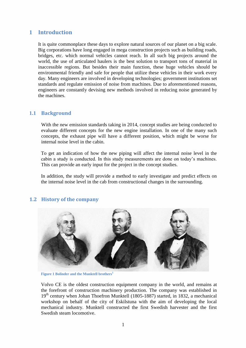
1.2 History of the company

Figure 1 Bolinder and the Munktell brothers1

Volvo CE is the oldest construction equipment company in the world, and remains at

the forefront of construction machinery production. The company was established in

19th

century when Johan Thoefron Munktell (1805-1887) started, in 1832, a mechanical

workshop on behalf of the city of Eskilstuna with the aim of developing the local

mechanical industry. Munktell constructed the first Swedish harvester and the first

Swedish steam locomotive.

2

In 1883, two brothers, Jean Bolinder (1813-1899) and Carl Gerhard Bolinder (1818-

1892) became famous thanks to the design of the first armed submarine. In the

following years they invented the first Swedish combustion engine and the steam roller.

In 1927 in Stockholm, Assar Gabrielsson and Gustaf Larsson established an automobile

company aiming at the public. It was the early keystone of Volvo CE.

In 1932, Sweden faced mounting economical problems, as a result of the Great

Depression in USA. Then the Handelsbanken bank decided to save assets within the

engineering industry. Consequently, companies of Munkel and Bolinder brothers were

merged into AB Bolinder-Munktell company.

After the Second World war, the future of AB Bolinder-Munktell was uncertain, as the

Handelsbanken bank wanted to break free the dependence of the industry. AB Bolinder-

Munktell recieved two offers, one was International Harvester from USA, while the

second one was Volvo, which successfully acquired Bolinder-Munktell in May of 1950.

In the late 1950s, in Braås, Livab was experimenting with machines to connect driven

hauler trailers and tractors. Development of the machine picked up speed in 1965, when

Bolinder-Mounktell signed agreement with Livab. One year later Volvo BM introduced

world’s first series manufactured articulated hauler DR 631.

Twenty years later Volvo merged with the American companies Clark and Euclid and

formed the VME-group, which established Volvo Construction Equipment in 1995.

Nowadays Volvo CE has about 35 per cent of the worldwide market. With the new F-

series of articulated hauler the company wants to win in the Asian market. 1

1.2.1 Articulated hauler Volvo A30F

The machine on which we carried out measurements is one out of four available

models; A30 F has 6-cylinder engine, which has 11 liters of capacity and 357

horsepower. Maximum load is 28 000 kg, and then articulated hauler weight is 51 200

kg.

Figure 2 Articulated Hauler Volvo A30F

3

1.3 Problem formulation

Moving the exhaust pipe to the shoulder cavity of the articulated hauler will affect the

sound pressure level in the cabin. We have to quantify the sound power level of the

exhaust pipe in the present machine and then place a sound source in the shoulder

cavity to determine the sound pressure level in the cabin. This will lead to the following

problem:

Determine the sound pressure level Lp2 in the cabin from the airborne sound from

vibration pipe at the new position 2, which is the shoulder cavity of the articulated

hauler.

1.4 Purpose

The purpose of this project is to quantify the sound source strength of the pipe and use a

reference sound source (RSS) with the same strength in the shoulder cavity of the

articulated hauler to determine the effect on the internal noise in the cabin.

1.5 Limitations/delimitations

We do not have access to a prototype. Therefore the measurements are done on the

present machine Volvo A30F which would give us an estimate.

The method we are using is not exact but it is better than calculation not based on

measurement result.

The assumptions and their limitations that are used in the method we use are the

following.

These assumptions and their limitations are:

1. The sound power level of the reference sound source (LwRSS) is not constant. It has

negligible effect and we can neglect it.

2. The reference sound source (RSS) and real sound source has not the same

directional radiation properties.

3. The real sound source has dimensions that are not small in comparison with the

distance to the cabin.

4. RSS will only give airborne sound where as the real sound source will also give

structure borne sound.

The errors associated with the first assumption can easily be neglected. Errors

associated with the 2nd

and 3rd

assumptions are important errors which will gives us

error of several dB.

Errors associated with the 4th

assumption are inherit in the method since the method

only takes airborne sound into account and not structure borne sound.

4

2 Research methodology

To estimate the sound level in the cabin by moving the exhaust pipe to a new location,

two methods can be employed.

The first method is to use sound intensity which is theoretically the best one but

practically it is complicated since the contribution from each component of the machine

has to be isolated. Therefore, we did not use this method.

The second method is to determine the sound power level of the exhaust pipe, calibrate

the sound source, and then place a sound source in the cavity to determine the sound

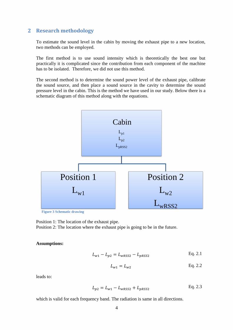
pressure level in the cabin. This is the method we have used in our study. Below there is a

schematic diagram of this method along with the equations.

Figure 3 Schematic drawing

Position 1: The location of the exhaust pipe.

Position 2: The location where the exhaust pipe is going to be in the future.

Assumptions:

leads to:

which is valid for each frequency band. The radiation is same in all directions.

CabinLp1

Lp2

LpRSS2

Position 1

Lw1

Position 2

Lw2

LwRSS2

Eq. 2.1

Eq. 2.2

Eq. 2.3

5

Here:

- - sound power level of the exhaust pipe

- - sound pressure level in the cabin (this is what we have to find)

- - sound power level of the reference sound source

- - sound pressure level in the cabin due to the sound source in the cavity

Below we explain how , , are determined.

The sound power level of the exhaust pipe is determined by mounting accelerometers

on the exhaust pipe and using the equation below. The equation is valid for each

frequency band:

[dB]

Here:

- – vibration velocity level (dB)

- – surface of the pipe

- – correction factor

- - radiation efficiency of the pipe

- logarithm base is 10

The correction factor and the radiation efficiency of the pipe are given in

appendices 3-5.

The accelerometers measured the velocity of the vibrating exhaust pipe in the normal

direction to the surface only since the exhaust pipe doesn’t radiate sound in other

directions. We measured it using the 1/3 octave band. The velocity data we obtained from

the measurements were used in the equation for each frequency band, and the logarithmic

mean value of the sound power level was calculated.

is determined by calibrating the sound source outdoors at the Volvo CE sound

testing facility in Braås and using the equation below, which is valid for each frequency

band:

[dB]

Here:

- – sound pressure level (dB)

- – surface of the measurement half sphere (radius is 2 meters)

- – sound power level of the sound source (speaker)

The calibrated sound power level of the sound source as function of feeding

voltage, valid for each frequency band, is:

[dB]

Here:

- – the voltage at which the sound pressure level is calibrated.

- – the voltage at which the sound pressure level in the cabin is measured.

Eq. 2.4

Eq. 2.5

Eq. 2.6

6

- – calibrated sound power level of the sound source.

- – sound pressure level in the cabin

Both and are 1/3 octave band values that are functions of frequency.

is determined by placing two microphones inside the cabin which measure the

sound pressure level due to the sound power level of the sound source in the shoulder

cavity of the articulated hauler when the engine is turned off.

The equation we use to calculate the logarithmic mean value for each frequency band is:

[dB]

Here:

- - sound pressure level of the left microphone

- - sound pressure level of the right microphone

Eq. 2.7

7

3 Theory

In this chapter basic definition are explained. Description of measurement components

you can find in appendix 2.

3.1 Sound, frequency

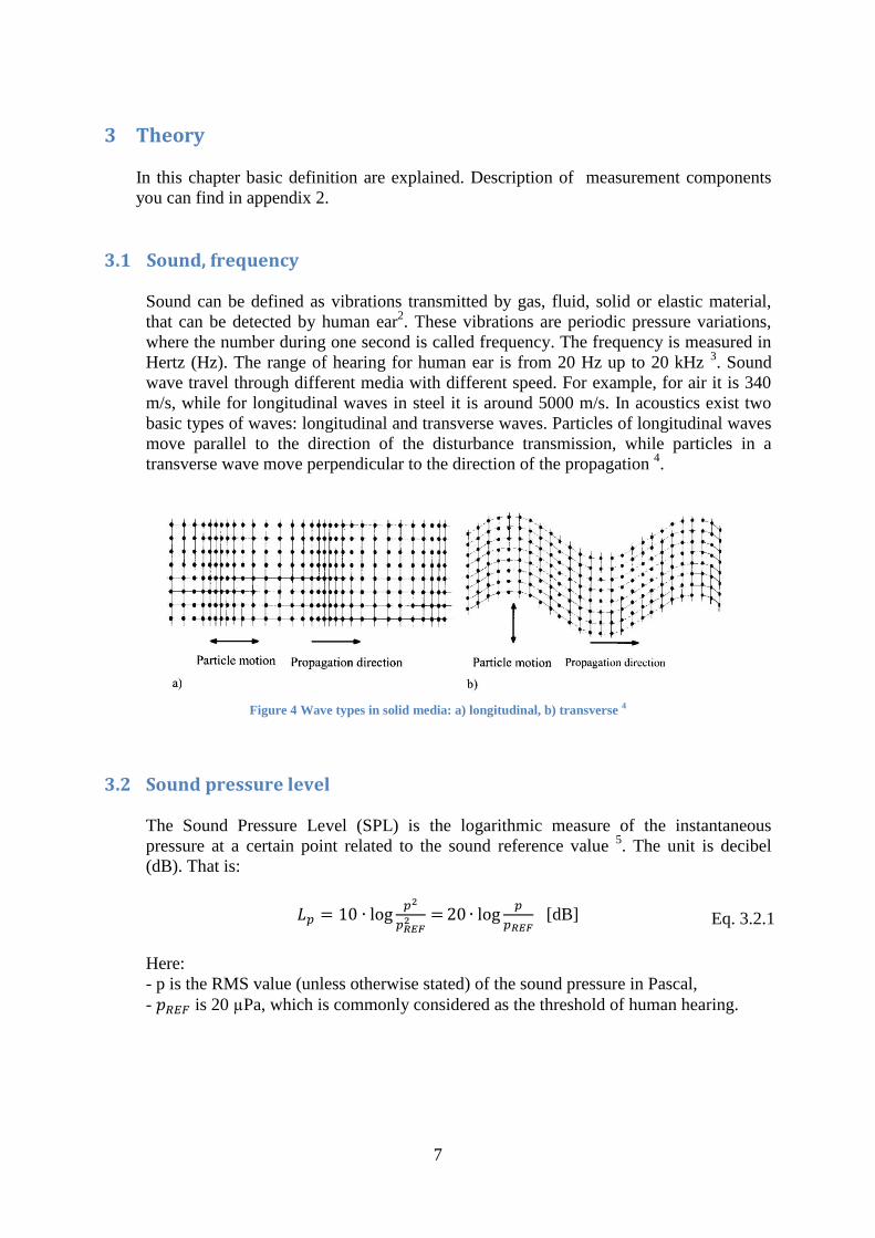
Sound can be defined as vibrations transmitted by gas, fluid, solid or elastic material,

that can be detected by human ear2. These vibrations are periodic pressure variations,

where the number during one second is called frequency. The frequency is measured in

Hertz (Hz). The range of hearing for human ear is from 20 Hz up to 20 kHz 3. Sound

wave travel through different media with different speed. For example, for air it is 340

m/s, while for longitudinal waves in steel it is around 5000 m/s. In acoustics exist two

basic types of waves: longitudinal and transverse waves. Particles of longitudinal waves

move parallel to the direction of the disturbance transmission, while particles in a

transverse wave move perpendicular to the direction of the propagation 4.

Figure 4 Wave types in solid media: a) longitudinal, b) transverse 4

3.2 Sound pressure level

The Sound Pressure Level (SPL) is the logarithmic measure of the instantaneous

pressure at a certain point related to the sound reference value 5. The unit is decibel

(dB). That is:

[dB]

Here:

- p is the RMS value (unless otherwise stated) of the sound pressure in Pascal,

- is 20 µPa, which is commonly considered as the threshold of human hearing.

Eq. 3.2.1

8

3.3 Sound power level

The Sound Power Level is defined as the logarithmic measure of the absolute value of

the sound power generated by a source related to the specified sound power reference

level 6. The unit is watt (W). That is:

[dB]

Here:

- is the value of sound power of the source,

- is 10-12

W.

3.4 Weighting filters

Weighting filters are commonly used in acoustics to amplify differently the signal of the

microphone in different frequency ranges. Human hearing adjusts to both frequency and

strength of the sound 4. The human ear is most sensitive in the medium range of audible

frequencies, while in very low and very high ones it is insensitive. Weighting filters

emphasize or attenuate frequencies and in case of human perception of sound, A-filter is

the most common one.

Figure 5 A, B, C, D-weighting curves 4

Eq. 3.3.1

9

4 Measurement setup

Schematic diagrams of each measurement setup are given in appendix 1.

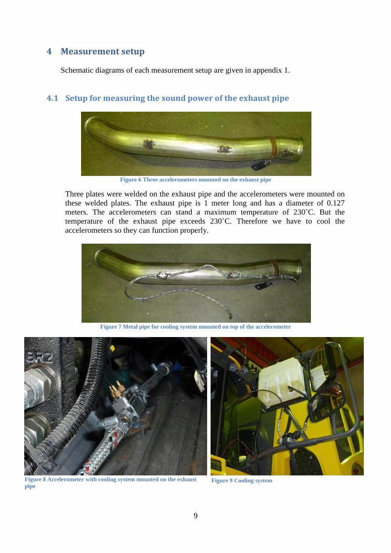
4.1 Setup for measuring the sound power of the exhaust pipe

Figure 6 Three accelerometers mounted on the exhaust pipe

Three plates were welded on the exhaust pipe and the accelerometers were mounted on

these welded plates. The exhaust pipe is 1 meter long and has a diameter of 0.127

meters. The accelerometers can stand a maximum temperature of 230˚C. But the

temperature of the exhaust pipe exceeds 230˚C. Therefore we have to cool the

accelerometers so they can function properly.

Figure 7 Metal pipe for cooling system mounted on top of the accelerometer

Figure 9 Cooling system Figure 8 Accelerometer with cooling system mounted on the exhaust

pipe

10

Figure 10 LMS SCADAS Mobile Front-end during measurements

The accelerometer has 3 directions x,y,z and are attached to the channels in the

front-end measuring system. The front end is attached to the PC and using LMS

software the data obtained from the measurements.

11

4.2 Setup for calibrating the sound source

Figure 11 Setup for calibrating sound source - on the picture sound source and two microphones

This is the sound testing facility at VOLVO CE. Two microphones placed in the half of

a sphere to measure the sound pressure level. The ground is hard, reflecting and there

are no reflections from buildings etc.

Figure 12 Setup for calibrating sound source – on the picture amplifier, front-end and splitter

LMS Front-end and Amplifier. The sound source is connected to the amplifier and the

LMS front End is connected to the PC. The splitter divides the voltage of the sound

source since the front-end can only take 12 V.

12

4.3 Setup for measuring the sound pressure level inside the cabin

Figure 13 The Cavity where we put the sound source

The cavity where we put the sound source(speaker). A wave file was generated from the

accelerometers measurement. We used it as a signal generator to simulate the sound

from the exhaust pipe. The microphones measured the sound pressure level in the cabin

while the engine was turned off and the only source of sound was through the speaker.

Figure 14 The sound source is mounted inside the cavity

13

Figure 15 Setup for measuring the sound pressure level inside the cabin

Figure 16 Two Microphones mounted on a stand to measure

the sound pressure level inside the cabin

Two Microphones mounted on a stand to measure the sound pressure level inside the

cabin when we played the exhaust pipe sound in the speaker.

14

5 Results

Here, we present the final result of our calculations in total levels in dBA. We did all the

measurements and calculations using 1/3 octave bands. Results in 1/3 octave bands are

shown in appendix 8. However, these results don’t take frequencies below 80 Hz,

including the first harmonic and the fundamental frequency, into account.

The sound power level Lw1 of the exhaust pipe is determined by Equation 2.4 and the

sound pressure level Lp2 in the cabin is determined by Equation 2.3, that is rewritten as:

We use the reference sound source to determine , and the result is

presented in the figure 3 in appendix 8.

It is worth to mention here that the sound source was wrapped in plastic as shown in

figure 14. We assume that it has negligible effect on the reference sound pressure level

LpRSS2.

The results presented below are for 3 cases. in all cases we have Lw1=Lv+10logS+C+Re,

where C=146,1 dB. For the three cases we have the following:

Case 1: Re=0

Case 2: Re for n=0 (monopole)

Case 3: Re for n=1 (dipole)

For details on Re, see appendices 4 and 5.

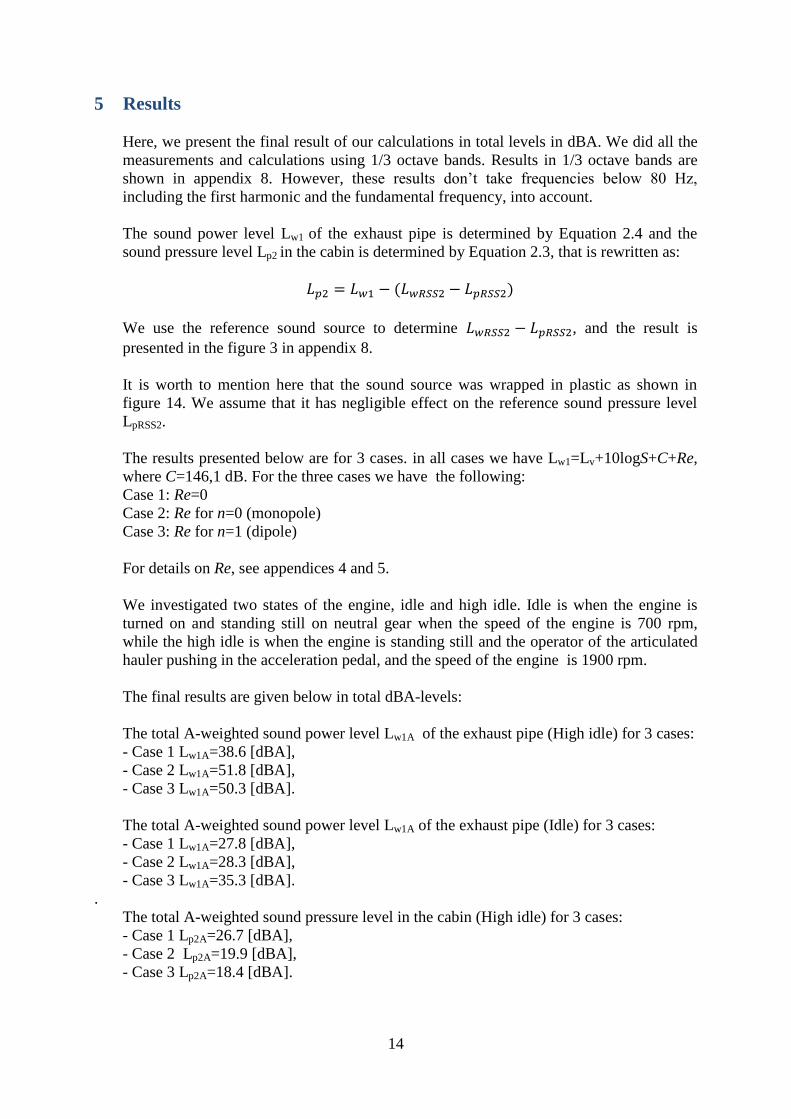
We investigated two states of the engine, idle and high idle. Idle is when the engine is

turned on and standing still on neutral gear when the speed of the engine is 700 rpm,

while the high idle is when the engine is standing still and the operator of the articulated

hauler pushing in the acceleration pedal, and the speed of the engine is 1900 rpm.

The final results are given below in total dBA-levels:

The total A-weighted sound power level Lw1A of the exhaust pipe (High idle) for 3 cases:

- Case 1 Lw1A=38.6 [dBA],


- Case 3 Lw1A=50.3 [dBA].

The total A-weighted sound power level Lw1A of the exhaust pipe (Idle) for 3 cases:



- Case 3 Lw1A=35.3 [dBA].

.

The total A-weighted sound pressure level in the cabin (High idle) for 3 cases:

- Case 1 Lp2A=26.7 [dBA],


- Case 3 Lp2A=18.4 [dBA].

15

The total A-weighted sound pressure level in the cabin (Idle) for 3 cases:



- Case 3 Lp2A=1.1 [dBA].

Figure 17 Difference between cases

Figure 17 shows the radiation Re of the exhaust pipe as function of frequency. At any

given frequency we can find the corresponding radiation efficiency of the exhaust pipe.

Note that Lw1,case2-Lw1,case1=Re for n=0 and Lw1,case3-Lw1,case1=Re for n=1.

On the next page we present the final results in 1/3 octave band.

-60,0

-50,0

-40,0

-30,0

-20,0

-10,0

0,0

10,0

20,0

30,0

80

10

0

12

5

16

0

20

0

25

0

31

5

40

0

50

0

63

0

80

0

10

00

12

50

16

00

20

00

25

00

31

50

40

00

50

00

Rad

iati

on

eff

icie

ncy

Re

Frequency f

Lw1,case 2-Lw1,case 1 monopole (n=0)

Lw1,case 3-Lw1,case 1 dipole (n=1)

16

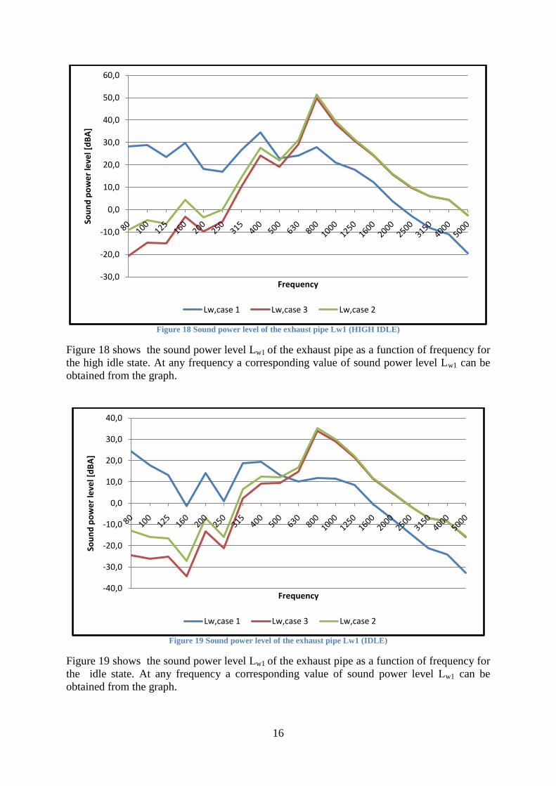
Figure 18 Sound power level of the exhaust pipe Lw1 (HIGH IDLE)

Figure 18 shows the sound power level Lw1 of the exhaust pipe as a function of frequency for

the high idle state. At any frequency a corresponding value of sound power level Lw1 can be

obtained from the graph.

Figure 19 Sound power level of the exhaust pipe Lw1 (IDLE)

Figure 19 shows the sound power level Lw1 of the exhaust pipe as a function of frequency for

the idle state. At any frequency a corresponding value of sound power level Lw1 can be

obtained from the graph.

-30,0

-20,0

-10,0

0,0

10,0

20,0

30,0

40,0

50,0

60,0So

un

d p

ow

er

leve

l [d

BA

]

Frequency

Lw,case 1 Lw,case 3 Lw,case 2

-40,0

-30,0

-20,0

-10,0

0,0

10,0

20,0

30,0

40,0

Sou

nd

po

we

r le

vel [

dB

A]

Frequency

Lw,case 1 Lw,case 3 Lw,case 2

17

Figure 20 Sound pressure level Lp2 in the cabin (high idle)

Figure 20 shows the sound pressure level Lp2 as a function of frequency for the high idle state.

At any frequency a corresponding value of sound pressure level Lp2 can be obtained from the

graph.

Figure 21 Sound pressure level Lp2 in the cabin (idle)

Figure 21 shows the sound pressure level Lp2 as a function of frequency for the idle state. At

any frequency a corresponding value of sound pressure level Lp2 can be obtained from the

graph.

-80,0

-60,0

-40,0

-20,0

0,0

20,0

40,0

Sou

nd

pre

ssu

re le

vel [

dB

A]

Frequency

Lp2,case1 Lp2,case3 Lp2,case2

-100,0

-80,0

-60,0

-40,0

-20,0

0,0

20,0

40,0

Sou

nd

pre

ssu

re le

vel [

dB

A]

Frequency

Lp2,case1 Lp2,case3 Lp2,case2

18

6 Analysis and discussion

Here, we analyze the results presented in the previous section. First we analyze the radiation

efficiency Re of the pipe for different cases (Fig.17), then the sound power level Lw1 (Fig. 18,

19) of the exhaust pipe, finally we discuss result for the main purpose of interest, namely the

sound pressure level Lp2 in the cabin (Fig. 20, 21) are given below.

Figure 17 shows that at low frequencies there is a large difference between the radiation

efficiency for the 2 cases whereas at high frequencies above 800 Hz, the radiation efficiency

for both cases are identical . At 800 Hz the radiation efficiency for both cases is peaking there.

Figure 18 shows that at low frequencies the sound power level of the exhaust pipe for each

case is not dominating. For case 2 and 3, the sound power level is at its peak around 800 Hz.

The reason for this is that the radiation efficiency is peaking there.

For frequencies above 2000 Hz the sound power level of the exhaust pipe is of minor

importance for all three cases due to the spectrum of the sound source. For frequencies below

300 Hz the sound power level is of minor importance for case 2 and 3 due to reduced

radiation efficiency.

Figure 19 shows that at low frequencies the sound power level of the exhaust pipe for each

case is not dominating. For case 2 and 3, the sound power level is at its peak around 800 Hz

the reason for this is that the radiation efficiency is peaking there.

For frequencies above 2000 Hz the sound power level of the exhaust pipe is of minor

importance for all three cases due to the spectrum of the sound source. For frequencies below

300 Hz the sound power level is of minor importance for case 2 and 3 due to reduced

radiation efficiency

Finally we discuss the sound pressure level in the cabin.

Figure 20 shows that at 80 Hz the sound pressure level for case 1 has its maximum value

within the presented frequency range, but for other 2 cases it’s insignificant at this frequency.

Around 800 Hz the sound pressure level for case 2 and 3 is peaking there.

For frequencies above 1250 Hz the sound pressure level for all three cases is of minor

importance.

Figure 21 shows that at 80 Hz the sound pressure level for case 1 has its maximum value

within the presented frequency range, but for other 2 cases it is insignificant at this frequency.

Around 800 Hz the sound pressure level for case 2 and 3 is peaking there. For frequencies

above 125 Hz the sound pressure level for case 1 is of minor importance.

For frequencies above 80 Hz and 1000 Hz the sound pressure level for case 2 and 3 is

insignificant.

The highest sound level in the cabin is 26,7 dBA for high idle assuming that radiation

efficiency Re = 0 (case 1). This is much lower than the sound level during the operation,

which is 74 dBA. It is worth commenting that the total highest sound power level is not

always producing the highest sound level in the cabin. The main reason is that the frequency

dependence of the radiation efficiency is different for the three cases.

19

7 Conclusion

Based on the assumption that the accelerometers were properly calibrated, the movement

of the exhaust pipe to the new location does not affect the sound level in the cabin. The

sound pressure level for the both states, idle and high idle, is below 30 dBA while the

reference sound pressure level measured by Volvo CE in the cabin is 74 dBA. The

difference between these levels is over 40 dBA. Such a big difference does not increase

the sound pressure level in the cabin.

The results we obtained from the calculations do not take the fundamental, the first

harmonic of the firing frequency that are in 1/3 octave frequency bands below 80 Hz.

8 Recommendations

It is recommended to check the calibration of the accelerometers after dismounting them.

The difference in sensitivity of the accelerometers between measured and factory data

can be used to correct the results in this report.

In the current case the calculated sound level in the cabin from the pipe at its in new

location was much lower than the sound level during operation. So despite that the

accuracy of the method is rather poor it is possible to draw the conclusion that sound

level in the cabin will not be affected by the movement of the pipe. if, however the

calculated had been closer to the operating sound level a more accurate method had to be

used. The most critical part is the radiation efficiency Re that on this case require the

more precise determination.

It is also worth mentioning that correlation measurements could sometimes be of value.8

20

9 References

Books:

4. Wallin, H.P. and Carlsson, U. and Åbom, M. and Bodén, H. and Glav, R. (2010).

Sound and Vibration. Kungl Tekniska Högskolan

Internet:

1. Volvo CE. (2007). 175 years Volvo Construction Equipment 1832 - 2007.

Http://www.volvo.com/NR/rdonlyres/39862192-0CD5-4770-9D50-

1ECAEA20377B/0/175years21A10039610711.pdf (accessed 20 may, 2011, time 11.50)

2. Sound, http://dictionary.reference.com/browse/sound (accessed 20 may, 2011, time

12.55)

3. Brüel & Kjær, (1984). Measuring the sound.

http://www.bksv.com/Library/Primers.aspx (accessed 6 may, 2011, time 19.30)

5. Brüel & Kjær, (1996) Microphone handbook vol. 1.


6. LMS Theory Tutorial.

http://www.lmsintl.com/downloads/tutorials (accessed 2 may, 2011, time 11.00)

7. Brüel & Kjær, (1982) Measuring Vibration.


8. Ovcina, A. and Petersson, M. (2005) Ljud- och vibrationsnivåer i en dumper

mätningar och analys.

http://w3.msi.vxu.se/~bni/akustik-volvo2.pdf (accessed 9 may, 2011, time 16.47)

http://www.bksv.com/AboutUs/AboutBruelAndKjaer.aspx



21

10 Appendix

Appendix 1 Schematic drawings of measuring position 2

Appendix 2 Measurement system components 6

Appendix 3 Derivation of the correction factor 1

Appendix 4 Calculation of the sound power level of the exhaust pipe 1

Appendix 5 Acoustic radiation form acoustic cylindrical multipoles 2

Appendix 6 Calculation of cabin reference sound pressure 1

Appendix 7 Calculation of calibration of the sound source 1

Appendix 8 Measurement data and calculations. 2

Appendix 9 Example of calculations. 2

Appendix 10 Summary and analysis of measurements on a VOLVO Articulated Hauler 6

1 of 2

Appendix 1 Schematic drawings of measuring position

Sound Power Level measuring position schematic diagram.

Sound Pressure Level measuring position schematic diagram

COOLING

SYSTEM

FRONT-END

COMPUTER

A A A

EXHAUST PIPE

ACCELEROMETER

CABIN

MICROPHONE

M M

COMPUTER

FRONT-END

SPLITTER

SOUND

SOURCE

AMPLIFIER

2 of 2

Calibration of the sound source schematic diagram.

SOUND

SOURCE M

M

FRONT-END

AMPLIFIER

SPLITTER

COMPUTER

MICROPHONE

1 of 6

Appendix 2

Measurement system components

Accelerometer

Accelerometers can measure the acceleration in different directions. The triaxial

piezoelectric charge accelerometer Brüel & Kjær type 4326-A-001 can stand high

temperatures in comparison to other available ones. A mechanical stress generates

proportional electrical charge to the force, which was applied to accelerometer 7.

Figure 1 Accelerometer type 4326-A-001

THE TRIAXIAL PIEZOELECTRIC CHARGE ACCELEROMETER

BRÜEL & KJÆR TYPE 4326-A-001

Frequency 1 - 8000 Hz

Temperature -55 - 230 ºC (-67.0 -

446.0 °F)

Weight 17 gram

Sensitivity 3 pC/g

Residual Noise Level in Spec Freq Range (rms) ± 0.30 mg

Maximum Operational Level (peak) 2000 g

Electrical Connector 10-32 UNF

Mounting Adhesive

Accessory Included None

Clip/Stud/Screw included None

Output Charge-PE

Unigain No

Triaxial Yes

TEDS No

Resonance Frequency 30 kHz

Maximum Shock Level (± peak) 5000 g

table 1 the triaxial piezoelectric charge accelerometer Brüel & Kjær type 4326-A-001

2 of 6

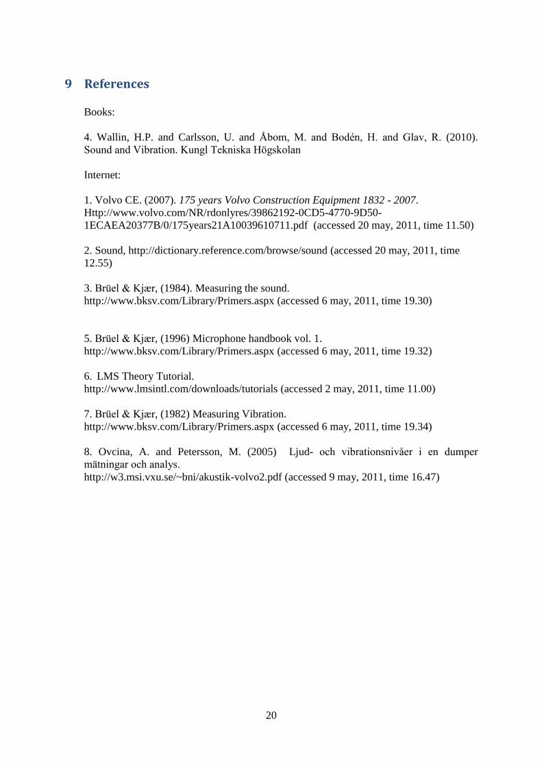
Front-end

LMS SCADAS Mobile SCM05, produced by LMS Engineering Innovation, is the high-

end measurement system, which perfectly suits to advanced engineering noise and

vibration testing. The system consists of 40 input channels, CAN bus system, Bluetooth

as well as GPS.

Figure 2 LMS SCADAS Mobile SCM05

Table 2 LMS SCADAS Mobile SCM05

LMS SCADAS Mobile SCM05

Number of slots 6 (1 for system controller)

Max number of channels per frame 40

Tacho inputs 2 (standard on board)

Generator outputs 2 (standard on board)

Dimensions (WxHxD) 340 x 78 x 295 mm

13.38 x 3.07 x 11.69 inch

Weight 6.2kg max / 13.67 lbs max

AC power input 110/220V

DC power input 9-36V

Max power consumption 40W

Battery operation (minimum) 1 hour (4 hours with additional slot battery)

Host interface Ethernet

Operating temperature -10°C to +55°C / 14° to 131°F

Sensor type V, ICP, MIC, charge, strain, digital audio

3 of 6

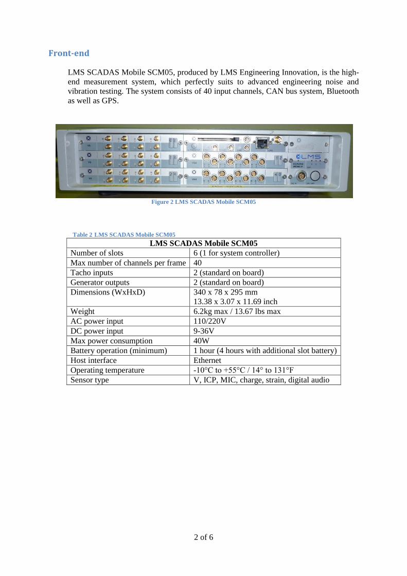
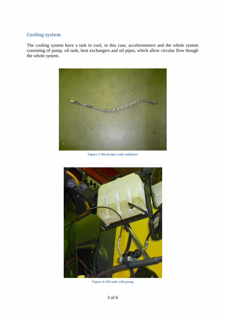
Cooling system

The cooling system have a task to cool, in this case, accelerometers and the whole system

consisting of pump, oil tank, heat exchangers and oil pipes, which allow circular flow though

the whole system.

Figure 3 Metal pipe with radiators

Figure 4 Oil tank with pump

4 of 6

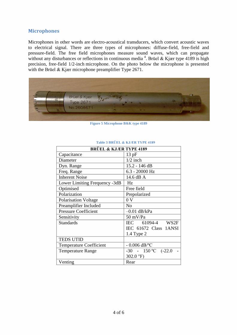
Microphones

Microphones in other words are electro-acoustical transducers, which convert acoustic waves

to electrical signal. There are three types of microphones: diffuse-field, free-field and

pressure-field. The free field microphones measure sound waves, which can propagate

without any disturbances or reflections in continuous media 4. Brüel & Kjær type 4189 is high

precision, free-field 1/2-inch microphone. On the photo below the microphone is presented

with the Brüel & Kjær microphone preamplifier Type 2671.

Figure 5 Microphone B&K type 4189

Table 3 BRÜEL & KJÆR TYPE 4189

BRÜEL & KJÆR TYPE 4189

Capacitance 13 pF

Diameter 1/2 inch

Dyn. Range 15.2 - 146 dB

Freq. Range 6.3 - 20000 Hz

Inherent Noise 14.6 dB A

Lower Limiting Frequency -3dB Hz

Optimised Free field

Polarization Prepolarized

Polarisation Voltage 0 V

Preamplifier Included No

Pressure Coefficient –0.01 dB/kPa

Sensitivity 50 mV/Pa

Standards IEC 61094-4 WS2F

IEC 61672 Class 1ANSI

1.4 Type 2

TEDS UTID

Temperature Coefficient - 0.006 dB/ºC

Temperature Range -30 - 150 ºC (-22.0 -

302.0 °F)

Venting Rear

5 of 6

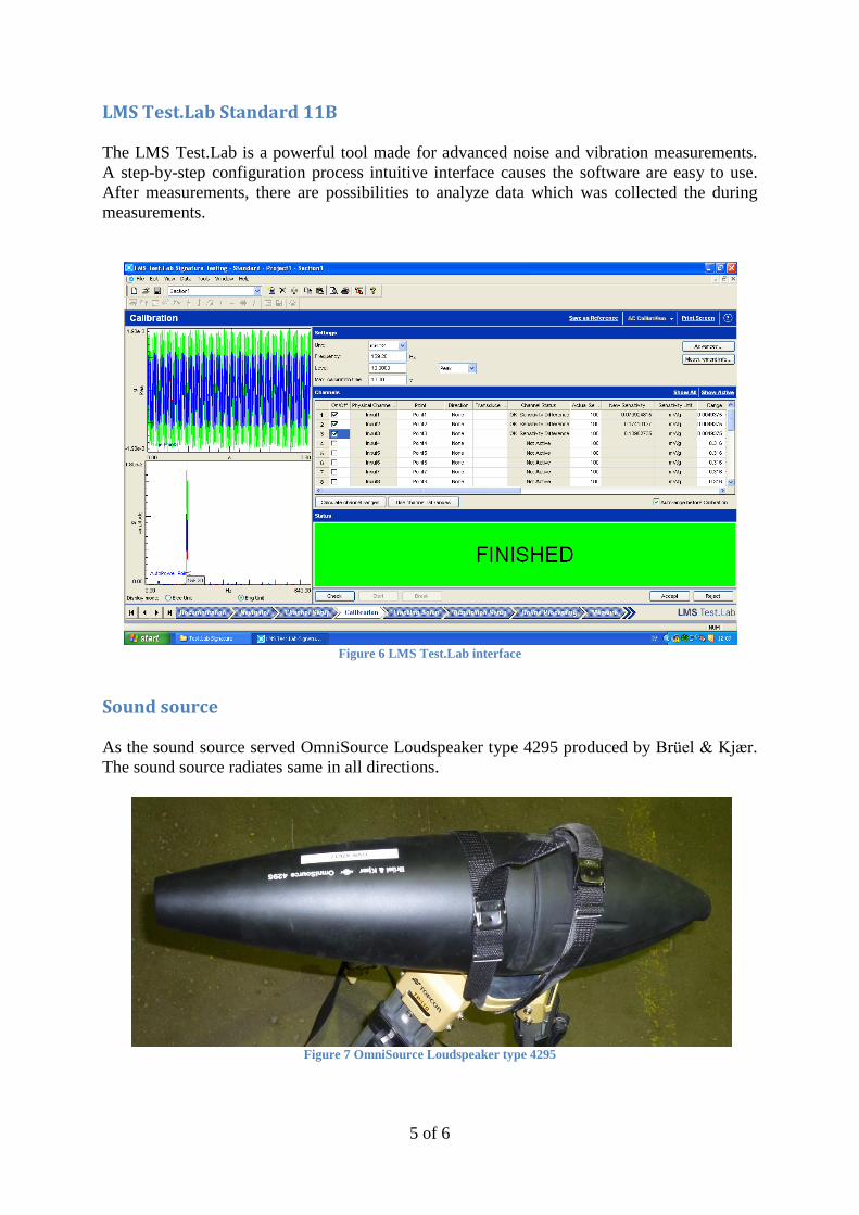
LMS Test.Lab Standard 11B

The LMS Test.Lab is a powerful tool made for advanced noise and vibration measurements.

A step-by-step configuration process intuitive interface causes the software are easy to use.

After measurements, there are possibilities to analyze data which was collected the during

measurements.

Figure 6 LMS Test.Lab interface

Sound source

As the sound source served OmniSource Loudspeaker type 4295 produced by Brüel & Kjær.

The sound source radiates same in all directions.

Figure 7 OmniSource Loudspeaker type 4295

6 of 6

Splitter

With the help of a splitter, it is possible to adjust the voltage of the amplifier to the front-end.

The splitter divides the voltage in the ratio of 1:4. The splitter has 4 input and 4 output

sockets.

Figure 8 Splitter

1 of 1

Appendix 3 Derivation of the correction factor

We assume first a plane wave and therefore we can use

eq.12.1

eq.12.2

We need to find a relationship between the velocity and the sound power. Therefore we

isolate p (eq.1.2) and inserting this expression into eq.1.1 .We get the formula below (eq.1.3).

eq.12.3

eq.12.4

Inserting eq.1.3 into above we get equation 1.5 and we introduce so we can get an

expression for Lv

eq.12.5

Following the logarithmic rules for multiplication we get eq 1.6

eq.12.6

Where the first term in the eq.1.6 is a velocity level and the last term in the eq.1.6 is a

correction factor.

eq.12.7

Nomenclature:

– Power,

– velocity,

– speed of sound in the air, app. 340m/s

- density of air, app. 1,2 kg/m3

- Sound power level

– Surface of the area

– pressure

– reference value of the velocity

- vibration velocity level

– correction factor

- power reference value

Log - base 10

Next we assume a more complicated radiation pattern, please see appendix 5 for a derivation.

1 of 1

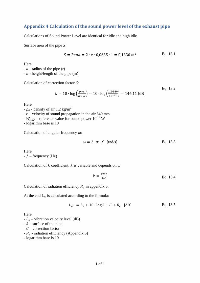
Appendix 4 Calculation of the sound power level of the exhaust pipe

Calculations of Sound Power Level are identical for idle and high idle.

Surface area of the pipe :

Here:

- - radius of the pipe (r)

- - height/length of the pipe (m)

Calculation of correction factor :

[dB]

Here:

- - density of air 1,2 kg/m3

- c – velocity of sound propagation in the air 340 m/s

- – reference value for sound power 10-12

W


Calculation of angular frequency :

[rad/s]

Here:

- – frequency (Hz)

Calculation of coefficient. is variable and depends on .

Calculation of radiation efficiency in appendix 5.

At the end Lw is calculated according to the formula:

[dB]

Here:

- – vibration velocity level (dB)

- – surface of the pipe

- – correction factor

- - radiation efficiency (Appendix 5)


Eq. 13.1

Eq. 13.2

Eq. 13.3

Eq. 13.4

Eq. 13.5

1 of 2

Appendix 5 Acoustic radiation form acoustic cylindrical multipoles

2 of 2

1 of 1

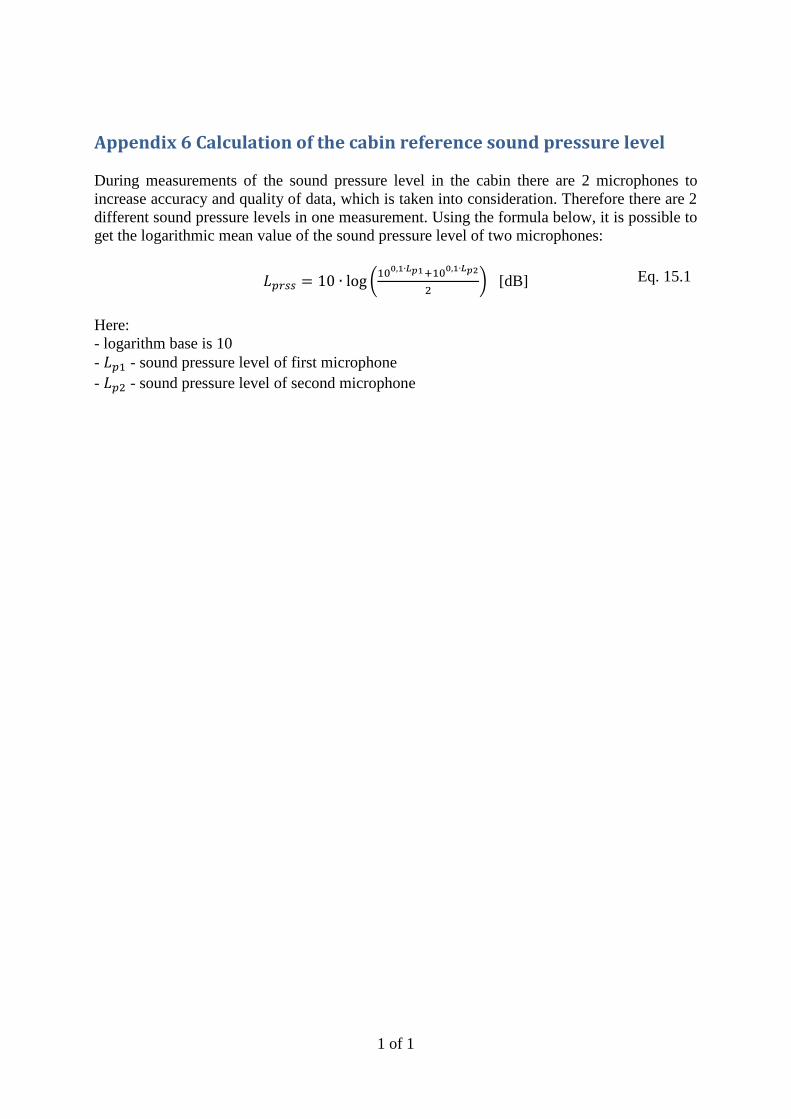
Appendix 6 Calculation of the cabin reference sound pressure level

During measurements of the sound pressure level in the cabin there are 2 microphones to

increase accuracy and quality of data, which is taken into consideration. Therefore there are 2

different sound pressure levels in one measurement. Using the formula below, it is possible to

get the logarithmic mean value of the sound pressure level of two microphones:

[dB]

Here:


- - sound pressure level of first microphone

- - sound pressure level of second microphone

Eq. 15.1

1 of 1

Appendix 7 Calculation of calibration of the sound source

Calculation of the sphere area S:

[m2]

Here:

- - radius of the sphere

Calculation of logarithmic mean value of sound pressure levels of microphones :

[dB]

Here:


- - sound pressure level of first microphone

- - sound pressure level of second microphone

Calculation of Sound Power Level of sound source :

[dB]

Here:

- S – surface area of half sphere

- – logarithmic mean value of sound pressure levels of microphones, which were used

during calibration.


Calculation of the calibrated Sound Power Level

[dB]

Here:


- - Sound Power Level of the sound source

- – voltage of Sound Pressure Level of calibration

- - voltage of Sound Pressure Level in the cabin

- – calibrated Sound Power Level of sound source

Eq. 16.1

Eq. 16.2

Eq. 16.3

Eq. 16.4

1 of 2

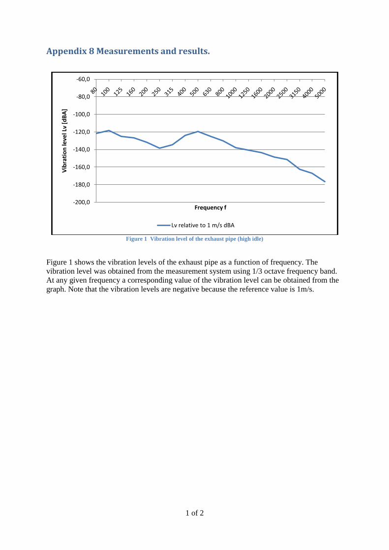
Appendix 8 Measurements and results.

Figure 1 Vibration level of the exhaust pipe (high idle)

Figure 1 shows the vibration levels of the exhaust pipe as a function of frequency. The

vibration level was obtained from the measurement system using 1/3 octave frequency band.

At any given frequency a corresponding value of the vibration level can be obtained from the

graph. Note that the vibration levels are negative because the reference value is 1m/s.

-200,0

-180,0

-160,0

-140,0

-120,0

-100,0

-80,0

-60,0

Vib

rati

on

leve

l Lv

[dB

A]

Frequency f

Lv relative to 1 m/s dBA

2 of 2

Figure 2 Vibration level of the exhaust pipe (idle)

Figure 2 shows the vibration levels of the exhaust pipe as a function of the frequency. The

vibration level was obtained from the measurement system using 1/3 octave frequency band.

At any given frequency a corresponding value of the vibration level can be obtained from the

graph. Note that the vibration levels are negative because the reference value is 1m/s.

Figure 3 LwRSS2-LpRSS2

Figure 3 shows the difference between LwRSS2-LpRSS2 as a function of frequency and the

voltage as a function of frequency. At any frequency we can determine the corresponding

voltage and the difference between LwRSS2-LpRSS2. At 6300 Hz the difference between LwRSS2-

LpRSS2 is maximum within this frequency range. Note that LwRss2-LprSS is average value of

the two states because the LwRSS2-LpRSS2 we obtained for two states were different.

-200,0

-180,0

-160,0

-140,0

-120,0

-100,0

-80,0

-60,0

Vib

rati

on

leve

l [d

BA

]

Frequency f

Lv relative to 1m/s dBA

-80,0

-60,0

-40,0

-20,0

0,0

20,0

40,0

60,0

80

10

0

12

5

16

0

20

0

25

0

31

5

40

0

50

0

63

0

80

0

10

00

12

50

16

00

20

00

25

00

31

50

40

00

50

00

63

00

80

00

10

00

0

12

50

0

16

00

0

dB

A

Frequency f

LwRSS2-LpRSS2 Voltage

1 of 2

Appendix 9 Example of calculations

We are going to show how we obtained the sound pressure level in the cabin from the

equation 2.3.

All calculations were done for high idle state, case 1 and for frequency of 800 Hz. Case 1 take

only correction factor into consideration. All logarithms base is 10.

To calculate we used equation 2.4, that is given below:

From the equation above we have given from measurement and it is equal to -129.2 dB.

Now we have to calculate second component, which is . We assumed that length of

the pipe is cylindrical, straight, 1m long and diameter is 5 in, which is 0.127m. Hence:

Because result is negative, we put result in absolute value.

To calculate correction factor we used equation, where is density of air 1,2 kg/m3, c is

velocity of sound propagation in the air 340 m/s, and is reference value for sound power

10-12

W. Having all necessary data we can do following calculation:

[dB]

Due to the fact that our calculation were made for case 1, radiation efficiency is equal to 0.

Then equation 2.4 looks:

So now we calculated first component of equation 2.3. Now we can calculate second

component, which is calibrated sound power level of the reference sound source using

equation 2.6, which you can see below:

[dB]

is the mean value (Eq.2.7) of the microphones in the cabin, which is equal to 50,4 dB.

In the equation 2.6 we have to calculate surface S of the halfsphere (radius is 2m), which is

equal to 25,14 m2. is the voltage at which the sound pressure level is calibrated and is

equal to 0,67V. is the voltage at which the sound pressure level in the cabin is measured

and is equal to 0,94. Having all components from equation 2.6 we can calculate value of

:

2 of 2

Now we calculated value of second component of equation 2.3. The last component, which is

sound pressure level of the reference sound source. was used to calculate

in equation above. To get more detailed way of calculating you can find in

appendix 6.

Having all necessary components of equation 2.3 we can calculate sound pressure level in

cabin in position 2, hence:

When we calculate values of for every frequency in our measurement, we can calculate

total sound pressure level in the cabin in position 2, using the formula for mean value of

logarithm.

1 of 6

Appendix 10 Summary and analysis of measurements on a VOLVO Articulated Hauler

This document summarizes and analyses differences between three different evaluation

models. More details are found in the full report.

Measurement method The main goal of the investigation was to determine the sound level in the cabin from air

borne sound from a vibrating exhaust piping. The investigation was made in two parts.

A. Determination of the difference Lw-Lp between the sound power level Lw and sound

pressure level Lp for a reference sound source located at the same place as the exhaust

piping. Here, Lw was determined under three field conditions. The analysis was done

in 1/3 octave bands.

B. Determination of Lw for the exhaust piping using measurements of the velocity level

Lv on the surface of the exhaust piping.

The model was used to compute Lw-Lp in part A:

1) Lw-Lp=LwRSS2+LpRSS2

Three models were used to determine Lw-Lv in part B:

1) The far field assumption of a plane wave

Lw-Lv=10∙log S + C

2) Cylindrical monopole

Lw-Lv=10∙log S + C+Re|n=0

3) Cylindrical dipole

Lw-Lv=10∙log S + C+Re|n=1

Here, C is a frequency independent correction factor that describes the relation between

velocity level Lv and pressure level Lp in a plane wave. Re is the radiation efficiency.

Case 1, which has the advantage of being frequency independent, describes the physical

conditions poorly, can give an estimate only. Cases 2 and 3 should be able to describe the

situation better but with the complication that Re is frequency dependent. There is no

assumption about a plane far field for cases 2 and 3; in actual fact Re describes a transfer from

a cylindrical near field (below ca 600 Hz) via a resonant region at about 800 Hz to the

cylindrical far field (above ca 1000 Hz). Please c.f. Fig. 1 for a frequency plot of Re.

The analysis is performed in 1/3 octave bands to capture the frequency behaviour.

2 of 6

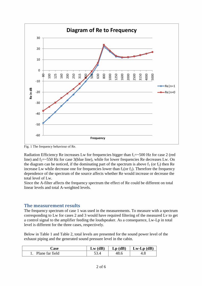
Fig. 1 The frequency behaviour of Re.

Radiation Efficiency Re increases Lw for frequencies bigger than f1=~500 Hz for case 2 (red

line) and f2=~550 Hz for case 3(blue line), while for lower frequencies Re decreases Lw. On

the diagram can be noticed, if the dominating part of the spectrum is above f1 (or f2) then Re

increase Lw while decrease one for frequencies lower than f1(or f2). Therefore the frequency

dependence of the spectrum of the source affects whether Re would increase or decrease the

total level of Lw.

Since the A-filter affects the frequency spectrum the effect of Re could be different on total

linear levels and total A-weighted levels.

The measurement results The frequency spectrum of case 1 was used in the measurements. To measure with a spectrum

corresponding to Lw for cases 2 and 3 would have required filtering of the measured Lv to get

a control signal to the amplifier feeding the loudspeaker. As a consequence, Lw-Lp in total

level is different for the three cases, respectively.

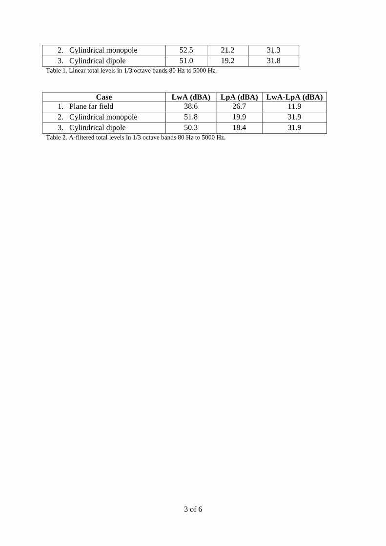
Below in Table 1 and Table 2, total levels are presented for the sound power level of the

exhaust piping and the generated sound pressure level in the cabin.

Case Lw (dB) Lp (dB) Lw-Lp (dB)

1. Plane far field 53.4 48.6 4.8

-60

-50

-40

-30

-20

-10

0

10

20

30

80

10

0

12

5

16

0

20

0

25

0

31

5

40

0

50

0

63

0

80

0

10

00

12

50

16

00

20

00

25

00

31

50

40

00

50

00

Re

in d

B

Frequency

Diagram of Re to Frequency

Re|n=1

Re|n=0

3 of 6

2. Cylindrical monopole 52.5 21.2 31.3

3. Cylindrical dipole 51.0 19.2 31.8

Table 1. Linear total levels in 1/3 octave bands 80 Hz to 5000 Hz.

Case LwA (dBA) LpA (dBA) LwA-LpA (dBA)

1. Plane far field 38.6 26.7 11.9

2. Cylindrical monopole 51.8 19.9 31.9

3. Cylindrical dipole 50.3 18.4 31.9

Table 2. A-filtered total levels in 1/3 octave bands 80 Hz to 5000 Hz.

4 of 6

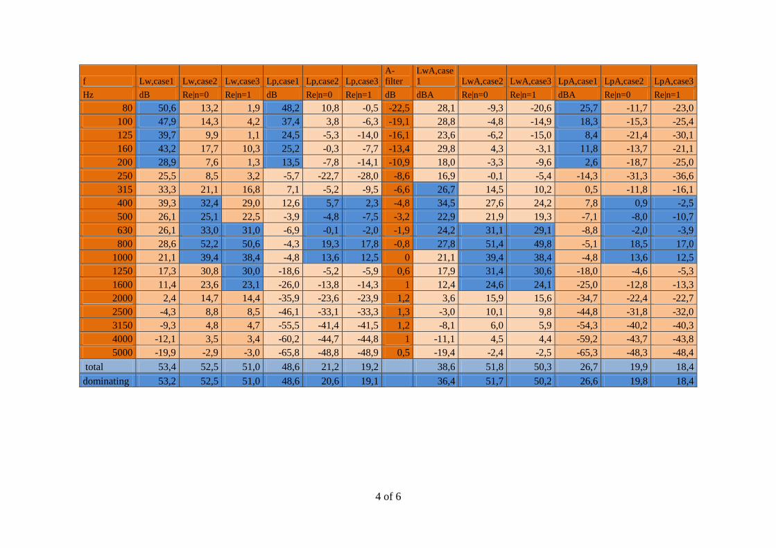
f Lw,case1 Lw,case2 Lw,case3 Lp,case1 Lp,case2 Lp,case3

A-

filter

LwA,case

1 LwA,case2 LwA,case3 LpA,case1 LpA,case2 LpA,case3

Hz dB Re|n=0 Re|n=1 dB Re|n=0 Re|n=1 dB dBA Re|n=0 Re|n=1 dBA Re|n=0 Re|n=1

80 50,6 13,2 1,9 48,2 10,8 -0,5 -22,5 28,1 -9,3 -20,6 25,7 -11,7 -23,0

100 47,9 14,3 4,2 37,4 3,8 -6,3 -19,1 28,8 -4,8 -14,9 18,3 -15,3 -25,4

125 39,7 9,9 1,1 24,5 -5,3 -14,0 -16,1 23,6 -6,2 -15,0 8,4 -21,4 -30,1

160 43,2 17,7 10,3 25,2 -0,3 -7,7 -13,4 29,8 4,3 -3,1 11,8 -13,7 -21,1

200 28,9 7,6 1,3 13,5 -7,8 -14,1 -10,9 18,0 -3,3 -9,6 2,6 -18,7 -25,0

250 25,5 8,5 3,2 -5,7 -22,7 -28,0 -8,6 16,9 -0,1 -5,4 -14,3 -31,3 -36,6

315 33,3 21,1 16,8 7,1 -5,2 -9,5 -6,6 26,7 14,5 10,2 0,5 -11,8 -16,1

400 39,3 32,4 29,0 12,6 5,7 2,3 -4,8 34,5 27,6 24,2 7,8 0,9 -2,5

500 26,1 25,1 22,5 -3,9 -4,8 -7,5 -3,2 22,9 21,9 19,3 -7,1 -8,0 -10,7

630 26,1 33,0 31,0 -6,9 -0,1 -2,0 -1,9 24,2 31,1 29,1 -8,8 -2,0 -3,9

800 28,6 52,2 50,6 -4,3 19,3 17,8 -0,8 27,8 51,4 49,8 -5,1 18,5 17,0

1000 21,1 39,4 38,4 -4,8 13,6 12,5 0 21,1 39,4 38,4 -4,8 13,6 12,5

1250 17,3 30,8 30,0 -18,6 -5,2 -5,9 0,6 17,9 31,4 30,6 -18,0 -4,6 -5,3

1600 11,4 23,6 23,1 -26,0 -13,8 -14,3 1 12,4 24,6 24,1 -25,0 -12,8 -13,3

2000 2,4 14,7 14,4 -35,9 -23,6 -23,9 1,2 3,6 15,9 15,6 -34,7 -22,4 -22,7

2500 -4,3 8,8 8,5 -46,1 -33,1 -33,3 1,3 -3,0 10,1 9,8 -44,8 -31,8 -32,0

3150 -9,3 4,8 4,7 -55,5 -41,4 -41,5 1,2 -8,1 6,0 5,9 -54,3 -40,2 -40,3

4000 -12,1 3,5 3,4 -60,2 -44,7 -44,8 1 -11,1 4,5 4,4 -59,2 -43,7 -43,8

5000 -19,9 -2,9 -3,0 -65,8 -48,8 -48,9 0,5 -19,4 -2,4 -2,5 -65,3 -48,3 -48,4

total 53,4 52,5 51,0 48,6 21,2 19,2 38,6 51,8 50,3 26,7 19,9 18,4

dominating 53,2 52,5 51,0 48,6 20,6 19,1 36,4 51,7 50,2 26,6 19,8 18,4

5 of 6

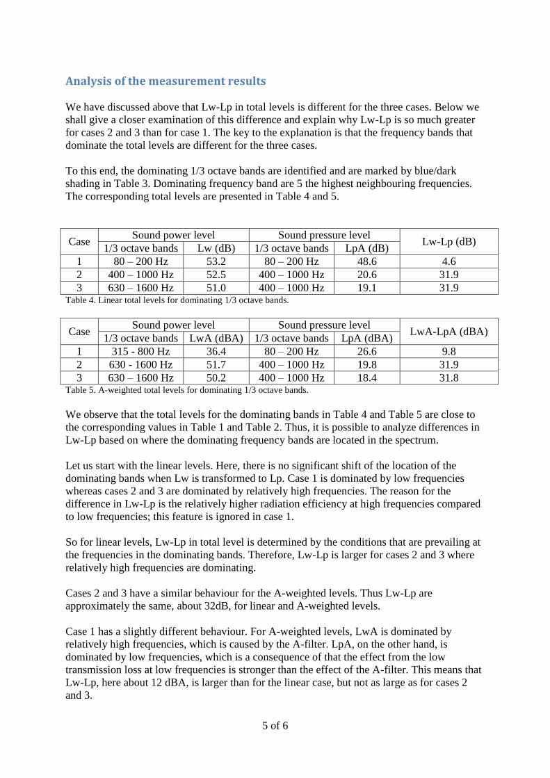
Analysis of the measurement results

We have discussed above that Lw-Lp in total levels is different for the three cases. Below we

shall give a closer examination of this difference and explain why Lw-Lp is so much greater

for cases 2 and 3 than for case 1. The key to the explanation is that the frequency bands that

dominate the total levels are different for the three cases.

To this end, the dominating 1/3 octave bands are identified and are marked by blue/dark

shading in Table 3. Dominating frequency band are 5 the highest neighbouring frequencies.

The corresponding total levels are presented in Table 4 and 5.

Case Sound power level Sound pressure level

Lw-Lp (dB) 1/3 octave bands Lw (dB) 1/3 octave bands LpA (dB)

1 80 – 200 Hz 53.2 80 – 200 Hz 48.6 4.6

2 400 – 1000 Hz 52.5 400 – 1000 Hz 20.6 31.9

3 630 – 1600 Hz 51.0 400 – 1000 Hz 19.1 31.9 Table 4. Linear total levels for dominating 1/3 octave bands.

Case Sound power level Sound pressure level

LwA-LpA (dBA) 1/3 octave bands LwA (dBA) 1/3 octave bands LpA (dBA)

1 315 - 800 Hz 36.4 80 – 200 Hz 26.6 9.8

2 630 - 1600 Hz 51.7 400 – 1000 Hz 19.8 31.9

3 630 – 1600 Hz 50.2 400 – 1000 Hz 18.4 31.8 Table 5. A-weighted total levels for dominating 1/3 octave bands.

We observe that the total levels for the dominating bands in Table 4 and Table 5 are close to

the corresponding values in Table 1 and Table 2. Thus, it is possible to analyze differences in

Lw-Lp based on where the dominating frequency bands are located in the spectrum.

Let us start with the linear levels. Here, there is no significant shift of the location of the

dominating bands when Lw is transformed to Lp. Case 1 is dominated by low frequencies

whereas cases 2 and 3 are dominated by relatively high frequencies. The reason for the

difference in Lw-Lp is the relatively higher radiation efficiency at high frequencies compared

to low frequencies; this feature is ignored in case 1.

So for linear levels, Lw-Lp in total level is determined by the conditions that are prevailing at

the frequencies in the dominating bands. Therefore, Lw-Lp is larger for cases 2 and 3 where

relatively high frequencies are dominating.

Cases 2 and 3 have a similar behaviour for the A-weighted levels. Thus Lw-Lp are

approximately the same, about 32dB, for linear and A-weighted levels.

Case 1 has a slightly different behaviour. For A-weighted levels, LwA is dominated by

relatively high frequencies, which is caused by the A-filter. LpA, on the other hand, is

dominated by low frequencies, which is a consequence of that the effect from the low

transmission loss at low frequencies is stronger than the effect of the A-filter. This means that

Lw-Lp, here about 12 dBA, is larger than for the linear case, but not as large as for cases 2

and 3.

6 of 6

Summary

In summary, the reason for the big difference for case 1 on one hand and cases 2 and 3 on the

other hand in Lw-Lp measured as total level, is the following. The radiation efficiency,

affecting both level and frequency spectrum, is ignored for case 1 whereas it is included in

cases 2 and 3.

School of Engineering 351 95 Växjö

tel 0772-28 80 00, fax 0470-76 85 40

estimate of cabin noise in an articulated hauler with...

Documents