estcp cost and performance report fileestcp cost and performance report environmental security...
TRANSCRIPT
ESTCPCost and Performance Report
ENVIRONMENTAL SECURITYTECHNOLOGY CERTIFICATION PROGRAM
U.S. Department of Defense
(CU-9603)
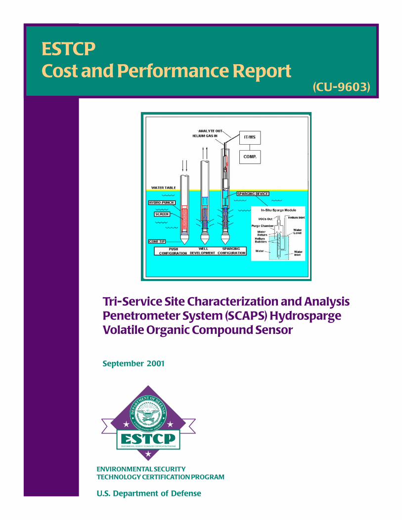
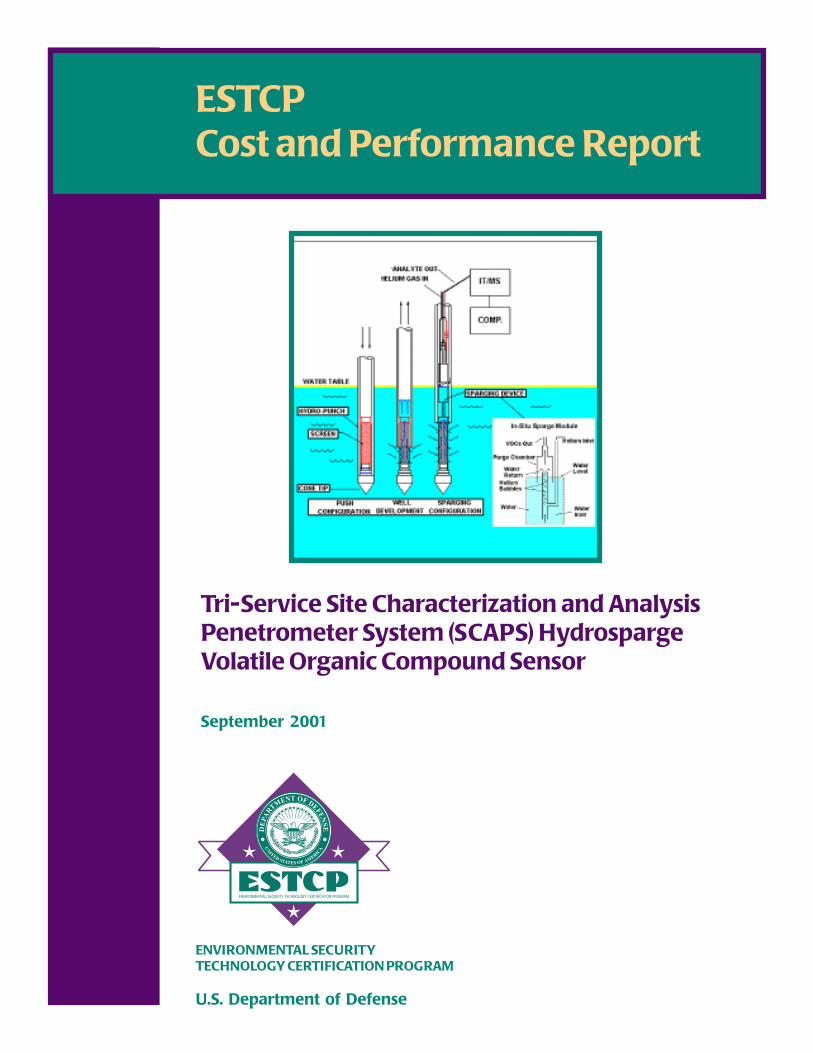
Tri-Service Site Characterization and AnalysisPenetrometer System (SCAPS) HydrospargeVolatile Organic Compound Sensor
September 2001
Tri-Service Site Characterization and AnalysisPenetrometer System (SCAPS) HydrospargeVolatile Organic Compound Sensor
September 2001
ESTCPCost and Performance Report
ENVIRONMENTAL SECURITYTECHNOLOGY CERTIFICATION PROGRAM
U.S. Department of Defense
i
TABLE OF CONTENTS
Page
1.0 INTRODUCTION . . . . . . . . . . . . . . . . . . . . . . . . . . . . . . . . . . . . . . . . . . . . . . . . . . . . . . . 1
2.0 TECHNOLOGY DESCRIPTION . . . . . . . . . . . . . . . . . . . . . . . . . . . . . . . . . . . . . . . . . . . 32.1 TECHNOLOGY BACKGROUND . . . . . . . . . . . . . . . . . . . . . . . . . . . . . . . . . . . . 3
2.1.1 SCAPS . . . . . . . . . . . . . . . . . . . . . . . . . . . . . . . . . . . . . . . . . . . . . . . . . . . . 42.1.2 Geophysical Cone Sensor . . . . . . . . . . . . . . . . . . . . . . . . . . . . . . . . . . . . . 52.1.3 In Situ Sparge Module . . . . . . . . . . . . . . . . . . . . . . . . . . . . . . . . . . . . . . . . 52.1.4 Direct Sampling Ion Trap Mass Spectrometer . . . . . . . . . . . . . . . . . . . . . 52.1.5 Quantitative Calibration of Hydrosparge Sensor . . . . . . . . . . . . . . . . . . . . 7
2.2 PERSONNEL TRAINING REQUIREMENTS . . . . . . . . . . . . . . . . . . . . . . . . . . 82.3 ADVANTAGES . . . . . . . . . . . . . . . . . . . . . . . . . . . . . . . . . . . . . . . . . . . . . . . . . . 82.4 LIMITS OF THE TECHNOLOGY . . . . . . . . . . . . . . . . . . . . . . . . . . . . . . . . . . . . 8
2.4.1 Truck-Mounted Cone Penetrometer Access Limits . . . . . . . . . . . . . . . . . 82.4.2 Cone Penetrometer Advancement Limits . . . . . . . . . . . . . . . . . . . . . . . . . 92.4.3 Extremely High Level Contamination Carry-Over . . . . . . . . . . . . . . . . . . 92.4.4 ITMS Limitations . . . . . . . . . . . . . . . . . . . . . . . . . . . . . . . . . . . . . . . . . . . 92.4.5 Direct Push Well Limitations . . . . . . . . . . . . . . . . . . . . . . . . . . . . . . . . . 10
3.0 DEMONSTRATION DESIGN . . . . . . . . . . . . . . . . . . . . . . . . . . . . . . . . . . . . . . . . . . . . 113.1 PREVIOUS DEMONSTRATIONS . . . . . . . . . . . . . . . . . . . . . . . . . . . . . . . . . . 11
3.1.1 Data Validation for Bush River Study Area, Aberdeen Proving Ground . . . . . . . . . . . . . . . . . . . . . . . . . . . . . . . . . . . . . . . . . . . . 11
3.1.2 Well Comparison Study at Davis Global Communication Site . . . . . . . . 113.1.3 Hydrosparge Data Collected at Fort Dix . . . . . . . . . . . . . . . . . . . . . . . . . 12
3.2 PERFORMANCE OBJECTIVES . . . . . . . . . . . . . . . . . . . . . . . . . . . . . . . . . . . . 123.2.1 Accuracy . . . . . . . . . . . . . . . . . . . . . . . . . . . . . . . . . . . . . . . . . . . . . . . . . 123.2.2 Time Required to Characterize Extent of Contamination . . . . . . . . . . . . 133.2.3 Reliability and Ruggedness . . . . . . . . . . . . . . . . . . . . . . . . . . . . . . . . . . . 13
3.3 PHYSICAL SETUP AND OPERATION . . . . . . . . . . . . . . . . . . . . . . . . . . . . . . 133.4 MONITORING PROCEDURES . . . . . . . . . . . . . . . . . . . . . . . . . . . . . . . . . . . . . 133.5 DEMONSTRATION SITE/FACILITY BACKGROUND . . . . . . . . . . . . . . . . . 143.6 DEMONSTRATION SITE/FACILITY CHARACTERISTICS . . . . . . . . . . . . . 16
3.6.1 Hydrogeology . . . . . . . . . . . . . . . . . . . . . . . . . . . . . . . . . . . . . . . . . . . . . 163.6.2 Extent of Contamination . . . . . . . . . . . . . . . . . . . . . . . . . . . . . . . . . . . . . 17
4.0 PERFORMANCE ASSESSMENT . . . . . . . . . . . . . . . . . . . . . . . . . . . . . . . . . . . . . . . . . 194.1 ACCURACY . . . . . . . . . . . . . . . . . . . . . . . . . . . . . . . . . . . . . . . . . . . . . . . . . . . . 194.2 TIME TO CHARACTERIZE EXTENT OF GROUNDWATER
CONTAMINATION . . . . . . . . . . . . . . . . . . . . . . . . . . . . . . . . . . . . . . . . . . . . . . 214.3 RELIABILITY AND RUGGEDNESS . . . . . . . . . . . . . . . . . . . . . . . . . . . . . . . . 23
ii
TABLE OF CONTENTS (continued)
Page
5.0 COST ASSESSMENT . . . . . . . . . . . . . . . . . . . . . . . . . . . . . . . . . . . . . . . . . . . . . . . . . . . 25
6.0 REFERENCES . . . . . . . . . . . . . . . . . . . . . . . . . . . . . . . . . . . . . . . . . . . . . . . . . . . . . . . . 27
APPENDIX A: Points of Contact . . . . . . . . . . . . . . . . . . . . . . . . . . . . . . . . . . . . . . . . . A-1
iii
LIST OF FIGURES
Page
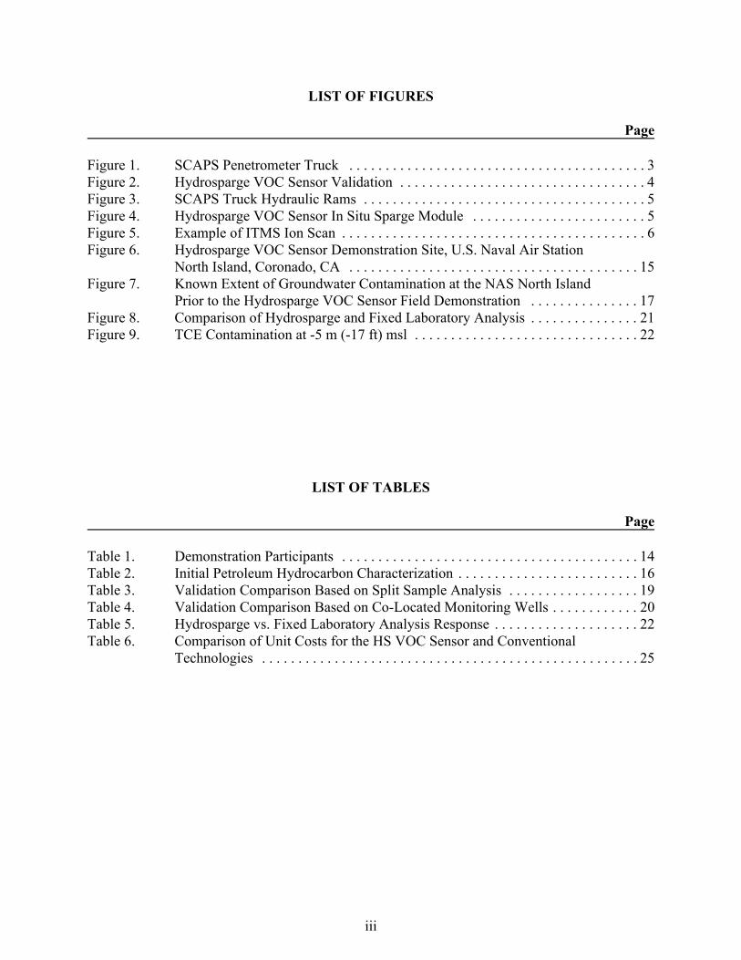
Figure 1. SCAPS Penetrometer Truck . . . . . . . . . . . . . . . . . . . . . . . . . . . . . . . . . . . . . . . . . 3Figure 2. Hydrosparge VOC Sensor Validation . . . . . . . . . . . . . . . . . . . . . . . . . . . . . . . . . . 4Figure 3. SCAPS Truck Hydraulic Rams . . . . . . . . . . . . . . . . . . . . . . . . . . . . . . . . . . . . . . . 5Figure 4. Hydrosparge VOC Sensor In Situ Sparge Module . . . . . . . . . . . . . . . . . . . . . . . . 5Figure 5. Example of ITMS Ion Scan . . . . . . . . . . . . . . . . . . . . . . . . . . . . . . . . . . . . . . . . . . 6Figure 6. Hydrosparge VOC Sensor Demonstration Site, U.S. Naval Air Station
North Island, Coronado, CA . . . . . . . . . . . . . . . . . . . . . . . . . . . . . . . . . . . . . . . . 15Figure 7. Known Extent of Groundwater Contamination at the NAS North Island
Prior to the Hydrosparge VOC Sensor Field Demonstration . . . . . . . . . . . . . . . 17Figure 8. Comparison of Hydrosparge and Fixed Laboratory Analysis . . . . . . . . . . . . . . . 21Figure 9. TCE Contamination at -5 m (-17 ft) msl . . . . . . . . . . . . . . . . . . . . . . . . . . . . . . . 22
LIST OF TABLES
Page
Table 1. Demonstration Participants . . . . . . . . . . . . . . . . . . . . . . . . . . . . . . . . . . . . . . . . . 14Table 2. Initial Petroleum Hydrocarbon Characterization . . . . . . . . . . . . . . . . . . . . . . . . . 16Table 3. Validation Comparison Based on Split Sample Analysis . . . . . . . . . . . . . . . . . . 19Table 4. Validation Comparison Based on Co-Located Monitoring Wells . . . . . . . . . . . . 20Table 5. Hydrosparge vs. Fixed Laboratory Analysis Response . . . . . . . . . . . . . . . . . . . . 22Table 6. Comparison of Unit Costs for the HS VOC Sensor and Conventional
Technologies . . . . . . . . . . . . . . . . . . . . . . . . . . . . . . . . . . . . . . . . . . . . . . . . . . . . 25
iv
LIST OF ACRONYMS
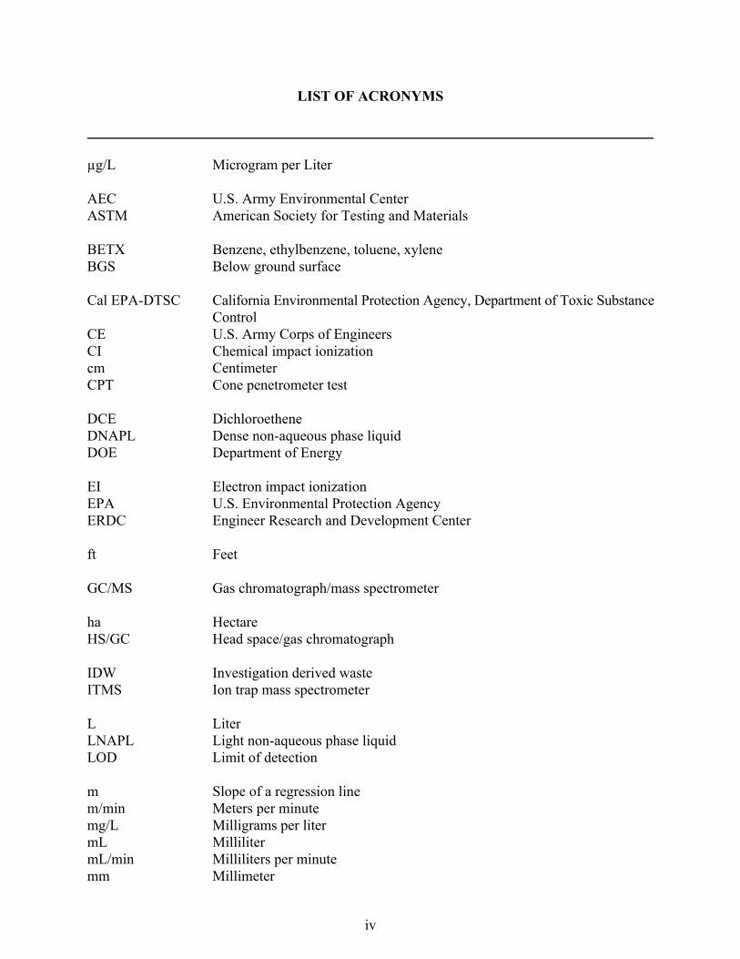
µg/L Microgram per Liter
AEC U.S. Army Environmental CenterASTM American Society for Testing and Materials
BETX Benzene, ethylbenzene, toluene, xyleneBGS Below ground surface
Cal EPA-DTSC California Environmental Protection Agency, Department of Toxic SubstanceControl
CE U.S. Army Corps of EngineersCI Chemical impact ionizationcm CentimeterCPT Cone penetrometer test
DCE DichloroetheneDNAPL Dense non-aqueous phase liquidDOE Department of Energy
EI Electron impact ionizationEPA U.S. Environmental Protection AgencyERDC Engineer Research and Development Center
ft Feet
GC/MS Gas chromatograph/mass spectrometer
ha HectareHS/GC Head space/gas chromatograph
IDW Investigation derived wasteITMS Ion trap mass spectrometer
L LiterLNAPL Light non-aqueous phase liquidLOD Limit of detection
m Slope of a regression linem/min Meters per minutemg/L Milligrams per litermL MillilitermL/min Milliliters per minutemm Millimeter
LIST OF ACRONYMS (continued)
v
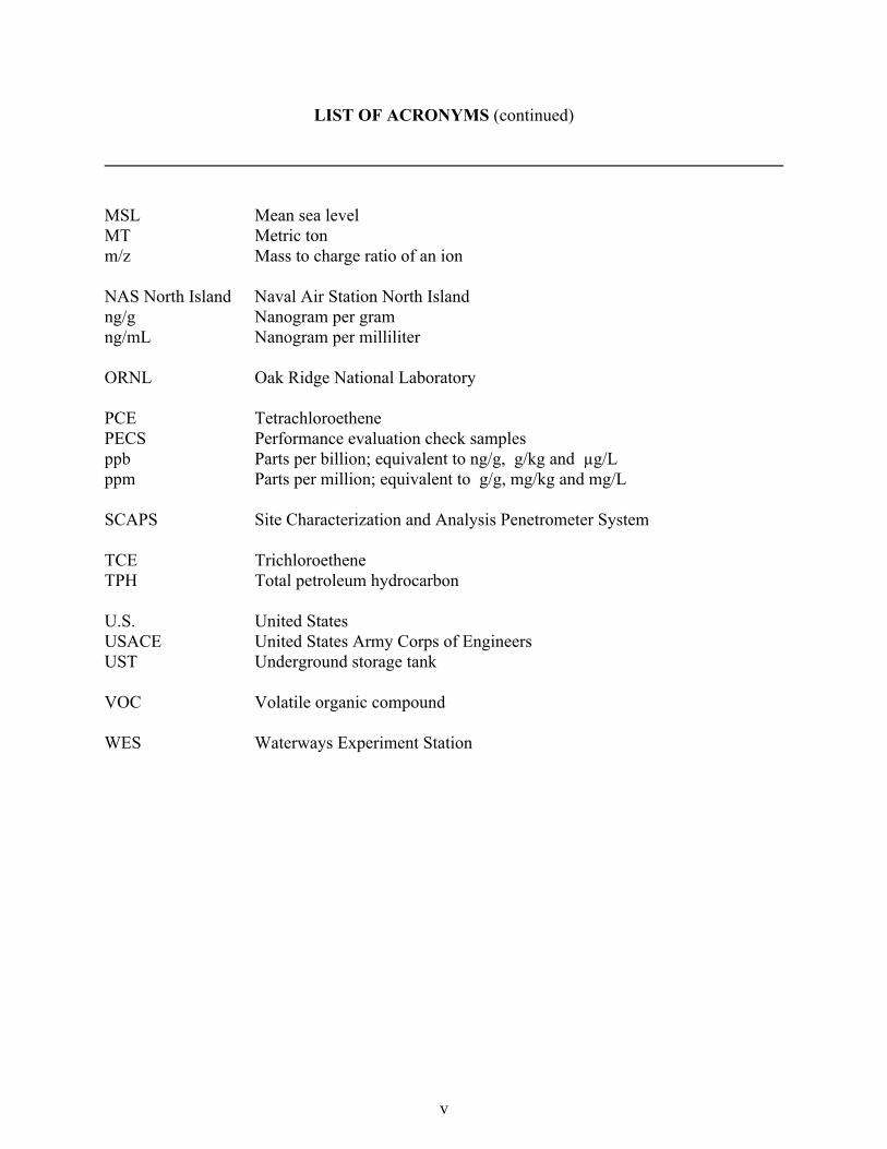
MSL Mean sea levelMT Metric tonm/z Mass to charge ratio of an ion
NAS North Island Naval Air Station North Islandng/g Nanogram per gramng/mL Nanogram per milliliter
ORNL Oak Ridge National Laboratory
PCE TetrachloroethenePECS Performance evaluation check samplesppb Parts per billion; equivalent to ng/g, g/kg and µg/Lppm Parts per million; equivalent to g/g, mg/kg and mg/L
SCAPS Site Characterization and Analysis Penetrometer System
TCE TrichloroetheneTPH Total petroleum hydrocarbon
U.S. United StatesUSACE United States Army Corps of EngineersUST Underground storage tank
VOC Volatile organic compound
WES Waterways Experiment Station
vi
ACKNOWLEDGMENTS
Several organizations and individuals cooperated to make this demonstration possible. Dr. JeffMarqusee of the Department of Defense Environmental Security Technology Certification Program(ESTCP) was instrumental in providing the funding for the technology performance evaluation. Mr.Richard Mach, Jr., of the Naval Facilities Engineering Command, Southwest Division, providedadditional funding and access to a challenging installation restoration site. Mr. George Robataillewas the technical monitor for the U.S. Army Environmental Center and Dr. M. John Cullinaneserved as Program Manager (PM) Environmental Restoration Research Program (EM-J), U.S. ArmyEngineer Research and Development Center (ERDC).
Personnel who cooperated in the execution of the study and the preparation of this report includedMr. Jed Costanza, Naval Facilities Engineering Service Center; Ms. Karen F. Myers, Environmentaland Molecular Chemistry Branch (EP-C), Environmental Engineering Division (EED),Environmental Laboratory (EL), ERDC; and Dr. William M. Davis, Environmental ProcessesBranch (EP-P), Environmental Processes and Engineering Division (EP), EL, ERDC. The authorsalso wish to acknowledge Mr. Jeff F. Powell and Mr. Dan Y. Eng, Information TechnologyLaboratory (ITL), ERDC, for technical assistance; Mr. Scott Morris, and Ms. Mery Coons of theOHM Remediation Services Corporation for assistance with site logistics and investigationmanagement; and Mr. Steve Brewer, Mr. Carl Sloan, Mr. Jeff Lacquement, Mr. Andy Mattioda, andMr. Eddie Mattioda, U.S. Army Engineer District, Tulsa, for operation of the SCAPS platform. Mr.Dan Y. Eng, ITL; Mr. Richard A. Karn, EP-C, EL; and Mr. John Ballard, EL, reviewed this report.
This report was prepared under the general supervision of Dr. Richard E. Price, Chief, EP; Ms.Denise MacMillan, Chief, EP-C; and Dr. John Keeley, Acting Director, EL.
At the time of publication of this report, Dr. James R. Houston was Director of ERDC, and Mr.Armando J. Roberto, Jr., was Acting Commander.
The contents of this report are not to be used for advertising, publication, or promotional purposes.Citation of trade names does not constitute an official endorsement or approval of the use of suchcommercial products.
Technical material contained in this report has been approved for public release.
1
1.0 INTRODUCTION
A July 1998 demonstration of the Hydrosparge volatile organic compound (VOC) sensor wasconducted at the Naval Air Station (NAS) North Island, Coronado, CA. The purpose was todemonstrate the ability of the Hydrosparge VOC sensor to characterize the extent of groundwatercontamination in a single field deployment and to evaluate the sensor with regard to the accuracyof analytical results, time required to characterize the extent of contamination, and the sensor'sreliability and ruggedness.
The Hydrosparge VOC sensor utilizes a commercially available direct push groundwater samplingtool to access groundwater. The in situ sparge module is then lowered directly into the groundwaterand purges VOC analytes in situ from the groundwater with helium gas bubbles. The volatilessparged from the water are carried via transfer tubing to a surface-deployed ion trap massspectrometer (ITMS) where the contaminants are analyzed in real-time. The analysis is performedin accordance with U.S. EPA draft Method 8265 (U.S. EPA 1994) to a detection limit ranging from1 to 5 ppb (µg/L).
A total of 115 groundwater samples collected from 50 locations were necessary to characterize theextent of contamination at the NAS North Island, Building 379 site. Eight conventionalgroundwater monitoring wells were installed after the Hydrosparge demonstration and the analysisof water samples collected from these wells verified the extent of contamination.
The Hydrosparge VOC sensor demonstration cost $158,173 for the collection and analysis of VOCsamples and the completion of 16 cone penetrometer soundings that provide continuous soillithology classification. A cost comparison between the actual costs of this demonstration and theestimated costs of completing a similar effort with monitoring wells showed that using theHydrosparge VOC sensor potentially saved $75,000. This equates to approximately a 32 percentcost savings. However, the Hydrosparge VOC sensor system provided onsite contaminantspeciation and quantification in near real-time. At the end of the demonstration, the site managerswere at a site restoration decision point that they may not have reached for several months ifconventional well installation, sampling, and offsite analysis techniques were used.
The time savings was made possible by completing the characterization during a single fieldinvestigation/demonstration. An experienced field crew that was allowed to make deploymentdecisions during the demonstration was responsible for this efficiency. The willingness of the sitemanagers to accommodate changes in the demonstration plan as sample analysis results becameavailable and more optimum locations for interrogation were identified also made this efficiencypossible.
The Hydrosparge VOC sensor is a quick and efficient tool used to screen a site for contaminationand to gain insight into the nature and extent of groundwater contamination. Groundwatermonitoring wells are essential for site verification and long-term monitoring. Both methods ofgroundwater interrogation are integral to cost-effective site remediation.

This page left blank intentionally.
3
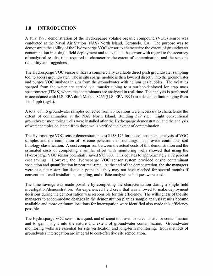
Figure 1. SCAPS Penetrometer Truck.
2.0 TECHNOLOGY DESCRIPTION
This section describes the Hydrosparge VOCsensor technology, a sensor which collects andanalyzes groundwater samples in the subsurfacesaturated zone. The sensor is deployed by aTri-Service Site Characterization and AnalysisPenetrometer System (SCAPS) (Figure 1).
2.1 TECHNOLOGY BACKGROUND
This technology was developed to address theneed to rapidly characterize chlorinated solventcontamination in groundwater at Department ofDefense (DoD) sites in a cost-effective manner.The Hydrosparge VOC sensor performs rapidfield screening to determine either the presenceor absence of volatile organic compound contaminants in subsurface media. In addition, theHydrosparge VOC sensor provides identification of specific analytes based on their mass spectraand provides estimates of contaminant concentrations.
The Hydrosparge VOC sensor utilizes a commercially available Hydropunch® or Powerpunch™direct push groundwater sampling tool to access the groundwater via temporary microwells. TheHydropunch is pushed to the desired depth and the push pipes are retracted, exposing the screenedinterval to the groundwater. The groundwater enters the microwell and is allowed to come toequilibrium, which generally takes less than 15 to 20 min.
The in situ sparge module, developed by the Department of Energy (DOE) Oak Ridge NationalLaboratory (ORNL), is then lowered into the microwell screen. The sparge module purges the VOCanalytes in situ from the groundwater using helium gas. The volatiles sparged from the water arecarried to an ITMS, where the contaminants are analyzed in near real-time. The analysis isperformed in accordance with EPA draft Method 8265, to a detection limit of the 1 to 5 ppb (µg/L)range.
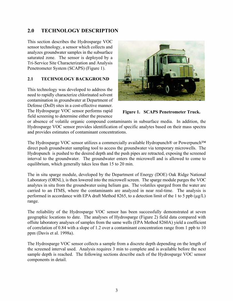
The reliability of the Hydrosparge VOC sensor has been successfully demonstrated at sevengeographic locations to date. The analyses of Hydrosparge (Figure 2) field data compared withoffsite laboratory analyses of samples from the same wells (EPA Method 8260A) yield a coefficientof correlation of 0.84 with a slope of 1.2 over a contaminant concentration range from 1 ppb to 10ppm (Davis et al. 1998a).
The Hydrosparge VOC sensor collects a sample from a discrete depth depending on the length ofthe screened interval used. Analysis requires 3 min to complete and is available before the nextsample depth is reached. The following sections describe each of the Hydrosparge VOC sensorcomponents in detail.
4
Figure 2. Hydrosparge VOC Sensor Validation.
2.1.1 SCAPS
The SCAPS is the result of a Tri-Service effort to utilize the capabilities of cone penetrometertechnology for characterizing subsurface contamination at military installations. Conepenetrometery has long been used to characterize soil for geotechnical parameters such as soilstrength and liquefaction potential. This is accomplished by advancing (pushing) a standard conepenetrometer probe into the ground by hydraulic ram force.
The SCAPS truck is a standard 18.2 MT (20-ton) mobile cone penetrometer testing (CPT) platformused to advance contaminant and geotechnical sensing probes. The forward portion of the SCAPStruck houses the hydraulic rams (Figure 3) used to translate the weight of the truck (reaction mass)into pushing force. The combination of reaction mass and hydraulics can advance a 1-m-long by3.57-cm-diameter steel rod into the ground at a rate of 1 m/min in accordance with AmericanSociety of Testing and Materials (ASTM) Method D3441 (ASTM 1991), the standard forgeophysical sensing CPT. The rods, various sensing probes, or sampling tools can be advanced todepths in excess of 50 m (164 ft) in nominally compacted soils. Some SCAPS sensor probes areconfigured with retraction grouting capability. As the rods are withdrawn, a sacrificial cone tip isejected and grout is transferred from a surface mounted grout pumping station through 6.35-mm-(0.25-in.-) diameter tubing within the SCAPS probe umbilical cables, and is injected hydraulicallyto seal the penetrometer hole. Also, while the rods are withdrawn, they are cleaned within a hot
5
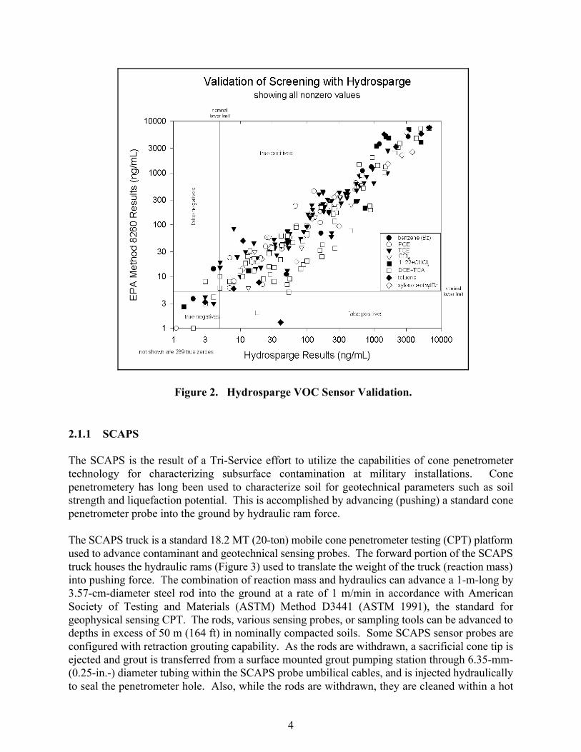
Figure 3. SCAPS TruckHydraulic Rams.
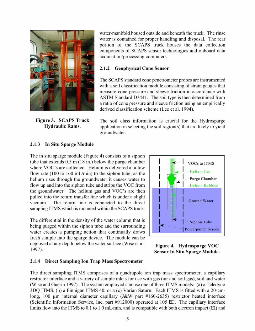
Figure 4. Hydrosparge VOCSensor In Situ Sparge Module.
water-manifold housed outside and beneath the truck. The rinsewater is contained for proper handling and disposal. The rearportion of the SCAPS truck houses the data collectioncomponents of SCAPS sensor technologies and onboard dataacquisition/processing computers.
2.1.2 Geophysical Cone Sensor
The SCAPS standard cone penetrometer probes are instrumentedwith a soil classification module consisting of strain gauges thatmeasure cone pressure and sleeve friction in accordance withASTM Standard D3441. The soil type is then determined froma ratio of cone pressure and sleeve friction using an empiricallyderived classification scheme (Lee et al. 1994).
The soil class information is crucial for the Hydrospargeapplication in selecting the soil region(s) that are likely to yieldgroundwater.
2.1.3 In Situ Sparge Module
The in situ sparge module (Figure 4) consists of a siphontube that extends 0.5 m (18 in.) below the purge chamberwhere VOC’s are collected. Helium is delivered at a lowflow rate (100 to 160 mL/min) to the siphon tube; as thehelium rises through the groundwater it causes water toflow up and into the siphon tube and strips the VOC fromthe groundwater. The helium gas and VOC’s are thenpulled into the return transfer line which is under a slightvacuum. The return line is connected to the directsampling ITMS which is mounted within the SCAPS truck.
The differential in the density of the water column that isbeing purged within the siphon tube and the surroundingwater creates a pumping action that continually drawsfresh sample into the sparge device. The module can bedeployed at any depth below the water surface (Wise et al.1997).
2.1.4 Direct Sampling Ion Trap Mass Spectrometer
The direct sampling ITMS comprises of a quadrupole ion trap mass spectrometer, a capillaryrestrictor interface and a variety of sample inlets for use with gas (air and soil gas), soil and water(Wise and Guerin 1997). The system employed can use one of three ITMS models: (a) a Teledyne3DQ ITMS, (b) a Finnigan ITMS 40, or a (c) Varian Saturn. Each ITMS is fitted with a 20-cm-long, 100 µm internal diameter capillary (J&W part #160-2635) restrictor heated interface(Scientific Information Service, Inc. part #912000) operated at 105 EC. The capillary interfacelimits flow into the ITMS to 0.1 to 1.0 mL/min, and is compatible with both electron impact (EI) and
6
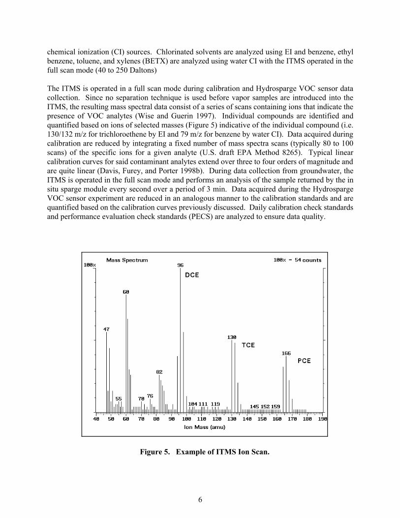
Figure 5. Example of ITMS Ion Scan.
chemical ionization (CI) sources. Chlorinated solvents are analyzed using EI and benzene, ethylbenzene, toluene, and xylenes (BETX) are analyzed using water CI with the ITMS operated in thefull scan mode (40 to 250 Daltons)
The ITMS is operated in a full scan mode during calibration and Hydrosparge VOC sensor datacollection. Since no separation technique is used before vapor samples are introduced into theITMS, the resulting mass spectral data consist of a series of scans containing ions that indicate thepresence of VOC analytes (Wise and Guerin 1997). Individual compounds are identified andquantified based on ions of selected masses (Figure 5) indicative of the individual compound (i.e.130/132 m/z for trichloroethene by EI and 79 m/z for benzene by water CI). Data acquired duringcalibration are reduced by integrating a fixed number of mass spectra scans (typically 80 to 100scans) of the specific ions for a given analyte (U.S. draft EPA Method 8265). Typical linearcalibration curves for said contaminant analytes extend over three to four orders of magnitude andare quite linear (Davis, Furey, and Porter 1998b). During data collection from groundwater, theITMS is operated in the full scan mode and performs an analysis of the sample returned by the insitu sparge module every second over a period of 3 min. Data acquired during the HydrospargeVOC sensor experiment are reduced in an analogous manner to the calibration standards and arequantified based on the calibration curves previously discussed. Daily calibration check standardsand performance evaluation check standards (PECS) are analyzed to ensure data quality.
7
Dynamic range. The linear dynamic range of the SCAPS Hydrosparge VOC sensor depends onthe dynamic range of the ITMS. Previous investigations using the ITMS have found that the linearportion of the response curves extends well beyond three orders of magnitude from low microgramsper liter (parts per billion) to milligrams per liter (parts per million) (Davis, Furey, and Porter1998b). Nonlinearity tends to occur at concentrations greater than tens of milligrams per liter inwater. The linear dynamic range of the ITMS also depends on operator-controlled instrumentalparameters. The linear dynamic range may be extended to higher concentrations by adjusting theionization time of the ITMS detector, but this results in decreased sensitivity at lower concentrations.
System limit of detection. Three quantities are needed to determine the Hydrosparge systemsdetection limits: electronic noise, background, and sensitivity. As with the linear dynamic range,these three parameters are related to the ITMS. These quantities are determined using the calibrationsamples prepared immediately prior to the site visit and standard analytical techniques (U.S. EPA1993; Davis, Furey, and Porter 1998b).
Limits of detection (LOD) were calculated according to the method outlined in SW 846 (USEPA1993). This method involves n replicate measurements of a low but detectable analyteconcentration, estimation of analytical system noise as the variance of the n replicate measurements,and calculating the LOD using the following equation:
LOD = t Sn-1, α/s
where t is the student t value for n replicates at the 95 percent confidence level and S estimaten-1, α/sof the standard deviation. For n values between 5 and 9, the t ranges between 2.78 and 2.23.n-1,α/sMeasurements for LOD calculations are made using the entire Hydrosparge VOC sensing system;therefore, measuring the expected overall system performance during the in situ application. TypicalLOD values calculated for data obtained in actual field operations are consistently single µg/L. TheSCAPS Hydrosparge VOC sensor detection limits will vary somewhat from site to site, but is in therange of 2 to 5 µg/L for the 34 VOC analytes listed on the EPA Target Compound List.
2.1.5 Quantitative Calibration of Hydrosparge Sensor
The ITMS, like any other analytical instrument, provides an intensity response relative to the amountof contaminant present in the sample analyzed. The ITMS does not directly provide theconcentration of the contaminant in the sample. To estimate the concentration present in the fieldsample, a series of analytical standards spiked with known quantities of contaminant are analyzedby the instrument and a calibration curve is generated. The actual concentration value can never beknown and is always an estimate.
The in situ sparge module and ITMS are calibrated by spiking a 250 mL volumetric flask containingdistilled water and a known concentration of analytes. The sparge module is inserted into the flask,the helium flow rate is adjusted at the beginning of the calibration (generally between 100 and 160mL/min) and remains constant during calibration and Hydrosparge in situ sample collection andanalysis. The calibration procedure is conducted under the same operating conditions used duringthe Hydrosparge field operation.
8
2.2 PERSONNEL TRAINING REQUIREMENTS
Personnel operating the SCAPS CPT platform should be trained in the installation of groundwatermonitoring wells and other traditional drilling methods. Operators of the ITMS vary in skill andtraining but should be experienced in the operation of standard laboratory equipment. All personneloperating the Hydrosparge direct sampling ITMS should be familiar with the operation of computersoftware and should be familiar with safety requirements for working around heavy equipment.Other than yearly Hazardous Waste Worker Update Training requirements, there is no mandatedtraining required to operate the CPT or the ITMS during field investigations.
2.3 ADVANTAGES
The SCAPS Hydrosparge VOC sensor is an in situ field screening device for characterizing thesubsurface distribution of volatile organic compound contamination without the installation ofconventional groundwater monitoring wells. The method is not intended to be a completereplacement for traditional monitoring wells, but is a means to optimize the placement of monitoringwells and usually results in the placement of a reduced number of monitoring wells to achieve sitecharacterization and/or long-term monitoring.
The Hydrosparge VOC sensor uses a CPT platform to provide near real-time field screening of thedistribution of VOC contamination at hazardous waste sites. The current configuration is designedto quickly and cost-effectively distinguish VOC contaminated areas from uncontaminated areas andto provide semiquantitative estimates of groundwater VOC contaminant concentrations. Thiscapability allows further investigation and remediation decisions to be made more efficiently andreduces the number of samples that must be submitted to laboratories for costly and time-consuminganalysis. In addition, the SCAPS CPT platform allows for the characterization of contaminated siteswith minimal exposure of site personnel and the community to toxic contaminants, and minimizesthe volume of investigation derived waste (IDW) generated during conventional drill/sample sitecharacterization activities.
2.4 LIMITS OF THE TECHNOLOGY
This section discusses the limits of the SCAPS Hydrosparge VOC sensor as they are currentlyunderstood.
2.4.1 Truck-Mounted Cone Penetrometer Access Limits
The SCAPS CPT vehicle is an 18.2 MT (20-ton) push platform built on a commercially availablediesel-powered truck chassis. The dimensions of the truck require a minimum access width of 3 m(10 ft) and a height clearance of 4.6 m (15 ft). It is conceivable that some sites, or certain areas ofsites, might not be accessible to a vehicle the size of the SCAPS CPT truck. The access limits forthe SCAPS CPT vehicle are similar to those for conventional drill rigs and heavy excavationequipment. However, the Hydrosparge VOC sensor can be run out of the back of a van withgroundwater accessed by smaller direct push rigs.
9
2.4.2 Cone Penetrometer Advancement Limits
The CPT sensors and sampling tools may be difficult to advance in subsurface lithologies containingcemented sands and clays, buried debris, gravel units, cobbles, boulders, and shallow bedrock. Aswith all intrusive site characterization methods, it is extremely important that all undergroundutilities and structures be located using reliable geophysical equipment operated by trainedprofessionals before penetrometer activities are initiated. This should be done even if subsurfaceutility plans for the site are available for reference.
2.4.3 Extremely High Level Contamination Carry-Over
The effective dynamic range for the Hydrosparge VOC sensor is determined by two factors: thedynamic range of the ITMS (discussed previously) and the potential for carry-over or crosscontamination of the in situ sparge module and analyte transfer line. All analytical systems haveupper limits of detection as well as lower limits of detection. The upper limit of detection for theITMS is determined by the number of molecules that it can analyze before the detector is "saturated"with ions (Wise and Guerin 1997). However, it is the internal contamination of the transfer linesthat often determine the lower limit of detection.
Extremely high levels of subsurface VOC contamination will cause carry- over of analytes betweensuccessive runs. That is, after sampling a high contaminant concentration, residual VOC analytesmay remain in the sampler transfer lines. This is considered sample carry-over between runs. Thisproblem cannot be completely eliminated, but the effects of residual sample carry-over can becontrolled. After an extremely high level sample has been analyzed, a system blank is analyzed.Residual sample carry-over is observed when VOC analytes are detected in blank samples abovethe system background response. When residual sample carry-over is detected, the sample transferlines are replaced and the contaminated lines are left to purge with helium gas for approximately 30min. Thus, by using two interchangeable in situ sparge modules and transfer lines, there is no lostproduction time.
2.4.4 ITMS Limitations
The ITMS is operated as the detector for the Hydrosprage VOC sensor as detailed in EPA draftMethod 8265 and as described in Davis, Furey, and Porter (1998b). This method is intended forfield screening applications via direct sampling ITMS. One of the limitations of the ITMS is theinability of the ITMS to distinguish between analyte pairs that yield identical mass fragments. Forexample, 1,1,2,2 tetrachloroethane and chloroform (trichloromethane) yield ions primarily at masses83 and 85. Using the current ITMS technology it is not possible to differentiate these two analytes;therefore they are reported as a sum of the two analytes. It should be noted that the current EPAlaboratory method (EPA Method 8260) using gas chromatography/mass spectrometry is also notable to differentiate some analyte pairs such as meta and para-xylene. Nevertheless, even whensamples are contaminated with complex mixtures of analytes, the ITMS can usually provide a usefullevel of qualitative and quantitative contaminant screening information.
10
2.4.5 Direct Push Well Limitations
Direct push microwells have many of the same limitations that conventional monitoring wells have:difficulty obtaining water samples from low conductivity soils, difficulty with installation in flowingsands, and the potential for spreading contamination during installation.
Currently, during the water access phase of the Hydrosparge operation, the direct push well isinstalled without casing to minimize expense of operation. Without casing to prevent movement ofcontaminants in the annulus, there is an increased potential for cross layer contamination. Aquitardsand isolating lithologies that separate contaminated regions should not be breached.
The NAS North Island site has a suspected low permeability layer at 13.7 m (45 ft) below groundsurface (BGS) which was never breached during the investigation.
11
3.0 DEMONSTRATION DESIGN
This section discusses the technology claims, demonstration objectives, sampling design, and dataanalysis protocols that will be used to evaluate the results of the demonstration.
3.1 PREVIOUS DEMONSTRATIONS
The HS VOC sensor technology was previously demonstrated under this program at three sites:
a. Bush River Study Area, U.S. Army Aberdeen Proving Ground, Edgewood, MD; June andAugust 1996.
b. Davis Global Communication Site, McClellan Air Force Base, Sacramento, CA; November1996 and February 1997.
c. U.S. Army Fort Dix, NJ; June and July 1997.
While the data were not used in this demonstration report, each site and its results are discussedbriefly in the following paragraphs.
3.1.1 Data Validation for Bush River Study Area, Aberdeen Proving Ground
The validation sample results from the HS VOC sensor demonstration performed at Bush RiverStudy Area (BRSA) during June 1996 indicated that the HS VOC Sensor was underestimating theVOC concentrations when compared with the verification samples measured by EPA Method 8260.The data collected during the June demonstration were collected using a Teledyne DSITMS. Inmid-August, the ERDC-WES SCAPS team performed additional HS VOC Sensor penetrations atthe BRSA to identify the source of the low bias provided by the Teledyne DSITMS. This work wasconducted using a Finnigan ITMS 40 and the results were compared with data collected using theTeledyne DSITMS. This comparison indicated that the Teledyne did yield a low bias for high VOCconcentrations. It should be noted that the bias was only observed at concentrations > 1,000 µg/L.The instrumental bias was not detected during previous field operations since that the highestconcentration PE check standard analyzed was 50 µg/L. All subsequent HS VOC sensordemonstrations incorporated higher concentration PE check standards.
The source of the bias in the Teledyne data appeared to be due to a thermal cold spot in the DSITMSheated inlet where the helium purge gas from the in situ purge module entered the DSITMS. Thecold spot was brought to the attention of the Teledyne manufacturer and the problem was corrected.
Based on problems encountered with the Teledyne DSITMS, only the data collected using theFinnigan DSITMS were used for data comparisons between the HS VOC sensor and the validationsamples analyzed using EPA Method 8260. Linear regression statistics of the BRSA data show acorrelation of 0.63 and a slope of 1.2.
3.1.2 Well Comparison Study at Davis Global Communication Site
At the Davis Global Communication Site (DGCS), HS VOC sensor data were compared toconventional, established monitoring wells and to groundwater from the direct push wells. Resultsfrom the demonstration indicate, regardless of the source of water (direct push miniwell, or
12
conventional monitoring well), that the in situ sparge/DSITMS measurement of the groundwaterVOC concentrations are comparable to measurements made by offsite sample analyses using EPAMethod 8260. Correlations between the Hydrosparge data and conventional EPA Method 8260 datafrom existing monitoring wells, however, showed a definite low bias. Experiments involvingclustering direct push wells at different depths around existing monitoring wells were conducted todetermine the cause of this bias. Using the HS VOC sensor along with the Thermal DesorptionVOC Sampler, it was demonstrated that the wells at DGCS had been improperly designed allowinguncontaminated groundwater to leach contaminants from the contaminated clay-confining layer intothe groundwater.
Since the low bias for the data was explained, the comparison of the HS VOC data to existingmonitoring well data was omitted from the DGCS data comparison. Linear regression statistics forthe direct push groundwater comparison of the Hydrosparge /DSITMS data to conventional EPAmethod 8260 data show a correlation of 0.88 with a slope on 1.1.
3.1.3 Hydrosparge Data Collected at Fort Dix
All Hydrosparge in situ and verification data collection activities at the Fort Dix demonstration wereconducted as planned. No problems were encountered with either the HS VOC sensor or theHydrosparge/conventional well comparison study. Linear regression statistics show a correlationof 0.85 and a slope of 1.2.
3.2 PERFORMANCE OBJECTIVES
This technology was developed to address the need to rapidly characterize chlorinated solventcontamination in groundwater to a degree of precision that is economically feasible. Therefore theHydrosparge VOC sensor should not only approach the accuracy of traditional sample collectionand analysis techniques, but also should be able to complete contaminant characterization in lesstime at a significantly lower cost. With this claim in mind the SCAPS Hydrosparge VOC sensorperformance will be compared to conventional sampling and analytical methods for:
a. Accuracy of analytical result.b. Time required to characterize extent of contamination.c. Reliability and ruggedness.
3.2.1 Accuracy
As part of the objectives outlined above, the SCAPS Hydrosparge VOC sensor was evaluated todetermine agreement between data produced in situ and the results of laboratory verification sampleanalyses by EPA Method 8260A. The Hydrosparge VOC sensor detection limit was determinedaccording to EPA draft Method 8265 procedures. When the ITMS response exceeded the detectionlimit, the data were considered to be a “detect.” The detection limit for the verification samples wasdetermined by an offsite independent laboratory using EPA Method 8260A.
The Hydrosparge VOC sensor produced data that were reduced to concentration units of µg/L.These are the same data type and concentration units used for reporting data from the verificationmethod (EPA Method 8260A). Hence, direct comparison of the SCAPS Hydrosparge VOC sensoranalysis results with those from the verification sample analyses was simple and straightforward.
13
The strength of comparisons between the Hydrosparge VOC sensor data and the conventionalmethods of analysis for verification samples was evaluated using least squares linear regression overthe entire concentration range of data collected. The Hydrosparge VOC sensor analysis results andconventional analysis results were considered to strongly agree if the correlation coefficient of thelinear regression was 1.0 ± 0.2 and the slope of the regression line was 1.0 ± 0.2. Previous fielddemonstrations of the Hydrosparge VOC sensor indicate strong correlations between in situ analysisresults and EPA Method 8260A analysis of verification samples (Davis et al. 1998a).
3.2.2 Time Required to Characterize Extent of Contamination
Field implementation of conventional characterization technology is typically a rigid process. Oncethe sample collection locations are chosen they are not changed while the sampling crew is in thefield. The lapse of time between collecting samples and receiving a report detailing the sampleanalysis results is nominally 6 months to a year. Once the analysis results are available they usuallyreveal that more samples are required before remediation decisions can be made. Another lapse intime occurs in completing contractual details to prepare sample collection plans. Yet another lapsein time occurs in completing contractual details to implement the sampling plans. These time lapsescan easily exceed a year. An objective of this demonstration was to characterize the extent ofchlorinated solvent contamination in a single field deployment.
3.2.3 Reliability and Ruggedness
The reliability of the Hydrosparge VOC sensor is a measure of how many consistent days samplecollection and analysis occurs. Ruggedness refers to physical, thermal, and chemical shocksendured by the sensor that do not interfere with repeatability of measurements.
3.3 PHYSICAL SETUP AND OPERATION
The demonstration was conducted July 1998. The goal to characterize the extent of contaminationin one field deployment required the close cooperation of a variety of people. Table 1 provides thepartnered organizations and their respective responsibilities.
3.4 MONITORING PROCEDURES
Monitoring the Hydrosparge VOC sensor performance consisted of quality assurance checks andindependent analysis of verification sample analysis. Method Blanks (consisting of reagent water)were analyzed at the beginning of each work day to document system background and to insure thatresidual VOC contaminants were purged from the Hydrosparge VOC sensor system. Triplicatecalibration samples of a single known concentration were analyzed at the beginning of each workingday (daily calibration check standards). In addition, a single calibration check sample of knownconcentration was analyzed immediately prior to in situ Hydrosparge VOC sensor data collection.Once daily, an externally prepared calibration check standard was analyzed to evaluate the accuracyof the working calibration stock solution and continuing calibration.
14
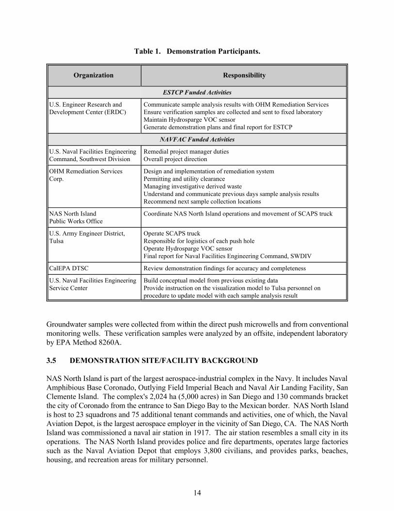
Table 1. Demonstration Participants.
Organization Responsibility
ESTCP Funded Activities
U.S. Engineer Research and Communicate sample analysis results with OHM Remediation ServicesDevelopment Center (ERDC) Ensure verification samples are collected and sent to fixed laboratory
Maintain Hydrosparge VOC sensorGenerate demonstration plans and final report for ESTCP
NAVFAC Funded Activities
U.S. Naval Facilities Engineering Remedial project manager dutiesCommand, Southwest Division Overall project direction
OHM Remediation Services Design and implementation of remediation systemCorp. Permitting and utility clearance
Managing investigative derived wasteUnderstand and communicate previous days sample analysis resultsRecommend next sample collection locations
NAS North Island Coordinate NAS North Island operations and movement of SCAPS truckPublic Works Office
U.S. Army Engineer District, Operate SCAPS truckTulsa Responsible for logistics of each push hole
Operate Hydrosparge VOC sensorFinal report for Naval Facilities Engineering Command, SWDIV
CalEPA DTSC Review demonstration findings for accuracy and completeness
U.S. Naval Facilities Engineering Build conceptual model from previous existing dataService Center Provide instruction on the visualization model to Tulsa personnel on
procedure to update model with each sample analysis result
Groundwater samples were collected from within the direct push microwells and from conventionalmonitoring wells. These verification samples were analyzed by an offsite, independent laboratoryby EPA Method 8260A.
3.5 DEMONSTRATION SITE/FACILITY BACKGROUND
NAS North Island is part of the largest aerospace-industrial complex in the Navy. It includes NavalAmphibious Base Coronado, Outlying Field Imperial Beach and Naval Air Landing Facility, SanClemente Island. The complex's 2,024 ha (5,000 acres) in San Diego and 130 commands bracketthe city of Coronado from the entrance to San Diego Bay to the Mexican border. NAS North Islandis host to 23 squadrons and 75 additional tenant commands and activities, one of which, the NavalAviation Depot, is the largest aerospace employer in the vicinity of San Diego, CA. The NAS NorthIsland was commissioned a naval air station in 1917. The air station resembles a small city in itsoperations. The NAS North Island provides police and fire departments, operates large factoriessuch as the Naval Aviation Depot that employs 3,800 civilians, and provides parks, beaches,housing, and recreation areas for military personnel.
15
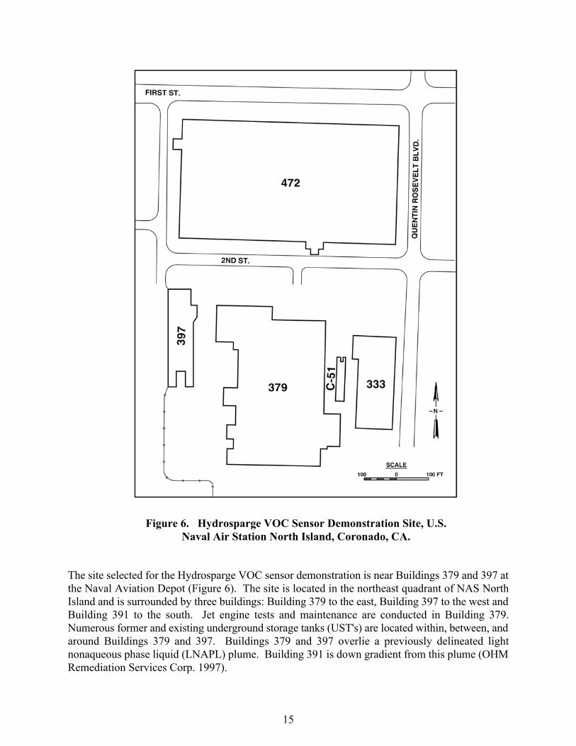
Figure 6. Hydrosparge VOC Sensor Demonstration Site, U.S.Naval Air Station North Island, Coronado, CA.
The site selected for the Hydrosparge VOC sensor demonstration is near Buildings 379 and 397 atthe Naval Aviation Depot (Figure 6). The site is located in the northeast quadrant of NAS NorthIsland and is surrounded by three buildings: Building 379 to the east, Building 397 to the west andBuilding 391 to the south. Jet engine tests and maintenance are conducted in Building 379.Numerous former and existing underground storage tanks (UST's) are located within, between, andaround Buildings 379 and 397. Buildings 379 and 397 overlie a previously delineated lightnonaqueous phase liquid (LNAPL) plume. Building 391 is down gradient from this plume (OHMRemediation Services Corp. 1997).
16
3.6 DEMONSTRATION SITE/FACILITY CHARACTERISTICS
Petroleum hydrocarbon characterization efforts prior to this demonstration are summarized in Table2. Initial site assessment of potential leaks for USTs was conducted by Jacobs Engineering GroupInc. in 1991. Seven soil borings and three monitoring wells indicated contamination in the areaaround and below the buildings. Contamination was identified by measuring total petroleumhydrocarbons (TPH) in soil and benzene in groundwater. Free product LNAPL was detected in oneof the initial three monitoring wells. Based on the initial results, Geosciences conducted further siteassessment during 1993. Ten soil borings and nine monitoring wells were installed and sampled.The TPH laboratory tests identified contamination in many of the soil boring samples and LNAPLwas detected in two of the monitoring wells (OHM Remediation Services Corp. 1997).
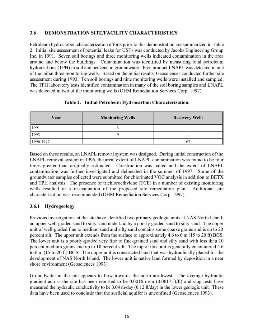
Table 2. Initial Petroleum Hydrocarbon Characterization.
Year Monitoring Wells Recovery Wells
1991 3 --
1993 9 --
1996-1997 -- 67
Based on these results, an LNAPL removal system was designed. During initial construction of theLNAPL removal system in 1996, the areal extent of LNAPL contamination was found to be fourtimes greater than originally estimated. Construction was halted and the extent of LNAPLcontamination was further investigated and delineated in the summer of 1997. Some of thegroundwater samples collected were submitted for chlorinated VOC analysis in addition to BETXand TPH analysis. The presence of trichloroethylene (TCE) in a number of existing monitoringwells resulted in a re-evaluation of the proposed site remediation plan. Additional sitecharacterization was recommended (OHM Remediation Services Corp. 1997).
3.6.1 Hydrogeology
Previous investigations at the site have identified two primary geologic units at NAS North Island:an upper well-graded sand to silty sand underlaid by a poorly graded sand to silty sand. The upperunit of well-graded fine to medium sand and silty sand contains some coarse grains and is up to 20percent silt. The upper unit extends from the surface to approximately 4.6 to 6 m (15 to 20 ft) BGS.The lower unit is a poorly-graded very fine to fine-grained sand and silty sand with less than 10percent medium grains and up to 10 percent silt. The top of this unit is generally encountered 4.6to 6 m (15 to 20 ft) BGS. The upper unit is constructed land that was hydraulically placed for thedevelopment of NAS North Island. The lower unit is native land formed by deposition in a nearshore environment (Geosciences 1993).
Groundwater at the site appears to flow towards the north-northwest. The average hydraulicgradient across the site has been reported to be 0.0016 m/m (0.0017 ft/ft) and slug tests havemeasured the hydraulic conductivity to be 0.04 m/day (0.12 ft/day) in the lower geologic unit. Thesedata have been used to conclude that the surficial aquifer is unconfined (Geosciences 1993).
17
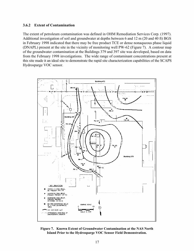
Figure 7. Known Extent of Groundwater Contamination at the NAS NorthIsland Prior to the Hydrosparge VOC Sensor Field Demonstration.
3.6.2 Extent of Contamination
The extent of petroleum contamination was defined in OHM Remediation Services Corp. (1997).Additional investigation of soil and groundwater at depths between 6 and 12 m (20 and 40 ft) BGSin February 1998 indicated that there may be free product TCE or dense nonaqueous phase liquid(DNAPL) present at the site in the vicinity of monitoring well PW-62 (Figure 7). A contour mapof the groundwater contamination at the Buildings 379 and 397 site was developed, based on datafrom the February 1998 investigations. The wide range of contaminant concentrations present atthis site made it an ideal site to demonstrate the rapid site characterization capabilities of the SCAPSHydrosparge VOC sensor.

This page left blank intentionally.
19
4.0 PERFORMANCE ASSESSMENT
Determination of the SCAPS Hydrosparge VOC sensor performance was in comparison toconventional sampling and analytical methods. Three specific criteria for comparison were:
a. Accuracy of analytical results.b. Time required to characterize the extent of contamination.c. Reliability and ruggedness of the system.
The Hydrosparge VOC sensor system technology verification demonstration was conducted in 22working days. During the demonstration, the Hydrosparge was used at 50 direct push locations and115 VOC samples were analyzed.
4.1 ACCURACY
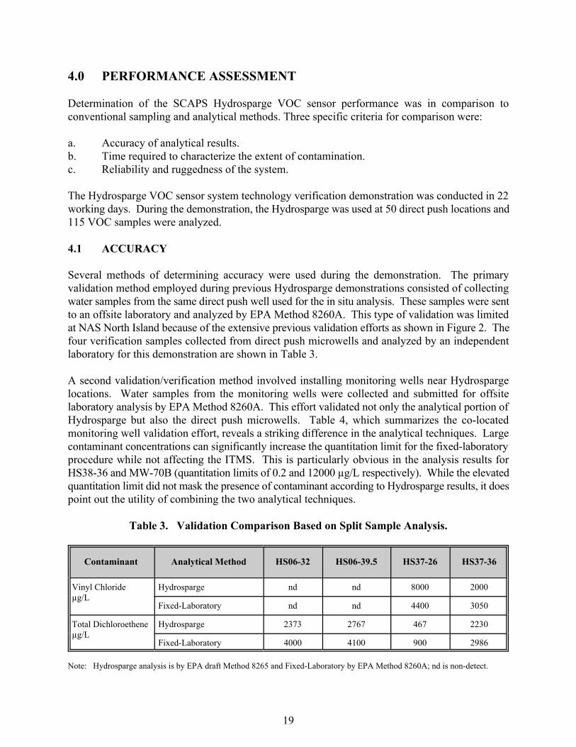
Several methods of determining accuracy were used during the demonstration. The primaryvalidation method employed during previous Hydrosparge demonstrations consisted of collectingwater samples from the same direct push well used for the in situ analysis. These samples were sentto an offsite laboratory and analyzed by EPA Method 8260A. This type of validation was limitedat NAS North Island because of the extensive previous validation efforts as shown in Figure 2. Thefour verification samples collected from direct push microwells and analyzed by an independentlaboratory for this demonstration are shown in Table 3.
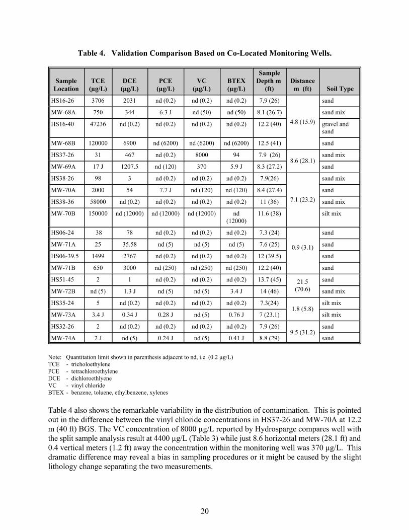
A second validation/verification method involved installing monitoring wells near Hydrospargelocations. Water samples from the monitoring wells were collected and submitted for offsitelaboratory analysis by EPA Method 8260A. This effort validated not only the analytical portion ofHydrosparge but also the direct push microwells. Table 4, which summarizes the co-locatedmonitoring well validation effort, reveals a striking difference in the analytical techniques. Largecontaminant concentrations can significantly increase the quantitation limit for the fixed-laboratoryprocedure while not affecting the ITMS. This is particularly obvious in the analysis results forHS38-36 and MW-70B (quantitation limits of 0.2 and 12000 µg/L respectively). While the elevatedquantitation limit did not mask the presence of contaminant according to Hydrosparge results, it doespoint out the utility of combining the two analytical techniques.
Table 3. Validation Comparison Based on Split Sample Analysis.
Contaminant Analytical Method HS06-32 HS06-39.5 HS37-26 HS37-36
Vinyl Chloride Hydrosparge nd nd 8000 2000µg/L
Fixed-Laboratory nd nd 4400 3050
Total Dichloroethene Hydrosparge 2373 2767 467 2230µg/L
Fixed-Laboratory 4000 4100 900 2986
Note: Hydrosparge analysis is by EPA draft Method 8265 and Fixed-Laboratory by EPA Method 8260A; nd is non-detect.
20
Table 4. Validation Comparison Based on Co-Located Monitoring Wells.
Sample TCE DCE PCE VC BTEX Depth m DistanceLocation (µg/L) (µg/L) (µg/L) (µg/L) (µg/L) (ft) m (ft) Soil Type
Sample
HS16-26 3706 2031 nd (0.2) nd (0.2) nd (0.2) 7.9 (26) sand
4.8 (15.9)MW-68A 750 344 6.3 J nd (50) nd (50) 8.1 (26.7) sand mix
HS16-40 47236 nd (0.2) nd (0.2) nd (0.2) nd (0.2) 12.2 (40) gravel andsand
MW-68B 120000 6900 nd (6200) nd (6200) nd (6200) 12.5 (41) sand
HS37-26 31 467 nd (0.2) 8000 94 7.9 (26) sand mix8.6 (28.1)
MW-69A 17 J 1207.5 nd (120) 370 5.9 J 8.3 (27.2) sand
HS38-26 98 3 nd (0.2) nd (0.2) nd (0.2) 7.9(26) sand mix
7.1 (23.2)MW-70A 2000 54 7.7 J nd (120) nd (120) 8.4 (27.4) sand
HS38-36 58000 nd (0.2) nd (0.2) nd (0.2) nd (0.2) 11 (36) sand mix
MW-70B 150000 nd (12000) nd (12000) nd (12000) nd 11.6 (38) silt mix(12000)
HS06-24 38 78 nd (0.2) nd (0.2) nd (0.2) 7.3 (24) sand
0.9 (3.1)MW-71A 25 35.58 nd (5) nd (5) nd (5) 7.6 (25) sand
HS06-39.5 1499 2767 nd (0.2) nd (0.2) nd (0.2) 12 (39.5) sand
MW-71B 650 3000 nd (250) nd (250) nd (250) 12.2 (40) sand
HS51-45 2 1 nd (0.2) nd (0.2) nd (0.2) 13.7 (45) sand21.5(70.6)MW-72B nd (5) 1.3 J nd (5) nd (5) 3.4 J 14 (46) sand mix
HS35-24 5 nd (0.2) nd (0.2) nd (0.2) nd (0.2) 7.3(24) silt mix1.8 (5.8)
MW-73A 3.4 J 0.34 J 0.28 J nd (5) 0.76 J 7 (23.1) silt mix
HS32-26 2 nd (0.2) nd (0.2) nd (0.2) nd (0.2) 7.9 (26) sand9.5 (31.2)
MW-74A 2 J nd (5) 0.24 J nd (5) 0.41 J 8.8 (29) sand
Note: Quantitation limit shown in parenthesis adjacent to nd, i.e. (0.2 µg/L)TCE - tricholoethylenePCE - tetrachloroethyleneDCE - dichloroethlyeneVC - vinyl chlorideBTEX - benzene, toluene, ethylbenzene, xylenes
Table 4 also shows the remarkable variability in the distribution of contamination. This is pointedout in the difference between the vinyl chloride concentrations in HS37-26 and MW-70A at 12.2m (40 ft) BGS. The VC concentration of 8000 µg/L reported by Hydrosparge compares well withthe split sample analysis result at 4400 µg/L (Table 3) while just 8.6 horizontal meters (28.1 ft) and0.4 vertical meters (1.2 ft) away the concentration within the monitoring well was 370 µg/L. Thisdramatic difference may reveal a bias in sampling procedures or it might be caused by the slightlithology change separating the two measurements.
21
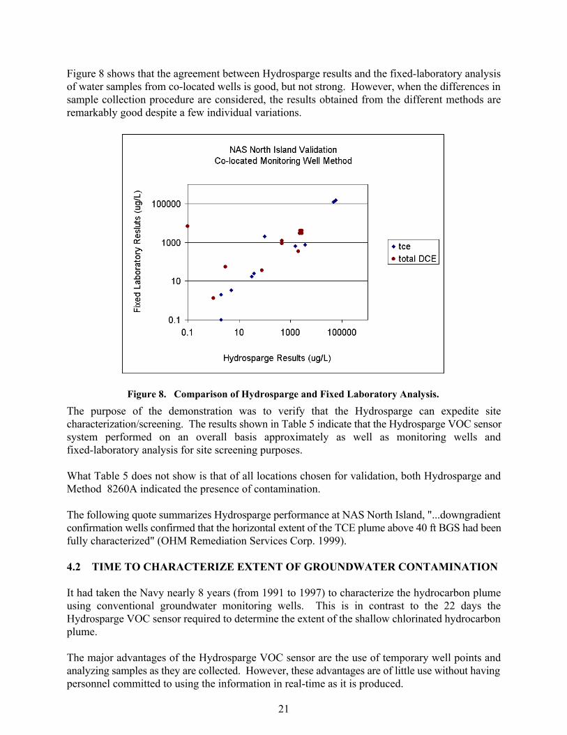
Figure 8. Comparison of Hydrosparge and Fixed Laboratory Analysis.
Figure 8 shows that the agreement between Hydrosparge results and the fixed-laboratory analysisof water samples from co-located wells is good, but not strong. However, when the differences insample collection procedure are considered, the results obtained from the different methods areremarkably good despite a few individual variations.
The purpose of the demonstration was to verify that the Hydrosparge can expedite sitecharacterization/screening. The results shown in Table 5 indicate that the Hydrosparge VOC sensorsystem performed on an overall basis approximately as well as monitoring wells andfixed-laboratory analysis for site screening purposes.
What Table 5 does not show is that of all locations chosen for validation, both Hydrosparge andMethod 8260A indicated the presence of contamination.
The following quote summarizes Hydrosparge performance at NAS North Island, "...downgradientconfirmation wells confirmed that the horizontal extent of the TCE plume above 40 ft BGS had beenfully characterized" (OHM Remediation Services Corp. 1999).
4.2 TIME TO CHARACTERIZE EXTENT OF GROUNDWATER CONTAMINATION
It had taken the Navy nearly 8 years (from 1991 to 1997) to characterize the hydrocarbon plumeusing conventional groundwater monitoring wells. This is in contrast to the 22 days theHydrosparge VOC sensor required to determine the extent of the shallow chlorinated hydrocarbonplume.
The major advantages of the Hydrosparge VOC sensor are the use of temporary well points andanalyzing samples as they are collected. However, these advantages are of little use without havingpersonnel committed to using the information in real-time as it is produced.
22
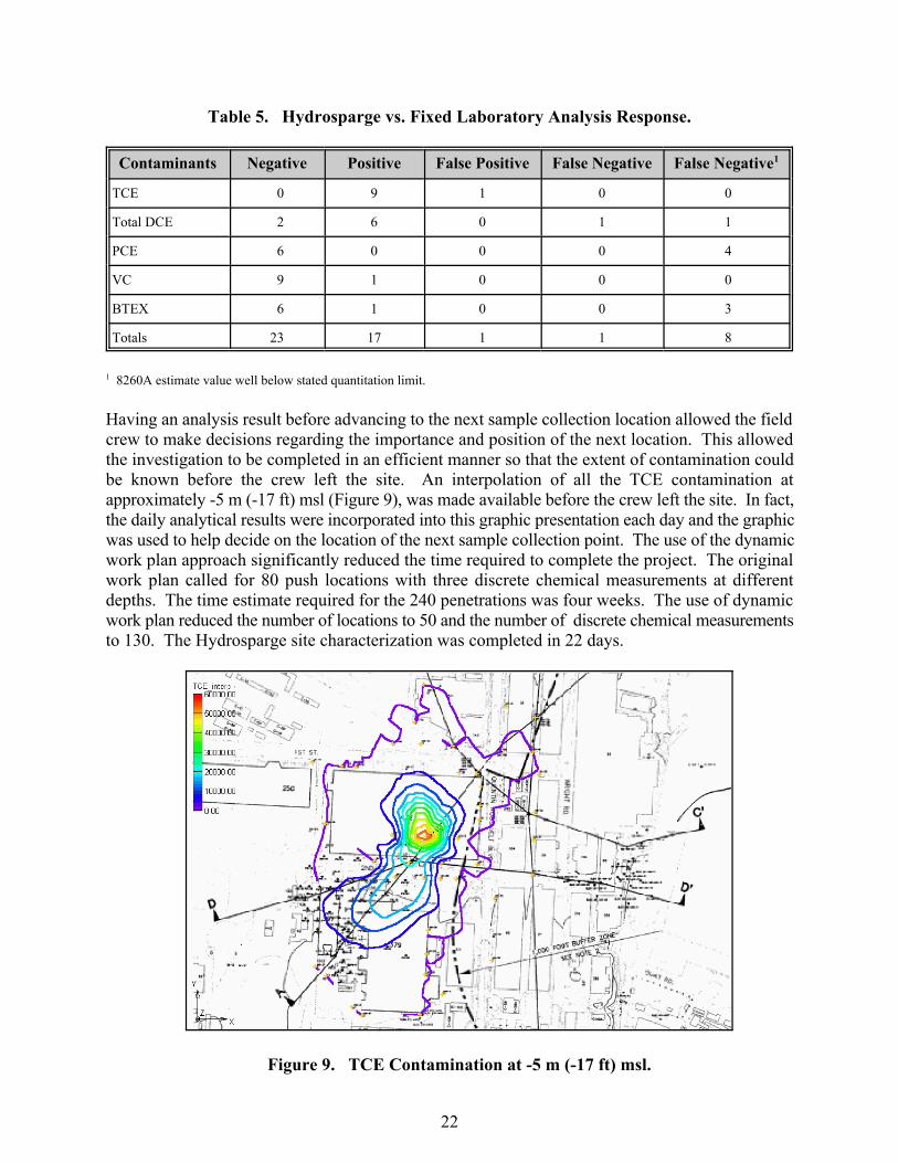
Figure 9. TCE Contamination at -5 m (-17 ft) msl.
Table 5. Hydrosparge vs. Fixed Laboratory Analysis Response.
Contaminants Negative Positive False Positive False Negative False Negative 1
TCE 0 9 1 0 0
Total DCE 2 6 0 1 1
PCE 6 0 0 0 4
VC 9 1 0 0 0
BTEX 6 1 0 0 3
Totals 23 17 1 1 8
8260A estimate value well below stated quantitation limit.1
Having an analysis result before advancing to the next sample collection location allowed the fieldcrew to make decisions regarding the importance and position of the next location. This allowedthe investigation to be completed in an efficient manner so that the extent of contamination couldbe known before the crew left the site. An interpolation of all the TCE contamination atapproximately -5 m (-17 ft) msl (Figure 9), was made available before the crew left the site. In fact,the daily analytical results were incorporated into this graphic presentation each day and the graphicwas used to help decide on the location of the next sample collection point. The use of the dynamicwork plan approach significantly reduced the time required to complete the project. The originalwork plan called for 80 push locations with three discrete chemical measurements at differentdepths. The time estimate required for the 240 penetrations was four weeks. The use of dynamicwork plan reduced the number of locations to 50 and the number of discrete chemical measurementsto 130. The Hydrosparge site characterization was completed in 22 days.
23
4.3 RELIABILITY AND RUGGEDNESS
There were no production delays caused by the ITMS or transfer lines. The only delays were causedby logistical constraints - clearance for the next sample location, striking an unmarked waterline,etc. One of the major requirements for the Hydrosparge VOC sensor to work properly was to havefacility personnel ready to accommodate changes as the work proceeded. Since Hydrosparge ITMSresults were available as samples were collected, onsite real-time decisions to modify the test planwere made to increase the efficiency and cost-effectiveness of the site characterization plan.

This page left blank intentionally.
25
5.0 COST ASSESSMENT
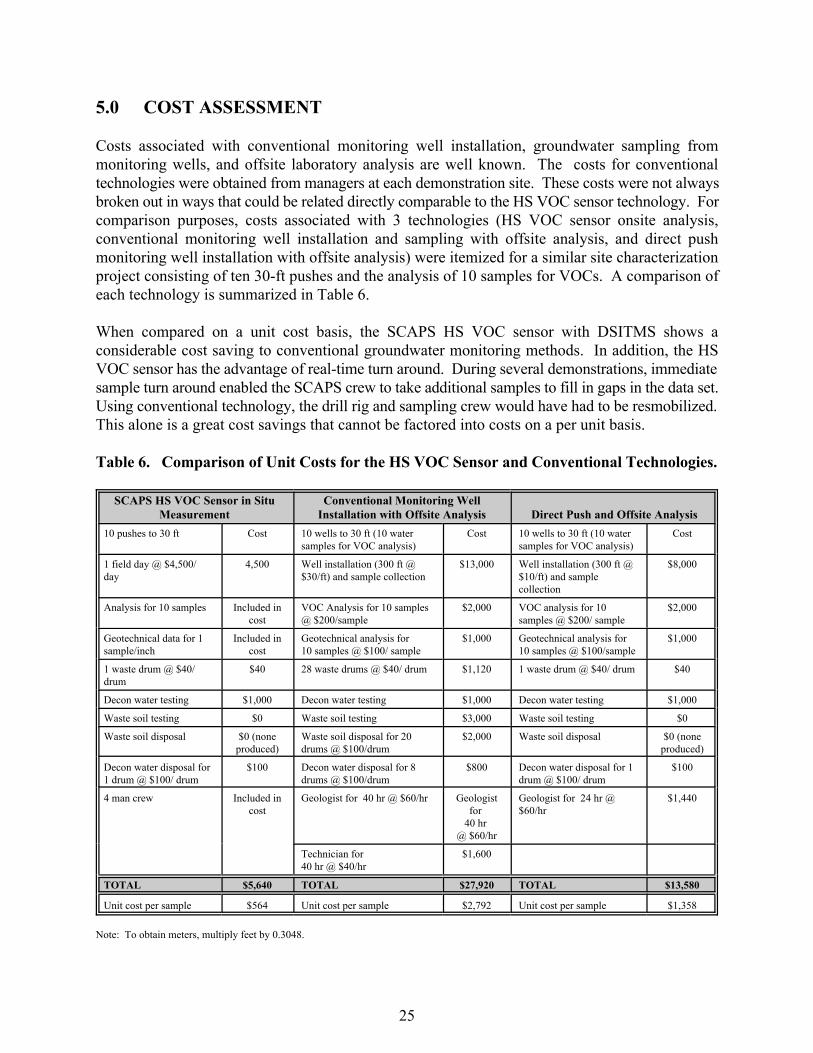
Costs associated with conventional monitoring well installation, groundwater sampling frommonitoring wells, and offsite laboratory analysis are well known. The costs for conventionaltechnologies were obtained from managers at each demonstration site. These costs were not alwaysbroken out in ways that could be related directly comparable to the HS VOC sensor technology. Forcomparison purposes, costs associated with 3 technologies (HS VOC sensor onsite analysis,conventional monitoring well installation and sampling with offsite analysis, and direct pushmonitoring well installation with offsite analysis) were itemized for a similar site characterizationproject consisting of ten 30-ft pushes and the analysis of 10 samples for VOCs. A comparison ofeach technology is summarized in Table 6.
When compared on a unit cost basis, the SCAPS HS VOC sensor with DSITMS shows aconsiderable cost saving to conventional groundwater monitoring methods. In addition, the HSVOC sensor has the advantage of real-time turn around. During several demonstrations, immediatesample turn around enabled the SCAPS crew to take additional samples to fill in gaps in the data set.Using conventional technology, the drill rig and sampling crew would have had to be resmobilized.This alone is a great cost savings that cannot be factored into costs on a per unit basis.
Table 6. Comparison of Unit Costs for the HS VOC Sensor and Conventional Technologies.
SCAPS HS VOC Sensor in Situ Conventional Monitoring WellMeasurement Installation with Offsite Analysis Direct Push and Offsite Analysis
10 pushes to 30 ft Cost 10 wells to 30 ft (10 water Cost 10 wells to 30 ft (10 water Costsamples for VOC analysis) samples for VOC analysis)
1 field day @ $4,500/ 4,500 Well installation (300 ft @ $13,000 Well installation (300 ft @ $8,000day $30/ft) and sample collection $10/ft) and sample
collection
Analysis for 10 samples Included in VOC Analysis for 10 samples $2,000 VOC analysis for 10 $2,000cost @ $200/sample samples @ $200/ sample
Geotechnical data for 1 Included in Geotechnical analysis for $1,000 Geotechnical analysis for $1,000sample/inch cost 10 samples @ $100/ sample 10 samples @ $100/sample
1 waste drum @ $40/ $40 28 waste drums @ $40/ drum $1,120 1 waste drum @ $40/ drum $40drum
Decon water testing $1,000 Decon water testing $1,000 Decon water testing $1,000
Waste soil testing $0 Waste soil testing $3,000 Waste soil testing $0
Waste soil disposal $0 (none Waste soil disposal for 20 $2,000 Waste soil disposal $0 (noneproduced) drums @ $100/drum produced)
Decon water disposal for $100 Decon water disposal for 8 $800 Decon water disposal for 1 $1001 drum @ $100/ drum drums @ $100/drum drum @ $100/ drum
4 man crew Included in Geologist for 40 hr @ $60/hr Geologist Geologist for 24 hr @ $1,440cost for $60/hr
40 hr @ $60/hr
Technician for $1,60040 hr @ $40/hr
TOTAL $5,640 TOTAL $27,920 TOTAL $13,580
Unit cost per sample $564 Unit cost per sample $2,792 Unit cost per sample $1,358
Note: To obtain meters, multiply feet by 0.3048.

This page left blank intentionally.
27
6.0 REFERENCES
1. American Society for Testing and Material (ASTM). (1991). “Method D-3441, Standardpractice for geophysical cone penetrometry,” ASTM 04.08 (D-3441), West Conshohocken,PA.
2. Davis, W. M., Wise, M. B, Furey, J. S. and Thompson, C. V. (1998a). “Rapid detection ofvolatile organic compounds in groundwater by in situ purge and direct sampling ion trapmass spectrometry,” Field Analytical Chemistry and Technology 2, 86-96.
3. Davis, W. M., Furey, J. S. and Porter, B. (1998b). “Field screening of VOCs in groundwater using the hydrosparge VOC sensor,” Current Protocols in Field Analytical Chemistry,V. Lopez-Avila, ed., J. Wiley and Sons, Inc., New York, NY.
4. Geosciences. (1993). “Final site assessment report environmental soil and groundwaterinvestigation, Naval Aviation Depot, Naval Air Station, North Island, San Diego,California.”
5. Jacobs Engineering. (1991). “NADEP- North Island Coronado, California Site Assessment,Final Report.”
6. Lee, L. T., Davis, W. M., Goodson, R. A., Powell, J. F., and Register, B. A. (1994). “Sitecharacterization and analysis penetrometer system (SCAPS) field investigation at the SierraArmy Depot, California,” Technical Report GL-94-4, U.S. Army Engineer WaterwaysExperiment Station, Vicksburg, MS.
7. OHM Remediation Services Corp. (1997) “Free product recovery site buildings 379 and397, Naval Aviation Depot, Naval Air Station North Island, Coronado, California.”
8. U.S. Environmental Protection Agency. (1993) “Test methods for evaluating solid waste;physical/chemical methods, SW-846 Third Edition,” Washington, DC.
9. U.S. Environmental Protection Agency. (1994). “Test methods for evaluating solid waste;physical/chemical methods, SW-846,” Draft Method 8265: Volatiles in Water, Soil, and Airby Direct Sampling Ion Trap Mass Spectrometry. Washington, DC.
10. Wise, M. B., and Guerin, M. R. (1997). “Direct sampling MS for environmental screening,”Analytical Chemistry 69, 26A-32A.
11. Wise, M. B., Thompson, C. V., Merriweather, R, and Guerin, M. R. (1997). “Review ofdirect MS analysis of environmental samples,” Field Analytical Chemistry and Technology1(5), 251-276.

This page left blank intentionally.
A-1
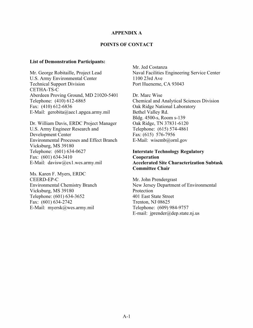
APPENDIX A
POINTS OF CONTACT
List of Demonstration Participants:
Mr. George Robitaille, Project Lead Naval Facilities Engineering Service CenterU.S. Army Environmental Center 1100 23rd AveTechnical Support Division Port Hueneme, CA 93043CETHA-TS-CAberdeen Proving Ground, MD 21020-5401 Dr. Marc WiseTelephone: (410) 612-6865 Chemical and Analytical Sciences DivisionFax: (410) 612-6836 Oak Ridge National LaboratoryE-Mail: [email protected] Bethel Valley Rd.
Dr. William Davis, ERDC Project Manager Oak Ridge, TN 37831-6120U.S. Army Engineer Research and Telephone: (615) 574-4861Development Center Fax: (615) 576-7956Environmental Processes and Effect Branch E-Mail: [email protected], MS 39180Telephone: (601) 634-0627Fax: (601) 634-3410E-Mail: [email protected]
Ms. Karen F. Myers, ERDC CEERD-EP-C Mr. John PrendergrastEnvironmental Chemistry Branch New Jersey Department of Environmental Vicksburg, MS 39180 ProtectionTelephone: (601) 634-3652 401 East State StreetFax: (601) 634-2742 Trenton, NJ 08625E-Mail: [email protected] Telephone: (609) 984-9757
Mr. Jed Costanza
Bldg. 4500-s, Room s-139
Interstate Technology RegulatoryCooperation Accelerated Site Characterization SubtaskCommittee Chair
E-mail: [email protected]

ESTCP Program Office
901 North Stuart StreetSuite 303Arlington, Virginia 22203
(703) 696-2117 (Phone)(703) 696-2114 (Fax)
e-mail: [email protected]

ESTCP Program Office
901 North Stuart StreetSuite 303Arlington, Virginia 22203
(703) 696-2117 (Phone)(703) 696-2114 (Fax)
e-mail: [email protected]