estcp cost and performance report cost and performance report ... (e.g., surface towed ordnance...

ESTCPCost and Performance Report

ENVIRONMENTAL SECURITYTECHNOLOGY CERTIFICATION PROGRAM

U.S. Department of Defense

(MM-0605)

Commercial-Off-The-Shelf Vehicles for Towed Array Magnetometry

September 2009

i

COST & PERFORMANCE REPORT Project: MM-0605

TABLE OF CONTENTS

Page

1.0 EXECUTIVE SUMMARY ....................................................................... 1

2.0 INTRODUCTION.................................................................................. 3 2.1 BACKGROUND........................................................................... 3 2.2 OBJECTIVES OF THE DEMONSTRATION ....................................... 4 2.3 REGULATORY DRIVERS.............................................................. 5

3.0 TECHNOLOGY.................................................................................... 7 3.1 TECHNOLOGY DESCRIPTION ...................................................... 7

3.1.1 Overview........................................................................... 7 3.1.2 Theory of Operation.............................................................. 7 3.1.3 Schematics and Layout..........................................................10 3.1.4 Chronological Summary ........................................................11 3.1.5 Summary of Development......................................................11

3.2 ADVANTAGES AND LIMITATIONS OF THE TECHNOLOGY .............11

4.0 PERFORMANCE OBJECTIVES...............................................................15

5.0 SITE DESCRIPTION.............................................................................17 5.1 SITE LOCATION AND HISTORY...................................................17 5.2 SITE GEOLOGY.........................................................................17 5.3 MUNITIONS CONTAMINATION ...................................................17

6.0 TEST DESIGN ....................................................................................19 6.1 CONCEPTUAL EXPERIMENTAL DESIGN ......................................19 6.2 SITE PREPARATION...................................................................19 6.3 SYSTEM SPECIFICATION............................................................19

6.3.1 Operating Parameters for the Technology ...................................20 6.4 DATA COLLECTION ..................................................................20

6.4.1 Scale ...............................................................................20 6.4.2 Sample Density...................................................................20 6.4.3 Quality Checks ...................................................................21 6.4.4 Data Summary ...................................................................21

6.5 VALIDATION............................................................................21

7.0 DATA ANALYSIS AND PRODUCTS .......................................................23 7.1 PREPROCESSING.......................................................................23 7.2 TARGET SELECTION FOR DETECTION.........................................24 7.3 PARAMETER ESTIMATES...........................................................24

TABLE OF CONTENTS (continued)

Page

ii

7.4 CLASSIFIER AND TRAINING.......................................................24 7.5 DATA PRODUCTS......................................................................24

8.0 PERFORMANCE ASSESSMENT .............................................................25 8.1 SUMMARY ...............................................................................25 8.2 PERFORMANCE CRITERIA .........................................................25 8.3 PERFORMANCE CONFIRMATION METHODS.................................25 8.4 DATA ANALYSIS, INTERPRETATION AND EVALUATION...............26

8.4.1 Bulk Vehicle SignatureCOctant Tests ........................................26 8.4.2 Bulk Vehicle SignatureCGeophysical Survey of Legacy Area ...........30 8.4.3 Bulk Signature Summary .......................................................48 8.4.4 Effect of De-Median Filter Window Length ................................49 8.4.5 Effect of Rough Terrain ........................................................52 8.4.6 Vehicle Ride ......................................................................55 8.4.7 Vehicle Terrain Handling Capability .........................................55 8.4.8 Conclusions .......................................................................55

9.0 COST ASSESSMENT ............................................................................57 9.1 COST MODEL ...........................................................................57 9.2 COST DRIVERS .........................................................................58 9.3 COST BENEFIT..........................................................................58

10.0 IMPLEMENTATION ISSUES..................................................................59 10.1 ENVIRONMENTAL AND REGULATORY ISSUES.............................59 10.2 END-USER ISSUES .....................................................................59 10.3 RELEVANT PROCUREMENT ISSUES ............................................59 10.4 AVAILABILITY OF THE TECHNOLOGY ........................................59 10.5 SPECIALIZED SKILLS AND TRAINING..........................................59

11.0 REFERENCES.....................................................................................61 APPENDIX A POINTS OF CONTACT......................................................................... A-1

iii

LIST OF FIGURES

Page Figure 1. Conceptual illustration depicting how survey direction affects magnetic

signature.................................................................................................................. 8 Figure 2. Sample unfiltered and filtered data taken with one of several UTVs tested

at the Devens Test Site, clearly showing the heading-dependent effect of vehicle signature. .................................................................................................... 9

Figure 3. Data taken with steel John Deere Gator tow vehicle showing “cloudy” artifacts due to pitch and roll over rough terrain................................................... 10

Figure 4. Club Car 1550XRT towing the VSEMS platform................................................ 10 Figure 5. Octant Test, Mag 15 ft behind vehicle, skidplate removed .................................. 28 Figure 6. Octant Test, Mag 15 ft behind vehicle, skidplate installed................................... 28 Figure 7. Octant Test, Mag 17 ft behind vehicle, skidplate removed .................................. 29 Figure 8. Octant Test, Mag 17 ft behind vehicle, skidplate installed................................... 29 Figure 9. APG site surveyed in 2006 with Chenowth buggy, mags 15 ft back,

uncorrected............................................................................................................ 32 Figure 10. APG site legacy area section surveyed in 2006 with Chenowth buggy, mags

15 ft back, uncorrected.......................................................................................... 33 Figure 11. APG site legacy area section surveyed in 2006 with Chenowth buggy, mags

15 ft back, with bidirectional correction ............................................................... 35 Figure 12. APG site legacy area plus adjacent section surveyed in 2006 with Chenowth

buggy, mags 15 ft back, with bidirectional correction.......................................... 36 Figure 13. APG site legacy area plus adjacent section surveyed in 2006 with Chenowth

buggy, mags 15 ft back, with de-median correction............................................. 37 Figure 14. Legacy area surveyed with COTS vehicle, mags 15 ft back, skidplate

attached, uncorrected ............................................................................................ 39 Figure 15. Legacy area surveyed with COTS vehicle, mags 15 ft back, skidplate

attached, with bidirectional correction.................................................................. 41 Figure 16. Legacy area surveyed with COTS vehicle, mags 15 ft back, skidplate

installed, with de-median filter correction ............................................................ 43 Figure 17. Legacy area surveyed with COTS Vehicle, mags 17 ft back, skidplate

removed, uncorrected............................................................................................ 44 Figure 18. Legacy area surveyed with COTS vehicle, mags 17 ft back, skidplate

removed, with bidirectional correction ................................................................. 46 Figure 19. Legacy area surveyed with COTS vehicle, mags 17 ft back, skidplate

removed, with de-median filter correction............................................................ 48 Figure 20. Nine objects, anomaly peak amplitude as a function of median filter

window length....................................................................................................... 50 Figure 21. Nine objects, anomaly full width at half max as a function of median filter

window length....................................................................................................... 51 Figure 22. Legacy area with rough areas shown as black lines, color scale pushed to

show washboard pattern........................................................................................ 53 Figure 23. Blowup to show washboard pattern...................................................................... 54

iv

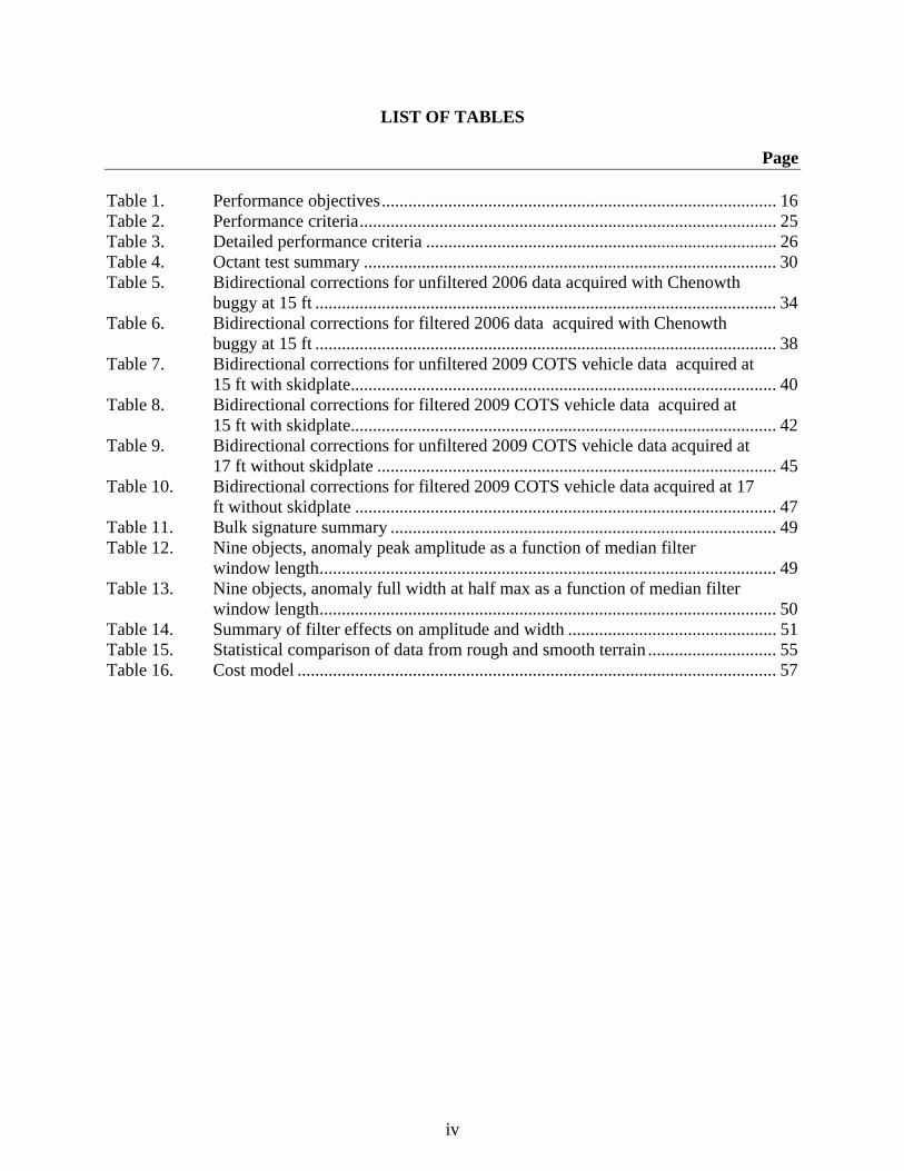
LIST OF TABLES

Page Table 1. Performance objectives......................................................................................... 16 Table 2. Performance criteria.............................................................................................. 25 Table 3. Detailed performance criteria ............................................................................... 26 Table 4. Octant test summary ............................................................................................. 30 Table 5. Bidirectional corrections for unfiltered 2006 data acquired with Chenowth

buggy at 15 ft ........................................................................................................ 34 Table 6. Bidirectional corrections for filtered 2006 data acquired with Chenowth

buggy at 15 ft ........................................................................................................ 38 Table 7. Bidirectional corrections for unfiltered 2009 COTS vehicle data acquired at

15 ft with skidplate................................................................................................ 40 Table 8. Bidirectional corrections for filtered 2009 COTS vehicle data acquired at

15 ft with skidplate................................................................................................ 42 Table 9. Bidirectional corrections for unfiltered 2009 COTS vehicle data acquired at

17 ft without skidplate .......................................................................................... 45 Table 10. Bidirectional corrections for filtered 2009 COTS vehicle data acquired at 17

ft without skidplate ............................................................................................... 47 Table 11. Bulk signature summary ....................................................................................... 49 Table 12. Nine objects, anomaly peak amplitude as a function of median filter

window length....................................................................................................... 49 Table 13. Nine objects, anomaly full width at half max as a function of median filter

window length....................................................................................................... 50 Table 14. Summary of filter effects on amplitude and width ............................................... 51 Table 15. Statistical comparison of data from rough and smooth terrain ............................. 55 Table 16. Cost model ............................................................................................................ 57

v

ACRONYMS AND ABBREVIATIONS APG Aberdeen Proving Grounds ATV all-terrain vehicle COTS commercial off-the-shelf DGM digital geophysical mapping EM electromagnetic EMI electromagnetic induction ESTCP Environmental Security Technology Certification Program GPS Global Positioning System MEC munitions and explosives of concern MTADS Multi-Sensor Towed Array Detection System nT nanotesla PI principal investigator PPS pulse per second RF radio frequency RTK real-time kinematic SAIC Science Applications International Corporation STOLS Surface Towed Ordnance Location System UTV utility vehicle UXO unexploded ordnance VSEMS vehicular simultaneous EMI and magnetometer system YPG Yuma Proving Grounds

This page left blank intentionally.

Technical material contained in this report has been approved for public release.

vii

ACKNOWLEDGEMENTS The author wishes to thank the Environmental Security Technology Certification Program (ESTCP) Program Office for funding this project.

1

1.0 EXECUTIVE SUMMARY

Vehicular-towed magnetometer arrays have been used for munitions and explosives of concern (MEC) detection since the late 1980s. However, most vehicles are highly ferromagnetic due to their ferrous frame, skin, and drive train, and the resulting magnetic self-signature can easily overwhelm the signal from subsurface objects and render the data useless. Further, because the vehicle signature is induced by the Earth’s magnetic field, it is not constant; it changes primarily with the vehicle’s orientation relative to north, and secondarily with the vehicle’s pitch and roll. Several successful vehicle-towed magnetometer arrays have addressed the vehicle signature problem through the use of custom-built nonferrous, aluminum-framed vehicles that minimize vehicle self-signature. However, the cost of these vehicles was in excess of $100,000, putting them out of range of commercial unexploded ordnance (UXO) contractors. The logical question is: Is this kind of expensive custom vehicle absolutely necessary to acquire high-quality towed array magnetometer data, or can a contractor employ a vehicle with a higher signature and filter out its effects? Under this project we tested a number of commercial off-the-shelf (COTS) side-by-side utility vehicles (UTV) and an all-terrain vehicle (ATV) for their applicability as tow vehicles for a towed magnetometer array by measuring their magnetic signature and determining if the signature can be removed through simple filtering techniques to yield data of a similar quality to data obtained using a custom-built vehicle. Science Applications International Corporation (SAIC) selected what it felt was the best compromise of low signature, cargo space, terrain-handling capability, and rideCthe aluminum-framed Club Car XRT 1550Cpurchased it, and adapted it to pull SAIC’s full-sized vehicular simultaneous electromagnetic induction (EMI) and magnetometer system (VSEMS) mag/electromagnectic (EM) 61 towed platform (developed under ESTCP project MM-0208). We found that this vehicle engenders only a moderate signature in the data and that this signature can be easily removed with the de-median filter in Geosoft Oasis Montaj that is already commonly employed for filtering geophysical data.

3

2.0 INTRODUCTION

2.1 BACKGROUND

Total field magnetometers are proven instruments for MEC detection. Their high sensitivity makes them particularly appropriate for detecting major caliber air-dropped munitions like 250- lb bombs that are large and ferrous, and can penetrate deep. To maximize the number of survey acres per day, a wide swath may be obtained by ganging total field magnetometers together in an array. Because of the weight of the required batteries and electronics, the wear and tear on the person carrying the equipment, and the desire to increase survey speed, it is natural to want to tow such a magnetometer array behind a vehicle. However, the magnetometer’s very sensitivity makes this difficult. Most vehicles are highly ferromagnetic due to their ferrous frame, skin, and drive train, and a towing vehicle’s magnetic self-signature can overwhelm the signal from subsurface objects and render the data useless. Further, because the vehicle signature is induced by the Earth’s magnetic field, it is not constant; it changes primarily with the vehicle’s orientation relative to north, and secondarily with the vehicle’s pitch and roll. Historically, successful vehicle-towed magnetometer arrays (e.g., Surface Towed Ordnance Location System [STOLS], Multi-Sensor Towed Array Detection System [MTADS], and VSEMS) have addressed the vehicle signature problem using vehicles custom-built out of nonferrous materials to minimize vehicle self-signature. Both MTADS and VSEMS utilize dune buggies custom-built by Chenowth Racing with an aluminum frame and a magnesium alloy engine. Fifteen years ago, the cost of these vehicles was in excess of $100,000, putting them out of range of most commercial UXO contractors. The logical question is: Is this kind of vehicle absolutely necessary to acquire high-quality towed array magnetometer data, or can a system employ a vehicle with a higher signature and filter out its effects? Since the development of MTADS and VSEMS, a variety of COTS ATVs and so-called “side-by-side” UTVs have become available. An ATV is a small vehicle that is straddled like a motorcycle and has handlebars and hand controls like a motorcycle, whereas a side-by-side UTV looks like a cross between a golf cart and a small Jeep, typically has a small dump bed on the back, upright seating for two adults, the seats oriented side-by-side, and a steering wheel, and brake and accelerator pedals like a car. By way of example, a ubiquitous side-by-side UTV is the John Deere Gator. The objective of this project was to test a number of these COTS vehicles for their applicability as tow vehicles for a towed magnetometer array by measuring their magnetic signature and seeing if non-zero vehicle signature can be removed through simple filtering techniques to yield data of a similar quality to data obtained using a custom-built vehicle. A small towed platform was designed and constructed that allowed two magnetometers, two EM61s, and a Global Positioning System (GPS) to be easily slid along a fiberglass backbone to vary the vehicle-to-sensor separation. Ten vehicles were tested, ranging in size from a small ATV up through a Jeep Wrangler, but the project’s emphasis was on side-by-side UTVs since these have roll cages, shade, ample space for electronics, and the opportunity for weather-tight enclosure, whereas small ATVs have none of these things. Six UTVs were tested using the adjustable platform. A full description of these vehicles and the data generated is contained in “MM-0605 Vehicle Signature Report and Geophysical Procedures for Vehicle Signature Measurement” submitted to the ESTCP Program Office in April 2007. SAIC selected what it felt was the best compromise of low signature, cargo space,

4

terrain-handling capability, and rideCthe aluminum-framed Club Car XRT 1550Cpurchased it with SAIC funds, and adapted it to pull SAIC’s full-sized VSEMS mag/EM61 towed platform (developed under ESTCP project MM-0208). During preliminary testing at the small Devens test site in Massachusetts, we found that this vehicle engenders only a moderate signature in the data and that this signature can be easily removed with the de-median filter already used by both MTADS and VSEMS. As per the project plan, we demonstrated this vehicle, towing the full-sized VSEMS platform, at Aberdeen Proving Grounds (APG), MD, to measure its magnetic signature and evaluate its performance on a near-real-world site with a greater variety of terrain than the small site at Devens.

2.2 OBJECTIVES OF THE DEMONSTRATION

The objectives of the demonstration were:

To acquire survey data with the new COTS vehicle over a site that has realistic terrain roughness and compare these data with data previously acquired over the same site using the VSEMS custom aluminum-framed buggy.

To apply signature removal algorithms to the data and judge whether there is a significant difference in data quality attributable to the COTS vehicle and its higher bulk magnetic signature.

To evaluate whether there are significant effects in signature-induced artifacts caused by vehicle pitch and roll over rough terrain.

To evaluate the COTS vehicle’s terrain-handling capability and ride and compare them to the buggy’s.

In support of these objectives, we:

Deployed to the Standardized UXO Demonstration Test Site at APG

Performed octant tests (placed the system in a clean area and oriented the vehicle and towed platform north, northeast, east, etc.) to get a quick snapshot of vehicle signature in several configurations

Surveyed the calibration test grid and open field legacy area using a conservative configuration (with the sensors as far back on the platform as they can possibly go, and without the steel skidplate) and a more aggressive configuration (with the sensors at their nominal 15ft distance from the vehicle, and with the skidplate)

Examined clean areas in the data to measure bulk vehicle signature and perturbations to that bulk signature caused by vehicle motion on uneven terrain

Varied the time window of the filtering and examined the effect on bulk signature and on signal and amplitude of MEC targets.

5

2.3 REGULATORY DRIVERS

The primary driver is the continued need to develop tools to detect MEC. The documented use of a COTS vehicle to tow a magnetometer array and generate high-quality data will allow more contractors to use towed magnetometer arrays.

7

3.0 TECHNOLOGY

3.1 TECHNOLOGY DESCRIPTION

3.1.1 Overview

A magnetometer’s M/R3 omnidirectional sensitivity (where M is a magnetic moment and R is the distance detector and object) makes it susceptible to the magnetic signature not only of buried MEC but also of a towing vehicle. This signature changes primarily with the vehicle’s changing orientation relative to north and secondarily as the vehicle pitches and rolls about the horizontal plane. For small to moderately sized vehicles, given a reasonable distance between the vehicle and the towed magnetometer array, the vehicle’s signature is small enough and changes slowly and predictably enough with orientation relative to north that the signature can be removed with the same filtering techniques used to remove long-wavelength geology, diurnal drift, and other slowly changing effects. As vehicle size and ferrous content increases, however, small fast changes in vehicle pitch and roll begin to contribute substantially to vehicle signature in a way that defies removal. When this effect begins to dominate, the vehicle is too large and/or the sensors are too close.

3.1.2 Theory of Operation

Any ferrous object in the Earth’s magnetic field has a magnetic moment induced in it. The field produced by that moment adds vectorially to the Earth’s field. The magnitude of this vector sum is measured by a total field magnetometer. During data processing, the magnitude of the Earth’s field is then subtracted off, leaving the anomalous field. From sufficiently far away, even the complex field from a vehicle resembles a point dipole. Grossly speaking, the induced dipole from a vehicle will tend to align north and will tend to have a south-facing positive lobe, and a north-facing negative lobe. This means that, if the vehicle towing a magnetometer array is headed north, the magnetometers will be in the positive lobe of the induced dipole. Conversely, if the vehicle is headed south, the magnetometers will be in the negative lobe of the anomaly created by the induced dipole. This is depicted in the conceptual illustration below. Because of the directional nature of the vehicle’s signature, north-going and south-going traverses are affected by the vehicle differently and contain different vehicle-induced offsets. Because the vehicle is an extended object, not a point dipole and the sensors are in the same plane as the object (not above the object as with detection of a buried object), the “in the negative lobe of the anomaly” explanation is, in fact, a heuristic simplification, and in practice, different vehicles may have the “north positive” and “south negative” rules flipped around. However, the conceptual illustration is extremely useful in that it does help one visualize why the measured vehicle signature changes in passes of opposite direction and how this generates the streaks that one sees in vehicle-towed magnetometer data.

8

Figure 1. Conceptual illustration depicting how survey direction affects magnetic signature.

The image on the left in Figure 2 shows data obtained with a Yamaha Rhino (one of several UTVs tested), with the magnetometers 20 ft behind the vehicle. The area was surveyed in a racetrack-style pattern, with the traverses on the left side of the image obtained in north-going passes and the traverses on the right side of the image obtained in south-going passes. The left side of the image (the north-going passes) is lighterChas a higher average valueCthan the right side of the image (the south-going passes). For this vehicle, at this 20 ft sensor-to-vehicle separation, the difference between north- and south-going traverses is about 40 nanotesla (nT). This value is calculated by defining small areas of interest in each of the north-going and the south-going sides, each containing no other magnetic anomalies, averaging the data in each area, and then subtracting the two averaged values. On most real surveys, a racetrack pattern is not used, and instead, adjacent traverses are usually acquired in opposite directions. In this case, we divide the data into north-going and south-going sets, select a single area of interest that contains some of each set, independently accumulate the average values of north-going and south-going traverses, and subtract them. In either case, we call this value the “bulk signature.” While we often use the terms “bulk signature” and “signature” interchangeably, the “signature” is a vector quantity whose magnitude is different depending on the vehicle’s orientation and the point of measurement, whereas the “bulk signature” is a single number representing, for a fixed vehicle-to-sensor distance, the worst-case difference in sensor readings taken in opposite directions. It is usually clear from the context which is meant. As long as the directionally dependent signature is the only dominant effect, it changes slowly and can be easily filtered out. In the images in Figure 2, the left image is unfiltered, and the right image has had a de-median filter with a 6 sec time window applied to remove the vehicle signature and other long-wavelength effects. Independent analysis by both SAIC and by Dan Steinhurst of Nova Research (the operator of vehicular MTADS) have shown that this sort of de-median filter does a good job at removing slowly changing vehicle effects, along with diurnal drift, long-wavelength geology, and small intersensor offsets that create lines along the direction of travel sometimes informally referred to as “corduroy.”

9

Figure 2. Sample unfiltered (left) and filtered (right) data taken with one of several UTVs

tested (a Yamaha Rhino, mags 20 ft back) at the Devens Test Site, clearly showing the heading-dependent effect of vehicle signature. The image on the left has approximately 40 nT

of bulk signature. The image on the right has had bulk signature removed through de-median filtering. Image scale is ± 50 nT.

The key here is the phrase “slowly changing.” Although the vehicle’s signature varies primarily with yaw (orientation relative to north), it also changes with vehicle roll and pitch. As terrain roughness increases, roll and pitch increase, creating fast-changing perturbations in the data that the de-median filter can’t take out. These artifacts show up as a “clouding” of the data (essentially a disturbance in an otherwise smooth background). An example of “cloudy” data is shown in Figure 3 on the right. Note that both images have been de-median filtered using a 6 sec window, the effect of which has been to remove the azimuthally varying vehicle signature (that is, there is no obvious light/dark bias in either image resulting from the difference in signature north to south), but the image on the right clearly has artifacts that the image on the left does not. These are due to pitch-and-roll-based changes in vehicle signature caused by localized terrain roughness. Short of putting the vehicle on a jig that allows for careful roll and pitch of the entire vehicle and taking a full set of measurements, it is difficult to quantify and predict the effect of pitch and roll. Some sites are simply rougher than others, and for a given vehicle and sensor distance, some sites may engender more of these sort of artifacts than other sites. For example, if one had to survey a very smooth section of beach on an island and was prohibitively expensive to transport a vehicle onto the island and a steel UTV such as a Gator was available on-island, use of such a vehicle might be plausible. But if these artifacts appear in the data at a magnitude that begins to interfere with detection and analysis of the targets of interest, the vehicle signature is too high and the magnetometers are too close.

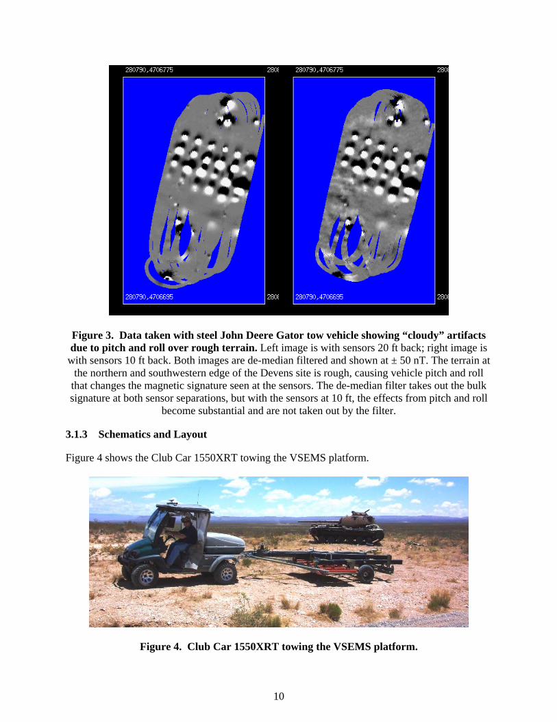
10

Figure 3. Data taken with steel John Deere Gator tow vehicle showing “cloudy” artifacts due to pitch and roll over rough terrain. Left image is with sensors 20 ft back; right image is

with sensors 10 ft back. Both images are de-median filtered and shown at ± 50 nT. The terrain at the northern and southwestern edge of the Devens site is rough, causing vehicle pitch and roll

that changes the magnetic signature seen at the sensors. The de-median filter takes out the bulk signature at both sensor separations, but with the sensors at 10 ft, the effects from pitch and roll

become substantial and are not taken out by the filter.

3.1.3 Schematics and Layout

Figure 4 shows the Club Car 1550XRT towing the VSEMS platform.

Figure 4. Club Car 1550XRT towing the VSEMS platform.

11

3.1.4 Chronological Summary

Fall 2006. A simple two-magnetometer and two-EM61 towed platform was developed to allow vehicle signatures to be evaluated with adjustable vehicle-to-sensor separation. Ten vehicles ranging from an ATV to a Jeep were procured through borrowing or renting, and tested at the Devens, MA, test site over a 4-month period.

Spring 2007. Data was analyzed. Aluminum-framed vehicles (Club Car and Bobcat) were determined to have best signature characteristics of all the UTVs. We verified that a de-median filter did a good job removing the already low vehicle signature. Unfortunately these particular aluminum-framed vehicles do not have fully-independent rear suspension. This resulted in a very stiff ride. We had concerns that the ride was so stiff that it might make the vehicle a poor choice for day-in, day-out digital geophysical mapping (DGM), but the manufacturer told us that the suspension was designed to have 600 lb of load in the dump bed. We felt that once the vehicle was equipped with all the electronics (which includes seven car batteries) the suspension would be sufficiently preloaded.

Fall 2007. Procured demonstrator model of 2007 Club Car for testing (the previous one tested was 2004 model) to be absolutely certain that the vehicle we were about to purchase would have signature similar to the one tested.

Winter 2008. Purchased 2007 Club Car 1550XRT, with enclosure and heat, using SAIC funds.

Spring 2008. Performed final adaptation of Club Car 1550XRT to pull VSEMS trailer. This involved removing the dump bed, mounting all VSEMS electronics in a clamshell on the back deck, outfitting with alloy wheels, demagnetizing tire beads, and adapting the trailer hitch for the disparate vehicle/platform height. Performed preliminary testing of vehicle at Devens test site. Preloading the suspension from the weight of the seven car batteries made the ride quality of the fully-loaded vehicle acceptable.

Summer 2009. Final demonstration at APG.

3.1.5 Summary of Development

A market survey was performed to identify vehicles within the ATV and UTV classes. Representative vehicles were procured and tested, with an emphasis on UTVs. Their bulk magnetic signature was measured at distances of 5 ft, 10 ft, 15 ft, and 20 ft, and filtering techniques were used to try to remove the signature. One UTV was identified as having an aluminum frame, and thus had a substantially lower magnetic signature than the others. This vehicle was procured, adapted to tow the VSEMS array, and tested at APG.

3.2 ADVANTAGES AND LIMITATIONS OF THE TECHNOLOGY

Towed array magnetometry is most directly applicable to large, vehicularly hospitable sites that contain major caliber air-dropped munitions (e.g., 250 lb bombs) and do not have geology with iron-bearing soil. If munitions of interest are between 60 mm and 155 mm, published reports indicate that magnetometers and EM61s have a similar performance envelope. For munitions

12

smaller than 60 mm with little ferrous content, published reports indicate that the performance advantage tips toward the EM61. As terrain becomes more rugged and less hospitable to vehicular surveys vehicle-towed arrays themselves become less applicable, regardless of the choice of sensor. The alternative technology to a COTS vehicle is development of a custom low-ferrous vehicle with an aluminum frame. Because of the high (greater than $100,000) cost, only three of these vehicles are in existence, all built by Chenowth Racing. These vehicles, sometimes incorrectly referred to as “dune buggies” (they are not; they are off-road racing vehicles), have worked well (the MTADS vehicle is still in use, and the STOLS/VSEMS vehicle was retired only recently), but unlike a COTS UTV, they do not have four-wheel drive. They are difficult to make weatherproof (unlike a COTS vehicle with an enclosure). Further, even the custom $100,000 aluminum-framed dune buggies have ferrous components (the internal engine and transaxle components, for example, are steel), and because, for practical reasons, you can’t tow sensors infinitely far back, even these vehicles have a non-zero bulk magnetic signature at practical towing distances of 15 or 20 ft. Although signature is important, the vehicle’s capacity to carry needed electronics and the vehicle’s terrain handling ability are also critical. Thus, this project involved testing a total of ten new vehicles and finding the best trade-off between vehicle size, vehicle signature, terrain handling capacity, and vehicle-to-sensor separation. These results are contained in “MM-0605 Vehicle Signature Report and Geophysical Procedures for Vehicle Signature Measurement,” previously submitted to the ESTCP Program Office. The primary conclusions of the research were:

Due to their small size, ATVs don’t have much ferrous metal and thus have low magnetic signatures, but their lack of roll cage, inability to be made weather-tight, small storage space, and straddle-style seating make them less than optimal tow vehicles for real-world production DGM.

In contrast, side-by-side UTVs offer a roll cage, ample storage space, upright seating, and the possibility of a weather-enclosed cabin. However, the resulting increase in ferrous metal creates a non-trivial magnetic signature.

Of the UTVs tested, the vehicle with the smallest signature was an aluminum-framed vehicle jointly designed by Bobcat, Club Car, and Husqvarna. Because of its aluminum frame and consequently reduced ferrous mass, this vehicle had a substantially smaller signature than any other full-sized UTV.

We tested a Club Car 1550XRT aluminum-framed vehicle with its steel dump bed removed, its steel wheels replaced with alloy wheels, and its tire beads demagnetized and found it to be a very capable survey vehicle with a very low magnetic signatureCnot quite as low as the Chenowth buggy, but low enough so that the remaining vehicle signature could be easily removed with a de-median filter.

Because SAIC’s VSEMS system concurrently collects both EM61 data and magnetometer data, we selected a Club Car 1550XRT with a diesel engine instead of a gas engine. The diesel engine has a slightly higher magnetic

13

signature than the gas engine due to its ferrous block, but the diesel engine has a lower radio frequency (RF) noise output than the gas engine because diesel engines lack an ignition system. The version of this vehicle equipped with a gas engine had a lower bulk magnetic signature but more noise on the EM61s. Note that SAIC purchased its diesel 1550XRT as capital equipment; the purchase of this vehicle was not charged to Project MM-0605.

15

4.0 PERFORMANCE OBJECTIVES

The objective of the project as a whole was to test a variety of COTS vehicles, select one with a low magnetic signature, configure it as a tow vehicle, use it on a real towed magnetometer survey, and demonstrate that, with filtering, the resulting data are comparable to data acquired using the $100,000 custom Chenowth-built aluminum vehicle employed by VSEMS and similar to that employed by MTADS. Thus the objectives of the demonstration were:

To acquire survey data with the new COTS vehicle over a site that has realistic terrain roughness and compare these data with data previously acquired over the same site using the VSEMS custom aluminum-framed buggy.

To apply signature removal algorithms to the data and judge whether there is a significant difference in data quality attributable to the COTS vehicle and its higher bulk magnetic signature.

To evaluate whether there are significant effects in signature-induced artifacts caused by vehicle pitch and roll over rough terrain.

To evaluate the COTS vehicle’s terrain-handling capability and ride and compare them to the buggy’s.

In support of these objectives, we:

Deployed to the Standardized UXO Demonstration Test Site at APG

Performed octant tests (placed the system in a clean area and oriented the vehicle and towed platform north, northeast, east, etc.) to get a quick snapshot of vehicle signature in several configurations

Surveyed the calibration test grid and open field legacy area using a conservative configuration (with the sensors 17 ft behind the vehicleCas far back on the platform as they can possibly goCand without the steel skidplate), and in a more aggressive configuration (with the sensors at their nominal 15 ft distance from the vehicle, and with the skidplate)

Examined clean areas in the data to measure bulk vehicle signature and perturbations to that bulk signature caused by vehicle motion on uneven terrain

Varied the time window of the filtering and examine the effect on bulk signature and on signal and amplitude of MEC targets.

The performance objectives are listed in Table 1.

16

Table 1. Performance objectives.

Performance Objective Metric Data Required Success Criteria

Quantitative Performance Objectives Small to moderate directional effect of vehicle magnetic signature in unfiltered data

Bulk magnetic signature in unfiltered data

Static octant data Dynamic survey data

< 25 nT

Small directional effect of vehicle magnetic signature in filtered data

Bulk magnetic signature in filtered data

Dynamic survey data < 2 nT

Small effect of filtering on amplitude and size of targets

Amplitude above background and size (full width at half maximum value)

Dynamic survey data Nine targets

< 15% difference (filtered versus unfiltered) in amplitude and size

Small pitch and roll effect of vehicle magnetic signature

Magnitude of artifacts in survey data over smooth and rough terrain

GPS locations of smooth and rough areas within APG open field legacy area

Dynamic survey data over smooth terrain

Dynamic survey data over rough terrain

< 2 nT over smooth areas < 5 nT over rough areas

Qualitative Performance Objectives Vehicle ride Operator observations Having operator drive the

vehicle during a representative survey

Ride is acceptableCnot so stiff that operator is beaten up

Vehicle terrain-handling capability

Operator observations Having operator drive the vehicle during a representative survey

Vehicle handles terrain at least as well as Chenowth vehicle

All the objectives in Table 1 were met. The demonstration showed that a COTS vehicle can collect data that, when filtered, are comparable with data acquired with a custom-built vehicle.

17

5.0 SITE DESCRIPTION

5.1 SITE LOCATION AND HISTORY

The demonstration was conducted at the Standardized UXO Demonstration Test Site in Aberdeen, MD. This site was selected because we had surveyed it before with VSEMS towed by a Chenowth vehicle and because the site has very rough sections, enabling direct examination of the degree to which a rough site engenders pitch and roll changes in the vehicle, which in turn creates perturbations in the signature that creates artifacts in the filtered data. The APG and Yuma Proving Grounds (YPG), AZ, sites were established in 1999 to provide a standard demonstration area for emerging MEC detection-related technologies. The Standardized Technology Demonstration Test Site in Aberdeen, MD, has a calibration grid, a blind test grid, and an open field. The open field itself contains a direct fire, indirect fire, and legacy area; it is the legacy area on which we will concentrate. The calibration lane and blind test grid have no surface features of concern. The open field site is generally flat with a low area that is wet during a portion of the year, a tree stump area, and a section of gravel road.

5.2 SITE GEOLOGY

The geology at the APG site poses no challenges to the magnetometers.

5.3 MUNITIONS CONTAMINATION

MEC at the site ranges from 20 mm projectiles, 40 mm grenades, submunitions, 60–81 mm mortars, 2.75 inch rockets, 105-155 mm projectiles, and 250 lb bombs.

19

6.0 TEST DESIGN

6.1 CONCEPTUAL EXPERIMENTAL DESIGN

As described above, during the project, we tested 10 vehicles ranging in size from a small ATV to a Jeep as candidates to replace the custom Chenowth tow vehicle. We concentrated on side-by-side UTVs as, unlike ATVs, these have roll cages, shade, upright seating, ample cargo space, and the ability to be enclosed against weather (ATVs have none of these). We selected the Club Car 1550XRT as the vehicle we felt to be the best compromise of vehicle signature, terrain handling, cargo capacity, and ride quality. Tests were conducted on a small area in Devens, MA, with limited terrain variation. The goal of the demonstration was to test the vehicle towing the full-sized VSEMS platform on a site larger than the Devens site with greater variation of terrain then the Devens site and to evaluate 1) what the vehicle’s bulk signature is, 2) whether that signature can be effectively removed through filtering without adversely affecting signals from buried MEC, 3) how the unfiltered and filtered data compare with data taken with the custom Chenowth vehicle in 2006, 4) whether the signature is large enough that there are significant pitch and roll effects that cannot be removed with filtering, and 5) whether the vehicle is usable for real-world DGM in terms of terrain-handling capability and ride quality.

6.2 SITE PREPARATION

The APG site needs no preparation. We did, however, acquire GPS-based geodetic coordinates to outline rough and smooth areas so we can later correlate pitch and roll-based artifacts in the data with varying site topography. We did this post-survey since, at that point, the driver knew where the smooth and rough areas were.

6.3 SYSTEM SPECIFICATION

We deployed the selected COTS vehicleCa Club Car 1550XRTCadapted to tow the VSEMS towed platform. The VSEMS towed platform is purpose-built to host both magnetometers and EM61 coils in a low-noise environment. It is constructed of carbon fiber and utilizes springs and air bags to absorb and damp out terrain-induced sensor motion. The platform’s tires have had their steel beads removed, and the platform’s wheels contain no rotating ferrous metal. At the back of the platform are five Geometrics 822A cesium vapor total field magnetometers, 1 ft (0.30 m) above ground, spaced 0.5 m apart. The magnetometer data acquisition hardware utilizes the interleaving design developed under ESTCP project MM-0208 that acquires magnetometer data at 75 Hz between EM61 pulses. Five 1 x 0.5 m coils are employed, with the short axis oriented cross-track. EM61 output occurs at 10 Hz. Although EM61 data is not required for this project, since the capability to concurrently collect it is integral with VSEMS, we collected it. Three Trimble MS750 real-time kinematic (RTK) GPS receivers were employed, with one antenna over the center magnetometer, one over the center of the EM61 array, and one on the roof of the vehicle providing input to a track guidance system. Adaption of the Club Car vehicle involved transferring all sensor, positioning, data logging, and power electronics from the VSEMS Chenowth vehicle. This was accomplished by removing the Club Car’s steel dump bed (conveniently, the largest piece of ferrous metal on the vehicle), replacing it with a COTS plastic rooftop car carrier, and mounting the power, electronics, and

20

computing systems inside. A computer monitor and power control switches were mounted inside the vehicle. Note that part of the project philosophy was that the COTS vehicle remain as COTS as possible. For example, easily unboltable steel components such as the steel dump bed were removed, and the steel wheels were replaced with the alloy wheels directly available from the manufacturer, but we did not have any custom nonferrous parts fabricated. Thus the roll cage, the rear subframe and rear trailing arms, and the trailer hitch are all steel. In addition, we ordered the two skidplates that are available from the manufacturer to protect the vehicle’s undersideCparticularly the front and rear driveshaftsCfrom rocks. The front skidplate is aluminum, but the rear skidplate is steel, but not simply a flat steel plate; it is a contoured part made up of many welded steel sections. It certainly is possible to fabricate the same design out of aluminum, but it stretches the project’s COTS philosophy. As such, we procured the steel rear skidplate and tested the vehicle with and without it. Use of VSEMS also includes a reference magnetometer employed to measure diurnal variations in the Earth’s field. We have not made frequent use of the reference magnetometer for several years, instead relying on a de-median filter to remove all long-wavelength effects including diurnal drift, geology, and vehicle signature. However, for this demonstration, we wanted to be able to separate these effects, so we deployed the reference magnetometer and downloaded its data at the end of each day.

6.3.1 Operating Parameters for the Technology

The largest operating parameter was the selection of the vehicle (our Vehicle Signature Report contains extensive detail on the signatures of all 10 vehicles we tested, each at four different sensor separations). We went to APG to demonstrate with the selected vehicle. We did, however, vary the vehicle-to-sensor separation by moving the magnetometers back from their nominal 15 ft location to a 17 ft location at the furthest point on the back of the survey platform. In addition, we varied the ferrous mass of the vehicle by attaching and removing the COTS ferrous welded steel skidplate intended to protect the driveshaft and other undercarriage components. As per the demonstration plan, we collected octant data in four configurations (15 ft with skidplate on, 15 ft with skidplate off, 17 ft with skidplate on, and 17 ft with skidplate off), and collected survey data in the two endpoint configurations (15 ft with skidplate on and 17 ft with skidplate off).

6.4 DATA COLLECTION

6.4.1 Scale

The octant tests were performed. A 5.5 acre portion of the legacy area of the open field was surveyed. We also surveyed the calibration grid.

6.4.2 Sample Density

The interleaving hardware in VSEMS outputs magnetometer data at 75 Hz. At a nominal survey speed of 2 m per sec (approximately 4.6 miles per hour), this creates a magnetometer data value every 2.7 cm along the ground. The GPS outputs at 10 Hz. Adjacent survey lines were spaced to

21

overlap the outer magnetometer. These parameters were also used to acquire VSEMS data at APG in 2006.

6.4.3 Quality Checks

Equipment was warmed up for five minutes prior to survey operations. In-vehicle software displays both numeric and graphic representations of magnetometer, GPS, and EM61 output. The RTK GPS outputs a fix quality of 3 for a cm-level fixed integer solution. When the RTK solution is 3, the survey screen’s background is gray. For an RTK solution of 2 (“RTK float”), the survey screen is colored yellow, indicating to the operator that RTK is in the process of re-initializing. The operator knows that if the screen does not go gray (indicating RTK 3) very quickly, he should stop driving the vehicle. Fix qualities of 1 (autonomous GPS, indicating that the rover GPS in the vehicle is not receiving corrections from the base station), 4 (differential non-RTK GPS), and 0 (not enough satellites to generate a fix) result in the screen being colored bright red, telling the operator to stop driving immediately since useless data are being acquired. Non-RTK data was seen only when driving along the western wood line. The updates from all five magnetometers are displayed waterfall-style, enabling the operator to continuously monitor their performance while driving.

6.4.4 Data Summary

We collected static octant data:

With the magnetometers at their current 15 ft distance from the vehicle and with the vehicle’s steel skidplate attached

With the magnetometers at their current 15 ft distance from the vehicle and with the vehicle’s steel skidplate removed

With the magnetometers moved back an additional 2 ft and with the vehicle’s steel skidplate attached

With the magnetometers moved back an additional 2 ft and with the vehicle’s steel skidplate removed.

We collected dynamic survey data over a 5.5 acre section of the legacy area and over the calibration grid:



These data reside at SAIC in Waltham, MA, on the server in an ASCII comma-delimited format (easting, northing, sensor_number, line_number, time, nT) format.

6.5 VALIDATION

No digging was performed on this project.

23

7.0 DATA ANALYSIS AND PRODUCTS

The overall plan was to:

Correct, preprocess, process, and image the data in the standard fashion for towed array magnetometer data (with a de-median filter to remove the directionally changing vehicle signature)

Evaluate the filtered and the unfiltered data by dividing the data into sets of directionally like data (e.g., north-going and south-going) and averaging data in areas of interest that contain no anomalies

Vary the time window of the de-median filter to determine the value that takes out vehicle signature without changing size or amplitude of buried MEC by more than 15%

Compare the bulk signatures of the unfiltered and filtered data with those obtained with the Chenowth vehicle in 2006

Evaluate the presence and strength of artifacts caused by perturbations in the signature due to changes in vehicle pitch and roll.

7.1 PREPROCESSING

Data correction was performed on both the GPS data and the magnetometer data. All GPS data were displayed graphically and examined by a trained analyst. Any GPS reading not of fix quality 3 (cm-level RTK fixed integer solution) was flagged on the screen. Individual GPS jumps were corrected via interpolation. Any large sections of non-RTK3 data were thrown out. The sensor array’s orientation relative to north was then calculated by first temporarily smoothing the GPS values, then using adjacent GPS readings to calculate platform heading. The sensor array’s orientation was then calculated as normal to the platform’s heading. The sensor data were also viewed by an analyst to flag any noisy data that made it past the real-time quality check in the vehicle. Spurious spikes were removed via a median filter. Next, a notch filter was run on the magnetometer data. Because VSEMS acquires concurrent mag and EM61 data, the magnetometer sampling occurs at the EM61’s 75 Hz pulse repetition rate. At 75 Hz, the ubiquitous 60 Hz hum from ambient electrical activity aliases flawlessly at 15 Hz. A de-spiking median filter was first applied to the time-series magnetometer data on each line to remove spurious values. Then, a notch filter was applied to the magnetometer data to remove the 15 Hz aliased signal. Data from the reference magnetometer was read in, time-correlated with the survey data, and subtracted to remove diurnal drift. This drift is also corrected by the background leveling step below, but we wish to correct for it individually because we will need unleveled data to calculate the bulk signature before removal by the de-median filter. A de-median filter with a 6 sec window is nominally applied to the magnetometer data, separately for each magnetometer, to determine a background value. This value is then subtracted from the data, resulting in dynamic background leveling. This also removes geology

24

and both remnant and induced vehicle magnetic signature. The length of the median filter window was varied in a separate step. The magnetometer data and the geolocation data are then combined. VSEMS utilizes the GPS’ 1 pulse per second (PPS) output to trigger the acquisition of one second’s worth of magnetometer data. In this way, the whole-second-aligned GPS solution corresponding to the 1 PPS is guaranteed to correspond with the first set of 75 readings in the 1 sec data block. This creates perfectly synchronized magnetometer/GPS data that does not need to be lag-corrected. The array orientation calculated from the GPS-synthesized platform heading is then combined with the array geometry to calculate the location of each of the five magnetometers for each of the 75 updates within each second. The above preprocessing occurs in our own software. Data are then written out in an ASCII Geosoft Oasis-importable format.

7.2 TARGET SELECTION FOR DETECTION

Target selection for detection was not performed. As per the demonstration plan, we looked at bulk signature and at the effects of filtering.

7.3 PARAMETER ESTIMATES

Not applicable.

7.4 CLASSIFIER AND TRAINING

Not applicable.

7.5 DATA PRODUCTS

ASCII comma-delimited files as described in Section 6.4.4 were produced. These files were imported into Geosoft Oasis Montaj, and gridded data and maps were produced.

25

8.0 PERFORMANCE ASSESSMENT

8.1 SUMMARY

The magnetometer array towed by the $13,000 COTS vehicle performed as well as the magnetometer array towed by the custom $100,000 aluminum-framed buggy. A de-median filter effectively removed remaining vehicle signature.

8.2 PERFORMANCE CRITERIA

Performance criteria from the Demonstration Plan are listed Table 2.

Table 2. Performance criteria.

Performance Objective Metric Data Required Success Criteria

Criteria Met?

Quantitative Performance Objectives Small-to-moderate directional effect of vehicle magnetic signature in unfiltered data

Bulk magnetic signature in unfiltered data

Static octant data Dynamic survey data

< 25 nT Yes


Bulk magnetic signature in filtered data

Dynamic survey data < 2 nT Yes


Amplitude above background and size (full width at half maximum value)

Dynamic survey data Nine targets

< 15% difference (filtered vs. unfiltered) in amplitude and size

Yes


Magnitude of artifacts in survey data over smooth and rough terrain

GPS locations of smooth and rough areas within APG open field legacy area

Dynamic survey data over smooth terrain

Dynamic survey data over rough terrain


Yes

Qualitative Performance Objectives Vehicle ride Operator observations Having operator drive

the vehicle during a representative survey

Ride is acceptableC not so stiff that operator is beaten up

Yes


Operator observations Having operator drive the vehicle during a representative survey

Vehicle handles terrain at least as well as Chenowth vehicle

Yes

< = less than

8.3 PERFORMANCE CONFIRMATION METHODS

We used the COTS Club Car 1550XRT vehicle to tow the VSEMS magnetometer array. The bulk signature was measured by surveying a 5.5 acre section of the legacy area in two different configurations. It was also measured by performing octant tests.

26

The effect of filtering was measured by performing a de-median filter in Oasis, varying the time window length of the filter and comparing the amplitude of nine objects. The effect of vehicle pitch and roll in the data was measured by using GPS landmark data to identify rough areas in the survey site, selecting an area of interest in a rough section, and performing a statistical comparison with an area of interest in a smooth section. The vehicle’s handling and ride comfort were evaluated by having two operators ride in the survey vehicle. The resulting performance is contained in Table 3.

Table 3. Detailed performance criteria.

Performance Criteria

Expected Performance Metric

(pre demo) Performance

Confirmation Method Actual (post demo) PRIMARY CRITERIA (Performance Objectives) Small-to-moderate directional effect of vehicle magnetic signature in unfiltered data

< 25 nT Survey a 5.5 acre section of the legacy area in two different configurations; measure the strength of streaks in uncorrected data.

20 nT for 15 ft data 12 nT for 17 ft data


< 2 nT Survey a 5.5 acre section of the legacy area in two different configurations; measure the strength of streaks in corrected data.

< 1 nT


< 15% difference (filtered versus unfiltered) in amplitude and size

Perform de-median filter in Oasis; vary the time window length of the filter; compare the amplitude of nine objects.

< 2% amplitude difference < 1% size difference using a nominal 6 sec window and averaging across nine objects



Statistical comparison of data over rough and smooth areas

Smooth < 1 nT Rough < 1 nT

SECONDARY CRITERIA (Performance Objectives) Vehicle ride Acceptable Having operator drive the

vehicle during a representative survey

Acceptable


Acceptable Having operator drive the vehicle during a representative survey

Acceptable

8.4 DATA ANALYSIS, INTERPRETATION AND EVALUATION

The Final Report contains a lengthy analysis.

8.4.1 Bulk Vehicle SignatureCOctant Tests

As described above, octant data (15 sec of static data acquired with the center magnetometer over the same location on the ground and with the vehicle and towed platform oriented magnetic

27

north, northeast, east, southeast, south, southwest, west, and northwest) were acquired in four configurations:


With the magnetometers at their current 15 ft distance from the vehicle and with the vehicle’s steel skidplate removed

With the magnetometers moved back an additional 2 ft and with the vehicle’s steel skidplate attached


For each of these tests, data were collected with the engine off and with the engine running. When the engine is running, a vehicle’s alternator or generator usually appears as a directionally dependent offset; by collecting data both ways we can see the magnitude of the effect. Also, for each test, the GPS antenna was removed from its perch above the center magnetometer to be certain that it was not effecting the measurement of the vehicle’s signature. Figures 5, 6, 7, and 8 show the octant data. All the octant plots are displayed to a 30 nT vertical scale. A reference magnetometer was placed just south of the octant measurement area and was used to measure the Earth’s ambient field; this value was then subtracted from the octant values during processing to remove drift and produce curves with the same absolute reference. The reference magnetometer malfunctioned the last afternoon of the demonstration, so the last set of curvesCthe 17 ft data with the skidplate installedChad no absolute reference data. For this last set, the data were manually shifted to place the peak value of the curve in a similar location to the other curves (just above zero).

28

-25

-20

-15

-10

-5

0

5

0 50 100 150 200 250 300 350

Orientation, Degrees

nT engine off

engine on

Figure 5. Octant Test, Mag 15 ft behind vehicle, skidplate removed.

-25

-20

-15

-10

-5

0

5

0 50 100 150 200 250 300 350


nT engine off

engine on

Figure 6. Octant Test, Mag 15 ft behind vehicle, skidplate installed.

29

Octant Test, Mag 17' Behind Vehicle, Skidplate Removed

-25

-20

-15

-10

-5

0

5

0 50 100 150 200 250 300 350


nT engine off

engine on

Figure 7. Octant Test, Mag 17 ft behind vehicle, skidplate removed.

Octant Test, Mag 17' Behind Vehicle, Skidplate Installed

-25

-20

-15

-10

-5

0

5

0 50 100 150 200 250 300 350


nT engine off

engine on

Figure 8. Octant Test, Mag 17 ft behind vehicle, skidplate installed.

30

These data show several things. First, the maximum and minimum values do not occur in opposing directions. That is, the maximum value occurs at the southern orientation, but the minimum does not occur at the same orientation; sometimes the minimum occurs at the southwest orientation, sometimes east, and sometimes west. One could argue that, in presenting these data, one should present the peak-to-peak difference as the “true” measure of the bulk signature. However, since real-world surveying virtually always occurs in opposing sets of orientations (e.g., north and south, never north and west), representing bulk signature as the difference between readings acquired in north and south orientations remains a useful tool. Second, as expected, while the vehicle’s engine is running, its alternator is adding a directionally dependent component to the vehicle’s signature, contributing perhaps 5 nT to the bulk signature. Third, the presence of the welded steel skid plate is having a definite effect on the shape of the octant data but does not appear to be grossly affecting the magnitude of the bulk signature. Note that a signature removal technique, whether table-driven (looking up a pre-calculated offset for a given orientation in a table and subtracting it off) or filter-based, must be able to handle these situations and remove the signature regardless of direction. We summarize these results (distance from vehicle to sensor array; skid plate on or off; engine on or off) in Table 4.

Table 4. Octant test summary.

Vehicle-Sensor Separation

(ft) Skid Plate Engine

Running

Bulk Signature

(South-North, nT)

15 Removed No 12.0 15 Removed Yes 15.0 15 Installed No 17.7 15 Installed Yes 22.1 17 Removed No 7.5 17 Removed Yes 10.3 17 Installed No 11.5 17 Installed Yes 13.9

From here, we can see that, worst case, at 15 ft, even with the skid plate installed and the engine running, the bulk signature is no larger than 25 nT. The best-case signature measured in this way was about 8 nT at 17 ft with the skid plate installed and the engine off. Section 8.4.2. compares these to data acquired dynamically.

8.4.2 Bulk Vehicle SignatureCGeophysical Survey of Legacy Area

As per the demonstration plan, we surveyed a section of the legacy area in two configurations:

An aggressive configuration with the magnetometers at their current 15 ft distance from the vehicle and with the vehicle’s steel skidplate attached

31

A conservative configuration with the magnetometers moved back an additional 2 ft and with the vehicle’s steel skidplate removed.

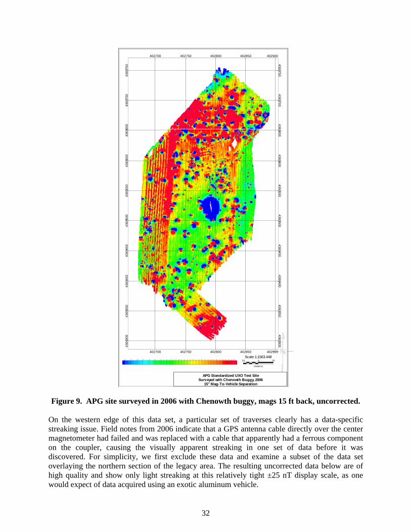
We covered 5.5 acres in the north section of the APG site. This was a somewhat smaller area than planned. This was because the portion of the legacy area in the southern section of the Standardized Test SiteCthe part to the south of the Indirect Fire areaCwas not always available because of live weapons testing at a section of APG just south of the Standardized Test Site. However it was more than enough area to collect sufficient data for the performance objectives. Figures 9-19 show:

Data acquired in 2006 with the Chenowth vehicle

o With no corrections o With a bidirectional correction applied o With a nominal 6 sec median filter applied.

Data acquired in 2009 with the COTS vehicle

o With no corrections o With a bidirectional correction applied o With a nominal 6 sec median filter applied o With the median filter window length varied to measure the effect on

target amplitude and spatial extent. 2006 Data with Chenowth Vehicle The scale for all image displays below is a relatively tight ± 25nT. First, we examine uncorrected data acquired with VSEMS in 2006 using the Chenowth aluminum buggy.

32

43

693

00

43

693

50

43

694

00

43

694

50

43

695

00

43

695

50

43

696

00

43

696

50

43

697

00

43

697

50

43

693

00

43

693

50

43

694

00

43

694

50

43

695

00

43

695

50

43

696

00

43

696

50

43

697

00

43

697

50

402700 402750 402800 402850 402900

402700 402750 402800 402850 402900

25 0 25

(meters)

Scale 1:1563.448

APG Standardized UXO Test SiteSurveyed with Chenowth Buggy, 2006

15" Mag-To-Vehicle Separation

- 23. 7 - 21. 2 - 18. 6 - 16. 0 - 13. 5 - 10. 9 - 8. 3 - 7. 1 - 5. 8 - 4. 5 - 3. 2 - 1. 9 - 0. 6 0. 6 1. 9 3. 2 4. 5 5. 8 7. 1 8. 3 9. 6 10. 9 12. 2 13. 5 14. 7 16. 0 17. 3 18. 6 19. 9 21. 2 22. 4 23. 7

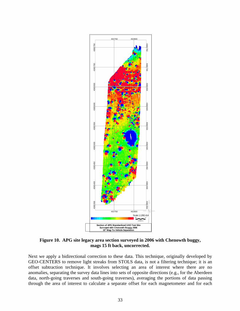
Figure 9. APG site surveyed in 2006 with Chenowth buggy, mags 15 ft back, uncorrected. On the western edge of this data set, a particular set of traverses clearly has a data-specific streaking issue. Field notes from 2006 indicate that a GPS antenna cable directly over the center magnetometer had failed and was replaced with a cable that apparently had a ferrous component on the coupler, causing the visually apparent streaking in one set of data before it was discovered. For simplicity, we first exclude these data and examine a subset of the data set overlaying the northern section of the legacy area. The resulting uncorrected data below are of high quality and show only light streaking at this relatively tight ±25 nT display scale, as one would expect of data acquired using an exotic aluminum vehicle.

33

43

69

35

04

36

94

00

43

69

45

04

36

95

00

43

69

55

04

36

96

00

43

69

65

04

36

97

00

43

69

75

04

36

93

50

43

69

40

04

36

94

50

43

69

50

04

36

95

50

43

69

60

04

36

96

50

43

69

70

04

36

97

50

402750 402800

402750 402800

25 0

(meters)

Scale 1:1392.414

Section of APG Standardized UXO Test SiteSurveyed with Chenowth Buggy, 2006


- 2 3.7 - 2 1.2 - 1 8.6 - 1 6.0 - 1 3.5 - 1 0.9 - 8.3 - 7.1 - 5.8 - 4.5 - 3.2 - 1.9 - 0.6 0 .6 1 .9 3 .2 4 .5 5 .8 7 .1 8 .3 9 .6 1 0.9 1 2.2 1 3.5 1 4.7 1 6.0 1 7.3 1 8.6 1 9.9 2 1.2 2 2.4 2 3.7

Figure 10. APG site legacy area section surveyed in 2006 with Chenowth buggy, mags 15 ft back, uncorrected.

Next we apply a bidirectional correction to these data. This technique, originally developed by GEO-CENTERS to remove light streaks from STOLS data, is not a filtering technique; it is an offset subtraction technique. It involves selecting an area of interest where there are no anomalies, separating the survey data lines into sets of opposite directions (e.g., for the Aberdeen data, north-going traverses and south-going traverses), averaging the portions of data passing through the area of interest to calculate a separate offset for each magnetometer and for each

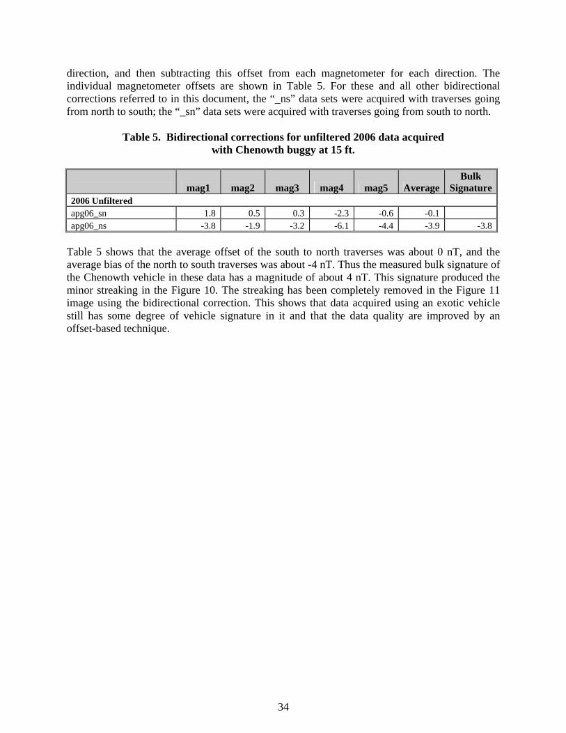
34

direction, and then subtracting this offset from each magnetometer for each direction. The individual magnetometer offsets are shown in Table 5. For these and all other bidirectional corrections referred to in this document, the “_ns” data sets were acquired with traverses going from north to south; the “_sn” data sets were acquired with traverses going from south to north.

Table 5. Bidirectional corrections for unfiltered 2006 data acquired with Chenowth buggy at 15 ft.

mag1 mag2 mag3 mag4 mag5 Average Bulk

Signature2006 Unfiltered apg06_sn 1.8 0.5 0.3 -2.3 -0.6 -0.1 apg06_ns -3.8 -1.9 -3.2 -6.1 -4.4 -3.9 -3.8

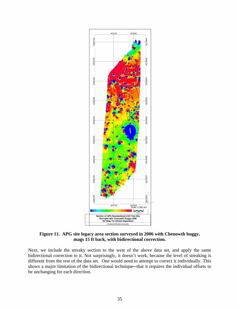
Table 5 shows that the average offset of the south to north traverses was about 0 nT, and the average bias of the north to south traverses was about -4 nT. Thus the measured bulk signature of the Chenowth vehicle in these data has a magnitude of about 4 nT. This signature produced the minor streaking in the Figure 10. The streaking has been completely removed in the Figure 11 image using the bidirectional correction. This shows that data acquired using an exotic vehicle still has some degree of vehicle signature in it and that the data quality are improved by an offset-based technique.

35

43

69

35

04

36

94

00

43

69

45

04

36

95

00

43

69

55

04

36

96

00

43

69

65

04

36

97

00

43

69

75

04

36

93

50

43

69

40

04

36

94

50

43

69

50

04

36

95

50

43

69

60

04

36

96

50

43

69

70

04

36

97

50

402750 402800

402750 402800

25 0

(meters)

Scale 1:1392.414


15" Mag-To-Vehicle SeparationCorrected Bidirectionally

Figure 11. APG site legacy area section surveyed in 2006 with Chenowth buggy,

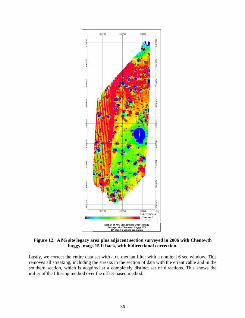
mags 15 ft back, with bidirectional correction. Next, we include the streaky section to the west of the above data set, and apply the same bidirectional correction to it. Not surprisingly, it doesn’t work, because the level of streaking is different from the rest of the data set. One would need to attempt to correct it individually. This shows a major limitation of the bidirectional techniqueCthat it requires the individual offsets to be unchanging for each direction.

36

25 0

(meters)

Scale 1:1392.414



- 23.7 - 21.2 - 18.6 - 16.0 - 13.5 - 10.9 - 8.3 - 7.1 - 5.8 - 4.5 - 3.2 - 1.9 - 0.6 0. 6 1. 9 3. 2 4. 5 5. 8 7. 1 8. 3 9. 6 10. 9 12. 2 13. 5 14. 7 16. 0 17. 3 18. 6 19. 9 21. 2 22. 4 23. 7

43

69

35

04

36

94

00

43

69

45

04

36

95

00

43

69

55

04

36

96

00

43

69

65

04

36

97

00

43

69

75

04

36

93

50

43

69

40

04

36

94

50

43

69

50

04

36

95

50

43

69

60

04

36

96

50

43

69

70

04

36

97

50

402700 402750 402800

402700 402750 402800

Figure 12. APG site legacy area plus adjacent section surveyed in 2006 with Chenowth buggy, mags 15 ft back, with bidirectional correction.

Lastly, we correct the entire data set with a de-median filter with a nominal 6 sec window. This removes all streaking, including the streaks in the section of data with the errant cable and in the southern section, which is acquired at a completely distinct set of directions. This shows the utility of the filtering method over the offset-based method.

37

43

693

00

43

693

50

43

694

00

43

694

50

43

695

00

43

695

50

43

696

00

43

696

50

43

697

00

43

697

50

43

693

00

43

693

50

43

694

00

43

694

50

43

695

00

43

695

50

43

696

00

43

696

50

43

697

00

43

697

50

402700 402750 402800 402850 402900

402700 402750 402800 402850 402900

25 0 25

(meters)

Scale 1:1563.448


15' Mag-To-Vehicle Separation6 Second De-median Filter

-23.7 -19.9 -16.0 -12.2 -8.3 -5.8 -3.2 -0.6 1.9 4.5 7.1 9.6 12.2 16.0 19.9 23.7

Figure 13. APG site legacy area plus adjacent section surveyed in 2006 with Chenowth buggy, mags 15 ft back, with de-median correction.

Visually, there are no streaks in these data, but we can apply the same method of measurement as we did above: dividing the data into south-to-north traverses and north-to-south traverses, evaluating the readings per sensor in a quiet area of interest, and averaging the results. We do not apply the bidirectional corrections; we merely generate them to populate Table 6, which shows that the bulk signature remaining after filtering is essentially zero.

38

Table 6. Bidirectional corrections for filtered 2006 data acquired with Chenowth buggy at 15 ft.


Signature2006 Filtered apg06_sn 0.1 0.1 0.1 0.0 0.0 0.1 apg06_ns 0.0 0.1 0.1 0.1 0.1 0.1 0.0

2009 Data with COTS VehicleCAggressive Configuration (magnetometers 15 ft back, skidplate installed) Next we look at data acquired in 2009 over the legacy area with the COTS vehicle in its more aggressive configuration (with the magnetometers 15 ft behind the vehicle and with the steel skid plate installed). The streaks from the directionally varying signature in adjacent traverses acquired 180E apart are plainly visible. Unlike the uncorrected 2006 Chenowth data, which had only minor streaking, the quality of the uncorrected data acquired with the COTS vehicle is clearly impaired without some sort of streak removal.

39

43

69

44

04

36

94

60

43

69

48

04

36

95

00

43

69

52

04

36

95

40

43

69

56

04

36

95

80

43

69

60

04

36

96

20

43

69

64

04

36

96

60

43

69

68

04

36

97

00

43

69

72

0

43

69

44

04

36

94

60

43

69

48

04

36

95

00

43

69

52

04

36

95

40

43

69

56

04

36

95

80

43

69

60

04

36

96

20

43

69

64

04

36

96

60

43

69

68

04

36

97

00

43

69

72

0

402660 402680 402700 402720 402740 402760 402780 402800

402660 402680 402700 402720 402740 402760 402780 402800

10 0 10 20

(meters)

Scale 1:932.7586

Section of APG Standardized UXO Test SiteSurveyed with COTS Vehicle, 2009

15" Mag-To-Vehicle Separation, Plate Attached

-23.7 -21.2 -18.6 -16.0 -13.5 -10.9 -8.3 -7.1 -5.8 -4.5 -3.2 -1.9 -0.6 0.6 1.9 3.2 4.5 5.8 7.1 8.3 9.6 10.9 12.2 13.5 14.7 16.0 17.3 18.6 19.9 21.2 22.4 23.7

Figure 14. Legacy area surveyed with COTS vehicle, mags 15 ft back, skidplate attached, uncorrected.

Next we apply the same kind of bidirectional streak correction described above to the 2009 COTS vehicle data. Unlike the 2006 data, which were acquired in discrete lines (pausing data acquisition while the vehicle turned around), the 2009 data was acquired in one long continuous line, with the turnarounds intentionally kept in the data set so we could see the effect of the vehicle. To perform the bidirectional correction, we first need to run a program that chops up the single long data line into distinct lines in each of the primary directions (Oasis will do this as

40

well, through the Database Tools | Line Tools | Split on XY option). Then the correction is performed as described above. The offset values are shown in Table 7.

Table 7. Bidirectional corrections for unfiltered 2009 COTS vehicle data acquired at 15 ft with skidplate.

mag1 mag2 mag3 mag4 mag5 Average Bulk Signature

2009 Aggressive Unfiltered apg09_15p_sn -22.8 -22.6 -24.3 -32.5 -28.0 -26.1 apg09_15p_ns -7.3 -0.8 -3.6 -11.2 -7.3 -6.0 20.0

From here we see that, using the COTS vehicle in its more aggressive configuration, the average bias of the south-to-north traverses is about -26 nT; the average bias of the north-to-south traverses is about -6 nT. This yields a bulk signature of about 20 nT, as compared with 4 nT with the Chenowth vehicle. With the individual biases subtracted off, the resulting data in the image below are streak-free. This provides confirmation that high quality magnetometer data can be acquired using a COTS vehicle and applying a simple bidirectional offset-based correction.

41

43

69

44

04

36

94

60

43

69

48

04

36

95

00

43

69

52

04

36

95

40

43

69

56

04

36

95

80

43

69

60

04

36

96

20

43

69

64

04

36

96

60

43

69

68

04

36

97

00

43

69

72

0

43

69

44

04

36

94

60

43

69

48

04

36

95

00

43

69

52

04

36

95

40

43

69

56

04

36

95

80

43

69

60

04

36

96

20

43

69

64

04

36

96

60

43

69

68

04

36

97

00

43

69

72

0

402660 402680 402700 402720 402740 402760 402780 402800

402660 402680 402700 402720 402740 402760 402780 402800

10 0 10 20

(meters)

Scale 1:928.9655


15" Mag-To-Vehicle Separation, Plate AttachedCorrected Bidirectionally

- 23. 7 - 21. 2 - 18. 6 - 16. 0 - 13. 5 - 10. 9 - 8. 3 - 7. 1 - 5. 8 - 4. 5 - 3. 2 - 1. 9 - 0. 6 0. 6 1. 9 3. 2 4. 5 5. 8 7. 1 8. 3 9. 6 10. 9 12. 2 13. 5 14. 7 16. 0 17. 3 18. 6 19. 9 21. 2 22. 4 23. 7

Figure 15. Legacy area surveyed with COTS vehicle, mags 15 ft back, skidplate attached, with bidirectional correction.

The usefulness of the bidirectional correction, however, has limits. Firstly, it requires data to be collected in sets of uniform direction. This is not a problem for grid surveys in obstructed areas, but in real-world production geophysics, sites are sometimes oddly shaped, have obstacles that must be driven around, or require patchwork fill-ins that make the bidirectional technique cumbersome or useless. In addition, experience has shown that, even on large regularly shaped sites where physical tire tracks on the ground are the main source of guidance, the survey direction will not remain invariant and will instead begin to drift as tire tracks are imperfectly

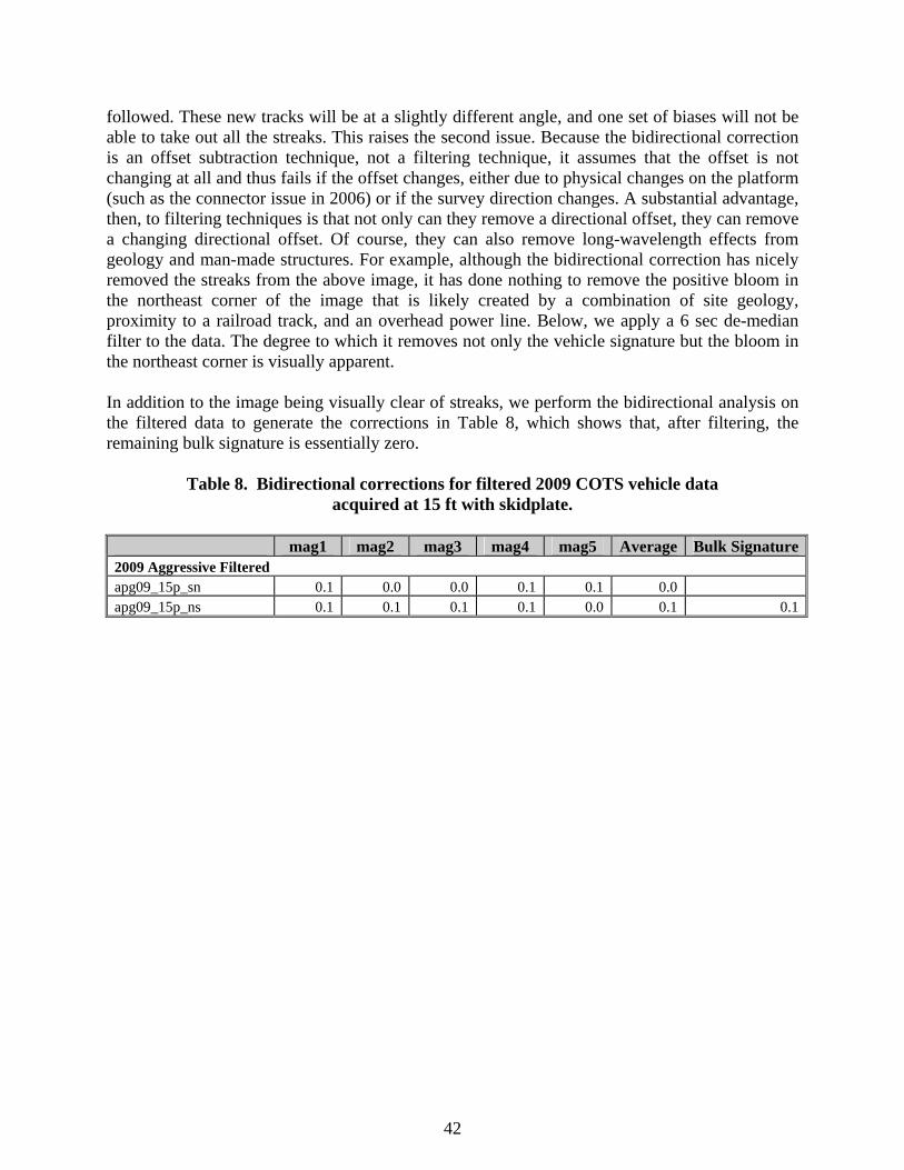
42

followed. These new tracks will be at a slightly different angle, and one set of biases will not be able to take out all the streaks. This raises the second issue. Because the bidirectional correction is an offset subtraction technique, not a filtering technique, it assumes that the offset is not changing at all and thus fails if the offset changes, either due to physical changes on the platform (such as the connector issue in 2006) or if the survey direction changes. A substantial advantage, then, to filtering techniques is that not only can they remove a directional offset, they can remove a changing directional offset. Of course, they can also remove long-wavelength effects from geology and man-made structures. For example, although the bidirectional correction has nicely removed the streaks from the above image, it has done nothing to remove the positive bloom in the northeast corner of the image that is likely created by a combination of site geology, proximity to a railroad track, and an overhead power line. Below, we apply a 6 sec de-median filter to the data. The degree to which it removes not only the vehicle signature but the bloom in the northeast corner is visually apparent. In addition to the image being visually clear of streaks, we perform the bidirectional analysis on the filtered data to generate the corrections in Table 8, which shows that, after filtering, the remaining bulk signature is essentially zero.

Table 8. Bidirectional corrections for filtered 2009 COTS vehicle data acquired at 15 ft with skidplate.

mag1 mag2 mag3 mag4 mag5 Average Bulk Signature

2009 Aggressive Filtered apg09_15p_sn 0.1 0.0 0.0 0.1 0.1 0.0 apg09_15p_ns 0.1 0.1 0.1 0.1 0.0 0.1 0.1

43

43

69

44

04

36

94

60

43

69

48

04

36

95

00

43

69

52

04

36

95

40

43

69

56

04

36

95

80

43

69

60

04

36

96

20

43

69

64

04

36

96

60

43

69

68

04

36

97

00

43

69

72

0

43

69

44

04

36

94

60

43

69

48

04

36

95

00

43

69

52

04

36

95

40

43

69

56

04

36

95

80

43

69

60

04

36

96

20

43

69

64

04

36

96

60

43

69

68

04

36

97

00

43

69

72

0

402660 402680 402700 402720 402740 402760 402780 402800

402660 402680 402700 402720 402740 402760 402780 402800

10 0 10 20

(meters)

Scale 1:932.7586


15' Mag-To-Vehicle Separation, Plate InstalledSix Second De-median Filter

-23.7 -21.2 -18.6 -16.0 -13.5 -10.9 -8.3 -7.1 -5.8 -4.5 -3.2 -1.9 -0.6 0.6 1.9 3.2 4.5 5.8 7.1 8.3 9.6 10.9 12.2 13.5 14.7 16.0 17.3 18.6 19.9 21.2 22.4 23.7

Figure 16. Legacy area surveyed with COTS vehicle, mags 15 ft back, skidplate installed, with de-median filter correction.

2009 Data with COTS VehicleCConservative Configuration (magnetometers 17 ft back, skidplate removed) Next we examine the 2009 COTS vehicle data in its more conservative configurationCwith the magnetometers moved back to 17 ft and with the steel skidplate removed. Figure 17 shows some light streaking, but the streaks are of a lower magnitude than those in the more aggressive configuration in Figure 16.

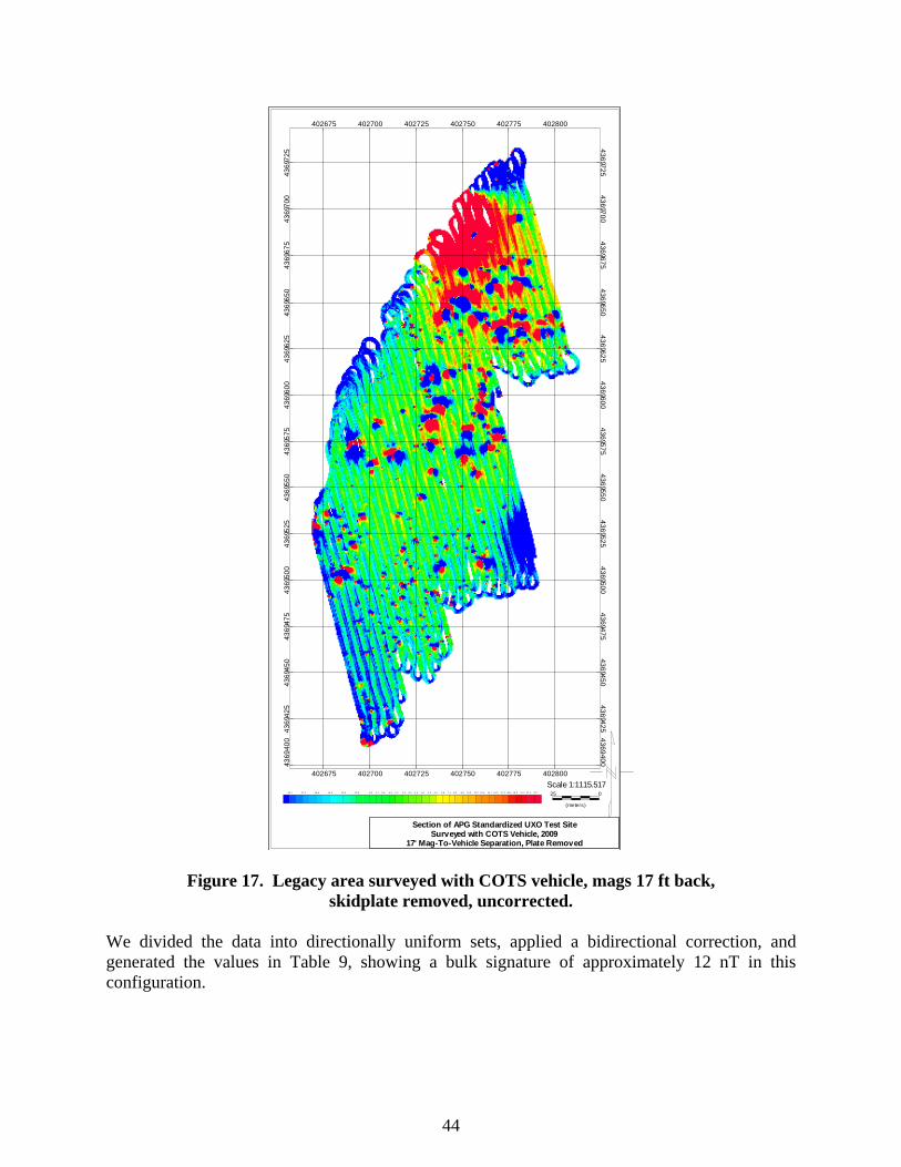
44

43

69

40

04

36

942

54

36

945

04

36

947

54

36

950

04

36

952

54

36

955

04

36

957

54

36

960

04

36

962

54

36

965

04

36

967

54

36

970

04

36

972

5

43

69

40

04

36

942

54

36

945

04

36

947

54

36

950

04

36

952

54

36

955

04

36

957

54

36

960

04

36

962

54

36

965

04

36

967

54

36

970

04

36

972

5

402675 402700 402725 402750 402775 402800

402675 402700 402725 402750 402775 402800

25 0

(meters)

Scale 1:1115.517


17' Mag-To-Vehicle Separation, Plate Removed

- 23. 7 - 21. 2 - 18. 6 - 16. 0 - 13. 5 - 10. 9 - 8. 3 - 7. 1 - 5. 8 - 4. 5 - 3. 2 - 1. 9 - 0. 6 0. 6 1. 9 3. 2 4. 5 5. 8 7. 1 8. 3 9. 6 10. 9 12. 2 13. 5 14. 7 16. 0 17. 3 18. 6 19. 9 21. 2 22. 4 23. 7

Figure 17. Legacy area surveyed with COTS vehicle, mags 17 ft back, skidplate removed, uncorrected.

We divided the data into directionally uniform sets, applied a bidirectional correction, and generated the values in Table 9, showing a bulk signature of approximately 12 nT in this configuration.

45

Table 9. Bidirectional corrections for unfiltered 2009 COTS vehicle data acquired at 17 ft without skidplate.


Signature2009 Conservative Unfiltered

apg09_17n_sn -10.2 -12.1 -9.2 -17.4 -12.3 -12.3

apg09_17n_ns 0.9 1.4 2.7 -6.0 -1.1 -0.4 11.9

Data with the bidirectional correction applied are shown in Figure 18.

46

43

69

40

04

36

94

25

43

69

45

04

36

94

75

43

69

50

04

36

95

25

43

69

55

04

36

95

75

43

69

60

04

36

96

25

43

69

65

04

36

96

75

43

69

70

04

36

97

25

43

69

40

04

36

94

25

43

69

45

04

36

94

75

43

69

50

04

36

95

25

43

69

55

04

36

95

75

43

69

60

04

36

96

25

43

69

65

04

36

96

75

43

69

70

04

36

97

25

402675 402700 402725 402750 402775 402800

402675 402700 402725 402750 402775 402800

25 0

(meters)

Scale 1:1115.517


17' Mag-To-Vehicle Separation, Plate RemovedBidirectional Correction

- 23. 7 - 21. 2 - 18. 6 - 16. 0 - 13. 5 - 10. 9 - 8. 3 - 7. 1 - 5. 8 - 4. 5 - 3. 2 - 1. 9 - 0. 6 0. 6 1. 9 3. 2 4. 5 5. 8 7. 1 8. 3 9. 6 10. 9 12. 2 13. 5 14. 7 16. 0 17. 3 18. 6 19. 9 21. 2 22. 4 23. 7

Figure 18. Legacy area surveyed with COTS vehicle, mags 17 ft back, skidplate removed, with bidirectional correction.

The bidirectionally corrected data shown in Figure 18 exhibit some light streaking visible near the center of the image. We attribute these streaks to the reliance of the correction on rigorously uniform direction in both the survey data and in the data used to generate the correction. In Figure 19, we apply the standard 6 sec de-median filter instead; it removes the light streaking in the middle and most of the cultural and geological bloom in the northeast corner. Table 10 shows the bulk signature data, again showing that after filtering, the bulk signature is essentially zero.

47

Table 10. bidirectional corrections for filtered 2009 COTS vehicle data acquired at 17 ft without skidplate.


Signature2009 Conservative Filtered apg09_17n_sn 0.0 0.0 0.0 0.0 0.1 0.0 apg09_17n_ns 0.0 0.1 0.1 0.1 0.1 0.1 0.1

48

43

69

40

04

369

42

54

369

45

04

369

47

54

369

50

04

369

52

54

369

55

04

369

57

54

369

60

04

369

62

54

369

65

04

369

67

54

369

70

04

369

72

5

43

69

40

04

369

42

54

369

45

04

369

47

54

369

50

04

369

52

54

369

55

04

369

57

54

369

60

04

369

62

54

369

65

04

369

67

54

369

70

04

369

72

5

402675 402700 402725 402750 402775 402800

402675 402700 402725 402750 402775 402800

25 0

(meters)

Scale 1:1115.517


17' Mag-To-Vehicle Separation, Plate Removed6 Second De-median Filter

-23.7 -19.9 -16.0 -12.2 -8.3 -5.8 -3.2 -0.6 1.9 4.5 7.1 9.6 12.2 16.0 19.9 23.7

Figure 19. Legacy area surveyed with COTS vehicle, mags 17 ft back, skidplate removed, with de-median filter correction.

8.4.3 Bulk Signature Summary

In Table 11, we summarize the bulk signature of the octant data and the survey data (uncorrected and de-median filtered with a nominal 6 sec window) for the configurations we have described above. We position the octant and survey data measurements from like configurations in adjacent lines so their consistency can be seen. As per the above tables, the remaining bulk signature after filtering is essentially zero.

49

Table 11. Bulk signature summary.

Vehicle-Sensor Separation (ft) Octant or

Survey Bulk Signature, Unfiltered (nT)

Bulk Signature, Filtered (nT)

2006, 15 ft, Chenowth Survey 3.8 0.0 2009, 15 ft, COTS, skidplate removed Octant 15.0 2009, 15 ft, COTS, skidplate installed Octant 22.1 2009, 15 ft, COTS, skidplate installed Survey 20.0 0.1 2009, 17 ft, COTS, skidplate removed Octant 10.3 2009, 17 ft, COTS, skidplate removed Survey 11.9 0.1 2009, 17 ft, COTS, skidplate installed Octant 7.9

8.4.4 Effect of De-Median Filter Window Length

The Final Report contains a lengthy discussion of the effect of the de-median filter’s window length on anomaly amplitude and spatial extent. It is summarized here. To quantify the effect of the de-median filter, we selected nine targets of a variety of sizes (spatial anomaly extent) from the data set. For each target, for each of the 15 median filter window filter lengths, we extracted the best time-series profile over that target and tabulated the target’s amplitude and the full width at half the maximum value. These are shown in both tabular (Table 12) and graphical (Figure 20) form below. When looking at the peak amplitude, the graphs level out for most of the nine objects at approximately 3 sec. The exception is object #2, which is the object whose anomaly has the largest spatial extent; the curve for this object flattens after approximately 6 sec. To evaluate compliance with the performance objective of not altering the anomaly by more than 15%, we take the most slowly changing item (item2); its strength is within 15% of its asymptotic value after 4 sec, and within 1% after 6 sec.

Table 12. Nine objects, anomaly peak amplitude as a function of median filter window length.

Item1 Item2 Item3 Item4 Item5 Item6 Item7 Item8 Item9

1 458.5 385.5 1247.2 206.1 3861.4 369.4 141.1 510.2 322.52 1009.1 874.0 1959.7 546.4 6841.7 914.7 375.5 854.7 801.53 1386.3 1376.3 2146.2 740.6 7490.8 1180.7 505.7 969.0 1091.64 1579.8 1682.7 2197.2 833.7 7616.3 1285.4 553.6 1013.8 1219.45 1659.9 1871.5 2214.7 881.9 7647.0 1328.9 565.4 1032.0 1255.56 1691.6 1972.0 2217.2 906.0 7649.7 1353.2 568.8 1041.0 1272.87 1707.7 2022.9 2218.8 920.7 7649.7 1369.2 568.8 1042.6 1276.78 1714.6 2052.0 2220.4 925.3 7649.7 1378.0 568.8 1042.6 1277.79 1718.2 2066.8 2222.9 928.0 7649.7 1379.6 568.8 1042.6 1278.3

10 1720.4 2075.4 2224.5 929.1 7649.7 1380.8 568.8 1043.9 1278.511 1721.1 2080.6 2226.2 929.1 7649.7 1381.0 568.8 1046.5 1278.912 1723.9 2082.0 2226.7 929.1 7649.7 1380.9 568.8 1048.9 1278.913 1725.3 2082.8 2227.2 929.1 7649.5 1380.5 568.8 1049.9 1278.914 1729.9 2083.2 2227.7 929.1 7649.1 1379.9 568.8 1051.3 1278.915 1732.1 2083.4 2228.0 929.1 7648.4 1379.9 568.9 1052.5 1278.9

50

0

1000

2000

3000

4000

5000

6000

7000

8000

9000

0 2 4 6 8 10 12 14 16

Median Filter Window Length (seconds)

Pea

k V

alu

e (n

T)

item1

item2

item3

item4

item5

item6

item7

item8

item9

Figure 20. Nine objects, anomaly peak amplitude as a function of

median filter window length. For anomaly size (full width at half max), most of the graphs visually level out at approximately 6 sec, with the graphs of objects 1, 2, and 3 taking slightly longer to flatten. To evaluate the performance objective of not altering the anomaly by more than 15%, we take the most slowly changing item (item2); its size is within 15% of its asymptotic value after 4 sec, and within 1% after 6 sec.

Table 13. Nine objects, anomaly full width at half max as a function of median filter window length.

Seconds Item1 Item2 Item3 Item4 Item5 Item6 Item7 Item8 Item9

1 0.34 0.35 0.39 0.66 0.5 0.46 0.46 0.38 0.52 2 0.84 0.74 0.53 1.23 0.79 0.86 0.82 0.6 0.84 3 1.11 1.14 0.56 1.4 0.83 1.02 0.98 0.65 1.03 4 1.22 1.29 0.6 1.52 0.86 1.1 1.03 0.67 1.11 5 1.28 1.4 0.6 1.78 0.86 1.12 1.05 0.69 1.13 6 1.3 1.45 0.6 1.81 0.86 1.12 1.05 0.71 1.26 7 1.3 1.47 0.6 1.83 0.86 1.14 1.05 0.71 1.26 8 1.32 1.48 0.6 1.85 0.86 1.14 1.05 0.71 1.26 9 1.32 1.5 0.6 1.85 0.86 1.14 1.05 0.71 1.26

10 1.32 1.5 0.6 1.85 0.86 1.14 1.05 0.71 1.26 11 1.32 1.5 0.6 1.85 0.86 1.14 1.05 0.71 1.26 12 1.32 1.5 0.6 1.85 0.86 1.14 1.05 0.71 1.26 13 1.32 1.5 0.6 1.85 0.86 1.14 1.05 0.71 1.26 14 1.32 1.5 0.6 1.85 0.86 1.14 1.05 0.71 1.26 15 1.32 1.5 0.6 1.85 0.86 1.14 1.05 0.71 1.26

51

0

0.2

0.4

0.6

0.8

1

1.2

1.4

1.6

1.8

2

0 2 4 6 8 10 12 14 16

Median Filter Window Length (seconds)

Fu

ll W

idth

at

Hal

f M

ax (

seco

nd

s)

item1

item2

item3

item4

item5

item6

item7

item8

item9

Figure 21. Nine objects, anomaly full width at half max as a function of

median filter window length. To summarize the above results, we take the two tables, calculate each value as a percentage of the asymptotic value, and average across all nine objects. The 6 sec value nominally used is highlighted.

Table 14. Summary of filter effects on amplitude and width.

Window Amplitude Width 1 66.8% 57.0% 2 31.9% 26.2% 3 14.2% 13.1% 4 6.4% 6.9% 5 3.1% 3.2% 6 1.6% 1.0% 7 0.8% 0.5% 8 0.5% 0.1% 9 0.3% 0.0%

10 0.2% 0.0% 11 0.1% 0.0% 12 0.1% 0.0% 13 0.1% 0.0% 14 0.0% 0.0% 15 0.0% 0.0%

Together, these tables and graphs show that both the amplitude and spatial extent of the de-median filtered anomalies meet the demonstration’s metric (they are within 15% of the

52

asymptotic value) when a de-median filter of at least a 4 sec time window is used. Further, both the amplitude and size are within 2% of their asymptotic values when a 6 sec window is used. Certainly using a median filter in the 6 sec range does not have a deleterious effect on anomaly amplitude and size.

8.4.5 Effect of Rough Terrain

Although the effect of the vehicle changes primarily with the vehicle’s orientation relative to north, it also changes as the vehicle and the sensor platform both pitch and roll over rough terrain. The question is whether, for a given vehicle and sensor separation, pitch and roll effects are large enough to be problematic. In data acquired using a variety of COTS vehicles at a variety of sensor separations during the project’s testing at Fort Devens, we found that, when the vehicle had too strong a signature or the sensors were too close, we saw this effect as a “clouding” of the dataClow-level spatially diffuse anomalies that were plainly visible after the slowly changing directional component had been removed with a de-median filter. For the APG demonstration, we tried to correlate such possible artifacts with rough patches of terrain by acquiring GPS coordinates over certain particularly rough sections of the site. This was done by having a passenger take notes while the driver was covering planned traverses. For example, a sample note might read “north end of line 5 very rough.” After the survey was completed, the driver went back to the notated areas and recorded their GPS coordinates to see if we could correlate these rough sections with visible artifacts in the filtered data such as the “cloudy” artifacts we saw with some vehicles at Devens. In Figures 22 and 23, the rough sections at APG are shown as the black lines. The images of 6 sec de-median filtered data, like all other images in this document, are shown at ± 25nT, but the point at which green transitions to yellow has been pushed down to zero in order to visually highlight small positive changes in the data.

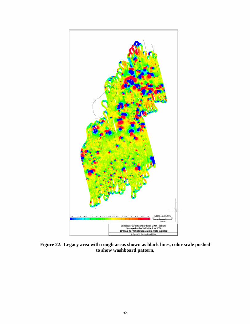
53

10 0 10 20

(meters)

Scale 1:932.7586


15' Mag-To-Vehicle Separation, Plate Installed6 Second De-median Filter

-23.7 -19.9 -16.0 -12.2 -8.3 -5.8 -3.2 -0.6 1.9 4.5 7.1 9.6 12.2 16.0 19.9 23.7

Figure 22. Legacy area with rough areas shown as black lines, color scale pushed to show washboard pattern.

54

Figure 23. Blowup to show washboard pattern. We see no such “cloudy” artifacts in the more aggressive 15 ft data, nor in the more conservative 17 ft data. What we do see, however, is a down-track washboard artifact, periodic and coherent across all sensors, of approximately 3 nT peak to peak. The second image is zoomed in to better show the artifact. The washboard pattern appears to be uncorrelated, with the black lines indicating rough areas. The pattern is almost certainly due to the ferrous beads in the tires on the buggy. The physical distance between the anomaly peaks is approximately 1.8 m, which is almost exactly the circumference of the vehicle’s 1.875 ft (0.57 m) high tires. The fact that the artifact ebbs and flows somewhat is probably due to constructive interference between the signals from the steel beads on the vehicle’s two rear tires. We had demagnetized the eight beads on the four tires when we purchased the vehicle, but that was nearly 18 months before the APG survey. It is likely that they need to be demagnetized again. Note that both MTADS’ and VSEMS’ practice has been to employ tires with their steel beads removed on the survey platform, as these are very close to the magnetometers, but the tires on the survey vehicle must bear the weight of the vehicle, so we have been demagnetizing, not removing, the beads in the vehicle’s tires. Even though we do not see any artifacts that we would associate with pitch and roll over rough terrain, a statistical comparison was made between data from an anomaly-free area in the rough section in the wet area at the northern edge, and data from an anomaly-free area that was not

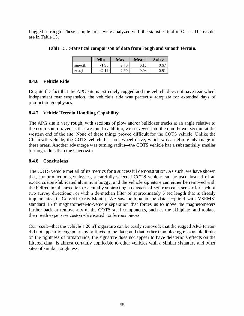
55

flagged as rough. These sample areas were analyzed with the statistics tool in Oasis. The results are in Table 15.

Table 15. Statistical comparison of data from rough and smooth terrain.

Min Max Mean Stdev smooth -1.90 2.48 0.12 0.67rough -2.14 2.89 0.04 0.81

8.4.6 Vehicle Ride

Despite the fact that the APG site is extremely rugged and the vehicle does not have rear wheel independent rear suspension, the vehicle’s ride was perfectly adequate for extended days of production geophysics.

8.4.7 Vehicle Terrain Handling Capability

The APG site is very rough, with sections of plow and/or bulldozer tracks at an angle relative to the north-south traverses that we ran. In addition, we surveyed into the muddy wet section at the western end of the site. None of these things proved difficult for the COTS vehicle. Unlike the Chenowth vehicle, the COTS vehicle has four wheel drive, which was a definite advantage in these areas. Another advantage was turning radiusCthe COTS vehicle has a substantially smaller turning radius than the Chenowth.

8.4.8 Conclusions

The COTS vehicle met all of its metrics for a successful demonstration. As such, we have shown that, for production geophysics, a carefully-selected COTS vehicle can be used instead of an exotic custom-fabricated aluminum buggy, and the vehicle signature can either be removed with the bidirectional correction (essentially subtracting a constant offset from each sensor for each of two survey directions), or with a de-median filter of approximately 6 sec length that is already implemented in Geosoft Oasis Montaj. We saw nothing in the data acquired with VSEMS’ standard 15 ft magnetometer-to-vehicle separation that forces us to move the magnetometers further back or remove any of the COTS steel components, such as the skidplate, and replace them with expensive custom-fabricated nonferrous pieces. Our resultCthat the vehicle’s 20 nT signature can be easily removed; that the rugged APG terrain did not appear to engender any artifacts in the data; and that, other than placing reasonable limits on the tightness of turnarounds, the signature does not appear to have deleterious effects on the filtered dataCis almost certainly applicable to other vehicles with a similar signature and other sites of similar roughness.

57

9.0 COST ASSESSMENT

9.1 COST MODEL

The cost model is presented in Table 16.

Table 16. Cost model.

Cost Element Data Tracked during Demonstration Estimated Costs Instrument cost Component costs and integration costs

Engineering estimates based on current development Lifetime estimate Track consumables and repairs

$13,000

Mobilization and demobilization

Cost to mobilize to site (derived from demonstration costs)

$8100

Site preparation No unique requirements encountered Instrument setup costs

Unit cost to set up and calibrate Data requirements: Hours required Personnel required Frequency required

$275 2 hours 2 people One-time setup

Survey costs Unit cost per hectare Data requirements: Hours per hectare Personnel required

$641/hectare 1.8 hours/hectare 2 people

Detection data processing costs

Unit cost per hectare as function of anomaly density Data requirements: Time required Personnel required

No detection performed

Discrimination data processing

Unit cost per anomaly Time required Personnel required

No discrimination performed

Instrument Cost: This is the cost of the COTS vehicle. When SAIC purchased the Club Car 1550XRT UTV, it cost approximately $13,000. Mobilization and Demobilization: The cost to mobilize the vehicle, the towed array, and the two-man crew to APG for the demonstration was approximately $8100. Site Preparation: No site preparation above that which is necessary for any vehicle-towed array is required. Instrument Setup Costs: Vehicle towed arrays are typically shipped intact. The two-man crew routinely set the system up and began collecting data within an hour of arriving at a site. Thus we estimate the cost as two people for one hour each. Survey Costs: The survey costs are the same as any towed array (or, more specifically, the same as a towed array using an exotic custom-built vehicle), and these of course depend on many factors, including site topography, hours of access to the site, weather, and GPS problems. The

58

daily rate for the principal investigator (PI) and an equipment operator in the field was $2824/day. We surveyed the 5.5 acre (2.2 hectares) sections of the legacy area in about one-half a day. This was not intended to be a test of efficiency; survey lines were short, and additional nonsurvey tests such as octant tests were also run. Nonetheless, this survey rate comes out to be 4.4 hectares/day or 1.8 hours/hectare, at a cost of $641/hectare. Detection Data Processing Costs: Processing of VSEMS magnetometer data is similar to processing data from any other magnetometer array. The data must be de-spiked and background-leveled. The use of a COTS vehicle requires filtering the data to remove the directionally varying vehicle signature, but as we have shown, the same de-median filter that is traditionally employed to remove diurnal drift, long-wavelength geology, and small intermagnetometer offsets also removes vehicle signature. These steps are performed in Geosoft Oasis Montaj. VSEMS’ magnetometer data requires the additional step of notch-filtering out the instrument-specific 15 Hz hum (created by the 60 Hz ambient electrical hum aliasing at 15 Hz because it is sampled at 75 Hz). We usually perform this step in our own software, but Oasis is capable of notch-filtering the data as well. Because our magnetometer data is 1PPS-triggered, it never requires latency correction. The magnetometer data can be read into Oasis and thresholded to generate a mag dig sheet. Discrimination Data Processing Costs: The scope of this project, to date, has not included discrimination processing.

9.2 COST DRIVERS

Any vehicle will require a certain amount of time to integrate sensors, electronics, GPS, and data acquisition components, but this time is not much different on COTS versus custom vehicles.

9.3 COST BENEFIT

The cost benefit comes from not having to spend $100,000 on a custom-built vehicle, and instead being able to spend closer to $13,000 on a COTS vehicle.

59

10.0 IMPLEMENTATION ISSUES

10.1 ENVIRONMENTAL AND REGULATORY ISSUES

Because the technology involves an already validated sensor for DGMCtotal field magnetometersCthere are no specific regulatory issues above those that apply to all DGM data. Any applicable regulatory issues involve detection and discrimination systems of all kinds (i.e., how clean is clean, etc) and are not specific to this project or technology.

10.2 END-USER ISSUES

Because the sensors are not only COTS but the very sensors already well-used for MEC DGM, there should not be serious impediments to use.

10.3 RELEVANT PROCUREMENT ISSUES

The vehicle, GPS, and magnetometers are COTS.

10.4 AVAILABILITY OF THE TECHNOLOGY

Any contractor can purchase the specified COTS Club Car 1550XRT vehicle (or a similar one) and use, along with COTS magnetometers and a GPS, to tow a magnetometer array of their own design.

10.5 SPECIALIZED SKILLS AND TRAINING

Because the sensors are not only COTS but the very sensors already well-used for MEC DGM, training is minimal. However, due to the number and variety of sources of noise (of which directionally varying magnetic signature is only one), background or experience in magnetometry is necessary to build a system that collects high-quality magnetometer data.

61

11.0 REFERENCES

SERDP ESTCP IRTC “Survey of Munitions Response Technologies,” 2008. Siegel, Robert. 2008. MM-0605 COTS Vehicles for Towed Array Magnetometry Demonstration

Plan, submitted to ESTCP Program Office 11/21/2008. Siegel, Robert. 2007. MM-0605 Vehicle Signature Report and Geophysical Procedures for

Vehicle Signature Measurement v3.doc, submitted to ESTCP Program Office 4/27/2007.

A-1

APPENDIX A

POINTS OF CONTACT

Point of Contact Organization

Phone Fax

E-Mail Role Rob Siegel SAIC, Inc.

7 Wells Ave Newton, MA 02459

Phone: 617-618-4662 Fax: 617-527-7592 [email protected]

Principal Investigator

Bob Selfridge U.S. Army Corps of Engineers, Huntsville 4820 University Square Huntsville, AL 35816-1822


Contracting Officer’s Technical Representative (COTR)

Dr. Herb Nelson ESTCP Program Office 901 North Stuart Street, Suite 303Arlington, VA 22203


ESTCP Munitions Management (MM) Program Manager

ESTCP Program Office

901 North Stuart StreetSuite 303Arlington, Virginia 22203

(703) 696-2117 (Phone)(703) 696-2114 (Fax)

E-mail: [email protected]

estcp cost and performance report cost and performance report ... (e.g., surface towed ordnance...

Documents