EQUILIBRIUM EFFECTS OF PAY

TRANSPARENCY∗

Zoe B. Cullen and Bobak Pakzad-Hurson

September 12, 2017

Click For Latest Version

The public conversation about increasing pay transparency largely ignores equilibrium effects,namely how it leads firms to change hiring and wage-setting policies and workers to adjust bar-gaining strategies. In this paper, we study these effects with a methodologically diverse approach.Our analysis combines longitudinal study of thousands of workers and employers facing differentlevels of pay transparency carrying out short term contract work, matched through an online la-bor platform, with a parsimonious equilibrium model of dynamic wage setting and negotiation.We find, theoretically and empirically, that increasing pay transparency can increase employment,decrease inequality in earnings, and shift surplus away from workers and toward their employer.Intermediate levels of pay transparency, achieved through a permissive environment to discuss rel-ative pay, can exacerbate the gender pay gap by virtue of network effects. External interventionmay be necessary to maintain a desirable level of transparency. We also conduct a field experimenton internet workers to investigate an alternative model in which wage compression is driven bysocial aversion to observed wage inequality. Our findings are consistent with our bargaining modelbut not with this alternative.

Keywords: Pay Transparency, Online Labor Market, Dynamic Bargaining, Field Experiment

JEL Classification Codes: C78, C93, D47, D83, J21, J33, J78, L22

∗We are very grateful for guidance from Susan Athey, Nick Bloom, Matt Jackson, Fuhito Kojima, EdLazear, Luigi Pistaferri, and Al Roth. We are indebted to James Flynn for technical support. We alsothank Mohammad Akbarpour, Jose Maria Barrero, Doug Bernheim, Eric Budish, Gabriel Carrol, ArunChandrasekhar, Isa Chaves, Bo Cowgill, Piotr Dworczak, Jack Fanning, Chiara Farronato, Bob Hall, Gre-gor Jarosch, Scott Kominers, Maciej Kotowski, Jon Levin, Shengwu Li, Erik Madsen, Davide Malacrino,Alejandro Martinez, Paul Milgrom, Muriel Niederle, Kareen Rozen, Ilya Segal, Isaac Sorkin, Jesse Shapiro,Takuo Sugaya, Emmanuel Vespa, Alistair Wilson, and various seminar attendees for helpful comments andsuggestions. We appreciate TaskRabbit for providing essential data access. Pakzad-Hurson acknowledgesfinancial support by the B.F. Haley and E.S. Shaw Dissertation Fellowship through a grant to the StanfordInstitute for Economic Policy Research. This paper subsumes two earlier drafts: Equal Pay for UnequalWork? and Is Pay Transparency a Good Idea?.

I. Introduction

Recent policy proposals to mitigate wage inequality include increasing pay transparency,

the amount of information workers have about each others wages.1 In many settings, the

first step has been to protect the right of co-workers to communicate pay information and

extend the time frame during which information from peers is permissible as court evidence

of pay discrimination. Following the signing of the 2009 Lilly Ledbetter Fair Pay Act, which

removed the statute of limitation for pay discrimination law suits, the federal government

has prohibited federal contractors from punishing workers who discuss pay at the workplace,

and several states have passed similar laws (including California and Massachusetts in 2016).

The stated purpose of these laws is to ensure that “victims of pay discrimination can effec-

tively challenge unequal pay” through negotiations, by informing them of their employer’s

willingness to pay for labor.2

However, the debate around pay transparency has paid little attention to equilibrium

effects, namely how firms might change their hiring and wage-setting policies in reaction to

transparency mandates and how workers might adjust their initial salary negotiations. It

also lacks a theory as to why some firms institute transparent pay structures in the absence

of any mandate at all. Our research aims to fill this void.

In this paper, we combine empirical analysis of local contract workers and their employers

over a four year horizon with a simple equilibrium model of dynamic wage negotiations

tailored to our empirical setting.

Workers and employers in our sample find each other and transact over an online platform,

TaskRabbit, which specializes in homogeneous, low-skill household tasks, and is active in 19

U.S. cities. The labor platform requires workers to bid for tasks but also allows for on-

the-job wage renegotiation leading employers to increase worker pay above the initial bids

through the platform. Our administrative data allows us to observe all bids, final wages, job

characteristics, and worker evaluations between 2010 and 2014.

The advent of large online spot markets for labor, like TaskRabbit, presents new oppor-

1The rise of wage inequality in the United States has been well documented (egs. Katz and Autor, 1999;Saez and Zucman, 2014; Piketty, 2014). Wage inequality has been linked to social and economic costs, suchas under-investment in human capital, misallocation of labor, and even infant mortality (Chen et al., 2014).Citing these economic and social costs, the Equal Pay Act of 1963 and subsequent legislation has increasinglymade it illegal for firms to pay workers based on factors other than performance.

These measures have not had the desired effect. In a well-cited statistic on wage inequality, full-timeworking American women currently earn on average 79% of what their male counterparts make (Blau andKahn, 2017). The gap is even larger for minority women. This is especially puzzling given convergence ineducational attainment. Indeed, the “unexplained” wage gap – the premium that cannot be explained aftercontrolling for observables – is approximately 8%, which is the highest it has been since the wage gap hasbeen noted in modern times (Blau and Kahn, 2017; Goldin, 2014).

2https://www.whitehouse.gov/blog/2009/01/25/now-comes-lilly-ledbetter accessed 11/7/2016.

1

tunities for the study of the wage determination process in an environment largely stripped

of career concerns and non-pecuniary benefits. In our empirical setting, pay transparency

varies by the ability of co-workers to communicate about pay on-the-job and by salary

announcements in the job posting. For example, in some multi-worker jobs, workers are

co-located packing boxes in the same office where they might share wage information, and

in others they are physically separated distributing marketing materials to different vendors

and are therefore unable to share information about their pay. Some employers choose to

use a transparent posted price to advertise their job, and others accept private bids from

interested workers.3

We assess the equilibrium costs and benefits of increasing pay transparency along three

dimensions: wage equality, employment rate, and profit split between workers and their

firm. We find that increasing transparency compresses the wages of similarly productive

workers. Some transparency increases employment, but too much reduces employment.

Higher transparency shifts expected surplus away from workers and toward the firm. We

also find that regulation may be necessary to ensure desirable transparency levels.

To support these claims, we propose and analyze a simple model of dynamic wage ne-

gotiations with three important bases: workers do not initially know their value to their

employer, workers are able to renegotiate their pay, and workers know how much they can

successfully demand in renegotiations upon learning the wages of their peers. Many specifics

of our model are based on institutional details of TaskRabbit (which we discuss in more

detail in Section IV.), nevertheless, its simplicity allows for many generalizations and ex-

tensions which preserve our main findings. While it is unfeasible to precisely describe every

market in a single paper, we believe that different formulations of our model may be good

approximations of some entry-level labor markets.

Formally, we study a continuous time game between a continuum of workers and a

firm(s).4 Bargaining takes the form of a directed take-it-or-leave-it (TIOLI) offer from a

worker to the firm, as in TaskRabbit, and akin to a phenomenon in the general labor market

where workers are asked to put forth their salary expectations to assess whether a match is

within the realm of possibilities. Employed workers are able to renegotiate with the firm

at will, but workers whose offers are rejected are permanently unmatched with the firm and

receive their heterogeneous, exogenous outside options.5 The level of pay transparency af-

3Wage bargaining and transfer of information via transparency are common in many labor markets.Hall and Krueger (2012) find that one-third of workers surveyed explicitly bargain when accepting a job,one-third face posted wages set by their employers, and nearly one-half report that previous wages were usedto set current wages. We observe both types of wage-setting, in similar proportions, in TaskRabbit.

4For simplicity, we present our model as containing a single firm. We generalize and extend our resultsto the case with multiple firms in Appendix D..

5Farrell and Greig (2016) find that online labor platform users earn on average one-third of their totalincome on platform, leading to heterogeneous outside options.

2

fects the rate at which information about co-worker pay arrives over time to employees. The

firm has a value for labor which is common across workers, but unknown to the workers.6

Therefore, seeing the pay of a higher paid co-worker is an indication of being underpaid.

We study the unique equilibrium in which the maximum wage offer a firm is willing to

accept is a linear function of its value for labor. In it, workers initially bid linear premia

over their outside options. Regardless of the level of transparency, workers will only choose

to renegotiate their wage once they learn the wage profile within the firm, at which point

in time they (successfully) demand pay that is equal to that of the highest earning worker.

Therefore, transparency causes an information externality; if a worker finds out that her

colleague receives a high wage, she will use this information to negotiate a higher wage for

herself. This affects the way that initial wages are set.

There are two major equilibrium effects of increasing transparency: a demand effect and

a supply effect. The demand effect reduces the firm’s willingness to pay for labor. Higher

transparency increases the chances of information spillovers over time across workers. As

such, the firm is able to commit to pay lower wages at the onset of the game. In equilibrium

with a fully secret pay structure (workers never learn the pay of their peers), the firm accepts

all wage offers that are less than the value of labor because there are no information spillovers.

With full transparency the firm chooses a posted wage below its value for labor that it pays

to all workers, analogously to a monopsonist maximizing its profits. The highest wage the

firm is willing to pay for labor is strictly decreasing in transparency.

With increased transparency, the supply effect dictates that workers are willing to work

at lower initial wages. The option value of waiting to renegotiate once more information

arrives is increasing in the level of transparency, and the premium a worker asks for over

her outside option in her initial negotiation is decreasing in the level of transparency and

converges to 0 in the limit of full transparency.

We first consider the effect of pay transparency on wage equality. Increasing pay trans-

parency initially (at the time of hiring) increases the wage gap between employed workers

with high and low outside options. The supply effect causes all workers to lower their initial

wage offers, but low outside option workers reduce initial offers more than workers with high

outside options. However, over time, each worker becomes more likely to receive wage in-

formation and negotiate for the highest wage the firm is willing to offer, equalizing workers’

earnings. This latter effect dominates the former in the long run, and so discounted lifetime

earnings are compressed as transparency increases.

The combination of supply and demand effects lead to a non-monotonic overall effect

of increasing transparency on expected employment level. When transparency is low, the

6We discuss in Section II. how the analysis is unchanged if we instead assume that workers have differentproductivities but know relative productivity differences.

3

supply effect dominates, leading fewer workers to over-negotiate and be rejected by the firm.

However, increasing transparency beyond a point means that the demand effect dominates,

causing the firm to reduce the highest wage it offers faster than workers reduce their initial

offers. We show that the expected employment level is concave in transparency, meaning

that either full secrecy or full transparency is expected employment minimizing. An inter-

mediate level of transparency, in which workers learn wage information after joining the firm,

maximizes expected employment. This maximizer is falling in both the expected value of

labor and the expectation of worker outside options. We also show that a higher level of

transparency raises the employment level relatively more when the value of labor is lower.

Pay transparency also changes the division of surplus between workers and the firm. The

combination of firm commitment to paying a lower maximum wage and more conservative

initial bargaining by workers shifts bargaining power away from workers and toward the

firm. Under full secrecy workers never renegotiate in equilibrium. Therefore, negotiations

involve workers making only an initial offer to the firm, maximizing their expected surplus.

On the other hand, the equilibrium outcome under full transparency is equivalent to the

firm selecting the optimal posted wage. Despite not changing the bargaining protocol, full

transparency actually shifts the de facto bargaining power to the firm by allowing it to

effectively make a TIOLI offer to workers, maximizing its expected profits. We find that this

intuition holds for intermediate levels of transparency as well; increasing pay transparency

increases ex-ante firm profit while decreasing ex-ante worker surplus.

A policy maker can select an “optimal” ex-ante level of pay transparency, by weighing

these three criteria: pay equality, employment level, and the division of surplus between the

firm and workers. However, the firm may be able to exert some control over information

spillovers on site. A firm also has access to more information about its own value of labor

than a policy maker. Because of this information asymmetry, it is not inconceivable that the

firm could endogenously choose a profit maximizing level of transparency in a manner that

improves upon the social planner’s objectives as well.

We turn our attention to the objective of the firm to maximize profits, and identify

the level of transparency selected by the firm in the absence of regulation. Because the

profitability of transparency is a function of the firm’s value of labor, the firm’s choice

of transparency signals the firm value to workers, which in turn affects their negotiation

tactics, leading to a unique equilibrium outcome in which the firm pools on full transparency

regardless of its value of labor. The reasoning for this is unraveling. In any alternative

scheme, the lowest value firm type that selects pay secrecy earns zero profits, as workers will

always offer no less than this firm type’s value for labor in their initial negotiations. This firm

type could deviate to full transparency, and post a price below its value to make positive

profits, but this would result in a new “lowest value firm type” that receives zero profits

4

when is adheres to equilibrium strategies. This logic unravels toward the firm choosing full

transparency for any value.

We use unique back-end data from TaskRabbit from 2010 to 2014 to test our model

predictions and study the importance of phenomenon outside our model. We observe all

transactions on this platform over this time period, as well as job postings, worker bids,

on-the-job bonuses, employer ratings of workers, worker and employer demographics, and

cancellations. TaskRabbit staggered its entrance into metropolitan areas, allowing us to

analyze the evolution of multiple marketplaces starting from their origin. The dynamics of

these labor markets offers a novel window into equilibrium outcomes.

Pay transparency is affected by communication channels on-the-job, such as the co-

location of workers, and salary descriptions in the job posting. Employers are also able to

endogenously opt into full transparency by posting a price publicly in the job listing.

We conduct a field experiment in which we randomize pay transparency between co-

workers.7 We hire 347 “managers” and 1047 “workers” from an online labor market who are

tasked with negotiating wages for a real-effort task. We vary transparency by restricting wage

negotiations to either a common chat room containing a manager and multiple workers, or

separate each worker into her own chat room. The experiment relies on free-form bargaining

between workers and managers, which differs from the bargaining protocol in TaskRabbit.

The added control we have in this experiment allows us to directly measure worker outside

options, productivity, and employer profits. It also lets us explore additional measures of

interest, for example, compression in worker surplus in addition to compression in earnings.

We find the following in our empirical analysis, both in TaskRabbit and our field exper-

iment, which are consistent with the predictions of our model.

Pay equity: TaskRabbit jobs with partial pay transparency induced by worker co-location

result in final pay that is approximately two-thirds as dispersed than in jobs that are

otherwise similar, but in which wages are less transparent due to worker separation.

An illuminating observation is that the distance between workers’ initial contracts, or

the extent of inequality between initial bids, does not predict whether the employer

will make adjustments to pay to reduce disparities. However, conditional on adjusting

pay, the amount almost always closes the full distance between co-worker bids. These

facts confirm key predictions of our bargaining model, and together they distinguish

our model of re-bargaining from alternative models of social concerns as an explanation

for compressed wages.

We find in our experiment that pay is nearly always equalized when workers negotiate

in a transparent, common chat room, and rarely done so under secrecy.

7Additional details, including the code used to run the experiment, can be found on our academicwebsites.

5

Employment: On average, the match rate is higher among jobs with transparent prices

embedded in the job posting. We show that as employer household income falls (a

proxy for willingness to pay for labor in this marketplace for chores), the employment

gains from higher transparency rise.

In our experimental setting, we vary the marginal value of labor for the employer

directly and confirm that transparency has a larger positive impact on the hiring rate

when employers’ value for labor is high.

Profit sharing: While we cannot directly observe the profits of employers, we do observe

the wage bill and the match rate of tasks. Under transparent pay, holding constant

other job factors, the total wage bill is approximately 10% lower with no change in the

likelihood of completing a job.

We directly observe profits rise by 50% in our experiment when negotiations are moved

from an environment of pay secrecy to one of full transparency.

Endogenous transparency: The labor platform staggered entry into metropolitan areas

across America and we observe a striking linear progression toward transparent posted

wages month-over-month across all markets; for every month on the platform, the

fraction of jobs using a transparent posted price in a city increases by 1%. This trend

is not explained by the changing composition of jobs or employers on the platform,

nor do we find it to be consistent with stories of employer learning. This dynamic

unraveling is consistent with the unraveling result from our theory.

We combine theory and empirics to run a horse race between our model and a competing

theory of social costs of pay inequality. If workers face a morale cost after learning they

are underpaid, resulting in low effort, proactive employers may increase the wages of these

workers to recuperate high effort.

To assess the impact of morale we build endogenous effort and the morale cost specifica-

tion of Breza et al. (2016) into our model. Theoretically, only very extreme and discontinuous

morale cost functions could replicate our empirical finding that renegotiation does not depend

on the extent of the wage gap, but conditional on renegotiating, wages are equalized–pay

equalization can only be explained within a model including morale costs if workers quit the

job (expend 0 effort) upon finding out they are paid even small amounts less than a peer.

This is inconsistent with the findings of our field experiment.

Finally, we consider the effects of worker heterogeneity along gender lines. We find that

women have outside options that are 9.7% lower than those of men. We find that the

gender pay gap caused by this difference in outside options is mitigated with higher levels

of transparency. However, we also find evidence of network effects within jobs; men are

6

more likely to receive bonuses than women when there are communication channels between

workers, even within a job, and jobs with more men result in more bonuses overall. One

explanation for this is that men are more likely to discuss their wages than women, which we

support with survey evidence. We nest these network differences between men and women

into our model and show that intermediate levels of transparency can lead to very different

arrival rates of wage information for men and women, potentially increasing the gender way

gap. Even with these additions, approaching full transparency levels the playing field on

this front and equalizes wages. This evidence may be of interest to proponents of open

communication channels about pay within firms as a way to mitigate the gender pay gap.

I.A. Related Literature

At the heart of our paper is the notion that wages may be tied to factors unrelated to

productivity. Frank (1984) is an early paper that demonstrates this claim, and there has

been a wide literature investigating why this may be. Burdett and Mortensen (1998), Postel-

Vinay and Robin (2002), Postel-Vinay and Robin (2006), Cahuc et al. (2006), and Bagger

et al. (2014) explain wage dispersion using search models: similar workers naturally receive

different job offers over time due to randomness. Those who luck into better offers benefit

compared to their unlucky peers. Therefore, wage dispersion in these models is endogenous

to the arrival process of offers. Bewley (1999), Abowd et al. (1999), and, more recently, Song

et al. (2016) show that wages within firms are compressed relative to the wages across firms.

We endogenize wage-setting through the bargaining process between worker and employer. In

doing so, we microfound wage compression–transparency increases the cost of pay inequality

within a firm as workers will be able to use this information to negotiate higher wages. We

observe significant heterogeneity in the distribution of wages across employers in our data set,

which we attribute to exogenous and endogenous differences in bargaining across different

employment settings.

There is also an empirical literature on the effects of pay transparency. This literature

builds on the fair wage-effort hypothesis introduced to economics by Akerlof and Yellen

(1990) which posits a morale cost and associated reduction of effort when a worker believes

she is underpaid. Card et al. (2012), Mas (2016a), Mas (2016b) Perez-Truglia (2016), and

Breza et al. (2016) conduct field and natural experiments on transparency, and document

worker dissatisfaction upon learning of peers with higher pay. Charness and Kuhn (2004),

(2007) investigate similar claims in laboratory settings. Nevertheless, these papers do not

explicitly investigate how (if at all) workers use information of higher paid co-workers to

negotiate higher wages for themselves. We find evidence of this morale effect in a field

experiment, but by combining our empirical findings with theory, we show that the observed

wage compression is more consistent with a bargaining mechanism than a morale mechanism.

7

Economists have long studied bargaining, and including a comprehensive review of this

literature is infeasible. Our paper most closely relates to the double auction literature be-

ginning with a well-known paper by Chatterjee and Samuelson (1983). In this model, a

buyer and a seller have private values for a particular good. Both agents simultaneously

place bids, and if the bid of the buyer is higher than that of the seller, the two exchange

the good at a price that is a predetermined convex combination of the two bids. Williams

(1987), Satterthwaite and Williams (1989), and Leininger et al. (1989) further examine the

equilibria of the double auction game. Radner and Schotter (1989) conduct an experimental

study to determine the focality of linear equilibria. The study of simple double auctions

stagnated partially because it was determined by Satterthwaite and Williams (1989) that

double auctions are generally inefficient means of bargaining within the space of all bargain-

ing mechanisms. Although the double auction model is a static bargaining game, we show

a connection to the equilibria of our dynamic game. Therefore, double auctions appear to

be a compact representation of a natural bargaining situation, and maximizing desirable

properties within the realm of double auctions may be relevant to policy creation. Our main

results are related to answering this type of question.

There is also a large, recent literature on the effects of transparency in dynamic markets.

Horner and Vieille (2009), Fuchs et al. (2016), and Kim (2017) study the efficiency effects

of price transparency in sales markets with asymmetric information. Kaya and Liu (2015)

investigates the role of transparency on efficiency and division of surplus in a dynamic bar-

gaining environment. Asriyan et al. (2016) examine the equilibrium effects of transparency

when objects to be sold have correlated values, similarly to our model with a common value

of labor. Moellers et al. (2017) experimentally study the effects of open communication in a

dynamic bargaining environment with externalities.

Finally, as pay transparency is often aimed at closing the gender pay gap, our paper fits

in to the long literature on gender differences in economic environments. We find a similar

gender pay gap in TaskRabbit as in standard economic markets (Blau and Kahn, 2017;

Goldin, 2014). We also find network effects between men and women (as in Keister, 2014)

and differences in the likelihood of successful negotiation (as in Babcock and Laschever,

2003; Niederle and Vesterlund, 2007).

The remainder of the paper is organized in standard fashion. Section II. lays out our

theoretical model. Section III. presents our main theoretical findings. Section IV. describes

the TaskRabbit market and contains empirical tests of our main findings using TaskRabbit

data. Section V. discusses our field experiment and related findings. Section VI. examines an

alternative model based on the fair wage-effort hypothesis and morale costs associated with

pay transparency. Section VII. investigates heterogeneity of workers across gender lines, and

the effects of transparency on the gender pay gap. Section VIII. concludes. Omitted proofs,

8

regression tables, and extensions are contained in the Appendix.

II. Model

II.A. Preliminaries

Time is continuous, and is indexed by t ∈ R+. There is a single firm in the economy.8

At each time t, a ρ mass of workers enters the market, and existing workers exogenously

depart the market via a Poisson process with rate ρ. Each worker i has a private outside

option θi ∼ G[0, 1] i.i.d., which is the flow payment i receives when not matched to the firm.

Productivity of labor is v ∼ F [0, 1], which is common across workers, and is known only

to the firm.9 The firm faces a constant returns to scale production function, and receives a

flow surplus v from each employed worker. All agents discount the future at rate δ, are risk

neutral, and seek to maximize discounted expected flow payments. We assume that F and

G are C2 over the interior of their supports.

At t = 0 (and before any workers enter the market) the firm selects a maximum wage it is

willing to pay for a worker as a function w(v) ∈ [0, 1], where the choice of w is not immediately

observed by workers. Each worker bargains for wages by making take-it-or-leave-it (TIOLI)

offers to the firm at any point during her employment, potentially renegotiating infinitely

often. For simplicity of exposition, we require a worker to make an offer immediately upon

meeting with the firm. Two things can happen when a worker i makes a wage offer wi,t at

time t. If wi,t ≤ w then i receives a flow wage wi,t for all time periods t′> t until she departs

or attempts to renegotiate. If wi,t > w then i is permanently unmatched with the firm for

all time periods t′> t and consumes her outside option until she departs.

Let Wt denote the set of wages the firm pays to employed workers at time t, where

W0 ≡ {w}. We model transparency as a random arrival process; at time t matched workers

observe Wt according to an independent Poisson arrival process with rate λ ∈ [0,∞)∪{∞},where we take λ =∞ to mean that the process arrives at every time t.10

The timing of the stage game is as follows at each time t ≥ 0:

8We generalize our model to include multiple firms in Appendix D..9The assumption of a common v is made for ease of exposition. The analysis relies only on the assumption

that workers can observe their relative productivities. We could complicate the analysis by supposing eachworker has a known type τ ∈ T where T is some countable set. Let vτ ∼ F [0, 1] i.i.d. but unknown toworkers. The analysis is almost entirely unchanged, other than additional notation, with this modification.Similarly, we could allow for changes in (assessed) worker productivity as in Kahn and Lange (2016).

10For much of the paper, we abstract away from the genesis of this arrival process. It can be thought of asthe frequency with which there is an information leak, that existing workers see the offers of incoming workers,or wage gossip between workers. We discuss endogenous information arrival in Section VII.. Alternatively, ifworkers are not able to initiate renegoitation at will (e.g. workers have to wait for a scheduled performancereview to renegotiate), λ can be thought of as the rate at which workers both learn the wages of their peersand have the ability to renegotiate.

9

1. New workers enter the market and are matched with the firm.

2. Each matched worker i learns Wt independently with arrival rate λ.

3. Workers bargain according to the protocol laid out above.

4. Existing workers depart at rate ρ.

In Appendix B.1. we allow the firm to accept or reject each offer as it arrives, and show

that all of the results of this paper are unchanged (under a proper selection of “Markov”

equilibria). In Appendix D. we expand our model to allow workers to search for work between

multiple firms, and show that many results are robust to this extension. In Appendix E.

we discuss alternative bargaining protocols and show that our results are robust to these

settings.

II.B. Equilibrium Selection

We investigate pure strategy perfect Bayesian Equilibria of the game. We restrict our

attention to equilibria satisfying the following conditions:

A1 0 ≤ w ≤ v. Let w∗i be the initial wage offer of worker i during the first period she meets

the firm according to equilibrium strategies. If v ≤ w∗i for every worker i then w = v.

A2 θi ≤ w∗i ≤ 1. If there is no v such that θi ≤ w in equilibrium strategies then w∗i = θi.

A3 w and w∗i are strictly increasing and continuous functions of v and θi, respectively

A4 Off path, every worker i believes with probability 1 that w = θi until i learns all wages.

A5 If worker i re-negotiations at time t′> t then wi,t′ > wi,t.

A1 and A2 restrict actions for agents who never match in equilibrium, because either its

value for labor is too low (the firm) or her outside option is too high (a worker), ruling out

pathological equilibria in which, for example, w = 0 and all workers choose w∗i = 1.

A3 limits our study to continuous equilibria, and removes equilibria in which workers

and the firm pool on a predetermined wage from consideration.11

A4 pins down off-path beliefs. If an unanticipated offer is accepted, the worker believes

she is extremely lucky and is receiving the highest possible wage until she is presented with

evidence to the contrary. These are the most favorable beliefs to the firm allowable in a

PBE, so any equilibrium sustainable under A4 is sustainable for any off-path beliefs.

11Leininger et al. (1989) suggest similarities between the set of continuous equilibria and a set of discon-tinuous equilibria of a game similar to our own, and so we do not believe this to be a conceptually limitingconstraint. We discuss this similarity in Section II.D..

10

A5 rules out a multiplicity of essentially equivalent equilibria by preventing a worker

from “renegotiating” infinitely often by just offer the same wage over and over again.

II.C. How do workers renegotiate?

Workers learn the wages of their co-workers over time and are able to initiate bargaining

infinitely often if they wish. There is reason for concern in dynamic relationships of a

“ratchet effect” (Weitzman, 1980) – that successful negotiation will lead to an increased

desire on the part of workers to initiate bargaining in future periods. We find, however, that

in equilibrium, a worker will only negotiate at most twice:

Proposition 1. In equilibrium workers only negotiate wages in the first instant they are

hired and the first instant they receive information about wages of co-workers. Upon renego-

tiating, workers offer and receive w.

The intuition for this result is that workers do not learn about v (and hence do not learn

about w) if their offer is accepted. Any worker strategy that says “offer w when initially hired

at time t and offer w′ > w at time t′ > t if I have not learned the wages of my co-workers”

cannot be optimal, because even if offering w′ at time t′ improves the expected utility of the

worker, she would have been better off asking for w′ at time t as w is fixed over time.12

Due to the continuum of workers entering the market at each time, in addition to our

equilibrium selection criteria, workers trace out the entire set [0, 1] with their initial offers at

each time t. Therefore, the highest wage paid by the firm is w for all t ≥ 0. As a result, the

maximum wage that any worker observes upon information arrival is w. Clearly, a worker

will then demand this amount from the firm.

II.D. Equilibrium conditions

Given that workers negotiate at most twice in equilibrium, we are able to use standard

techniques to solve for the optimal bargaining strategies of agents. Letting F (x) = P (w ≤ x),

for all λ <∞ worker i negotiates at the first moment she is hired to:

argmaxw∗i

(w∗i

ρ+ δ + λ+

λ

ρ+ δ + λ

E (w|w ≥ w∗i )

δ + ρ

)(1− F (w∗i )

)+

θiδ + ρ

F (w∗i ) (1)

where the first term represents the expected discounted wage the worker receives, given

the arrival rate of information, if matched with the firm. The second term represents the

lifetime earnings of the worker if she exceeds w and instead consumes her outside option for

12This reasoning is shared in Tirole (2016).

11

her lifetime. When λ = ∞, the pricing scheme is a posted price in which all workers can

elect to make an offer w∗i = w or unmatch with the firm.

In a series of steps (shown in Appendix B.2.), we modify the objective function without

affecting the maximizer, and show that this is equivalent to solving:

argmaxw∗i

1ˆ

w∗i

((1− Λ)w∗i + Λx− θi) f(x)dx (2)

where Λ = λρ+δ+λ

for all λ ∈ [0,∞) and Λ ≡ 1 for λ =∞. For λ <∞ the firm solves:

argmaxw

´ w0

(v − y) g(y)dy

ρ+ δ + λ+ G(w)

λ

ρ+ δ + λ

1

ρ+ δ(v − w) (3)

where G(x) = P (w∗i ≤ x). The first term gives the total discounted profits made by the firm

given the arrival rate of information and the second term is the profit made from workers

after renegotiating their wages to w over the rest of their lifetimes in the firm. When λ =∞the firm will hire every worker i with θi ≤ w at a constant wage w. We can similarly

manipulate the objective as with the worker problem:

argmaxw

w

0

(v − (1− Λ) y − Λw) g(y)dy (4)

These manipulations collapse the set of equilibria of our problem into that of the well-

known Chatterjee and Samuelson (1983) “double auction” in which a seller (worker) with

a private value for a good (θi) and a buyer (firm) with a private value for a good (v)

submit sealed bids. If the bid of the buyer is at least as large as that of the seller, the

good switches hands at a price set be a predetermined convex combination of the two bids

(determined by Λ). The first order conditions for workers and the firm are, respectively:

w∗i − θi = (1− Λ)1− F (w∗i )

f(w∗i )(5)

v − w = ΛG(w)

g(w). (6)

We know from Satterthwaite and Williams (1989) that the set of equilibria corresponds

to solutions of the first order equations for distributions F and G with strictly increasing

virtual values, i.e. θ+ G(θ)g(θ)

is strictly increasing in θ and v− 1−F (v)f(v)

is strictly increasing in v.

12

II.E. Solving for equilibrium

The optimal bidding and wage setting policies of the firms and workers are interdepen-

dent; workers decide how aggressively to bid depending on how the firm sets w, while the

firm sets w as a function of how aggressively the workers bid. Satterthwaite and Williams

(1989) show that there exists a continuum of equilibria satisfying Equations 5 and 6. Our set

lacks natural ordering, limiting the possibility for general claims about the entire set of equi-

libria, but we build from experimental evidence in Radner and Schotter (1989) suggesting

that equilibria in which w∗i and w are linear functions of θi and v, are focal and most likely

to be equilibria outcomes in practice. We produce similar evidence in a setting similar to

TaskRabbit in Figure A.1. Therefore, we focus our analysis on linear equilibria, and restrict

attention to a two parameter family of power law distributions of worker outside options and

firm values, which we show admit a unique linear equilibrium.13 We then study the proper-

ties of this equilibrium, and analyze the effects of transparency. The class of distributions

we study are:

F (v) = 1− (1− v)r, r > 0

G(θ) = θs, s > 0(7)

As r increases, v is on average lower and as s increases, θ is on average higher. Therefore,

increasing r or s reduces the average benefits from employment. We define a linear equilib-

rium below and show that distributions of this type admit a unique linear equilibrium.

Definition 1. A linear equilibrium is a pure strategy perfect Bayesian equilibrium satisfying

A1-5, where w is a linear function of v whenever a positive mass of workers offers w∗i ≤ v,

and where w∗i is a linear function of θi whenever there is positive probability that θi ≤ w.

Proposition 2. For any pair of distributions within the family described in Equation 7

there exists a unique linear equilibrium.

What can we say about the equilibrium bargaining strategies of workers and firms, and

how are they affected by transparency? First, equilibrium wages lie in an interval [a, h] ⊂[0, 1]. This means firm types with values below a will not hire any workers, and all workers

with outside options above h will remain unemployed. Second, we can see from Equations

5 and 6 that all workers and firm types with positive probability of matching in equilibrium

charge a premium, that is, v − w ≥ 0 and w∗i − θi ≥ 0. We show high outside option

workers and low value firm types face higher risks of being unmatched in equilibrium. As

13The approach of making parametric assumptions to ensure linear equilibrium is common. One recentexample on CEO pay is Edmans et al. (2016). Power law distributions are commonly observed in economicsituations such as ours, including worker income and firm productivities. See Gabaix (2009, 2016) for details.

13

a result, the markup charged by each worker is decreasing in θi and the markdown set

by the firm is increasing in v. We further show that both w and w∗i are decreasing in Λ;

with increased transparency the firm reduces the highest worker offer it accepts to avoid

information spillovers across workers (which we call the demand effect), and workers make

more conservative initial offers because with higher transparency the option value of waiting

to receive a high wage is increasing relative to the risk of securing a high initial wage (which

we call the supply effect). The following proposition formalizes these arguments.

Proposition 3.

1. v − w ≥ 0 and strictly increasing in v for all v ∈ [a, 1],

2. w∗i − θi ≥ 0 and strictly decreasing in θi for all θi ∈ [0, h],

3. w is strictly decreasing in Λ for all v ∈ [a, 1]. As Λ→ 0, w → v for all v ∈ [0, 1], and

4. w∗i is strictly decreasing in Λ for all θi ∈ [0, h]. As Λ→ 1, w∗i → θi for all θi ∈ [0, 1].

The decline of w in Λ is similar to the strategy of a monopsonist that optimally limits

demand. Due to the externality caused by transparency, the firm is able to commit to

reducing w, thus restricting the extensive margin of labor (the number of workers it hires)

while increasing the intensive margin (profit per worker hired). For clarification, consider

full secrecy (Λ = 0) and full transparency (Λ = 1). In the full secrecy case, there are no

information spillovers. Therefore, in the unique equilibrium the firm must set w = v,meaning

that the firm sets the highest acceptable wage equal to the marginal product of labor. In the

full transparency case, there are perfect information spillovers, and every worker learns the

wages of others within the firm at the instant they are hired. Since all workers will learn w

before their first negotiation, this is equivalent to posting a profit maximizing wage w given

a supply curve of labor (the distribution of outside options), which is the exact problem that

a traditional monopsonist faces. If the firm instead sets w = v as in the full secrecy case,

it would earn zero profits. We graphically represent the demand and supply effects in

Figure III as Λ increases.

III. Main results - Effects of transparency on equilibrium

We analyze the equilibrium effects of transparency along three dimensions: Does trans-

parency lead to pay equity? Does transparency increase employment? and Does trans-

parency benefit workers or firms?

III.A. Income Inequality

In our theoretical analysis of wage equalization we compare the lifetime earnings of work-

ers i and j who are hired by the firm under two transparency levels Λ′< Λ

′′so we do not

14

confound compression effects with employment effects.14 For any two workers i and j with

θi > θj who are hired under both Λ′

and Λ′′, there are two effects. First, as shown in Propo-

sition 3, the supply effect incentivizes agents to reduce initial wage offers. We show in

equilibrium, since j has a lower outside option than i, j reduces her initial offer more than

i. Figure III shows that the relative impact of the supply effect on w∗i is smaller the larger

θi is. Second, increasing transparency augments the rate both workers receive w, reducing

dispersion of their lifetime earnings as the raise to w is larger the smaller θi is. The first

effect increases the initial wage gap between i and j, however, we show that the latter effect

dominates in the long run, leading to more compressed expected lifetime earnings.15 We

document these two effects by plotting the expected difference in wages between workers i

and j over time and for different levels of transparency in Figure IV.

Theorem 1. Let θi > θj, 1 > Λ′′> Λ

′, and suppose workers i and j are both hired in

equilibrium under Λ′

and Λ′′.

1. The difference in initial offers w∗i − w∗j is higher under Λ′′

than Λ′, and

2. Let T (Λ, v, θk) be the equilibrium expected discounted lifetime earnings of a worker k

with outside option θk under transparency level Λ and firm value v conditional on k

being employed at the firm. Then T (Λ′′, v, θi)−T (Λ

′′, v, θj) < T (Λ

′, v, θi)−T (Λ

′, v, θj)

and T (Λ′′, v, θi)− T (Λ

′′, v, θj)→ 0 as Λ

′′ → 1.

Note that w∗i −w∗j = 0 and T (Λ′, v, θi)−T (Λ

′, v, θj) = 0 when Λ

′= 1. Wage equality may

be a reasonable notion of fairness when θi represents a worker’s outside option. However,

compression of expected surplus, that is, the difference between wage and θi, is another notion

of fairness which may be particularly relevant to consider in cases when θi represents the

flow cost a worker bears for completing the job.16 Does transparency lead to a compression

of expected surplus across workers? Simply put, the wage compression results in Theorem

14The restriction that workers be hired by the firm is necessary as we show in Theorem 2; increasingtransparency can increase employment, meaning that a previously unemployed, high outside option workermay find employment only when transparency is increased. To make this point concrete, take some smallε > 0 and consider increasing transparency from Λ

′to Λ

′′= Λ

′+ ε, such that more workers are employed

in equilibrium under Λ′′. In Appendix C. we show that w∗

i and w are continuous in Λ and so the expectedlifetime earnings of any worker j hired under both transparency regimes is barely affected by an ε increasein transparency. However, a worker i who over-negotiates at level Λ

′receives her outside option θi for her

entire lifetime, while if she manages to find employment at the firm under Λ′′

her average lifetime earningswill be greater than and bounded away from θi (as she always asks for a premium w∗

i − θi > 0). But notethat θi > θj , so the lifetime earnings of i and j are not compressed by increased transparency.

15This point is perhaps easiest to intuit in the context of a Samuelson Chatterjee double auction. Increas-ing Λ reduces the bargaining weight of workers, and therefore, the different bargaining positions of workerswith heterogeneous outside options make up a smaller proportion of their expected lifetime earnings.

16We show in Section VI. that the equilibrium outcome in a game in which all workers have an outsideoptions equal to zero and θi represents a flow cost to being employed is identical to that of the game presentedabove.

15

1 are reversed when we consider surplus compression as low θi workers are those who enjoy

the largest surplus when employment.

Corollary 1. Let θi > θj, 1 > Λ′′> Λ

′, and suppose workers i and j are both hired in

equilibrium under Λ′

and Λ′′.

1. The difference in initial surplus (w∗j − θj)− (w∗i − θi) is smaller under Λ′′

than Λ′

and

2. Let S(Λ, v, θk) be the equilibrium expected discounted lifetime surplus of a worker k

with outside option θk under transparency level Λ and firm value v conditional on k

being employed at the firm. Then S(Λ′′, v, θj)−S(Λ

′′, v, θi) > S(Λ

′, v, θj)−S(Λ

′, v, θi),

and S(Λ′′, v, θj)− S(Λ

′′, v, θi)→ θi−θj

ρ+δas Λ

′′ → 1.

III.B. Employment

Consider an increase in transparency from Λ to Λ′. In an abuse of notation, let wΛ denote

the maximum wage the firm pays and w∗i,Λ the initial offer of worker i for transparency level

Λ. The demand effect lowers employment as wΛ′ ≤ wΛ means that there are fewer workers

with θi ≤ wΛ′ who are eligible for employment. The supply effect increases employment

as w∗i,Λ′≤ w∗i,Λ for all i so fewer workers over-negotiate by initially offering w∗

i,Λ′> wΛ. As

such, increasing Λ neither obviously nor (necessarily) monotonically affects employment.

Theorem 2. Ex-ante equilibrium employment is concave in Λ and maximized at

Λ∗ =1− E(θ)

1 + E(v)− E(θ)(8)

and the ex-post employment maximizing level of transparency is weakly decreasing in v.17

We see several important effects of transparency on employment. First, an interior level

of transparency Λ ∈ (0, 1) maximizes employment. In fact, due to the concavity of the

employment in Λ either full secrecy or full transparency is employment minimizing.

Second, Λ∗ is decreasing in both E(v) and E(θ). Indeed, as E(v) converges to 0 full

transparency becomes close to employment maximizing, and as E(θ) converges to 1 full

secrecy becomes close to employment maximizing. For intuition, we return to Proposition 3.

As E(v) decreases, the firm’s markdown v−w is likely to be small regardless of Λ. Therefore,

increasing transparency does not greatly reduce the number of workers with θi < w. But by

increasing transparency, workers will shade down their initial offers w∗i , reducing the number

of workers who over-negotiate. Similarly, as E(θ) increases, most workers are offer small

17The expected match surplus is E(v)− E(θ), so Λ∗ =1−expected outside option1+expected match surplus

.

16

premia (w∗i − θi) regardless of Λ. The effect of increasing transparency does little to affect

these premia, but instead discourages the firm from setting a large markdown.

Third, both the ex-ante and ex-post optimal levels of transparency are in some sense

decreasing in v. We have already discussed how Λ∗ is strictly decreasing in E(v), and in-

creasing transparency is more beneficial for the employment level when v is small. Given

that workers’ initial offers are not affected by the realization of v (they do not observe it),

high transparency causes firms to reduce w more significantly when v is high, leading to

relatively less employment. Additionally, this comparative static on the ex-post employment

maximizing level of transparency also holds for the ex-post social surplus maximizing level

of transparency. In fact, the ex-post maximizer of employment also maximizes ex-post social

surplus; because each employed worker earns a wage weakly greater than her outside option,

in equilibrium each employed worker increases social surplus by v − θi > 0, implying that

social surplus is proportional to employment level. Therefore, increasing transparency is also

more beneficial from a social surplus perspective when v is small.

III.C. Profit share: who benefits from transparency?

Does increasing pay transparency increase worker or firm utility? In light of Theorem 2

we may suspect that the employment gains from increasing transparency could make both

parties better off. Nevertheless, perhaps counter intuitively, we find that increasing pay

transparency increases the expected profit of the firm while decreasing the expected welfare

of workers. Note that this statement is made ex-ante, before the realizations of v and θi.

Theorem 3. The ex-ante expected equilibrium profit of the firm is strictly increasing in Λ

and the ex-ante expected equilibrium profit of workers is strictly decreasing in Λ.

Although increasing Λ increases the rate at which workers receive wage w, it lowers both

w∗i and w in equilibrium. The overall effect is to shift de facto bargaining power to the firm,

benefiting the firm at the expense of workers. For clear intuition, consider the extreme cases

of full secrecy and full transparency. In the full secrecy equilibrium, each worker makes a

once-and-for-all offer to the firm. Under full transparency, the firm selects a single wage all

employed workers receive, essentially allowing it to make a once-and-for-all offer to workers.

The main result of Myerson (1981) implies that each party prefers to be the one making the

once-and-for-all offer to the other.

We do not view the shift of profit from workers to firm as an inherently good or bad

thing.18 However, there may be macro-level effects of changing the profit split that we

18Indeed, if we adopt the point-of-view that workers own the firm (perhaps in proportions that are notcorrelated with outside options) then the split of profit is likely not a first-order concern.

17

do not capture in our model. We point out this effect of pay transparency and leave its

consequences on other economic measures to future work.

III.D. Endogenous firm transparency choice

Until now, we have been studying the effects of increasing transparency ex-ante (before

seeing the draw of v) on employment, wage compression, and profit share. These results

give insights into the effects of governmental policy instituting pay transparency measures.

Although there has been recent state and federal action in the United States to increase pay

transparency, many industries remain unregulated. Without regulations, the firm can select

transparency to maximize its profits after seeing the draw of v. We do not allow workers to

directly observe the level of transparency selected by the firm,19 however, the results of this

section are not greatly changed if we instead assume workers can observe the selected level

of transparency.

In Example 1 in the appendix we show that full transparency is not the profit maximizing

(exogenous) level of transparency for every draw of v. Indeed, the profit maximizing level

of Λ is not even monotonic in v. Nevertheless, when firms are able to endogenously select

transparency, we find that the unique equilibrium that does not involve employed workers

renegotiating in the absence of learning the wages of their coworkers is one in which the

firm selects full transparency regardless of its draw of v. As wage negotiations are relatively

rare,20 we believe this to be a reasonable class of equilibria to consider. Our findings suggest

that in the absence of governmental regulation, observed levels of transparency may be very

different than employment maximizing levels.

Theorem 4. When the firm can privately select Λ as a function of v, there is an essentially

unique equilibrium outcome in which each no worker renegotiates in the absence of coworker

wage information on equilibrium path. In equilibrium, the firm selects Λ = 1 for all v > 0.

Because workers do not directly observe the selected Λ, each worker’s belief of the value

of Λ decreases continuously in the length of time since being hired without learning the

wages of coworkers. Because of this, workers will renegotiate their wages in the absence of

learning the wages of their coworkers. Therefore, we have ruled out any strategy in which

the firm selects any Λ ∈ (0, 1). Can it be the firm only selects from Λ ∈ {0, 1}? We show

that the firm cannot set Λ = 0 in equilibrium due to unraveling. To see this, let vL be the

infemum value for which the firm selects Λ = 0. Then upon arriving at the firm, all workers

will immediately deduce that the firm has chosen Λ = 0 since they do not initially observe

19It is likely to be viewed as cheap talk for an employer to say, “our firm has a high degree of transparency,so don’t worry, you’re likely to learn the wages of your coworkers very soon” at a job interview.

20Hall and Krueger (2012) find that about 70% of workers have not negotiated raises at their current jobs.

18

the wage profile of the firm. Workers will infer that the firm’s value is at least vL, and so

every worker will bid at least vL. As a result, when the value of the firm is (close to) vL it will

make (approximately) 0 profits unless it deviates to selecting Λ = 1. But if this firm type

deviates, there is a new “vL.” Inductively there cannot be an equilibrium in which there is

a positive measure of firm types playing Λ = 0. The equilibrium in which the firm selects

Λ = 1 for all v can be supported with the off-path beliefs that a deviating firm has value

v = 1 with probability 1. As w = v when Λ = 0, a deviating firm will make zero profits.

This result is particularly applicable to online labor markets in which employers can

only select from a coarse grid of transparency levels. In our data sample from TaskRabbit,

employers can either accepting bids or post a wage. In settings that do not allow workers to

otherwise gain wage information, accepting bids is equivalent to setting Λ = 0 and posting

a wage is akin to choosing Λ = 1. Here, the unraveling result holds without any caveats.

Corollary 2. When the firm can select Λ ∈ {0, 1} as a function of v there is an essentially

unique equilibrium outcome. In equilibrium, the firm selects Λ = 1 for all v > 0.

IV. Study I: Evidence from TaskRabbit

IV.A. Platform

We use administrative data from an online labor platform, TaskRabbit, between June

of 2010 and May of 2014. TaskRabbit differentiates itself from other online labor platforms

by specializing in local jobs, which account for 89% of jobs completed. The platform was

active in 19 U.S. metropolitan areas across the U.S. during this period. To participate in

the marketplace, workers must pass a criminal background check and cursory screening to

join the platform and employers must enter a valid credit card.

Our research concentrates on jobs that are posted as one-time tasks.21 Most jobs on

TaskRabbit do not require expertise, and as such, labor is relatively homogeneous and low-

skill. Employers can observe workers’ profiles, which include the number of prior jobs com-

pleted on the platform, a rating out of five stars and a short bio.

Employers post a description of the task, details about the exact location, number of

workers needed, frequency of task, and a deadline for completion. Workers search through

these postings and submit bids for the project. Alternatively, the employer can choose to

post a take-it-or-leave it price, and the first worker to accept is matched.

21We classify one-off tasks two ways. In the main specification we limit tasks to those the employerindicates as “non-repeating” when filling out the vacancy forms, and as a robustness check we include thesurvey responses of several thousand Mechanical Turk workers who read the job descriptions and answeredthe question, “what is the likelihood that a worker could be rehired for a similar job by this employer?”

19

IV.B. Bargaining Environment

Employers can elect to increase wages through the platform once the job is completed.

This allows for the possibility of on-the-job bargaining between worker and employer.

Once the job begins, several frictions make canceling costly for both parties. TaskRabbit

is a spot market designed for urgent tasks; conditional on completion, 97% of tasks are

finished within three days of posting. On average, the median job receives 1 offer in the

first hour per vacancy, and 1 every 4 hours over the first day. Taken altogether, finding a

replacement worker once the job began would likely result in costly delays.

Similarly, workers cannot costlessly transition to another job. Because these are in-person

tasks, we observe high travel costs relative to the final transaction price.22 At the time that

a worker is assigned a job, the worker and employer enter a contract that can be cancelled

by contacting the platform and providing a reason. TaskRabbit has a three strike rule.

After three cancellations a user will not be permitted to use the site again. About 8% of

assignments are canceled. During the window between when the match is made and the

job is complete, money is held in escrow and will be released to workers by default when a

pre-determined close date passes.23

Employers have the opportunity to leave a public rating for the worker, not vice-versa

(during this window). In practice, with very few exceptions, dissatisfied employers decline

to review a worker rather than leave a negative review, and such action does not appear

publicly. While this is not by design, TaskRabbit and many other platforms that facilitate

in-person interactions experience this phenomenon. Our measure of individual productivity

includes these “missing” reviews by looking the Effective Percent Positive (EPP), the share

of positive reviews received on all completed jobs.24

IV.C. Measuring Transparency

We measure pay transparency on TaskRabbit several ways. Our first measure is whether

the job post itself includes a take-it-or-leave-it posted price publicly visible to all workers.

22We calculate travel costs based on distance between worker residence and work location.23The platform reserves the right to revoke user privileges should any activity suggest circumventing the

online contract. However, we do not rule out the possibility that working relationships continue off theplatform. For robustness, we replicate results to exclude and include employers that never return to the siteafter their initial jobs are completed.

24The literature on user generated content has identified a number biases and manipulation techniquesthat we can address using data about performance that the platform collects but is not visible to the users.Nosko and Tadelis (2015) show the “sound of silence,” or missing reviews, on Ebay is skewed toward negativefeedback. We show the share of missing reviews on TaskRabbit predicts whether an employer returns to theplatform, TaskRabbit’s central measure of employer satisfaction, and the worker star-rating conditional onreceiving a rating (Table A.1 Col. 1 and Col. 2 respectively). Another important feature of this unobservedmeasure is that it is correlated with ex-post pay, but not the ex-ante bid accepted (Table A.2), suggestingthat we are really detecting the performance that the employer observes on-the-job.

20

The posted price can either be text embedded in a job description or a public price associated

with the job posting format selected. We classify these as full transparency.

Our second measure is based on the physical proximity of workers in multi-worker jobs

and the length of time they overlap in the same location. We distinguish settings inherently

suited for either co-located workers and physically separated workers, for example, a retail

branch might outsource the boxing of holiday gifts at the store (co-located workers) and or

outsource the distribution of catalogues in different neighborhoods (separated workers). We

use the street address to classify proximity and we supplement it with survey evidence. We

hire approximately five thousand online workers to read through the detailed job descriptions

and report key attributes, including how conducive the setting is to co-worker communication

about pay (length of time together, physical proximity, privacy). In expectation, workers

will learn about each others’ bids 47% of the time when co-located, and 7% of the time if the

job requires physical separation. In Table I we report characteristics of workers, employers

and tasks by our transparency classification.

IV.D. Verifying Bargaining Assumptions

The premise of our model has two clear empirical implications for the outcome of a

re-bargaining process in multi-worker, co-located tasks:

SF1: Workers are no more or less likely to receive a higher wage based on how far their bid

is from the highest accepted bid.

SF2: Workers who receive different wages than their initial bids receive a wage equal to the

highest accepted bid.

We use TaskRabbit data to test these two stylized facts, lending credence to our modeling

decisions, which we show in Table III. Conditional on renegotiating a higher wage than the

initial contract, similar workers negotiate pay nearly equal to that of the highest accepted

bidder (Col.4-6, SF1). At the same time, the distance between bidders adds no additional

predictive power as to whether or not a worker receives any raise at all (Col.1-3, SF2).

We argue that renegotiation is the cause of this wage compression, as opposed to al-

ternative mechanisms such as productivity spillovers or employer preferences for equity. In

Appendix Section A. we discuss the shortcomings of alternative explanations for the com-

pression patterns we observe. In Section V. we compare side-by-side the results from our

analysis of TaskRabbit with our results from an experiment in which we exogenously vary

transparency and observe negotiations directly. The results are strikingly similar.

21

IV.E. Quantifying Wage Compression

Theorem 1 states that increased transparency leads to compression in wages of employed

workers. We first present a visual depiction of wage compression across two types of tasks,

higher transparency jobs that require multiple workers to be situated together and lower

transparency jobs that can be carried out separately.

Figure I: Variance in final pay vs. bids

(a)

Variance of Accepted Bids ($)

Var

ian

ce o

f Ex

-Po

st P

ay (

$)

(b)

Differences Amplified

Variance of Accepted Bids ($)V

aria

nce

of

Ex-P

ost

Pay

($

)

Wages Compressed

Notes: Each observation summarizes the variance in pay among the workers that have been selected for multi-worker separated jobs (Panel a) and multi-worker co-located jobs (Panel b). The x-axis is the variance in thebids accepted for a job, in dollars. The y-axis is the variance in the final payout. An observation below the45 degree line indicates that wages are compressed on the job, while and observation above the 45 degree lineindicates that wages become dispersed on the job.

Figure I offers a visual depiction of the variance in wages for workers assigned to the

same job on TaskRabbit. The concentration of observations that fall beneath the 45 degree

line illustrate the tendency for employers to reduce the variance in ex-post payment relative

to the variance of ex-ante bids.

Among co-located workers, 19% receive pay that is higher than their bids, as opposed to

4% on average when workers are separated. The Gini coeffient of final pay is, on average,

two-thirds the Gini coefficient of selected offers when workers are co-located, and cannot be

statistically differentiated from 0 when separated. The average Gini coefficient of final pay

is more than 0.05 higher when workers are separated (population average is 0.08, Table IV).

In a regression at the level of an individual worker, we demonstrate a co-worker’s bid

impacts own final pay. To interpret co-workers’ bid as having a causal effect on own final

pay when workers are co-located, bidding cannot be strategic nor can employer’s selection

of workers as a function of co-location. Prima facie evidence supports these assumptions.

Multi-worker tasks comprise fewer than 5% of posted jobs and workers are often unaware

that more than one vacancy exists even when it does. Additionally, employers rarely have

more offers that the number necessary to complete a multi-worker job. In Appendix Section

A.1. we offer more empirical tests.

22

We run the specification in Equation 9. Each accepted bid placed by worker i is one

observation. The subscript s refers to the job and j to the employer.25 The dependent

variable is the difference between ex-post payment and ex-ante bid, ∆yijs, expressed as a

percentage raise above i’s initial bid. Distance between i’s initial bid and that of the highest

selected bidder is also expressed as the percentage above initial bid, Tijs.26 We interact

distance between bids with an indicator for whether workers are separated on the job.

∆yijs = α0 + αj + βXi + φXs + εijs

+ γθ1Tijs + γθ2Tijt1Separate(9)

These results can be seen in Table A.6. When workers are co-located, an additional 10%

gap between initial bids and the high bidder will result in a 4% increase in ex-post pay on

average. The effect of the distance between co-worker bids on the final pay when workers

are separated physically cannot be statistically distinguished from 0. Col. 4 demonstrates

this finding is robust within employer.27

IV.F. Employment

TaskRabbit administrative data includes those job posts that expired before they matched,

offering us a measure of unmet labor demand.28 We refer to the employment rate, in the

context of TaskRabbit, as the proportion of positions filled.

Theorem 2 finds that transparency raises employment by more when the value of labor

to the employer is low. To test this finding, we need to measure both employment and

employers’ value of labor. We do not directly observe the maximum an employer is willing to

pay to fill the job vacancy, but we do observe self-reported annual earnings from household

employers.29 We use annual earnings as a proxy for willingness to pay. One reason to

favor this measure is that, from a survey of employers conducted by TaskRabbit, the most

common alternative to using TaskRabbit to complete a task is to do it oneself. Using money

as measure of the opportunity cost of time, higher income employers are more likely to have

25We include employer fixed effects in our analysis, which also includes characteristics of the task itself.26We are confident that there is negligible measurement error in the bids, and are therefore comfortable

normalizing both the dependent and independent variables by the initial bid.27We observe slight compression among virtual jobs. Virtual jobs are substantially lower paying jobs, and

likely more challenging to monitor, so we hypothesize that employers choose efficiency wages that are higherthan the lowest bid, generating this compression.

28Cullen and Farronato (2016) find TaskRabbit to be a slack labor market with highly elastic laborsupply, supporting the notion that unfilled tasks reduce total work completed by workers and their wageson platform.

29TaskRabbit also hires third party companies to report socioeconomic characteristics of employers usinga combination of address, job title, and other public records.

23

higher time costs (i.e. leisure is a normal good).30

We find that below-median earners (under $150,000 annual income) who choose trans-

parent posted prices to advertise their job enjoy a higher match rate (relative to when they

solicit private bids) and that this boost is greater for low earners than for above-median in-

come employers (Table V). Below-median income employers also select a transparent posted

price more often than high earners (5% more often, Table VI). Overall employment is in-

creased by 12% under transparent posted prices. We reproduce this analysis restricting the

sample to the first three jobs posted by each employer to minimize the effects of learning

and strategic selection and find similar results.

IV.G. Profit Share

Theorem 3 predicts higher levels of transparency are associated with higher expected

employer profits. We note in Table IX that both bids and final pay are approximately 10%

lower when a price range is mentioned in a job post compared to those with no mention,

a result that is robust across specifications with worker fixed effects and job characteristic

controls. Combined with insignificant differences in close rates, this likely translates into

higher profits.31 We find similar differences in total wages if we compare posted price jobs

(high transparency) to private auctions (low transparency), and if we compare co-located,

multi-worker jobs (high transparency) to separated, multi-worker jobs (low transparency).

IV.H. Endogenous Choice of Transparency

When the firm selects the level of transparency endogenously, Corollary 2 argues that

the firm always chooses full transparency due to unraveling. The analogue in TaskRabbit

is the choice of the employer to advertise a job with a transparent posted price or to solicit

private bids without mentioning price in the job post. We observe the predicted unraveling

in TaskRabbit. All else equal, the proportion of posted price jobs rises by 1% per month,

which we show in Table VII. Observed unraveling in labor markets typically takes time.32

This is consistent with a bounded rationality explanation a la Kandori et al. (1993) in which

employers select to post a price or accept bids based on which scheme would have maximized

their expected profits in a previous period.33

30We directly manipulate the employer’s value of labor in our field experiment as described in Section V..31We directly observe employer profits in our field experiment which is described in Section V..32Roth and Xing (1994) discuss this timeline in a number of labor markets.33Employers need not even rely on their own experiences as TaskRabbit pricing discussion threads exist

on websites including Glassdoor, Quora, and Reddit, in addition to word-of-mouth information acquisition.Furthermore, a website including empirical analyses of “optimal” TaskRabbit pricing exists, meaning thatemployers can potentially use the data of previous job posters to optimally select their pricing strategies. Forexample, Kerzner (2013) contains publicly available empirical analyses of pricing strategies in TaskRabbit.

24

Figure II: Posted price and market age

Boston

SF Bay Area

San Antonio

Austin

Chicago

SeattlePortland

LA & OC

New York City

Atlanta

Dallas

Houston

Miami

Philadelphia

Phoenix

San Diego

Washington DC

Denver

Virtual.1

5.2

.25

.3.3

5

0 10 20 30 40 50Months Since Market Opened

Final Snapshot, June 2014Share of Jobs Per Month With Transparent Posted-Price

Notes: Figure II plots the age of each TaskRabbit market (horizontal axis) and the proportion of posted pricejobs in each market (vertical axis) at the end of our data sample in June, 2014. Older markets appear to beassociated with a higher proportion of posted price jobs. “Virtual” refers to tasks that are completed by workersonline. As location is not relevant for these types of markets, TaskRabbit rolled out virtual tasks country-wideat the same time. TaskRabbit entered Boston in 2008 nearly two years before the start of our data sample. Inour analysis we treat the Boston market as if it started at the same date as our data sample, but in reality,there are many observations that we do not observe.

Figure II shows the share of posted price jobs in each TaskRabbit market in June of 2014,

in which older markets are generally associated with a higher proportion of posted price

jobs. In June, 2014 TaskRabbit removed the bid acceptance procedure from all markets. We

discuss alternative hypotheses for this market trend, and why we do not believe these are

plausible, in Appendix A.2..

V. Study II: Evidence from Field Experiment

We conduct a field experiment to further test our findings in a controlled environment.34

We hire 347 “managers” and 1047 “workers” from an online labor market who are tasked

with negotiating wages for a real-effort task in which we exogenously vary transparency. The

experiment relies on free-form bargaining between workers and managers. We view this as

a strength of our experiment; by allowing for more natural bargaining protocols than the

34Additional details, including the code used to run the experiment, can be found on our academicwebsites.

25

TaskRabbit environment, we take another step toward generalizing our findings.

We directly measure worker cost of effort, productivity, outside option and employer

profits. This allows us to explore additional notions of fairness, such as compression in

worker surplus in addition to compression in earnings. In Section VI. we use this additional

data to test the relative importance of social concerns surrounding pay transparency, and

run a horse race between such a model and our re-bargaining model.

V.A. Procedure

Participants are recruited from Upwork and Amazon’s Mechanical Turk between October,

2016 and May, 2017. Participants are assigned to either the role of “worker” or “manager”

and informed that their participation is voluntary and part of an academic experiment. All

participants are given the following instructions: managers and workers are tasked with

negotiating a per-page rate for completing text-to-text transcription of US Census tables

from the 1940s. If a worker and manager agree on a wage and the worker completes a page

above a stated accuracy threshold, the worker receives the agreed upon wage. Workers are

each able to complete up to 5 pages of transcription. Each manager is assigned to an average

of 3 workers and privately given a per-worker-page budget, either $5 or $9. As in our model

and TaskRabbit, managers have incentives to pay low wages; managers are paid this budget,

minus payments made to the worker, for every completed page above the accuracy threshold.

Therefore, as in our model, there is no direct impact of worker turnout on marginal manager

earnings.

Before interacting, workers are shown a sample transcription page. They are asked to

place a per-page bid for completing a similar transcription, and this bid is shared with the

manager. We also collect data about the minimum price a worker would accept to transcribe

a page, and make it clear to workers that this information will not be shared with managers.

Similarly to Becker et al. (1964), we make truth-telling a dominant strategy for workers; they

are asked to make several selections between receiving $X for completing one transcription

page, up to a maximum of 5 pages or $9 for doing nothing. We vary X and randomly select

one choice for 1 in 10 workers and give the worker their reward (either $9 or the opportunity

to complete five additional pages at $X per page) after their initial assignment has been

completed. We also survey other characteristics including the expected time it takes to

complete each page, daily household income, management/transcription experience, gender,

location, and age.

Managers are shown worker bids, then meet with workers to bargain for wages in anony-

mous online chatrooms. No other modes of communication occur between participants. We

place no restrictions on the way in which participants bargain, only that they indicate in the

chatroom a final agreed upon wage. Participants are told that we can monitor chatrooms

26

and that agreement is required to dispense payment. After agreeing to a wage, each worker

has 48 hours to complete up to 5 pages of transcription.

V.B. Treatments

The experiment follows a 2×2×2 design. One treatment is the public visibility of wage

negotiations. Managers either negotiate wages with each worker in a separate, private chat

room (“secrecy” treatment), or the manager negotiates over a common chat room (“trans-

parency” treatment) with all workers. The second condition varies the budget assigned to

managers, either $5 per page or $9 per page. The third treatment either either requires

managers to accept all bids less than or equal to their budget, or allows them to actively

bargain with workers.

V.C. Administrative details

We present results from two procedures that differ only in the degree of automation.

One version relies on us, the experimenters, to invite workers to chat rooms and collect

transcriptions via email following the intake survey, and another is completely automated

in this dimension, as all interaction occurs through a single web interface programmed in

oTree (Chen et al., 2016). oTree became available after the initial rounds of our experiment.

More than 3/4 of our participants (800 of 1047 workers and 253 of 347 managers) interacted

through the automated system, and results are comparable across the two interfaces. Table

II shows that, along ex-ante observable characteristics, the workers and managers randomly

assigned to different treatments are comparable.

Transcription accuracy is calculated using the Levenshtein distance measure (Leven-

shtein, 1966), defined as the minimum number of single-character edits (substitutions, dele-

tions, or insertions) necessary to change one string into another. Each submitted page with

a Levenshtein distance from the original document of fewer than 5% of the total number of

characters on the page meets our accuracy threshold.

V.D. Analysis and main findings

Workers often used the wages of others to bargain for wages in the transparency treat-

ment. Below, we provide a portion of a wage negotiation as an example.

Manager: You agreed to $1 per page?

Worker: I really don’t remember, it sounds good but I suppose you would give the same

to everyone? I see you gave 5$ to [other worker].

27

...

Manager: Okay, $5 per page!

Wage and Surplus Compression:

Pay is significantly compressed in the transparency treatment compared to the secrecy

treatment, including and excluding workers who do not complete the task in our analysis. In

nearly every instance where the worker reached an agreement with the employer, the worker

ultimately receives pay equal to that of the highest paid worker (Table IV), corroborating

theoretical predictions SF1 and SF2. Of the managers allowed to negotiate wages with

workers, 88 of 104 in the transparent pay treatment pay common wages to all workers,

compared to only 21 of 82 managers in the secret pay treatment.

We consider disparities in worker surplus, defined as the final payout received less the

elicited reservation value, as an additional measure of fairness. On average, the Gini measure

of dispersion for worker surplus is 0.115 in the secrecy treatment, and more than doubles in

the transparency treatment (Table IV). Is this evidence of greater inequality in welfare?

Answering this question depends on what worker’s outside options represent. If the

outside option reflects previous wages, then compressing pay may offset disparities in outside

opportunities. If the outside option reflects cost of effort, rising dispersion in worker surplus

reflects a shift of surplus towards those who (are fortunate to) have effort cost and away

from those with high cost of effort.

We find evidence that outside options reflect cost of effort, in part, by eliciting the time

it takes to complete a page of transcription. When we convert the piece-rate contracts into

an hourly wage, we no longer find strong evidence of wage compression (Table IV).

Employment:

We define employment as the match rate, the proportion of workers who agree on a wage

with their manager. Recall Theorem 2 states that the positive effect of transparency on

employment is higher when the value of labor is low. This experiment provides a direct

test of the theorem.35 We show in Table V that when the manager’s budget is $5 per page,

employment rises by 20% when negotiations move from the secret to transparent forum. On

the hand, employment falls by 10% when the manager’s budget is $9 as we move from secrecy

to transparency. This is evidence that higher transparency is more effective at improving

employment when the employer value (manager budget) is low.

35In TaskRabbit we rely on characteristics of the employer to proxy for the value of labor.

28

Profits:

Our theory predicts that, irrespective of the employer’s value of labor, profits will be

higher in expectation under full transparency relative to full secrecy. In Table IX we display

empirical evidence consistent with this prediction. Manager profits are over 50% higher in

the transparency group than the secret group. In private forums, workers bargain more

aggressively and negotiations more often result in disagreement and no transaction.

VI. Alternative model

We investigate an alternative channel, fairness concerns, that has been suggested in the

literature as a possible explanation for compressed wages in pay-transparent environments.

Several papers (Breza et al., 2016; Card et al., 2012; Mas, 2016a; Perez-Truglia, 2016) doc-

ument a morale effect; upon learning she is underpaid relative to her peers, a worker is less

likely to exert high effort. This notion is based on the fair wage-effort hypothesis (Akerlof

and Yellen, 1990) which posits that workers face an additional cost to effort upon learning

they are underpaid.36 A proactive employer may augment the wages of workers who learn

they are underpaid in order to avoid low effort provision.37 But is this alternative model

consistent with our empirical results?

To derive our test of competing mechanisms, we build a model of endogenous worker

effort. As before, suppose that workers make initial offers w∗i and the wage profile of the

firm arrives at rate λ independently to each worker. Additionally, let each worker i select

ei,t ∈ [0, 1] which is the probability of successfully completing her time t duties and getting

paid her time t wage wi,t. We re-imagine θi as a cost of effort. All workers have an outside

option normalized to 0 and have to pay a linear effort flow cost θi ·ei,t. We focus our attention

on “myopic” equilibria in which ei,t is chosen to maximize time t profit for each worker.38

First, we show this alternative model leads to similar equilibria as our base model.

Proposition 4. For every equilibrium of the original game satisfying A1-5, there exists an

equilibrium of the endogenous worker effort game in which all workers set ei,t = 1 for all

periods of employment and all other actions are the same on equilibrium path by all agents.

Since the bargaining outcome is unchanged in the presence of endogenous worker effort

of this form, all of the other results of the paper carry through to this setting. We now

36Alternatively, the modeling in this section can be interpreted as a social, “fairness” cost that an employerpays for having known, unequal wages.

37This, of course, hinges on the ability of the firm to monitor a worker’s output or knowledge of the wagesof others within the firm.

38This is to rule out equilibria that stem from non-credible threats, such as workers electing to exert loweffort if the firm does not raise their wage at an arbitrary time.

29

remove bargaining power from workers, that is, workers make a wage offer w∗i when they are

initially hired, and thereafter can only make effort choices. Instead, at each time t the firm

can observe whether a worker has received wage information and can elect to unilaterally

increase her wage for all times t′> t. We refer to this as the proactive employer model. To

give the firm a reason to increase wages, we include a morale cost m(e, d) where d = w−wi,t.We assume m(·, ·) is non-decreasing in both arguments and that m(0, ·) = m(·, 0) = 0.

Suppressing time and worker identity notation, before learning about the wages of her peers

a worker’s payoff is w · e− θ · e. As before, w ≥ θ and due to the linearity of costs, a worker

will put in full effort in equilibrium. Upon seeing the wages of her co-workers and learning

w, the worker’s flow payoff becomes w · e− θ · e−m(e, d). Depending on m(e, d), the worker

may optimally shirk.39 We now formally state conditions on the morale function for the

proactive employer model to fit the two stylized facts.

Proposition 5.

1. The firm will increase the wage of a worker i at time t only if i learns the wages of

her co-workers at time t.

2. An equilibrium of the original model has a counterpart in the proactive employer model

in which the firm sets wi,t = w for the duration of any worker’s tenure at the firm

upon her learning w for every Λ, v, r, and s if and only if w · e− θ · e−m(e, d) ≤ 0 for

any e ∈ [0, 1] and any d ∈ (0, 1].

Only very extreme morale cost functions give equivalent predictions as the bargaining

model; unless every worker would optimally choose to quit her job (put in 0 effort) upon

receiving any wage less than w, the firm will not always equalize the wages of all workers.

Intuitively, when transparency is low, firms make close to zero profit from their highest paid

worker (v− w ≈ 0) so even if a worker drastically reduces her effort, but does not quit upon

learning she is underpaid, a proactive firm would still prefer not to increase her wage all the

way to w. This result implies that we should not expect full wage equalization for “smooth”

morale cost functions. If transparency is unanticipated, as we discuss in Appendix A.1., then

it becomes even more implausible that morale is the cause for wage equalization; if workers

and the firm place and accept initial offers thinking there is full secrecy, then w = v. But

then for any actual level of transparency Λ ∈ (0, 1) full wage equalization in line with SF1

and SF2 would lead the firm to derive zero profits from any worker.

39The results of this section would be similar if we instead assumed the firm had the bargaining powerand was the party making TIOLI offers to workers after observing their outside options. In equilibrium, thefirm would select a subset of workers to employ and pay each worker her outside option. Once a workerlearns the wages of her peers, the firm would (possibly) increase her wage to offset morale costs.

30

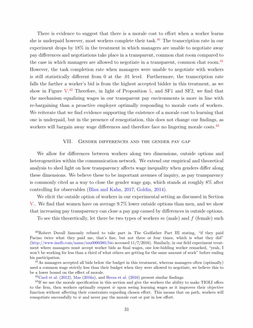
There is evidence to suggest that there is a morale cost to effort when a worker learns

she is underpaid however, most workers complete their task.40 The transcription rate in our

experiment drops by 18% in the treatment in which managers are unable to negotiate away

pay differences and negotiations take place in a transparent, common chat room compared to

the case in which managers are allowed to negotiate in a transparent, common chat room.41

However, the task completion rate when managers were unable to negotiate with workers

is still statistically different from 0 at the .01 level. Furthermore, the transcription rate

falls the farther a worker’s bid is from the highest accepted bidder in this treatment, as we

show in Figure V.42 Therefore, in light of Proposition 5, and SF1 and SF2, we find that

the mechanism equalizing wages in our transparent pay environments is more in line with

re-bargaining than a proactive employer optimally responding to morale costs of workers.

We reiterate that we find evidence supporting the existence of a morale cost to learning that

one is underpaid, but in the presence of renegotiation, this does not change our findings, as

workers will bargain away wage differences and therefore face no lingering morale costs.43

VII. Gender differences and the gender pay gap

We allow for differences between workers along two dimensions, outside options and

heterogeneities within the communication network. We extend our empirical and theoretical

analysis to shed light on how transparency affects wage inequality when genders differ along

these dimensions. We believe these to be important avenues of inquiry, as pay transparency

is commonly cited as a way to close the gender wage gap, which stands at roughly 8% after

controlling for observables (Blau and Kahn, 2017; Goldin, 2014).

We elicit the outside option of workers in our experimental setting as discussed in Section

V.. We find that women have on average 9.7% lower outside options than men, and we show

that increasing pay transparency can close a pay gap caused by differences in outside options.

To see this theoretically, let there be two types of workers m (male) and f (female) such

40Robert Duvall famously refused to take part in The Godfather Part III stating, “if they paidPacino twice what they paid me, that’s fine, but not three or four times, which is what they did”(http://www.imdb.com/name/nm0000380/bio accessed 11/7/2016). Similarly, in our field experiment treat-ment where managers must accept worker bids as final wages, one low-bidding worker remarked, “yeah, Iwon’t be working for less than a third of what others are getting for the same amount of work” before endinghis participation.

41As managers accepted all bids below the budget in this treatment, whereas managers often (optimally)used a common wage strictly less than their budget when they were allowed to negotiate, we believe this tobe a lower bound on the effect of morale.

42Card et al. (2012), Mas (2016a), and Breza et al. (2016) present similar findings.43If we use the morale specification in this section and give the workers the ability to make TIOLI offers

to the firm, then workers optimally request w upon seeing learning wages as it improves their objectivefunction without affecting their constraints regarding chosen effort. This means that on path, workers willrenegotiate successfully to w and never pay the morale cost or put in low effort.

31

that qGm(x) + (1 − q)Gf (x) = G(x) for all x ∈ [0, 1], where Gm(x) and Gf (x) are both

atomless distributions and q ∈ [0, 1] is the proportion of men in the market. The first, and

simplest result, is an application of Theorem 1. Similarly to above, we denote the average

equilibrium lifetime earnings of an employed worker of type ` ∈ {m, f} as T (Λ, v, θi, `).

Corollary 3. If Gm(·) first-order stochastically dominates Gf (·) thenEGf [T (Λ,v,θi,f)]

EGm [T (Λ,v,θi,m)]con-

verges monotonically to 1 as Λ converges to 1 for all v.

In words, this result says that the average earnings of employed women is rising relative

to the average earnings of employed men as transparency increases, and reaching full trans-

parency completely equalizes earnings. The proof of this result follows from Theorem 1.

When Gm(·) first-order stochastically dominates Gf (·), it is possible to pair up every f type

worker with an m type worker with higher outside option. Formally, let µ : [0, 1] → [0, 1]

define for each f type worker i an m type worker j such that θj ≥ θi and µ(θi) 6= µ(θi′ ) for

any i 6= i′. We know by Theorem 1 that T (Λ,v,θi)

T (Λ,v,θj)converges monotonically to 1 in Λ, which

implies that the average income of each worker type also converges monotonically to 1 in Λ.

However, if transparency relies on word-of-mouth, and co-worker networks are dominated

by one gender or the other, permitting communication exacerbates the gender pay gap.

Empirically, we find evidence that network effects heavily mediate the impact of partial

transparency, or open communication, on the gender pay gap. First, we find that men

receive bonuses more often than women on average when workers are co-located, and not

when they are separated (Table VIII). Second, when the majority of workers at a job are

female, all workers, male and female, receive bonuses less often doing co-located work, while

these composition differences do not affect the outcome when workers are separated. This is

in line with findings of our worker surveys, where men report a higher likelihood of learning

about co-worker pay on the job (Figure VII).

We make simple adjustments to the model to capture these network effects. Let αm >

αf > 0 be the rates at which men and women receive wage information, respectively, and let

q be the proportion of men in the industry. Let the arrival rate of information for a worker

of gender ` ∈ {m, f} be α`qλ. Then

Λ` = α`qλρ+δ+α`qλ

for ` ∈ {m, f} and λ ∈ [0,∞) (10)

Network effects cause the de facto arrival rate of information of men to be greater than

that of women, that is, Λm −Λf ≥ 0 for all λ and all q. We plot Λm −Λf as a function of λ

for arbitrary parameters in Figure VI. Λm − Λf is initially increasing but converges to 0.

Proposition 6. Suppose q > 0. Let λc solve αmαf

= (ρ+δ+αmqλ)2

(ρ+δ+αf qλ)2 . Λm−Λf is strictly increasing

in λ for all λ < λc and strictly decreasing for all λ > λc. As λ→∞, Λm − Λf → 0.

32

Compare the effects of moving from zero transparency to some λ > 0. When λ is rela-

tively low, information transmission between workers happens rarely through word of mouth.

Because men are more likely to speak about wages, they disproportionately benefit from low

levels of transparency compared to women. However, when λ is relatively high, men gain

relatively less compared to women because all workers learn information quickly regardless of

their communication propensity. In extreme cases of transparency in which the firm posts a

price (λ =∞) any communication advantage men have completely disappears as information

arrival is not based on word of mouth transmission.

An important implication of these findings is that intermediate levels of transparency,

or transparency relying on communication between co-workers, may exacerbate pay dis-

crepancies. Advocates of gender equality may reconsider whether pursuing and penalizing

employers that prohibit pay discussions will further their cause.

VIII. Conclusion

Pay transparency has been in the political and popular spotlights, but the equilibrium

effects of making pay more transparent have not received adequate attention. Does it result

in more equal wages for similarly productive workers? Does it lead to higher employment

rates? How does it affect the division of surplus between firms and workers?

Our analysis utilizes a methodologically diverse approach, which we view as a strength

of this paper. Our simple, equilibrium model of pay transparency reveals consequences of

pay transparency that may not initially be apparent, and allow us to further the literature

on this policy. With TaskRabbit administrative data, we have the rare opportunity to

observe an employer’s active decision to adjust pay across different settings where large pay

disparities arise through the bidding process for work. In many ways, this data is truly

ideal: we observe initial and renegotiated wages, there is rich demographic information on

both workers and employers, and we have the ability to view jobs that are not completed.

The field experiment we run on internet workers allows for estimation of unobservables in

TaskRabbit, and verification of our findings in a controlled data setting.

Contract labor and short-term work arrangements are growing due to the increased use

of internet labor platforms.44 Transparency related policy interventions, either at the in-

stitution or government level, depend on the particulars of markets. For example, internet

platforms must decide who makes initial wage offers and whether wages can be different

for different workers on a particular job. Although these interventions may not be imple-

mentable in other markets, our model allows for many generalizations and extensions which

44Katz and Krueger (2016) find that 16% of the US workforce relies on alternative work arrangements astheir primary source of income, a figure which grew by over 50% between 2010 and 2015. Oyer (2016) findsthat 30% of American laborers participate in alternative work arrangements.

33

preserve our main findings. Our experiment specifically addresses one key point by allowing

free-form bargaining between workers and managers, and yields similar findings.

We find, theoretically and empirically, that increasing pay transparency decreases in-

equality and can increase employment. We also find that increasing pay transparency shifts

surplus away from workers and toward their employer. Moreover, intermediate levels of

pay transparency, achieved through a permissive environment to discuss relative pay, can

exacerbate the gender pay gap by virtue of how information spreads.

There may be a direct need for external intervention in order to maintain a desirable

level of transparency. We have shown theoretically that any scheme in which the firm

choose transparency based on private characteristics is unsustainable, as the signal sent to

prospective workers is sufficiently strong to cause unraveling toward full transparency. This

is perhaps the most surprising of our results. Do we observe employers self-selecting high

levels of transparency? If so, in what types of jobs?

We find a move toward transparency among employers on TaskRabbit. We also observe

high levels of pay transparency, instituted by employers fixing a common wage, in many

entry level markets. In our profession, incoming assistant professors (and graduate students)

generally receive common wages with little room for individual negotiation; the most common

response that our (informally) surveyed colleagues reported for rejected attempts at wage

negotiation has been that universities are unwilling to pay an incoming assistant professor

more than her peers. Niederle et al. (2006) find that 94% of gastroenterology program

directors for post-medical school fellowships paid common wages to all doctors and “offers

are not adjusted in response to outside offers and terms are not negotiable.” Recently, many

startups in Silicon Valley are opting to be fully transparenct about pay. One common thread

in these markets is that worker productivity is (at least perceived to be) relatively common

across workers: TaskRabbit is built on unskilled, short-term labor, assistant professors and

medical fellows spend significant time learning on the job, and are often sheltered from

professional responsibilities. An interesting avenue of further research is to understand if

there is more pay transparency in jobs with similar worker productivity.

While it is unfeasible to accurately describe every market in a single paper, we believe

that different formulations of our model may be good approximations of some entry-level

labor markets. Combined with our empirical results, we believe many of our findings on

the equilibrium effects of pay transparency may be worthy of consideration in other labor

markets, the specifics of which we leave for future research.

Entrepreneurial Management Unit, Harvard Business School

Department of Economics, Brown University

34

References

John M. Abowd, Francis Kramarz, and David N. Margolis. High Wage Workers and High WageFirms. Econometrica, 67(2):251–333, 1999. I.A.

George A. Akerlof and Janet L. Yellen. The Fair Wage-Effort Hypothesis and Unemployment. TheQuarterly Journal of Economics, 105(2):255–283, 1990. I.A., VI.

Vladimir Asriyan, William Fuchs, and Brett Green. Information Spillovers in Asset Markets withCorrelated Values. Mimeo, 2016. I.A.

Linda Babcock and Sara Laschever. Women Don’t Ask: Negotiation and the Gender Divide. Prince-ton University Press, 2003. I.A.

Jesper Bagger, Francois Fontaine, Fabien Postel-Vinay, and Jean-Marc Robin. Tenure, Experi-ence, Human Capital, and Wages: A Tractable Equilibrium Search Model of Wage Dynamics.American Economic Review, 104(6):1551–1596, 2014. I.A.

Gordon M. Becker, Morris H. DeGroot, and Jacob Marschak. Measuring Utility by a Single-Response Sequential Method. Behavioral Sciences, 9(3):226–232, 1964. V.A., IV

Truman Bewley. Why Wages Don’t Fall During a Recession. Harvard University Press, 1999. I.A.

Francine D. Blau and Lawrence M. Kahn. The Gender Wage Gap: Extent, Trends, and Explana-tions. Journal of Economic Literature, 55(4):789–865, 2017. 1, I.A., VII.

Francis Bloch and Harl Ryder. Two-Sided Search, Marriages, and Matchmakers. InternationalEconomic Review, 41(1):93–115, 2000. 49

Emily Breza, Supreet Kaur, and Yogita Shamdasani. The Morale Effects of Pay Inequality. Mimeo,2016. I., I.A., VI., 42

Kenneth Burdett and Melvyn G. Coles. Long-Term Partnership Formation: Marriage and Employ-ment. The Economic Journal, 109(456):F307–F334, 1999. 49

Kenneth Burdett and Dale T. Mortensen. Wage Differentials, Employer Size, and Unemployment.International Economic Review, 39(2):257–273, 1998. I.A.

Pierre Cahuc, Fabien Postel-Vinay, and Jean-Marc Robin. Wage Bargaining with On-the-JobSearch: Theory and Evidence. Econometrica, 74(2):323–364, 2006. I.A.

David Card, Alexandre Mas, Enrico Moretti, and Emmanuel Saez. Inequality at Work: The Effectof Peer Salaries on Job Satisfaction. American Economic Review, 102(6):2981–3003, 2012. I.A.,VI., 42

Hector Chade. Matching with Noise and the Acceptance Curse. Journal of Economic Theory, 129(1):81–113, 2006. 49

Gary Charness and Peter Kuhn. Do Co-Workers’ Wages Matter? Theory and Evidence on WageSecrecy, Wage Compression and Effort. Discussion Paper Series, IZA DP No. 1417, 2004. I.A.

Kalyan Chatterjee and William Samuelson. Bargaining under Incomplete Information. OperationsResearch, 31(5):835–851, 1983. I.A., II.D.

35

Alice Chen, Emily Oster, and Heidi Williams. Why is Infant Mortality Higher in the US than inEurope? Mimeo, 2014. 1

Daniel L. Chen, Martin Schonger, and Chris Wickens. oTree-An open-source platform for labora-tory, online, and field experiments. Journal of Behavioral and Experimental Finance, 9:88–97,2016. V.C.

Zoe Cullen and Chiara Farronato. Outsourcing Tasks Online: Matching Supply and Demand onPeer-to-Peer Internet Platforms. Mimeo, August 2016. 28, A.2

Alex Edmans, Xavier Gabaix, Tomasz Sadzik, and Yuliy Sannikov. Dynamic CEO Compensation.Journal of Finance, Forthcoming, 2016. 13

Liran Einav, Chiara Farronato, Jonathan D. Levin, and Neel Sundaresan. Sales Mechanisms inOnline Markets: What Happened to Internet Auctions? Mimeo, 2013. A.2.

Diana Farrell and Fiona Greig. Paychecks, Paydays and the Online Platform Economy. JPMorganChase & Co. Institute, 2016. 5

Robert Frank. Are Workers Paid Their Marginal Products? American Economic Review, 74(4):549–571, 1984. I.A.

William Fuchs, Aniko Ory, and Andrzej Skrzypacz. Transparency and Distressed Sales underAsymmetric Information. Theoretical Economics, 11(3):1103–1144, 2016. I.A.

Xavier Gabaix. Power Laws in Economics and Finance. Annual Review of Economics, 1(1):255–294,2009. 13

Xavier Gabaix. Power Laws in Economics: An Introduction. Journal of Economic Perspectives, 30(1):185–206, 2016.

Claudia Goldin. A Grand Gender Convergence: Its Last Chapter. American Economic Review,104(4):1091–1119, 2014. 1, I.A., VII.

Marina Halac. Relational Contracts and the Value of Relationships. American Economic Review,102(2):750–779, 2012. 50

Robert Hall and Alan Krueger. Evidence on the Incidence of Wage Posting, Wage Bargaining, andOn-the-Job Search. American Economic Journal: Macroeconomics, 4(4):56–67, October 2012.3, 20

Johannes Horner and Nicolas Vieille. Public vs. Private Offers in the Market for Lemons. Econo-metrica, 77(1):29–69, 2009. I.A.

Lisa Kahn and Fabian Lange. Employer Learning, Productivity, and the Earnings Distribution:Evidence from Performance Measures. Review of Economics Studies, 81(4):1575–1613, 2016. 9

Michihiro Kandori, George J. Mailath, and Rafael Robb. Learning, Mutation, and Long RunEquilibria in Games. Econometrica, 61(1):29–56, January 1993. IV.H.

Lawrence D. Katz and David H. Autor. Changes in the Wage Structure and Earnings Inequality.In Orley Ashenfelter and David Card, editors, Handbook of Labor Economics. 1999. 1

36

Lawrence F. Katz and Alan B. Krueger. The Rise and Nature of Alternative Work Arrangementsin the United States, 1995-2015. Mimeo, 2016. 44

Ayca Kaya and Quingmin Liu. Transparency and Price Formation. Theoretical Economics, 10:341–383, 2015. I.A.

Lisa Keister. The One Percent. Annual Review of Sociology, 40:347–367, July 2014. I.A.

Elena Kerzner. Lessons Learned from Creating my TaskRabbit Pricing Strategy.http://www.priceintelligently.com/blog/bid/192053/Lessons-Learned-from-Creating-My-TaskRabbit-Pricing-Strategy, 2013. 33

Kyungmin Kim. Information About Sellers’ Past Behavior in the Market for Lemons. Econometrica,169:365–399, 2017. I.A.

Wolfgang Leininger, Peter B. Linhart, and Roy Radner. Equilibria of the Sealed-Bid Mechanismfor Bargaining with Incomplete Information. Journal of Economic Theory, 48:63–106, 1989. I.A.,11

Vladimir I. Levenshtein. Binary codes capable of correcting deletions, insertions, and reversals.Soviet Physics Doklady, 10(8):707–710, 1966. V.C.

Alexandre Mas. Does Transparency Lead to Pay Compression? Journal of Political Economy,Forthcoming, 2016a. I.A., VI., 42

Alexandre Mas. Does Disclosure affect CEO Pay Setting? Evidence from the Passage of the 1934Securities and Exchange Act. Mimeo, 2016b. I.A.

Claudia Moellers, Hans-Theo Normann, and Christopher M. Snyder. Communication in verticalmarkets: Experimental evidence. International Journal of Industrial Organization, 50:214–258,2017. I.A.

Roger Myerson. Optimal Auction Design. Mathematics of Operations Research, 6:58–73, 1981.III.C., D.1., D.1.

Muriel Niederle and Lise Vesterlund. Do Women Shy Away From Competition? Do Men CompeteToo Much? Quarterly Jounal of Economics, 122(3):1067–1101, 2007. I.A.

Muriel Niederle, Deborah D. Proctor, and Alvin E. Roth. What Will Be Needed for the NewGastroenterology Fellowship Match to Succeed? Gastroenterology, 130:218–224, 2006. VIII.

Chris Nosko and Steven Tadelis. The limits of reputation in platform markets: An empiricalanalysis and field experiment. Working paper, 2015. 24, A.

Paul Oyer. The Independent Workforce in America: The Economics of an Increasingly FlexibleLabor Market. Technical report, 2016. 44

Ricardo Perez-Truglia. The Effects of Income Transparency on Well-Being: Evidence from a NaturalExperiment. Mimeo, 2016. I.A., VI.

Thomas Piketty. Capital in the Twenty-First Century. Harvard University Press, 2014. 1

37

Fabien Postel-Vinay and Jean-Marc Robin. The Distribution of Earnings in an Equilibrium SearchModel with State-Dependent Offers and Counteroffers. International Economic Review, 43(4):989–1016, 2002. I.A.

Fabien Postel-Vinay and Jean-Marc Robin. Equilibrium Wage Dispersion with Worker and Em-ployer Heterogeneity. Econometrica, 70(6):2295–2350, 2006. I.A.

Roy Radner and Andrew Schotter. The Sealed-Bid Mechanism: An Experimental Study. Journalof Economic Theory, 48:179–220, 1989. I.A., II.E.

Alvin E. Roth and Xiaolin Xing. Jumping the Gun: Imperfections and Institutions Related to theTiming of Market Transactions. American Economic Review, 84(4):992–1044, 1994. 32

Emmanuel Saez and Gabriel Zucman. Wealth Inequality in the United States since 1913: Evidencefrom Capitalized Income Tax Data. Mimeo, 2014. 1

Mark A. Satterthwaite and Steven R. Williams. Bilateral Trade with the Sealed Bid k-DoubleAuction: Existence and Efficiency. Journal of Economic Theory, 48:107–133, 1989. I.A., II.D.,II.E.

Jae Song, David J. Price, Fatih Guvenen, Nicholas Bloom, and Till von Wachter. Firming UpInequality. Mimeo, 2016. I.A.

Jean Tirole. From Bottom of the Barrel to Cream of the Crop: Sequential Screening with PositiveSelection. Econometrica, Forthcoming, 2016. 12

Donald M. Topkis. Supermodularity and Complementarity. Princeton University Press, 1998. 2

Joel Watson. Perfect Bayesian Equilibrium: General Definitions and Illustrations. Mimeo, 2016.45

Martin L. Weitzman. The ‘Ratchet Principle’ and Performance Incentives. Bell Journal of Eco-nomics, 11(1):302–308, 1980. II.C.

Steven R. Williams. Efficient Performancy in Two Agent Bargaining. Journal of Economic Theory,41:154–172, 1987. I.A.

38

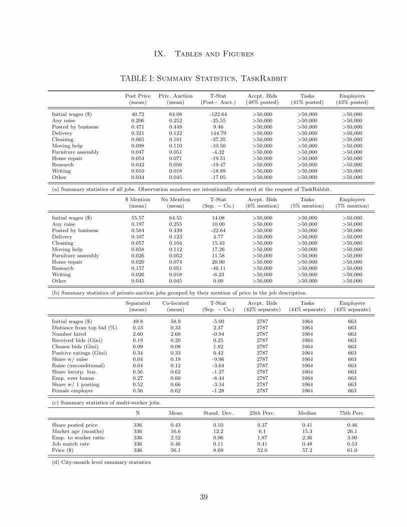
IX. Tables and Figures

TABLE I: Summary Statistics, TaskRabbit

Post Price Priv. Auction T-Stat Accpt. Bids Tasks Employers(mean) (mean) (Post− Auct.) (48% posted) (41% posted) (43% posted)

Initial wages ($) 40.72 64.08 -122.64 >50,000 >50,000 >50,000Any raise 0.206 0.252 -25.55 >50,000 >50,000 >50,000Posted by business 0.471 0.448 9.46 >50,000 >50,000 >50,000Delivery 0.321 0.122 144.79 >50,000 >50,000 >50,000Cleaning 0.065 0.101 -37.35 >50,000 >50,000 >50,000Moving help 0.098 0.110 -10.50 >50,000 >50,000 >50,000Furniture assembly 0.047 0.051 -4.32 >50,000 >50,000 >50,000Home repair 0.054 0.071 -19.51 >50,000 >50,000 >50,000Research 0.042 0.056 -19.47 >50,000 >50,000 >50,000Writing 0.010 0.018 -18.89 >50,000 >50,000 >50,000Other 0.034 0.045 -17.05 >50,000 >50,000 >50,000

(a) Summary statistics of all jobs. Observation numbers are intentionally obscured at the request of TaskRabbit.

$ Mention No Mention T-Stat Accpt. Bids Tasks Employers(mean) (mean) (Sep. − Co.) (6% mention) (5% mention) (7% mention)

Initial wages ($) 55.57 64.55 14.08 >50,000 >50,000 >50,000Any raise 0.197 0.255 10.00 >50,000 >50,000 >50,000Posted by business 0.584 0.439 -22.64 >50,000 >50,000 >50,000Delivery 0.107 0.123 4.77 >50,000 >50,000 >50,000Cleaning 0.057 0.104 15.43 >50,000 >50,000 >50,000Moving help 0.058 0.112 17.26 >50,000 >50,000 >50,000Furniture assembly 0.026 0.052 11.58 >50,000 >50,000 >50,000Home repair 0.020 0.074 20.90 >50,000 >50,000 >50,000Research 0.157 0.051 -46.11 >50,000 >50,000 >50,000Writing 0.026 0.018 -6.23 >50,000 >50,000 >50,000Other 0.045 0.045 0.00 >50,000 >50,000 >50,000

(b) Summary statistics of private-auction jobs grouped by their mention of price in the job description.

Separated Co-located T-Stat Accpt. Bids Tasks Employers(mean) (mean) (Sep. − Co.) (42% separate) (44% separate) (43% separate)

Initial wages ($) 49.8 58.9 -5.00 2787 1064 663Distance from top bid (%) 0.43 0.33 2.37 2787 1064 663Number hired 2.60 2.69 -0.94 2787 1064 663Received bids (Gini) 0.19 0.20 0.25 2787 1064 663Chosen bids (Gini) 0.09 0.08 1.82 2787 1064 663Positive ratings (Gini) 0.34 0.33 0.42 2787 1064 663Share w/ raise 0.04 0.19 -9.96 2787 1064 663Raise (unconditional) 0.04 0.12 -3.64 2787 1064 663Share incorp. bus. 0.56 0.62 -1.27 2787 1064 663Emp. ever bonus 0.27 0.60 -8.44 2787 1064 663Share w/ 1 posting 0.52 0.66 -3.34 2787 1064 663Female employer 0.56 0.62 -1.28 2787 1064 663

(c) Summary statistics of multi-worker jobs.

N Mean Stand. Dev. 25th Perc. Median 75th Perc.

Share posted price 336 0.43 0.10 0.37 0.41 0.46Market age (months) 336 16.6 12.2 6.1 15.3 26.1Emp. to worker ratio 336 2.52 0.96 1.87 2.36 3.00Job match rate 336 0.46 0.11 0.41 0.48 0.53Price ($) 336 56.1 8.69 52.0 57.2 61.0

(d) City-month level summary statistics

39

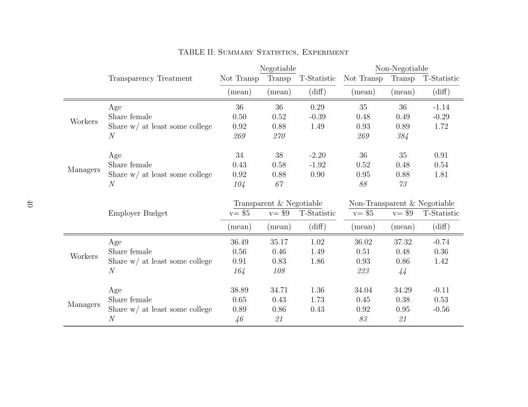
TABLE II: Summary Statistics, Experiment

Negotiable Non-NegotiableTransparency Treatment Not Transp Transp T-Statistic Not Transp Transp T-Statistic

(mean) (mean) (diff) (mean) (mean) (diff)

Workers

Age 36 36 0.29 35 36 -1.14Share female 0.50 0.52 -0.39 0.48 0.49 -0.29Share w/ at least some college 0.92 0.88 1.49 0.93 0.89 1.72N 269 270 269 384

Managers

Age 34 38 -2.20 36 35 0.91Share female 0.43 0.58 -1.92 0.52 0.48 0.54Share w/ at least some college 0.92 0.88 0.90 0.95 0.88 1.81N 104 67 88 73

Transparent & Negotiable Non-Transparent & NegotiableEmployer Budget v= $5 v= $9 T-Statistic v= $5 v= $9 T-Statistic

(mean) (mean) (diff) (mean) (mean) (diff)

Workers

Age 36.49 35.17 1.02 36.02 37.32 -0.74Share female 0.56 0.46 1.49 0.51 0.48 0.36Share w/ at least some college 0.91 0.83 1.86 0.93 0.86 1.42N 164 108 223 44

Managers

Age 38.89 34.71 1.36 34.04 34.29 -0.11Share female 0.65 0.43 1.73 0.45 0.38 0.53Share w/ at least some college 0.89 0.86 0.43 0.92 0.95 -0.56N 46 21 83 21

40

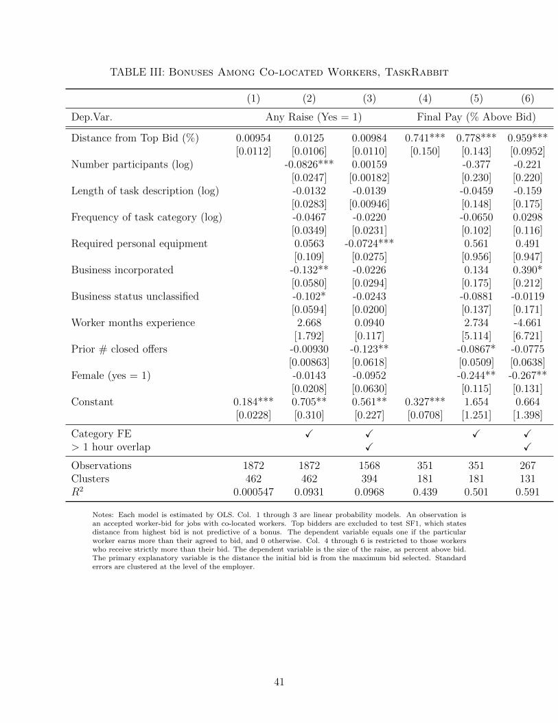
TABLE III: Bonuses Among Co-located Workers, TaskRabbit

(1) (2) (3) (4) (5) (6)

Dep.Var. Any Raise (Yes = 1) Final Pay (% Above Bid)

Distance from Top Bid (%) 0.00954 0.0125 0.00984 0.741*** 0.778*** 0.959***[0.0112] [0.0106] [0.0110] [0.150] [0.143] [0.0952]

Number participants (log) -0.0826*** 0.00159 -0.377 -0.221[0.0247] [0.00182] [0.230] [0.220]

Length of task description (log) -0.0132 -0.0139 -0.0459 -0.159[0.0283] [0.00946] [0.148] [0.175]

Frequency of task category (log) -0.0467 -0.0220 -0.0650 0.0298[0.0349] [0.0231] [0.102] [0.116]

Required personal equipment 0.0563 -0.0724*** 0.561 0.491[0.109] [0.0275] [0.956] [0.947]

Business incorporated -0.132** -0.0226 0.134 0.390*[0.0580] [0.0294] [0.175] [0.212]

Business status unclassified -0.102* -0.0243 -0.0881 -0.0119[0.0594] [0.0200] [0.137] [0.171]

Worker months experience 2.668 0.0940 2.734 -4.661[1.792] [0.117] [5.114] [6.721]

Prior # closed offers -0.00930 -0.123** -0.0867* -0.0775[0.00863] [0.0618] [0.0509] [0.0638]

Female (yes = 1) -0.0143 -0.0952 -0.244** -0.267**[0.0208] [0.0630] [0.115] [0.131]

Constant 0.184*** 0.705** 0.561** 0.327*** 1.654 0.664[0.0228] [0.310] [0.227] [0.0708] [1.251] [1.398]

Category FE X X X X> 1 hour overlap X X

Observations 1872 1872 1568 351 351 267Clusters 462 462 394 181 181 131R2 0.000547 0.0931 0.0968 0.439 0.501 0.591

Notes: Each model is estimated by OLS. Col. 1 through 3 are linear probability models. An observation isan accepted worker-bid for jobs with co-located workers. Top bidders are excluded to test SF1, which statesdistance from highest bid is not predictive of a bonus. The dependent variable equals one if the particularworker earns more than their agreed to bid, and 0 otherwise. Col. 4 through 6 is restricted to those workerswho receive strictly more than their bid. The dependent variable is the size of the raise, as percent above bid.The primary explanatory variable is the distance the initial bid is from the maximum bid selected. Standarderrors are clustered at the level of the employer.

41

TABLE IV: Dispersion in Final Wages and Worker Surplus

TaskRabbit Experimental Evidence

(1) (2) (3) (4) (5) (6) (7) (8) (9)

Dep. Var. Final Pay (Gini) Final Pay (Gini) Hourly Wage (Gini) Worker Surplus (Gini)

Transp. -0.0463** -0.0648*** -0.111*** Transp. -0.0232*** -0.0215*** 0.0282 0.0233 0.243** 0.311**(Co-loc.) [0.0222] [0.0220] [0.0286] (Co-loc.) [0.00707] [0.00802] [0.0363] [0.0376] [0.118] [0.141]Constant 0.126*** 0.141*** 0.217** Constant 0.0232*** 0.114 0.144*** 0.0933 0.115** -0.164

[0.0219] [0.0220] [0.0898] [0.00707] [0.0935] [0.0219] [0.215] [0.0454] [0.449]Category FE X X Mgr. Char. X X XEmployer FE X

Mean D.V. 0.0829 0.0829 0.0829 0.0147 0.0147 0.154 0.154 0.204 0.204Obs. 1046 1046 1046 Obs. 74 74 74 74 74 74R2 0.0180 0.0971 0.810 R2 0.0794 0.171 0.00831 0.122 0.0729 0.146

Notes: Each model is estimated by OLS. An observation is a multi-worker local task. Standard errors are clustered at the employer level. The dependentvariable in Col. 1 - 3 is the dispersion of the final pay in a TaskRabbit multi-worker job measured by the Gini Coefficient. Col. 4 -9 present experimentalevidence. The dependent variable Col. 4-5 is the dispersion in final pay, in Col. 6 and 7 dispersion in hourly wages, and in Col. 8 and 9 dispersion in workersurplus, which we measured by subtracting employees’ minimum willingness to accept the job (elicited using an incentive compatible method similar to that ofBecker et al. (1964)) from the price paid. Manager characteristics in the experimental setting include gender, age, age squared managerial experience, and yearsof formal education.

42

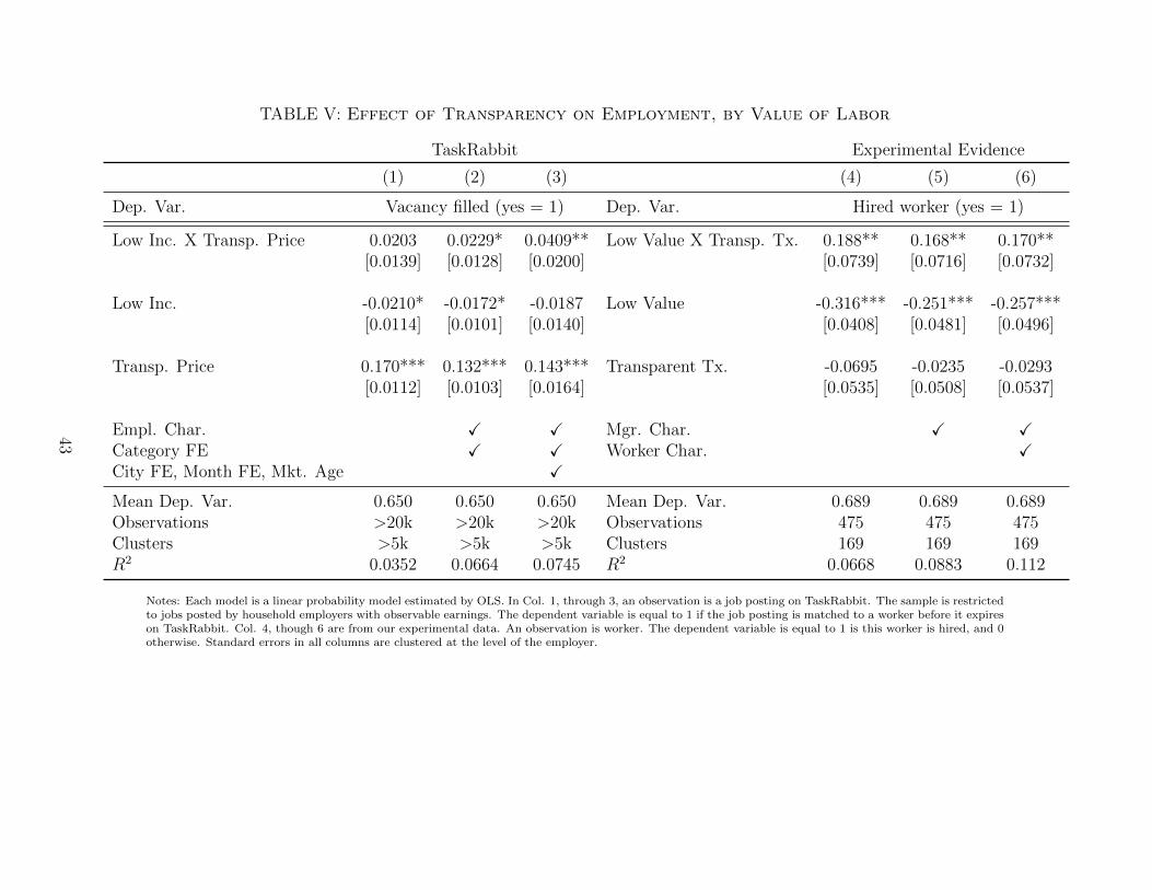
TABLE V: Effect of Transparency on Employment, by Value of Labor

TaskRabbit Experimental Evidence

(1) (2) (3) (4) (5) (6)

Dep. Var. Vacancy filled (yes = 1) Dep. Var. Hired worker (yes = 1)

Low Inc. X Transp. Price 0.0203 0.0229* 0.0409** Low Value X Transp. Tx. 0.188** 0.168** 0.170**[0.0139] [0.0128] [0.0200] [0.0739] [0.0716] [0.0732]

Low Inc. -0.0210* -0.0172* -0.0187 Low Value -0.316*** -0.251*** -0.257***[0.0114] [0.0101] [0.0140] [0.0408] [0.0481] [0.0496]

Transp. Price 0.170*** 0.132*** 0.143*** Transparent Tx. -0.0695 -0.0235 -0.0293[0.0112] [0.0103] [0.0164] [0.0535] [0.0508] [0.0537]

Empl. Char. X X Mgr. Char. X XCategory FE X X Worker Char. XCity FE, Month FE, Mkt. Age X

Mean Dep. Var. 0.650 0.650 0.650 Mean Dep. Var. 0.689 0.689 0.689Observations >20k >20k >20k Observations 475 475 475Clusters >5k >5k >5k Clusters 169 169 169R2 0.0352 0.0664 0.0745 R2 0.0668 0.0883 0.112

Notes: Each model is a linear probability model estimated by OLS. In Col. 1, through 3, an observation is a job posting on TaskRabbit. The sample is restrictedto jobs posted by household employers with observable earnings. The dependent variable is equal to 1 if the job posting is matched to a worker before it expireson TaskRabbit. Col. 4, though 6 are from our experimental data. An observation is worker. The dependent variable is equal to 1 is this worker is hired, and 0otherwise. Standard errors in all columns are clustered at the level of the employer.

43

TABLE VI: Endogenous Selection of Transparent Pricing, TaskRabbit

(1) (2) (3) (4) (5) (6)

Dep. Var. Choose Transparent Posted Price (yes =1)

Low Income Employer 0.0622** 0.0641** 0.0456* 0.0448* 0.0452* 0.0579*[0.0269] [0.0272] [0.0270] [0.0269] [0.0270] [0.0329]

Employer Age -0.00147*** -0.000511 -0.000524 -0.000536 -0.00109[0.000557] [0.000524] [0.000527] [0.000528] [0.000672]

Empl. Gender (Fem = 1) -0.0130 -0.00901 -0.00926 -0.00921 -0.0144[0.0148] [0.0130] [0.0129] [0.0129] [0.0163]

Age of Marketplace -0.000895 -0.0000381[0.000592] [0.000714]

Constant 0.323*** 0.390*** 0.221*** 0.225*** 0.256*** 0.215***[0.0259] [0.0359] [0.0538] [0.0573] [0.0602] [0.0720]

Category FE X X X XMetro FE X X XExclude 1st time users X

Mean Dep. Var. 0.423 0.423 0.423 0.423 0.423 0.423Observations >20k >20k >20k >20k >20k >20kClusters >5k >5k >5k >5k >5k >5kR2 0.000432 0.00177 0.100 0.101 0.102 0.112

Notes: All columns are linear probability models estimated by OLS. An observation is a job post on TaskRabbit.The sample is restricted to jobs posted by household employers with observable earnings. The dependent variableis equal to 1 if the employer chose to post the job using a transparent (public) posted price, and 0 if the employerchooses to accept private bids. The primary explanatory variable, low income, is an indicator equal to 1 if theemployer earns less than the median earning household in each city, approximately $150k annually. Standarderrors are clustered at the level of the employer.

44

TABLE VII: Share of Jobs with Fully Transparent Posted Price, TaskRabbit

(1) (2) (3) (4)

Dep. Var. Proportion of Jobs with Posted Price

Market age (months) 0.0109∗∗∗ 0.00894∗ 0.0119∗∗∗ 0.0102∗∗

[0.0000198] [0.00426] [0.00103] [0.00383]

City FE X X X XCalendar months FE X X X XNumber of posts per month (thousands) X XShare of jobs in each category X X

Observations 417 417 417 417Clusters 19 19 19 19R2 0.668 0.731 0.717 0.734

Notes: Each model is estimated by OLS. An observation is a city-month in TaskRabbit. The dependent variableis the proportion of tasks that use the transparent posted price scheme. Standard errors are clustered at thecity level.

45

TABLE VIII: Gender gap in likelihood of raise rises in co-located, partiallytransparent jobs, TaskRabbit

(1) (2) (3) (4) (5) (6)

Dep.Var. Any Raise (Yes = 1) Final Pay (% Above Bid)

Together 0.183*** 0.164*** 0.162*** 0.159 0.113 0.216[0.0262] [0.0232] [0.0239] [0.163] [0.247] [0.366]

X Female (yes = 1) -0.0905*** -0.0670*** -0.0728*** 0.155 0.314 0.367[0.0263] [0.0239] [0.0258] [0.220] [0.297] [0.436]

Female (yes = 1) 0.00859 0.0423*** 0.0430*** -0.0599 -0.191 -0.206[0.0153] [0.0164] [0.0152] [0.158] [0.220] [0.349]

Exp. on platform (months) 0.00192 0.000912 -0.000453 -0.00261[0.00131] [0.00130] [0.00547] [0.00700]

Prior # closed offers -0.00848 -0.0104 -0.0777 -0.0662[0.00654] [0.00697] [0.0548] [0.0718]

No. workers (log) -0.0780*** -0.0646*** -0.288 -0.352[0.0190] [0.0211] [0.282] [0.336]

Length of job post (log) -0.0100 -0.0145 0.0169 0.0300[0.0218] [0.0226] [0.198] [0.254]

Freq. of task category (log) -0.0488 -0.0266 -0.219 -0.159[0.0336] [0.0207] [0.153] [0.145]

Required equipment 0.0405 0.0683 0.595 0.501[0.0926] [0.0981] [0.894] [0.901]

Business incorporated -0.100** -0.0911* 0.116 0.168[0.0459] [0.0478] [0.198] [0.264]

Business status unclassified -0.0885* -0.0846* -0.190 -0.202[0.0458] [0.0478] [0.179] [0.240]

Constant 0.0408*** 0.518* 0.345* 0.415*** 2.839* 2.046[0.0117] [0.289] [0.206] [0.142] [1.632] [1.617]

Category FE X X X X> 1 hour overlap X X

Observations 2644 2644 385 385 288 288Clusters 605 605 195 195 139 139R2 0.0419 0.104 0.110 0.00405 0.0617 0.0522

Notes: Each model is estimated by OLS. Standard errors are clustered at the level of the job. An observationis a worker-bid in a co-located, multi-worker job on TaskRabbit using a private auction. Col. 1 through 3are linear probability models. The dependent variable equals 1 if the particular worker earns more than theirinitial bid, and 0 otherwise. Col. 4 though 6 are restricted to those workers who receive more than theirbid. The dependent variable is the size of the raise, as percent above bid. The primary explanatory variableis an indicator for whether the job entails co-location of workers (a measure of partial transparency) and itsinteraction with the gender of the worker.

46

TABLE IX: Higher Profits Under Transparency, TaskRabbit

TaskRabbit Experimental Evidence

(1) (2) (3) (4) (5) (6)

All Bids Winners’ Pay Winners’ Pay Wages Employed Profits(log) (log) (log hourly wages) (log) (share) (arc sinh)

Transparency -0.0959*** -0.136*** -0.0778*** Full Transparency -0.257** 0.113* 0.617***[0.0136] [0.0142] [0.0281] [0.0958] [0.0641] [0.224]

Exp. on platform (days) 0.378** 0.493*** 1.048*** High School* 0.327** -0.565*** -0.746[0.175] [0.123] [0.393] [0.142] [0.116] [0.530]

# reviews in category -0.991*** -0.512*** 1.921*** Some College 0.220* -0.417*** -1.349***[0.0859] [0.172] [0.308] [0.123] [0.0801] [0.259]

# ratings overall 1.656*** 1.694*** 0.361 College 0.550*** -0.360*** -0.890***[0.0546] [0.123] [0.400] [0.107] [0.0750] [0.271]

Mean rating in category 0.0476*** 0.0792*** 0.0230 Post Graduate 0.342** -0.309*** -1.355***[0.00733] [0.0199] [0.0363] [0.129] [0.0838] [0.309]

Mean rating overall -0.00385 -0.0168 -0.0591 Age 0.0679 -0.00707 0.0481[0.0114] [0.0330] [0.0796] [0.0460] [0.0158] [0.0685]

Age Sqr. -0.000767 0.0000934 -0.000298Category FE X X X [0.000539] [0.000180] [0.000832]Worker FE X X X Female 0.0382 -0.0791 -0.454**Polynomial terms X X X [0.104] [0.0641] [0.209]

Mean Dep. Var. 3.37 3.69 3.02 Mean Dep. Var. 2.883 0.589 0.666Observations >100k >100k 19827 Observations 47 90 90R2 0.277 0.381 0.607 R2 0.380 0.132 0.236

Notes: Each model is estimated by OLS. An observation is a worker-bid on TaskRabbit. The dependent variable in Col. 1 is the log bid received, and finalpay in Col. 2 and 3. In Col. 3 we restrict the sample to jobs that solicit hourly wage bids rather than piece rate. Transparency in TaskRabbit refers to anindicator equal to one if there is any mention of price in the job post. Only job posts that accept private bids are included in these regressions. Platform tenureis measured in days. Polynomial terms includes the square of all covariates. In Col. 4-6, our sample is from our experimental setting. An observation is a worker(Col. 4) or manager (Col. 5-6) in our experiment. The dependent variables are log wages, share of participants hired to complete the transcription, and inversehyperbolic sine of profits a manager earns. Education* is a categorical variable with reference category, some high school. Covariates refer to the worker in Col.4, and the manager in Col. 5-6. Robust standard errors are in square brackets.

47

Figure III: Effects of increasing Λ on worker and firm strategies

(a)

00 θi w∗i 1

w

1

(b)

00 θi 1

w

2

(c)

00 θi 1

w

4

(d)

00 θi w∗′i

1

w

5

Notes: (a) By Equation 5, worker i picks an initial wage offer w∗i that equalizes w−θi1−Λ

(the black, upward sloping

line) and1−F (w)

f(w)(the orange, downward sloping line). (b) The demand effect of increasing Λ from 0 to 3

4

reduces w for each v, shifting1−F (w)

f(w)to the left. (c) The supply effect of increasing Λ from 0 to 3

4increases

the slope of the function w−θi1−Λ

. (d) The supply and income effects combine to reduce the initial wage offer

of worker i to w∗′

i when Λ increases.

48

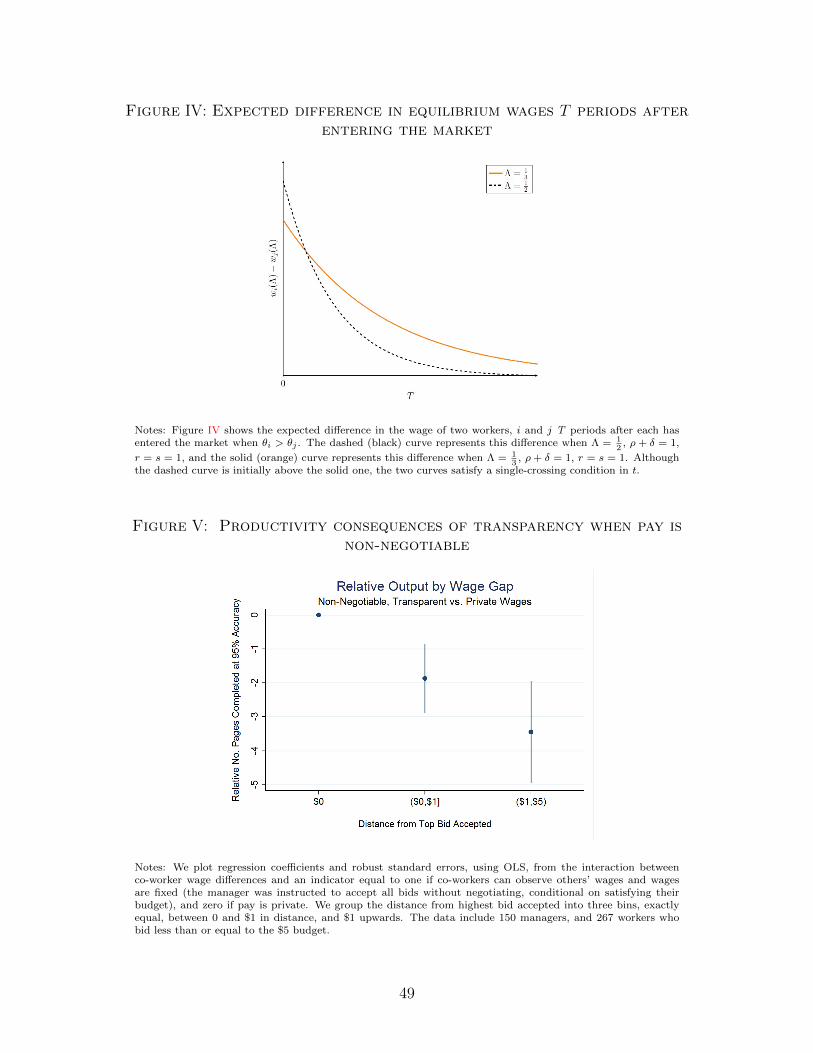
Figure IV: Expected difference in equilibrium wages T periods afterentering the market

Notes: Figure IV shows the expected difference in the wage of two workers, i and j T periods after each hasentered the market when θi > θj . The dashed (black) curve represents this difference when Λ = 1

2, ρ+ δ = 1,

r = s = 1, and the solid (orange) curve represents this difference when Λ = 13

, ρ+ δ = 1, r = s = 1. Althoughthe dashed curve is initially above the solid one, the two curves satisfy a single-crossing condition in t.

Figure V: Productivity consequences of transparency when pay isnon-negotiable

Notes: We plot regression coefficients and robust standard errors, using OLS, from the interaction betweenco-worker wage differences and an indicator equal to one if co-workers can observe others’ wages and wagesare fixed (the manager was instructed to accept all bids without negotiating, conditional on satisfying theirbudget), and zero if pay is private. We group the distance from highest bid accepted into three bins, exactlyequal, between 0 and $1 in distance, and $1 upwards. The data include 150 managers, and 267 workers whobid less than or equal to the $5 budget.

49

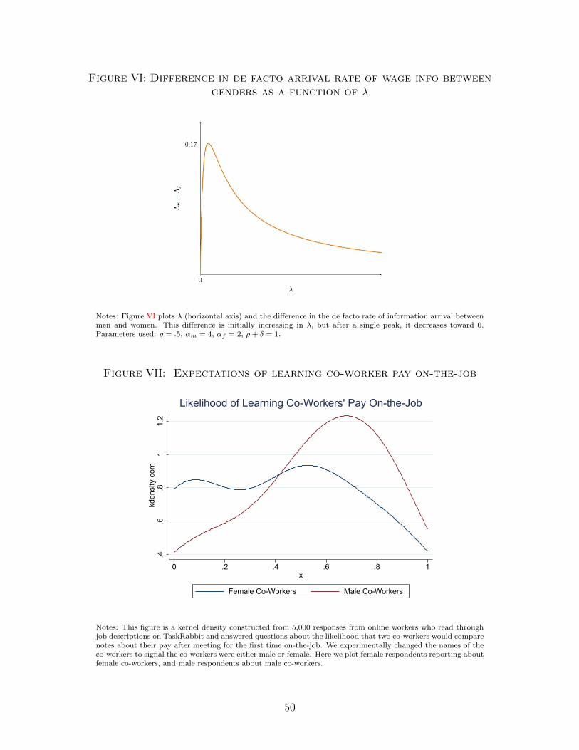
Figure VI: Difference in de facto arrival rate of wage info betweengenders as a function of λ

Notes: Figure VI plots λ (horizontal axis) and the difference in the de facto rate of information arrival betweenmen and women. This difference is initially increasing in λ, but after a single peak, it decreases toward 0.Parameters used: q = .5, αm = 4, αf = 2, ρ+ δ = 1.

Figure VII: Expectations of learning co-worker pay on-the-job

.4.6

.81

1.2

kden

sity

com

0 .2 .4 .6 .8 1x

Female Co-Workers Male Co-Workers

Likelihood of Learning Co-Workers' Pay On-the-Job

Notes: This figure is a kernel density constructed from 5,000 responses from online workers who read throughjob descriptions on TaskRabbit and answered questions about the likelihood that two co-workers would comparenotes about their pay after meeting for the first time on-the-job. We experimentally changed the names of theco-workers to signal the co-workers were either male or female. Here we plot female respondents reporting aboutfemale co-workers, and male respondents about male co-workers.

50

ONLINE APPENDIX: FOR ELECTRONIC

PUBLICATION ONLY

A. Tests of alternative explanations

In this section we assess mechanisms other than communication about pay per se thatcould explain the distinct wage setting behavior we observe when workers are co-located.Chief among them are productivity spillovers, either observed or perceived. Under a pay-for-performance framework, an employer may assign more compressed wages to workers iftheir performance converges or if the employer cannot attribute the output to individualworkers.

Perceived productivity differences, as the explanation for the wage compression we ob-serve, requires that (1) employers compensate workers according to their on-the-job assessedperformance and (2) assessed performance of co-workers is less dispersed when workers aretogether.

We find evidence that a component of pay reflects on-the-job performance using a measureof performance constructed from back-end administrative data (effective percent positivescore (EPP), detailed in Nosko and Tadelis (2015)). However, we do not find empiricalevidence to support (2). Performance measures are no more dispersed or compressed whenworkers are co-located. In Table A.3, the dependent variable is the dispersion of ratingsgiven to workers at the conclusion of the job, expressed as the Gini coefficient. An indicatorvariable of whether these workers operate together or separately proves uninformative aboutthe final dispersion of ex-post ratings. Since we find no evidence that employer evaluations(or ex-post ratings) converge among workers when they are together, it is unlikely thatproductivity drives the wage compression we observe.

More generally, there is a weak relationship between bids and productivity. Our life-time performance measure for workers, which employers can not fully observe at the time ofhire, are not reflected in offers and accepted bids (Table A.2 Col.1). When we can observeproductivity directly in our field experiment we find a small and insignificant relationshipbetween output and bids. A high productivity type might have both lower costs of effortand higher opportunity costs. While our measures of productivity on TaskRabbit are strongpredictors of real outcomes (return customers) they do not explain much of the variance inmarket wage, so any systematic pattern of spillovers does not necessarily raise the perfor-mance of the low bidder or the pay of the low bidder per se. In other words, a model ofpositive spillovers where the most productive worker pulls up the performance of the leastproductive worker, would not imply that the lowest bidder improves performance per se andhence compressed performance pay.

We also do not find evidence of compression resulting from employer preferences forequity among workers hired to do the same tasks. Among workers assessed as equivalentlyproductive by the same employer, those hired to work concurrently in one location earn moreequal pay than those hired by the same employer to work in physically separated locations.Hence, an intrinsic preference for pay equity is unlikely to be the driver of wage compression.

1

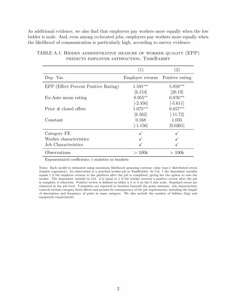
As additional evidence, we also find that employers pay workers more equally when the lowbidder is male. And, even among co-located jobs, employers pay workers more equally whenthe likelihood of communication is particularly high, according to survey evidence.

TABLE A.1: Hidden administrative measure of worker quality (EPP)predicts employer satisfaction, TaskRabbit

(1) (2)

Dep. Var. Employer returns Positive rating

EPP (Effect Percent Positive Rating) 1.591∗∗∗ 5.858∗∗∗

[6.154] [20.19]Ex-Ante mean rating 0.955∗∗ 0.876∗∗∗

[-2.456] [-5.611]Prior # closed offers 1.075∗∗∗ 0.857∗∗∗

[6.562] [-11.72]Constant 0.168 1.035

[-1.156] [0.0261]

Category FE X XWorker characteristics X XJob Characteristics X X

Observations > 100k > 100k

Exponentiated coefficients; t statistics in brackets

Notes: Each model is estimated using maximum likelihood assuming extreme value type-1 distributed errors(logistic regression). An observation is a matched worker-job in TaskRabbit. In Col. 1 the dependent variableequals 1 if the employer returns to the platform after the job is completed, giving her the option to rate theworker. The dependent variable in Col. 2 is equal to 1 if the worker receives a positive review after the jobis complete, 0 otherwise. Positive review is defined as either a 4 or 5 on the 5 star scale. Standard errors areclustered at the job level. T-statistics are reported in brackets beneath the point estimate. Job characteristiccontrols include category fixed effects and proxies for transparency of the job requirements, including the lengthof description and frequency of posts in same category. We also include the number of bidders (log) andequipment requirements.

2

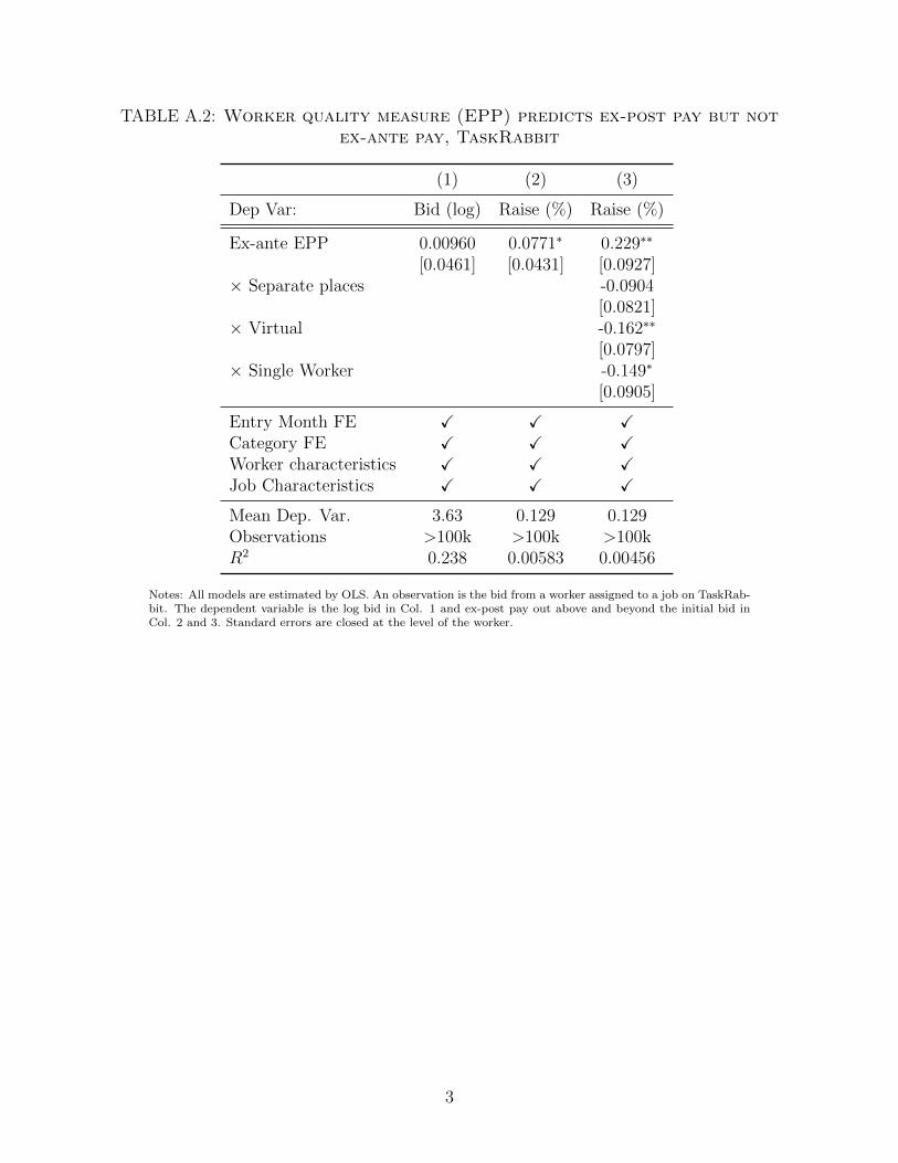
TABLE A.2: Worker quality measure (EPP) predicts ex-post pay but notex-ante pay, TaskRabbit

(1) (2) (3)

Dep Var: Bid (log) Raise (%) Raise (%)

Ex-ante EPP 0.00960 0.0771∗ 0.229∗∗

[0.0461] [0.0431] [0.0927]× Separate places -0.0904

[0.0821]× Virtual -0.162∗∗

[0.0797]× Single Worker -0.149∗

[0.0905]

Entry Month FE X X XCategory FE X X XWorker characteristics X X XJob Characteristics X X X

Mean Dep. Var. 3.63 0.129 0.129Observations >100k >100k >100kR2 0.238 0.00583 0.00456

Notes: All models are estimated by OLS. An observation is the bid from a worker assigned to a job on TaskRab-bit. The dependent variable is the log bid in Col. 1 and ex-post pay out above and beyond the initial bid inCol. 2 and 3. Standard errors are closed at the level of the worker.

3

TABLE A.3: Dispersion in Perceived Worker Performance, TaskRabbit

(1) (2) (3)

Dep. Var. Worker Performance Ratings (Gini)

Transp. (Co-loc.) -0.00946 -0.00788 0.0294[0.0235] [0.0204] [0.0542]

Constant 0.406*** 0.675*** 0.406***[0.0201] [0.0637] [0.0921]

Category FE X XEmployer FE X

Mean Dep. Var. 0.435 0.435 0.435Observations 1064 1064 1064Clusters 618 618 618R2 0.000260 0.0796 0.725

Notes: Each model is estimated by OLS. An observation is a multi-worker job in TaskRabbit. Standard errorsare clustered at the employer level. The dependent variable is the dispersion in ratings received after work iscompleted, measured by a Gini coefficient.

A.1. Strategic bidding, worker selection, and unanticipated transparency

For a causal interpretation of the effect of co-location on ex-post relative wages in ourTaskRabbit population, we must show the composition of workers is similar across settingsas are worker’ bids. Prima facie evidence supports these assumptions. Multi-worker taskscomprise fewer than 5 percent of posted jobs and workers are often unaware that more thanone vacancy exists even when it does. Additionally, employers rarely have more offers thatthe number necessary to complete a multi-worker job. Here we offer more empirical tests.

We observe that the mean and dispersion of bids received are similar across job settings.We also find that dispersion in selected offers is no different across setting. Irrespective ofwork setting, employers select bids that exhibit roughly one-third of the dispersion of offersreceived.

As another test of our assumptions that workers, in this particular environment, do notbid strategically in anticipation of learning pay, we split a sample of co-located jobs bywhether or not the employer explicitly mentions that the tasks require multiple people (eg.“we need two people to load boxes” vs “load boxes between 12-2p”). 54% of job postingsfor co-located, multi-worker jobs do not reveal to workers that there are other workers onthe job. In these jobs, workers are unlikely to be able to anticipate transparency. We findalmost all worker characteristics are not statistically different (Table A.4). Table A.5 showswe cannot reject that bids are similar among those bidding on postings that do and do notreveal multiple workers are required. However, we may not have the specification or powerrequired to detect many forms of strategic bidding.

4

TABLE A.4: Comparision of job characteristic and worker characteristicsfor job postings that do or do not mention multiple workers required,

TaskRabbit

Mention No Mention Difference(Mean) (Mean) (T-Statistic)

Job Characteristics

No. workers req. (log) 0.82 0.84 -0.82Frequency of job post (log) 0.39 0.36 0.18Length of description (log) 3.52 3.45 1.51Total postings in job category (log) 10.0 10.0 -0.56Business (yes = 1) 2.10 1.94 0.55Female employer 0.66 0.53 2.98

Worker Characteristics

Months on platform 9.5 8.1 1.67Mean star rating 4.49 4.19 1.82Effective percent positive (EPP) 0.74 0.75 -0.28Number of completed jobs 2.93 2.58 2.57

Share of postings 0.54 0.46

Notes: Comparison of mean characteristics across jobs that do and do not mention in the job description thatmultiple workers will be carrying out the job in tandem.

5

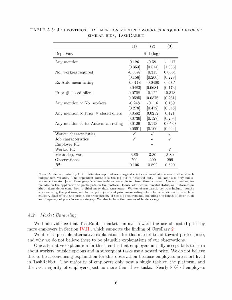
TABLE A.5: Job postings that mention multiple workers required receivesimilar bids, TaskRabbit

(1) (2) (3)

Dep. Var. Bid (log)

Any mention 0.126 -0.581 -1.117[0.353] [0.514] [1.035]

No. workers required -0.0597 0.313 0.0864[0.156] [0.260] [0.228]

Ex-Ante mean rating -0.0118 -0.0480 0.304∗

[0.0483] [0.0681] [0.173]Prior # closed offers 0.0708 0.122 -0.318

[0.0595] [0.0876] [0.231]Any mention × No. workers -0.248 -0.116 0.169

[0.278] [0.472] [0.548]Any mention × Prior # closed offers 0.0582 0.0252 0.121

[0.0736] [0.127] [0.203]Any mention × Ex-Ante mean rating 0.0129 0.113 0.0539

[0.0691] [0.100] [0.244]

Worker characteristics X X XJob characteristics X X XEmployer FE XWorker FE XMean dep. var. 3.80 3.80 3.80Observations 299 299 299R2 0.106 0.892 0.890

Notes: Model estimated by OLS. Estimates reported are marginal effects evaluated at the mean value of eachindependent variable. The dependent variable is the log bid of accepted bids. The sample is only multi-worker co-located jobs. Demographic characteristics are collected from three sources. Age and gender areincluded in the application to participate on the platform. Household income, marital status, and informationabout dependents come from a third party data warehouse. Worker characteristic controls include monthssince entering the platform, number of prior jobs, and prior mean rating. Job characteristic controls includecategory fixed effects and proxies for transparency of the job requirements, including the length of descriptionand frequency of posts in same category. We also include the number of bidders (log).

A.2. Market Unraveling

We find evidence that TaskRabbit markets unravel toward the use of posted price bymore employers in Section IV.H., which supports the finding of Corollary 2.

We discuss possible alternative explanations for this market trend toward posted price,and why we do not believe these to be plausible explanations of our observations.

One alternative explanation for this trend is that employers initially accept bids to learnabout workers’ outside options and in subsequent tasks use a posted price. We do not believethis to be a convincing explanation for this observation because employers are short-livedin TaskRabbit. The majority of employers only post a single task on the platform, andthe vast majority of employers post no more than three tasks. Nearly 80% of employers

6

who participate in the platform do not experiment, that is, they use either posted price orbid acceptance for all of their tasks. Finally, even persisting employers are relatively short-lived; no employer is active in the platform for more than one year. Given the four year timehorizon of our data, it is likely that the composition of employers within early-adopting citiesto have reached steady state. The pattern of a linear move toward posted prices, therefore,seems unlikely to be due to experimentation.

Another alternative is put forth by Einav et al. (2013). They find that eBay’s auctionformat became much less used than its posted price format between 2003 and 2009. Theyargue that this is primarily driven by a change in user preferences. In 2003 there werenot many exciting internet alternatives, and so buyers preferred the fun associated withbidding in auctions. But by 2009 with the advent of Web 2.0 websites like youtube.com andfacebook.com, there were better avenues for entertainment on the internet. Could a similarphenomenon be occurring in TaskRabbit? Again, we do not believe so. Our data sample(albeit for a different service) begins around the time that the sample of Einav et al. (2013)ends, certainly after the popularization of Web 2.0 and plenty of entertainment websites.Second, our time horizon is relatively short compared to theirs, and we observe a large movetoward posted prices. Only a drastic change in preferences over a short period of time couldexplain this. Third, TaskRabbit has a staggered entry strategy into different markets, andtherefore, we observe wide variance in market age. Despite this, we observe a strong lineartrend toward posted price in markets of different ages. This is on display in Figure II.Finally, and perhaps most convincingly, the “fun” workers can have through static biddingon TaskRabbit is more limited than on eBay–workers are unable to track their bids andupdate their offers over time in response to others. Although changing preferences cannotbe completed ruled out in TaskRabbit data, a mechanism such as Einav et al.’s does notseem likely to lead to the move toward posted price in TaskRabbit.

7

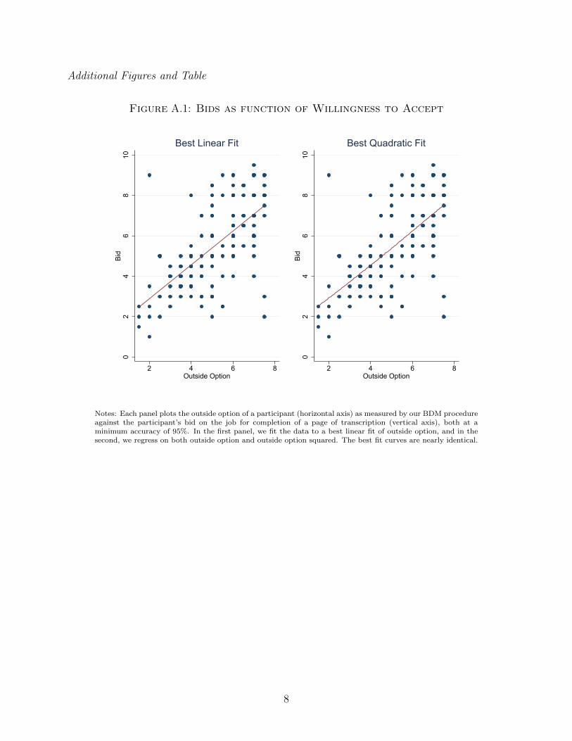
Additional Figures and Table

Figure A.1: Bids as function of Willingness to Accept

02

46

810

Bid

2 4 6 8Outside Option

Best Linear Fit

02

46

810

Bid

2 4 6 8Outside Option

Best Quadratic Fit

Notes: Each panel plots the outside option of a participant (horizontal axis) as measured by our BDM procedureagainst the participant’s bid on the job for completion of a page of transcription (vertical axis), both at aminimum accuracy of 95%. In the first panel, we fit the data to a best linear fit of outside option, and in thesecond, we regress on both outside option and outside option squared. The best fit curves are nearly identical.

8

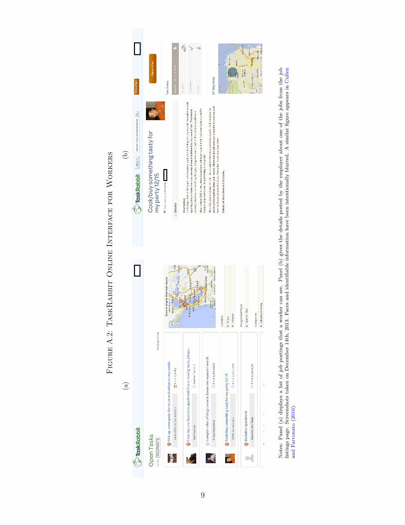
Figure

A.2

:Task

Rabbit

OnlineIn

terfa

ceforW

orkers

(a)

(b)

Note

s:P

an

el(a

)d

isp

lays

ali

stof

job

post

ings

that

aw

ork

erca

nse

e.P

an

el(b

)giv

esth

ed

etails

post

edby

the

emp

loyer

ab

ou

ton

eof

the

job

sfr

om

the

job

list

ings

page.

Scr

een

shots

taken

on

Dec

emb

er14th

,2013.

Face

san

did

enti

fiab

lein

form

ati

on

have

bee

nin

tenti

on

ally

blu

rred

.A

sim

ilar

figu

reap

pea

rsin

Cu

llen

an

dF

arr

on

ato

(2016).

9

TABLE A.6: Worker-Bid Level Pay Compression, TaskRabbit

(1) (2) (3) (4)

Dep. Var. Final Pay (% over bid)

Distance from Top Bid (%) 0.384*** 0.385*** 0.388*** 0.283**[0.137] [0.137] [0.138] [0.135]

X Separated -0.364*** -0.366*** -0.367*** -0.275**[0.139] [0.140] [0.140] [0.137]

X Virtual -0.306** -0.307** -0.304** -0.189[0.141] [0.141] [0.142] [0.141]

Separated -0.00228 0.00307 0.0235 -0.0168[0.0512] [0.0520] [0.0420] [0.0565]

Virtual -0.0359 -0.0289 0.00416 -0.112[0.0493] [0.0498] [0.0484] [0.0765]

WorkerTraits

Worker months experience 0.849 0.584 -0.204[1.439] [1.304] [1.252]

Prior # closed offers -0.000425 -0.00305 0.00822[0.00751] [0.00839] [0.00884]

Female (yes = 1) -0.0288 -0.00725 -0.0125[0.0200] [0.0198] [0.0216]

Job&Empl.Traits

No. workers (log) -0.0501** -0.0575**[0.0201] [0.0240]

Length of job post (log) 0.0424 0.00189[0.0390] [0.0197]

Freq. of task category (log) -0.0389 0.00654[0.0346] [0.0194]

Required equipment 0.383 0.0210[0.493] [0.0997]

Business (incorp.= 1) -0.0495[0.0659]

Business (unclassified) 0.0654[0.0845]

Constant 0.0616 0.0698 0.231 0.173[0.0461] [0.0526] [0.336] [0.233]

Category FE X XEmployer FE X

Mean Dep. Var. 0.115 0.115 0.115 0.115Observations 3235 3235 3232 3232Clusters 464 464 464 464R2 0.172 0.173 0.198 0.583

Notes: Each model is estimated by OLS. An observation is an accepted worker-bid for a multi-worker job onTaskRabbit. Standard errors are clustered at the level of the employer. The dependent variable is the size of theraise, as percent above the worker’s initial bid. The primary explanatory variable is an interaction between thedistance the initial bid is from the maximum bid selected and a categorical variable for co-located, separatedor virtual workers.

10

B. Theoretical Appendix

B.1. Firm acceptance and rejection of offers

We introduced the game as one in which the firm selects a single w and is bound to thatfor all time. More realistically, the firm may be able to accept offers on a case-by-case basis.In this section, we show that generalizing the game and restricting our attention to a classof time consistent equilibria does not change the analysis.

Ammendments to the timing of the stage game are straightforward. Instead of selectingw at t = 0, the firm selects “accept” or “reject” for each offer as it receives it. By accepting,the firm is locked in to paying the agreed upon wage until the worker departs or makesanother offer, and if the firm rejects, then the worker is inelligible to work at the firm.

As we are interested in the effect of transparency on wage negotiation, learning aboutthe wages of others must convey information about the wage a worker can request. Intu-itively, we want to use an equilibrium refinement like Markov perfection, as this includessubgame perfection (so that the firm cannot make non-credible threats of refusing to acceptcertain wage offers) and time consistency (seeing the wage of a higher paid co-worker meansthat a worker knows she can receive that wage if she offers it to the firm). Unfortunately,Markov perfect equilibria are not well-defined in our setting.45 Formally, we study equilibriasatisfying A0, A1-3, A4’, and A5. We define A0 and A4’ below.

A0 The firm selects some function w(v), and accepts all offers wi,t ≤ w for any worker i andany time t, and rejects all others.

A4’ Let wsupt be the highest wage paid by the firm at time t if the worker observes wages

at time t, and 0 otherwise. Off path, each worker i believes with probability 1 thatthe firm will accept any offer she makes that is no more than max{w∗i , w

supt } and will

reject all greater offers.

A0 restricts attention to firm strategies that set a maximum wage w that is constant acrossworkers and over time within worker. This assumption that the firm’s strategy is time-consistent within worker is a Markovian restriction; a firm can condition its acceptancestrategy on v, previous offers made by the worker, and the history of the game. Notehowever, that given the constant inflow and outflow of workers, the only payoff relevantfactor determining the state of the game from the firm’s point of view is v. Furthermore,this Markovian assumption is necessary to understand the effects of pay transparency andworker bargaining. Because each worker is infinitesimally small, without any restriction, thefirm could essentially negate pay transparency by refusing to renegotiate with workers. Forexample, the firm could play a strategy that defines some wi,t(v), which is the maximumwage it will accept from each i at time t. The firm could set wi,t = v and wi,t′ = w∗i for all

t′> t, which corresponds to the “full secrecy” world of λ = 0 we present later. Without

this restriction, it is also possible to construct “sun spot” equilibria in which wt(v) is a stepfunction in t, that is at some time t

′the firm’s maximum willingness to pay jumps upward.

The restriction that the maximum accepted offer is equal across workers is motivatedby the assumption that the firm cannot wage discriminate against workers as it does not

45Watson (2016) discusses some issues of equilibrium refinement in games with infinite action spaces.

11

observe outside options.46 As we have limited our study to equilibria in which the firm’swillingness to pay is constant over time within worker, if the firm had a different willingnessto pay across workers, it would imply that the firm has a different willingness to pay fortwo workers i and j at the moment each of these workers enters the market. Due to lackof information about outside options, the firm cannot discriminate in this fashion over apositive measure set of workers in equilibrium. We formally include the assumption that themaximum accepted offer is equal across workers here to rule out equilibria which vary onlyupon a measure zero set of workers.

A4’ is a special case of A4 and states that off path, conditional on learning the wages ofco-workers, workers believe they can receive no more than wsup

t and will not be rejected if theyoffer wsup

t . In other words, workers believe that even off path the firm plays a time consistentstrategy as in A0. Although outside our model, such beliefs are potentially reasonable inthe presence of equal pay laws.

All of the results in the paper go through under this expanded game if we restrict attentionto equilibria satisfying the above conditions. Indeed, all of the results until those in SectionIII.D. go through if relax off path beliefs in A4’ to workers believing that with probability1 that any offer weakly less than wsup

t will be accepted. Nevertheless, this relaxed versionof A4’ can create an additional equilibrium outcome in the game with endogeneous firmselection of transparency in which all firm types pool on Λ = 0. Further details are availablefrom the authors upon request.

B.2. Double Auction Mapping

This section shows the steps transforming Equation 1 into Equation 2. For λ ∈ [0,∞)

argmaxw∗i

(w∗i

ρ+δ+λ+ λ

ρ+δ+λ

E(w|w≥w∗i )δ+ρ

)(1− F (w∗i )

)+ θi

δ+ρF (w∗i )

= argmaxw∗i

(w∗i

ρ+δρ+δ+λ

+ λρ+δ+λ

E (w|w ≥ w∗i )) (

1− F (w∗i ))

+ θiF (w∗i )

= argmaxw∗i

(w∗i

ρ+δρ+δ+λ

+ λρ+δ+λ

E (w|w ≥ w∗i )− θi) (

1− F (w∗i ))

= argmaxw∗i

((1− Λ)w∗i + ΛE (w|w ≥ w∗i )− θi)(1− F (w∗i )

)= argmax

w∗i

´ 1

w∗i((1− Λ)w∗i + Λx− θi) f(x)dx

(11)

where Λ = λρ+δ+λ

. When λ = ∞, the scheme is equivalent to a posted price in which

Λ = 1 (workers receive w if they remain at the firm). Therefore, for any ρ, δ > 0 there is abijection between λ and Λ with higher Λ corresponding to more transparency.

46Massachusetts recently passed a law prohibiting firms from asking potential employees their cur-rent salaries during job interviews (http://www.nytimes.com/2016/08/03/business/dealbook/wage-gap-massachusetts-law-salary-history.html accessed 11/7/2016) and employers often have little information onworkers’ outside options in online labor markets such as TaskRabbit. Even if firms are able to observe demo-graphic factors associated with high or low outside options (perhaps such as gender), and would optimallyset a different maximum wage for these groups, any such strategy would be in violation of the Equal Pay Actof 1963, opening up the firm to litigation. Therefore, the analysis would be unchanged if instead the firmcould observe the demographics of workers but could not select separate wage policies for different groups.

12

C. Omitted proofs

Proof of Proposition 1:

It is easy to see that for all times t ≥ 0 there exists at least one worker earning w.Therefore, conditional on receiving wage information, every worker will offer the highest wagevisible which equals w. It remains prove that in equilibrium a worker will never renegotiatewithout the arrival of wage information. Without loss of generality, let a worker enter themarket at t = 0 and (in an abuse of notation) let ws denote the wage the worker offers at times in the absence of arrival of wage information. If the worker does not renegotiate betweentimes t

′and t

′′then let ws = wt′ for all s ∈ [t

′, t′′]. Therefore, w is a non-decreasing sequence

bounded above by 1. Consider a strategy which dictates in the case of no information arrivalthat wt′ > w0 for some t

′> 0, such that the worker’s expected discounted future surplus at

any time s is non-decreasing (this latter condition is clearly necessary for any equilibriumstrategy). Consider a “compression” strategy which differs only that sequence w is replacedby wφ for φ > 1 such that wφs = wφ·s.

If w is increasing at t = α · s then this also increases the worker’s expected discountedfuture surplus by the equilibrium hypothesis. But then increasing wα at t = s does so aswell. Then the compression strategy increases the worker’s payoff. Proceeding inductively, itis easy to see that taking α→∞ (i.e. full compression) is the optimal compression strategyfor any w. But the expected payoff from such a compression converges to the payoff fromsetting ws = lim

t→∞wt for all s > 0. Therefore, the optimal strategy sets ws = w∗ for all s ≥ 0

and some w∗ ∈ [0, 1].

�

Proof of Proposition 2:

Let w = β(v) and let w∗i = γ(θ) and assume that a linear equilibrium exists. Workers arehired at initial wages in some range [a, h] where 0 ≤ a ≤ h ≤ 1. By the linearity hypothesis,it must be the case that

w =

{v 0 ≤ v < a

a+ h−a1−a (v − a) a ≤ v ≤ 1

w∗i =

{a+ h−a

hθi 0 ≤ θi ≤ h

θi h < θi ≤ 1

(12)

Furthermore, by definition F (x) = P (β(v) ≤ x) = F (β−1(x)), and similarly G(x) =G(γ−1(x)). Inverting the functions in Equation 12 and plugging in to the distributions inEquation 7 yields

F (x) = 1−(

1− a+ (x−a)(1−a)h−a

)rG(x) =

((x−a)hh−a

)s a ≤ x ≤ h (13)

13

Equations 5 and 6 give another set of equations for γ−1(·) and β−1(·). Plugging these into the distributions in Equation 7 yields

F (x) = 1−(

1− x− Λ G(x)g(x)

)rG(x) =

(x− (1− Λ)1−F (x)

f(x)

)s a ≤ x ≤ h (14)

Solving Equations 13 and 14 simultaneously results in a unique solution in which

a = (1−Λ)s(s+Λ)r+(1−Λ)s

h = (1−Λ)s+rs(s+Λ)r+(1−Λ)s

(15)

As w and w∗i are pinned down by a and h due to linearity, there is a unique linearequilibrium.

�

Proof of Proposition 3:

The proof of the first two points follows from noting that 1−F (x)

f(x)= h−x

rand g(x)

G(x)= s

x−afor all x ∈ [a, h]. Both of these terms are strictly decreasing indicating the desired resuilts.

The third and fourth points remain to be shown. We first show w is strictly decreasingin Λ for all v ∈ [a, 1]. Using Equations 12 and 15, we see that

w = a+ ss+Λ

(v − a) for all v ∈ [a, 1] (16)

Differentiating with respect to Λ yields

∂w

∂Λ=

∂a

∂Λ

(1− s

s+ Λ

)− s

(s+ Λ)2 (v − a) (17)

Noting that ss+Λ∈ (0, 1] and that from Equation 15

∂a

∂Λ

sign= −r(s+ 1) < 0 (18)

implies that ∂w∂Λ

< 0 for all v ∈ [a, 1]. From Equation 13 we see that G(x)g(x)

= x−as

for all

x ∈ [a, h]. Therefore, from Equation 6 we see that w → v for all v ∈ [0, 1] as Λ→ 0.By virtue of the fact that w is decreasing in Λ, it must also be the case that h is decreasing

in Λ. (It is possible to directly verify this by computing ∂h∂Λ

.) From Equation 13 we calculate1−F (x)

f(x)= h−x

rfor all x ∈ [a, h]. Since h is decreasing in Λ, 1−F (x)

f(x)is also decreasing in Λ over

this range. Therefore, from Equation 5 we see that w∗i is strictly decreasing for θi ∈ [0, h],and w∗i → θi for all θi ∈ [0, 1] as Λ→ 1.

�

14

Proof of Theorem 1:

1. For all θk < h we have from Equation 12 that w∗k = a + h−ahθk. Therefore, for any

relevant workers i and j, we have that w∗i − w∗k = h−ah

(θi − θj) . From Equation 15 wesee that the derivative of this function is increasing in Λ, completing the claim.

2. Recall from Equation 11 that the expected lifetime earnings of a worker with outsideoption θi is T (Λ, v, θi) = (1− Λ)w∗i + Λw − θi. A sufficient condition for T (·, v, θi) −T (·, v, θi) being strictly decreasing in Λ is that ∂2T (Λ,v,θ)

∂θ∂Λ< 0 for all Λ, θ ∈ [0, 1) and all

v ∈ [0, 1]. From Equations 11 and 12 we see that

∂2T (Λ, v, θ)

∂θ∂Λ=∂(1− Λ)h−a

h

∂Λ(19)

From Equation 15 we see that

∂(1− Λ)h−ah

∂Λ=∂(1− Λ) r

r+(1−Λ)

∂Λ=

−rr + 1− Λ

(20)

Since Λ, r > 0 we see that ∂2T (Λ,v,θ)∂θ∂Λ

< 0 as desired. To show that T (·, v, θi) −T (·, v, θi) → 0 in Λ, we note that T (·, v, θi) = (1− Λ)w∗i + Λw. Since w∗i is boundedbelow by θi then T (·, v, θi) converges to w(Λ) for any θi.

�

Proof of Theorem 2:

1. To see the equilibrium employment level of the firm, we calculate the probability thata worker is hired by the firm ex-ante. Let E(r, s,Λ) be the expected equilibriumemployment level in a market with distribution parameters r and s and transparencyΛ. Then

E(r, s,Λ) ≡´ h

0Pr (w ≥ w∗i (θ)) g(θ)dθ

=´ h

0Pr(v ≥ a+ 1−a

hθ)g(θ)dθ

= s · (1− a)r´ h

0

(1 + 1

hθ)rθs−1dθ

= (1− a)r hs Γ(r+1)Γ(s+1)Γ(r+s+1)

(21)

where the first equality comes from substituting in Equation 12, the second equalitycomes from substituting in the distribution of outside options from Equation 7 and thethird from Γ(x) ≡

´∞0yx−1e−ydy. As we see, transparency affects employment through

changing a and h. We know from Equation 21 that

15

argmaxΛ

E(r, s,Λ) = argmaxΛ

(1− a)r hs (22)

Substituting in from Equation 15 and taking the first order condition with respect toΛ yields

Λ∗ =r + 1

r + s+ 2(23)

It remains to show that the maximization problem in Equation 22 is concave in Λ over[0,1]. Taking the first order condition of Equation 22 we see that

∂(1− a)rhs

∂Λ= −r

2s2(1− a)r−1hr−1(r(Λ− 1) + (2 + s)Λ− 1)

(s(1 + r − Λ) + rΛ)3(24)

From this, since r, s > 0 and a < 1 we see that the first order condition in Equation23 holds. Substituting in from Equation 7 gives us the particular form of Λ∗ in thetheorem. We further can calculate

∂2(1− a)rhs

∂Λ2

sign= −rshs(1− a)r

(s3(r2 + r

(2− Λ2

)+(1− Λ2

))−rΛ

(r2(2− Λ) + 2r

(Λ2 − 3Λ + 2

)+(4Λ2 − 5Λ + 2

))−s2

(r3 + r2

(−2Λ2 + 2Λ + 2

)+ r

(−2Λ2 + 4Λ + 1

)+ 2Λ

(1− Λ2

))−s(r3(−Λ2 + 2Λ + 1

)+ r2

(3− 2Λ2

))−s(r(6Λ2 − 6Λ + 3) +

(−4Λ3 + 7Λ2 − 4Λ + 1

))A sufficient condition for ∂2(1−a)rhs

∂Λ2 < 0 for all Λ ∈ (0, 1) is that each of the polyno-mial terms involving Λ be strictly positive for Λ ∈ (0, 1). It is easy to check each ofthese polynomials separately to see that this sufficient condition is indeed satisfied.Therefore, extreme point Λ∗ is the global maximizer of expected employment.

2. In equilibrium, there is an outside option cutoff for employment θ∗ such that all workerswith outside options weakly less than θ∗ negotiate wages that are acceptable to thefirm. Then employment is equal to G(θ∗). Noting that a worker i with outside option θ∗

sets w∗i = w it must be the case that G(θ∗) = G(w). We show that G(w) is submodularin v and Λ, and rely on monotone comparative statics techniques of Topkis (1998) tocomplete the result. From Equations 12 and 13 it is the case that for all v ≥ a

G(w) =

(h

1− a(v − a)

)s(25)

We can use a monotonic transformation of G(w) to complete the claim, that is, weshow submodularity of h

1−a(v − a) in v and Λ.

16

∂ h1−a(v − a)

∂v=

h

1− a=

(1− Λ)s+ rs

(s+ Λ)r(26)

Which is clearly decreasing in Λ. Therefore, G(w) is submodular in v and Λ.

�

Proof of Theorem 3:

We show that the expected equilibrium profit of the firm is strictly increasing in Λ. Thatthe expected equilibrium profit of an arbitrary worker is strictly decreasing in Λ follows asimilar calculation. We invoke the law of iterated expectations by first finding the firm’sprofit for a particular draw v > a which we denote by π(v,Λ).

π(v,Λ) =

w

a

(v − (1− Λ) y − Λw) g(y)dy

=

w

a

(v − (1− Λ) y − Λw) s

(h

h− a

)s(y − a)s−1dy (27)

=(w − a)s

s+ 1

(h

h− a

)s(a (Λ− 1)− w(Λ + s) + sv + v)

where the second equality comes by using Equation 13. The ex-ante expected profit of thefirm can be expressed as π(Λ) =

´ 1

aπ(v,Λ)f(v)dv. A tedious, but straightforward calculation

shows that ∂π(Λ)∂Λ

> 0 for all r, s > 0 as desired.

�

Increasing transparency does not increase profits for all firm types:

Example 1. Let v = 1 and let E(θ) = E(v) = 12. This implies that r = s = 1. We can

calculate the profit π(v,Λ) of the firm using Equation 27. We see that π(1, 1) = 12

whileπ(1, 1

2) = 9

16.

�

Proof of Theorem 4:

We begin this proof with a lemma.

Lemma 1. Let M denote the worker belief that the firm will select Λ = 1 in equilibrium.Then if M < 1 and Λ = c and Λ = d with c < d are each chosen with positive probability(density) then with positive probability a positive mass of workers will renegotiate wagesbefore learning w, unless c = 0 and d = 1.

17

Proof of Lemma: We assume c and d are chosen with positive probability, but the proof issimilar if these are instead selected with positive densities.

0 ≤ c < d < 1 : We prove this case by contraposition. Suppose the set of workers who rene-gotiate wages before learning w has zero measure. Then playing Λ = d gives a strictlylower profit than Λ = c, as it does not change initial bids and only increases the rate atwhich the firm must pay workers w. Therefore, any firm setting Λ = d has a profitabledeviation instead playing Λ = c, meaning that d cannot be played in equilibrium.

0 < c < d = 1 : By the previous case we know that there is no e ∈ [0, 1) \ {c} that is chosenwith positive probability. Therefore, if Λ = 1 almost every worker will receive w inthe instant they arrive at the firm (and therefore never renegotiate) and if Λ = cevery worker will believe with probability 1 that Λ = c. Therefore, when Λ = c ischosen worker beliefs do not drift over time so by Proposition 1 each worker will againnegotiate in the instant they arrive and the instant in which they learn w. But thenany firm setting Λ = c has a profitable deviation of instead playing Λ = 0, meaningthat c cannot be played in equilibrium.

�

To complete the proof of the theorem, suppose for contradiction that there is an equilib-rium in which Λ = 0 and Λ = 1 are played with probabilities p0 and p1 where p0 > 0. Thenlet vL be the infemum of the firm types that selects Λ = 0 with positive probability. When afirm plays Λ = 0 almost all workers (except the zero measure set who learns w in the instantthey are hired) correctly deduce the firm choice, and that v ≥ vL. Since v = w when Λ = 0,each worker will set w∗i ≥ vL. Take a sequence {v`}`∈N → vL from above. Then for any ε > 0there exists some `∗ such that for all ` > `∗, v` − vL < ε. Then any firm type v` with ` > `∗

will receive strictly less than ε profit per worker it employs when it follows the equilibriumprescription and sets Λ = 0. Letting ε → 0, any of these firm types with v` − vL < ε canmake higher total profits by selecting Λ = 1 and setting w = v

2. Therefore, there can be no

such equilibrium in which p0 > 0. By inspection, we have exhausted all cases except that inwhich p1 = 1. To see that an equilibrium exists in which no worker renegotiates wages andall firms select Λ = 1, consider the worker belief that Λ = 0 and v = 1 upon not seeing thewages of co-workers at the instant they are hired. The optimal response to these beliefs isto set w∗i = 1 for all i, meaning that the firm will make zero profits if it deviates.

�

Proof of Proposition 4:

Suppressing time and worker indices, suppose a worker has negotiated a flow wage of w.Then in addition to her other choices, she must choose e to solve max

e∈[0,1]w · e− θ · e. For any

w ≥ θ the maximizer is e = 1.47 Therefore, when w ≥ θ the equilibrium flow utility to the

47Of course, if w = θ any e ∈ [0, 1] is a maximizer. For our purposes, we select e = 1 in this case, although,as we see, in equilibrium this will only affect a zero measure set of workers.

18

worker is w − θ, as in the initial model. But by A1 a worker would never agree to a wagew < θ. So in equilibrium, e = 1 and payoffs are the same as the original model. It is easy tosee that given this, all other equilibrium choices will be unchanged.

�

Proof of Proposition 5:

We prove the second part of the proposition as the first is easy to see.

⇒ Clearly it cannot be the case that m(e, d) = 0 for some d > 0, or else the firm wouldnever fully equalize wages. Suppose for contradiction that w ·e−θ ·e−m(e, d) = ε > 0for some e, d. Let e∗(d, w∗i , w) be the optimal effort selected by worker i upon learningw and receiving wage w∗i . The firm must solve

maxw−w∗i≤d≤0

e∗(d, w∗i , w)(v − w + d) (28)

SF1 and SF2 imply that for any Λ, v, w and w∗i , d = 0 is optimal, inducing e = 1.This implies that

v − w ≥ e∗(d, w∗i , w)(v − w + d) ∀Λ, d, w, v, w∗i (29)

which holds if and only if

v − w ≥ d · e∗(d, w∗i , w)

1− e∗(d, w∗i , w)∀Λ, d, w, v, w∗i (30)

Consider a firm of type v = 1 and a worker of type θi = 0. By sending r →∞, h−a→ 1.By sending Λ→ 0, the LHS of Equation 30 converges to 0, while by assumption thereexists some d for which the RHS is bounded away from 0. Contradiction.

⇐ This direction is easy to see. If w · e − θ · e − m(e, d) ≤ 0 for any e ∈ [0, 1] and anyd ∈ (0, 1] then as soon as any worker learns w the firm can either choose to increaseher wage to w and receive flow profits v − w ≥ 0 or receive flow profits of 0 otherwisefrom the worker who will put in zero effort.

�

Proof of Proposition 6:

Taking the first order condition of Λm − Λf with respect to λ yields

αmαf

=(ρ+ δ + αmqλ)2

(ρ+ δ + αfqλ)2 (31)

19

The LHS of Equation 31 is constant in λ while the RHS is increasing in λ as αm > αf .Therefore, there is a unique solution λc to this first order equation and thus a unique interiorextreme point. As Λm − Λf > 0 for all λ ∈ (0,∞) and it is continuously differentiable overthis domain, the fact that Λm − Λf = 0 for λ ∈ (0,∞) it must be that λc is a maximizer,and that Λm − Λf is single-peaked.

�

D. Multiple firms

In this section, we embed our analysis of pay transparency into a search model by in-cluding multiple firms, and show that many of the insights of the main model carry over tothis setting. For tractibility, we study only the cases of full secrecy and full transparency.Let N = {1, 2, ..., N} be the set of firms, each with a value for labor vn drawn iid from dis-tribution F. As before, workers have outside options drawn iid from distribution G. Workersnegotiate with firms in a predetermined order without the possibility of returning to anearlier firm. Without loss of generality, we assume that workers first meet with firm 1, thenfirm 2, and so on.

If a firm rejects a worker’s offer the two are ineligible to match at any point in thefuture, and the worker (instantly) moves to the next firm in the sequence. Although wedo not do so for simplicity of exposition, it is possible to embed a search friction in thisformulation without affecting the qualitative findings.48 A worker whose offer is rejectedby firm N becomes unemployed for her duration in the market and consumes her outsideoption. Workers continue to expire at rate ρ at which time they leave the market. A workerwhose offer is accepted by firm n < N is replaced with a worker of identical outside optionwho moves on to firm n+ 1 as if her offer had been rejected at firm n.49

Each firm n selects a maximum wage it is willing to pay for a worker wn(vn) ∈ [0, 1],where the choice of wn is not immediately observed by workers. As before, each workerbargains for wages by making TIOLI offers to firms at any point during her employment,potentially renegotiating infinitely often. Workers who at anytime offer a wage greater thanwn to firm nare permanently unmatched with the firm. Let W n

t denote the set of wagesfirm n is paying to its employed workers, where W n

0 = {wn}. We model transparency as arandom arrival process; at time t, workers matched to firm n matched workers observe W n

t

48Each time a worker’s offer is rejected, we could instead make the worker unable to meet with subsequentfirms with probability ζ ∈ (0, 1). Similarly to the relation between λ and Λ in the main body of the paper,the equilibrium consequences of this probabilistic search friction are identical to a friction which governs the(average) length of time it takes for a worker to find the next firm; in this context ζ close to 0 correspondsto near-instant discovery of the next firm, while ζ close to 1 corresponds to near-infinite time required todiscover the next firm. Including such a search friction does not meaningfully change the remainder of theanalysis.

49This assumption is made for tractability as this “cloning” greatly simplifies equilibrium characterizationin our context, and is frequently adopted in the search literature (see, for example, Burdett and Coles (1999),Bloch and Ryder (2000), and Chade (2006)). This assumption may be even more defensible in a setting likeTaskRabbit, in which jobs are short-term, and therefore, we can interpret a “cloned” worker as merely aworker who has completed a given task and is not eligible to re-complete it.

20

according to an independent Poisson arrival process with rate λ ∈ {0,∞}, where we takeλ =∞ to mean that the process arrives whenever a worker first matches with a firm.

The timing of the stage game is as follows at each time t ≥ 0:

1. Entry: New workers enter the market. Initialize m = 1, and `i = 1 for each newworker.

2. Search and Bargaining:

(a) Unmatched workers match with firm m if `i = m.

(b) Each matched worker i learns Wmt independently with arrival rate λ.

(c) Newly entering workers must bargain with the firm and any existing, matchedworker can initiate bargaining. Any worker i who engages in bargaining makesa TIOLI offer wmi,t ∈ [0, 1] to firm m. If wmi,t ≤ wm then firm m pays i a flowwage wmi,t until i departs or attempts to renegotiate. If wmi,t > wm then worker ibecomes unmatched.

(d) For any i such that wmi,t > wm increase `i by 1.

(e) If m < N , for all i such that wmi,t ≤ wm, create a new worker j with θj = θi and`j = `i + 1, increase m by 1 and repeat Step 2.

3. Exit: Existing workers depart at rate ρ.

D.1. Equilibrium

We work backward to solve for the unique equilibrium. Workers meeting firm N facethe same decision as workers in the base model: they face a firm with value vN drawnfrom distribution F and are among an incoming cohort with ouside options determined bydistribution G. We know from Equations 5 and 6 that under full secrecy each worker i willoffer firm N an initial amount wNi solving

wNi − θi =1− F (wNi )

f(wNi )

and firm N will set wN = vN . Workers will not attempt to renegotiate. Under fulltransparency, N will set wN to solve

vN − wN =G(wN)

g(wN)

and worker i will be employed at flow wage equal to wN if and only iff wN ≥ θi. Denote byθn,λi the expected equilibrium lifetime utility (under transparency level λ) of a worker withoutside option θi immediately upon matching with firm n (before making an offer or learningwages through the transparency process), and denote by Gn,λ the distribution of θn,λi . Then,when facing firm N − 1, workers face will face the same decision but with θi replaced with

21

θN,λi , and firm N − 1 will face the same decision as firm N but with distribution G replacedwith GN,λ. Inducting up toward the first firm, we can characterize the equilibrium actionsof agents as the following:

λ = 0 :

Workers:

wni − θn+1,0i =

1− F (wni )

f(wni )for n < N (32)

Firms:

vn = wn for n ≤ N. (33)

λ =∞ :

Workers:wni = wn1{wn≥θn+1,∞

i } for n < N (34)

Firms:

vn − wn =Gn+1,0(wn)

gn+1,0(wn)for n < N. (35)

As θi is constant over time, θ·,λi is a non-increasing sequence, and strictly decreasing for

workers with θi < 1. Therefore, G·,λg·,λ (x) is non-increasing in n. In words, workers’ outside

options, which include the option value of bargaining with future firms, decreases as theymove along the sequence of firms. Realizing this, under full transparency, earlier firms accepthigher wages to incentivize workers to accept their offers rather than wait to meet futurefirms. We now provide results that are similar to the theorems in the main text.

Proposition 7. The expected average utility of workers is higher in equilibrium with λ = 0than λ =∞. The expected utility of firms is higher in equilibrium with λ =∞ than λ = 0.

Proof:

We prove this result for workers, and the converse for firms is similar. By Myerson (1981)the expected utility of any worker who reaches firm N is higher under λ = 0 than λ = ∞.Therefore, θN,0i > θN,∞i for all θi. When meeting firm N−1, worker θi is in expectation betteroff setting offering wN−1

i solving

wN−1i − θN,∞i =

1− F (wN−1i )

f(wN−1i )

(36)

22

than receiving the equilibrium offer under full transparency by the same Myerson (1981)argument. That worker i is able to offer wN−1

i but instead chooses wN−1i that solves Equation

32 indicates that worker i is better off in expectation by revealed preference under full secrecy.By induction, we see that worker i is better off at every firm she meets under full secrecy.

�

Below are three analogues of the remaining theorems in the body of the paper. Theproofs are omitted as the logic follows the proofs of the main theorems.

Proposition 8. When λ = ∞ there is no wage dispersion between workers at the samefirm in equilibrium.

Proposition 9. The ex-post employment maximizing level of transparency is weakly de-creasing in v.

Proposition 10. When each firm can select λ ∈ {0,∞} as a function of v there is anessentially unique equilibrium outcome. In equilibrium, each firm selects λ = ∞ for allv > 0.

E. Negotiation extensions

In this section, we discuss alternative bargaining protocols that generate qualitativelysimilar findings as the TIOLI bargaining scheme studied in the body of the paper. Thefirst two cases consider situations in which workers are not able to rebargain as effectivelyas in the base model, either by being unable to capture the entire difference between theirinitial offers and w, or sometimes being unable to rebargain. There is an injection betweenthe equilibria of these games and the game studied in the body of the paper, in whichthe additional bargaining friction result in de facto lower levels of transparency. The lastextension shifts the bargaining power from the workers to the firm probabilistically, givingthe firm the ability to propose wages to a fraction of workers.50 We show that the equilibriumoutcome for workers receiving wage offers is independent of the level of transparency, andthe equilibrium outcome for workers proposing wages is identical in this extended game tothat of the original game. Therefore, transparency has the same equilibrium effects in thisgame, just affecting a smaller portion of the workers.

E.1. Workers can only rebargain for part of surplus

There are a number of possibilities as to why workers may not be able to fully close thegap between their initial wage and w. This could arise from a game in which workers and firmengage in alternating offer bargaining with disagreement amounts set to w∗i . It could evenoccur under a worker TIOLI offer scheme under a “non-Markovian” (i.e. does not satisfycondition A0 in Section B.1.) equilibrium in which the firm’s strategy is equilibrium is toreject rebargaining offers that request more than a fixed proportion of the difference between

50This extension is similar to a modeling choice in Halac (2012) which changes the effective bargainingpower of two parties by varying the probability of each agent making a TIOLI offer.

23

a worker’s initial bid and w. Formally, suppose that the firm selects w which is the maximumwage it accepts from any worker in the initial period a worker is hired. At any subsequentperiod, the firm rejects any renegotiation offer strictly greater than w∗i + α(w − w∗i ) whereα < 1.

Proposition 11. The (unique) linear equilibrium of the game in which workers can onlyrebargain for α ∈ [0, 1) fraction of the difference between w and w∗i and transparency levelΛ < 1 is equivalent to that of the original game with transparency level αΛ.

Proof:

For any α the equilibrium of this game is clearly equivalent to that of the original gamewhen λ = ∞ (Λ = 1). When λ < ∞, following the same logic as the main case, workersnegotiate at most twice in equilibrium, once when they are first hired, and once when theylearn w through the transparency process. Letting F (x) = P (w ≤ x), worker i negotiates atthe first moment she is hired to:

argmaxw∗i

(w∗i

ρ+ δ + λ+

λ

ρ+ δ + λ

[w∗i + α

(E (w|w ≥ w∗i )

δ + ρ− w∗i

)])(1− F (w∗i )

)+

θiδ + ρ

F (w∗i )

(37)where the first term represents the weighted (by λ) expected wage the worker receives if

matched with the firm, and the second term represents the lifetime earnings of the worker ifshe exceeds w and instead consumes her outside option for her lifetime.

As before, we modify the objective function without affecting the maximizer, and showthat this is equivalent to solving:

argmaxw∗i

´ 1

w∗i((1− Λ)w∗i + Λ (w∗i + α (x− w∗i ))− θi) f(x)dx

= argmaxw∗i

´ 1

w∗i((1− αΛ)w∗i + αΛx− θi) f(x)dx

(38)

where Λ = λρ+δ+λ

for all λ ∈ [0,∞). In equilibrium, the firm sets w(v) to

argmaxw

´ w0

(v − y) g(y)dy

ρ+ δ + λ+G(w)

λ

ρ+ δ + λ

1

ρ+ δ

v − w

0

yg(y)dy + α

w − w

0

yg(y)dy

(39)

where G(x) = P (w∗i ≤ x). The first term gives the total discounted profits made by thefirm before the workers experience an event (seeing the wage profile or perishing) and thesecond term is the profit made from workers after renegotiating their wages to the maximumallowable level over the rest of their lifetimes in the firm. We can similarly manipulate theobjective as with the worker problem:

argmaxw

w

0

(v − (1− αΛ) y − αΛw) g(y)dy (40)

24

Comparing Equations 38 and 40 to Equations 2 and 4, respectively, completes the proof.

�

The results presented in the body of the paper go through in this setting with minornotational changes. The only significant difference is Theorem 2. When α is sufficientlysmall, the employment maximizing level of transparency may no longer be in the interior. Itis possible to show that there exists ε > 0 such that for all α < ε full transparency maximizesexpected employment if and only if full transparency yields higher expected employmentthan full secrecy. Intuitively, when α is small, workers are unable to effectively rebargain,creating the possibility that full transparency (which requires no rebargaining in equilibrium)maximizes employment.

E.2. Workers are probabilistically able to rebargain

Now suppose that each worker is able to rebargain with probability α after the firstmoment she is matched with the firm. Workers who are able to rebargain can take thesame actions as in the standard game, while the 1 − α fraction of workers who cannotrebargain can take no further strategic actions after specifying w∗i . Workers do not ex-anteknow which type they are, and only realize their type after they make the initial offer to thefirm (simultaneously with acceptance or rejection of offer).

Proposition 12. The (unique) linear equilibrium of the game in which each worker canindependently rebargain with probability α ∈ [0, 1) and transparency level Λ < 1 is equivalentto that of the original game with transparency level αΛ.

Proof:

Similar to the proof of Proposition 11.

�

Just as with the extension in Appendix E.1., the results from the body of the paper gothrough with appropriate modification to Theorem 2.

E.3. Two types of workers, receivers and proposers

For this case, suppose that some known fraction of workers are receivers (we can thinkof these as workers who are bad at bargaining) who are unable to make wage offers to thefirm and receive a wage offer from the firm when they are first hired. If a receiver acceptthe offer, she is locked in to working at the specified wage until she perish. If she rejects,she is permanently unmatched from the firm. The remaining workers operate as before, andmake TIOLI offers (potentially infinitely often) to the firm upon matching. The type of eachworker is independent of θi, and is known to both the worker and the firm.

Proposition 13. The (unique) linear equilibrium of the game in which some fraction ofworkers and receivers and others are proposers is as follows:

25

1. The firm offers all receivers an initial wage of ¯w which is the same as w in the originalgame with Λ = 1,

2. The (unique) linear equilibrium outcome for proposers with transparency level Λ isequivalent to that of the original game with transparency Λ.

Proof:

1. This point follows immediately from the fact that the worker type (proposer or receiver)is independent of θi and that θi is privately known by each worker.

2. As ¯w is the optimal posted price wage, the firm cannot maximize profits if it sets w < ¯w.Therefore, when any proposer receives wage information through the transaprencyprocess, in equilibrium she will learn w ≥ ¯w and will successfully demand a flow wageof w. Therefore, a proposer’s information is not affected by the presence of receivers,and the unique linear equilibrium choices of firm, w, and proposer, w∗i , are unchangedfrom the base model.

�

26

F. Experimental Appendix

Here, we show the experimental interface for workers and managers in our experiment.We show the following treatment: $5 manager budget per page, per worker; common cha-troom (pay transparency), manager is instructed to accept all worker bids below budgetwithout bargaining. Other treatments are similar, with changes on Page 5 of these instruc-tions as described in the main text. Note that we did not actually complete any of thetranscription task for the purposes of this illustration, and so the accuracy on Page 11,Workers is calculated at 0.0% for all pages.

Page 1, All Subjects

27

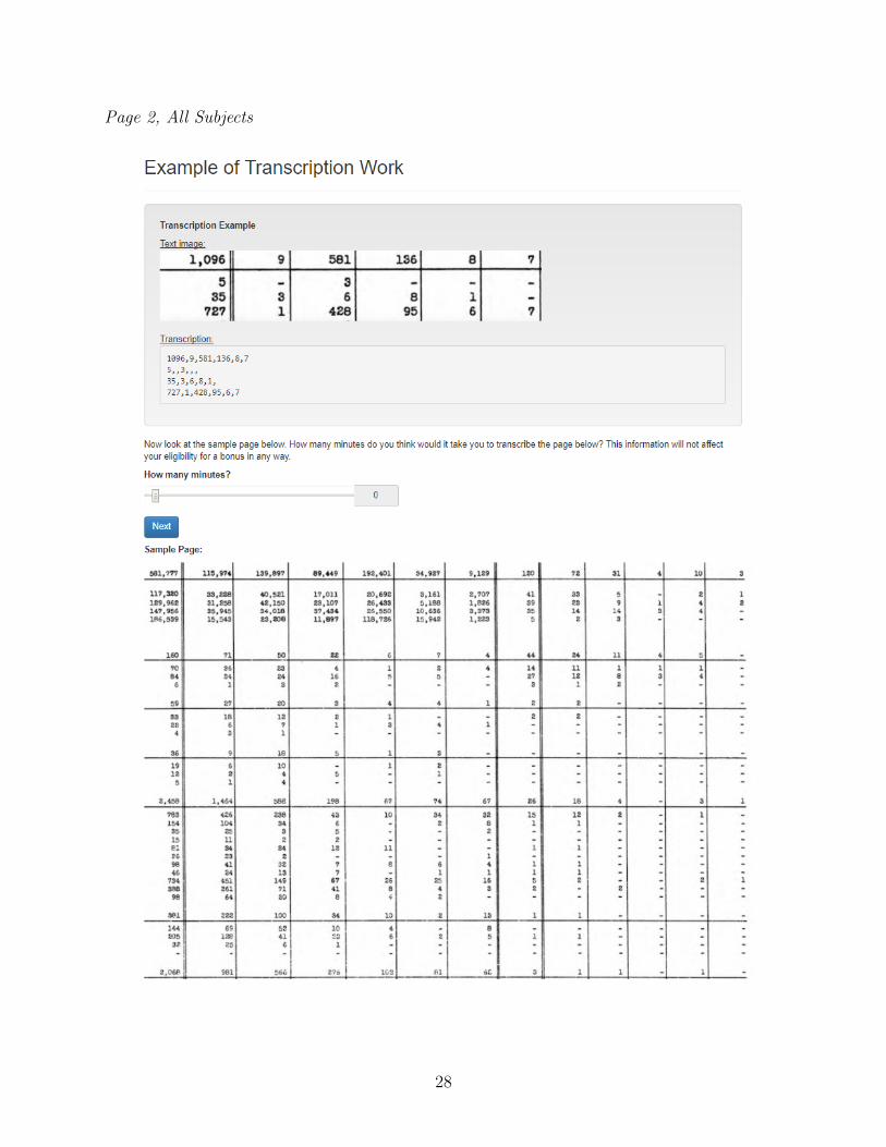
Page 2, All Subjects

28

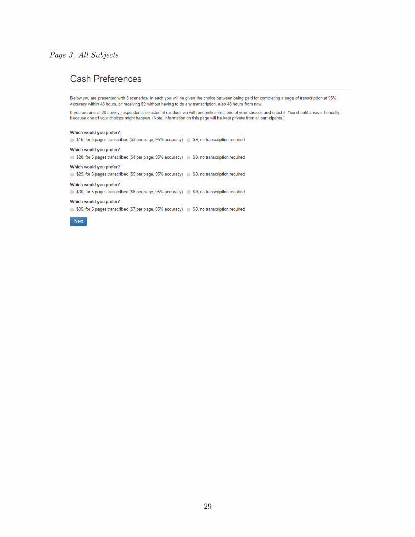
Page 3, All Subjects

29

Page 4, All Subjects

30

Page 5, Manager

31

Page 5, Workers

32

Pages 6-10, Workers

33

Page 11, Workers

34

Page 6, Manager; Page 12, Workers

35

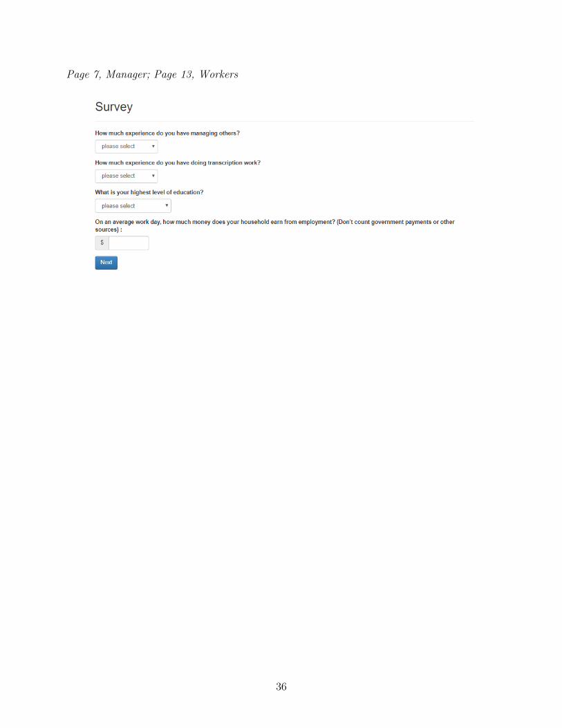
Page 7, Manager; Page 13, Workers

36

Page 8, Manager; Page 14, Workers

37

G. Survey materials

We presented a series of vignettes to approximately 5,000 workers on MechanicalTurk.Each vignette embeds the full job description in a short story about two people that haveplaced private bids for the job, and meet each other for the first time (or do not) uponcommencing the work. The story is followed with four questions that require an answer ona 1 to 10 scale, and a brief explanation; how likely is it that [name] and [name] will discoverwhat the other one is being paid for the same work? that [names] could be a leader or rolemodel and influence the work of [name]? that the employer sees the effort that each of themindividually contributed? and that the same employer would hire [names] in the future fora similar purpose?

We randomly vary the names of the two workers included in the vignette to be soundeither male or female, Alex and Sam or Alexis and Samantha. We also solicit the gender ofthe survey respondent.

G.A. Vignettes

Below we describe a brief posting for a real job that takes place in a real city. Theemployer asks workers on an online labor platform to submit the price they want to completethe job.

Image that two people, Sam and Alex, offer two different prices to do the job. Sam andAlex haven’t met before and they don’t know the other’s price for the job because theysubmitted these offers from their own computers. The employer chooses Sam and Alex onthe platform, and they arrange a time to do the work.

Below is a description of the job. Please read the description and answer the questionsabout what happens when Sam and Alex begin working.

[Insert job description]

Answer on a scale of 0 through 10. A value of 0 means they definitely will not. A value of1 means the odds are 1 in 10. In other words, if it happened 10 times, they would probablyonly learn about each other’s pay on one of those occasions. A value of 10 means that theywould learn about it every time.

1. How likely do you think Sam and Alex will discover what the other one is being paidfor the job?

2. Is this the type of job where either Sam or Alex could be a leader or role model andencourage the other to do a better or worse job?

3. Will the employer be able to see what each of them individually contributed?

38

4. What is the likelihood that either Alex or Sam would be hired by the same employerin the future for something similar?

39