Enhancement of Dynamic Depth Scenes byUpsampling for Precise Super-Resolution (UP-SR)

Kassem Al Ismaeila, Djamila Aouadaa, Bruno Mirbachb, Bjorn Otterstena

a Interdisciplinary Centre for Security, Reliability and Trust (SnT),University of Luxembourg, Luxembourg.

bAdvanced Engineering Department, IEE S.A., Luxembourg

Abstract

Multi-frame super-resolution is the process of recovering a high resolution image or video from a set of captured low resolutionimages. Super-resolution approaches have been largely explored in 2-D imaging. However, their extension to depth videos is notstraightforward due to the textureless nature of depth data, and to their high frequency contents coupled with fast motion artifacts.Recently, few attempts have been introduced where only the super-resolution of static depth scenes has been addressed. In thiswork, we propose to enhance the resolution of dynamic depth videos with non-rigidly moving objects. The proposed approachis based on a new data model that uses densely upsampled, and cumulatively registered versions of the observed low resolutiondepth frames. We show the impact of upsampling in increasing the sub-pixel accuracy and reducing the rounding error of themotion vectors. Furthermore, with the proposed cumulative motion estimation, a high registration accuracy is achieved betweennon-successive upsampled frames with relative large motions. A statistical performance analysis is derived in terms of mean squareerror explaining the effect of the number of observed frames and the effect of the super-resolution factor at a given noise level.We evaluate the accuracy of the proposed algorithm theoretically and experimentally as function of the SR factor, and the level ofcontaminations with noise. Experimental results on both real and synthetic data show the effectiveness of the proposed algorithmon dynamic depth videos as compared to state-of-art methods.

Keywords: Super-resolution, moving objects, non-rigid motion, depth video, upsampling, cumulative motion.

1. Introduction

Interactive computer vision applications using depth datahave literally exploded in recent years thanks to the develop-ment of new depth sensors that are currently accessible to ev-eryone. Most of these applications deal with dynamic scenescontaining one or multiple moving objects. Depth sensors, suchas time-of-flight (ToF) cameras are, however, still limited bytheir high contamination with noise and their low pixel resolu-tions. Moreover, such cameras can be highly sensitive to fastmotions leading to motion artifacts; hence, affecting the relia-bility of depth measurements [1]. Some examples of such cam-eras are the MLI by IEE S.A. [2] of resolution (56 × 61) pixels,and the PMD CamBoard nano [3] of resolution (120×165) pix-els.

Most of the works proposed to enhance the resolution andquality of depth images have been based on fusion with a highresolution (HR) image acquired with a second camera, e.g., a2-D camera [4, 5], a stereo camera [6], or both 2-D and stereocameras [7]. These multi-modality methods suffer from draw-backs such as undesired texture copying, and blurring artifacts.

Email addresses: kassem.alismaeil@uni.lu (Kassem Al Ismaeil),djamila.aouada@uni.lu (Djamila Aouada), bruno.mirbach@iee.lu(Bruno Mirbach), bjorn.ottersten@uni.lu (Bjorn Ottersten)

1This work was supported by the National Research Fund, Luxembourg,under the CORE project C11/BM/1204105/FAVE/Ottersten.

In addition, the performance of these systems depends on pa-rameter tuning, and may encounter difficulties related to datamapping and synchronization.

The multi-frame super-resolution (MFSR) framework offersan alternative solution where an HR image is to be recoveredfrom a set or a sequence of low resolution (LR) images cap-tured with the same camera [8]. The observed LR images aresubject to deviations from the reference image due to relativemotion and to aliasing errors caused by the acquisition system.MFSR can be formulated as an inverse problem where the de-viations on LR frames are explored to estimate the referenceHR image. Super-resolution (SR) techniques have been largelyexplored in 2-D imaging. However, their extension to depthdata is not straightforward as presented in [9, 10, 11] whereonly the SR of a static object has been addressed. The diffi-culty of applying SR to depth videos is further illustrated in thecontext of single image SR (SISR) in [12] where a dedicatedpreprocessing followed by a heavy training were proposed. In-deed, depth data is characterized by its textureless nature withhigh frequency contents. Moreover, fast motions and surfacereflectivity of objects in the scene create invalid pixels and theso-called flying pixels [1]; thus, making most existent 2-D SRalgorithms fail when directly applied on dynamic depth videos.

In this paper, we propose an MFSR algorithm for dynamicdepth scenes. The proposed solution can handle scenes con-taining one or more moving objects even non-rigidly without

Preprint submitted to Computer Vision and Image Understanding April 19, 2015

prior assumptions on their shape, and without training. Ouralgorithm referred to as Upsampling for Precise Super Resolu-tion (UP-SR) builds on our work in [13, 14, 15]. We herein givea unified framework and provide additional details and proofs,and a more extensive experimental part, where we evaluate theaccuracy of the proposed algorithm theoretically and experi-mentally as function of the SR factor, and the level of contami-nations with noise.UP-SR is based on a new data model that uses densely upsam-pled, and cumulatively registered versions of the observed LRframes. It is these two key components, together, that constitutethe working principle of UP-SR as detailed below:1) Upsampling: Most SR algorithms are directly related to aregistration based on a too coarse pixel correspondence as com-pared to the scale of details in the scene. This leads to failurein handling local deformations of moving objects. It is there-fore necessary to call upon a very accurate sub-pixel correspon-dence. In what follows, we argue that this accuracy is signif-icantly increased after upsampling the observed sequence assupported by [16]. Moreover, we prove that the upsamplingprocess reduces the errors caused by rounding the motion vec-tors.2) Cumulative motion estimation: In order to achieve ahigh registration accuracy between non-successive upsampledframes with relative large motions, we propose a new cumula-tive motion estimation process. The proposed method is basedon using the temporal information provided by the intermediateframes between the reference frame and the frame under con-sideration.

The remainder of this paper is organized as follows: Sec-tion 2 reviews state-of-the-art SR techniques in the context oftheir extension to depth data, and to dynamic scenes. Section 3introduces the problem formulation for the classical MFSR. Weprove the improvements in accuracy and robustness due to es-timating motion from densely upsampled depth images in Sec-tion 4. The proposed data model is presented in Section 5 alongwith the proposed cumulative motion estimation, leading to theUP-SR algorithm for dynamic depth scenes with moving ob-jects. Then, a statistical performance analysis is given in Sec-tion 6. Section 7 reports a thorough experimental evaluationof the UP-SR approach and its comparison with state-of-the-art methods. Discussions and conclusion are provided in Sec-tion 8.

2. Related Work

MFSR is the process of recovering an HR image from a set ofcaptured LR frames. It is based on using the deviation betweenthese frames and a reference frame as provided by relative mo-tion, where the ratio between HR and LR defines the SR factor.Depending on the type of motion, two categories of scenes maybe distinguished, and accordingly two categories of SR algo-rithms; SR for static scenes and SR for dynamic scenes. In thestatic case, the motion is global where frames could be seen asslightly different perspectives of the same scene. The scene issaid to be dynamic if there is at least one moving object withnon-rigid deformations; thus, the estimation of a local motion

becomes necessary. In order to understand the challenges re-lated to applying SR to depth data, we review state-of-art ap-proaches for both static and dynamic scenes.

2.1. SR for Static Scenes

The SR estimation is solved numerically using iterativemethods starting from an initial image. This image may be ob-tained by interpolation [17], which is not suitable in the case oftextureless depth data, as interpolating depth data would induceerroneous values and flying pixels that are difficult to attenu-ate. Another approach is known as Shift & Add (S&A) [18, 19]which includes a filling procedure based on the global relativemotion of the considered LR images. Schuon et al. have appliedin [9] the S&A method of [19] to depth images acquired witha ToF camera. In [10], the same authors proposed to replacethe regularization term in [19] by a new term tailored for depthdata, specifically, ToF data, leading to a new depth-dedicatedSR method referred to as LidarBoost. The aim of LidarBoostis to preserve areas with a smooth geometry by using a regu-larization term that is a function of spatial gradients approxi-mated with finite differences. The original LidarBoost uses anL2-norm of weighted depth gradients. In order to better accom-modate the needs of detailed 3-D object scanning, Cui et al.proposed a new version of LidarBoost where the regularizationterm is set to be an anisotropic non-linear function of gradi-ents [11]. In both cases, however, the initial HR is obtainedby means of averaging, which is not appropriate for sensingcluttered scenes. This adaptation of SR to static depth data isquite promising but remains restricted to static scanning wherethe method assumes a perfectly controlled setup with a turningtable-like procedure implying a large motion diversity by con-struction, but not handling non-rigid motions.

2.2. SR for Dynamic Scenes

Dynamic scenes are challenging scenarios for MFSR asthey require the local motion of moving objects to be com-puted accurately. They, hence, may face the problem of self-occlusions especially in the case of non-rigidly moving ob-jects. This difficulty arises in depth videos, but also for 2-Dsequences [21, 22, 23, 24]. Most of the methods in the liter-ature are limited due to strong assumptions on the shape andnumber of moving objects. For this reason, the enhancement ofthe resolution of dynamic depth scenes has been so far mostlybased on fusion with higher resolution 2-D data that has to besimultaneously captured [4, 5]; thus, requiring a perfect align-ment, synchronization, and mapping of the 2-D and depth im-ages, and assuming the correspondence of edges on the twomodalities. These methods may be computationally efficient,but unfortunately they frequently suffer from artifacts causedby the heuristic nature of the enforced statistical model, mainlycopying the intensity texture of 2-D images to depth images.

In this paper, we propose a new MFSR algorithm for dy-namic depth scenes with moving objects. Our algorithm islargely independent of surface texture and does not suffer fromthe texture copying problem since it only deals with LR depthframes as inputs without fusion with any other type of sensors.

2

In what follows, in Section 3, we formulate the problem of dy-namic MFSR.

3. Problem Formulation

The aim of dynamic MFSR algorithms is to estimate a se-quence of HR images {xt0 } of size (

√n ×√

n) from observedLR sequences. The dynamic SR problem can be simplified byreconstructing one HR image at a time, xt0 , for t0 ∈ N using anLR sequence {yt}

t0t0−N+1 of length N, where each LR image yt is

of size (√

m×√

m) pixels, with√

n = r ·√

m, where r is the SRfactor, such that r ≥ 1. Note that for the sake of simplicity, andwithout loss of generality, we assume squared images. Everyimage yt may be viewed as an LR noisy and deformed realiza-tion of xt0 at the acquisition time t, with t ≤ t0. Rearranging allimages in lexicographic order, i.e., column vectors of lengths nfor xt, and m for yt, we consider the following data model:

yt = DHMtt0 xt0 + nt, t ≤ t0, (1)

where D is a matrix of dimension (m × n) that represents thedownsampling operator, and which we assume to be knownand constant over time. The system blur is represented by thetime and space invariant matrix H. The vector nt is an additiveLaplacian noise at time t, as justified in [18, 19]. The matricesMt

t0 are (n × n) matrices corresponding to the geometric motionbetween the considered HR image xt0 and the observed LR im-age yt prior to its downsampling.Based on the data model in (1), and using an L1−norm betweenthe observations and the model, the Maximum Likelihood (ML)estimate of xt0 is obtained as follows:

xt0 = arg minxt0

t0∑t=t0−N+1

‖DHMtt0 xt0 − yt‖1. (2)

Using the same approach as in [19, 27], we consider that H andMt

t0 are block circulant matrices. Therefore: HMtt0 = Mt

t0 H.The minimization in (2) can then be decomposed into two steps;initialization by estimating the blurred HR image zt0 = Hxt0 ,followed by a deblurring step to recover xt0 . In what fol-lows, we assume that yt is simply the noisy and decimatedversion of zt without any geometric warp. We may thus writeMt

t = In,∀t, In being the identity matrix of size (n × n), hence,Mt

t0 zt0 = zt = Hxt. This operation can be assimilated to regis-tering zt0 to zt. We draw attention to the fact that in the case ofstatic MFSR, instead of a sequence, a set of observed LR im-ages is considered, i.e., there is no order between frames. Suchan order becomes crucial in dynamic SR because the estima-tion of motion, based on the optical flow paradigm, happensbetween consecutive frames only. An accurate dynamic SR es-timation is consequently highly dependent on the accuracy ofestimating the registration matrices between consecutive framesMt−1

t , as well as the motion between non-consecutive framesMt

t0 with t < t0 − 1.In Section 4, we discuss the higher accuracy of estimating con-secutive motion matrices Mt−1

t using upsampled images, and

leading to an enhanced pyramidal motion estimation. In Sec-tion 5, we present our strategy for a cumulative estimation ofthe non-consecutive motion matrices Mt

t0 , leading to the finalproposed UP-SR algorithm.

4. Enhanced Pyramidal Motion

In the UP-SR approach, a highly accurate motion estimationwith a ± 1

2 sub-pixel accuracy at the HR level is desired. Thiscorresponds to a sub-pixel accuracy of ± 1

2r at the LR level. Toreach this objective, two ways may be considered: 1) tuningthe parameters of the chosen optical flow algorithm until thedesired accuracy is reached, then multiplying the LR motionvectors by the SR factor r; 2) upsampling the LR frames priorto estimating motion. The main disadvantage of the former so-lution is that full knowledge of the used optical flow algorithmand its parameters is needed. In addition, modifying the pa-rameters in order to increase the accuracy requires increasingthe number of iterations in the optical flow related optimizationprocess. On the other hand, the latter solution could be seen asa more systematic option. The choice between these two solu-tions is totally based on the targeted application. Either ways,the registration has to be done at the upsampled level in orderto attenuate the rounding error of motion vectors.

In this work, we propose to follow the second option, andto upsample the observed LR images even before registeringthem. We further detail the advantages of this approach in thecontext of pyramidal motion estimation (PyrME) [25, 26]. In-deed, PyrME is the principle followed by most optical flow al-gorithms used in the SR framework. PyrME uses the pyramidalstrategy to increase sub-pixel accuracy and robustness to largemotions as compared to estimating motions directly from ob-served frames. In what follows, we describe PyrME as it iscurrently used. Then, we present how we further improve itsperformance in the context of the SR problem. Let wt = (ut, vt)be the motion vector between a frame yt and the reference frameyt0 at a given target point p. This motion vector is estimated byminimizing the following error:

ξ(wt) =

p+µ∑q=p−µ

‖yt0 (q) − yt(q + wt)‖22. (3)

This error is calculated within an integration disc of radius µ,which corresponds to the largest motion that can be detectedwithin this framework. The center of this disc is represented bythe target pixel position p. A small value of µ increases the sub-pixel motion accuracy while a large value is preferable in orderto increase robustness to large motions. PyrME was proposedas a trade-off solution for these conflicting characteristics. Themain idea is to follow a coarse to fine strategy that progressivelydownsamples the images yt and yt0 starting from the bottomof the pyramid. These images are downsampled by a factor2` in the dyadic case, where ` indicates the pyramidal level,` = 0, · · · , L. Considering two consecutive levels ` and ` − 1,the downsampling process may be defined as follows:

y`t (p) = y`−1t (2p) s.t. y0

t = yt, ∀t. (4)

3

In fact, the number of the pyramidal levels L is directly relatedto the considered minimum size of the downsampled image atthe highest level of the pyramid. Let us define this minimumsize as (d×d) pixels. Then, we may define the maximal numberof pyramidal levels as:

√m

2L = d ⇒ L = log2

(√m)− log2 (d) . (5)

Starting from the top of the pyramid, the motion is first esti-mated from the images of lowest resolution, i.e. at the highestlevel ` = L, before progressively going back down to the im-ages of highest resolution, i.e., at the initial level ` = 0. Ateach level `, the motion w`

t between the two images y`t and y`t0consists of an initial estimate ω`t and a residual motion φ`t . Theinitial estimate ω`t is obtained from the preceding level (` + 1)such that ω`t = 2 · w(`+1)

t , and initially set to zero at the level` = L. The two images y`t and y`t0 are then pre-registered usingthe initial motion vector. This pre-registration step reduces theprocess of finding the optimal motion w`

t to finding the optimalresidual motion. The estimation of the optimal residual motionis then defined by the following minimization:

φ`t = argminν

p+µ∑q=p−µ

‖y`t0 (q) − y`t (q + ω`t + ν)‖22. (6)

The optimal motion at level ` is then defined as w`t = ω`t + φ`t .

In order to have a high sub-pixel resolution accuracy, a smallneighbourhood disc of radius µ is considered in the refinementoperation defined in (6). By repeating the operation in (6) forall the levels of the pyramid, the finest motion vector is obtainedat ` = 0 defining wt as:

wt := w0t = ω0

t + φ0t . (7)

We may also express this motion using the refined residuals atall levels as follows:

wt =

L∑`=0

2`φ`t . (8)

The maximal pixel motion vector that can be detected at anylevel ` is restricted by the initial motion vector from the pre-ceding level and the radius of the neighbourhood disc µ in (6).By considering all the refined residuals as in (8), the maximaloverall pixel motion that can be detected at the level ` = 0 byPyrME is within a maximum radius of:

µmax = G (L) × µ with G (L) = 2(L+1) − 1. (9)

From (9), we see that the maximal motion is controlled by thegain G (L) and the radius of the neighbourhood disc µ. The gainG (L) is a function of the height L of the pyramid. By consider-ing a small µ while increasing the number of pyramidal levels,PyrME may estimate large motions up to µmax; hence, verifyingthe robustness property in addition to the accuracy one.In the context of the SR problem, our target is to increase theresolution of the LR images up to the resolution of the final HR

images with size (√

n ×√

n) pixels. By increasing the reso-lution, we thus increase the number of pyramidal levels. Thisgives us a natural way to further improve the performance ofPyrME by upsampling the LR frames up to the SR factor rprior to any motion estimation. This upsampling step directlyimpacts the two properties of PyrME :1) Robustness:The upsampling step leads to changing the size of the pyramidbase and hence changing the starting point in PyrME. Thesechanges result, in turn, to an increased pyramidal height L ↑r

by log2 (r) which results in a new and higher gain G (L ↑r):

G (L ↑r) = r · G (L) + (r − 1), with r > 1. (10)

The result in (10) shows that, in the SR context, the robustnessto large motions for PyrME, may further be enhanced with anew larger gain G (L ↑r).2) Accuracy:By increasing the resolution with a factor r, the initial mo-tion vector at the new level can be estimated from w0

t in (7)as ω− log2(r)

t = r · w0t . Hence, the optimal refined final motion

can be further defined as:

wt := w− log2(r)t = ω

− log2(r)t + φ

− log2(r)t

= r · (ω0t + φ0

t ) + φ− log2(r)t .

(11)

By back projecting the newly refined motion in (11) to the orig-inal resolution at the level ` = 0, we have:

w0t = ω0

t + φ0t +

φ− log2(r)t

r. (12)

Comparing (7) and (12), we find an increase in accuracy of

δwt(r) =φ− log2(r)t

r . This confirms the result in [16] which showsthat higher image resolutions help in increasing the accuracyof motion estimation. We note that the advantage of upsam-pling for PyrME saturates when a certain accuracy increaseis reached, i.e., limr→∞ δwt(r) = 0. For the example in Sec-tion 7.1, we observed a saturation at r = 23, as illustrated inTable 2.

5. Novel Reduced SR Data Model

Following the result in Section 4, we use the enhancedPyrME and follow an upsampling strategy as a starting point fora new improved SR algorithm. We thus introduce the concept ofUpsampling for Precise Super Resolution (UP-SR). As shownin Section 4, upsampling the observed LR images yt prior toany operation should lead to a more accurate and robust mo-tion estimation, which enhances the registration of frames. Wedefine the resulting r-times upsampled image as yt ↑= U · yt,where U is an (n × m) upsampling matrix.

5.1. Dense UpsamplingDue to the specific properties of depth data, classical

interpolation-based methods, such as bicubic interpolation,cannot be used as they lead to flying pixels and to blurring

4

effects especially for boundary pixels. Thus, the upsamplingU has to be dense, which is also known as nearest neighbourupsampling. For our problem, it is defined by the followingmatrix:

U =

Q 0 · · · 00 Q · · · 0...

.... . .

...0 0 · · · Q

, (13)

where 0 is a zero matrix, and Q represents the blocks of U ofsize (

√nr ×

√m). The dense upsampling implies that

Q =

PT , · · · ,PT︸ ︷︷ ︸r times

T

, (14)

where T denotes the matrix transpose, and P is a matrix of size(√

n ×√

m) such that:

P =

1r 0 · · · 00 1r · · · 0...

.... . .

...0 0 · · · 1r

with 1r = [1, · · · , 1︸ ︷︷ ︸r times

]T . (15)

We assume in what follows that the upsampling matrix U isthe transpose of the downsampling matrix D. Their productUD = A gives another block circulant matrix A that definesa new blurring matrix B = AH. The matrix A is actually ablock diagonal matrix with the square matrix QQT repeated√

m times on its diagonal. Considering that B and Mtt0 are block

circulant matrices, we have BMtt0 = Mt

t0 B. As a result, the ini-tialization described in Section 3 gets modified where a newblurred HR image zt0 = Bxt0 is to be estimated first.

5.2. Cumulative Motion Estimation

Most of optical flow approaches, including the proposed en-hanced PyrME, work under the assumption of small motions.Thus, by considering the frames which are far from the refer-ence frame at t0, high registration errors are introduced as com-pared to the errors introduced by frames that are closer to t0.Further frames are therefore considered as outliers. To tacklethis problem, we propose a new registration method. Thismethod is based on a cumulative motion estimation where weuse the temporal information provided by intermediary framesbetween the reference frame and the frame under consideration.Each two consecutive upsampled frames yt ↑ and yt+1 ↑ in thesequence are related as follows:

yt+1 ↑= Mt+1t yt ↑ +vt+1, (16)

where vt+1 represents the innovation which is assumed to benegligible. We apply the enhanced PyrME strategy describedin Section 4 to estimate the local motion Mt+1

t for all the pixelpositions p. By so doing we obtain a dense optical flow.

Mt+1t = arg min

MΨ (yt+1 ↑, yt ↑,M) , (17)

where Ψ is a dense optical flow-related cost function, in thesimplest case based on local mean squared errors as in (3). Themotion from yt ↑ to yt+1 ↑ is computed in a similar way; thus,leading to the registration of yt ↑ to yt+1 ↑ as follows:

yt+1t ↑= Mt+1

t yt ↑ . (18)

The main target is to define yt0t ↑, which represents the regis-

tered version of yt ↑ to the reference yt0 ↑ by using all the reg-istered upsampled images yt+1

t ↑, as defined in (18), for t < t0,see Figure 1. This approach is similar to the concept proposedin [28], with an additional improvement where we further re-duce the cumulated motion error by recomputing Mt+1

t usingthe already registered frame yt

t−1 ↑ as follows:

Mt+1t = arg min

MΨ

(yt+1 ↑, yt

t−1 ↑,M). (19)

We prove by induction (see Appendix A) the following regis-tration equation for non-consecutive frames:

yt0t ↑= Mt0

t yt ↑= Mt0t0−1 · · · M

t+1t︸ ︷︷ ︸

(t0 − t) times

·yt ↑, (20)

whereMt0

t = Mt0t0−1 · · · M

t+1t . (21)

Note that due to the high noise level in depth raw data, weapply a preprocessing step with a bilateral filter before motionestimation. The bilateral filter is only used in the preprocessingstep while the original depth data is mapped in the registrationstep and further used in the fusion process.

5.3. Proposed UP-SR AlgorithmThe classical data model for a dynamic scene is given in (1).

The additive noise nt follows a white multivariate Laplace dis-tribution as it has been shown to better fit the SR problem ascompared to a Gaussian noise model [18, 19]. This distributionis defined as follows:

p(nt) =

m∏i=1

√2

2σexp

− √2|nt(i)|σ

, (22)

where σ√

2is a positive Laplace scale factor leading to the di-

agonal covariance matrix Σ = σ2Im, with Im being the identitymatrix of size (m × m).Considering the reference frame xt0 , and by left multiplying (1)by U, we find:

yt ↑= Mtt0 Bxt0 + Unt, t < t0. (23)

In addition, similarly to [29], for analytical convenience, weassume that all pixels in yt ↑ originate from pixels in xt0 in aone to one mapping. Therefore, each row in Mt

t0 contains 1 foreach position corresponding to the address of the source pixelin xt0 . This bijective property implies that the matrix Mt

t0 is aninvertible permutation, [Mt

t0 ]−1 = Mt0t . Following the result in

Section 4, and using the cumulative motion proposed in Sec-tion 5.2, the motion matrix Mt

t0 is obtained from upsampled LR

5

Figure 1: UP-SR Cumulative Motion Estimation: All intermediate registered upsampled depth frames are used to register the pixel pt in frame yt ↑ to its corre-sponding pixel at the position pt0 from the reference frame yt0 ↑ where yt ↑ and yt0 ↑ are non-consecutive upsampled frames.

frames yt ↑, t = t0 − N + 1, · · · , t0, as in (21). Thus, the corre-sponding registrations to the reference yt0 ↑ are performed as

yt ↑= Mtt0 yt0

t ↑ . (24)

Given (24), and by left multiplying (23) by [Mtt0 ]−1, we find

yt0t ↑= Bxt0 + νt, t < t0. (25)

This finally leads to a new simplified SR data model which isanalogous to a classical image denoising problem from multipleobservations, specifically

yt0t ↑= zt0 + νt, t < t0, (26)

where νt = Mt0t U · nt is an additive Laplacian noise vector of

length n with mean zero and covariance Σ = Mt0t UΣDMt

t0 .Given the data model in (26), the two steps of initialization anddeblurring are described below.

Step 1: InitializationThe log-likelihood function associated with (26) becomes

ln p(yt0t0−N+1 ↑, · · · , y

t0t0 ↑ | zt0 ) =

= ln

t0∏t=t0−N+1

√2

2σexp

− √2‖yt0t ↑ −zt0‖1

σ

= −N lnσ√

2−

√2σ

t0∑t=t0−N+1

‖zt0 − yt0t ↑ ‖1.

(27)

Maximizing (27) with respect to zt0 , we obtain

zt0 = arg minzt0

t0∑t=t0−N+1

‖zt0−yt0t ↑ ‖1 ⇒ zt0 = medt{yt0

t ↑}t0t=t0−N+1.

(28)In fact, the equations in (28) represents a temporal pixel-wisemedian filter medt, which constitutes the fusion step in the UP-SR algorithm. Taking the median filter as a temporal filtersolves the problem of invalid pixels caused by depth sensors [1],and guarantees that no flying pixels are generated, such erro-neous pixels are caused, in classical SR methods [10, 11], byaveraging background and foreground pixels.

Step 2: Deblurring

In this work, we adopt Maximum A Posteriori (MAP) es-timation using the robust bilateral total variation (BTV) as aregularization term as defined in [19]. This choice is motivatedby the fact that the properties of a bilateral filter, namely, noisereduction while preserving edges, is now established as an ap-propriate method for depth data processing [12, 32, 33]. TheBTV regularization is defined as follows:

ΓBTV (xt0 ) =

i=l∑i=−l

j=l∑j=−l

α|i|+| j| ‖ xt0 − SixS j

yxt0 ‖1 . (29)

The matrices Six and S j

y are shifting matrices that shift xt0 byi, and j pixels in the horizontal and vertical directions, respec-tively. The scalar α ∈]0, 1] is the base of the exponential kernel

6

UP-SR: Upsampling for Precise Super-Resolution

for t0,1. Choose the reference frame yt0 .for t, s.t., t0 − N + 1 ≤ t ≤ t0,do2. Compute yt ↑ using (13).3. Estimate the registration matrices Mt0

t using (21).4. Compute yt0

t ↑ using (20).end doend for5. Find zt0 by applying a temporal median estimator (28).6. Estimate xt0 by deblurring using (30).end for

Table 1: Proposed UP-SR Algorithm

which controls the speed of decay [20].The final solution is:

xt0 = argminxt0

(‖Bxt0 − zt0‖1 + λΓBTV (xt0 )

), (30)

where λ is the regularization parameter. The UP-SR algorithmis summarized in Table 1.

Because of the complexity of dynamic scenes with movingobjects, the choice of the order of the reference frame yt0 withrespect to the frames used to super-resolve it plays a major role.Since we use a temporal median filter in fusing the registereddepth frames, taking yt0 to be in the middle is a natural choiceto estimate the corresponding HR depth image xt0 .

6. Statistical Performance Analysis

In this section we derive the performance of the UP-SR al-gorithm in terms of mean square error (MSE) for a fixed noiselevel. This derivation helps in better understanding the effectof the number of frames N and the effect of the SR factor ron the performance of the UP-SR algorithm. In [34, 35], therehave been some attempts to derive the asymptotic limits of SR.However, these attempts do not take into account the bias ofan SR estimator, which is always part of an image reconstruc-tion process [36]. Moreover, a Gaussian noise model is usu-ally assumed while UP-SR exploits an additive Laplacian noisemodel [18]. Taking into account the considered problem, wepropose to adapt the affine bias model of [37] based on a repre-sentation with patches, which leads to an approximation of theUP-SR bias. This bias is related to two main factors, namely,the error due to gradient-based motion estimation [36], and tothe SR factor r. Few assumptions are introduced for simplicityof analysis but we will show that they hold in the experimentalevaluation, both quantitatively and qualitatively.Thanks to the new data model proposed in (26), we look intothe performance of the median estimator zt0 as defined in (28) interms of MSE. Let us define tr(·) and cov(·) to be the trace andthe covariance functions, respectively. Then, the MSE may bedecomposed into two parts; the bias(·), and the variance var(·),

defined for a given vector z as var(z) = tr (cov(z)). By consid-ering a known ground truth xt0 , we may then express the MSEas follows:

MSE(zt0 , xt0

)= var(zt0 ) + ‖bias

(zt0

)‖2. (31)

6.1. Bias Computation

Chatterjee and Milanfar have proposed in [37] an affine biasmodel for image denoising. The processing is done on patches,thus making the model in [37] local. We have shown in Sec-tion 5 how the SR problem can be formulated as a denoisingproblem (26). We may therefore apply the model in [37] aftersome modifications to fit the estimation in (28).We decompose the ground truth image xt0 into n patches{qt0 (i), i = 1, · · · , n} where each patch qt0 (i) is of size (r × r)pixels and centered at the pixel xt0 (i). Similarly, the frames yt0

t ↑

are decomposed into n overlapping patches {pt(i), i = 1, · · · , n}.In fact, the estimation in (28) corresponds to the process of lo-cally selecting the element with the highest ranking among theN patches at the same position {pt(i), t = t0 − N + 1, · · · , t0}.Let E(·) be the expectation operator, and Ir the identity matrixof size (r × r). By considering two frames at different times tand t′, we may calculate the local bias per patch as explainedin [15] as follows:

bias(qt0 (i)

)= Siqt0 (i) + ui, (32)

with

Si =(E

(Wt′

t0 (i))− Ir

)qt0 (i),

and

ui = E(Wt′

t0 (i)ηt0 (i) + wt′t0 (i)

),

where Wt′t0 (i) and wt′

t0 (i) are the sub-block of Mt′t0 centered at po-

sition i, and the local innovation directly related to cumulatedinnovations defined in (16), respectively. The vector ηt0 (i) rep-resents the patch measurement error due to noise and to blur.The final bias is then defined as:

‖bias(zt0

)‖2 =

n∑i=1

‖bias(qt0 (i)

)‖2. (33)

In the simple case where the average motion per patch and itsinnovation wt′

t0 (i) are close or equal to zero, the per-patch biasterm becomes E

(ηt(i)

). This bias is in fact due to the effects

of the per-patch blur and to noise. The statistical properties ofthe noise are the same as those of νt. The blur effect is due tothe (r2 − 1) pixels per patch generated by the upsampling step.Assuming that they induce a fixed mean error ρ, the total biasmay be simplified as follows:

‖bias(zt0

)‖2 =

n∑i=1

‖E(ηt(i)

)‖2 = n · (r2 − 1)ρ2. (34)

We can see in (34) that, for r = 1, the estimation becomes un-biased. This is due to the fact that there is no blur caused by the

7

upsampling process. Generally, the bias term is data dependentbecause of qt0 (i) in (32). It also depends on the SR factor r, andthe local motions and noise. From (34), we conclude that thebias is proportional to the squared SR factor r2 and to the imagesize n.

6.2. Variance ComputationAssuming that the noise νt follows an i.i.d. n-multivariate

Laplace distribution, we may write: var(zt0 ) = tr(cov(zt0 )

)= n ·

var(zt0 (i)

), i = 1, · · · , n. Therefore, we may define the variance

as [38]var

(zt0 (i)

)= 2σ2 f (N), i = 1, · · · , n, (35)

where for N even,

f (N) =4N!((

N−12

)!)2

(12

) N+12

N−12∑

k=0

( N−12k

) (− 1

2

)k

(N + 1 + 2k)3 , (36)

and for N odd,

f (N) =N!(

N2

)!(

N2 − 1

)!

(12

) N2 ( 1

N3

(12

) N2

+

N2 −1∑k=0

(N−12

k

) (−

12

)k 7N2 + 8N(k + 1) + 4(k + 1)2

N2(N + 2k + 2)3

). (37)

Our model assumes that the effect of overlapping patches is ex-pressed in the bias term. Thus, the variance is independent of r,which corresponds to the simple denoising operation where noSR is involved and r = 1. It is proportional to the noise vari-ance σ2 and to the number of measurements N. The CramerRao bound corresponding to the variance in (35) is equal to σ2

2N .Thus, for a very long sequence, where N tends to ∞, the vari-ance var(zt0 ) tends to 0.

7. Experimental Results

In order to evaluate the performance of the UP-SR algorithm,we start by separately looking at the impact of the two key com-ponents, upsampling and cumulative motion estimation, de-signed to handle the motion of freely moving and deformingobjects in depth LR videos. Then, we provide a quantitativeevaluation comparing with state-of-the-art approaches by test-ing on synthetic data with ground truth. We give qualitativeexamples using the same synthetic data in addition to real dataacquired in a laboratory environment. Finally, for different SRfactors and varying noise levels, we compare the obtained re-sults to the theoretical analysis given in Section 6.

7.1. Upsampling and Motion EstimationTo demonstrate the effect of the upsampling step on the

motion estimation process, we conduct the following experi-ment. We consider the “Art” depth image from the Middleburydataset [39]. We shift it with one pixel in both x and y direc-tions at the resolution r = 1. As a result, the correspondingmotion vector at a given scale r = R is wL↑R

= (R,R) pixels,

which represents the ground truth motion. In this experiment,we take R = 8. Next, we estimate motion vectors for differentSR factors, i.e., r varying from 1 to R. These vectors are fur-ther upscaled with the factor R

r in order to be compared with themotion ground truth wL↑R

. The error of the estimated motion iscalculated as follows: εr = ‖R

r · wL↑r− wL↑R

‖2. The obtainedresults are shown in Table 2. They clearly support our claimwhere the error decreases by a factor of 1

r by increasing the SRfactor r. We can see that estimating motion from upsampledimages with the factor r = R is more accurate than upscalingthe estimated motion from the lowest level with r = 1.

r=1 r=2 r=4 r=6 r=8εr (pixels) 0.51 0.25 0.13 0.08 0.06

Gain in accuracy (%) 0% 50% 75% 84% 88%

Table 2: Errors εr between estimated motions upscaled with a factor of ( Rr ) with

r = 1, ...,R, and estimated motions from upsampled frames with a resolutionfactor R = 8.

7.2. Cumulative Registration

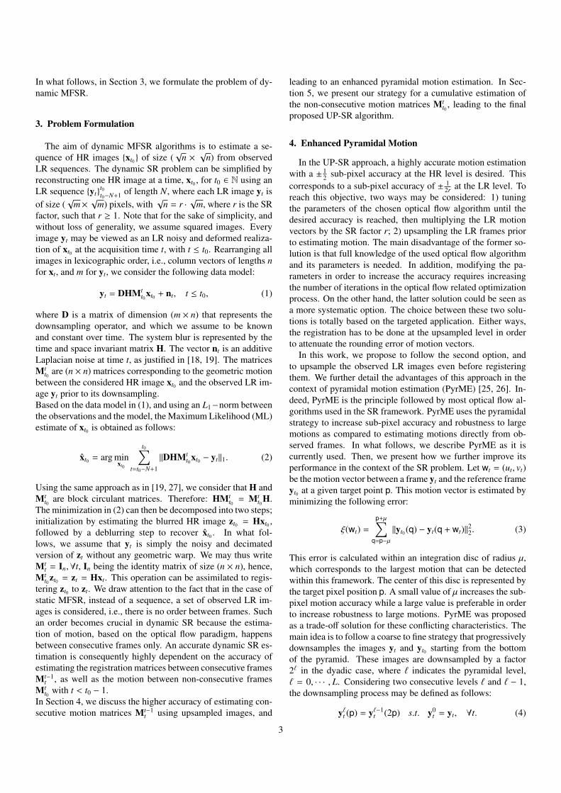
To illustrate the effectiveness of the cumulative registrationproposed in Section 5.2, we consider a challenging case of fourpersons moving with a large motion in different directions. Theused setup is an LR ToF camera, the 3-D MLI [2], mounted inthe ceiling and looking at the scene from the top. One of theLR frames is shown in Figure 2 (a). We apply the UP-SR al-gorithm on this sequence using three different registration tech-niques, namely, non-cumulative registration, cumulative regis-tration using the upscaled motion vectors estimated from LRframes, and the proposed cumulative registration using the es-timated motion from upsampled LR frames. The correspond-ing results are shown in Figure 2 (b), (c), and (d), respectively.They show the superiority of the third technique over the firsttwo techniques, which confirms the advantage of using the pro-posed cumultative motion estimation.

7.3. Qualitative Comparison

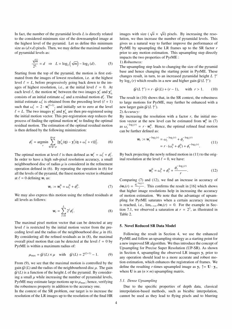
We use the “Samba” dataset available in [40], which pro-vides a real sequence of a 3-D dynamic scene with HR groundtruth, Figure 3 (e). We downsample a sub-sequence of 9 LRframes with a scale factor r = 4. The obtained LR sequenceis of resolution (256 × 147) pixels. This sequence is degradedwith additive Laplacian noise with σ varying from 0 to 100 mm.The created LR noisy depth sequence is then super-resolved. Inorder to visually evaluate the performance of UP-SR, we plotin 3-D the super-resolved results of the “Samba”-generated se-quence for the noise level of σ = 30 mm. As expected, the UP-SR algorithm provides a better result by keeping the fine detailsas compared to the bicubic interpolation and to the patch-basedSISR methods. By zooming on the face part and plotting the3-D error map, it is clear that UP-SR gives the closest result ascompared to the ground truth, see Figure 3 for more details.

Using the same setup of the LR ToF camera mounted in theceiling at a 2.5m height, we captured an LR depth video of twopersons sitting on chairs sliding in two different directions. A

8

(a) (b) (c) (d)

Figure 2: UP-SR results with r = 4 using different registration techniques of a dynamic scene with four persons moving in different directions. The sequenceconsists of 9 LR (56 × 61) depth images. (a) Last frame in the LR sequence. (b) UP-SR without cumulative motion. (c) UP-SR with cumulative motion upscaledfrom LR frames. (d) UP-SR with the proposed cumulative motion from upsampled frames. The largest measured depth in this scene is 2.5 m.

Figure 3: 3-D results of different SR methods applied on the “Samba” sequence [40]. (a) LR noisy input. (b) Bicubic interpolation. (c) Patch-based SISR [12]. (d)UP-SR, initial estimate. (e) Ground truth. (f) Deblurred bicubic. (g) Deblurred patch-based SISR. (h) Deblurred UP-SR. Third row represents the 3-D error mapsfor: (i) Bicubic. (j) Patch-based SISR. (l) Proposed UP-SR. We can see that the obtained error using the the proposed UP-SR (l) is quite small as compared to othermethods where the bicubic interpolation leads to noisy depth measurements in addition to the flying pixels represented by the yellow and orange collors in the 3Derror map in (i). The obtained results using the patch-based SISR is quite smooth and lead to removing fine details, and hence, resulting in large 3-D reconstructionerrors, see blue patches in (j). The depth is measured in mm.

sequence of 9 LR depth images, of size (56×61) pixels, wassuper-resolved with an SR factor r = 5 using bicubic interpo-

lation, 2-D/depth fusion [5], dynamic S&A [41], patch-basedSISR [12], and the proposed UP-SR. Visual results for one

9

(a) (b) (c)

(d) (e) (f)

Figure 4: Moving chairs sequence: comparison of the results for different SR methods with SR factor of r = 5: (a) Last frame of 9 LR (56 × 61) depth images. (b)Bicubic interpolation of the last depth frame in the sequence. (c) 2-D/depth fusion [5]. (d) Dynamic S&A [41]. (e) SISR S&A [12]. (f) Proposed UP-SR.

(a) (b) (c) (d)

Figure 5: Comparison of the results for different SR methods with SR factor of r = 4. These methods are applied on a dynamic sequence of four persons with fastmotion in different directions. (a) Last frame of LR (56 × 61) depth images. (b) Bicubic interpolation of the last depth frame in the sequence. (c) SISR [12]. (d)Proposed UP-SR.

frame are given in Figure 4 (b), (c), (d), (e), and (f), respec-tively. Obtained results show that bicubic interpolation and dy-namic S&A fail on depth data mainly on boundary pixels, whilethe result of the 2-D/depth fusion suffers from strong 2-D tex-ture copying on the final super-resolved depth frame as shownin Figure 4 (c). We can see the results of SISR in Figure 4 (e),where the inaccuracies are also observed especially on objects’boundaries. We show in Figure 4 (f) the result of the UP-SRalgorithm where we obtained clear sharp edges in addition toan efficient removal of noisy pixel values. This is mostly due tothe proposed sub-pixel motion estimation combined with an ac-curate cumulative registration leading to a successful temporalfusion of the sequence. Similar results are observed in Figure 5by testing the different methods on the challenging case of thesequence of four moving persons.

7.4. Quantitative Comparison

We provide a quantitative evaluation of the proposed UP-SRalgorithm as compared to two methods, namely, the conven-tional bicubic interpolation and the patch-based single imageSR (SISR) given in [12]. We start with the ”Samba” dataset,where the previously created LR noisy depth sequences aresuper-resolved using these methods and the proposed method.We compare the obtained results at two levels, initial and de-blurred using the deblurring step proposed in Section 5. Forthe deblurring step we use an exhaustive search to find the bestoptimization parameters corresponding to the smallest 3-D re-construction error. The quantitative results are reported in Fig-ure 6. As expected, by applying the conventional bicubic inter-polation method directly on depth images, a large error in thereconstructed HR depth image is obtained. This error is mainlydue to flying pixels around object’s boundaries, Figure 3 (b).

10

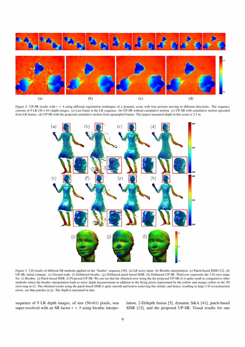
Thus, for a fair comparison we run another round of experi-

Figure 6: MSE at different noise levels for different SR methods applied to anLR depth sequence created from the “Samba” dynamic data [40], with r = 4and N = 9.

ments using a modified bicubic interpolation, where we removeall flying pixels by defining a fixed threshold. Yet, the 3-D re-construction error remains relatively high. This is due to thefact that bicubic interpolation does not profit from the temporalinformation provided by the sequence. Only in the case of onemoving object and a very low noise level (less than 10 mm) themodified bicubic interpolation may be considered as shown bythe red solid line in Figure 6. The performances of SISR, orig-inal and deblurred, are given in green lines, solid, and dashed,respectively. SISR can be seen to be robust to noise as its per-formance is stable even for high noise levels. The addition ofthe deblurring step of UP-SR improves the MSE of the originalSISR algorithm. The result of the proposed UP-SR algorithmis shown with a blue dashed line. Its MSE is the lowest amongall the tested methods, and is also shown to be robust across allnoise levels. This result can be explained by the fact that SISRis a patch-based method where no temporal information is usedin recovering the fine details even after applying a deblurringstep. In contrast, the good quality of the UP-SR results is ob-tained thanks to the temporal fusion using the pixel-wise me-dian filtering after a cumulative registration. This fusion playsa major role in attenuating the temporal noise and represents anappropriate process to deal with the problem of flying pixels.Moreover, the spatial deblurring step leads to further adding asmoothing effect while keeping sharp edges, hence, recoveringfine details.

7.5. Evaluation for Varying SR Factors

In order to evaluate the performance of the proposed UP-SRalgorithm for different SR factors and varying noise levels, ascompared to the statistical performance analysis of Section 6,we setup the following experiment. We use the publiclyavailable toolbox V-REP [42] to create synthetic data withfully known ground truth of a laterally moving person withless complex motions as compared to the “Samba” dataset.Three depth cameras with the same field of view are fixed atthe same position. These cameras are of different resolutions,namely, 5122, 2562, and 1282 pixels. They are used to capturethree sequences of the moving person. These sequences are

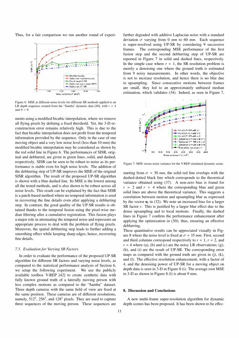
further degraded with additive Laplacian noise with a standarddeviation σ varying from 0 mm to 60 mm. Each sequenceis super-resolved using UP-SR by considering 9 successiveframes. The corresponding MSE performance of the firstfusion step and the second deblurring step of UP-SR arereported in Figure 7 in solid and dashed lines, respectively.In the simple case where r = 1, the SR resolution problem ismerely a denoising one where the ground truth is estimatedfrom 9 noisy measurements. In other words, the objectiveis not to increase resolution, and hence there is no blur dueto upsampling. Since consecutive motions between framesare small, they led to an approximately unbiased medianestimation, which validates (34). Indeed, as seen in Figure 7,

Figure 7: MSE versus noise variance for the V-REP simulated dynamic scene.

starting from σ ≈ 30 mm, the solid red line overlaps with thedashed-dotted black line which corresponds to the theoreticalvariance obtained using (37). A non-zero bias is found forr = 2 and r = 4 where the corresponding blue and greensolid lines are above the theoretical variance. This suggests acorrelation between motion and upsampling blur as expressedby the vector ui in (32). We note an increased bias for a largerSR factor r. This is justified by a larger blur effect due to thedense upsampling and to local motions. Finally, the dashedlines in Figure 7 confirm the performance enhancement afterapplying the optimization in (30); thus, ensuring an effectivedeblurring.These quantitative results can be appreciated visually in Fig-ure 8 where the noise level is fixed at σ = 35 mm. First, secondand third columns correspond respectively to r = 1, r = 2, andr = 4 where (a), (b) and (c) are the noisy LR observations; (g),(h), and (i) are the result of UP-SR. The corresponding errormaps as compared with the ground truth are given in (j), (k),and (l). The effective resolution enhancement, with a factor of4, and the denoising power of UP-SR for a moving object ondepth data is seen in 3-D in Figure 8 (i). The average root MSEin 3-D as shown in Figure 8 (l) is about 9 mm.

8. Discussion and Conclusions

A new multi-frame super-resolution algorithm for dynamicdepth scenes has been proposed. It has been shown to be effec-

11

Figure 8: UP-SR qualitative results for the V-REP simulated moving personwith different SR factors r. First, second and third columns correspond respec-tively to r = 1, r = 2, and r = 4 where (a), (b) and (c) are the noisy LR observa-tions; (d), (e), and (f) are the result of the initialization step of UP-SR; (g), (h),and (i) are the result of the deblurring step of UP-SR. The corresponding errormaps as compared to the ground truth are given in (j), (k), and (l)

tive in enhancing the resolution of dynamic scenes with one ormultiple non-rigidly moving objects. The proposed algorithmrelies on two main components; first, an enhanced motion es-timation based on a prior upsampling of the observed low res-olution depth frames up to the super-resolution factor. Second,it uses a cumulative motion estimation accurately relating non-consecutive frames in the considered depth sequence, even forrelatively large motions. In addition, the multi-frame super-resolution problem has been reformulated defining a simplifieddata model which is analogous to a classical image denoisingproblem with additive Laplacian noise, and using multiple ob-servations. This has led to a median initial estimate, further re-fined by a deblurring operation using a bilateral total variationas the regularization term. For a thorough understanding of theimpact of the different parameters, namely, number of observedframes N and the super-resolution factor r, a statistical modelfor the proposed approach in terms of MSE has been derived.One important conclusion is that the blur effect is due to bothupsampling, motion and occlusions. Extensive evaluations us-ing synthetic and real data have been carried out, showing theconsistent good performance of the proposed approach in fullcorrespondence with the derived theoretical statistical model.We note, nevertheless, interesting limitations in the case, forexample, of intersecting or touching objects, as can be seenwithin the bounding boxes in Figure 2 (d) and Figure 5 (d).This is due to the textureless nature of depth images which maycause two objects to be allocated to the same depth value, andhence makes them wrongly appear as one object. In the future,

we will consider a full 3-D motion for a more accurate registra-tion that should solve such ambiguous cases. Furthermore, weplan to investigate recursive approaches for a real time dynamicdepth super-resolution. The results of this work are very novelas compared to state-of-art multi-frame super-resolution tech-niques applied to depth data. They are expected to have a sig-nificant impact in increasing the deployment of cost-effectivelow resolution depth cameras in many applications, such as,robotics, gaming, and security.

Appendix A. Proof of the Cumulative Motion Estimation

We prove by induction the following ζ(n) statement:{Mt0

t0−nyt0−n ↑ = yt0t0−n ↑,

s.t. Mt0t0−n = Mt0

t0−1Mt0−1t0−2...M

t0−n+1t0−n

· · · ζ(n).

Proof. Let us consider that ζ(n − 1) is true, i.e. Mt0t0−(n−1)yt0−(n−1) ↑ = yt0

t0−(n−1) ↑,

s.t. Mt0t0−(n−1) = Mt0

t0−1Mt0−1t0−2...M

t0−(n−1)+1t0−(n−1)

(A.1)

From (A.1) we have:

Mt0t0−(n−1)M

t0−(n−1)t0−n = Mt0

t0−n (A.2)

Base case: When n = 1 we have

Mt0t0 yt0 ↑= yt0

t0 ↑, (A.3)

and

Mt0t0 Mt0−1

t0 = Mt0−1t0 . (A.4)

Both (A.3) and (A.4) are verified because Mt0t0 = In. Then,

Induction step: We need to show that ζ(n − 1)⇒ ζ(n).Given two consecutive frames: yt0−n and yt0−(n−1), we have:

Mt0−(n−1)t0−n yt0−n ↑= yt0−(n−1)

t0−n ↑, (A.5)

where

Mt0−(n−1)t0−n = arg min

MΨ

(yt0−(n−1) ↑, yt0−n ↑,M

). (A.6)

Multiplying (A.5) by Mt0t0−(n−1) we find

Mt0t0−(n−1)M

t0−(n−1)t0−n yt0−n ↑= Mt0

t0−(n−1)yt0−(n−1)t0−n ↑ . (A.7)

From (A.2) and (A.7) we have

Mt0t0−nyt0−n ↑= yt0

t0−n ↑ .

[1] M. Lindner, A. Kolb, “Compensation of motion artifacts for timeof-flightcameras,” in Proc. Dynamic 3D Vision Workshop, vol. 5742, Jena, Sep.2009, pp. 1627.

[2] 3D MLI, 2015, http://www.iee.lu/home-page.[3] pmd CamBoard nano, 2015, http://www.pmdtec.com/products ser-

vices/reference design.php.

12

[4] Q. Yang, R. Yang, J. Davis, D. Nister, “Spatial-Depth Super Resolutionfor Range Images,” IEEE Int. Conf. Computer Vision and Pattern Recog-nition, vol., pp. 1-8 2007.

[5] F. Garcia, D. Aouada, B. Mirbach, T. Solignac, B. Ottersten, “Real-timeHybrid ToF Multi-Camera Rig Fusion System for Depth Map Enhance-ment,” IEEE Int. Conf. Computer Vision and Pattern Recognition Work-shops, vol., pp. 1-8, 2011.

[6] J. Zhu, L. Wang, R. Yang, and J. Davis, “Fusion of time-of-flight depthand stereo for high accuracy depth maps,” IEEE Int. Conf. Computer Vi-sion and Pattern Recognition, vol., pp. 1-8, 2008.

[7] Q. Yang, K. Tan, B. Culbertson, J. Apostolopoulos, “Fusion of Active andPassive Sensors for Fast 3D Capture,” IEEE Int. Workshops MultimediaSignal Processing, vol., pp. 69-74, 2010.

[8] “Super-Resolution Imaging”, by Peyman Milanfar, in CRC Press, 2010.[9] S. Schuon, C. Theobalt, J. Davis, and S. Thrun, “High-quality scanning

using time-of-flight depth superresolution,” IEEE Computer Vision andPattern Recognition Workshops, vol., pp. 1-7, 2008.

[10] S. Schuon, C. Theobalt, J. Davis, S. Thrun, “LidarBoost: Depth super-resolution for ToF 3D shape scanning,” IEEE Int. Conf. Computer Visionand Pattern Recognition., vol., pp.343-350, 2009.

[11] Y. Cui, S. Schuon, S. Thrun, D. Stricker, C. Theobalt, “Algorithms for 3DShape Scanning with a Depth Camera,” IEEE Trans. on Pattern Analysisand Machine Intelligence., vol.35, pp. 1039-1050, 2013.

[12] O. M. Aodha, N. Campbell, A. Nair, G. Brostow, “Patch Based Synthesisfor Single Depth Image Super-Resolution,” European Conf. on ComputerVision., vol. Part III, pp. 71-84, 2012.

[13] K. Al Ismaeil, D. Aouada, B. Mirbach, B. Ottersten, “Dynamic Super-Resolution of Depth Sequences with Non-Rigid Motions,” IEEE Int.Conf. Image processing., vol., pp. 660-664, 2013.

[14] K. Al Ismaeil, D. Aouada, B. Mirbach, B. Ottersten, “Multi-Frame Super-Resolution by Enhanced Shift & Add”, IEEE Int. Symposium on Imageand Signal Processing and Analysis., vol., pp. 171-176, 2013.

[15] D. Aouada, K. Al Ismaeil, B. Ottersten, “Patch-based Statistical Perfor-mance Analysis of Upsampling for Precise SuperResolution,” Int. Conf.on Computer Vision Theory and Applications, 2015.

[16] L. Xu, J. Jia, S. B. Kang, “Improving sub-pixel correspondence throughupsampling,” Journal on Computer Vision and Image Understanding.,vol. 116, pp. 250-261, 2012.

[17] S. D. Babacan, R. Molina, and A.K. Katsaggelos. “Variational BayesianSuper Resolution”. IEEE Trans. Image Process., vol. 20, pp. 984-999,2011.

[18] S. Farsiu, D. Robinson, M. Elad, P. Milanfar, “Robust Shift and AddApproach to Super-Resolution,” Int. Symposium on Optical Science andTechnology., vol. 5203, pp.121-130, 2003.

[19] S. Farsiu, D. Robinson, M. Elad, and P. Milanfar, “Fast and Robust Multi-Frame Super-Resolution,” IEEE Trans. Image Process., vol. 13, pp. 1327-1344, 2004.

[20] K. Al Ismaeil, D. Aouada, B. Mirbach, B. Ottersten, “Bilateral FilterEvaluation Based on Exponential Kernels,” Int. Conf. on Pattern Recog-nition, pp. 258-261, 2012.

[21] R. Hardie, T. Tuinstra, K. Barnard, J. Bognar, and E. Armstrong, “Highresolution image reconstruction from digital video with global and non-global scene motion.” IEEE Int. Conf. Image Process., vol. 1, pp. 153-156, 1997.

[22] S. Farsiu, M. Elad, adn P. Milanfar, “Video-to-Video Dynamic Superreso-lution for Grayscale and Color Sequences,” Journal on Advances in SignalProcessing., 2006.

[23] A. W. M. van Eekeren, K. Schutte, J. Dijk, Dirk-Jan de Lange, and L. J.van Vliet, “Super-Resolution on Moving Objects and Background,” IEEEInt. Conf. Image Process., vol., pp. 2709-2712, 2006.

[24] A. W. M. van Eekeren, K. Schutte, and L. J. van Vliet, “Multiframe Super-Resolution Reconstruction of Small Moving Objects,” IEEE Trans. onImage Process., vol. 19, pp. 2901-2912, 2010.

[25] J. Y. Bouguet, “Pyramidal implementation of the LukasKanade feature tracker. Description of the algorithm”.http://robots.stanford.edu/cs223b04/algo tracking.

[26] J. R. Bergen, P. Anandan, K. J. Hanna, and R. Hingorani. “ HierarchicalModel-Based Motion Estimation,” European Conf. on Computer Vision.,vol. 588, pp. 237-252, 1992.

[27] H. Takeda, P. Milanfar, M. Protter, and M. Elad, “Superresolution withoutExplicit Subpixel Motion Estimation,” IEEE Trans. on Image Process.,

vol. 18, pp. 1958-1975, 2009.[28] F. Garcia, D. Aouada, B. Mirbach, T. Solignac, B. Ottersten, “Spatio-

Temporal ToF Data Enhancement by Fusion,” IEEE Int. Conf. Image Pro-cess., vol., pp. 981-984, 2012.

[29] M. Elad and A. Feuer, “Super-Resolution reconstruction of ContinuousImage Sequence,” IEEE Trans. on Pattern Analysis and Machine Intelli-gence., Vol. 21, No. 9, pp. 817-834, 1999.

[30] D. Chan, H. Buisman, C. Theobalt, S. Thrun, “A Noise-Aware Filter forReal-Time Depth Upsampling”, Workshop on Multi-camera and Multi-modal Sensor Fusion, 2008.

[31] A. Zomet, A. Rav-Acha, and S. Peleg, “Robust Super-Resolution,” IEEEInt. Conf. on Computer Vision and Pattern Recognition., vol. 1, pp. 645-650, 2001.

[32] Richard A. Newcombe, Shahram Izadi, Otmar Hilliges, DavidMolyneaux, David Kim, Andrew J. Davison, Pushmeet Kohli, JamieShotton, Steve Hodges, Andrew Fitzgibbon, “KinectFusion: Real-TimeDense Surface Mapping and Tracking”, IEEE ISMAR, October 2011.

[33] K. Al Ismaeil, D. Aouada, B. Mirbach, B. Ottersten, “Depth Super-Resolution by Enhanced Shift and Add,” 15th International Conferencein Computer Analysis of Images and Patterns, 2013.

[34] A. Rajagopalan and P. Kiran, “Motion-free superresolution and the roleof relative blur,” J. Opt. Soc. Amer., vol. 20, pp. 20222032, 2003.

[35] D. Robinson, and P. Milanfar, “Statistical Performance Analysis of Super-resolution,” IEEE Trans. on Image Processing., Vol. 15, pp. 1413-1428,2006.

[36] Robinson and Milanfar, “Bias-minimizing filters for motion estimation,”IEEE Asilomar Conf. on Signals, Systems and Computers., 2003.

[37] P. Chatterjee and P. Milanfar, “Bias modeling for image denoising,” IEEEAsilomar Conf. on Signals, Systems and Computers., vol., pp.856-859,2009.

[38] N.C. Beaulieu and S. Jiang, “ML estimation of signal amplitude inLaplace noise,” IEEE Conf. Global Telecommunications., vol., pp. 1-5,2010.

[39] http://vision.middlebury.edu/stereo/data/

[40] http://people.csail.mit.edu/drdaniel/mesh animation/

[41] S. Farsiu, D. Robinson, M. Elad, and P. Milanfar, “Advances and Chal-lenges in Super-Resolution,” Int. Journal of Imaging Systems and Tech-nology, vol. 14, pp. 47-57, 2004.

[42] http://www.k-team.com/mobile-robotics-products/v-rep

13