1

ISSN 2346-4119

Engineering Seismology

Dr. S.K. Sarma

Civil Engineering Department

Imperial College of Science,Technology & Medicine

London SW7 2BU

Tel: 0207 594 6054

Fax: 0207 225 2716

email: s.sarma@ic.ac.uk

September 2013

2

1. Engineering Seismology

Engineering Seismology is the study of Seismology as related to Engineering. This involves

understanding the source, the size and the mechanisms of earthquakes, how the ground

motion propagates from the source to the site of engineering importance, the characteristics

of ground motion at the site and how the ground motion is evaluated for engineering design.

This subject is therefore related to the hazard of earthquakes. The seismic hazard at a site

cannot be controlled. It can only be assessed. In the same context, Earthquake Engineering

is the subject of analysis and design of structures to resist stresses caused by the earthquake

ground motion. Resisting the stresses imply either resisting without failure or yielding to the

stresses gracefully without collapse. This subject is related to the vulnerability of built

structures to seismic ground motion. The vulnerability is controlled by design. The decision

to control the vulnerability of a structure is based on the economics of the situation and on the

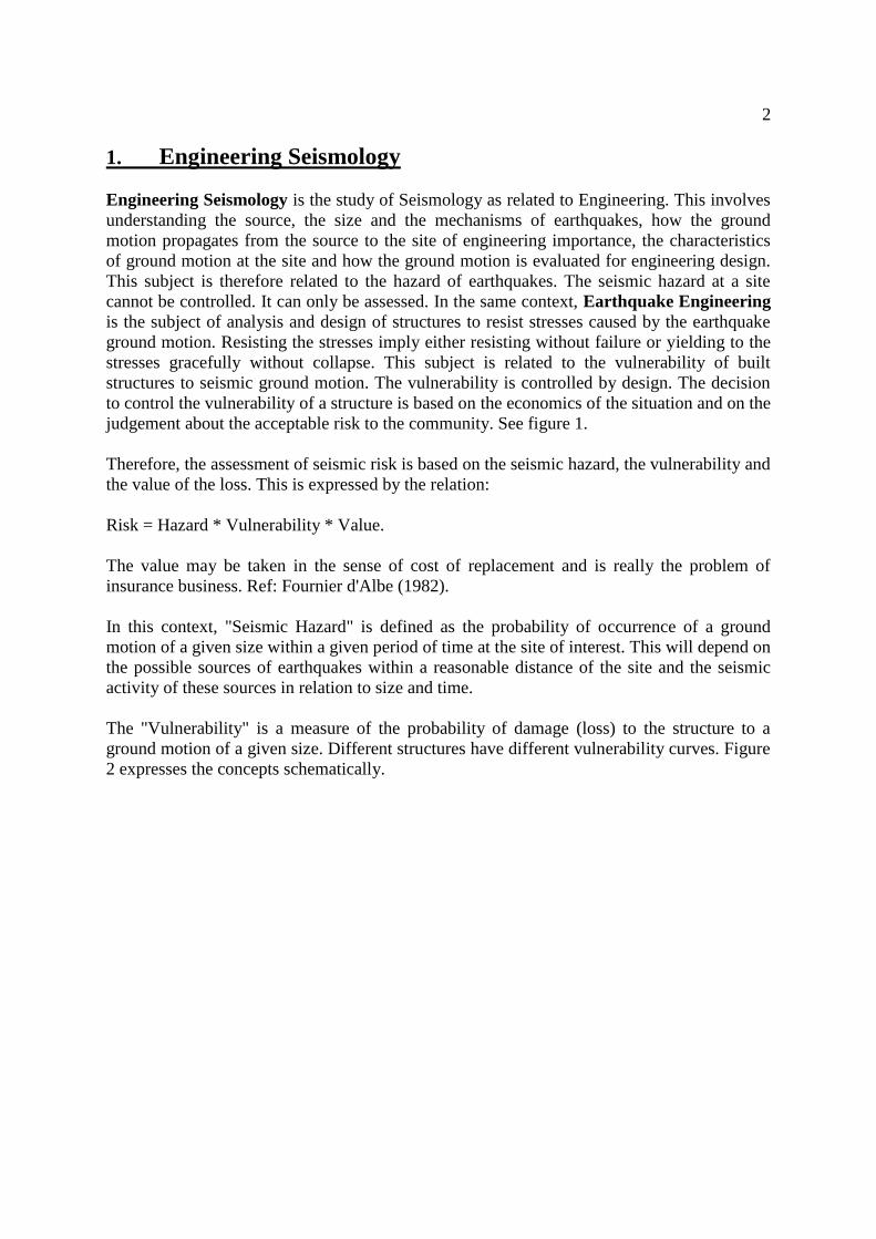
judgement about the acceptable risk to the community. See figure 1.

Therefore, the assessment of seismic risk is based on the seismic hazard, the vulnerability and

the value of the loss. This is expressed by the relation:

Risk = Hazard * Vulnerability * Value.

The value may be taken in the sense of cost of replacement and is really the problem of

insurance business. Ref: Fournier d'Albe (1982).

In this context, "Seismic Hazard" is defined as the probability of occurrence of a ground

motion of a given size within a given period of time at the site of interest. This will depend on

the possible sources of earthquakes within a reasonable distance of the site and the seismic

activity of these sources in relation to size and time.

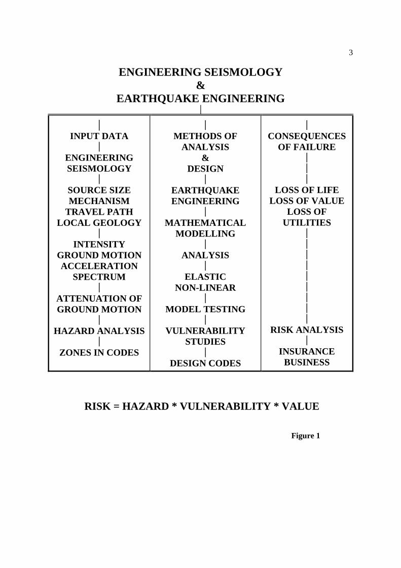
The "Vulnerability" is a measure of the probability of damage (loss) to the structure to a

ground motion of a given size. Different structures have different vulnerability curves. Figure

2 expresses the concepts schematically.

3

ENGINEERING SEISMOLOGY

&

EARTHQUAKE ENGINEERING

│

│

INPUT DATA │

ENGINEERING

SEISMOLOGY │

SOURCE SIZE

MECHANISM

TRAVEL PATH

LOCAL GEOLOGY │

INTENSITY

GROUND MOTION

ACCELERATION

SPECTRUM │

ATTENUATION OF

GROUND MOTION │

HAZARD ANALYSIS │

ZONES IN CODES

│

METHODS OF

ANALYSIS

&

DESIGN │

EARTHQUAKE

ENGINEERING │

MATHEMATICAL

MODELLING │

ANALYSIS │

ELASTIC

NON-LINEAR │

MODEL TESTING │

VULNERABILITY

STUDIES │

DESIGN CODES

│

CONSEQUENCES

OF FAILURE │

│

│

LOSS OF LIFE

LOSS OF VALUE

LOSS OF

UTILITIES │

│

│

│

│

│

│

│

│

RISK ANALYSIS │

INSURANCE

BUSINESS

RISK = HAZARD * VULNERABILITY * VALUE

Figure 1

4

Seismicity and Plate tectonics:

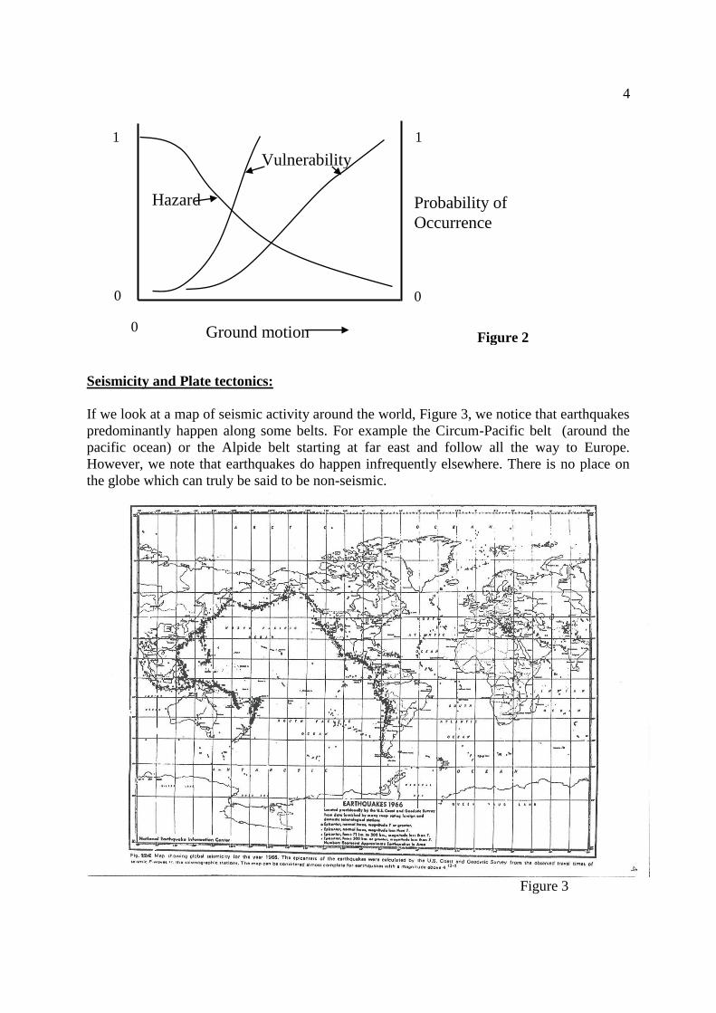
If we look at a map of seismic activity around the world, Figure 3, we notice that earthquakes

predominantly happen along some belts. For example the Circum-Pacific belt (around the

pacific ocean) or the Alpide belt starting at far east and follow all the way to Europe.

However, we note that earthquakes do happen infrequently elsewhere. There is no place on

the globe which can truly be said to be non-seismic.

Figure 3

Probability of

Occurrence

1 1

Ground motion

0 0

Hazard

Vulnerability

0 Figure 2

5

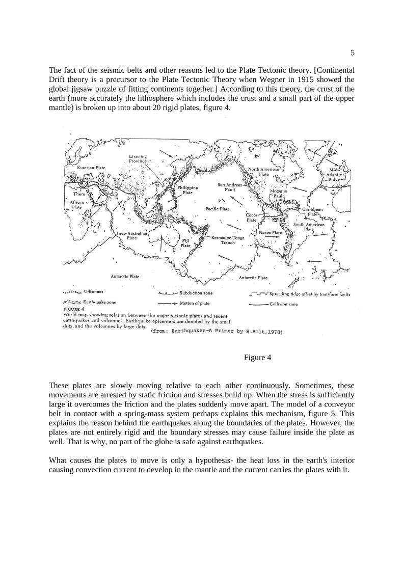
The fact of the seismic belts and other reasons led to the Plate Tectonic theory. [Continental

Drift theory is a precursor to the Plate Tectonic Theory when Wegner in 1915 showed the

global jigsaw puzzle of fitting continents together.] According to this theory, the crust of the

earth (more accurately the lithosphere which includes the crust and a small part of the upper

mantle) is broken up into about 20 rigid plates, figure 4.

Figure 4

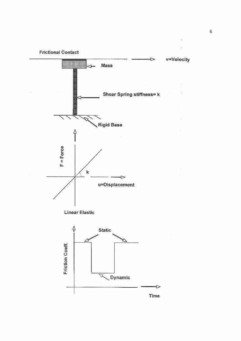
These plates are slowly moving relative to each other continuously. Sometimes, these

movements are arrested by static friction and stresses build up. When the stress is sufficiently

large it overcomes the friction and the plates suddenly move apart. The model of a conveyor

belt in contact with a spring-mass system perhaps explains this mechanism, figure 5. This

explains the reason behind the earthquakes along the boundaries of the plates. However, the

plates are not entirely rigid and the boundary stresses may cause failure inside the plate as

well. That is why, no part of the globe is safe against earthquakes.

What causes the plates to move is only a hypothesis- the heat loss in the earth's interior

causing convection current to develop in the mantle and the current carries the plates with it.

6

7

Figure 5

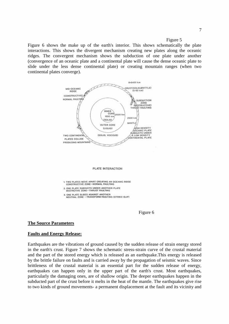
Figure 6 shows the make up of the earth's interior. This shows schematically the plate

interactions. This shows the divergent mechanism creating new plates along the oceanic

ridges. The convergent mechanism shows the subduction of one plate under another

(convergence of an oceanic plate and a continental plate will cause the dense oceanic plate to

slide under the less dense continental plate) or creating mountain ranges (when two

continental plates converge).

Figure 6

The Source Parameters

Faults and Energy Release:

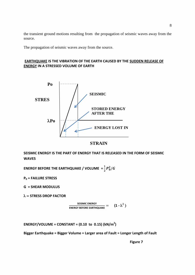
Earthquakes are the vibrations of ground caused by the sudden release of strain energy stored

in the earth's crust. Figure 7 shows the schematic stress-strain curve of the crustal material

and the part of the stored energy which is released as an earthquake.This energy is released

by the brittle failure on faults and is carried away by the propagation of seismic waves. Since

brittleness of the crustal material is an essential part for the sudden release of energy,

earthquakes can happen only in the upper part of the earth's crust. Most earthquakes,

particularly the damaging ones, are of shallow origin. The deeper earthquakes happen in the

subducted part of the crust before it melts in the heat of the mantle. The earthquakes give rise

to two kinds of ground movements- a permanent displacement at the fault and its vicinity and

8

the transient ground motions resulting from the propagation of seismic waves away from the

source.

The propagation of seismic waves away from the source.

EARTHQUAKE IS THE VIBRATION OF THE EARTH CAUSED BY THE SUDDEN RELEASE OF ENERGY IN A STRESSED VOLUME OF EARTH

SEISMIC ENERGY IS THE PART OF ENERGY THAT IS RELEASED IN THE FORM OF SEISMIC

WAVES

ENERGY BEFORE THE EARTHQUAKE / VOLUME =

P0 = FAILURE STRESS

G = SHEAR MODULUS

STRESS DROP FACTOR

(1 -

ENERGY/VOLUME = CONSTANT = (0.10 to 0.15) (kN/m2)

Bigger Earthquake = Bigger Volume = Larger area of Fault = Longer Length of Fault

Figure 7

Po

Po

STRES

S

STRAIN

SEISMIC

ENERGY

STORED ENERGY

AFTER THE

EARTHQUAKE

ENERGY LOST IN

HEAT

9

Elastic strain energy builds up on a fault, which is held static by friction, until the stresses

overcome the strength and slip is initiated. Since nature favours an existing fault (finds it

easier to break) than a new one, the same faults move repeatedly in successive earthquakes.

This does not mean that new faults cannot ever be generated and therefore, theoretically, no

part on earth is ever safe from earthquakes

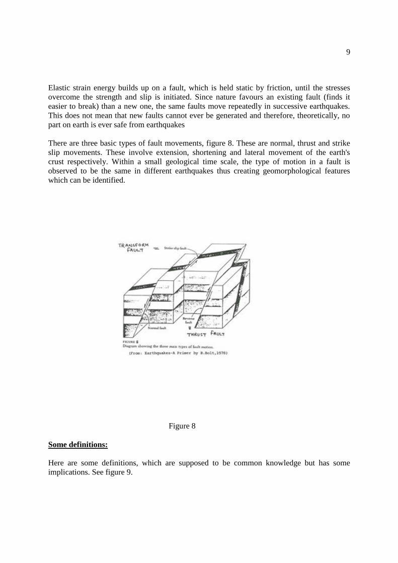
There are three basic types of fault movements, figure 8. These are normal, thrust and strike

slip movements. These involve extension, shortening and lateral movement of the earth's

crust respectively. Within a small geological time scale, the type of motion in a fault is

observed to be the same in different earthquakes thus creating geomorphological features

which can be identified.

Figure 8

Some definitions:

Here are some definitions, which are supposed to be common knowledge but has some

implications. See figure 9.

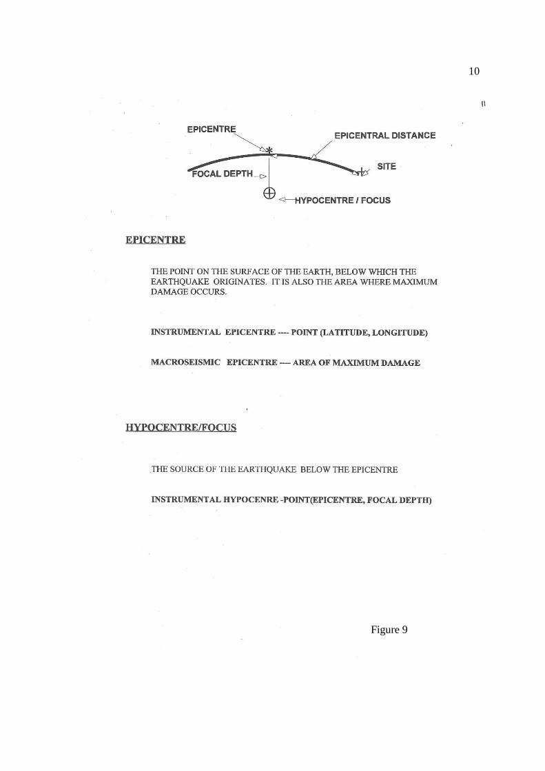
10

Figure 9

11

Hypocentre or Focus:

The point on the fault where slip is first originated. From this point, the slip propagates and

spreads over the rupture surface (the fault) until the slip is stopped by either strong material

or less stress. The hypocentre is represented by three coordinates: Latitude, Longitude and the

depth from the earth's surface. Note that the whole fault does not move at the same instant.

Epicentre:

The point on the earth's surface immediately above the hypocentre. It is represented by the

latitude and longitude of the point. The error in the determination of the epicentre is about

10km presently. But in the old days, this error could be very large. There are instances of the

determination in the wrong hemisphere. It is therefore essential to correlate the instrumental

determination of epicentre with the area of maximum damage.

Focal depth:

This is the depth of focus below the epicentre. There are three grades of depth- Shallow,

Intermediate and Deep. Most continental earthquakes are shallow and these are of

engineering importance. Focal depth of an earthquake is the most difficult one to determine

and should be treated with caution. In the bulletin of earthquakes, most earthquakes are given

a focal depth of 33km which simply imply that these are of shallow depth but the depth was

not possible to determine any more accurately.

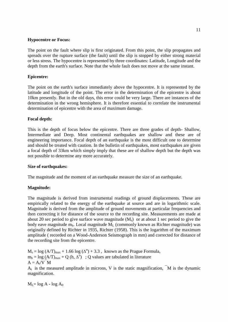
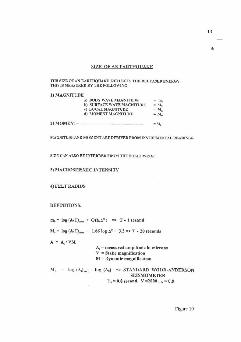
Size of earthquakes:

The magnitude and the moment of an earthquake measure the size of an earthquake.

Magnitude:

The magnitude is derived from instrumental readings of ground displacements. These are

empirically related to the energy of the earthquake at source and are in logarithmic scale.

Magnitude is derived from the amplitude of ground movements at particular frequencies and

then correcting it for distance of the source to the recording site. Measurements are made at

about 20 sec period to give surface wave magnitude (Ms) or at about 1 sec period to give the

body eave magnitude mb. Local magnitude ML (commonly known as Richter magnitude) was

originally defined by Richter in 1935, Richter (1958). This is the logarithm of the maximum

amplitude ( recorded on a Wood-Anderson Seismograph in mm) and corrected for distance of

the recording site from the epicentre.

Ms = log (A/T)max + 1.66 log (o) + 3.3 , known as the Prague Formula,

mb = log (A/T)max + Q (h, o) ; Q values are tabulated in literature

A = At/VM

At is the measured amplitude in microns, V is the static magnification, M is the dynamic

magnification.

ML= log A - log A0

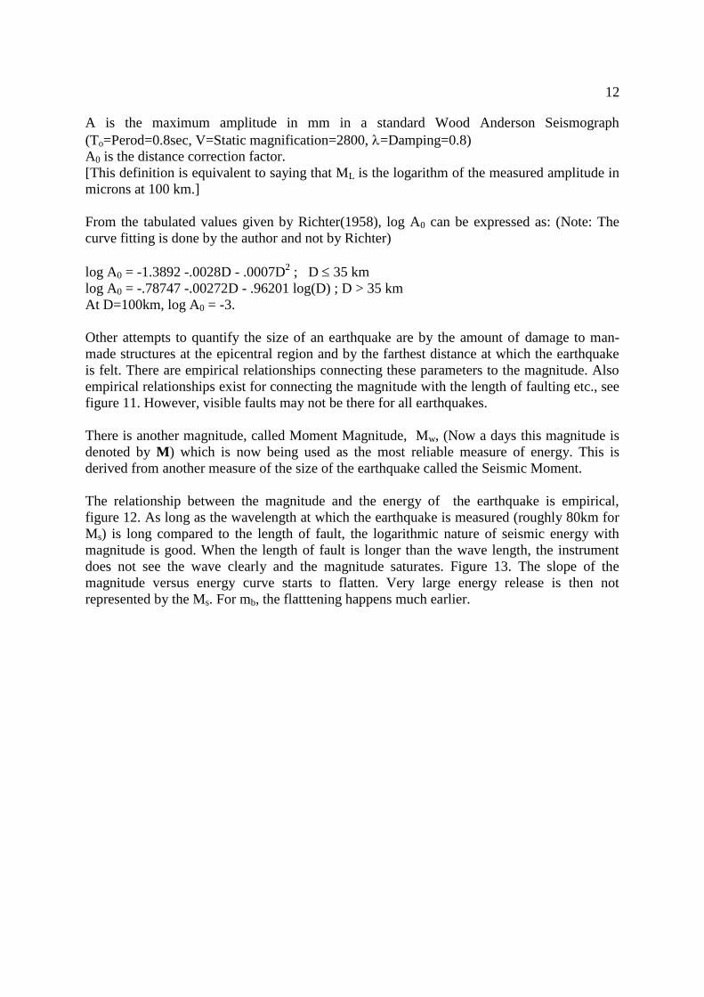
12

A is the maximum amplitude in mm in a standard Wood Anderson Seismograph

(To=Perod=0.8sec, V=Static magnification=2800, =Damping=0.8)

A0 is the distance correction factor.

[This definition is equivalent to saying that ML is the logarithm of the measured amplitude in

microns at 100 km.]

From the tabulated values given by Richter(1958), log A0 can be expressed as: (Note: The

curve fitting is done by the author and not by Richter)

log A0 = -1.3892 -.0028D - .0007D2 ; D 35 km

log A0 = -.78747 -.00272D - .96201 log(D) ; D > 35 km

At D=100km, log A0 = -3.

Other attempts to quantify the size of an earthquake are by the amount of damage to man-

made structures at the epicentral region and by the farthest distance at which the earthquake

is felt. There are empirical relationships connecting these parameters to the magnitude. Also

empirical relationships exist for connecting the magnitude with the length of faulting etc., see

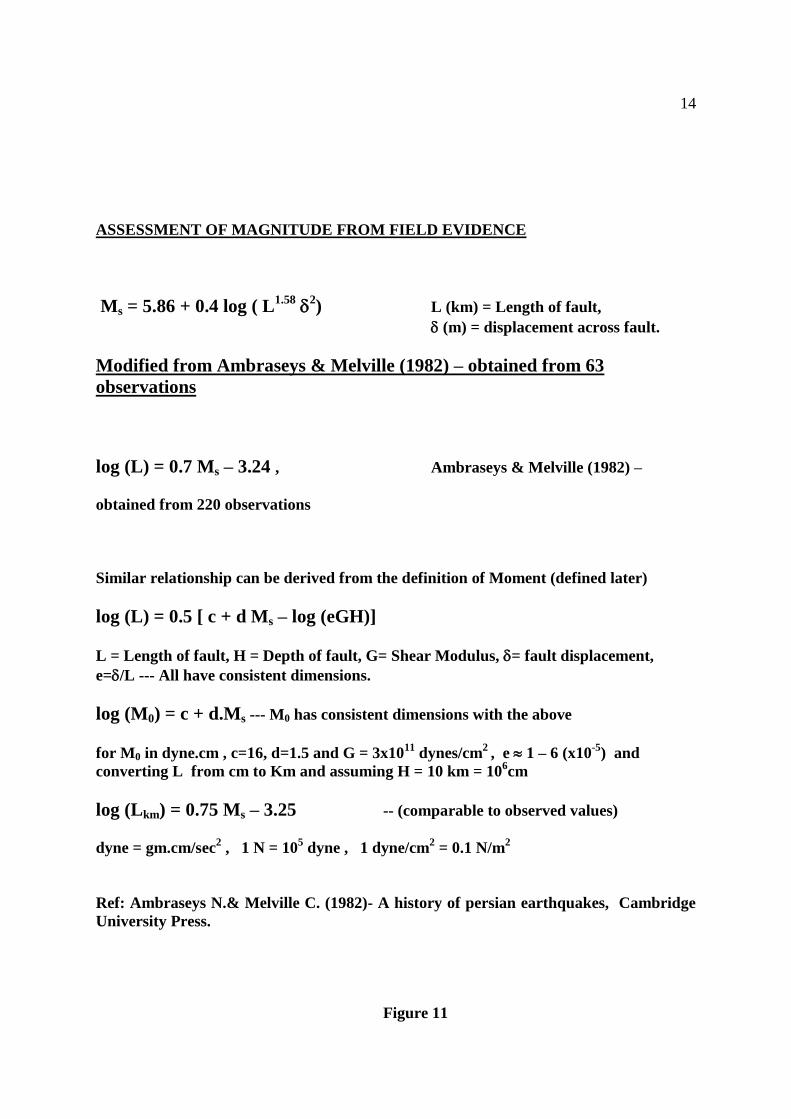
figure 11. However, visible faults may not be there for all earthquakes.

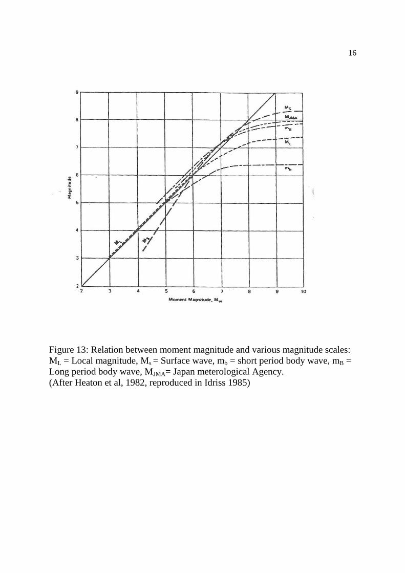
There is another magnitude, called Moment Magnitude, Mw, (Now a days this magnitude is

denoted by M) which is now being used as the most reliable measure of energy. This is

derived from another measure of the size of the earthquake called the Seismic Moment.

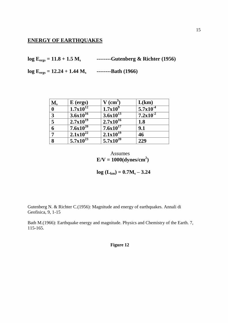
The relationship between the magnitude and the energy of the earthquake is empirical,

figure 12. As long as the wavelength at which the earthquake is measured (roughly 80km for

Ms) is long compared to the length of fault, the logarithmic nature of seismic energy with

magnitude is good. When the length of fault is longer than the wave length, the instrument

does not see the wave clearly and the magnitude saturates. Figure 13. The slope of the

magnitude versus energy curve starts to flatten. Very large energy release is then not

represented by the Ms. For mb, the flatttening happens much earlier.

13

Figure 10

14

ASSESSMENT OF MAGNITUDE FROM FIELD EVIDENCE

Ms = 5.86 + 0.4 log ( L1.58

2) L (km) = Length of fault,

(m) = displacement across fault.

Modified from Ambraseys & Melville (1982) – obtained from 63

observations

log (L) = 0.7 Ms – 3.24 , Ambraseys & Melville (1982) –

obtained from 220 observations

Similar relationship can be derived from the definition of Moment (defined later)

log (L) = 0.5 [ c + d Ms – log (eGH)]

L = Length of fault, H = Depth of fault, G= Shear Modulus, = fault displacement,

e=/L --- All have consistent dimensions.

log (M0) = c + d.Ms --- M0 has consistent dimensions with the above

for M0 in dyne.cm , c=16, d=1.5 and G = 3x1011

dynes/cm2

, e 1 – 6 (x10-5

) and

converting L from cm to Km and assuming H = 10 km = 106cm

log (Lkm) = 0.75 Ms – 3.25 -- (comparable to observed values)

dyne = gm.cm/sec2 , 1 N = 10

5 dyne , 1 dyne/cm

2 = 0.1 N/m

2

Ref: Ambraseys N.& Melville C. (1982)- A history of persian earthquakes, Cambridge

University Press.

Figure 11

15

ENERGY OF EARTHQUAKES

log Eergs = 11.8 + 1.5 Ms --------Gutenberg & Richter (1956)

log Eergs = 12.24 + 1.44 Ms --------Bath (1966)

s E (ergs) V (cm3) L(km)

0 1.7x1012

1.7x109

5.7x10-4

3 3.6x1016

3.6x1013

7.2x10-2

5 2.7x1019

2.7x1016

1.8

6 7.6x1020

7.6x1017

9.1

7 2.1x1022

2.1x1019

46

8 5.7x1023

5.7x1020

229

Assumes

E/V = 1000(dynes/cm2)

log (Lkm) = 0.7Ms – 3.24

Gutenberg N. & Richter C.(1956): Magnitude and energy of earthquakes. Annali di

Geofisica, 9, 1-15

Bath M.(1966): Earthquake energy and magnitude. Physics and Chemistry of the Earth. 7,

115-165.

Figure 12

16

Figure 13: Relation between moment magnitude and various magnitude scales:

ML = Local magnitude, Ms = Surface wave, mb = short period body wave, mB =

Long period body wave, MJMA= Japan meterological Agency.

(After Heaton et al, 1982, reproduced in Idriss 1985)

17

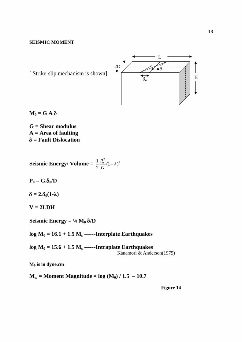
Seismic Moment:

Seismic moment is defined as the following: See figure 14.

M0 = A u

is the shear modulus of the medium (3x1010

N/m2), A is the fault area (m

2) and u is the

vector displacement (m) of one side of the fault relative to the other. M0 has the dimension of

(Nm).

M0 can be calculated from direct measurement in the field if available. This can also be

measured from the long period level of the seismic spectrum. Observations from large

earthquake show that the fault displacement has a consistent ratio to the fault length (1-6 x10-

5).

There are relationships linking the moment M0 to the magnitude Ms . Hanks & Kanamori

(1979) gives:

log M0 = 1.5 Ms + 16.1 ; In this formula, M0 is in dyne.cm . [ 1Nm=107 dyne.cm ]

[ Note that the inversion of this formula defines Mw]

The linear relationship between log M0 and Ms does not seem to be true for smaller

magnitudes. Other non-linear relationships exist, for example, Ekstrom & Dziewonski (1988)

and Ambraseys & Free (1997).

We can use these relationships to estimate the maximum possible magnitude in a fault or

estimate the permanent fault displacements in a major earthquake in the fault. For example: If

a capable fault exists which is say 200 km long and 10 km deep (Anatolian fault for

example), the estimated maximum fault displacement can be of the order of 5x10-5

L which

will be about 10m. The moment M0 for this earthquake will be:

M0 = 3.3x1010

(200x10x106)x10 Nm=6.6x10

20 Nm =6.6x10

27dyne.cm.

This will then convert to Ms = 7.8. Thus, on a fault of the size of 200km, 7.8 magnitude

earthquake may be expected.

Similarly, we may estimate the fault displacements for earthquakes of various magnitudes.

We can see that displacements across faults for a medium size earthquake, say of magnitude

Ms=6 may be of the order of a meter. Using log(Lkm)=0.7Ms -3.24 will give u = 0.47m. Thus,

if we are considering a dam across a fault and the design earthquake is a magnitude 6 one,

then the design must consider a possible fault movement of 1/2 metre. Note that rivers may

be fault alignments and this is a serious concern in dam engineering. A proper site

investigation looking for faults is a must in any dam engineering.

18

SEISMIC MOMENT

[ Strike-slip mechanism is shown]

M0 = G A

G = Shear modulus

A = Area of faulting

= Fault Dislocation

Seismic Energy/ Volume = 22

0 )1(2

1

G

P

P0 = G.0/D

= 2.0(1-)

V = 2LDH

Seismic Energy = ¼ M0 /D

log M0 = 16.1 + 1.5 Ms ------Interplate Earthquakes

log M0 = 15.6 + 1.5 Ms ------Intraplate Earthquakes Kanamori & Anderson(1975)

M0 is in dyne.cm

Mw = Moment Magnitude = log (M0) / 1.5 – 10.7

Figure 14

L

H

2D

D

o

19

Recognition of active faults:

Faults may be classified as

a) active, b) potentially active, c) uncertain activity and d) inactive

Active fault: These show historical or recent surface faulting with associated strong

earthquakes. There may be other indications for fault movements such as geomorphic

features characteristic of active fault zones along the fault trace.

Potentially active faults: No reliable report of historic surface faulting but geological settings

suggest activity similar to nearby active faults.

Faults of uncertain activity: Not enough data available to establish fault activity.

Inactive faults: No activity based on a thorough study. Geological evidence exist to suggest

that the fault has not moved in the recent geological past.

Activity of faults may be assessed geologically and seismically.

The Site Parameters:

The effect of the source of the earthquake is transmitted to the site by seismic waves. There

are basically two kinds of waves- the body waves and the surface waves. In an infinite

homogeneous medium, only the body waves can be present. Surface waves are generated in

the presence of a free surface or along the boundaries of heterogeneous medium.

There are two kinds of body waves:

P waves - These are the compression waves (same as sound waves), propagated by the

compression and rarefaction of the medium. The particle motion in these waves is along the

direction (ray) of the wave. The velocity of these waves are the highest.

)21)(1(

)1(

EVp

E= Young's Modulus, = Poissons' Ratio of the medium and = mass density.

S waves - These are the shear waves, propagated by the shear action of particles. The particle

motion in these waves is perpendicular to the direction (ray) of the waves. The vector of this

particle motion can be broken up into two components- one on a vertical plane - called SV

component and the other on a horizontal plane - called SH component.

The velocity of these waves is somewhat smaller than the P waves.

)1(2.

EG

Vs ; G= = Shear Modulus

20

This gives

)21(

)1(2

s

p

V

V > 1.0 always . For =0.25, Vp/Vs = 3 = 1.73

There are basically two kinds of surface waves:

Rayleigh Waves : The particle motion in these waves is somewhat similar to the ripples in

water (but not exactly the same)- The motion behaves like a combination of P and SV waves,

when the direction of the wave is horizontal.

Love waves: The motion behaves like a combination of P and SH waves.

The Rayleigh waves can exist in a homogeneous finite medium. Love waves exist only in

heterogeneous medium. The velocities of these waves are smaller than the S waves.

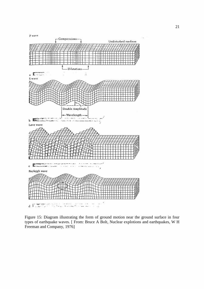
See figure 15.

The reflection and refraction in a boundary of two materials of one kind of incident body

waves may generate both kinds of body waves. The partitioning of the incident energy into

the four components, two in reflection and two in refraction, depends on the incident angle

and on the relative properties of the two media. That is why the earthquake ground motion is

very complex.

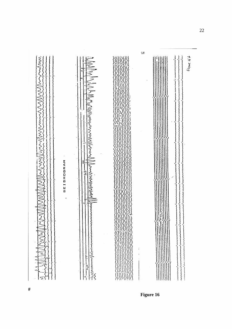
Because of the difference in velocity of these various waves, different waves arrive at

different times at the site. See figure 16. Therefore, knowing the velocity profile of the earth,

it is possible to estimate the distance of the source to the site. Seismologists use this

information from many sites to locate the epicentre and the focal depth of the earthquake.

Since there are four unknowns in the location of epicentres i.e. the latitude, the longitude,

the focal depth and the origin time of the earthquake, a minimum of 4 stations is required to

locate the source of the earthquake. International Seismological Centre (ISC) in Newbury,

Berkshire is equipped to collect the station information from all over the world and determine

the hypocentre with as much accuracy as possible by using least-square fitting technique.

NEIC (National Earthquake Information Centre- USGS) in the USA is another similar centre.

There are centres in every country which collects data from stations in that country and

determine epicentres. NEIC also determines magnitudes and moments of earthquakes. ISC

usually does not determine magnitudes and moments but reports those given by NEIC and

other stations.

21

Figure 15: Diagram illustrating the form of ground motion near the ground surface in four

types of earthquake waves. [ From: Bruce A Bolt, Nuclear explotions and earthquakes, W H

Freeman and Company, 1976]

22

#

Figure 16

23

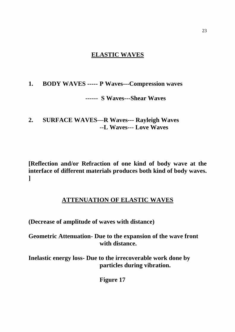
ELASTIC WAVES

1. BODY WAVES ----- P Waves---Compression waves

------ S Waves---Shear Waves

2. SURFACE WAVES—R Waves--- Rayleigh Waves

--L Waves--- Love Waves

[Reflection and/or Refraction of one kind of body wave at the

interface of different materials produces both kind of body waves.

]

ATTENUATION OF ELASTIC WAVES

(Decrease of amplitude of waves with distance)

Geometric Attenuation- Due to the expansion of the wave front

with distance.

Inelastic energy loss- Due to the irrecoverable work done by

particles during vibration.

Figure 17

24

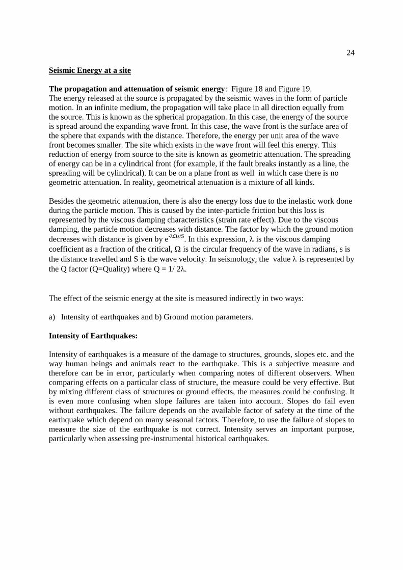
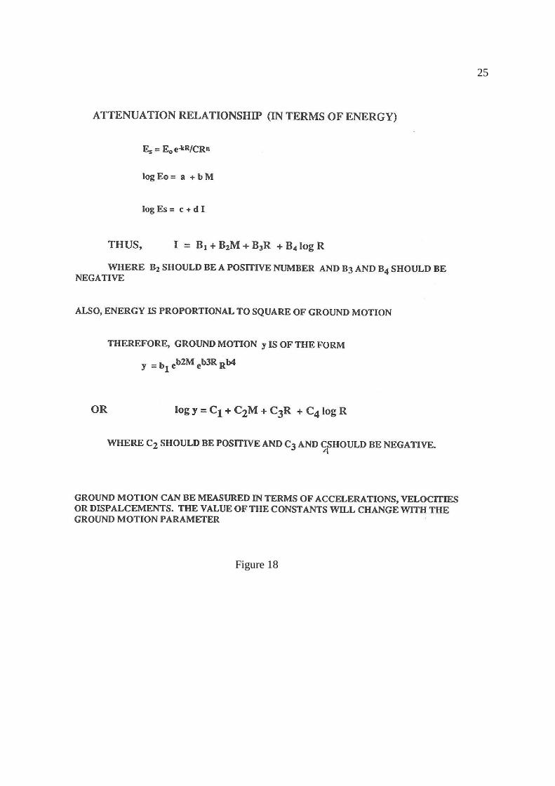
Seismic Energy at a site

The propagation and attenuation of seismic energy: Figure 18 and Figure 19.

The energy released at the source is propagated by the seismic waves in the form of particle

motion. In an infinite medium, the propagation will take place in all direction equally from

the source. This is known as the spherical propagation. In this case, the energy of the source

is spread around the expanding wave front. In this case, the wave front is the surface area of

the sphere that expands with the distance. Therefore, the energy per unit area of the wave

front becomes smaller. The site which exists in the wave front will feel this energy. This

reduction of energy from source to the site is known as geometric attenuation. The spreading

of energy can be in a cylindrical front (for example, if the fault breaks instantly as a line, the

spreading will be cylindrical). It can be on a plane front as well in which case there is no

geometric attenuation. In reality, geometrical attenuation is a mixture of all kinds.

Besides the geometric attenuation, there is also the energy loss due to the inelastic work done

during the particle motion. This is caused by the inter-particle friction but this loss is

represented by the viscous damping characteristics (strain rate effect). Due to the viscous

damping, the particle motion decreases with distance. The factor by which the ground motion

decreases with distance is given by e-s/S

. In this expression, is the viscous damping

coefficient as a fraction of the critical, is the circular frequency of the wave in radians, s is

the distance travelled and S is the wave velocity. In seismology, the value is represented by

the Q factor (Q=Quality) where Q = 1/ 2

The effect of the seismic energy at the site is measured indirectly in two ways:

a) Intensity of earthquakes and b) Ground motion parameters.

Intensity of Earthquakes:

Intensity of earthquakes is a measure of the damage to structures, grounds, slopes etc. and the

way human beings and animals react to the earthquake. This is a subjective measure and

therefore can be in error, particularly when comparing notes of different observers. When

comparing effects on a particular class of structure, the measure could be very effective. But

by mixing different class of structures or ground effects, the measures could be confusing. It

is even more confusing when slope failures are taken into account. Slopes do fail even

without earthquakes. The failure depends on the available factor of safety at the time of the

earthquake which depend on many seasonal factors. Therefore, to use the failure of slopes to

measure the size of the earthquake is not correct. Intensity serves an important purpose,

particularly when assessing pre-instrumental historical earthquakes.

25

Figure 18

26

Figure 19

There are several intensity scales that are presently in use. The most common is perhaps the

Modified Mercalli Scale, developed originally by Mercalli in 1902 and later modified by

Wood (1932). The most common scale used in Europe is MSK scale (Medvedev, Sponheur,

Karnik). The scales are more or less similar.

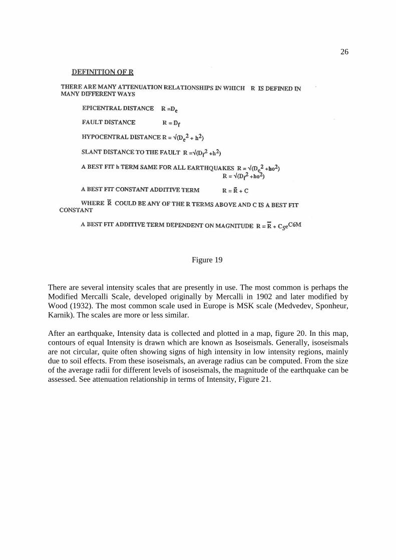
After an earthquake, Intensity data is collected and plotted in a map, figure 20. In this map,

contours of equal Intensity is drawn which are known as Isoseismals. Generally, isoseismals

are not circular, quite often showing signs of high intensity in low intensity regions, mainly

due to soil effects. From these isoseismals, an average radius can be computed. From the size

of the average radii for different levels of isoseismals, the magnitude of the earthquake can be

assessed. See attenuation relationship in terms of Intensity, Figure 21.

27

The Modified Mercalli Scale:

I Not felt except by a very few under especially favourable circumstances.

II Felt only by a few persons at rest, especially on upper floors of buildings. Delicately

suspended objects may swing.

III Felt quite noticeably indoors, especially on upper floors of buildings but many people

do not recognise it as an earthquake. Standing motor cars may rock slightly. Vibration

like passing trucks. Duration estimated.

IV During the day, felt indoors by many and outdoors by few. At night some awakened.

Dishes, windows, doors disturbed; walls make creaking sound. Sensation like heavy

truck striking building. Standing motor cars rocked noticeably.

V Felt by nearly everyone; many awakened. Some dishes, windows etc. broken; a few

instances of cracked plaster; unstable objects overturned. Disturbances of trees, poles

and other tall objects sometimes noticed. Pendulum clocks may stop

VI Felt by all; many frightened and run outdoors. Some heavy furniture moved; a few

instances of fallen plasters or damaged chimneys. Damage slight.

VII Everybody run outdoors. Damage negligible in buildings of good design and

construction; slight to moderate in well-built ordinary structures; considerable in

poorly built or badly designed structures; some chimneys broken. Noticed by persons

driving motor cars.

VIII Damage slight in specially designed structures; considerable in ordinary substantial

buildings with partial collapse; great in poorly built structures. Panel walls thrown out

of frame structures. Fall of chimneys, factory stacks, columns, monuments, walls.

Heavy furniture overturned. Sand and mud ejected in small amounts. Changes in well

water. Disturbs persons driving motor cars.

IX Damage considerable in especially designed structures; well designed frame

structures thrown out of plumb; great in substantial buildings with partial collapse.

Buildings shifted off foundations. Ground cracked conspicuously. Underground pipes

broken.

X Some well-built wooden structures destroyed; most masonry and frame structures

destroyed with foundations; ground badly cracked. Rails bent. Landslides

considerable from river banks and steep slopes. Shifted sand and mud. Water splashed

over banks.

XI Few, if any, (masonry) structures remain standing. Bridges destroyed. Broad fissures

in ground. Underground pipelines completely out of service. Earth slumps and land

slips on soft ground. Rails bent greatly.

XII Damage total. Waves seen on ground surfaces. Lines of sight and level distorted.

Objects thrown upward into the air.

28

Figure 20

Figure 21

29

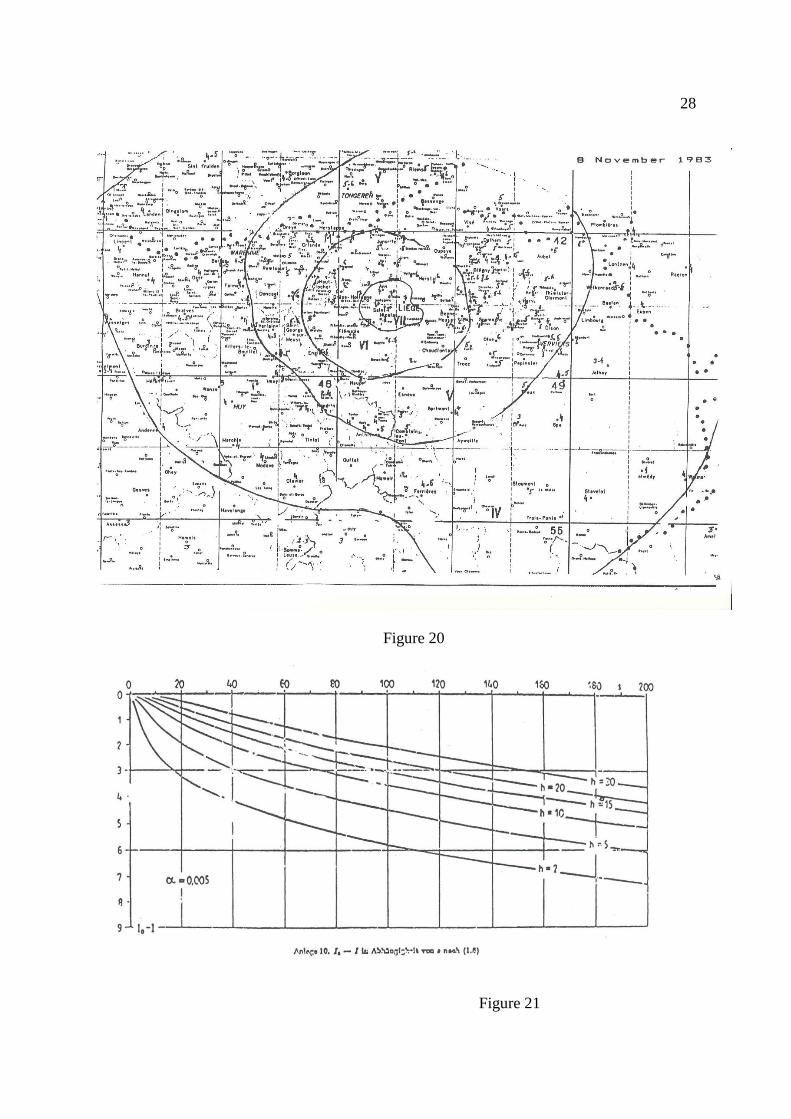
Ground Motion:

The effect of the energy at the site can also be measured by the ground motion parameters.

The ground motion is measured in terms of accelerations in the near field of earthquakes by

using the "Strong motion" instruments. The engineers use these. Seismologists use ground

displacements to determine epicentres and other source parameters. These are measured by

"Seismographs". Both strong motion instruments and seismographs produce time-history

records.

Theoretically, acceleration records can be integrated to obtain ground velocity and

displacements. However, there are problems associated with the integration process coming

from the "noise" in the records. Therefore, often the displacements obtained from integration

process is not reliable. (We do however use them after filtering out the noise, but filtering

process is not perfect.) Similarly, the displacement record obtained from seismographs can be

differentiated numerically to obtain velocity and accelerations. However, the numerical

differentiation process is always inaccurate when spikes are involved in the records. See

figure 22.

Figure 22

Now-a-days, banks of strong motion records exist (For example,ISESD, the strong motion

Data Bank originally stored at Imperial College) where, records from all over the world are

collected and processed. Because of their engineering importance, some owners of records

tend not to give the records away.

30

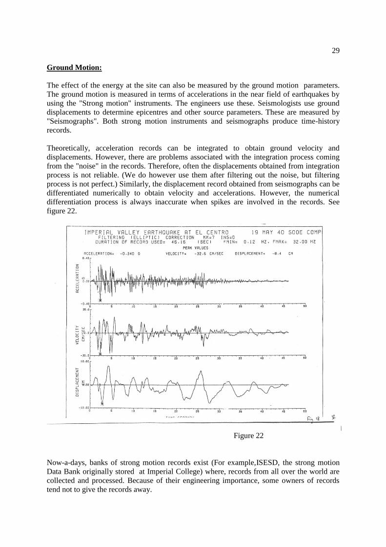
Attenuation of Strong motion Data:

Using the bank of data, attenuation relationships are derived for different ground motion

parameters by various authors. These relationships differ because of the choice of data from

the bank and the choice of the type of relationship. There are global relationships and there

are relationships derived from data from single countries. There are also relationships derived

from data of similar tectonic environments or of similar site geology. There can be many such

classifications. Because of the complex nature of the strong motion records, the relationships

appear to be crude with large standard deviations. Many attempts are going on to obtain

better relationships but not with much success. See figure 23.

Figure 23

31

The two most common relationships that are in use are

1. Ambraseys N. and Bommer J.(1991):

log a(g) = -1.09 +0.238 Ms -log r -.0005r +0.28p ; where r=(De2+ 6

2)

p=0 for mean value

p=1 for mean + 1sd

De = Shortest distance to the fault

rupture.

2. Joyner W.& Boore D. (1981):

log a(g) = -1.02 +0.249 M - log r -.00255r +0.26p ; where r=(De2+ 7.3

2)

Other definitions are same.

Sarma & Srbulov (1998) defined attenuation relationships for other ground motion

parameters.

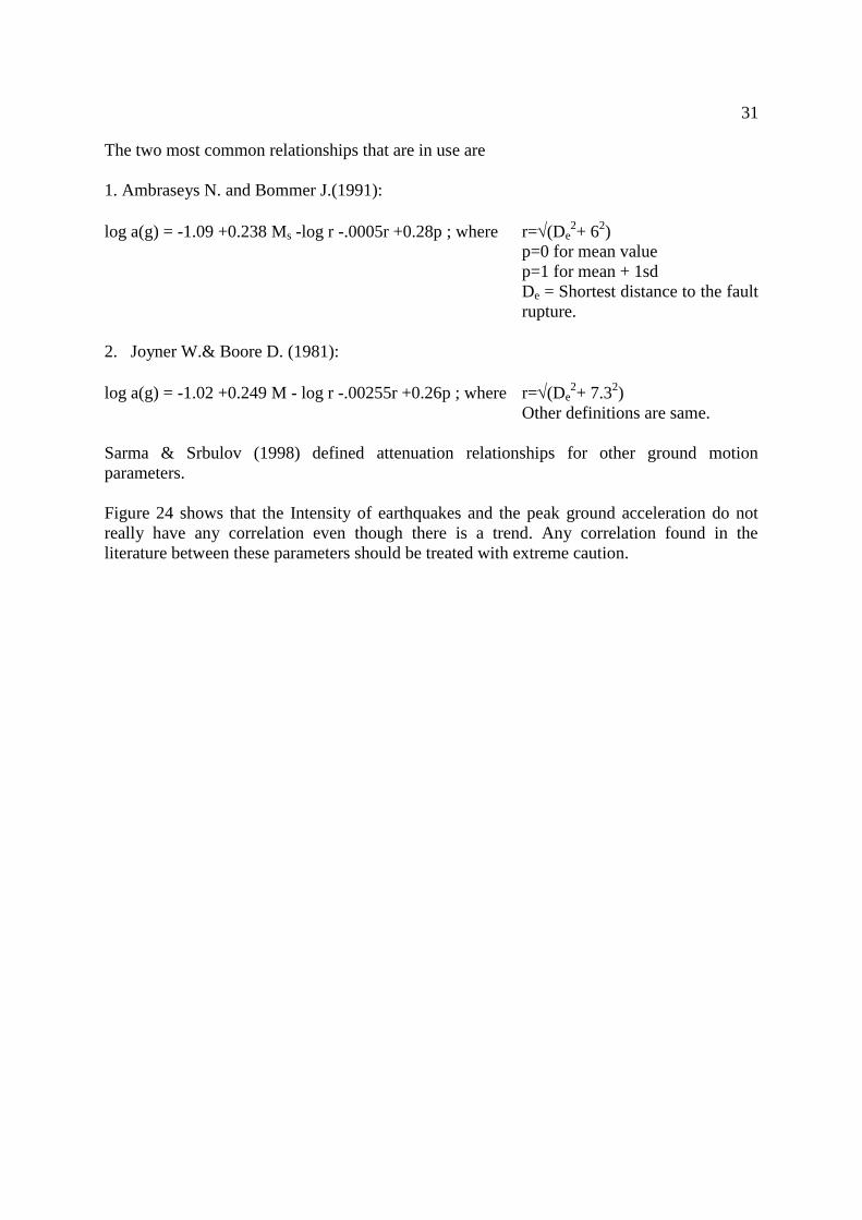
Figure 24 shows that the Intensity of earthquakes and the peak ground acceleration do not

really have any correlation even though there is a trend. Any correlation found in the

literature between these parameters should be treated with extreme caution.

32

Figure 24

33

References: [This is a reading list and not all are referenced in the text]

Ambraseys N., Free M. (1997) "Surface-wave magnitude calibration for European region

earthquakes", Journ. Earthq. Eng., 1, 1-22.

Ambraseys N., Melville C. (1982) A history of Persian earthquakes, Cambridge Univ. Press

Ambraseys N., Melville C. (1998) A catalogue of earthquakes in Iran up to 1996, Imperial

College Press (forthcoming)

Anderson J.G., Luco J.E. (1983) "Consequence of slip rate constrains on earthquake

occurrence relations", Bull. Seism. Soc. Am., 73, 471-496

Bath M. (1960) "Seismicity of Europe",Monogr. Union Geodes. & Geoph., no.1,pp.1-24,

Paris

Bath M.(1966): Earthquake energy and magnitude. Physics and Chemistry of the Earth. 7,

115-165.

Bath M. (1978) "A note on recurrence relations for earthquakes", Tectonophysics, vol.51,

pp.T23-T30

Bath, M. (1979) "A note on frequency and energy relations for earthquakes", Tectonophysics,

vol.56, pp.T27 - T33

Bath, M. (1981) "Earthquake magnitude - recent research and current trends", Earth-Sci.

Reviews, vol.17, pp.315-398

Cornell C.A. (1968) "Engineering seismic risk analysis" Bull. Seism. Soc. Am., vol.58,

pp.1583-1606

Ekstrom G., Dziewonski A.M. (1988) "Evidence of bias in the estimation of earthquake size"

Nature, vol.332, pp.319-23

Gutenberg B., Richter C. (1944) "Frequency of earthquakes in California", Bull. Seism. Soc.

Am., vol.34, p.186

Gutenberg B., Richter C. (1949) "Seismicity of the Earth and associated phenomena",

Princeton U.P. (reprinted and improved in 1954 & 1965)

Gutenberg B. & Richter C.(1956): Magnitude and energy of earthquakes. Annali di

Geofisica, 9, 1-15

Hanks T., Kanamori H. (1979) "A moment magnitude scale", J. Geophys. Res., vol. 84, B2,

pp.2348-2340

Ishimoto M., Iida K. (1939) "Observations sur les seismes enregistres par le

microseismographe construit dernierement", Bull. Earthq. Res. Inst., Pt.1, vol.17, pp.443-78

34

Kanamori H & Anderson D.(1975): Theoretical basis of some empirical relations in

seismology, Bull Seis. Soc. of America , 65, 5, 1073-1095.

Matuzawa T. (1941) "Uber die empirische Formel von Ishimoto und Iida", Bull. Earthq. Res.

Inst., Pt. 2, vol.19, pp.411-15

Molnar P. (1979) "Earthquake recurrence intervals and plate tectonics", Bull. Seism. Soc.

Am., vol.69, pp.115-33

Papastamatiou D., Sarma S.K. (1988) "Physical constraints in engineering seismic hazard

analysis", J. Earthq. Eng. Struct. Dynam., vol.16, pp.967-987

Richter C. (1958) Elementary Seismology, p. 359, Freeman

Attenuation Relationships:

Ambraseys N, Douglas J, Sarma S, Smit P. (2005a): Equations for the estimation of strong

ground motion from shallow crustal earthquakes using data from Europe and the Middle

East: Horizontal peak ground acceleration and spectral acceleration. Bull. Earthquake Engg,

3, 1-53.

Ambraseys N, Douglas J, Sarma S, Smit P. (2005b): Equations for the estimation of strong

ground motion from shallow crustal earthquakes using data from Europe and the Middle

East: Vertical peak ground acceleration and spectral acceleration. Bull. Earthquake Engg, 3,

55-79.

Ambraseys N. and Bommer J.(1991): The attenuation of ground accelerations in Europe.

Earthquake Engg. & Str. Dyn. 20, 1179-1202.

Ambraseys N. & Bommer J. (1995): Attenuation relations for use in Europe: An overview.

Proc. 5th

SECED Conf. on European Seismic Design Practice. ed. A.Elnashai, Chester, UK.

Arias A. (1970): A measure of earthquake Intensity. in Seismic Design for Nuclear Power

Plants. MIT Press, Cambridge, Massachusetts, 438-483.

Bolt B.A. (1973): Duration of strong motion. Proc. 5th

World Conf. Earthq. Engg. Rome,

Italy, 1, 1304-1315.

Bolt B.A. (1978): Earthquakes - a primer. W.H.Freeman.

Douglas J (2008): Ground motion estimation equations. Research Report BRGM/RP-56187-

FR

Joyner W.& Boore D. (1981):Peak horizontal acceleration and velocity from strong motion

records. Bull. Seis. Soc. Am., 71, 2011-2038.

35

Sarma & Srbulov (1998): A uniform estimation of some basic ground motion parameters.

Jour. Earthquake Engg., 2, 2, 267-287.

Bibliography on Engineering Seismology

The comments on the books are that of Dr. Julian Bommer, a colleague at Imperial College.

Aki K. & Richards P. (1980): Quantitative Seismology: theory & methods. 2 Volumes, W.H.

Freeman. A comprehensive and thorough text book for pure seismology, but mathematically

extremely demanding.

Algermissen S.T. (1983): An introduction to the seismicity of the United States. EERI

Monograph, Earthquake Engineering Research Institute. A clear and concise illustration of

seismicity and seismic hazard evaluation applied to the US.

Bath M.(1973): Introduction to seismology. Birkhauser Verlag. A very clearly written

introduction to the fundamental elements of seismology.

Bolt B. A. (1976): Nuclear explosions and earthquakes: the parted veil. W.H. Freeman. The

first part of this text provides a very clear explanation of many important seismological

concepts, and the reminder is a fascinating account of the application of seismology to the

enforcement of the atomic test ban treaties.

Bolt B.A. (1978) : Earthquakes - a primer. W.H. Freeman. This book is not written for

engineers but it is very readable and provides an excellent introduction to seismology and

earthquake engineering.

Bullen K.E. & Bolt B.A. (1985): An introduction to the theory of seismology. 4th

edition,

Cambridge Univ. Press. A very thorough text covering a very wide range of subjects.

Mathematically difficult in parts.

Condie K.C. (1989): Plate tectonics and crustal evolution. Pergamon Press. A clear and up-

to-date text on plate tectonics, although there are several others on this subject that could be

consulted as well.

Dowrick D.J. (1987): Earthquake resistant design for engineers and architects. 2nd

edition,

Wiley. The main emphasis of this book is earthquake resistant design, but the early chapters

provide a clear and concise introduction to the assessment of seismicity and seismic hazard.

36

Appendix SEISMICITY & HAZARD EVALUATION OF A SITE

In order to evaluate the seismic hazard of an engineering site we need the following

information.

a) Historical seismicity of the region;

b) Geology and tectonics of the region;

c) A mathematical (statistical) model for analysis;

d) Local soil conditions at the site.

In general, the hazard analysis concerns with the first three factors while the local soil

conditions are considered as a special case if necessary.

The study begins with the establishment of the region of interest around the site, which in

general could be large, say 5ox5o or even bigger. The idea is to establish regions within this area

which can be called homogeneous in the seismic sense, i.e. that the region belongs to the same

tectonic province, the earthquakes within the area has the same sort of mechanisms.

Historical seismicity of the region:

For the area in question, we then collect all the data about the earthquakes, i.e. the size

(magnitude, moment), location (epicentre, focal depth) that has happened in the past. The data

can be divided into two groups, instrumental data and pre-instrumental historical data.

The instrumental data can be obtained from the International Seismological Centre (ISC in

UK), the National earthquake Information Centre (NEIC in USA) and the National

Geophysical Data Centre(NGDC in USA). These agencies can supply data covering the period

from 1906 to the present. The accuracy associated with the instrumental data varies with time.

At the early stage, the errors associated could be large, particularly with epicentre determination

(±25km). There are instances of gross errors in locations. The reason being very few

instruments, unevenly located around the world and with low sensitivity. The location errors in

the present time could be ±5km. In the early period, smaller events were not located and

therefore incomplete.

The locations of pre-instrumental period earthquakes are obtained from historical studies,

extending the period as far back as possible. Obviously, the historical earthquakes will

concentrate on the large events. The magnitudes are determined from macro-seismic

information, such as felt radius or epicentral Intensity.

The magnitude determination for the instrumental period is non-homogeneous in the sense

that different formulae were used in different periods. It is often necessary to recalculate

magnitudes in a homogeneous way from the original data or look for published data. The error

associated with magnitudes could be of the order of ±0.25.

The focal depth determination is not accurate at all. In the early period, the focal depth was

generally given as 'Normal' or 33 km depth. In the catalogues, 33 km depth usually implies

37

unknown shallow focus earthquake. Even in the present day, errors associated with focal depth

determination could be large.

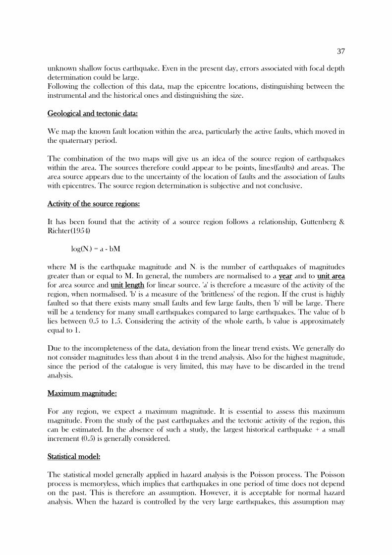
Following the collection of this data, map the epicentre locations, distinguishing between the

instrumental and the historical ones and distinguishing the size.

Geological and tectonic data:

We map the known fault location within the area, particularly the active faults, which moved in

the quaternary period.

The combination of the two maps will give us an idea of the source region of earthquakes

within the area. The sources therefore could appear to be points, lines(faults) and areas. The

area source appears due to the uncertainty of the location of faults and the association of faults

with epicentres. The source region determination is subjective and not conclusive.

Activity of the source regions:

It has been found that the activity of a source region follows a relationship, Guttenberg &

Richter(1954)

log(Nc) = a - bM

where M is the earthquake magnitude and Nc is the number of earthquakes of magnitudes

greater than or equal to M. In general, the numbers are normalised to a year and to unit area

for area source and unit length for linear source. 'a' is therefore a measure of the activity of the

region, when normalised. 'b' is a measure of the 'brittleness' of the region. If the crust is highly

faulted so that there exists many small faults and few large faults, then 'b' will be large. There

will be a tendency for many small earthquakes compared to large earthquakes. The value of b

lies between 0.5 to 1.5. Considering the activity of the whole earth, b value is approximately

equal to 1.

Due to the incompleteness of the data, deviation from the linear trend exists. We generally do

not consider magnitudes less than about 4 in the trend analysis. Also for the highest magnitude,

since the period of the catalogue is very limited, this may have to be discarded in the trend

analysis.

Maximum magnitude:

For any region, we expect a maximum magnitude. It is essential to assess this maximum

magnitude. From the study of the past earthquakes and the tectonic activity of the region, this

can be estimated. In the absence of such a study, the largest historical earthquake + a small

increment (0.5) is generally considered.

Statistical model:

The statistical model generally applied in hazard analysis is the Poisson process. The Poisson

process is memoryless, which implies that earthquakes in one period of time does not depend

on the past. This is therefore an assumption. However, it is acceptable for normal hazard

analysis. When the hazard is controlled by the very large earthquakes, this assumption may

38

lead to errors.

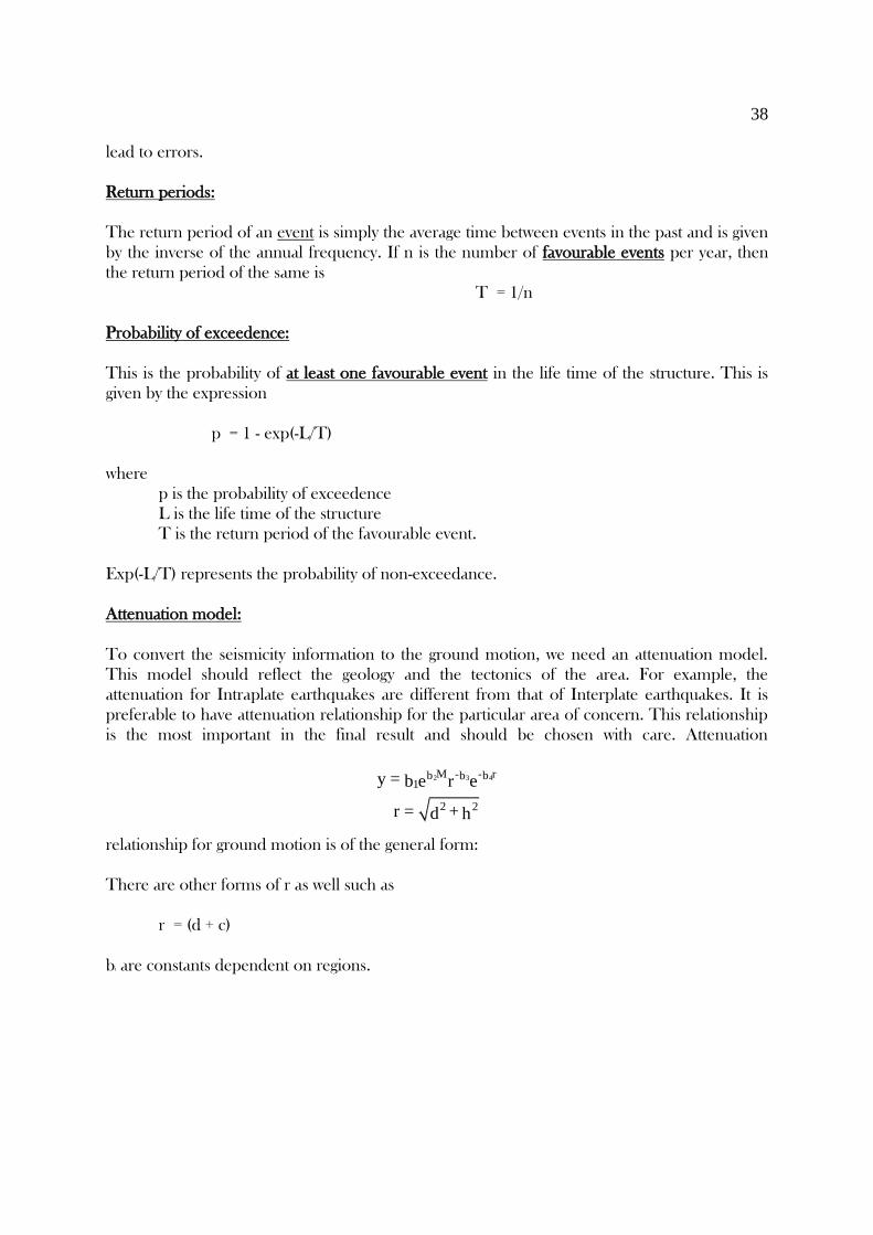
Return periods:

The return period of an event is simply the average time between events in the past and is given

by the inverse of the annual frequency. If n is the number of favourable events per year, then

the return period of the same is

T = 1/n

Probability of exceedence:

This is the probability of at least one favourable event in the life time of the structure. This is

given by the expression

p = 1 - exp(-L/T)

where

p is the probability of exceedence

L is the life time of the structure

T is the return period of the favourable event.

Exp(-L/T) represents the probability of non-exceedance.

Attenuation model:

To convert the seismicity information to the ground motion, we need an attenuation model.

This model should reflect the geology and the tectonics of the area. For example, the

attenuation for Intraplate earthquakes are different from that of Interplate earthquakes. It is

preferable to have attenuation relationship for the particular area of concern. This relationship

is the most important in the final result and should be chosen with care. Attenuation

relationship for ground motion is of the general form:

There are other forms of r as well such as

r = (d + c)

bi are constants dependent on regions.

2 43M - r-b bb1

2 2

y = b e er

r = +d h

39

Hazard Evaluation:

Point Source Model: This model is the basic “building block” for more elaborate source model

such as a fault line source or an area source. In this model, a point source with an expected

recurrence relationship (a,b parameters) is situated at a given distance (R) from the site and an

attenuation relationship exist for the region.

For the point source model, there are two approaches that can be adopted for the analysis.

A) Direct approach: Given the expected life (L) of a structure and the acceptable probability of

exceedance (p), we can determine the return period (T) of the event. Thus

p = 1- exp (-L/T)

The return period (T) is the inverse of the average number (n) of earthquakes per year.

T = 1/n

(n) is related to the magnitude of the earthquake through the recurrence relationship

log(n)= a-bM

(Note: If the computed magnitude is bigger than the maximum magnitude, then M is the

maximum magnitude)

From the magnitude of the event and the distance, we find the design ground motion.

2 43M - R-b bb1y = b e eR

(Note: In this relatonship, R is a distance parameter and not the distance directly).

Because of the presence of the maximum magnitude, this approach is applicable for a point

source only.

B) Indirect approach: This approach can be extended to more elaborate source models. This

is a reverse procedure from the direct approach.

We start with an assumed value of the ground motion y and determine its return period T

which is then related to p.

y => M => n => T

40

Plot y versus T and determine the design ground motion from the plot.

Many point sources model:

In this model, for any given value of the ground motion (y), the (n) values from all point

sources are added together. The return period is then given by:

T = 1/Σn