empirical exchange rate models of the nineties: are …mchinn/ccg-p_jimf.pdf2 meese and rogoﬀ...

Journal of International Money and Finance

24 (2005) 1150e1175

www.elsevier.com/locate/econbase

Empirical exchange rate models of thenineties: Are any fit to survive?

Yin-Wong Cheung a,*, Menzie D. Chinn b,Antonio Garcia Pascual c

a Department of Economics, E2, University of California, Santa Cruz, CA 95064, USAb LaFollette School of Public Affairs and Department of Economics, University of Wisconsin

and NBER, 1180 Observatory Drive, Madison, WI 53706, USAc International Monetary Fund, 700 19th Street NW, Washington, DC 20431, USA

Abstract

We re-assess exchange rate prediction using a wider set of models that have been proposedin the last decade: interest rate parity, productivity based models, and a composite specifica-

tion. The performance of these models is compared against two reference specifications e pur-chasing power parity and the sticky-price monetary model. The models are estimated infirst-difference and error correction specifications, and model performance evaluated at fore-

cast horizons of 1, 4 and 20 quarters, using the mean squared error, direction of changemetrics, and the ‘‘consistency’’ test of Cheung and Chinn [1998. Integration, cointegration,and the forecast consistency of structural exchange rate models. Journal of International

Money and Finance 17, 813e830]. Overall, model/specification/currency combinations thatwork well in one period do not necessarily work well in another period.� 2005 Elsevier Ltd. All rights reserved.

JEL classification: F31; F47

Keywords: Exchange rates; Monetary model; Productivity; Interest rate parity; Purchasing power parity;

Forecasting performance

* Corresponding author. Tel.: C1 831 459 4247; fax: C1 831 459 5900.

E-mail address: [email protected] (Y.-W. Cheung).

0261-5606/$ - see front matter � 2005 Elsevier Ltd. All rights reserved.

doi:10.1016/j.jimonfin.2005.08.002

mailto:[email protected]

http://www.elsevier.com/locate/econbase

1151Y.-W. Cheung et al. / Journal of International Money and Finance 24 (2005) 1150e1175

1. Introduction

The recent movements in the dollar and the euro have appeared seemingly inex-plicable in the context of standard models. While the dollar may not have been ‘‘daz-zling’’ e as it was described in the mid-1980s e it has been characterized as overly‘‘darling.’’1 And the euro’s ability to repeatedly confound predictions needs littlere-emphasizing.

It is against this backdrop that several new models have been forwarded in thepast decade. Some explanations are motivated by findings in the empirical and the-oretical literature, such as the correlation between net foreign asset positions and realexchange rates and those based on productivity differences. None of these models,however, have been subjected to rigorous examination of the sort that Meese andRogoff conducted in their seminal work, the original title of which we have appro-priated and amended for this study.2

We believe that a systematic examination of these newer empirical models is longoverdue, for a number of reasons. First, while these models have become prominentin policy and financial circles, they have not been subjected to the sort systematicout-of-sample testing conducted in academic studies. For instance, productivitydid not make an appearance in earlier comparative studies, but has been tappedas an important determinant of the euroedollar exchange rate (Owen, 2001; Rosen-berg, 2000).3

Second, most of the recent academic treatments’ exchange rate forecasting perfor-mance relies upon a single model e such as the monetary model e or some otherlimited set of models of 1970s’ vintage, such as purchasing power parity or real in-terest differential model.

Third, the same criteria are often used, neglecting alternative dimensions of modelforecast performance. That is, the first and second moment metrics such as mean er-ror and mean squared error are considered, while other aspects that might be ofgreater importance are often neglected. We have in mind the direction of change eperhaps more important from a market timing perspective e and other indicators offorecast attributes.

In this study, we extend the forecast comparison of exchange rate models in sev-eral dimensions.

� Five models are compared against the random walk. Purchasing power parity isincluded because of its importance in the international finance literature and the

1 Frankel (1985) and The Economist (2001), respectively.2 Meese and Rogoff (1983) was based upon work in ‘‘Empirical exchange rate models of the seventies:

are any fit to survive?’’ International Finance Discussion PaperNo. 184 (Board of Governors of the Federal

Reserve System, 1981).3 Similarly, behavioral equilibrium exchange rate (BEER) models e essentially combinations of real in-

terest differential, nontraded goods and portfolio balance models e have been used in estimating the

‘‘equilibrium’’ values of the euro. See Bank of America (Yilmaz, 2003), Bundesbank (Clostermann and

Schnatz, 2000), ECB (Schnatz et al., 2004), and IMF (Alberola et al., 1999). A corresponding study for

the dollar is Yilmaz and Jen (2001).

1152 Y.-W. Cheung et al. / Journal of International Money and Finance 24 (2005) 1150e1175

fact that the parity condition is commonly used to gauge the degree of exchangerate misalignment. The sticky-price monetary model of Dornbusch and Frankelis the only structural model that has been the subject of previous systematic anal-yses. The other models include one incorporating productivity differentials, aninterest rate parity specification, and a composite specification incorporatinga number of channels identified in differing theoretical models.

� The behavior of US dollar-based exchange rates of the Canadian dollar, Britishpound, Deutsche mark and Japanese yen are examined. To insure that our con-clusions are not driven by dollar specific results, we also examine (but do not re-port) the results for the corresponding yen-based rates.

� The models are estimated in two ways: in first-difference and error correctionspecifications.

� Forecasting performance is evaluated at several horizons (1-, 4- and 20-quarterhorizons) and in two sample periods (post-Louvre Accord and post-1982).

� We augment the conventional metrics with a direction of change statistic and the‘‘consistency’’ criterion of Cheung and Chinn (1998).

Before proceeding further, it may prove worthwhile to emphasize why we focuson out-of-sample prediction as our basis of judging the relative merits of the models.It is not that we believe that we can necessarily out-forecast the market in real time.Indeed, our forecasting exercises are in the nature of ex post simulations, where inmany instances contemporaneous values of the right-hand-side variables are usedto predict future exchange rates. Rather, we construe the exercise as a means of pro-tecting against data mining that might occur when relying solely on in-sampleinference.4

The exchange rate models considered in the exercise are summarized in Section 2.Section 3 discusses the data, the estimation methods, and the criteria used to com-pare forecasting performance. The forecasting results are reported in Section 4. Sec-tion 5 concludes.

2. Theoretical models

The universe of empirical models that has been examined over the floating rateperiod is enormous. Consequently any evaluation of these models must necessarilybe selective. Our criteria require that the models are (1) prominent in the economicand policy literature, (2) readily implementable and replicable, and (3) not previouslyevaluated in a systematic fashion. We use the random walk model as our benchmarknaive model, in line with previous work, but we also select the purchasing power par-ity and the basic Dornbusch (1976) and Frankel (1979) model as two comparatorspecifications, as they still provide the fundamental intuition on how flexible

4 There is an enormous literature on data mining. See Inoue and Kilian (2004) for some recent thoughts

on the usefulness of out-of-sample versus in-sample tests.


exchange rates behave. The purchasing power parity condition examined in thisstudy is given by

stZb0Cpt; ð1Þ

where s is the log exchange rate, p is the log price level (CPI), and ‘‘ ˆ ’’ denotes theintercountry difference. Strictly speaking, Eq. (1) is the relative purchasing powerparity condition. The relative version is examined because price indices ratherthan the actual price levels are considered.

The sticky-price monetary model can be expressed as follows:

stZb0Cb1mtCb2ytCb3 itCb4ptCut; ð2Þ

wherem is log money, y is log real GDP, i and p are the interest and inflation rates, re-spectively, and ut is an error term. The characteristics of this model are well known, sowewill not devote time to discussing the theory behind the equation.Wenote, however,that the list of variables included in Eq. (2) encompasses those employed in the flexibleprice version of the monetary model, as well as the micro-based general equilibriummodels of Stockman (1980) and Lucas (1982). In addition, two observations are in or-der. First, the sticky-price model can be interpreted as an extension of Eq. (1) such thatthe price variables are replaced by macro variables that capture money demand andovershooting effects. Second, we do not impose coefficient restrictions in Eq. (2) be-cause theory gives us little guidance regarding the exact values of all the parameters.

Next, we assess models that are in the BalassaeSamuelson vein, in that they ac-cord a central role to productivity differentials to explaining movements in real, andhence also nominal, exchange rates. Real versions of the model can be traced to De-Gregorio and Wolf (1994), while nominal versions include Clements and Frenkel(1980) and Chinn (1997). Such models drop the purchasing power parity assumptionfor broad price indices, and allow the real exchange rate to depend upon the relativeprice of nontradables, itself a function of productivity (z) differentials. A generic pro-ductivity differential exchange rate equation is

stZb0Cb1mtCb2ytCb3 itCb5ztCut: ð3Þ

Although Eqs. (2) and (3) bear a superficial resemblance, the two expressions em-body quite different economic and statistical implications. The central difference isthat Eq. (2) assumes PPP holds in the long run, while the productivity based modelmakes no such presumption. In fact the nominal exchange rate can drift infinitely faraway from PPP, although the path is determined in this model by productivitydifferentials.

The fourth model is a composite model that incorporates a number of familiarrelationships. A typical specification is:

stZb0CptCb5utCb6rtCb7gdebttCb8tottCb9nfatCut; ð4Þ

where u is the relative price of nontradables, r the real interest rate, gdebt the gov-ernment debt to GDP ratio, tot the log terms of trade, and nfa is the net foreign


asset. Note that we impose a unitary coefficient on the intercountry log price level p,so that Eq. (4) could be re-expressed as determining the real exchange rate.

Although this particular specification closely resembles the behavioral equilibriumexchange rate (BEER) model of Clark and MacDonald (1999), it also shares attrib-utes with the NATREX model of Stein (1999) and the real equilibrium exchange ratemodel of Edwards (1989), as well as a number of other approaches. Consequently,we will henceforth refer to this specification as the ‘‘composite’’ model. Again, rela-tive to Eq. (1), the composite model incorporates the BalassaeSamuelson effect (viau), the overshooting effect (r), and the portfolio balance effect (gdebt, nfa).5

Models based upon this framework have been the predominant approach to de-termining the rate at which currencies will gravitate to over some intermediate hori-zon, especially in the context of policy issues. For instance, the behavioralequilibrium exchange rate approach is the model that is most often used to determinethe long-term value of the euro.6

The final specification assessed is not a model per se; rather it is an arbitrage re-lationship e uncovered interest rate parity:

stCkZstCii;k ð5Þ

where it,k is the interest rate of maturity k. Similar to the relative purchasing powerparity (1), this relation need not be estimated in order to generate predictions.

The interest rate parity is included in the forecast comparison exercise mainly be-cause it has recently gathered empirical support at long horizons (Alexius, 2001;Chinn and Meredith, 2004), in contrast to the disappointing results at the shorter ho-rizons. MacDonald and Nagayasu (2000) have also demonstrated that long-run in-terest rates appear to predict exchange rate levels. On the basis of these findings, weanticipate that this specification will perform better at the longer horizons than atshorter horizons.7

3. Data, estimation and forecasting comparison

3.1. Data

The analysis uses quarterly data for the United States, Canada, UK, Japan, Ger-many, and Switzerland over the 1973q2 to 2000q4 period. The exchange rate, money,price and income variables are drawn primarily from the IMF’s International

5 On this latter channel, Cavallo and Ghironi (2002) provide a role for net foreign assets in the determi-

nation of exchange rates in the sticky-price optimizing framework of Obstfeld and Rogoff (1995).6 We do not examine a closely related approach, the internaleexternal balance approach of the IMF (see

Faruqee et al., 1999). The IMF approach requires extensive judgments regarding the trend level of output,

and the impact of demographic variables upon various macroeconomic aggregates. We did not believe it

would be possible to subject this methodology to the same out-of-sample forecasting exercise applied to

the others.7 Despite this finding, there is little evidence that long-term interest rate differentials e or equivalently

long-dated forward rates e have been used for forecasting at the horizons we are investigating. One ex-

ception from the non-academic literature is Rosenberg (2001).


Financial Statistics. The productivity data were obtained from the Bank for Interna-tional Settlements, while the interest rates used to conduct the interest rate parityforecasts are essentially the same as those used in Chinn and Meredith (2004). Seethe Appendix 1 for a more detailed description.

Two out-of-sample periods are used to assess model performance: 1987q2e2000q4 and 1983q1e2000q4. The former period conforms to the post-Louvre Ac-cord period, while the latter spans the period after the end of monetary targetingin the US. The shorter out-of-sample period (1987e2000) spans a period of relativedollar stability (and appreciation in the case of the mark). The longer out-of-sampleperiod subjects the models to a more rigorous test, in that the prediction takes placeover a large dollar appreciation and subsequent depreciation (against the mark) anda large dollar depreciation (from 250 to 150 yen per dollar). In other words, this lon-ger span encompasses more than one ‘‘dollar cycle.’’ The use of this long out-of-sam-ple forecasting period has the added advantage that it ensures that there are manyforecast observations to conduct inference upon.

3.2. Estimation and forecasting

We adopt the convention in the empirical exchange rate modeling literature of im-plementing ‘‘rolling regressions’’ established by Meese and Rogoff. That is, estimatesare applied over a given data sample, out-of-sample forecasts produced, then thesample is moved up, or ‘‘rolled’’ forward one observation before the procedure is re-peated. This process continues until all the out-of-sample observations are ex-hausted. While the rolling regressions do not incorporate possible efficiency gainsas the sample moves forward through time, the procedure has the potential benefitof alleviating parameter instability effects over time e which is a commonly con-ceived phenomenon in exchange rate modeling.

Two specifications of these theoretical models were estimated: (1) an error correc-tion specification, and (2) a first-difference specification. These two specifications en-tail different implications for interactions between exchange rates and theirdeterminants. It is well known that both the exchange rate and its economic deter-minants are I(1). The error correction specification explicitly allows for the long-run interaction effect of these variables (as captured by the error correction term)in generating forecast. On the other hand, the first differences model emphasizesthe effects of changes in the macro variables on exchange rates. If the variablesare cointegrated, then the former specification is more efficient than the latter oneand is expected to forecast better in long horizons. If the variables are not cointe-grated, the error correction specification can lead to spurious results. Because it isnot easy to determine unambiguously whether these variables are cointegrated ornot, we consider both specifications.

Since implementation of the error correction specification is relatively involved,we will address the first-difference specification to begin with. Consider the generalexpression for the relationship between the exchange rate and fundamentals:

stZXtGC3t; ð6Þ


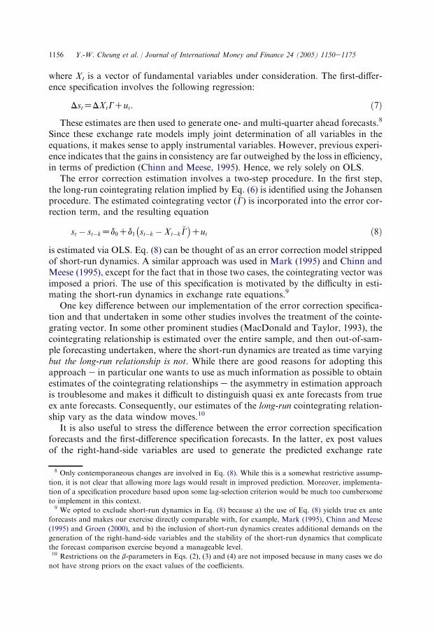
where Xt is a vector of fundamental variables under consideration. The first-differ-ence specification involves the following regression:

DstZDXtGCut: ð7Þ

These estimates are then used to generate one- and multi-quarter ahead forecasts.8

Since these exchange rate models imply joint determination of all variables in theequations, it makes sense to apply instrumental variables. However, previous experi-ence indicates that the gains in consistency are far outweighed by the loss in efficiency,in terms of prediction (Chinn and Meese, 1995). Hence, we rely solely on OLS.

The error correction estimation involves a two-step procedure. In the first step,the long-run cointegrating relation implied by Eq. (6) is identified using the Johansenprocedure. The estimated cointegrating vector (~G) is incorporated into the error cor-rection term, and the resulting equation

st � st�kZd0Cd1�st�k �Xt�k

~G�Cut ð8Þ

is estimated via OLS. Eq. (8) can be thought of as an error correction model strippedof short-run dynamics. A similar approach was used in Mark (1995) and Chinn andMeese (1995), except for the fact that in those two cases, the cointegrating vector wasimposed a priori. The use of this specification is motivated by the difficulty in esti-mating the short-run dynamics in exchange rate equations.9

One key difference between our implementation of the error correction specifica-tion and that undertaken in some other studies involves the treatment of the cointe-grating vector. In some other prominent studies (MacDonald and Taylor, 1993), thecointegrating relationship is estimated over the entire sample, and then out-of-sam-ple forecasting undertaken, where the short-run dynamics are treated as time varyingbut the long-run relationship is not. While there are good reasons for adopting thisapproach e in particular one wants to use as much information as possible to obtainestimates of the cointegrating relationships e the asymmetry in estimation approachis troublesome and makes it difficult to distinguish quasi ex ante forecasts from trueex ante forecasts. Consequently, our estimates of the long-run cointegrating relation-ship vary as the data window moves.10

It is also useful to stress the difference between the error correction specificationforecasts and the first-difference specification forecasts. In the latter, ex post valuesof the right-hand-side variables are used to generate the predicted exchange rate

8 Only contemporaneous changes are involved in Eq. (8). While this is a somewhat restrictive assump-

tion, it is not clear that allowing more lags would result in improved prediction. Moreover, implementa-

tion of a specification procedure based upon some lag-selection criterion would be much too cumbersome

to implement in this context.9 We opted to exclude short-run dynamics in Eq. (8) because a) the use of Eq. (8) yields true ex ante

forecasts and makes our exercise directly comparable with, for example, Mark (1995), Chinn and Meese

(1995) and Groen (2000), and b) the inclusion of short-run dynamics creates additional demands on the

generation of the right-hand-side variables and the stability of the short-run dynamics that complicate

the forecast comparison exercise beyond a manageable level.10 Restrictions on the b-parameters in Eqs. (2), (3) and (4) are not imposed because in many cases we do

not have strong priors on the exact values of the coefficients.


change. In the former, contemporaneous values of the right-hand-side variables arenot necessary, and the error correction predictions are true ex ante forecasts. Hence,we are affording the first-difference specifications a tremendous informational advan-tage in forecasting.

3.3. Forecast comparison

To evaluate the forecasting accuracy of the different structural models, the ratiobetween the mean squared error (MSE) of the structural models and a driftless ran-dom walk is used. A value smaller (larger) than one indicates a better performance ofthe structural model (random walk). Inferences are based on a formal test for thenull hypothesis of no difference in the accuracy (i.e. in the MSE) of the two compet-ing forecasts e structural model versus driftless random walk. In particular, we usethe DieboldeMariano statistic (Diebold and Mariano, 1995) which is defined as theratio between the sample mean loss differential and an estimate of its standard error;this ratio is asymptotically distributed as a standard normal.11 The loss differential isdefined as the difference between the squared forecast error of the structural modelsand that of the random walk. A consistent estimate of the standard deviation can beconstructed from a weighted sum of the available sample autocovariances of the lossdifferential vector. Following Andrews (1991), a quadratic spectral kernel is em-ployed, together with a data-dependent bandwidth selection procedure.12

We also examine the predictive power of the various models along different di-mensions. One might be tempted to conclude that we are merely changing thewell-established ‘‘rules of the game’’ by doing so. However, there are very good rea-sons to use other evaluation criteria. First, there is the intuitively appealing rationalethat minimizing the mean squared error (or relatedly mean absolute error) may notbe important from an economic standpoint. A less pedestrian motivation is that thetypical mean squared error criterion may miss out on important aspects of predic-tions, especially at long horizons. Christoffersen and Diebold (1998) point out thatthe standard mean squared error criterion indicates no improvement of predictionsthat take into account cointegrating relationships vis a vis univariate predictions. Butsurely, any reasonable criteria would put some weight on the tendency for predic-tions from cointegrated systems to ‘‘hang together.’’

Hence, our first alternative evaluation metric for the relative forecast performanceof the structural models is the direction of change statistic, which is computed as thenumber of correct predictions of the direction of change over the total number ofpredictions. A value above (below) 50% indicates a better (worse) forecasting

11 In using the DieboldeMariano test, we are relying upon asymptotic results, which may or may not be

appropriate for our sample. However, generating finite sample critical values for the large number of cases

we deal with would be computationally infeasible. More importantly, the most likely outcome of such an

exercise would be to make detection of statistically significant outperformance even more rare, and leaving

our basic conclusion intact.12 We also experienced with the Bartlett kernel and the deterministic bandwidth selection method. The

results from these methods are qualitatively very similar. Appendix 2 contains a more detailed discussion

of the forecast comparison tests.


performance than a naive model that predicts the exchange rate has an equal chanceto go up or down. Again, Diebold and Mariano (1995) provide a test statistic for thenull of no forecasting performance of the structural model. The statistic follows a bi-nomial distribution, and its studentized version is asymptotically distributed as a stan-dard normal. Not only does the direction of change statistic constitute an alternativemetric, Leitch and Tanner (1991), for instance, argue that a direction of change cri-terion may be more relevant for profitability and economic concerns, and hencea more appropriate metric than others based on purely statistical motivations. Thecriterion is also related to tests for market timing ability (Cumby and Modest, 1987).

The third metric we used to evaluate forecast performance is the consistency cri-terion proposed in Cheung and Chinn (1998). This metric focuses on the time-seriesproperties of the forecast. The forecast of a given spot exchange rate is labeled asconsistent if (1) the two series have the same order of integration, (2) they are coin-tegrated, and (3) the cointegration vector satisfies the unitary elasticity of expecta-tions condition. Loosely speaking, a forecast is consistent if it moves in tandemwith the spot exchange rate in the long run. While the two previous criteria focuson the precision of the forecast, the consistency requirement is concerned with thelong-run relative variation between forecasts and actual realizations. One may arguethat the criterion is less demanding than the MSE and direction of change metrics. Aforecast that satisfies the consistency criterion can (1) have an MSE larger than thatof the random walk model, (2) have a direction of change statistic less than 1/2, or(3) generate forecast errors that are serially correlated. However, given the problemsrelated to modeling, estimation, and data quality, the consistency criterion can bea more flexible way to evaluate a forecast. Cheung and Chinn (1998) providea more detailed discussion on the consistency criterion and its implementation.

It is not obvious which one of the three evaluation criteria is better as they eachhave a different focus. The MSE is a standard evaluation criterion, the direction ofchange metric emphasizes the ability to predict directional changes, and the consis-tency test is concerned about the long-run interactions between forecasts and theirrealizations. Instead of arguing one criterion is better than the other, we considerthe use of these criteria as complementary and providing a multifaceted picture ofthe forecast performance of these structural models. Of course, depending on thepurpose of a specific exercise, one may favor one metric over the other.

4. Comparing the forecast performance

4.1. The MSE criterion

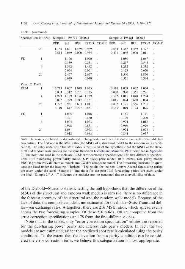
The comparison of forecasting performance based on MSE ratios is summarizedin Table 1. The table contains MSE ratios and the p-values from five dollar-based cur-rency pairs, five model specifications, the error correction and first-difference specifi-cations, three forecasting horizons, and two forecasting samples. Each cell in thetable has two entries. The first one is the MSE ratio (the MSEs of a structural modelto the random walk specification). The entry underneath the MSE ratio is the p-value


Table 1

The MSE ratios from the dollar-based exchange rates

Specification Horizon Sample 1: 1987q2e2000q4 Sample 2: 1983q1e2000q4

PPP S-P IRP PROD COMP PPP S-P IRP PROD COMP

Panel A: BP/$

ECM 1 4.165 1.047 1.008 0.995 1.085 5.678 1.050 1.046 1.042 1.049

0.003 0.409 0.883 0.897 0.208 0.031 0.310 0.318 0.303 0.448

4 1.750 1.127 1.092 1.017 1.099 1.612 1.142 1.123 1.085 1.127

0.199 0.503 0.620 0.802 0.253 0.224 0.171 0.310 0.237 0.225

20 0.782 1.809 1.342 1.095 1.340 0.632 1.457 0.841 1.545 2.179

0.536 0.014 0.240 0.411 0.168 0.156 0.071 0.518 0.092 0.057

FD 1 1.041 1.006 1.191 1.086 1.079 1.023

0.434 0.940 0.217 0.135 0.337 0.901

4 1.120 1.124 1.881 1.250 1.455 1.448

0.315 0.524 0.001 0.149 0.176 0.351

20 1.891 2.531 6.953 3.223 5.557 6.015

0.177 0.021 0.000 0.195 0.019 0.001

Panel B: CAN$/$

ECM 1 32.205 1.054 1.090 1.148 1.278 31.982 1.056 1.092 1.041 1.337

0.008 0.127 0.048 0.062 0.016 0.001 0.279 0.022 0.552 0.004

4 6.504 1.102 1.172 1.182 1.603 6.947 1.116 1.170 1.017 1.754

0.016 0.181 0.452 0.157 0.118 0.004 0.334 0.359 0.929 0.018

20 1.569 0.939 0.865 1.090 1.760 1.171 1.062 0.813 1.097 1.623

0.000 0.574 0.760 0.308 0.002 0.093 0.727 0.607 0.318 0.000

FD 1 1.100 1.115 0.614 1.101 1.171 0.666

0.179 0.138 0.109 0.257 0.047 0.151

4 1.137 1.160 0.899 1.196 1.269 1.143

0.461 0.341 0.798 0.347 0.192 0.704

20 0.515 0.504 1.924 1.892 2.004 2.289

0.193 0.182 0.006 0.182 0.143 0.204

Panel C: DM/$

ECM 1 6.357 1.059 1.030 1.041 0.995 11.173 1.105 1.029 0.997 0.911

0.006 0.464 0.295 0.574 0.955 0.005 0.416 0.364 0.961 0.206

4 2.301 1.080 1.136 1.080 1.116 2.675 1.104 1.063 0.949 0.898

0.016 0.444 0.069 0.282 0.642 0.007 0.599 0.485 0.626 0.558

20 0.649 1.047 0.596 1.131 2.137 0.411 1.771 0.895 1.260 0.633

0.363 0.637 0.167 0.141 0.216 0.248 0.212 0.656 0.039 0.202

FD 1 1.268 1.324 0.555 1.123 1.196 0.694

0.052 0.106 0.001 0.017 0.084 0.020

4 1.402 1.607 0.844 1.077 1.281 1.151

0.024 0.030 0.571 0.452 0.009 0.612

20 1.814 1.927 2.522 1.723 1.964 3.975

0.175 0.114 0.140 0.246 0.121 0.003

Panel D: SF/$

ECM 1 7.595 1.074 1.051 1.024 . 8.694 0.995 1.050 1.052 .

0.001 0.187 0.138 0.515 . 0.000 0.906 0.141 0.581 .

4 2.537 1.269 1.183 1.184 . 2.106 1.002 1.122 1.136 .

0.014 0.015 0.059 0.367 . 0.003 0.982 0.248 0.149 .

(continued on next page)


of the DieboldeMariano statistic testing the null hypothesis that the difference of theMSEs of the structural and random walk models is zero (i.e. there is no difference inthe forecast accuracy of the structural and the random walk model). Because of thelack of data, the composite model is not estimated for the dollareSwiss franc and dol-lareyen exchange rates. Altogether, there are 216 MSE ratios, which spread evenlyacross the two forecasting samples. Of these 216 ratios, 138 are computed from theerror correction specifications and 78 from the first-difference ones.

Note that in the tables, only ‘‘error correction specification’’ entries are reportedfor the purchasing power parity and interest rate parity models. In fact, the twomodels are not estimated; rather the predicted spot rate is calculated using the parityconditions. To the extent that the deviation from a parity condition can be consid-ered the error correction term, we believe this categorization is most appropriate.

Table 1 (continued)



20 1.185 1.621 1.489 0.969 . 0.634 1.367 1.489 1.377 .

0.514 0.069 0.000 0.934 . 0.431 0.046 0.000 0.011 .

FD 1 1.106 1.090 . 1.089 1.067 .

0.189 0.351 . 0.237 0.545 .

4 1.362 1.468 . 1.232 1.332 .

0.004 0.001 . 0.153 0.050 .

20 2.477 2.657 . 1.540 1.870 .

0.039 0.049 . 0.521 0.394 .

Panel E: Yen/$

ECM 1 15.713 1.067 1.049 1.073 . 10.510 1.008 1.032 1.064 .

0.003 0.312 0.251 0.125 . 0.000 0.920 0.361 0.281 .

4 4.973 1.189 1.174 1.239 . 2.582 1.015 1.048 1.234 .

0.022 0.279 0.247 0.151 . 0.015 0.874 0.658 0.004 .

20 1.797 0.951 0.603 1.011 . 0.832 1.175 0.566 1.235 .

0.149 0.647 0.227 0.851 . 0.585 0.049 0.174 0.076 .

FD 1 1.085 1.048 . 1.165 1.141 .

0.321 0.480 . 0.179 0.220 .

4 1.004 1.023 . 0.994 1.012 .

0.978 0.881 . 0.969 0.929 .

20 1.081 0.973 . 0.924 1.023 .

0.912 0.963 . 0.844 0.957 .

Note: The results are based on dollar-based exchange rates and their forecasts. Each cell in the table has

two entries. The first one is the MSE ratio (the MSEs of a structural model to the random walk specifi-

cation). The entry underneath the MSE ratio is the p-value of the hypothesis that the MSEs of the struc-

tural and random walk models are the same (based on Diebold and Mariano, 1995, described in Appendix

2). The notations used in the table are ECM: error correction specification; FD: first-difference specifica-

tion; PPP: purchasing power parity model; S-P: sticky-price model; IRP: interest rate parity model;

PROD: productivity differential model; and COMP: composite model. The forecasting horizons (in quar-

ters) are listed under the heading ‘‘Horizon.’’ The results for the post-Louvre Accord forecasting period

are given under the label ‘‘Sample 1’’ and those for the post-1983 forecasting period are given under

the label ‘‘Sample 2.’’ A ‘‘.’’ indicates the statistics are not generated due to unavailability of data.


Overall, the MSE results are not favorable to the structural models. Of the 216MSE ratios, 151 are not significant (at the 10% significance level) and 65 are signif-icant. That is, for the majority cases one cannot differentiate the forecasting perfor-mance between a structural model and a random walk model. For the 65 significantcases, there are 63 cases in which the random walk model is significantly better thanthe competing structural models and only two cases in which the opposite is true.The significant cases are quite evenly distributed across the two forecasting periods.As 10% is the size of the test and two cases constitute less than 10% of the total of216 cases, the empirical evidence can hardly be interpreted as supportive of the su-perior forecasting performance of the structural models.

Inspection of the MSE ratios does not reveal many consistent patterns in terms ofoutperformance. It appears that the productivity model does not do particularlybadly for the dollaremark rate at the 1- and 4-quarter horizons. The MSE ratiosof the purchasing power parity and interest rate parity models are less than unity(even though not significant) only at the 20-quarter horizon e a finding consistentwith the perception that these parity conditions work better at long rather than atshort horizons. As the yen-based results for the MSE ratios e as well as the othertwo metrics e display the same pattern, we do not report them. They can be foundin the working paper version of this article (Cheung et al., 2003).

Consistent with the existing literature, our results are supportive of the assertionthat it is very difficult to find forecasts from a structural model that can consistentlybeat the random walk model using the MSE criterion. The current exercise furtherstrengthens the assertion as it covers both dollar- and yen-based exchange rates,two different forecasting periods, and some structural models that have not been ex-tensively studied before.

4.2. The direction of change criterion

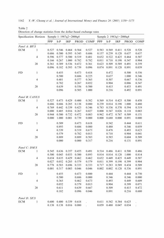
Table 2 reports the proportion of forecasts that correctly predict the direction ofthe dollar exchange rate movement and, underneath these sample proportions, the p-values for the hypothesis that the reported proportion is significantly different from1/2. When the proportion statistic is significantly larger than 1/2, the forecast is saidto have the ability to predict the direction of change. On the other hand, if the sta-tistic is significantly less than 1/2, the forecast tends to give the wrong direction ofchange. For trading purposes, information regarding the significance of incorrectprediction can be used to derive a potentially profitable trading rule by going againthe prediction generated by the model. Following this argument, one might considerthe cases in which the proportion of ‘‘correct’’ forecasts is larger than or less than 1/2contain the same information. However, in evaluating the ability of the model to de-scribe exchange rate behavior, we separate the two cases.

There is mixed evidence on the ability of the structural models to correctly predictthe direction of change. Among the 216 direction of change statistics, 50 (23) are sig-nificantly larger (less) than 1/2 at the 10% level. The occurrence of the significant out-performance cases is higher (23%) than the one implied by the 10% level of the test.


Table 2

Direction of change statistics from the dollar-based exchange rates



Panel A: BP/$

ECM 1 0.527 0.546 0.464 0.564 0.527 0.583 0.569 0.411 0.528 0.528

0.686 0.500 0.593 0.345 0.686 0.157 0.239 0.128 0.637 0.637

4 0.596 0.577 0.500 0.519 0.481 0.652 0.522 0.425 0.464 0.507

0.166 0.267 1.000 0.782 0.782 0.011 0.718 0.198 0.547 0.904

20 0.361 0.389 0.536 0.472 0.361 0.623 0.509 0.589 0.491 0.359

0.096 0.182 0.593 0.739 0.096 0.074 0.891 0.128 0.891 0.039

FD 1 0.455 0.473 0.418 0.472 0.500 0.556

0.500 0.686 0.225 0.637 1.000 0.346

4 0.481 0.577 0.365 0.507 0.667 0.536

0.782 0.267 0.052 0.904 0.006 0.547

20 0.639 0.556 0.500 0.415 0.453 0.491

0.096 0.505 1.000 0.216 0.492 0.891

Panel B: CAN$/$

ECM 1 0.527 0.473 0.429 0.400 0.382 0.569 0.514 0.425 0.500 0.458

0.686 0.686 0.285 0.138 0.080 0.239 0.814 0.198 1.000 0.480

4 0.769 0.442 0.339 0.423 0.346 0.783 0.536 0.370 0.594 0.319

0.000 0.405 0.016 0.267 0.027 0.000 0.547 0.026 0.118 0.003

20 0.944 0.500 0.732 0.472 0.083 0.962 0.472 0.767 0.509 0.151

0.000 1.000 0.001 0.739 0.000 0.000 0.680 0.000 0.891 0.000

FD 1 0.509 0.473 0.618 0.542 0.444 0.611

0.893 0.686 0.080 0.480 0.346 0.059

4 0.539 0.519 0.673 0.478 0.493 0.623

0.579 0.782 0.013 0.718 0.904 0.041

20 0.889 0.889 0.583 0.585 0.604 0.509

0.000 0.000 0.317 0.216 0.131 0.891

Panel C: DM/$

ECM 1 0.545 0.636 0.357 0.455 0.491 0.514 0.486 0.411 0.500 0.486

0.500 0.043 0.033 0.500 0.893 0.814 0.814 0.128 1.000 0.814

4 0.654 0.635 0.429 0.462 0.462 0.652 0.449 0.425 0.449 0.507

0.027 0.052 0.285 0.579 0.579 0.011 0.399 0.198 0.399 0.904

20 0.778 0.583 0.696 0.333 0.333 0.717 0.283 0.589 0.434 0.509

0.001 0.317 0.003 0.046 0.046 0.002 0.002 0.128 0.336 0.891

FD 1 0.455 0.473 0.800 0.444 0.444 0.750

0.500 0.686 0.000 0.346 0.346 0.000

4 0.365 0.462 0.673 0.493 0.449 0.609

0.052 0.579 0.013 0.904 0.399 0.071

20 0.611 0.639 0.667 0.509 0.415 0.472

0.182 0.096 0.046 0.891 0.216 0.680

Panel D: SF/$

ECM 1 0.600 0.400 0.339 0.618 . 0.611 0.542 0.384 0.625 .

0.138 0.138 0.016 0.080 . 0.059 0.480 0.047 0.034 .


The results indicate that the structural model forecasts can correctly predict the direc-tion of the change, while the proportion of cases where a random walk outperforms thecompeting models is only about what one would expect if they occurred randomly.

Let us take a closer look at the incidences in which the forecasts are in the rightdirection. Approximately 58% of the 50 cases are associated with the error correc-tion model and the remainder with the first difference specification. Thus, the errorcorrection specification e which incorporates the empirical long-run relationship eprovides a slightly better specification for the models under consideration. The fore-casting period does not have a major impact on forecasting performance, sinceexactly half of the successful cases are in each forecasting period.

Table 2 (continued)



4 0.558 0.404 0.411 0.539 . 0.638 0.580 0.425 0.580 .

0.405 0.166 0.182 0.579 . 0.022 0.185 0.198 0.185 .

20 0.750 0.444 0.455 0.583 . 0.811 0.528 0.455 0.434 .

0.003 0.505 0.670 0.317 . 0.000 0.680 0.670 0.336 .

FD 1 0.436 0.400 . 0.444 0.458 .

0.345 0.138 . 0.346 0.480 .

4 0.346 0.308 . 0.435 0.362 .

0.027 0.006 . 0.279 0.022 .

20 0.611 0.611 . 0.717 0.698 .

0.182 0.182 . 0.002 0.004 .

Panel E: Yen/$

ECM 1 0.527 0.527 0.375 0.546 . 0.597 0.597 0.425 0.514 .

0.686 0.686 0.061 0.500 . 0.099 0.099 0.198 0.814 .

4 0.673 0.577 0.482 0.519 . 0.681 0.623 0.548 0.406 .

0.013 0.267 0.789 0.782 . 0.003 0.041 0.413 0.118 .

20 0.611 0.556 0.696 0.556 . 0.811 0.415 0.703 0.340 .

0.182 0.505 0.003 0.505 . 0.000 0.216 0.001 0.020 .

FD 1 0.582 0.564 . 0.583 0.542 .

0.225 0.345 . 0.157 0.480 .

4 0.654 0.596 . 0.652 0.652 .

0.027 0.166 . 0.012 0.012 .

20 0.611 0.583 . 0.755 0.736 .

0.182 0.317 . 0.000 0.001 .

Note: Table 3 reports the proportion of forecasts that correctly predict the direction of the dollar exchange

rate movement. Underneath each direction of change statistic, the p-values for the hypothesis that the re-

ported proportion is significantly different from 1/2 is listed. When the statistic is significantly larger than

1/2, the forecast is said to have the ability to predict the direction of change. If the statistic is significantly

less than 1/2, the forecast tends to give the wrong direction of change. The notations used in the table are

ECM: error correction specification; FD: first-difference specification; PPP: purchasing power parity mod-

el; S-P: sticky-price model; IRP: interest rate parity model; PROD: productivity differential model; and

COMP: composite model. The forecasting horizons (in quarters) are listed under the heading ‘‘Horizon.’’

The results for the post-Louvre Accord forecasting period are given under the label ‘‘Sample 1’’ and those

for the post-1983 forecasting period are given under the label ‘‘Sample 2.’’ A ‘‘.’’ indicates the statistics are

not generated due to unavailability of data.


Among the five models under consideration, the purchasing power parity specifi-cation has the highest number (18) of forecasts that give the correct direction ofchange prediction, followed by the sticky-price, composite, and productivity models(10, 9, and 8, respectively), and the interest rate parity model (5). Thus, at least onthis count, the newer exchange rate models do not edge out the ‘‘old fashioned’’ pur-chasing power parity doctrine and the sticky-price model. Because there are differingnumbers of forecasts due to data limitations and specifications, the proportions donot exactly match up with the numbers. Proportionately, the purchasing power modeldoes the best.

Interestingly, the success of direction of change prediction appears to be currencyspecific. The dollareyen exchange rate yields 13 out of 50 forecasts that give the cor-rect direction of change prediction. In contrast, the dollarepound has only four outof 50 forecasts that produce the correct direction of change prediction.

The cases of correct direction prediction appear to cluster at the long forecast ho-rizon. The 20-quarter horizon accounts for 22 of the 50 cases while the 4- and 1-quarter horizons have 18 and 10 direction of change statistics, respectively, thatare significantly larger than 1/2. Since there have not been many studies utilizingthe direction of change statistic in similar contexts, it is difficult to make compari-sons. Chinn and Meese (1995) apply the direction of change statistic to 3-year hori-zons for three conventional models, and find that performance is largely currencyspecific: the no change prediction is outperformed in the case of the dollareyen ex-change rate, while all models are outperformed in the case of the dollarepound rate.In contrast, in our study at the 20-quarter horizon, the positive results appear to befairly evenly distributed across the currencies, with the exception of the dollarepound rate.13 Mirroring the MSE results, it is interesting to note that the directionof change statistic works for the purchasing power parity at the 4- and 20-quarterhorizons and for the interest rate parity model only at the 20-quarter horizon.This pattern is entirely consistent with the findings that the two parity conditionshold better at long horizons.14

4.3. The consistency criterion

The consistency criterion only requires the forecast and actual realization comoveone-to-one in the long run. In assessing the consistency, we first test if the forecastand the realization are cointegrated.15 If they are cointegrated, then we test if the

13 Using Markov switching models, Engel (1994) obtains some success along the direction of change di-

mension at horizons of up to 1 year. However, his results are not statistically significant.14 Flood and Taylor (1997) noted the tendency for PPP to hold better at longer horizons. Mark and Moh

(2001) document the gradual currency appreciation in response to a short-term interest differential, con-

trary to the predictions of uncovered interest parity.15 The Johansen method is used to test the null hypothesis of no cointegration. The maximum eigenvalue

statistics are reported in the manuscript. Results based on the trace statistics are essentially the same. Be-

fore implementing the cointegration test, both the forecast and exchange rate series were checked for the

I(1) property. For brevity, the I(1) test results and the trace statistics are not reported.


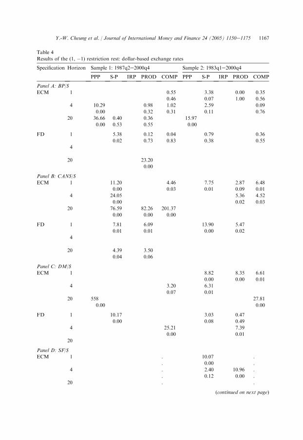
cointegrating vector satisfies the (1, �1) requirement. The cointegration results are re-ported in Table 3, while the test results for the (1,�1) restriction are reported in Table 4.

In Table 3, 67 of 216 cases reject the null hypothesis of no cointegration at the 10%significance level. Thus, 67 forecast series (31% of the total number) are cointegratedwith the corresponding spot exchange rates. The error correction specification ac-counts for 39 of the 67 cointegrated cases and the first-difference specification accountsfor the remaining 28 cases. There is some evidence that the error correction specifica-tion gives better forecasting performance than the first-difference specification. These67 cointegrated cases are slightly more concentrated in the longer of the two forecast-ing periods e 30 for the post-Louvre Accord period and 37 for the post-1983 period.

Interestingly, the sticky-pricemodel garners the largest number of cointegrated cases.There are 60 forecast series generated under the sticky-price model. Twenty-six of these60 series (i.e. 43%) are cointegrated with the corresponding spot rates. The compositemodel has the second highest frequency of cointegrated forecast series e 39% of 36 se-ries. Thirty-seven percent of the productivity differential model forecast series, 33% ofthe purchasing power parity model, and none of the interest rate parity model are co-integrated with the spot rates. Apparently, we do not find evidence that the recently de-veloped exchange rate models outperform the ‘‘old’’ vintage sticky-price model.

The dollarepound and dollareCanadian dollar, each have between 19 and 17forecast series that are cointegrated with their respective spot rates. The dollaremark pair, which yields relatively good forecasts according to the direction of changemetric, has only 12 cointegrated forecast series. Evidently, the forecasting perfor-mance is not just currency specific; it also depends on the evaluation criterion.The distribution of the cointegrated cases across forecasting horizons is puzzling.The frequency of occurrence is inversely proportional to the forecasting horizons.There are 35 of 67 one-quarter ahead forecast series that are cointegrated with thespot rates. However, there are only 20 of the 4-quarter ahead and 12 of the 20-quar-ter ahead forecast series that are cointegrated with the spot rates. One possible expla-nation for this result is that there are fewer observations in the 20-quarter aheadforecast series and this affects the power of the cointegration test.

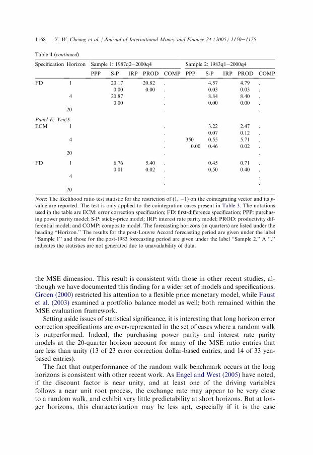
The results of testing for the long-run unitary elasticity of expectations at the 10%sig-nificance level are reported in Table 4. The condition of long-run unitary elasticity of ex-pectationse that is the (1,�1) restriction on the cointegrating vectore is rejected by thedata quite frequently: 48 of the 67 cointegration cases. That is 28% of the cointegratedcases display long-run unitary elasticity of expectations. Taking both the cointegrationand restriction test results together, 9% of the 216 cases of the dollar-based exchangerate forecast series meet the consistency criterion. A slightly higher proportion(12%)meet the consistency criterion in the case of the yen-based exchange rates (resultsnot reported), but the pattern is essentially the same as for the dollar-based exchangerates.

4.4. Discussion

Several aspects of the foregoing analysis merit discussion. To begin with, even atlong horizons, the performance of the structural models is less than impressive along

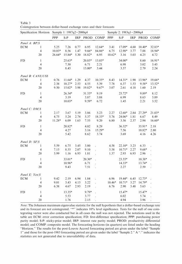
Table 3

Cointegration between dollar-based exchange rates and their forecasts



Panel A: BP/$

ECM 1 5.25 7.26 0.77 6.95 12.64* 3.41 17.09* 4.60 10.40* 32.83*

4 10.03* 8.56 1.47 9.66* 84.86* 6.75 12.98* 3.77 7.88 18.94*

20 26.64* 15.84* 5.30 18.82* 6.95 10.62* 3.16 5.03 4.25 4.72

FD 1 25.63* 20.85* 13.03* 34.00* 8.60 16.91*

4 7.30 6.71 2.21 6.98 3.02 3.45

20 8.45 13.00* 3.44 3.57 2.79 2.24

Panel B: CAN$/US$

ECM 1 0.76 11.64* 1.29 4.37 10.35* 8.43 14.31* 1.90 13.96* 19.66*

4 2.38 10.27* 2.53 4.55 5.39 7.78 6.37 1.53 9.58* 13.52*

20 9.50 15.02* 3.98 19.82* 9.67* 3.07 2.61 4.18 1.60 2.19

FD 1 26.34* 31.53* 9.19 25.72* 9.89* 8.12

4 3.19 3.87 3.88 6.99 8.63 3.89

20 10.03* 9.59* 6.72 1.45 2.21 3.52

Panel C: DM/$

ECM 1 2.17 3.67 5.19 3.86 5.23 2.27 12.68* 2.84 27.29* 21.03*

4 4.75 5.24 2.74 5.37 18.33* 5.76 24.06* 1.81 6.67 8.49

20 11.28* 6.09 1.63 7.55 9.20 6.80 3.56 2.37 2.94 16.60*

FD 1 20.82* 4.02 8.29 36.32* 35.91* 2.18

4 4.27 3.16 15.29* 7.56 10.82* 2.80

20 5.42 8.62 3.74 3.69 4.16 4.26

Panel D: SF/$

ECM 1 5.59 6.75 3.45 3.80 . 4.58 22.10* 3.23 6.33 .

4 7.15 8.55 2.07 9.10 . 5.58 10.71* 2.27 9.68* .

20 5.99 1.16 6.93 1.81 . 1.37 2.93 6.93 2.96 .

FD 1 33.01* 20.30* . 23.55* 10.38* .

4 10.96* 6.71 . 14.33* 13.74* .

20 9.43 7.51 . 2.27 2.59 .

Panel E: Yen/$

ECM 1 9.42 2.19 6.94 1.84 . 6.96 19.44* 6.45 12.73* .

4 9.01 3.43 4.13 3.22 . 10.46* 10.71* 3.27 14.79* .

20 6.38 4.67 2.93 2.19 . 6.76 2.90 3.48 5.63 .

FD 1 13.35* 9.79* . 15.47* 15.47* .

4 5.53 3.77 . 6.02 5.74 .

20 1.76 2.15 . 4.94 3.96 .

Note: The Johansen maximum eigenvalue statistic for the null hypothesis that a dollar-based exchange rate

and its forecast are not cointegrated. ‘‘*’’ indicates 10% level significance. Tests for the null of one coin-

tegrating vector were also conducted but in all cases the null was not rejected. The notations used in the

table are ECM: error correction specification; FD: first-difference specification; PPP: purchasing power

parity model; S-P: sticky-price model; IRP: interest rate parity model; PROD: productivity differential

model; and COMP: composite model. The forecasting horizons (in quarters) are listed under the heading

‘‘Horizon.’’ The results for the post-Louvre Accord forecasting period are given under the label ‘‘Sample

1’’ and those for the post-1983 forecasting period are given under the label ‘‘Sample 2.’’ A ‘‘.’’ indicates the

statistics are not generated due to unavailability of data.


Table 4

Results of the (1, �1) restriction rest: dollar-based exchange rates



Panel A: BP/$

ECM 1 0.55 3.38 0.00 0.35

0.46 0.07 1.00 0.56

4 10.29 0.98 1.02 2.59 0.09

0.00 0.32 0.31 0.11 0.76

20 36.66 0.40 0.36 15.97

0.00 0.53 0.55 0.00

FD 1 5.38 0.12 0.04 0.79 0.36

0.02 0.73 0.83 0.38 0.55

4

20 23.20

0.00

Panel B: CAN$/$

ECM 1 11.20 4.46 7.75 2.87 6.48

0.00 0.03 0.01 0.09 0.01

4 24.05 5.36 4.52

0.00 0.02 0.03

20 76.59 82.26 201.37

0.00 0.00 0.00

FD 1 7.81 6.09 13.90 5.47

0.01 0.01 0.00 0.02

4

20 4.39 3.50

0.04 0.06

Panel C: DM/$

ECM 1 8.82 8.35 6.61

0.00 0.00 0.01

4 3.20 6.31

0.07 0.01

20 558 27.81

0.00 0.00

FD 1 10.17 3.03 0.47

0.00 0.08 0.49

4 25.21 7.39

0.00 0.01

20

Panel D: SF/$

ECM 1 . 10.07 .

. 0.00 .

4 . 2.40 10.96 .

. 0.12 0.00 .

20 . .

(continued on next page)


the MSE dimension. This result is consistent with those in other recent studies, al-though we have documented this finding for a wider set of models and specifications.Groen (2000) restricted his attention to a flexible price monetary model, while Faustet al. (2003) examined a portfolio balance model as well; both remained within theMSE evaluation framework.

Setting aside issues of statistical significance, it is interesting that long horizon errorcorrection specifications are over-represented in the set of cases where a random walkis outperformed. Indeed, the purchasing power parity and interest rate paritymodels at the 20-quarter horizon account for many of the MSE ratio entries thatare less than unity (13 of 23 error correction dollar-based entries, and 14 of 33 yen-based entries).

The fact that outperformance of the random walk benchmark occurs at the longhorizons is consistent with other recent work. As Engel and West (2005) have noted,if the discount factor is near unity, and at least one of the driving variablesfollows a near unit root process, the exchange rate may appear to be very closeto a random walk, and exhibit very little predictability at short horizons. But at lon-ger horizons, this characterization may be less apt, especially if it is the case

Table 4 (continued)



FD 1 20.17 20.82 . 4.57 4.79 .

0.00 0.00 . 0.03 0.03 .

4 20.87 . 8.84 8.40 .

0.00 . 0.00 0.00 .

20 . .

Panel E: Yen/$

ECM 1 . 3.22 2.47 .

. 0.07 0.12 .

4 . 350 0.55 5.71 .

. 0.00 0.46 0.02 .

20 . .

FD 1 6.76 5.40 . 0.45 0.71 .

0.01 0.02 . 0.50 0.40 .

4 . .

. .

20 . .

Note: The likelihood ratio test statistic for the restriction of (1, �1) on the cointegrating vector and its p-

value are reported. The test is only applied to the cointegration cases present in Table 3. The notations

used in the table are ECM: error correction specification; FD: first-difference specification; PPP: purchas-

ing power parity model; S-P: sticky-price model; IRP: interest rate parity model; PROD: productivity dif-

ferential model; and COMP: composite model. The forecasting horizons (in quarters) are listed under the

heading ‘‘Horizon.’’ The results for the post-Louvre Accord forecasting period are given under the label

‘‘Sample 1’’ and those for the post-1983 forecasting period are given under the label ‘‘Sample 2.’’ A ‘‘.’’

indicates the statistics are not generated due to unavailability of data.


that exchange rates are not weakly exogenous with respect to the cointegratingvector.16

Expanding the set of criteria does yield some interesting surprises. In particular,the direction of change statistics indicates more evidence that structural modelscan outperform a random walk. However, the basic conclusion that no specific eco-nomic model is consistently more successful than the others remains intact. This, webelieve, is a new finding.17

Even if we cannot glean from this analysis a consistent ‘‘winner’’, it may still be ofinterest to note the best and worst performing combinations of model/specification/currency. Of the reported results, the interest rate parity model at the 20-quarter ho-rizon for the dollareyen exchange rate (post-1982) performs best according to theMSE criterion, with an MSE ratio of 0.57 ( p-value of 0.17). (The corresponding re-sults for the Canadian dollareyen exchange rate are even better, with a ratio of 0.48( p-value of 0.04); see Cheung et al., 2003, Table 2.)

Note, however, that the superior performance of a particular model/specification/currency combination does not necessarily carry over from one out-of-sample periodto the other. That is the lowest dollar-based MSE ratio during the 1987q2e2000q4period is for the Deutsche mark composite model in first differences, while the cor-responding entry for the 1983q1e2000q4 period is for the yen interest parity model.

Aside from the purchasing power parity specification, the worst performances areassociated with first-difference specifications; in this case the highest MSE ratio isfor the first-difference specification of the composite model at the 20-quarter horizonfor the poundedollar exchange rate over the post-Louvre period. However, the othercatastrophic failures in prediction performance are distributed across the various mod-els estimated in first differences, so (taking into account the fact that these predictionsutilize ex post realizations of the right-hand-side variables) the key determinant in thispattern of results appears to be the difficulty in estimating stable short-run dynamics.

That being said, we do not wish to overplay the stability of the long-run estimateswe obtain. In a companion study (Cheung et al., 2005), we do not find a definite re-lationship between in-sample fit and out-of-sample forecast performance. Moreover,the estimates exhibit wide variation over time. Even in cases where the structuralmodel does reasonably well, there is quite substantial time-variation in the estimateof the rate at which the exchange rate responds to disequilibria. A similar observa-tion applies to the coefficient estimates of the parameters of the cointegrating vector.Thus, an interesting future research topic is to further investigate the effect of impos-ing parameter restrictions and the interaction between parameter instability andforecast performance.

16 Engel and West (2005) use Granger causality tests to conduct their inference. Since they fail to find

cointegration of the exchange rate with the monetary fundamentals, they do not conduct tests for weak

exogeneity. However, other studies, spanning different sample periods and models, have detected both co-

integration; see for instance MacDonald and Marsh (1999) and Chinn (1997), among others.17 An interesting research topic, as suggested by a referee, is to investigate whether the forecasts of these

models can generate profitable trading strategies. The issue, which is beyond the scope of the current ex-

ercise, would involve obtaining different vintages of macro data to use as future variables in generating

forecasts.


One question that might occur to the reader is whether our results are sensitive tothe out-of-sample period we have selected. In fact, it is possible to improve the per-formance of the models according to an MSE criterion by selecting a shorter out-of-sample forecasting period. In another set of results (Cheung et al., 2005), we imple-mented the same exercises for a 1993q1e2000q4 forecasting period, and found some-what greater success for dollar-based rates according to the MSE criterion, andsomewhat less success along the direction of change dimension. We believe thatthe difference in results is an artifact of the long upswing in the dollar during the1990s that gives an advantage to structural models over the no-change forecast em-bodied in the random walk model when using the most recent 8 years of the floatingrate period as the prediction sample. This conjecture is buttressed by the fact that theyen-based exchange rates did not exhibit a similar pattern of results. Thus, in usingfairly long out-of-sample periods, as we have done, we have given maximum advan-tage to the random walk characterization.

5. Concluding remarks

This paper has systematically assessed the predictive capabilities of models devel-oped during the 1990s. These models have been compared along a number of dimen-sions, including econometric specification, currencies, out-of-sample predictionperiods, and differing metrics. The differences in forecast evaluations from differentevaluation criteria, for instance, illustrate the potential limitation of using a singlecriterion such as the popular MSE metric. Clearly, the evaluation criteria couldhave been expanded further. For instance, recently Abhyankar et al. (2005) haveproposed a utility-based metric based upon the portfolio allocation problem. Theyfind that the relative performance of the structural model increases when usingthis metric. To the extent that this is a general finding, one can interpret our ap-proach as being conservative with respect to finding superior model performance.18

At this juncture, it may also be useful to outline the boundaries of this study withrespect to models and specifications. Firstly, we have only evaluated linear models,eschewing functional nonlinearities (Meese and Rose, 1991; Kilian and Taylor, 2003)and regime switching (Engel and Hamilton, 1990; Cheung and Erlandsson, 2005).Nor have we employed panel regression techniques in conjunction with long-run re-lationships, despite the fact that recent evidence suggests the potential usefulness ofsuch approaches (Mark and Sul, 2001). Further, we did not undertake systems-basedestimation that has been found in certain circumstances to yield superior forecastperformance, even at short horizons (e.g., MacDonald and Marsh, 1997). Sucha methodology would have proven much too cumbersome to implement in thecross-currency recursive framework employed in this study. Finally, the currentstudy examines the forecasting performance and the results are not necessarily indic-ative of the abilities of these models to explain exchange rate behavior. For instance,

18 McCracken and Sapp (2005) forward an encompassing test for nested models. Since not all of our

models can be nested in a general specification, we do not implement this approach.


Clements and Hendry (2001) show that an incorrect but simple model may outper-form a correct model in forecasting. Consequently, one could view this exercise asa first pass examination of these newer exchange rate models.

In summarizing the evidence from this extensive analysis, we conclude that the an-swer to the question posed in the title of this paper is a bold ‘‘perhaps.’’ That is, theresults do not point to any given model/specification combination as being very suc-cessful. On the other hand, some models seem to do well at certain horizons, for cer-tain criteria. And indeed, it may be that one model will do well for one exchange rate,and not for another. For instance, the productivity model does well for the markeyen rate along the direction of change and consistency dimensions (although not bythe MSE criterion); but that same conclusion cannot be applied to any other ex-change rate. Perhaps it is in this sense that the results from this study set the stagefor future research.

Acknowledgements

We thank, without implicating, two anonymous referees, Mario Crucini, CharlesEngel, Jeff Frankel, Fabio Ghironi, Jan Groen, Lutz Kilian, Ed Leamer, RonaldMacDonald, Nelson Mark, Mike Melvin (Co-Editor), David Papell, Roberto Rigo-bon, John Rogers, Lucio Sarno, Torsten Sløk, Mark Taylor, Frank Westermann,seminar participants at Academica Sinica, the Bank of England, Boston College,UCLA, University of Houston, University of Wisconsin, Brandeis University, theECB, Kiel, Federal Reserve Bank of Boston, and conference participants at theNBER Summer Institute, the CES-ifo Venice Summer Institute conference on ‘‘Ex-change Rate Modeling’’ and the 2003 IEFS panel on international finance for helpfulcomments and suggestions. Jeannine Bailliu, Gabriele Galati and Guy Meredith gra-ciously provided data. The financial support of faculty research funds of the Univer-sity of California, Santa Cruz is gratefully acknowledged. The views containedherein do not necessarily represent those of the IMF or any other organizationsthe authors are associated with.

Appendix 1. Data

Unless otherwise stated, we use seasonally adjusted quarterly data from the IMFInternational Financial Statistics ranging from the second quarter of 1973 to the lastquarter of 2000. The exchange rate data are end-of-period exchange rates. The out-put data are measured in constant 1990 prices. The consumer and producer price in-dices also use 1990 as base year. Inflation rates are calculated as 4-quarter logdifferences of the CPI. Real interest rates are calculated by subtracting the lagged in-flation rate from the 3-month nominal interest rates.

The 3-month, annual and 5-year interest rates are end-of-period constant maturityinterest rates, and are obtained from the IMF country desks. See Chinn andMeredith (2004) for details. Five-year interest rate data were unavailable for


Japan and Switzerland; hence data from Global Financial Data http://www.global-findata.com/ were used, specifically, 5-year government note yields for Switzerlandand 5-year discounted bonds for Japan.

The productivity series are labor productivity indices, measured as real GDP peremployee, converted to indices (1995Z 100). These data are drawn from the Bankfor International Settlements database.

The net foreign asset (NFA) series is computed as follows. Using stock data foryear 1995 on NFA (Lane and Milesi-Ferretti, 2001) at http://econserv2.bess.tcd.ie/plane/data.html, and flow quarterly data from the IFS statistics on the current ac-count, we generated quarterly stocks for the NFA series (with the exception of Ja-pan, for which there is no quarterly data available on the current account).

To generate quarterly government debt data we follow a similar strategy. We useannual debt data from the IFS statistics, combined with quarterly government deficit(surplus) data. The data source for Canadian government debt is the Bank of Can-ada. For the UK, the IFS data are updated with government debt data from the pub-lic sector accounts of the UK Statistical Office (for Japan and Switzerland we havevery incomplete data sets, and hence no composite models are estimated for thesetwo countries).

Appendix 2. Evaluating forecast accuracy

The DieboldeMariano statistics (Diebold and Mariano, 1995) are used to evalu-ate the forecast performance of the different model specifications relative to that ofthe naive random walk. Given the exchange rate series xt and the forecast series yt,the loss function L for the mean square error is defined as:

LðytÞZðyt � xtÞ2: ðA1Þ

Testing whether the performance of the forecast series is different from that of thenaive random walk forecast zt, it is equivalent to testing whether the populationmean of the loss differential series dt is zero. The loss differential is defined as

dtZLðytÞ �LðztÞ: ðA2Þ

Under the assumptions of covariance stationarity and short-memory for dt, thelarge-sample statistic for the null of equal forecast performance is distributed asa standard normal, and can be expressed as

�d

(2p

XðT�1Þ

tZ�ðT�1Þlðt=SðTÞÞ

XTtZjtjC1

ðdt � �dÞ�dt�jtj � �d Þ

)�1=2

; ðA3Þ

where lðt=SðTÞÞ is the lag window, S(T ) is the truncation lag, and T is the number ofobservations. Different lag-window specifications can be applied, such as the Barlett

http://www.globalfindata.com/

http://www.globalfindata.com/

http://econserv2.bess.tcd.ie/plane/data.html

http://econserv2.bess.tcd.ie/plane/data.html


or the quadratic spectral kernels, in combination with a data-dependent lag-selectionprocedure (Andrews, 1991).

For the direction of change statistic, the loss differential series is defined as fol-lows: dt takes a value of one if the forecast series correctly predicts the directionof change, otherwise it will take a value of zero. Hence, a value of �d significantly larg-er than 0.5 indicates that the forecast has the ability to predict the direction ofchange; on the other hand, if the statistic is significantly less than 0.5, the forecasttends to give the wrong direction of change. In large samples, the studentized versionof the test statistic,

ð�d� 0:5Þ=ffiffiffiffiffiffiffiffiffiffiffiffiffiffiffi0:25=T

p; ðA4Þ

is distributed as a standard Normal.

References

Abhyankar, A., Sarno, L., Valente, G., 2005. Exchange rates and fundamentals: evidence on the economic

value of predictability. Journal of International Economics 66, 325e348.

Alberola, E., Cervero, S., Lopez, H., Ubide, A., 1999. Global equilibrium exchange rates: euro, dollar,

‘ins’, ‘outs’, and other major currencies in a panel cointegration framework. IMF Working Paper

99/175.

Alexius, A., 2001. Uncovered interest parity revisited. Review of International Economics 9, 505e517.

Andrews, D., 1991. Heteroskedasticity and autocorrelation consistent covariance matrix estimation. Econ-

ometrica 59, 817e858.Cavallo, M., Ghironi, F., 2002. Net foreign assets and the exchange rate: redux revived. Journal of Mon-

etary Economics 49, 1057e1097.

Cheung, Y.-W., Chinn, M.D., 1998. Integration, cointegration, and the forecast consistency of structural

exchange rate models. Journal of International Money and Finance 17, 813e830.

Cheung, Y.-W., Chinn, M.D., Garcia Pascual, A., 2003. Empirical exchange rate models of the nineties:

are any fit to survive? Working Paper No. 551, University of California, Santa Cruz.

Cheung, Y.-W., Chinn, M.D., Garcia Pascual, A., 2005. What do we know about recent exchange rate

models? In-sample fit and out-of-sample performance evaluated. In: DeGrauwe, P. (Ed.), Exchange

Rate Modelling: Where Do We Stand? MIT Press for CESIfo, Cambridge, MA, pp. 239e276.

Cheung, Y.-W., Erlandsson, U.G., 2005. Exchange rates and Markov switching dynamics. Journal of

Business and Economic Statistics 23, 314e320.Chinn, M.D., 1997. Paper pushers or paper money? Empirical assessment of fiscal and monetary models of

exchange rate determination. Journal of Policy Modeling 19, 51e78.

Chinn, M.D., Meese, R.A., 1995. Banking on currency forecasts: how predictable is change in money?’’.

Journal of International Economics 38, 161e178.

Chinn, M.D., Meredith, G., 2004. Monetary policy and long horizon uncovered interest parity. IMF Staff

Papers 51, 409e430.

Christoffersen, P.F., Diebold, F.X., 1998. Cointegration and long-horizon forecasting. Journal of Business

and Economic Statistics 16, 450e458.

Clark, P., MacDonald, R., 1999. Exchange rates and economic fundamentals: a methodological compar-

ison of Beers and Feers. In: Stein, J., MacDonald, R. (Eds.), Equilibrium Exchange Rates. Kluwer,

Boston, MA, pp. 285e322.Clements, K., Frenkel, J., 1980. Exchange rates, money and relative prices: the dollarepound in the 1920s.


Clements, M.P., Hendry, D.F., 2001. Forecasting with difference and trend stationary models. The Econo-

metric Journal 4, S1eS19.


Clostermann, J., Schnatz, B., 2000. The determinants of the euroedollar exchange rate: synthetic funda-

mentals and a non-existent currency. Discussion Paper 2/00, Deutsche Bundesbank, Frankfurt.

Cumby, R.E., Modest, D.M., 1987. Testing for market timing ability: a framework for forecast evaluation.

Journal of Financial Economics 19, 169e189.

DeGregorio, J., Wolf, H., 1994. Terms of trade, productivity, and the real exchange rate. NBER Working

Paper No. 4807.

Dornbusch, R., 1976. Expectations and exchange rate dynamics. Journal of Political Economy 84, 1161e1176.

Diebold, F.X., Mariano, R., 1995. Comparing predictive accuracy. Journal of Business and Economic Sta-

tistics 13, 253e265.

Economist, 7 April 2001. Finance and economics: the darling dollar. Economist, 81e82.Edwards, S., 1989. Real Rates, Devaluation and Adjustment. MIT Press, Cambridge, MA.

Engel, C., 1994. Can the Markov switching model forecast exchange rates? Journal of International Eco-

nomics 36, 151e165.Engel, C., Hamilton, J., 1990. Long swings in the exchange rate: are they in the data and do markets know

it? American Economic Review 80, 689e713.

Engel, C., West, K.D., 2005. Exchange rates and fundamentals. Journal of Political Economy 113, 485e

517.

Faruqee, H., Isard, P., Masson, P.R., 1999. A macroeconomic balance framework for estimating equilib-

rium exchange rates. In: Stein, J., MacDonald, R. (Eds.), Equilibrium Exchange Rates. Kluwer, Bos-

ton, MA, pp. 103e134.

Faust, J., Rogers, J., Wright, J., 2003. Exchange rate forecasting: the errors we’ve really made. Journal of

International Economics 60, 35e60.

Flood, R.P., Taylor, M.P., 1997. Exchange rate economics: what’s wrong with the conventional macro

approach? In: Frankel, J., Galli, G., Giovannini, A. (Eds.), The Microstructure of Foreign Exchange

Markets University of Chicago Press for NBER, Chicago, pp. 262e301.

Frankel, J.A., 1979. On the mark: a theory of floating exchange rates based on real interest differentials.

American Economic Review 69, 610e622.

Frankel, J.A., 1985. The dazzling dollar. Brookings Papers on Economic Activity 1985, 199e217.Groen, J.J.J., 2000. The monetary exchange rate model as a long-run phenomenon. Journal of Interna-

tional Economics 52, 299e320.

Inoue, A., Kilian, L., 2004. In-sample or out-of-sample tests of predictability: which one should we use?

Econometric Reviews 23, 371e402.Kilian, L., Taylor, M.P., 2003. Why is it so difficult to beat the random walk forecast of exchange rates?


Lane, P., Milesi-Ferretti, G.M., 2001. The external wealth of nations: measures of foreign assets and lia-

bilities for industrial and developing. Journal of International Economics 55, 263e294.

Leitch, G., Tanner, J.E., 1991. Economic forecast evaluation: profits versus the conventional error meas-

ures. American Economic Review 81, 580e590.

Lucas, R.E., 1982. Interest rates and currency prices in a two-country world. Journal of Monetary Eco-

nomics 10, 335e359.

McCracken, M., Sapp, S., 2005. Evaluating the predictability of exchange rates using long horizon regres-

sion. Journal of Money, Credit and Banking 37, 473e494.

MacDonald, R., Marsh, I., 1997. On fundamentals and exchange rates: a Casselian perspective. Review of

Economics and Statistics 79, 655e664.

MacDonald, R., Marsh, I., 1999. Exchange Rate Modeling. Kluwer, Boston.

MacDonald, R., Nagayasu, J., 2000. The long-run relationship between real exchange rates and real in-

terest rate differentials. IMF Staff Papers 47, 116e128.Mark, N., 1995. Exchange rates and fundamentals: evidence on long horizon predictability. American

Economic Review 85, 201e218.

Mark, N., Moh, Y.-K., 2001. What do interest-rate differentials tell us about the exchange rate?

Paper presented at conference on ‘‘Empirical Exchange Rate Models,’’ University of Wisconsin,

Madison.


Mark, N., Sul, D., 2001. Nominal exchange rates and monetary fundamentals: evidence from a small post-

Bretton Woods panel. Journal of International Economics 53, 29e52.

Meese, R., Rogoff, K., 1983. Empirical exchange rate models of the seventies: do they fit out of sample?


Meese, R., Rose, A.K., 1991. An empirical assessment of non-linearities in models of exchange rate deter-

mination. Review of Economic Studies 58, 603e619.

Obstfeld, M., Rogoff, K., 1995. Exchange rate dynamics redux. Journal of Political Economy 91, 675e687.

Owen, D., 2001. Importance of productivity trends for the euro, European economics for investors.

DresdnerKleinwortWasserstein.

Rosenberg, M., 2001. Investment strategies based on long-dated forward rate/PPP divergence, FXWeekly.

Deutsche Bank Global Markets Research, New York, pp. 4e8.

Rosenberg, M., 2000. The euro’s long-term struggle. FX Research Special Report Series, No. 2. Deutsche

Bank, London.

Schnatz, B., Vijselaar, F., Osbat, C., 2004. Productivity and the (‘synthetic’) euroedollar exchange rate.

Review of World Economics 140, 1e30.

Stein, J., 1999. The evolution of the real value of the US dollar relative to the G7 currencies. In: Stein, J.,

MacDonald, R. (Eds.), Equilibrium Exchange Rates. Kluwer, Boston, pp. 67e102.Stockman, A., 1980. A theory of exchange rate determination. Journal of Political Economy 88, 673e698.

Yilmaz, F., 2003. Currency alert: EUR valuationdpart I. Bank of America, London.

Yilmaz, F., Jen, S., 2001. Correcting the US Dollar e a technical note. Morgan Stanley Dean Witter.

empirical exchange rate models of the nineties: are …mchinn/ccg-p_jimf.pdf2 meese and rogoﬀ...

Documents