emission functions for heavy duty vehicles be-223
TRANSCRIPT
EMISSION FUNCTIONS FOR
HEAVY DUTY VEHICLES
Update of the Emission Functions for Heavy Duty Vehicles in the Handbook Emission
Factors for Road Traffic
BE
-223

EMISSION FUNCTIONS FOR
HEAVY DUTY VEHICLES
Update of the Emission Functions
for Heavy Duty Vehicles in the Handbook
Emission Factors for Road Traffic
Institute for Internal Combustion Engines and Thermodynamics
Graz University of Technology
Univ.-Prof. Dr. Rudolf Pischinger
Elaborated by:
DI Dr. Stefan Hausberger
DI Dieter Engler
DI Mario Ivanisin
DI Martin Rexeis
Elaborated in order of:
Federal Environment Agency - Austria
Federal Ministry of Agriculture, Forestry, Environment and WaterManagement
Federal Ministry of Transport, Innovation and Technology
Project manager: DI Günther Lichtblau Federal Environment Agency Austria
BE-223
Vienna, February 2003
The study was financed by:
Federal Environment Agency - AustriaDept. Environmental Management, Traffic and Noise Dr. Elisabeth Friedbacher (Head of Department)
Federal Ministry of Agriculture, Forestry, Environment and Water Management Division V/5; Transport, Mobility, Human Settlement and Noise DI. Robert Thaler (Head of Department)
Federal Ministry of Transport, Innovation and Technology Division I/7; Mobility and Transport Technology Mag. Evelinde Grassegger (Head of Department)
Further information concerning publications of the Federal Environment Agency Ltd. can be found at: http://www.ubavie.gv.at
Impressum
Editor: Umweltbundesamt GmbH (Federal Environment Agency Ltd.) Spittelauer Lände 5, A-1090 Vienna, Austria
© Umweltbundesamt GmbH, Vienna, February 2003 All rights reserved ISBN 3-85457-679-X
Emission Functions for Heavy Duty Vehicles 1
Federal Environment Agency – Austria BE-223 (2003)
CONTENTS :
ZUSAMMENFASSUNG .............................................................................................................. 3
1 EXECUTIVE SUMMARY...................................................................................................... 7
2 INTRODUCTION.................................................................................................................. 11
3 APPROACH ........................................................................................................................... 11
4 DATA USED........................................................................................................................... 13
4.1 Engine test bed, steady state measurements ........................................................................ 15 4.1.1 SETTING OF THE SEQUENCE AND DURATION OF MEASUREMENT....................................................19 4.1.2 REPEATABILITY OF THE STEADY STATE MEASUREMENTS..............................................................22 4.1.3 ASSESSMENT OF THE STEADY STATE MEASUREMENTS ..................................................................23
4.2 Engine test bed, transient measurements ............................................................................. 28 4.2.1 ASSESSMENT OF THE TRANSIENT ENGINE TESTS ............................................................................30
4.3 Chassis dynamometer measurements .................................................................................. 34
5 THE HDV EMISSION MODEL .......................................................................................... 36
5.1 Simulation of the engine power ........................................................................................... 385.1.1 POWER FOR OVERCOMING THE ROLLING RESISTANCE ...................................................................39 5.1.2 POWER FOR OVERCOMING THE AIR RESISTANCE............................................................................41 5.1.3 POWER FOR ACCELERATION ...........................................................................................................42 5.1.4 POWER FOR OVERCOMING ROAD GRADIENTS.................................................................................43 5.1.5 POWER DEMAND OF AUXILIARIES...................................................................................................43 5.1.6 POWER DEMAND OF THE TRANSMISSION SYSTEM ..........................................................................43
5.2 Simulation of the engine speed............................................................................................ 46
5.3 Interpolation from the engine emission map ....................................................................... 49 5.3.1 THE INTERPOLATION ROUTINE .......................................................................................................49 5.3.2 STANDARD FORMATS FOR THE EMISSION MAPS .............................................................................52
5.4 Simulation of transient cycles.............................................................................................. 57 5.4.1 COMPARISON OF MEASURED EMISSIONS AND INTERPOLATION RESULTS FROM ENGINE MAPS ......57 5.4.2 THE TRANSIENT CORRECTION FUNCTIONS......................................................................................59
5.5 HDV Emission Model Accuracy ......................................................................................... 64 5.5.1 INFLUENCE OF THE ENGINE SAMPLE...............................................................................................65 5.5.2 ACCURACY OF SIMULATING TRANSIENT ENGINE TESTS.................................................................66 5.5.3 ACCURACY OF SIMULATING HDV DRIVING CYCLES......................................................................74
6 EMISSION MAPS FOR EURO 4 AND EURO 5 ............................................................... 84
6.1 Technologies under consideration ....................................................................................... 86 6.1.1 DIESEL PARTICULATE FILTER (DPF)..............................................................................................86 6.1.2 NOX CATALYSTS.............................................................................................................................896.1.3 EXHAUST GAS RECIRCULATION (EGR) .........................................................................................89
6.2 Estimation of EURO 4 and EURO 5 emission maps........................................................... 91
6.3 Average Emission Maps for Pre EURO to EURO 5 ........................................................... 92
2 Emission Functions for Heavy Duty Vehicles
BE-223 (2003) Federal Environment Agency – Austria
7 CALCULATION OF THE EMISSION FACTORS .......................................................... 98
7.1 Vehicle data ......................................................................................................................... 98
7.2 Driving Cycles................................................................................................................... 101
8 EMISSION FACTORS CALCULATED .......................................................................... 105
9 MODEL VALIDATION BY ROAD TUNNEL MEASUREMENTS ............................. 113
10 SUMMARY......................................................................................................................... 117
11 LITERATURE ................................................................................................................... 119
12 APPENDIX I: TEST FACILITIES USED ...................................................................... 121
12.1 HDV chassis dynamometer ............................................................................................... 121
12.2 The transient engine test bed ............................................................................................. 122
13 APPENDIX II: DATA COLLECTION FORMATS ...................................................... 123
Emission Functions for Heavy Duty Vehicles 3
Federal Environment Agency – Austria BE-223 (2003)
ZUSAMMENFASSUNG
Das zentrale Ziel der Studie war die Erarbeitung eines neuen Sets an Emissionsfaktoren für schwere Nutzfahrzeuge (SNF) für das “Handbuch Emissionsfaktoren des Straßenverkehrs (HBEFA)”, z.B. (Keller, 1998). Das HBEFA beinhaltet eine umfangreiche Datenbasis zu Verbrauchs- und Emissionsfaktoren für die unterschiedlichen Fahrzeugkategorien in verschiedenen Verkehrssituationen. Das HBEFA erlaubt dabei eine anwenderfreundliche Auswertung aller einzelner Daten zu durchschnittlichen Flotten-Emissionsfaktoren.
Die Emissionsfaktoren der SNF in der derzeitigen Version des Handbuches (HBEFA 1.2) wurden in (Hassel, 1995) erarbeitet und beinhalten Messungen bis lediglich zu den Baujahren 1990. Die Emissionsniveaus moderner Nutzfahrzeugmotoren wurden anhand der Abnahmen der Emissionsgrenzwerte in der Typprüfung gegenüber EURO 1 Niveau abgeschätzt. Es erschien daher Zeit für ein Update der Emissionsfaktoren anhand neuer Messungen und mit aktuellen Simulationsmethoden.
Das Update wurde in der D.A.CH Arbeitsgemeinschaft gestartet (Kooperation von Deutschland, Österreich und Schweiz zum HBEFA). Eine Kooperation auf erweiterter europäischer Ebene erschien bald sinnvoll, insbesondere da Emissionsmessungen an Nutzfahrzeugmotoren sehr teuer sind. In einzelnen nationalen Projekten konnte daher keine ausreichende Stichprobe an Motoren vermessen werden, um durchschnittliche Emissionsfaktoren der Nutzfahrzeugflotte darzustellen.
Als Ergebnis wurden zwei europäische Projekte zu diesem Thema gestartet. Diese Projekte sind ARTEMIS Work Package 400, ein Projekt im 5. EU Forschungsprogramm und COST 346. Durch Zusammenarbeit aller drei Projekte wurde eine umfangreiche Datenbasis aus neuen und schon bestehenden Messungen zusammengeführt. Die Projekte sind durch eine enge Kooperation verbunden und arbeiten mit einer gemeinsamen Datenbank und einheitlichen Computermodellen. Für HBEFA, ARTEMIS and COST 346 wurde auch ein einheitliches Messprogramm definiert um die Ergebnisse völlig kompatibel zu halten. Neben den relevanten ECE Typprüfzyklen werden dabei weitere 29 Stationärpunkte sowie mindestens drei transiente Testzyklen vermessen. Für die Modellvalidierung wurden an der TU-Graz vier moderne Nutzfahrzeuge am dynamischen Rollenprüfstand getestet. Bei drei der SNF wurde der Motor ausgebaut und auch am Motorprüfstand vermessen.
Der hier vorliegende Bericht zum HBEFA resultiert aus der Arbeit, die in diesen drei Projekten bislang geleistet wurde. Der Endbericht zu ARTEMIS wird Sommer 2003 abgeschlossen, COST 346 hat eine Laufzeit bis 2004. Aus dem Messprogramm und der Datensammlung stehen bislang Messwerte für 124 SNF-Motoren und für 7 SNF zur Verfügung. An dreizehn der Motoren wurde bereits das einheitliche Messprogramm angewandt, so dass umfassende stationäre Kennfelder und Ergebnisse transienter Tests vorliegen. Die übrigen Motoren wurden vorwiegend nur stationär vermessen. Für 61 Motoren war die Qualität und der Messumfang ausreichend gut um in das Emissionsfaktorenmodell aufgenommen zu werden.
Das Modell PHEM (Passenger car and Heavy duty vehicle Emission Model) wurde für das Update der SNF Emissionsfaktoren entwickelt und basiert auf einer Interpolation der Emissionen aus den gemessenen Motorkennfeldern. Damit ist die Methode geeignet die Daten aller wesentlichen nationalen und internationalen Messprogramme zu verarbeiten.
Für einen gegebenen Fahrzyklus (Geschwindigkeitsverlauf und Fahrbahnlängsneigung über der Zeit) wird die erforderliche Motorleistung in 1 Hz Frequenz aus den Fahrwiderständen und den Verlusten im Antriebsstrang berechnet. Die Motordrehzahl wird aus Reifendurchmesser, Achs- und Getriebeübersetzung sowie einem Fahrer-Gangwechselmodell simuliert. Die Emissionen werden dann entsprechend der aktuellen Motorleistung und Motordrehzahl aus Kennfeldern
4 Emission Functions for Heavy Duty Vehicles
BE-223 (2003) Federal Environment Agency – Austria
normierten Formates interpoliert. Das normierte Format stellt Motoren unterschiedlicher Leistungsklassen vergleichbar dar. Damit konnten Durchschnittskennfelder für die Abgasklassen „Pre-Euro 1“, EURO 1, EURO 2 und EURO 3 aus den Messungen erstellt werden. Eine Unterscheidung nach Leistungsklassen war dadurch außer für „Pre-Euro 1“ Motoren nicht erforderlich, wodurch die einzelnen SNF-Kategorien etwa zehnfach besser mit gemessenen Motorkennfeldern belegt sind als in früheren Modellen.
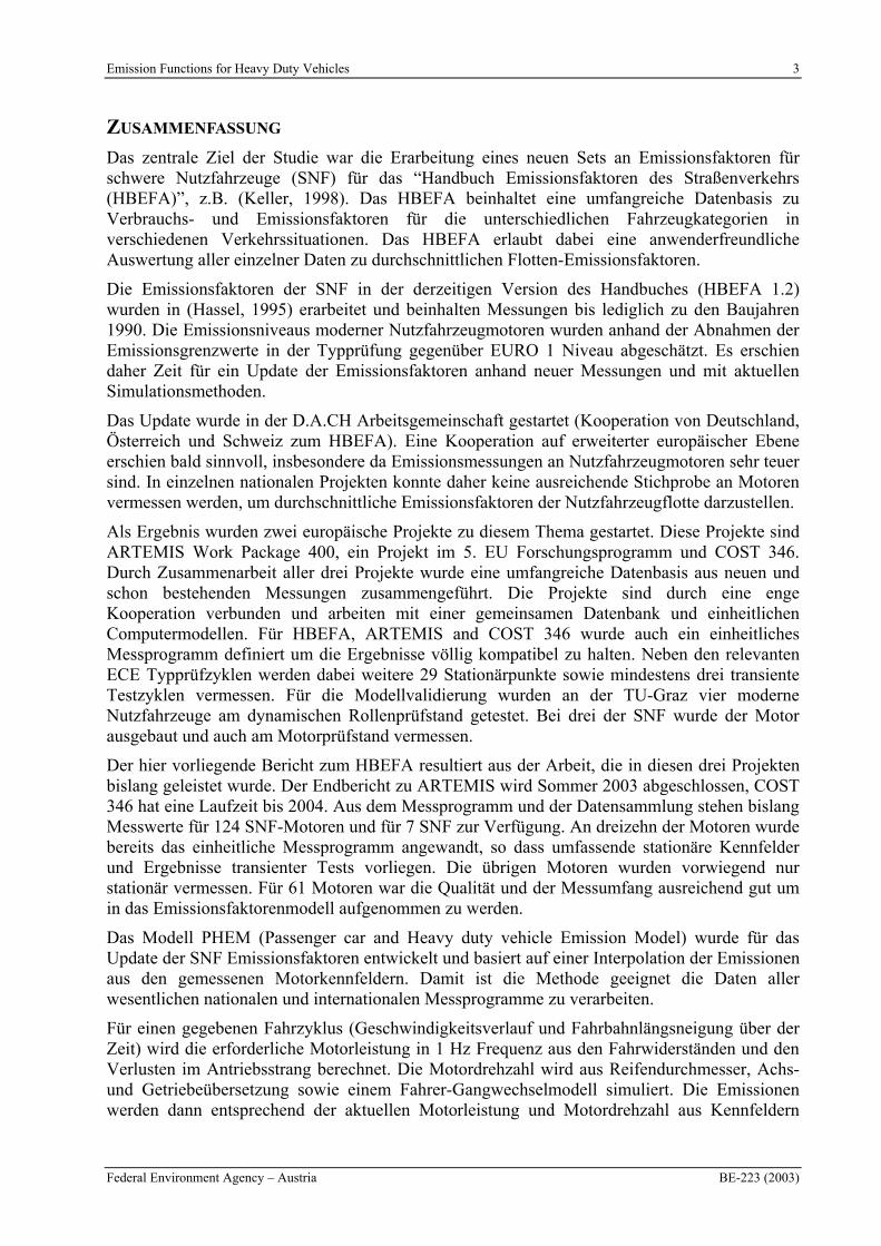
Ein wesentliches Instrument um eine hohe Modellgenauigkeit zu erreichen ist die hier entwickelte Methode der Dynamikkorrektur. Diese Methode transformiert das Emissionsniveau der Emissionskennfelder, die ja stationär gemessen sind, auf das Niveau, das in den jeweiligen transienten Fahrabschnitten zu erwarten ist (Abbildung E1). Das Modell PHEM zeigte sich insgesamt als geeignet alle Bedürfnisse des HBEFA zur Simulation unterschiedlichster Kombinationen von SNF-Kategorien, Beladungen, Fahrzyklen und Fahrbahnlängsneigungen zu erfüllen.
Motorlast, Verbrauch, Emissionen
Motorkennfeld
Fahrwiderstände & ÜbertragungsverlusteFahrwiderstände &
Übertragungsverluste
Gang-wahl-modell
DynamikkorrekturDynamikkorrektur
KaltstartmodulKaltstartmodul
0.00.2
0.40.6
0.81.0
n_norm
-0.20.0
0.20.4
0.60.8
1.0
Pe/P_rated
50
100
150
200
250
FC
0
100
200
300
400
500
600
700
800
900
1000
0 10 20 30 40 50 60 70 80 90
Mittlere Zyklusgeschwindigkeit [km/h]
[g/k
m]
PRE EURO 1EURO 1EURO 2EURO 3EURO 4EURO 5
Verbrauch
Abbildung E1: Schema des Modells PHEM (links) und simulierte Verbrauchswerte für die SNF-Kategorie “Lastenzüge und Sattel-KFZ 34-40t”, halb beladen, 0% Fahrbahnlängsneigung
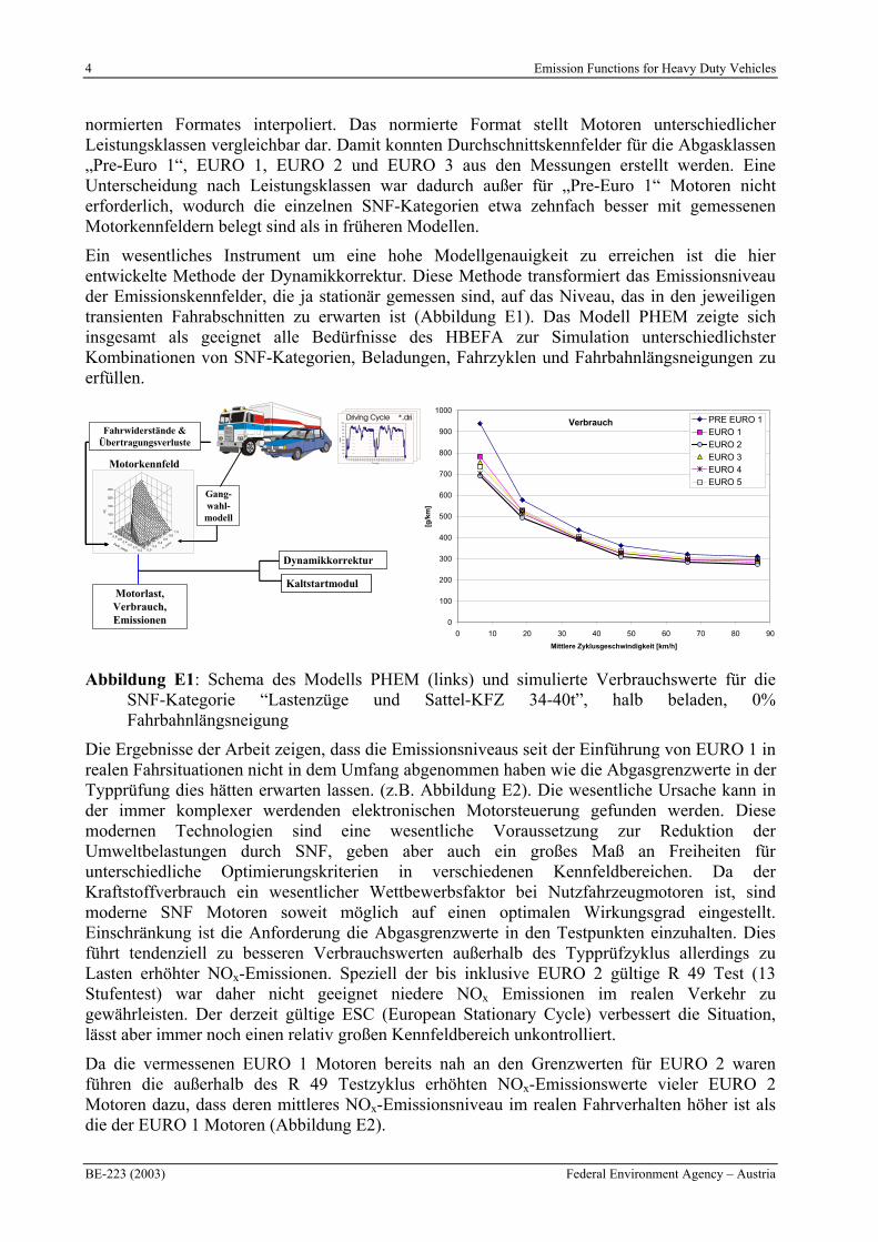
Die Ergebnisse der Arbeit zeigen, dass die Emissionsniveaus seit der Einführung von EURO 1 in realen Fahrsituationen nicht in dem Umfang abgenommen haben wie die Abgasgrenzwerte in der Typprüfung dies hätten erwarten lassen. (z.B. Abbildung E2). Die wesentliche Ursache kann in der immer komplexer werdenden elektronischen Motorsteuerung gefunden werden. Diese modernen Technologien sind eine wesentliche Voraussetzung zur Reduktion der Umweltbelastungen durch SNF, geben aber auch ein großes Maß an Freiheiten für unterschiedliche Optimierungskriterien in verschiedenen Kennfeldbereichen. Da der Kraftstoffverbrauch ein wesentlicher Wettbewerbsfaktor bei Nutzfahrzeugmotoren ist, sind moderne SNF Motoren soweit möglich auf einen optimalen Wirkungsgrad eingestellt. Einschränkung ist die Anforderung die Abgasgrenzwerte in den Testpunkten einzuhalten. Dies führt tendenziell zu besseren Verbrauchswerten außerhalb des Typprüfzyklus allerdings zu Lasten erhöhter NOx-Emissionen. Speziell der bis inklusive EURO 2 gültige R 49 Test (13 Stufentest) war daher nicht geeignet niedere NOx Emissionen im realen Verkehr zu gewährleisten. Der derzeit gültige ESC (European Stationary Cycle) verbessert die Situation, lässt aber immer noch einen relativ großen Kennfeldbereich unkontrolliert.
Da die vermessenen EURO 1 Motoren bereits nah an den Grenzwerten für EURO 2 waren führen die außerhalb des R 49 Testzyklus erhöhten NOx-Emissionswerte vieler EURO 2 Motoren dazu, dass deren mittleres NOx-Emissionsniveau im realen Fahrverhalten höher ist als die der EURO 1 Motoren (Abbildung E2).
Emission Functions for Heavy Duty Vehicles 5
Federal Environment Agency – Austria BE-223 (2003)
Bei Partikelemissionen wurden deutliche Reduktionen von „pre EURO 1“ zu EURO 1 und von EURO 1 zu EURO 2 erreicht. Die EURO 3 Motoren liegen dagegen durchwegs sehr knapp am Grenzwert und haben daher ein ähnliches Partikel-Emissionsniveau wie EURO 2 Motoren obwohl der Grenzwert für EURO 3 um 33% niedriger als für EURO 2 liegt. Allerdings wurden bislang erst vier EURO 3 Motoren gemessen, die auch alle der ersten EURO 3 Generation angehören, so dass hier noch keine sicheren Schlüsse gezogen werden können.
Für die zukünftigen Technologien (EURO 4 and EURO 5 Motoren) ist der ETC (European Transient Cycle) bei der Typprüfung vorgeschrieben. Das sollte die Übereinstimmung der Emissionswerte im realen Verkehr mit den Werten aus der Typprüfung weiter verbessern. Für die Berechnung der Emissionsfaktoren wurde angenommen, dass die EURO 4 und EURO 5 Motoren vorwiegend in dem Kennfeldbereich gefahren werden der auch durch den ETC abgedeckt wird. Ob dies ohne zusätzliche Vorschriften auch allgemein eingehalten werden wird sollte in Zukunft überprüft werden, da die im ETC getesteten Motordrehzahlen von der Vollastkurve der Motoren abhängen, die mit modernen Technologien relativ flexibel gestaltet werden kann. Bei Abweichungen zwischen den im ETC und auf der Strasse gefahrenen Drehzahlen wären eventuell Vorschriften über die zulässigen Achs- und Getriebeübersetzungen der SNF bezogen auf den ETC zu setzen.
0
0.1
0.2
0.3
0.4
0.5
0.6
0.7
0 1 2 3 4 5 6 7
[g/k
Wh
]
PM - Grenzwert
PM - Typprüfung
PM - Autobahn
"Pre EURO" EURO 1 EURO 2 EURO 3 EURO 4 EURO 5 1992 ab 1996 ab 2001 ab 2005 ab 2008
Zukunft ?
0
2
4
6
8
10
12
0 1 2 3 4 5 6 7
NO
x [g
/kW
h]
NOx - Grenzwert
NOx - Typprüfung
NOx - Autobahn
"Pre EURO" EURO 1 EURO 2 EURO 3 EURO 4 EURO 5 1992 ab 1996 ab 2001 ab 2005 ab 2008
Zukunft ?
Abbildung E2: Entwicklung der Emissionsgrenzwerte, der Emissionsniveaus in den zugehörigen Typprüfzyklen und den für realen Autobahnverkehr berechneten Emissionen
Insgesamt wurden mit dem Modell PHEM über 30.000 Emissionsfaktoren für die Kombinationen aus SNF-Kategorien, Fahrzyklen, Fahrzeugbeladungen und Fahrbahnlängsneigungen berechnet. Infolge der sehr unterschiedlichen Applikationsstrategien für EURO 1, EURO 2 und EURO 3 Motoren ergeben sich für verschiedene Fahrzyklen, Beladungen und Steigungen auch sehr unterschiedliche Verhältnisse der Emissionsniveaus zwischen den EURO-Kategorien und noch größere Differenzen zwischen den Motortypen der einzelnen Hersteller. Daher hängt das Verhältnis der Emissionsfaktoren zwischen den einzelnen EURO-Kategorien stark vom Fahrzustand und der Fahrzeugbeladung ab. Als mittlerer Trend nahmen die Verbrauchsfaktoren [g/km] von EURO 1 nach EURO 2 um etwa 15% ab. Die strengeren NOx-Grenzwerte und der breitere kontrollierte Drehzahlbereich im Typprüftest (ESC) für EURO 3 führte zu einem Verbrauchsanstieg von etwa 6% gegenüber EURO 2. Als Beispiel zeigt Abbildung E1 die berechneten Verbrauchswerte für eine SNF-Kategorie auf ebener Fahrbahn mit 50% Beladung.
Die NOx-Emissionen der EURO 2 SNF sind etwa 10% höher als von EURO 1. Fahrzeuge nach EURO 3 zeigen wieder ein geringeres Emissionsniveau, die Verhältnisse hängen aber insbesondere bei EURO 3 stark vom betrachteten Fahrzustand ab (Abbildung E3). Während im schnellen Autobahnverkehr EURO 3 SNF etwa 30% geringere NOx-Emissionen zeigt als
6 Emission Functions for Heavy Duty Vehicles
BE-223 (2003) Federal Environment Agency – Austria
EURO 2, verringert sich dieser Vorteil im langsamen Stop&Go Verkehr auf etwa 5%. Dies ist vorwiegend auf unterschiedliche Motordrehzahlen in den verschiedenen Fahrzyklen zurückzuführen. Bei langsamen Zyklen mit häufigen Anfahrvorgängen werden relativ häufig Drehzahlbereiche angefahren, die vom ESC nicht erfasst werden. Diese Kennfeldbereiche zeigen auch bei EURO 3 Motoren meist Optimierungen der Verbrauchswerte mit entsprechend hohen Stickoxidemissionen. Für EURO 4 werden etwa 30%, für EURO 5 mehr als 60% niedrigere NOx-Emissionsfaktoren gegenüber EURO 3 erwartet. Ein Problem der mit Sicherheit deutlich komplexeren zukünftigen Motortechnologien könnte deren Dauerhaltbarkeit sein. Während Dieselmotoren bislang keine signifikanten Änderungen des Emissionsniveaus über ihrer Lebenszeit zeigte, könnte sich dies in Zukunft ändern.
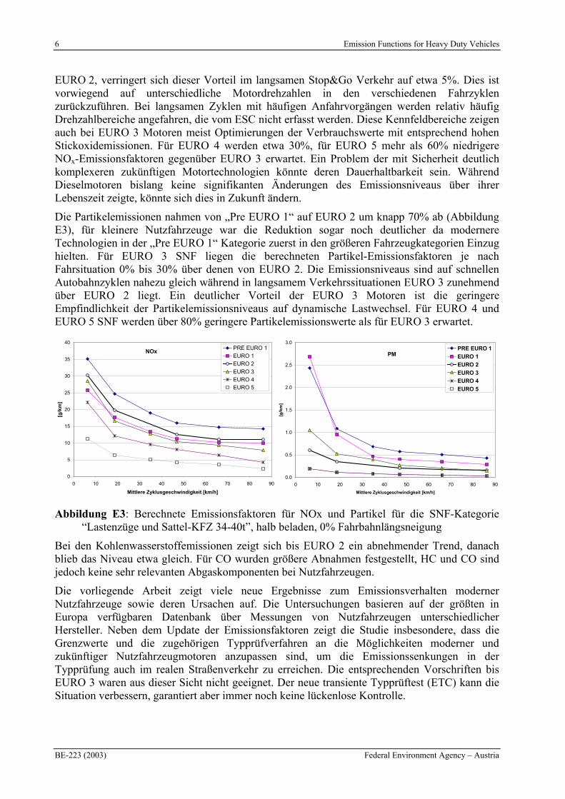
Die Partikelemissionen nahmen von „Pre EURO 1“ auf EURO 2 um knapp 70% ab (Abbildung E3), für kleinere Nutzfahrzeuge war die Reduktion sogar noch deutlicher da modernere Technologien in der „Pre EURO 1“ Kategorie zuerst in den größeren Fahrzeugkategorien Einzug hielten. Für EURO 3 SNF liegen die berechneten Partikel-Emissionsfaktoren je nach Fahrsituation 0% bis 30% über denen von EURO 2. Die Emissionsniveaus sind auf schnellen Autobahnzyklen nahezu gleich während in langsamem Verkehrssituationen EURO 3 zunehmend über EURO 2 liegt. Ein deutlicher Vorteil der EURO 3 Motoren ist die geringere Empfindlichkeit der Partikelemissionsniveaus auf dynamische Lastwechsel. Für EURO 4 und EURO 5 SNF werden über 80% geringere Partikelemissionswerte als für EURO 3 erwartet.
0
5
10
15
20
25
30
35
40
0 10 20 30 40 50 60 70 80 90
Mittlere Zyklusgeschwindigkeit [km/h]
[g/k
m]
PRE EURO 1EURO 1EURO 2EURO 3EURO 4EURO 5
NOx
0.0
0.5
1.0
1.5
2.0
2.5
3.0
0 10 20 30 40 50 60 70 80 90
Mittlere Zyklusgeschwindigkeit [km/h]
[g/k
m]
PRE EURO 1
EURO 1
EURO 2
EURO 3
EURO 4
EURO 5
PM
Abbildung E3: Berechnete Emissionsfaktoren für NOx und Partikel für die SNF-Kategorie “Lastenzüge und Sattel-KFZ 34-40t”, halb beladen, 0% Fahrbahnlängsneigung
Bei den Kohlenwasserstoffemissionen zeigt sich bis EURO 2 ein abnehmender Trend, danach blieb das Niveau etwa gleich. Für CO wurden größere Abnahmen festgestellt, HC und CO sind jedoch keine sehr relevanten Abgaskomponenten bei Nutzfahrzeugen.
Die vorliegende Arbeit zeigt viele neue Ergebnisse zum Emissionsverhalten moderner Nutzfahrzeuge sowie deren Ursachen auf. Die Untersuchungen basieren auf der größten in Europa verfügbaren Datenbank über Messungen von Nutzfahrzeugen unterschiedlicher Hersteller. Neben dem Update der Emissionsfaktoren zeigt die Studie insbesondere, dass die Grenzwerte und die zugehörigen Typprüfverfahren an die Möglichkeiten moderner und zukünftiger Nutzfahrzeugmotoren anzupassen sind, um die Emissionssenkungen in der Typprüfung auch im realen Straßenverkehr zu erreichen. Die entsprechenden Vorschriften bis EURO 3 waren aus dieser Sicht nicht geeignet. Der neue transiente Typprüftest (ETC) kann die Situation verbessern, garantiert aber immer noch keine lückenlose Kontrolle.
Emission Functions for Heavy Duty Vehicles 7
Federal Environment Agency – Austria BE-223 (2003)
1 EXECUTIVE SUMMARY
Main task of the study was the elaboration of a new set of emission factors for Heavy Duty Vehicles (HDV) in the “Handbook on Emission Factors for Road Traffic (HBEFA)”, e.g. (Keller, 1998). The HBEFA contains an extensive data base on fuel consumption values and emission factors for different vehicle categories under different traffic situations and allows a user-friendly aggregation of all the single emission values to average fleet emission factors.
The HDV emission factors implemented in the actual version of the Handbook (HBEFA 1.2) were elaborated in (Hassel, 1995) and include measurements on engines with construction years up to 1990 only. Emission levels for modern engines were estimated according to the limit values in the type approval tests based on measurements at some EURO 1 engines. Thus it seemed to be high time to update the emission factors.
The update was started in the D.A.CH group (cooperation with Germany, Austria and Switzerland on the HBEFA) in 1999, ordered by Austria. A European cooperation on this topic proved to be very sensible, especially since measurements on HDV engines are very expensive. Thus, in single national projects a sufficient number of engines could not be measured to assess the average emission behaviour of HDV on the road. As a result two European projects – dealing with the same topic – were started, both lead by TU-Graz. These projects are ARTEMIS-Work Package 400 (within the 5th framework programme of the EU) and COST 346. Within these projects a broad data base from new measurements and already existing data has been elaborated. All project partners agreed that the HBEFA can use the data and results of the European projects and that at the same time the results and computer programme elaborated for the update of the HBEFA can be used in the European projects. The actual report, thus, is a summary of the work performed in all three projects so far.
HBEFA, ARTEMIS and COST 346 use the same measurement programme including all relevant ECE type approval tests, a 29steady-state point engine emission map and at least three different transient test cycles. For the model, validation measurements of four HDV on the chassis dynamometer of the TU-Graz were performed, for three of them the engine was measured on the engine test bed as well.
From the measurement programme and the data collection emission measurements for 124 HDV engines and for 7 HDV are available. Thirteen of the engine tests include extensive steady state tests and different transient test cycles. For the other engines only steady state measurements were performed. The data of 61 of the engines measured finally approved to be of sufficient quality and were included in the model.
The model PHEM (Passenger car and Heavy duty vehicle Emission model) developed for the update of the HDV emission factors is based on interpolations from the measured engine emission maps. The method is therefore capable of making use of the data from most national and international measurement programmes.
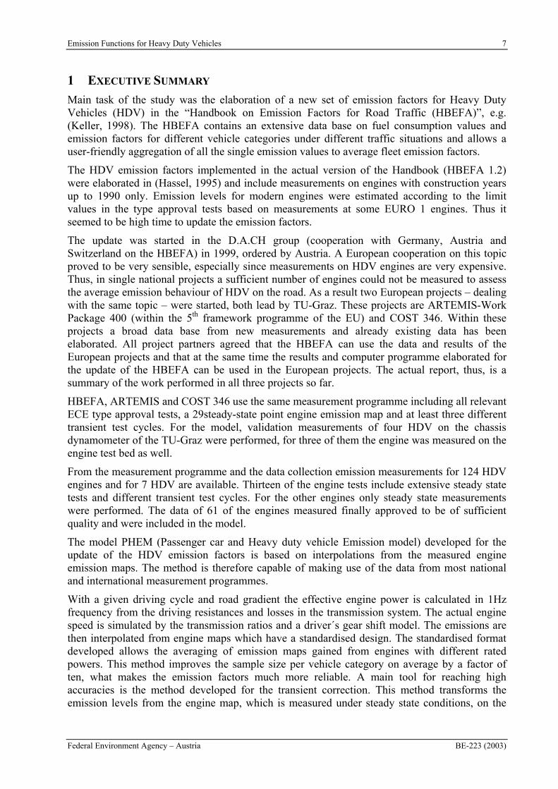
With a given driving cycle and road gradient the effective engine power is calculated in 1Hz frequency from the driving resistances and losses in the transmission system. The actual engine speed is simulated by the transmission ratios and a driver´s gear shift model. The emissions are then interpolated from engine maps which have a standardised design. The standardised format developed allows the averaging of emission maps gained from engines with different rated powers. This method improves the sample size per vehicle category on average by a factor of ten, what makes the emission factors much more reliable. A main tool for reaching high accuracies is the method developed for the transient correction. This method transforms the emission levels from the engine map, which is measured under steady state conditions, on the
8 Emission Functions for Heavy Duty Vehicles
BE-223 (2003) Federal Environment Agency – Austria
emission levels which have to be expected under the actual transient engine load (Figure E1). The model PHEM also proved to be capable of handling the requests from the HBEFA on the simulation of emission factors for traffic situations where no measured driving cycles were available.
Engine load, fuel consumption, emissions
Engine map
Driving resistancese & transmission losses
Gear-shift
model
Transient Correction
Cold Start ToolCold Start Tool
0.00.2
0.40.6
0.81.0
n_norm
-0.20.0
0.20.4
0.60.8
1.0
Pe/P_rated
50
100
150
200
250
FC
0
100
200
300
400
500
600
700
800
900
1000
0 10 20 30 40 50 60 70 80 90
Average cycle speed [km/h]
[g/k
m]
PRE EURO 1EURO 1EURO 2EURO 3EURO 4EURO 5
Fuel consumption
Figure E1: Schema of the model PHEM (left) and simulated fuel consumption values for the HDV-category “semi trailers 34-40t”, half loaded, 0% road gradient
The results of the study show that since the introduction of the EURO 1 limits the emission levels have not decreased in real world driving conditions to the same extent as the emission limits for the type approval have been reduced (e.g. Figure E2). Main reasons are found in the more sophisticated technologies for engine control and fuel injection. On the one hand these modern technologies are a prerequisite for reducing the environmental impacts of HDV engines, on the other hand they give freedom for different specific optimizations at different regions of the engine map. Since fuel costs are a main factor for the competitiveness of HDV engines, manufacturers optimize the engines towards high fuel efficiencies wherever possible. That affects especially the NOx emission levels. The steady state tests at the type approval can thus not ensure low emission levels for real world driving conditions. This was mainly found for EURO 2 engines tested with the R 49 steady state cycle while the European Stationary Cycle (ESC) valid for EURO 3 engines improves the situation. But still a broad range of the engine map is not controlled sufficiently.
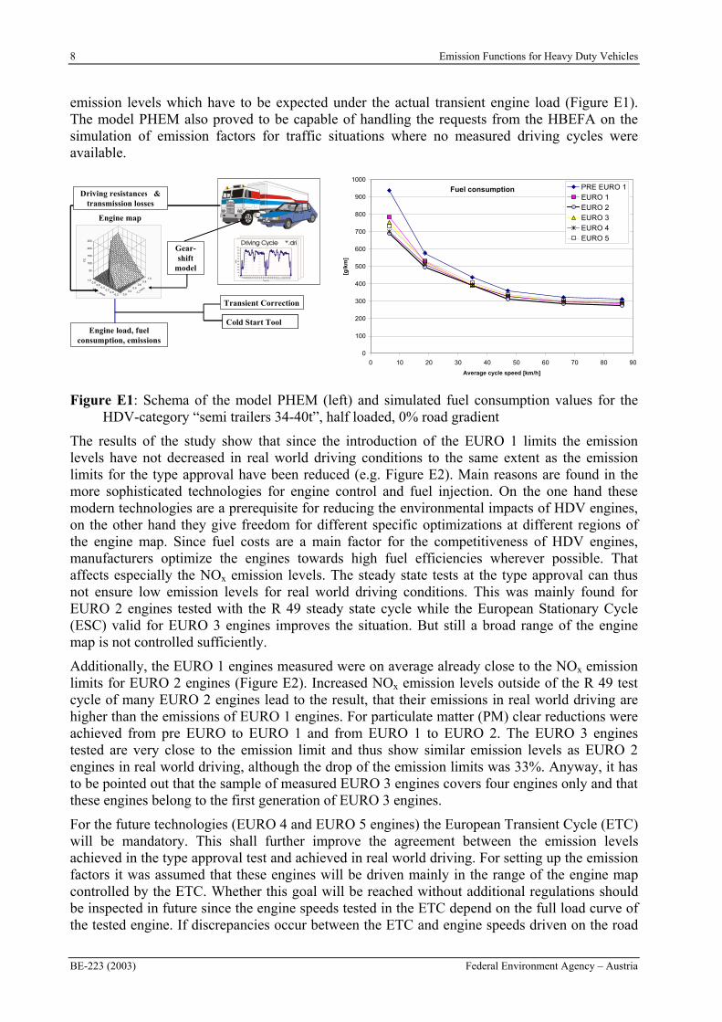
Additionally, the EURO 1 engines measured were on average already close to the NOx emission limits for EURO 2 engines (Figure E2). Increased NOx emission levels outside of the R 49 test cycle of many EURO 2 engines lead to the result, that their emissions in real world driving are higher than the emissions of EURO 1 engines. For particulate matter (PM) clear reductions were achieved from pre EURO to EURO 1 and from EURO 1 to EURO 2. The EURO 3 engines tested are very close to the emission limit and thus show similar emission levels as EURO 2 engines in real world driving, although the drop of the emission limits was 33%. Anyway, it has to be pointed out that the sample of measured EURO 3 engines covers four engines only and that these engines belong to the first generation of EURO 3 engines.
For the future technologies (EURO 4 and EURO 5 engines) the European Transient Cycle (ETC) will be mandatory. This shall further improve the agreement between the emission levels achieved in the type approval test and achieved in real world driving. For setting up the emission factors it was assumed that these engines will be driven mainly in the range of the engine map controlled by the ETC. Whether this goal will be reached without additional regulations should be inspected in future since the engine speeds tested in the ETC depend on the full load curve of the tested engine. If discrepancies occur between the ETC and engine speeds driven on the road
Emission Functions for Heavy Duty Vehicles 9
Federal Environment Agency – Austria BE-223 (2003)
it may be necessary to introduce directions which restrict the transmission ratios of the axis and the gear box from the vehicle according to the engine speeds tested in the ETC.
0
2
4
6
8
10
12
0 1 2 3 4 5 6 7
NO
x [g
/kW
h]
NOx - emission limit
NOx - type approval cycle
NOx - real world highway
"Pre EURO" EURO 1 EURO 2 EURO 3 EURO 4 EURO 5
Assessment
0
0.1
0.2
0.3
0.4
0.5
0.6
0.7
0 1 2 3 4 5 6 7
[g/k
Wh
]
PM - emission limit
PM - type approval cycle
PM - real world highway
"Pre EURO" EURO 1 EURO 2 EURO 3 EURO 4 EURO 5
Assessment
Figure E2: Development of the emission limits, the emission levels measured on average in the corresponding test cycles and the emissions simulated for real world highway driving
In total for more than 30.000 combinations of vehicle categories, EURO-categories, driving cycles, vehicle loadings and road gradients emission factors were simulated with the model PHEM. Due to the different strategies for the application work at the engines for EURO 1, EURO 2 and EURO 3 the emission behavior of the HDV under different vehicle loads, driving cycles and road gradient is very different for the different EURO classes and much more different for the single makes and models of engines.
As a result, the ratios of the emission factors between the EURO categories pre EURO 1 to EURO 3 depend on the driving cycle, the road gradient and the vehicle loadings. As a general trend of the measurements and the simulation of the emission factors fuel consumption values proved to drop from “pre EURO 1” to EURO 2 by approximately 15%. The more stringent NOx
limits and the broader controlled engine speed range of the ESC test for EURO 3 lead to an increase in the fuel consumption in the range of 6% from EURO 2 to EURO 3. As an example figure E1 gives the results for one HDV category with 50% loading on a flat road.
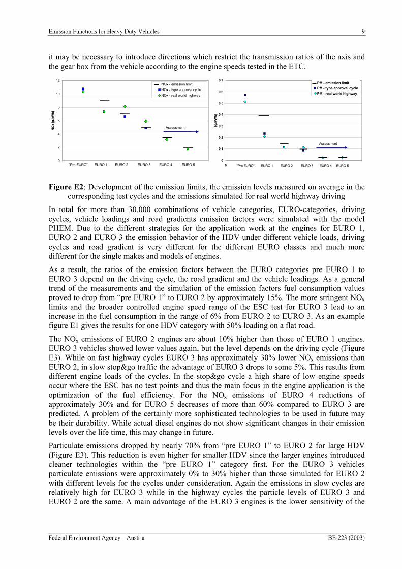
The NOx emissions of EURO 2 engines are about 10% higher than those of EURO 1 engines. EURO 3 vehicles showed lower values again, but the level depends on the driving cycle (Figure E3). While on fast highway cycles EURO 3 has approximately 30% lower NOx emissions than EURO 2, in slow stop&go traffic the advantage of EURO 3 drops to some 5%. This results from different engine loads of the cycles. In the stop&go cycle a high share of low engine speeds occur where the ESC has no test points and thus the main focus in the engine application is the optimization of the fuel efficiency. For the NOx emissions of EURO 4 reductions of approximately 30% and for EURO 5 decreases of more than 60% compared to EURO 3 are predicted. A problem of the certainly more sophisticated technologies to be used in future may be their durability. While actual diesel engines do not show significant changes in their emission levels over the life time, this may change in future.
Particulate emissions dropped by nearly 70% from “pre EURO 1” to EURO 2 for large HDV (Figure E3). This reduction is even higher for smaller HDV since the larger engines introduced cleaner technologies within the “pre EURO 1” category first. For the EURO 3 vehicles particulate emissions were approximately 0% to 30% higher than those simulated for EURO 2 with different levels for the cycles under consideration. Again the emissions in slow cycles are relatively high for EURO 3 while in the highway cycles the particle levels of EURO 3 and EURO 2 are the same. A main advantage of the EURO 3 engines is the lower sensitivity of the
10 Emission Functions for Heavy Duty Vehicles
BE-223 (2003) Federal Environment Agency – Austria
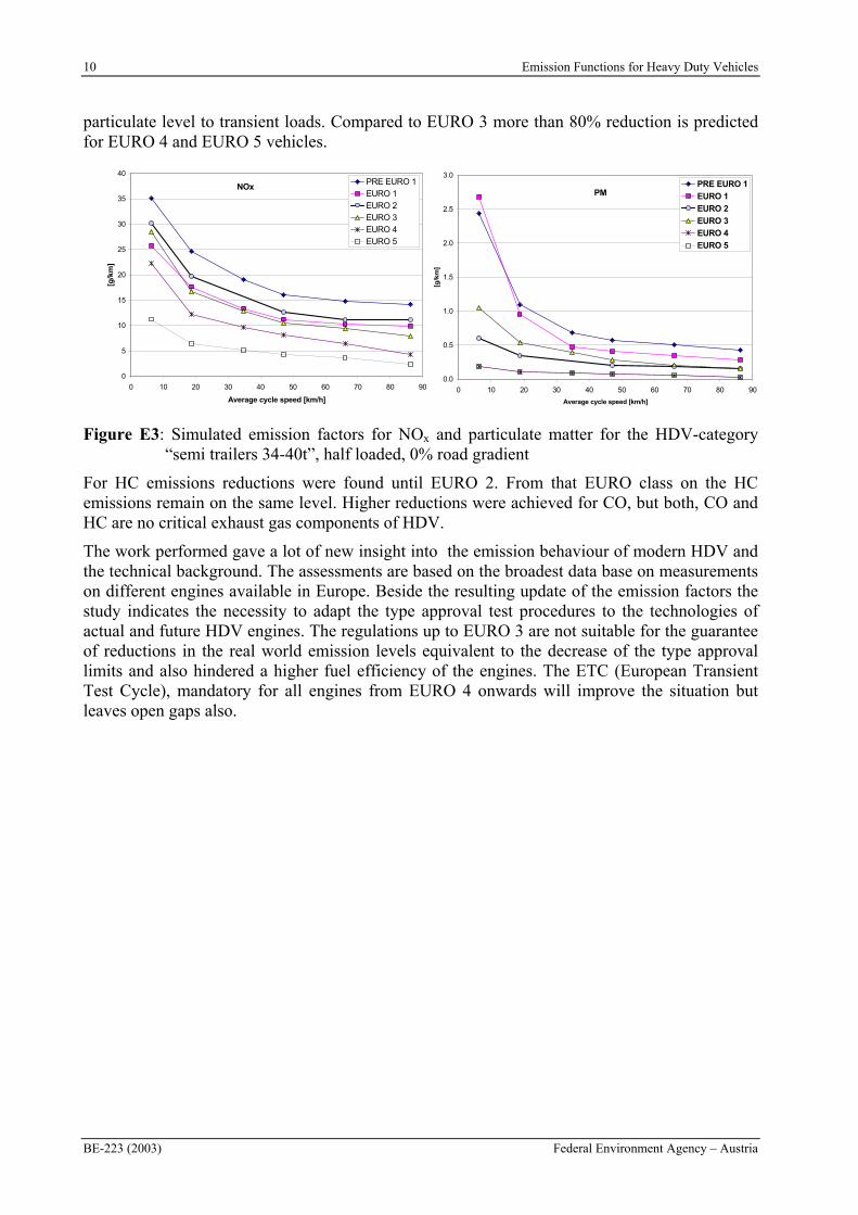
particulate level to transient loads. Compared to EURO 3 more than 80% reduction is predicted for EURO 4 and EURO 5 vehicles.
0
5
10
15
20
25
30
35
40
0 10 20 30 40 50 60 70 80 90
Average cycle speed [km/h]
[g/k
m]
PRE EURO 1EURO 1EURO 2EURO 3EURO 4EURO 5
NOx
0.0
0.5
1.0
1.5
2.0
2.5
3.0
0 10 20 30 40 50 60 70 80 90
Average cycle speed [km/h]
[g/k
m]
PRE EURO 1
EURO 1
EURO 2
EURO 3
EURO 4
EURO 5
PM
Figure E3: Simulated emission factors for NOx and particulate matter for the HDV-category “semi trailers 34-40t”, half loaded, 0% road gradient
For HC emissions reductions were found until EURO 2. From that EURO class on the HC emissions remain on the same level. Higher reductions were achieved for CO, but both, CO and HC are no critical exhaust gas components of HDV.
The work performed gave a lot of new insight into the emission behaviour of modern HDV and the technical background. The assessments are based on the broadest data base on measurements on different engines available in Europe. Beside the resulting update of the emission factors the study indicates the necessity to adapt the type approval test procedures to the technologies of actual and future HDV engines. The regulations up to EURO 3 are not suitable for the guarantee of reductions in the real world emission levels equivalent to the decrease of the type approval limits and also hindered a higher fuel efficiency of the engines. The ETC (European Transient Test Cycle), mandatory for all engines from EURO 4 onwards will improve the situation but leaves open gaps also.
Emission Functions for Heavy Duty Vehicles 11
Federal Environment Agency – Austria BE-223 (2003)
2 INTRODUCTION
In a German, an Austrian and a Swiss cooperation (D.A.CH.) the “Handbook of Emission Factors for Road Traffic” was established in the 90s. While emission functions for Light Duty Vehicles (LDV) have been updated with measurements regularly, the Heavy Duty Vehicle (HDV) emission values still were based on measurements of engines constructed between 1984 and 1990 (Hassel, 1995).
Scope of the work was to update the emission functions for HDV with measurements of new HDV and HDV engines and to improve the general methodology for the elaboration of emission functions for HDV.
In the original planning it was intended to measure 3 modern HDV on the chassis dynamometer and to measure their engines on the engine test bed too. In the meantime two European projects – dealing with the same topic – were started, both lead by the TU-Graz. These projects are ARTEMIS-Work Package 400 (within the 5th framework programme of the EU) and COST 346. Within these projects a broad data base on new measurements and already existing data has been elaborated. All project partners agreed that the work for D.A.CH can use the data and results from the European projects and that on the other hand the results and computer programme elaborated for the D.A.CH project can be used in the European projects.
Thus data on more than 120 different engines was available for the D.A.CH. project, 13 of these engines were measured according to a detailed common protocol, which was elaborated for the D.A.CH project first and was then introduced for the European projects in a revised version. These measurements include a 54 steady state point engine emission map and the test of at least three different transient cycles. Measurements of four HDV on the chassis dynamometer of the TU-Graz were used for the model validation, for three of them the engine was measured on the engine test bed too.
For the simulation of the HDV emission factors a detailed simulation program was developed. The model PHEM (Passenger car and Heavy duty Emission model) is capable of calculating fuel consumption and emissions for any vehicles and driving cycles with a high accuracy using engine emission maps and transient correction functions.
3 APPROACH
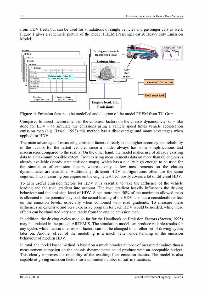
The targeted results are emission factors for different categories of the HDV fleet (separated according to engine technology and vehicle weight classes) with different loadings of the HDV for different representative driving cycles at different road gradients (Figure 1). The results are emission factors for more than 30.000 combinations of vehicle categories, driving cycles, road gradients and vehicle loadings. These emission factors are then used as an input for the “Handbook Emission Factors” e.g. (Keller,1998), which is a databank that allows the user a simple simulation of aggregated emission factors for different traffic situations.
For the elaboration of the emission factors a methodology based on interpolations from steady state emission maps was chosen, since data on more than 100 measurements of engine maps are already available which should be used in the model. With a given driving cycle and road gradient the necessary engine power is calculated second per second from the driving resistances and losses in the transmission system. The actual engine speed is simulated by the transmission ratios and a driver´s gear-shift model. To take transient influences on the emission level into consideration, the results from the steady state emission map are corrected by using transient correction functions. The method was implemented into a computer executable model with a user-friendly interface. The model is optimised for simulating fuel consumption and emissions
12 Emission Functions for Heavy Duty Vehicles
BE-223 (2003) Federal Environment Agency – Austria
from HDV fleets but can be used for simulations of single vehicles and passenger cars as well. Figure 1 gives a schematic picture of the model PHEM (Passenger car & Heavy duty Emission Model).
cycle 1 cycle 2 cycle 3 cycle 4 cycle 5 ..... ....truck <7,5ttruck 7,5-14ttruck 14-20ttruck 20-28ttruck trailer <20ttruck trailer20-28ttruck trailer 28-32ttruck trailer>32tsemi trailer<32tsemi trailer >32tcity bus <8t.........
EURO 5cycle 1 cycle 2 cycle 3 cycle 4 cycle 5 ..... ....
truck <7,5ttruck 7,5-14ttruck 14-20ttruck 20-28ttruck trailer <20ttruck trailer20-28ttruck trailer 28-32ttruck trailer>32tsemi trailer<32tsemi trailer >32tcity bus <8t.........
EURO 5
cycle 1 cycle 2 cycle 3 cycle 4 cycle 5 ..... ....truck <7,5ttruck 7,5-14ttruck 14-20ttruck 20-28ttruck trailer <20ttruck trailer20-28ttruck trailer 28-32ttruck trailer>32tsemi trailer<32tsemi trailer >32tcity bus <8t.........
EURO 4cycle 1 cycle 2 cycle 3 cycle 4 cycle 5 ..... ....
truck <7,5ttruck 7,5-14ttruck 14-20ttruck 20-28ttruck trailer <20ttruck trailer20-28ttruck trailer 28-32ttruck trailer>32tsemi trailer<32tsemi trailer >32tcity bus <8t.........
EURO 4
cycle 1 cycle 2 cycle 3 cycle 4 cycle 5 ..... ....truck <7,5ttruck 7,5-14ttruck 14-20ttruck 20-28ttruck trailer <20ttruck trailer20-28ttruck trailer 28-32ttruck trailer>32tsemi trailer<32tsemi trailer >32tcity bus <8t.........
EURO 3cycle 1 cycle 2 cycle 3 cycle 4 cycle 5 ..... ....
truck <7,5ttruck 7,5-14ttruck 14-20ttruck 20-28ttruck trailer <20ttruck trailer20-28ttruck trailer 28-32ttruck trailer>32tsemi trailer<32tsemi trailer >32tcity bus <8t.........
EURO 3
cycle 1 cycle 2 cycle 3 cycle 4 cycle 5 ..... ....truck <7,5ttruck 7,5-14ttruck 14-20ttruck 20-28ttruck trailer <20ttruck trailer20-28ttruck trailer 28-32ttruck trailer>32tsemi trailer<32tsemi trailer >32tcity bus <8t.........
EURO 2cycle 1 cycle 2 cycle 3 cycle 4 cycle 5 ..... ....
truck <7,5ttruck 7,5-14ttruck 14-20ttruck 20-28ttruck trailer <20ttruck trailer20-28ttruck trailer 28-32ttruck trailer>32tsemi trailer<32tsemi trailer >32tcity bus <8t.........
EURO 2
cycle 1 cycle 2 cycle 3 cycle 4 cycle 5 ..... ....truck <7,5ttruck 7,5-14ttruck 14-20ttruck 20-28ttruck trailer <20ttruck trailer20-28ttruck trailer 28-32ttruck trailer>32tsemi trailer<32tsemi trailer >32tcity bus <8t.........
EURO 1cycle 1 cycle 2 cycle 3 cycle 4 cycle 5 ..... ....
truck <7,5ttruck 7,5-14ttruck 14-20ttruck 20-28ttruck trailer <20ttruck trailer20-28ttruck trailer 28-32ttruck trailer>32tsemi trailer<32tsemi trailer >32tcity bus <8t.........
EURO 1
cycle 1 cycle 2 cycle 3 cycle 4 cycle 5 ..... ....truck <7,5ttruck 7,5-14ttruck 14-20ttruck 20-28ttruck trailer <20ttruck trailer20-28ttruck trailer 28-32ttruck trailer>32tsemi trailer<32tsemi trailer >32tcity bus <8t.........
Pre EURO 1cycle 1 cycle 2 cycle 3 cycle 4 cycle 5 ..... ....
truck <7,5ttruck 7,5-14ttruck 14-20ttruck 20-28ttruck trailer <20ttruck trailer20-28ttruck trailer 28-32ttruck trailer>32tsemi trailer<32tsemi trailer >32tcity bus <8t.........
Pre EURO 1
x 3 loadings(empty, 50%, full)
x 6 road gradients(-6%, -4%.....+6%)
Emission factors [g/km] for:FC, NOx, PM, HC, CO
Engine load, FC, emissions
5001000
15002000
25003000
U/min-200
-1000
100200
300400
500600
700800
900
Nm
20000
40000
60000
80000
100000
120000
140000
CO
2[g
/h]
Emission Map
Driving resistances & transmission losses
Gear shift
model
5001000
15002000
25003000
U/min-200
-1000
100200
300400
500600
700800
900
Nm
20000
40000
60000
80000
100000
120000
140000
CO
2[g
/h]
Emission Map
Driving resistances & transmission losses
Gear shift
model
5001000
15002000
25003000
U/min-200
-1000
100200
300400
500600
700800
900
Nm
20000
40000
60000
80000
100000
120000
140000
CO
2[g
/h]
5001000
15002000
25003000
U/min-200
-1000
100200
300400
500600
700800
900
Nm
20000
40000
60000
80000
100000
120000
140000
CO
2[g
/h]
Emission Map
Driving resistances & transmission losses
Driving resistances & transmission losses
Gear shift
model
Transient CorrectionTransient Correction
Cold start toolCold start tool
Engine load, FC, Emissions
Figure 1: Emission factors to be modelled and diagram of the model PHEM from TU-Graz
Compared to direct measurement of the emission factors on the chassis dynamometer or – like done for LDV – to simulate the emissions using a vehicle speed times vehicle acceleration emission map (e.g. Hassel, 1993) this method has a disadvantage and many advantages when applied for HDV.
The main advantage of measuring emission factors directly is the higher accuracy and reliability of the factors for the tested vehicles since a model always has some simplifications and inaccuracies compared to the reality. On the other hand, the model makes use of already existing data to a maximum possible extent. From existing measurements data on more than 60 engines is already available (steady state emission maps), which has a quality high enough to be used for the simulation of emission factors whereas only a few measurements on the chassis dynamometer are available. Additionally, different HDV configurations often use the same engines. Thus measuring one engine on the engine test bed mostly covers a lot of different HDV.
To gain useful emission factors for HDV it is essential to take the influence of the vehicle loading and the road gradient into account. The road gradient heavily influences the driving behaviour and the emission level of HDV. Since more than 50% of the maximum allowed mass is allocated to the potential payload, the actual loading of the HDV also has a considerable effect on the emission levels, especially when combined with road gradients. To measure these influences an extensive and very expensive program for each HDV would be needed, while these effects can be simulated very accurately from the engine emission map.
In addition, the driving cycles used so far for the Handbook on Emission Factors (Steven, 1995) may be updated in the project ARTEMIS. The simulation model can produce reliable results for any cycles while measured emission factors can not be changed to an other set of driving cycles later on. Another effect of the modelling is a much better understanding of the emission behaviour of modern HDV.
In total, the model based method is based on a much broader number of measured engines than a measurement campaign on the chassis dynamometer could produce with an acceptable budget. This clearly improves the reliability of the resulting fleet emission factors. The model is also capable of giving emission factors for a unlimited number of traffic situations.
Emission Functions for Heavy Duty Vehicles 13
Federal Environment Agency – Austria BE-223 (2003)
4 DATA USED
The D.A.CH.-model makes use of already existing measurements to a large extent. For this purpose a coordinated data collection of all partners from ARTEMIS-WP 400 and COST 346 was launched using standardised formats for data transfer (chapter 13). The measurement programme for the D.A.CH. project and accordingly for ARTEMIS-WP 400 was designed to fill open gaps and to develop a method capable of using all the data in a consistent way. Certainly the data gained from the new measurements are included into the data collection.
From the data collection campaign measurements on 122 engines are available. For approximately half of the engines only emission maps from the 13-mode test (R 49) and the new ESC are available. For the others additional off-cycle points have been measured in the steady state tests. For 15 engines transient tests and complete steady state emission maps are available. Thirteen of these engines have already been measured according to the ARTEMIS measurement programme. Most of the engines measured were derived from HDV in use for two months up to 2 years with regular service intervals.
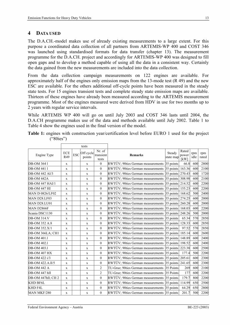
While ARTEMIS WP 400 will go on until July 2003 and COST 346 lasts until 2004, the D.A.CH programme makes use of the data and methods available until July 2002. Table 1 to Table 4 show the engines used in the final version of the model.
Table 1: engines with construction year/certification level before EURO 1 used for the project (“80ies”)
tests
Engine Type ECER49
ESCOff cycle
points
Nr. of transient
testsRemarks
Steady state map
Rated power[kW]
rpmidle
rpmrated
DB-OM 364 l x x 0 RWTÜV; 90ties German measurements 35 points 66.8 600 2800
DB-OM 441 l x x 0 RWTÜV; 90ties German measurements 35 points 163.36 600 2100
DB-OM 442 AI/3 x x 0 RWTÜV; 90ties German measurements 35 points 270.43 600 1720
DB-OM 442A x x 0 RWTÜV; 90ties German measurements 35 points 308.98 600 2100
DB-OM 447 HAI/1 x x 0 RWTÜV; 90ties German measurements 35 points 214.52 600 2200
DB-OM 447 HI x x 0 RWTÜV; 90ties German measurements 35 points 155.23 600 2200
MAN D 0826/LF02 x x 0 RWTÜV; 90ties German measurements 35 points 168.62 500 2400
MAN D28.LF03 x x 0 RWTÜV; 90ties German measurements 35 points 274.25 600 2000
MAN D28.LU01 x x 0 RWTÜV; 90ties German measurements 35 points 260.28 600 2000
MAN D2866F x x 0 RWTÜV; 90ties German measurements 35 points 168.03 600 2200
Scania DSC1130 x x 0 RWTÜV; 90ties German measurements 35 points 248.26 500 2000
DB-OM 314.V x x 0 RWTÜV; 90ties German measurements 35 points 65.34 570 2850
DB-OM 352 A.8 x x 0 RWTÜV; 90ties German measurements 35 points 128.33 600 2850
DB-OM 352.X/1 x x 0 RWTÜV; 90ties German measurements 35 points 97.52 570 2850
DB-OM 366LA; CH1 x x 0 RWTÜV; 90ties German measurements 35 points 185.14 600 2600
DB-OM 401.l x x 0 RWTÜV; 90ties German measurements 35 points 148.89 600 2400
DB-OM 402.l x x 0 RWTÜV; 90ties German measurements 35 points 198.52 600 2400
DB-OM 403.l x x 0 RWTÜV; 90ties German measurements 35 points 223.38 600 2500
DB-OM 407 HX x x 0 RWTÜV; 90ties German measurements 35 points 177.4 500 2200
DB-OM 422 i/3 x x 0 RWTÜV; 90ties German measurements 35 points 205.61 600 2300
DB-OM 422.A.ll/5 x x 0 RWTÜV; 90ties German measurements 35 points 241.65 600 2300
DB-OM 442 A x x 2 TU-Graz; 90ties German measurements 35 Points 269 600 2100
DB-OM 447 hII x x 2 TU-Graz; 90ties German measurements 35 Points 177 600 2200
DB-OM 447hll; CH 2 x x 0 RWTÜV; 90ties German measurements 35 points 179.7 800 2200
KHD BF6L x x 0 RWTÜV; 90ties German measurements 35 points 114.99 650 2500
KHD F4L x x 0 RWTÜV; 90ties German measurements 35 points 64.29 650 2800
MAN MKF/280 x x 0 RWTÜV; 90ties German measurements 35 points 201.7 500 2200
14 Emission Functions for Heavy Duty Vehicles
BE-223 (2003) Federal Environment Agency – Austria
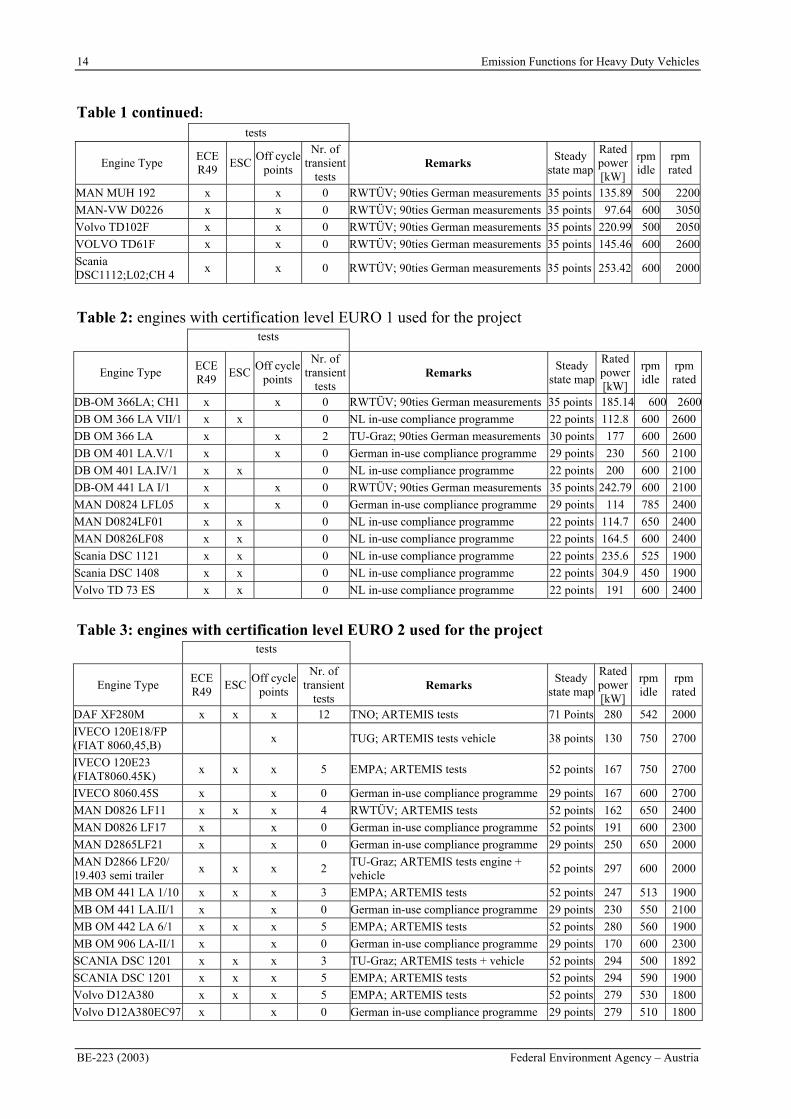
Table 1 continued:
tests
Engine Type ECER49
ESCOff cycle
points
Nr. of transient
testsRemarks
Steady state map
Rated power[kW]
rpmidle
rpmrated
MAN MUH 192 x x 0 RWTÜV; 90ties German measurements 35 points 135.89 500 2200
MAN-VW D0226 x x 0 RWTÜV; 90ties German measurements 35 points 97.64 600 3050
Volvo TD102F x x 0 RWTÜV; 90ties German measurements 35 points 220.99 500 2050
VOLVO TD61F x x 0 RWTÜV; 90ties German measurements 35 points 145.46 600 2600
Scania DSC1112;L02;CH 4
x x 0 RWTÜV; 90ties German measurements 35 points 253.42 600 2000
Table 2: engines with certification level EURO 1 used for the project tests
Engine Type ECER49
ESCOff cycle
points
Nr. of transient
testsRemarks
Steady state map
Rated power[kW]
rpmidle
rpmrated
DB-OM 366LA; CH1 x x 0 RWTÜV; 90ties German measurements 35 points 185.14 600 2600
DB OM 366 LA VII/1 x x 0 NL in-use compliance programme 22 points 112.8 600 2600
DB OM 366 LA x x 2 TU-Graz; 90ties German measurements 30 points 177 600 2600
DB OM 401 LA.V/1 x x 0 German in-use compliance programme 29 points 230 560 2100
DB OM 401 LA.IV/1 x x 0 NL in-use compliance programme 22 points 200 600 2100
DB-OM 441 LA I/1 x x 0 RWTÜV; 90ties German measurements 35 points 242.79 600 2100
MAN D0824 LFL05 x x 0 German in-use compliance programme 29 points 114 785 2400
MAN D0824LF01 x x 0 NL in-use compliance programme 22 points 114.7 650 2400
MAN D0826LF08 x x 0 NL in-use compliance programme 22 points 164.5 600 2400
Scania DSC 1121 x x 0 NL in-use compliance programme 22 points 235.6 525 1900
Scania DSC 1408 x x 0 NL in-use compliance programme 22 points 304.9 450 1900
Volvo TD 73 ES x x 0 NL in-use compliance programme 22 points 191 600 2400
Table 3: engines with certification level EURO 2 used for the project tests
Engine Type ECER49
ESCOff cycle
points
Nr. of transient
testsRemarks
Steady state map
Rated power[kW]
rpmidle
rpmrated
DAF XF280M x x x 12 TNO; ARTEMIS tests 71 Points 280 542 2000
IVECO 120E18/FP (FIAT 8060,45,B)
x TUG; ARTEMIS tests vehicle 38 points 130 750 2700
IVECO 120E23 (FIAT8060.45K)
x x x 5 EMPA; ARTEMIS tests 52 points 167 750 2700
IVECO 8060.45S x x 0 German in-use compliance programme 29 points 167 600 2700
MAN D0826 LF11 x x x 4 RWTÜV; ARTEMIS tests 52 points 162 650 2400
MAN D0826 LF17 x x 0 German in-use compliance programme 52 points 191 600 2300
MAN D2865LF21 x x 0 German in-use compliance programme 29 points 250 650 2000
MAN D2866 LF20/ 19.403 semi trailer
x x x 2 TU-Graz; ARTEMIS tests engine + vehicle
52 points 297 600 2000
MB OM 441 LA 1/10 x x x 3 EMPA; ARTEMIS tests 52 points 247 513 1900
MB OM 441 LA.II/1 x x 0 German in-use compliance programme 29 points 230 550 2100
MB OM 442 LA 6/1 x x x 5 EMPA; ARTEMIS tests 52 points 280 560 1900
MB OM 906 LA-II/1 x x 0 German in-use compliance programme 29 points 170 600 2300
SCANIA DSC 1201 x x x 3 TU-Graz; ARTEMIS tests + vehicle 52 points 294 500 1892
SCANIA DSC 1201 x x x 5 EMPA; ARTEMIS tests 52 points 294 590 1900
Volvo D12A380 x x x 5 EMPA; ARTEMIS tests 52 points 279 530 1800
Volvo D12A380EC97 x x 0 German in-use compliance programme 29 points 279 510 1800
Emission Functions for Heavy Duty Vehicles 15
Federal Environment Agency – Austria BE-223 (2003)
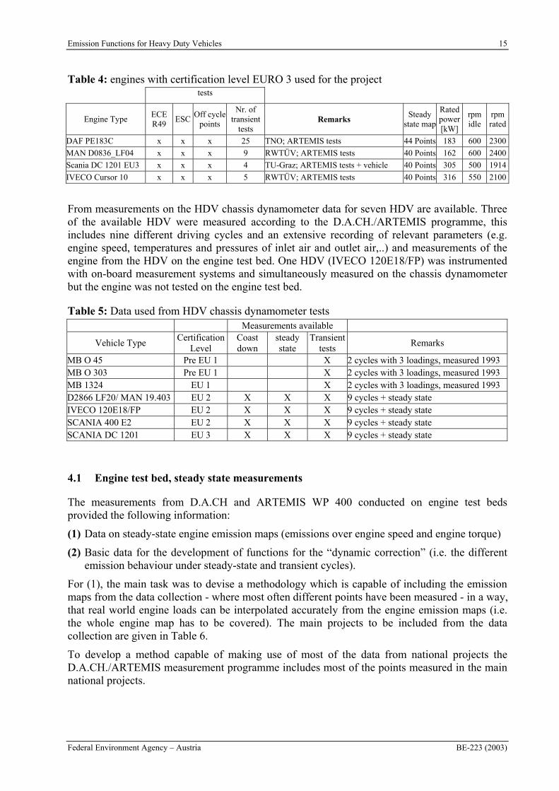
Table 4: engines with certification level EURO 3 used for the project tests
Engine Type ECER49
ESCOff cycle
points
Nr. of transient
testsRemarks
Steady state map
Rated power[kW]
rpmidle
rpmrated
DAF PE183C x x x 25 TNO; ARTEMIS tests 44 Points 183 600 2300
MAN D0836_LF04 x x x 9 RWTÜV; ARTEMIS tests 40 Points 162 600 2400
Scania DC 1201 EU3 x x x 4 TU-Graz; ARTEMIS tests + vehicle 40 Points 305 500 1914
IVECO Cursor 10 x x x 5 RWTÜV; ARTEMIS tests 40 Points 316 550 2100
From measurements on the HDV chassis dynamometer data for seven HDV are available. Three of the available HDV were measured according to the D.A.CH./ARTEMIS programme, this includes nine different driving cycles and an extensive recording of relevant parameters (e.g. engine speed, temperatures and pressures of inlet air and outlet air,..) and measurements of the engine from the HDV on the engine test bed. One HDV (IVECO 120E18/FP) was instrumented with on-board measurement systems and simultaneously measured on the chassis dynamometer but the engine was not tested on the engine test bed.
Table 5: Data used from HDV chassis dynamometer tests Measurements available
Vehicle Type Certification
LevelCoastdown
steadystate
Transienttests
Remarks
MB O 45 Pre EU 1 X 2 cycles with 3 loadings, measured 1993 MB O 303 Pre EU 1 X 2 cycles with 3 loadings, measured 1993 MB 1324 EU 1 X 2 cycles with 3 loadings, measured 1993 D2866 LF20/ MAN 19.403 EU 2 X X X 9 cycles + steady state IVECO 120E18/FP EU 2 X X X 9 cycles + steady state SCANIA 400 E2 EU 2 X X X 9 cycles + steady state SCANIA DC 1201 EU 3 X X X 9 cycles + steady state
4.1 Engine test bed, steady state measurements
The measurements from D.A.CH and ARTEMIS WP 400 conducted on engine test beds provided the following information:
(1) Data on steady-state engine emission maps (emissions over engine speed and engine torque)
(2) Basic data for the development of functions for the “dynamic correction” (i.e. the different emission behaviour under steady-state and transient cycles).
For (1), the main task was to devise a methodology which is capable of including the emission maps from the data collection - where most often different points have been measured - in a way, that real world engine loads can be interpolated accurately from the engine emission maps (i.e. the whole engine map has to be covered). The main projects to be included from the data collection are given in Table 6.
To develop a method capable of making use of most of the data from national projects the D.A.CH./ARTEMIS measurement programme includes most of the points measured in the main national projects.
16 Emission Functions for Heavy Duty Vehicles
BE-223 (2003) Federal Environment Agency – Austria
Table 6: Description of the main national measurement programmes on HDV engines
Programme No. of engines Engine maps available
Netherlands in-use-compliance tests
more than 100 13-mode test, some ESC additionally
German in-use-compliance tests 20 26 different points of engine speed and engine torque
Former German HDV-programme
3035 different points of engine speed and engine torque (all engines older than year 1993)
Smaller national programmes more than 10 13-mode-test, ESC, others
Total: >160 > 4 different map-configurations
The following steady-state measurements are included in the ARTEMIS programme:
R 49 (13-mode test)
ESC (European Steady State Cycle)
ARTEMIS-steady state
The 13-mode test and the ESC have to be performed as given in the corresponding EC documents. This also includes the record of the full-load curve.
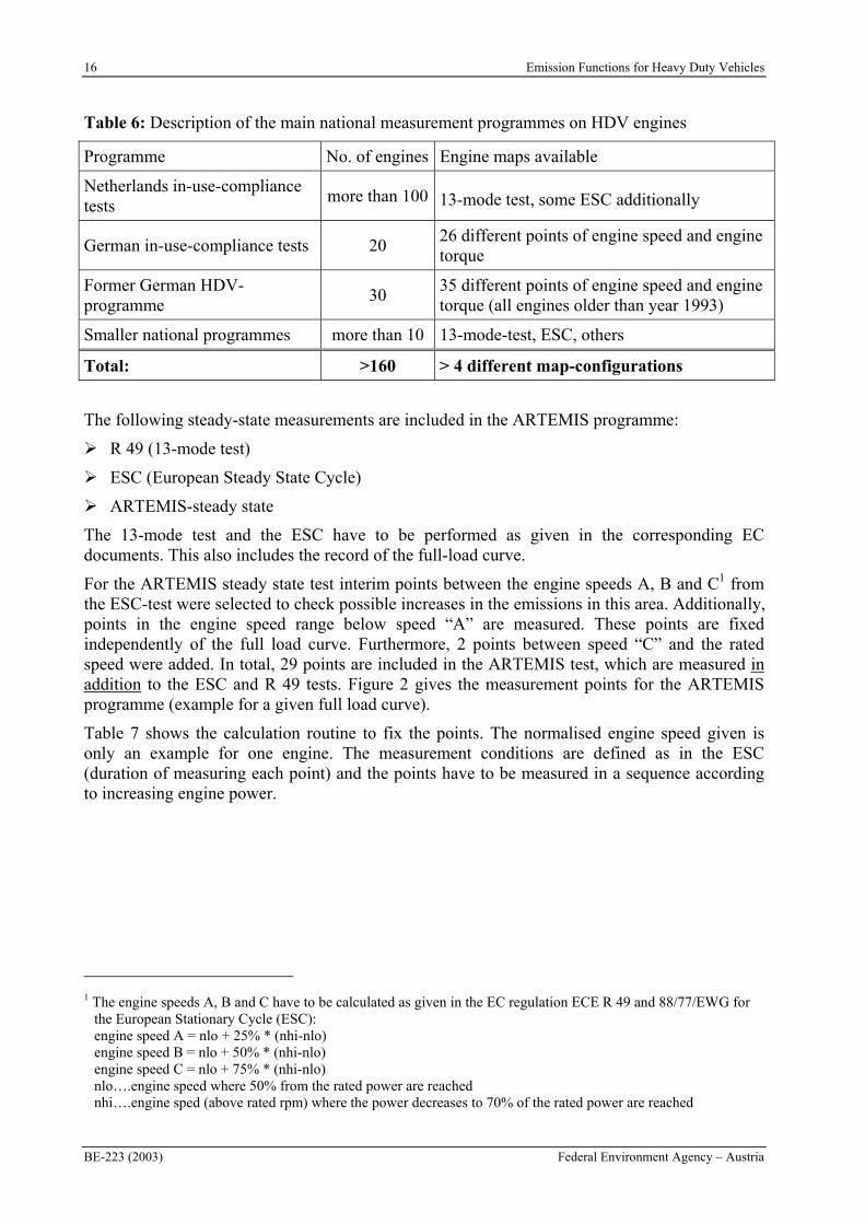
For the ARTEMIS steady state test interim points between the engine speeds A, B and C1 from the ESC-test were selected to check possible increases in the emissions in this area. Additionally, points in the engine speed range below speed “A” are measured. These points are fixed independently of the full load curve. Furthermore, 2 points between speed “C” and the rated speed were added. In total, 29 points are included in the ARTEMIS test, which are measured in addition to the ESC and R 49 tests. Figure 2 gives the measurement points for the ARTEMIS programme (example for a given full load curve).
Table 7 shows the calculation routine to fix the points. The normalised engine speed given is only an example for one engine. The measurement conditions are defined as in the ESC (duration of measuring each point) and the points have to be measured in a sequence according to increasing engine power.
1 The engine speeds A, B and C have to be calculated as given in the EC regulation ECE R 49 and 88/77/EWG for the European Stationary Cycle (ESC): engine speed A = nlo + 25% * (nhi-nlo) engine speed B = nlo + 50% * (nhi-nlo) engine speed C = nlo + 75% * (nhi-nlo) nlo….engine speed where 50% from the rated power are reached nhi….engine sped (above rated rpm) where the power decreases to 70% of the rated power are reached
Emission Functions for Heavy Duty Vehicles 17
Federal Environment Agency – Austria BE-223 (2003)
-75
-50
-25
0
25
50
75
100
125
150
175
200
225
250
275
300
325
0% 10% 20% 30% 40% 50% 60% 70% 80% 90% 100% 110%
engine speed [0%...idle, 100%...rated speed]
po
wer
[kW
]full load curve
ARTEMIS Points
ESC
13 mode
Figure 2: Steady-state points measured in the ARTEMIS programme (example)
Table 7: Test points for the ARTEMIS steady-state test(example)
norm. speed normalised Torquen_idle 0.0%
TUG-Interim 0.35*nA 14.3% 10% 25% 50% 75% 100%
TUG-Interim 0.7*nA 28.7% -100% 10% 25% 50% 75% 100%
ESC-A nlo + 0,25*(nhi - nlo) 41.0% 10% 90%
ESC-B nlo + 0,50*(nhi - nlo) 63.0% 10% 90%
ESC-C nlo + 0,75*(nhi - nlo) 85.1% -100% 10% 90%
TUG-Interim 0.4*nA+0.6*nB 54.2% -100% 10% 30% 60% 100%
TUG-Interim 0.6*nB+0.4*nC 71.9% 10% 30% 60% 100%
TUG-Interim nC+(rated speed-nC)/2 92.5% 25% 75%
Explanations:
- 100% : ...........motoring curve
n_norm = (n - n_idle)/(n_rated - n_idle)
18 Emission Functions for Heavy Duty Vehicles
BE-223 (2003) Federal Environment Agency – Austria
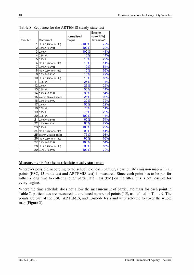
Table 8: Sequence for the ARTEMIS steady-state test
Point Nr. Commentnormalised torque
Engine speed [%] "example"
1 nlo + 0,75*(nhi - nlo) -100% 72%2 0.4*nA+0.6*nB -100% 29%3 0.7*nA -100% 41%4 0.35*nA 10% 14%5 0.7*nA 10% 29%6 nlo + 0,25*(nhi - nlo) 10% 41%7 0.4*nA+0.6*nB 10% 54%8 nlo + 0,50*(nhi - nlo) 10% 63%9 0.6*nB+0.4*nC 10% 72%
10 nlo + 0,75*(nhi - nlo) 10% 85%11 0.35*nA 25% 14%12 0.7*nA 25% 29%13 0.35*nA 50% 14%14 0.4*nA+0.6*nB 30% 54%15 interim C-rated speed 25% 93%16 0.6*nB+0.4*nC 30% 72%17 0.7*nA 50% 29%18 0.35*nA 75% 14%19 0.7*nA 75% 29%20 0.35*nA 100% 14%21 0.4*nA+0.6*nB 60% 54%22 0.6*nB+0.4*nC 60% 72%23 0.7*nA 100% 29%24 nlo + 0,25*(nhi - nlo) 90% 41%25 interim C-rated speed 75% 93%26 nlo + 0,50*(nhi - nlo) 90% 63%27 0.4*nA+0.6*nB 100% 54%28 nlo + 0,75*(nhi - nlo) 90% 85%29 0.6*nB+0.4*nC 100% 72%
Measurements for the particulate steady state map
Wherever possible, according to the schedule of each partner, a particulate emission map with all points (ESC, 13-mode test and ARTEMIS-test) is measured. Since each point has to be run for rather a long time to collect enough particulate mass (PM) on the filter, this is not possible for every engine.
Where the time schedule does not allow the measurement of particulate mass for each point in Table 7, particulates are measured at a reduced number of points (15), as defined in Table 9. The points are part of the ESC, ARTEMIS, and 13-mode tests and were selected to cover the whole map (Figure 3).
Emission Functions for Heavy Duty Vehicles 19
Federal Environment Agency – Austria BE-223 (2003)
-75
-50
-25
0
25
50
75
100
125
150
175
200
225
250
275
300
325
0% 10% 20% 30% 40% 50% 60% 70% 80% 90% 100% 110%
engine speed [0%...idle, 100%...rated speed]
po
wer
[kW
]full load curve
Particle measurements
A CB
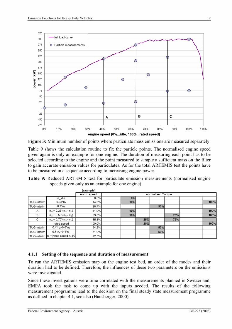
Figure 3: Minimum number of points where particulate mass emissions are measured separately
Table 9 shows the calculation routine to fix the particle points. The normalised engine speed given again is only an example for one engine. The duration of measuring each point has to be selected according to the engine and the point measured to sample a sufficient mass on the filter to gain accurate emission values for particulates. As for the total ARTEMIS test the points have to be measured in a sequence according to increasing engine power.
Table 9: Reduced ARTEMIS test for particulate emission measurements (normalised engine speeds given only as an example for one engine)
(example)norm. speed normalised Torque
n_idle 0.0% 0%TUG-Interim 0.35*nA 14.3% 10% 100%
TUG-Interim 0.7*nA 28.7% 50%
A nlo + 0,25*(nhi - nlo) 41.0% 10% 100%
B nlo + 0,50*(nhi - nlo) 63.0% 10% 75% 100%
C nlo + 0,75*(nhi - nlo) 85.1% 25% 75%
rated speed 100.0% 25% 100%TUG-Interim 0.4*nA+0.6*nB 54.2% 50%
TUG-Interim 0.6*nB+0.4*nC 71.9% 50%
TUG-Interim nC+(rated speed-nC)/2 92.5%
4.1.1 Setting of the sequence and duration of measurement
To run the ARTEMIS emission map on the engine test bed, an order of the modes and their duration had to be defined. Therefore, the influences of these two parameters on the emissions were investigated.
Since these investigations were time correlated with the measurements planned in Switzerland, EMPA took the task to come up with the inputs needed. The results of the following measurement programme lead to the decision on the final steady state measurement programme as defined in chapter 4.1, see also (Hausberger, 2000).
20 Emission Functions for Heavy Duty Vehicles
BE-223 (2003) Federal Environment Agency – Austria
Measurement programme
Three different versions of the ARTEMIS emission maps were performed. In the first one, engine power was increased from mode to mode, in the second one decreased. In both versions, the mode duration was set to 2 minutes like in ESC. In the third version, the mode duration was 5 minutes in order to provide sufficient sampling time for the particulates measurement. Again, engine power was increased from mode to mode.
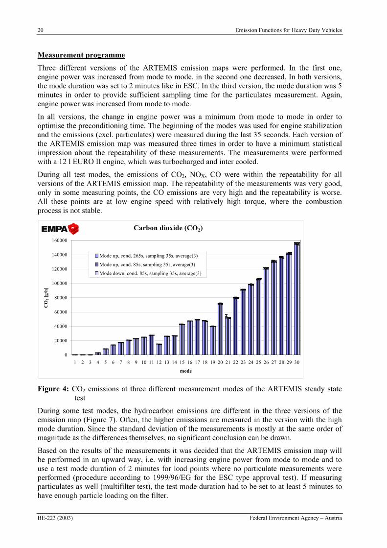
In all versions, the change in engine power was a minimum from mode to mode in order to optimise the preconditioning time. The beginning of the modes was used for engine stabilization and the emissions (excl. particulates) were measured during the last 35 seconds. Each version of the ARTEMIS emission map was measured three times in order to have a minimum statistical impression about the repeatability of these measurements. The measurements were performed with a 12 l EURO II engine, which was turbocharged and inter cooled.
During all test modes, the emissions of CO2, NOX, CO were within the repeatability for all versions of the ARTEMIS emission map. The repeatability of the measurements was very good, only in some measuring points, the CO emissions are very high and the repeatability is worse. All these points are at low engine speed with relatively high torque, where the combustion process is not stable.
Carbon dioxide (CO2)
0
20000
40000
60000
80000
100000
120000
140000
160000
1 2 3 4 5 6 7 8 9 10 11 12 13 14 15 16 17 18 19 20 21 22 23 24 25 26 27 28 29 30
mode
CO
2 [g
/h]
Mode up, cond. 265s, sampling 35s, average(3)
Mode up, cond. 85s, sampling 35s, average(3)
Mode down, cond. 85s, sampling 35s, average(3)
Figure 4: CO2 emissions at three different measurement modes of the ARTEMIS steady state test
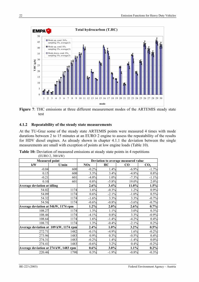
During some test modes, the hydrocarbon emissions are different in the three versions of the emission map (Figure 7). Often, the higher emissions are measured in the version with the high mode duration. Since the standard deviation of the measurements is mostly at the same order of magnitude as the differences themselves, no significant conclusion can be drawn.
Based on the results of the measurements it was decided that the ARTEMIS emission map will be performed in an upward way, i.e. with increasing engine power from mode to mode and to use a test mode duration of 2 minutes for load points where no particulate measurements were performed (procedure according to 1999/96/EG for the ESC type approval test). If measuring particulates as well (multifilter test), the test mode duration had to be set to at least 5 minutes to have enough particle loading on the filter.
Emission Functions for Heavy Duty Vehicles 21
Federal Environment Agency – Austria BE-223 (2003)
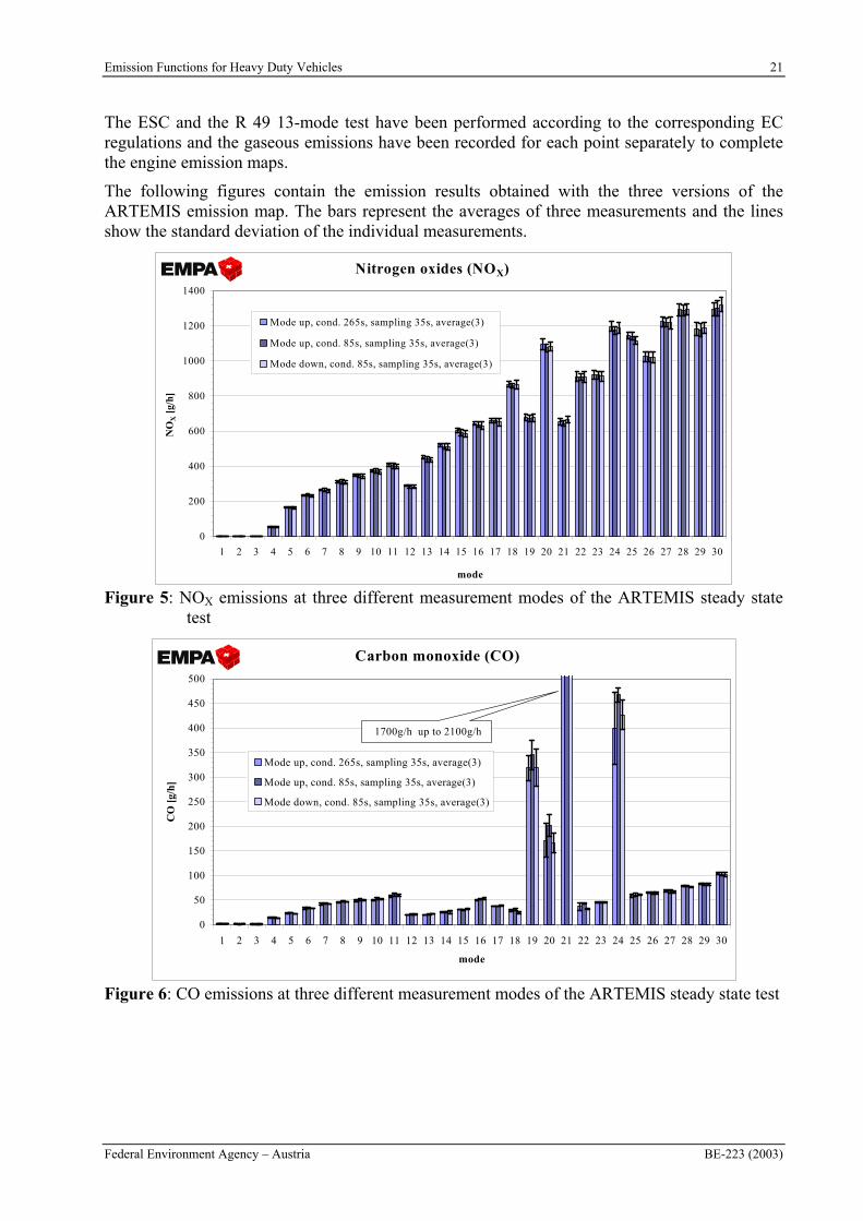
The ESC and the R 49 13-mode test have been performed according to the corresponding EC regulations and the gaseous emissions have been recorded for each point separately to complete the engine emission maps.
The following figures contain the emission results obtained with the three versions of the ARTEMIS emission map. The bars represent the averages of three measurements and the lines show the standard deviation of the individual measurements.
Nitrogen oxides (NOX)
0
200
400
600
800
1000
1200
1400
1 2 3 4 5 6 7 8 9 10 11 12 13 14 15 16 17 18 19 20 21 22 23 24 25 26 27 28 29 30
mode
NO
X [
g/h
]
Mode up, cond. 265s, sampling 35s, average(3)
Mode up, cond. 85s, sampling 35s, average(3)
Mode down, cond. 85s, sampling 35s, average(3)
Figure 5: NOX emissions at three different measurement modes of the ARTEMIS steady state test
Carbon monoxide (CO)
0
50
100
150
200
250
300
350
400
450
500
1 2 3 4 5 6 7 8 9 10 11 12 13 14 15 16 17 18 19 20 21 22 23 24 25 26 27 28 29 30
mode
CO
[g/
h]
Mode up, cond. 265s, sampling 35s, average(3)
Mode up, cond. 85s, sampling 35s, average(3)
Mode down, cond. 85s, sampling 35s, average(3)
1700g/h up to 2100g/h
Figure 6: CO emissions at three different measurement modes of the ARTEMIS steady state test
22 Emission Functions for Heavy Duty Vehicles
BE-223 (2003) Federal Environment Agency – Austria
Total hydrocarbon (T.HC)
0
5
10
15
20
25
30
35
40
45
50
1 2 3 4 5 6 7 8 9 10 11 12 13 14 15 16 17 18 19 20 21 22 23 24 25 26 27 28 29 30
mode
T.H
C [
g/h
]
Mode up, cond. 265s,sampling 35s, average(3)
Mode up, cond. 85s,sampling 35s, average(3)
Mode down, cond. 85s,sampling 35s, average(3)
Figure 7: THC emissions at three different measurement modes of the ARTEMIS steady state test
4.1.2 Repeatability of the steady state measurements
At the TU-Graz some of the steady state ARTEMIS points were measured 4 times with mode durations between 2 to 15 minutes at an EURO 2 engine to assess the repeatability of the results for HDV diesel engines. As already shown in chapter 4.1.1 the deviation between the single measurements are small with exception of points at low engine loads (Table 10).
Table 10: Deviation of measured emissions at steady state points in 4 repetitions(EURO 2, 300 kW)
Measured point Deviation to average measured value kW U/min NOx HC CO CO2
-0.04 600 -0.2% 1.4% -6.9% -1.7%0.15 600 3.3% 3.4% -4.8% 0.8%
-0.21 601 -4.0% 1.0% -7.3% -1.1%0.10 601 0.8% -5.8% 19.0% 2.0%
Average deviation at idling 2.6% 3.4% 11.0% 1.5%54.02 1174 1.6% -0.3% 1.2% 0.9%54.09 1174 0.6% -2.1% -1.0% 0.5%54.32 1174 -1.6% 3.3% 3.3% -0.7%54.56 1174 -0.6% -0.8% -3.6% -0.7%
Average deviation at 54kW, 1174 rpm 1.2% 2.0% 2.6% 0.7%108.27 1174 1.3% 1.1% 3.0% 0.3%108.46 1174 -4.1% 0.8% 3.3% -0.9%108.64 1174 1.6% -1.4% -4.2% 0.4%108.73 1174 1.3% -0.4% -2.1% 0.2%
Average deviation at 109 kW, 1174 rpm 2.4% 1.0% 3.2% 0.5%272.71 1482 -0.1% -4.9% 1.6% -0.2%273.96 1483 0.9% 0.3% -0.5% 0.4%274.31 1483 -0.2% 1.4% -1.4% 0.0%274.41 1483 -0.6% 3.2% 0.4% -0.2%
Average deviation at 274 kW, 1483 rpm 0.6% 3.0% 1.1% 0.2%220.46 1790 0.3% -1.9% -0.8% -0.3%
Emission Functions for Heavy Duty Vehicles 23
Federal Environment Agency – Austria BE-223 (2003)
222.34 1791 -0.7% 2.3% 1.3% -0.6%220.86 1791 -0.3% -1.2% 0.4% 0.5%221.29 1791 0.7% 0.8% -1.0% 0.4%
Average deviation at 221 kW, 1791 rpm 0.5% 1.6% 1.0% 0.5%
4.1.3 Assessment of the steady state measurements
The assessment of the measured steady state engine maps shows that it is essential for the elaboration of real world emission factors for modern engines to use off-cycle measurements as well. Since electronic engine control systems – used from EURO 2 levels on - allow different injection timings over the engine map, optimisations in the specific fuel consumption can result in increased NOx emissions outside of the homologation test points. Actual common rail injection systems in EURO 3 engines give additional degrees of freedom e.g. from the rail-pressure and the possibility for pre-injection and post-injection what offers also possibilities for influencing the particle emissions differently within the engine map.
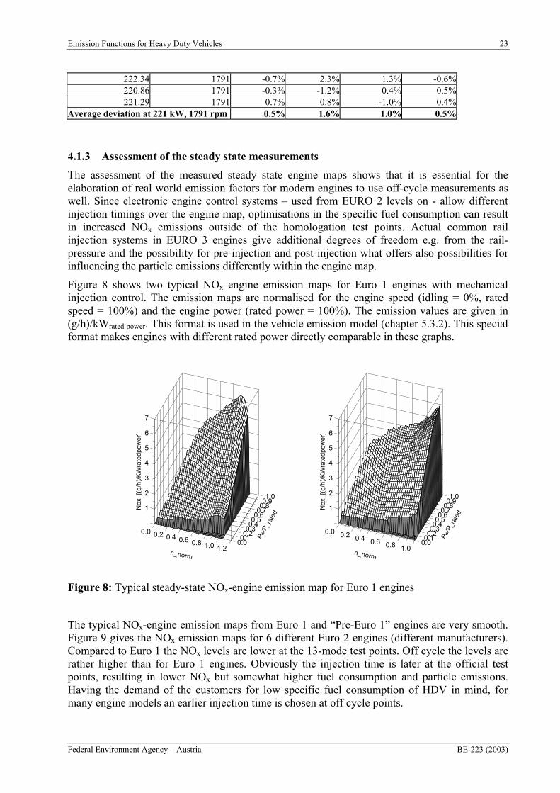
Figure 8 shows two typical NOx engine emission maps for Euro 1 engines with mechanical injection control. The emission maps are normalised for the engine speed (idling = 0%, rated speed = 100%) and the engine power (rated power = 100%). The emission values are given in (g/h)/kWrated power. This format is used in the vehicle emission model (chapter 5.3.2). This special format makes engines with different rated power directly comparable in these graphs.
0.0 0.2 0.4 0.6 0.8 1.0 1.2n_norm
0.00.10.20.30.40.50.60.70.80.91.0
Pe/
P_r
ated
1
2
3
4
5
6
7
No
x_[(
g/h
)/K
Wra
tedp
ow
er]
0.0 0.2 0.4 0.6 0.8 1.0n_norm
0.00.10.20.30.40.50.60.70.80.91.0
Pe/
P_r
ated
1
2
3
4
5
6
7
No
x_[(
g/h
)/K
Wra
tedp
ow
er]
Figure 8: Typical steady-state NOx-engine emission map for Euro 1 engines
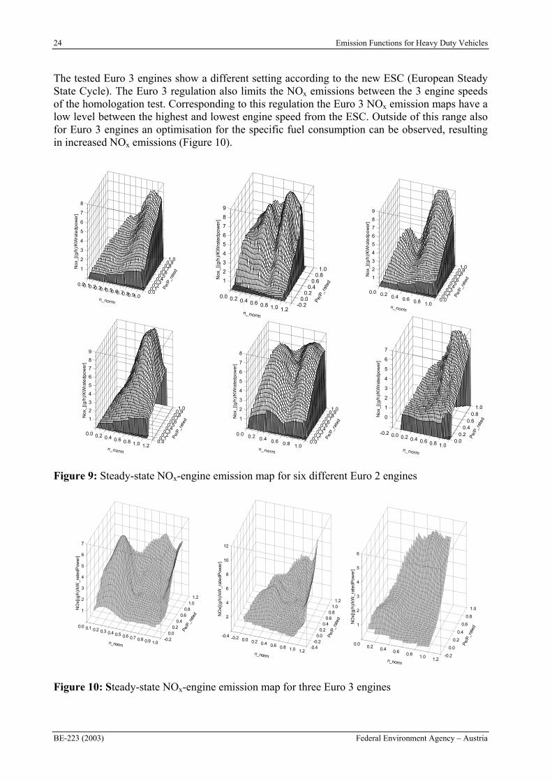
The typical NOx-engine emission maps from Euro 1 and “Pre-Euro 1” engines are very smooth. Figure 9 gives the NOx emission maps for 6 different Euro 2 engines (different manufacturers). Compared to Euro 1 the NOx levels are lower at the 13-mode test points. Off cycle the levels are rather higher than for Euro 1 engines. Obviously the injection time is later at the official test points, resulting in lower NOx but somewhat higher fuel consumption and particle emissions. Having the demand of the customers for low specific fuel consumption of HDV in mind, for many engine models an earlier injection time is chosen at off cycle points.
24 Emission Functions for Heavy Duty Vehicles
BE-223 (2003) Federal Environment Agency – Austria
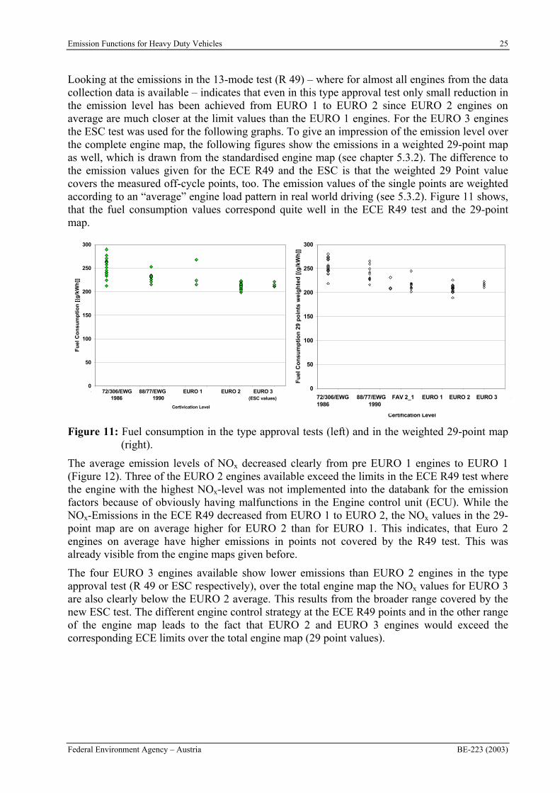
The tested Euro 3 engines show a different setting according to the new ESC (European Steady State Cycle). The Euro 3 regulation also limits the NOx emissions between the 3 engine speeds of the homologation test. Corresponding to this regulation the Euro 3 NOx emission maps have a low level between the highest and lowest engine speed from the ESC. Outside of this range also for Euro 3 engines an optimisation for the specific fuel consumption can be observed, resulting in increased NOx emissions (Figure 10).
0.00.10.20.30.40.50.60.70.80.91.0n_norm
0.00.10.20.30.40.50.60.70.80.91.0
Pe/
P_r
ated
1
2
3
4
5
6
7
8
No
x_[(
g/h
)/K
Wra
ted
po
we
r]
0.0 0.2 0.4 0.6 0.8 1.0n_norm
0.00.10.20.30.40.50.60.70.80.91.0
Pe/
P_r
ated
1
2
3
4
5
6
7
8
9
No
x_[(
g/h
)/K
Wra
ted
po
we
r]
0.0 0.2 0.4 0.6 0.8 1.0 1.2n_norm
0.00.10.20.30.40.50.60.70.80.91.0
Pe/
P_r
ated
1
2
3
4
5
6
7
8
9
No
x_[(
g/h
)/K
Wra
ted
pow
er]
0.0 0.2 0.4 0.6 0.8 1.0n_norm
0.00.10.20.30.40.50.60.70.80.91.0
Pe/
P_r
ated
1
2
3
4
5
6
7
8
No
x_[(
g/h
)/K
Wra
ted
po
we
r]
0.0 0.2 0.4 0.6 0.8 1.0 1.2n_norm
-0.20.0
0.20.4
0.60.8
1.0
Pe/
P_r
ated
1
2
3
4
5
6
7
8
9
Nox
_[(
g/h)
/KW
rate
dpo
we
r]
-0.2 0.0 0.2 0.4 0.6 0.8 1.0n_norm
0.00.2
0.40.6
0.81.0
Pe/
P_ra
ted0
1
2
3
4
5
6
7
No
x_[(
g/h
)/K
Wra
ted
pow
er]
Figure 9: Steady-state NOx-engine emission map for six different Euro 2 engines
-0.20.0
0.20.4
0.60.8
1.01.2
Pe/P
_rat
ed
0.0 0.1 0.2 0.3 0.4 0.5 0.6 0.7 0.8 0.9 1.0n_norm
1
2
3
4
5
6
7
NO
x[(g
/h)/
kW_r
ated
Pow
er]
-0.4-0.2
0.00.2
0.40.6
0.81.0
1.2
Pe/
P_r
ated
-0.4 -0.2 0.0 0.2 0.4 0.6 0.8 1.0 1.2n_norm
2
4
6
8
10
12
NO
x[(g
/h)/
kW_r
ated
Pow
er]
-0.2
0.0
0.2
0.4
0.6
0.8
1.0
Pe/
P_r
ated
0.00.2 0.4 0.6 0.8
1.0 1.2n_norm
1
2
3
4
5
6
NO
x[(g
/h)/
kW_r
ated
Pow
er]
Figure 10: Steady-state NOx-engine emission map for three Euro 3 engines
Emission Functions for Heavy Duty Vehicles 25
Federal Environment Agency – Austria BE-223 (2003)
Looking at the emissions in the 13-mode test (R 49) – where for almost all engines from the data collection data is available – indicates that even in this type approval test only small reduction in the emission level has been achieved from EURO 1 to EURO 2 since EURO 2 engines on average are much closer at the limit values than the EURO 1 engines. For the EURO 3 engines the ESC test was used for the following graphs. To give an impression of the emission level over the complete engine map, the following figures show the emissions in a weighted 29-point map as well, which is drawn from the standardised engine map (see chapter 5.3.2). The difference to the emission values given for the ECE R49 and the ESC is that the weighted 29 Point value covers the measured off-cycle points, too. The emission values of the single points are weighted according to an “average” engine load pattern in real world driving (see 5.3.2). Figure 11 shows, that the fuel consumption values correspond quite well in the ECE R49 test and the 29-point map.
0
50
100
150
200
250
300
1985 1987 1989 1991 1993 1995 1997 1999 2001
Certivication Level
Fu
el C
on
sum
pti
on
[(g
/kW
h]]
72/306/EWG 88/77/EWG EURO 1 EURO 2 EURO 3 1986 1990 (ESC values)
0
50
100
150
200
250
300
1985 1987 1989 1991 1993 1995 1997 1999 2001 2003
Certification Level
Fu
el C
on
sum
pti
on
29
po
ints
wei
gh
ted
[(g
/kW
h]]
72/306/EWG 88/77/EWG FAV 2_1 EURO 1 EURO 2 EURO 3 1986 1990
Figure 11: Fuel consumption in the type approval tests (left) and in the weighted 29-point map (right).
The average emission levels of NOx decreased clearly from pre EURO 1 engines to EURO 1 (Figure 12). Three of the EURO 2 engines available exceed the limits in the ECE R49 test where the engine with the highest NOx-level was not implemented into the databank for the emission factors because of obviously having malfunctions in the Engine control unit (ECU). While the NOx-Emissions in the ECE R49 decreased from EURO 1 to EURO 2, the NOx values in the 29-point map are on average higher for EURO 2 than for EURO 1. This indicates, that Euro 2 engines on average have higher emissions in points not covered by the R49 test. This was already visible from the engine maps given before.
The four EURO 3 engines available show lower emissions than EURO 2 engines in the type approval test (R 49 or ESC respectively), over the total engine map the NOx values for EURO 3 are also clearly below the EURO 2 average. This results from the broader range covered by the new ESC test. The different engine control strategy at the ECE R49 points and in the other range of the engine map leads to the fact that EURO 2 and EURO 3 engines would exceed the corresponding ECE limits over the total engine map (29 point values).
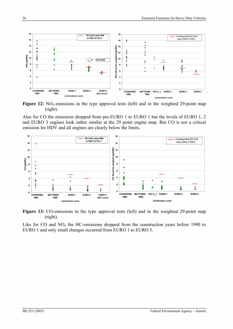
26 Emission Functions for Heavy Duty Vehicles
BE-223 (2003) Federal Environment Agency – Austria
0
2
4
6
8
10
12
14
16
18
1985 1987 1989 1991 1993 1995 1997 1999 2001 2003
Certification Level
NO
x 2
9 p
oin
ts w
eig
hte
d [
g/k
Wh
]
72/306/EWG 88/77/EWG FAV 2_1 EURO 1 EURO 2 EURO 3 1986 1990
corresponding EC limit value (R49 or ESC)
0
2
4
6
8
10
12
14
16
18
1985 1987 1989 1991 1993 1995 1997 1999 2001 2003
Certivication Level
NO
x [g
/kW
h]
72/306/EWG 88/77/EWG EURO 1 EURO 2 EURO 3 1986 1990 (ESC-values)
EC limit value R49 or ESC for EU 3
excluded
Figure 12: NOx-emissions in the type approval tests (left) and in the weighted 29-point map (right).
Also for CO the emissions dropped from pre-EURO 1 to EURO 1 but the levels of EURO 1, 2 and EURO 3 engines look rather similar at the 29 point engine map. But CO is not a critical emission for HDV and all engines are clearly below the limits.
0
2
4
6
8
10
12
14
16
1985 1987 1989 1991 1993 1995 1997 1999 2001 2003
Certification Level
CO
29
po
ints
wei
gh
ted
[g
/kW
h]
72/306/EWG 88/77/EWG FAV 2_1 EURO 1 EURO 2 EURO 3 1986 1990
corresponding EC limit value (R49 or ESC)
0
2
4
6
8
10
12
14
16
1985 1987 1989 1991 1993 1995 1997 1999 2001 2003
Certivication Level
CO
[g
/kW
h]
72/306/EWG 88/77/EWG EURO 1 EURO 2 EURO 3 1986 1990 (ESC-values)
EC limit value R49 or ESC for EU 3
Figure 13: CO-emissions in the type approval tests (left) and in the weighted 29-point map (right).
Like for CO and NOx the HC-emissions dropped from the construction years before 1990 to EURO 1 and only small changes occurred from EURO 1 to EURO 3.
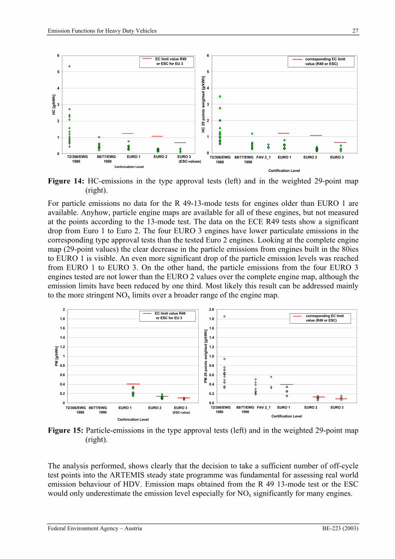
Emission Functions for Heavy Duty Vehicles 27
Federal Environment Agency – Austria BE-223 (2003)
0
1
2
3
4
5
6
1985 1987 1989 1991 1993 1995 1997 1999 2001 2003
Certivication Level
HC
[g
/kW
h]
72/306/EWG 88/77/EWG EURO 1 EURO 2 EURO 3 1986 1990 (ESC-values)
EC limit value R49 or ESC for EU 3
0
1
2
3
4
5
6
1985 1987 1989 1991 1993 1995 1997 1999 2001 2003
Certification Level
HC
29
po
ints
wei
gh
ted
[g
/kW
h]
72/306/EWG 88/77/EWG FAV 2_1 EURO 1 EURO 2 EURO 3 1986 1990
corresponding EC limit value (R49 or ESC)
Figure 14: HC-emissions in the type approval tests (left) and in the weighted 29-point map (right).
For particle emissions no data for the R 49-13-mode tests for engines older than EURO 1 are available. Anyhow, particle engine maps are available for all of these engines, but not measured at the points according to the 13-mode test. The data on the ECE R49 tests show a significant drop from Euro 1 to Euro 2. The four EURO 3 engines have lower particulate emissions in the corresponding type approval tests than the tested Euro 2 engines. Looking at the complete engine map (29-point values) the clear decrease in the particle emissions from engines built in the 80ies to EURO 1 is visible. An even more significant drop of the particle emission levels was reached from EURO 1 to EURO 3. On the other hand, the particle emissions from the four EURO 3 engines tested are not lower than the EURO 2 values over the complete engine map, although the emission limits have been reduced by one third. Most likely this result can be addressed mainly to the more stringent NOx limits over a broader range of the engine map.
0
0.2
0.4
0.6
0.8
1
1.2
1.4
1.6
1.8
2
1985 1987 1989 1991 1993 1995 1997 1999 2001 2003
Certivication Level
PM
[g
/kW
h]
72/306/EWG 88/77/EWG EURO 1 EURO 2 EURO 3 1986 1990 (ESC-value)
EC limit value R49 or ESC for EU 3
0.0
0.2
0.4
0.6
0.8
1.0
1.2
1.4
1.6
1.8
2.0
1985 1987 1989 1991 1993 1995 1997 1999 2001 2003
Certification Level
PM
29
po
ints
we
igh
ted
[g
/kW
h]
72/306/EWG 88/77/EWG FAV 2_1 EURO 1 EURO 2 EURO 3 1986 1990
corresponding EC limit value (R49 or ESC)
Figure 15: Particle-emissions in the type approval tests (left) and in the weighted 29-point map (right).
The analysis performed, shows clearly that the decision to take a sufficient number of off-cycle test points into the ARTEMIS steady state programme was fundamental for assessing real world emission behaviour of HDV. Emission maps obtained from the R 49 13-mode test or the ESC would only underestimate the emission level especially for NOx significantly for many engines.
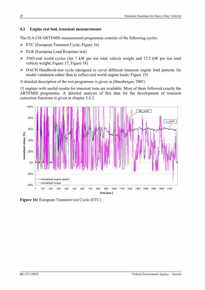
28 Emission Functions for Heavy Duty Vehicles
BE-223 (2003) Federal Environment Agency – Austria
4.2 Engine test bed, transient measurements
The D.A.CH/ARTEMIS measurement programme consists of the following cycles:
ETC (European Transient Cycle, Figure 16)
ELR (European Load Response test)
TNO-real world cycles (for 7 kW per ton total vehicle weight and 12.5 kW per ton total vehicle weight; Figure 17, Figure 18)
DACH-Handbook-test cycle (designed to cover different transient engine load patterns for model validation rather than to reflect real world engine loads; Figure 19)
A detailed description of the test programme is given in (Hausberger, 2001)
13 engines with useful results for transient tests are available. Most of them followed exactly the ARTEMIS programme. A detailed analysis of this data for the development of transient correction functions is given in chapter 5.4.2.
-40%
-20%
0%
20%
40%
60%
80%
100%
1 101 201 301 401 501 601 701 801 901 1001 1101 1201 1301 1401 1501 1601 1701
Time [sec.]
no
rmal
ised
val
ues
[%
]
normalised engine speed
normalised torque
n_norm
Md_norm
Figure 16: European Transient test Cycle (ETC)

Emission Functions for Heavy Duty Vehicles 29
Federal Environment Agency – Austria BE-223 (2003)
-40
-20
0
20
40
60
80
100
120
1 201 401 601 801 1001 1201 1401 1601 1801 2001 2201 2401 2601 2801 3001 3201 3401 3601 3801
Time [sec.]
no
rmal
ised
val
ues
[%
]
Normalised speed [%]
Normalised Torque [%]
n_norm
Figure 17: TNO real world test Cycle (12.5 kW/ton)
-40
-20
0
20
40
60
80
100
1 201 401 601 801 1001 1201 1401 1601 1801 2001 2201 2401 2601 2801 3001 3201 3401 3601 3801
Time [sec.]
no
rmal
ised
val
ues
[%
]
Normalised speed [%]
Normalised Torque [%]
n_norm
Figure 18: TNO real world test Cycle (7 kW/ton)
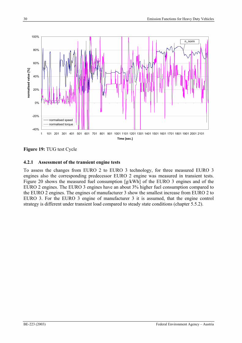
30 Emission Functions for Heavy Duty Vehicles
BE-223 (2003) Federal Environment Agency – Austria
-40%
-20%
0%
20%
40%
60%
80%
100%
1 101 201 301 401 501 601 701 801 901 1001 1101 1201 1301 1401 1501 1601 1701 1801 1901 2001 2101
Time [sec.]
no
rmal
ised
val
ue
[%]
normalised speed
normalised torque
n_norm
Figure 19: TUG test Cycle
4.2.1 Assessment of the transient engine tests
To assess the changes from EURO 2 to EURO 3 technology, for three measured EURO 3 engines also the corresponding predecessor EURO 2 engine was measured in transient tests. Figure 20 shows the measured fuel consumption [g/kWh] of the EURO 3 engines and of the EURO 2 engines. The EURO 3 engines have an about 3% higher fuel consumption compared to the EURO 2 engines. The engines of manufacturer 3 show the smallest increase from EURO 2 to EURO 3. For the EURO 3 engine of manufacturer 3 it is assumed, that the engine control strategy is different under transient load compared to steady state conditions (chapter 5.5.2).
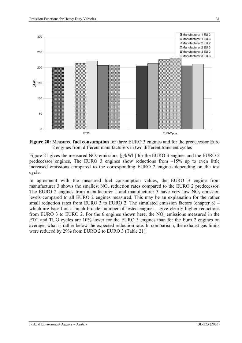
Emission Functions for Heavy Duty Vehicles 31
Federal Environment Agency – Austria BE-223 (2003)
0
50
100
150
200
250
300
ETC TUG-Cycle
g/k
Wh
Manufacturer 1 EU 2
Manufacturer 1 EU 3
Manufacturer 2 EU 2
Manufacturer 2 EU 3
Manufacturer 3 EU 2
Manufacturer 3 EU 3
Figure 20: Measured fuel consumption for three EURO 3 engines and for the predecessor Euro 2 engines from different manufacturers in two different transient cycles
Figure 21 gives the measured NOx-emissions [g/kWh] for the EURO 3 engines and the EURO 2 predecessor engines. The EURO 3 engines show reductions from –15% up to even little increased emissions compared to the corresponding EURO 2 engines depending on the test cycle.
In agreement with the measured fuel consumption values, the EURO 3 engine from manufacturer 3 shows the smallest NOx reduction rates compared to the EURO 2 predecessor. The EURO 2 engines from manufacturer 1 and manufacturer 3 have very low NOx emission levels compared to all EURO 2 engines measured. This may be an explanation for the rather small reduction rates from EURO 3 to EURO 2. The simulated emission factors (chapter 8) – which are based on a much broader number of tested engines - give clearly higher reductions from EURO 3 to EURO 2. For the 6 engines shown here, the NOx emissions measured in the ETC and TUG cycles are 10% lower for the EURO 3 engines than for the Euro 2 engines on average, what is rather below the expected reduction rate. In comparison, the exhaust gas limits were reduced by 29% from EURO 2 to EURO 3 (Table 21).
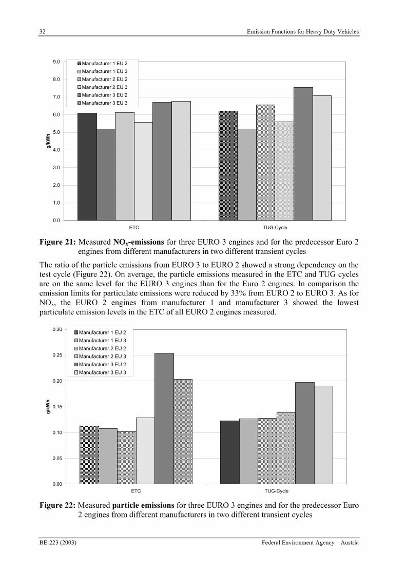
32 Emission Functions for Heavy Duty Vehicles
BE-223 (2003) Federal Environment Agency – Austria
0.0
1.0
2.0
3.0
4.0
5.0
6.0
7.0
8.0
9.0
ETC TUG-Cycle
g/k
Wh
Manufacturer 1 EU 2
Manufacturer 1 EU 3
Manufacturer 2 EU 2
Manufacturer 2 EU 3
Manufacturer 3 EU 2
Manufacturer 3 EU 3
Figure 21: Measured NOx-emissions for three EURO 3 engines and for the predecessor Euro 2 engines from different manufacturers in two different transient cycles
The ratio of the particle emissions from EURO 3 to EURO 2 showed a strong dependency on the test cycle (Figure 22). On average, the particle emissions measured in the ETC and TUG cycles are on the same level for the EURO 3 engines than for the Euro 2 engines. In comparison the emission limits for particulate emissions were reduced by 33% from EURO 2 to EURO 3. As for NOx, the EURO 2 engines from manufacturer 1 and manufacturer 3 showed the lowest particulate emission levels in the ETC of all EURO 2 engines measured.
0.00
0.05
0.10
0.15
0.20
0.25
0.30
ETC TUG-Cycle
g/k
Wh
Manufacturer 1 EU 2
Manufacturer 1 EU 3
Manufacturer 2 EU 2
Manufacturer 2 EU 3
Manufacturer 3 EU 2
Manufacturer 3 EU 3
Figure 22: Measured particle emissions for three EURO 3 engines and for the predecessor Euro 2 engines from different manufacturers in two different transient cycles
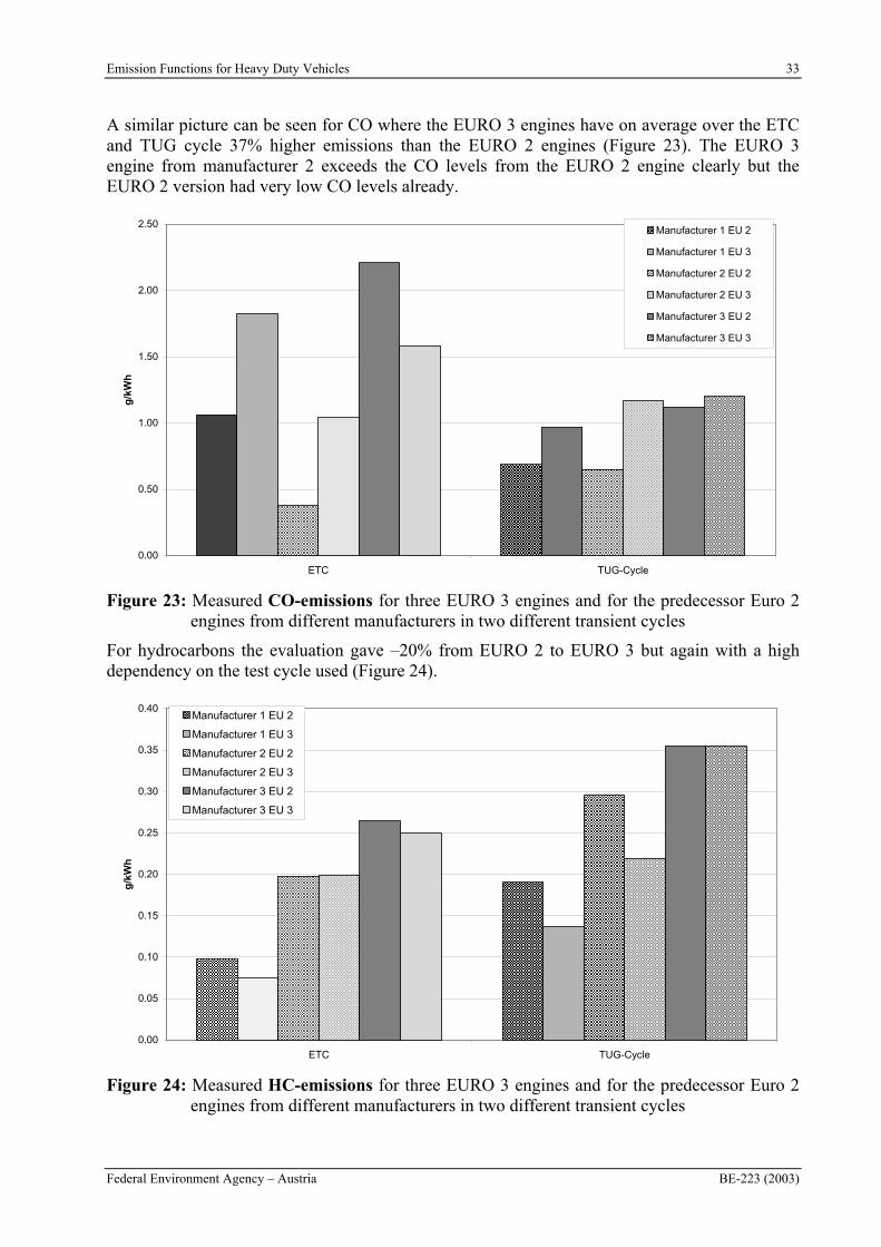
Emission Functions for Heavy Duty Vehicles 33
Federal Environment Agency – Austria BE-223 (2003)
A similar picture can be seen for CO where the EURO 3 engines have on average over the ETC and TUG cycle 37% higher emissions than the EURO 2 engines (Figure 23). The EURO 3 engine from manufacturer 2 exceeds the CO levels from the EURO 2 engine clearly but the EURO 2 version had very low CO levels already.
0.00
0.50
1.00
1.50
2.00
2.50
ETC TUG-Cycle
g/k
Wh
Manufacturer 1 EU 2
Manufacturer 1 EU 3
Manufacturer 2 EU 2
Manufacturer 2 EU 3
Manufacturer 3 EU 2
Manufacturer 3 EU 3
Figure 23: Measured CO-emissions for three EURO 3 engines and for the predecessor Euro 2 engines from different manufacturers in two different transient cycles
For hydrocarbons the evaluation gave –20% from EURO 2 to EURO 3 but again with a high dependency on the test cycle used (Figure 24).
0.00
0.05
0.10
0.15
0.20
0.25
0.30
0.35
0.40
ETC TUG-Cycle
g/k
Wh
Manufacturer 1 EU 2
Manufacturer 1 EU 3
Manufacturer 2 EU 2
Manufacturer 2 EU 3
Manufacturer 3 EU 2
Manufacturer 3 EU 3
Figure 24: Measured HC-emissions for three EURO 3 engines and for the predecessor Euro 2 engines from different manufacturers in two different transient cycles
34 Emission Functions for Heavy Duty Vehicles
BE-223 (2003) Federal Environment Agency – Austria
The transient tests showed approximately the results already expected from the assessment of the steady state engine tests. Later on in the report a detailed comparison of steady state measurements and the transient tests is given (chapter 5.4).
4.3 Chassis dynamometer measurements
The tests on the HDV-chassis dynamometer were mainly performed for model development and model evaluation (chapter 5.5). The engines are tested on the engine test bed according to the D.A.CH./ARTEMIS programme, then the engine is fitted into the HDV again and the tests on the chassis dynamometer are performed. This gives the whole chain for model development from steady state emission maps and transient engine tests to the simulation of HDV driving cycles.
To cover a broad range of relevant driving situations for the model validation, the following driving cycles have been measured:
2 urban cycles: medium dynamic high dynamic
3 rural cycles: low dynamic medium dynamic high dynamic
3 highway cycles: low dynamic medium dynamic high dynamic
The cycles are taken from the Handbook on Emission Factors (Steven, 1995) and were selected after model runs with PHEM (chapter 5), according to the calculated engine load, changes of the engine load (dynamics) and the vehicle speed respectively to cover low-speed to high-speed cycles and low-dynamic to high-dynamic cycles. Figure 25 shows the speed curve of these cycles which are measured with 0% road gradient simulation.
Additionally, constant speeds are measured, whereby the vehicle speed and the driving resistances are adapted to measured points on the engine test bed. This allowed an assessment of the potential inaccuracy related to different measurement systems and different boundary conditions compared to the tests on the engine test bed (chapter 5.5.3).
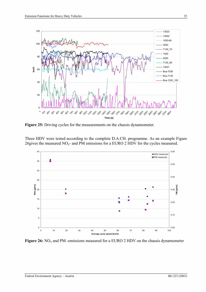
Emission Functions for Heavy Duty Vehicles 35
Federal Environment Agency – Austria BE-223 (2003)
0
20
40
60
80
100
120
110
120
130
140
150
160
170
180
190
110
0111
0112
0113
0114
0115
0116
0117
0118
0119
0120
0121
0122
0123
0124
0125
0126
0127
0128
01
Time [s]
km/h
13023
14022
1020-60
3020
7130_70
1020
2020
7130_85
14021
Bus-7030
Bus-7130
Bus-1020_100
Figure 25: Driving cycles for the measurements on the chassis dynamometer.
Three HDV were tested according to the complete D.A.CH. programme. As an example Figure 26gives the measured NOx- and PM emissions for a EURO 2 HDV for the cycles measured.
0
5
10
15
20
25
30
35
40
0 10 20 30 40 50 60 70 80 90 100
Average cycle speed [km/h]
NO
x [
g/k
m]
0.00
0.10
0.20
0.30
0.40
0.50
0.60
PM
[g
/km
]
NOx measured
PM measured
Figure 26: NOx and PM -emissions measured for a EURO 2 HDV on the chassis dynamometer
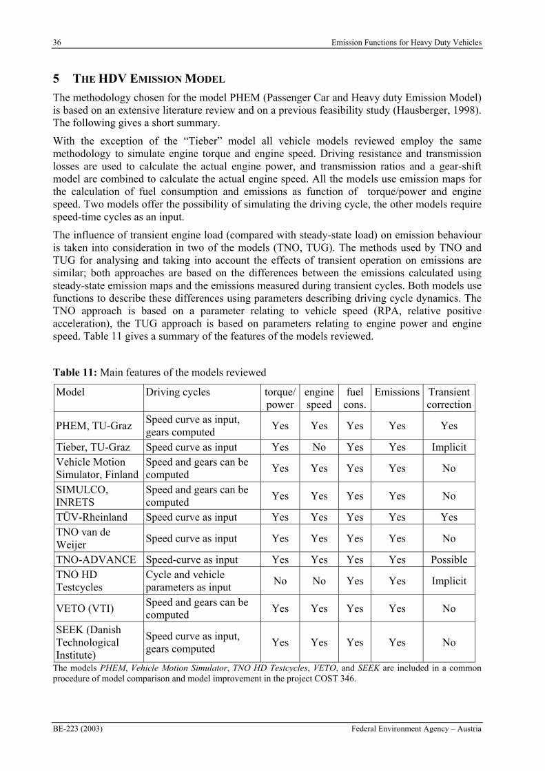
36 Emission Functions for Heavy Duty Vehicles
BE-223 (2003) Federal Environment Agency – Austria
5 THE HDV EMISSION MODEL
The methodology chosen for the model PHEM (Passenger Car and Heavy duty Emission Model) is based on an extensive literature review and on a previous feasibility study (Hausberger, 1998). The following gives a short summary.
With the exception of the “Tieber” model all vehicle models reviewed employ the same methodology to simulate engine torque and engine speed. Driving resistance and transmission losses are used to calculate the actual engine power, and transmission ratios and a gear-shift model are combined to calculate the actual engine speed. All the models use emission maps for the calculation of fuel consumption and emissions as function of torque/power and engine speed. Two models offer the possibility of simulating the driving cycle, the other models require speed-time cycles as an input.
The influence of transient engine load (compared with steady-state load) on emission behaviour is taken into consideration in two of the models (TNO, TUG). The methods used by TNO and TUG for analysing and taking into account the effects of transient operation on emissions are similar; both approaches are based on the differences between the emissions calculated using steady-state emission maps and the emissions measured during transient cycles. Both models use functions to describe these differences using parameters describing driving cycle dynamics. The TNO approach is based on a parameter relating to vehicle speed (RPA, relative positive acceleration), the TUG approach is based on parameters relating to engine power and engine speed. Table 11 gives a summary of the features of the models reviewed.
Table 11: Main features of the models reviewed
Model Driving cycles torque/ power
enginespeed
fuelcons.
Emissions Transient correction
PHEM, TU-Graz Speed curve as input, gears computed
Yes Yes Yes Yes Yes
Tieber, TU-Graz Speed curve as input Yes No Yes Yes Implicit Vehicle Motion Simulator, Finland
Speed and gears can be computed
Yes Yes Yes Yes No
SIMULCO,INRETS
Speed and gears can be computed
Yes Yes Yes Yes No
TÜV-Rheinland Speed curve as input Yes Yes Yes Yes Yes TNO van de Weijer
Speed curve as input Yes Yes Yes Yes No
TNO-ADVANCE Speed-curve as input Yes Yes Yes Yes Possible TNO HD Testcycles
Cycle and vehicle parameters as input
No No Yes Yes Implicit
VETO (VTI) Speed and gears can be computed
Yes Yes Yes Yes No
SEEK (Danish TechnologicalInstitute)
Speed curve as input, gears computed
Yes Yes Yes Yes No
The models PHEM, Vehicle Motion Simulator, TNO HD Testcycles, VETO, and SEEK are included in a common procedure of model comparison and model improvement in the project COST 346.
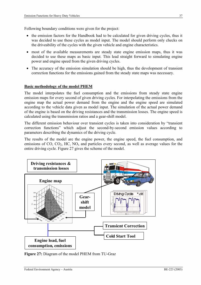
Emission Functions for Heavy Duty Vehicles 37
Federal Environment Agency – Austria BE-223 (2003)
Following boundary conditions were given for the project:
the emission factors for the Handbook had to be calculated for given driving cycles, thus it was decided to use these cycles as model input. The model should perform only checks on the driveability of the cycles with the given vehicle and engine characteristics.
most of the available measurements are steady state engine emission maps, thus it was decided to use these maps as basic input. This lead straight forward to simulating engine power and engine speed from the given driving cycles.
The accuracy of the emission simulation should be high, thus the development of transient correction functions for the emissions gained from the steady state maps was necessary.
Basic methodology of the model PHEM
The model interpolates the fuel consumption and the emissions from steady state engine emission maps for every second of given driving cycles. For interpolating the emissions from the engine map the actual power demand from the engine and the engine speed are simulated according to the vehicle data given as model input. The simulation of the actual power demand of the engine is based on the driving resistances and the transmission losses. The engine speed is calculated using the transmission ratios and a gear-shift model.
The different emission behaviour over transient cycles is taken into consideration by “transient correction functions” which adjust the second-by-second emission values according to parameters describing the dynamics of the driving cycle.
The results of the model are the engine power, the engine speed, the fuel consumption, and emissions of CO, CO2, HC, NOx and particles every second, as well as average values for the entire driving cycle. Figure 27 gives the scheme of the model.
Engine load, fuel consumption, emissions
Engine map
Driving resistances &transmission losses
Gear-shift
model
Transient Correction
Cold Start ToolCold Start Tool
0.00.2
0.40.6
0.81.0
n_norm
-0.20.0
0.20.4
0.60.8
1.0
Pe/P_rated
50
100
150
200
250
FC
Figure 27: Diagram of the model PHEM from TU-Graz
38 Emission Functions for Heavy Duty Vehicles
BE-223 (2003) Federal Environment Agency – Austria
While this method is common for most models compared (with exception of the transient correction function), the model PHEM has some special features developed straight forward to enable easy simulations of average HDV classes.
The input data is modular, i.e. different files for
The vehicle characterisation
The driving cycle
The engine emission map
The full load curve
This enables a quick simulation of manifold vehicle / driving cycle combinations.
A main problem in the elaboration of emission factors for average HDV is to have a sufficient number of engines measured for each HDV fleet segment because overall more than 60 segments of the fleet have to be covered. A “fleet segment” is defined here as the combination of a vehicle type (e.g. single truck or truck trailer) with a EURO category (e.g. EURO 3) and a size class (e.g. 34-40 tons maximum allowed payload). Since each size class has its typical values for the rated engine power, each measured engine basically can be applied to one fleet segment only.
To avoid a separation of the measured engines according to the rated engine power, the engine maps are normalized and brought into a standard format (see chapter 5.3.2). This enables the development of average engine maps independent of the engine size. Without this method of averaging emission maps, even the high number of measured engine maps available for the project would leave some “HDV-layers” covered by one engine only (or even without an appropriate engine at all). The method of size independent averaging guarantees that the single HDV classes are covered by a proper number of measurements of different engines.
In the input file for the driving cycle the measured engine speed or the gear position can be given as optional model input. If neither the engine speed nor the gear position is given in the input file, PHEM uses the gear-shift model to simulate the engine speed. When recalculating driving cycles measured at the chassis dynamometer differences between simulated and measured emissions related to differences in the gear-shift strategy can be addressed exactly. This is a helpful tool in model development and model validation.
For the development of the transient correction functions and the normalisation of the engine emission maps PHEM offers an “engine only” and an “engine analyse” option. With these options engine power and engine speed cycles can be recalculated according to the measurements on the engine test bed instead of modelling the total vehicle. In the following each step of the simulation is described in detail.
5.1 Simulation of the engine power
For a proper simulation of the actual engine power all relevant driving resistances occurring in real world cycles have to be taken into consideration. Limit for the details to be covered is mainly the availability of data necessary for the simulation of the forces caused by single parts of a vehicle.
PHEM is developed to make mainly use of the data available from the data collection of the project. More detailed approaches have been tested too for single vehicles whether they could bring better results for the emission simulation. The experience was that more detailed data is very hard to get from manufacturers on the one hand and that on the other hand a more detailed input shows only very little influence on the simulated results. Thus the drive train system is not
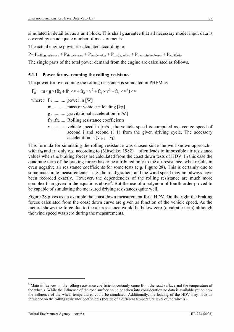
Emission Functions for Heavy Duty Vehicles 39
Federal Environment Agency – Austria BE-223 (2003)
simulated in detail but as a unit block. This shall guarantee that all necessary model input data is covered by an adequate number of measurements.
The actual engine power is calculated according to:
P= Prolling resistance + Pair resistance + Pacceleration + Proad gradient + Ptransmission losses + Pauxiliaries
The single parts of the total power demand from the engine are calculated as follows.
5.1.1 Power for overcoming the rolling resistance
The power for overcoming the rolling resistance is simulated in PHEM as
v)vfrvfrvfrvfr(frgmP 44
33
2210R
where: PR ........... power in [W]
m ............ mass of vehicle + loading [kg]
g ............. gravitational acceleration [m/s2]
fr0..fr4 ..... Rolling resistance coefficients
v ............. vehicle speed in [m/s], the vehicle speed is computed as average speed of second i and second (i+1) from the given driving cycle. The accessory acceleration is (v i+1 – vi).
This formula for simulating the rolling resistance was chosen since the well known approach - with fr0 and fr1 only e.g. according to (Mitschke, 1982) – often leads to impossible air resistance values when the braking forces are calculated from the coast down tests of HDV. In this case the quadratic term of the braking forces has to be attributed only to the air resistance, what results in even negative air resistance coefficients for some tests (e.g. Figure 28). This is certainly due to some inaccurate measurements – e.g. the road gradient and the wind speed may not always have been recorded exactly. However, the dependencies of the rolling resistance are much more complex than given in the equations above2. But the use of a polynom of fourth order proved to be capable of simulating the measured driving resistances quite well.
Figure 28 gives as an example the coast down measurement for a HDV. On the right the braking forces calculated from the coast down curve are given as function of the vehicle speed. As the picture shows the force due to the air resistance would be below zero (quadratic term) although the wind speed was zero during the measurements.
2 Main influences on the rolling resistance coefficients certainly come from the road surface and the temperature of the wheels. While the influence of the road surface could be taken into consideration no data is available yet on how the influence of the wheel temperatures could be simulated. Additionally, the loading of the HDV may have an influence on the rolling resistance coefficients (beside of a different temperature level of the wheels).
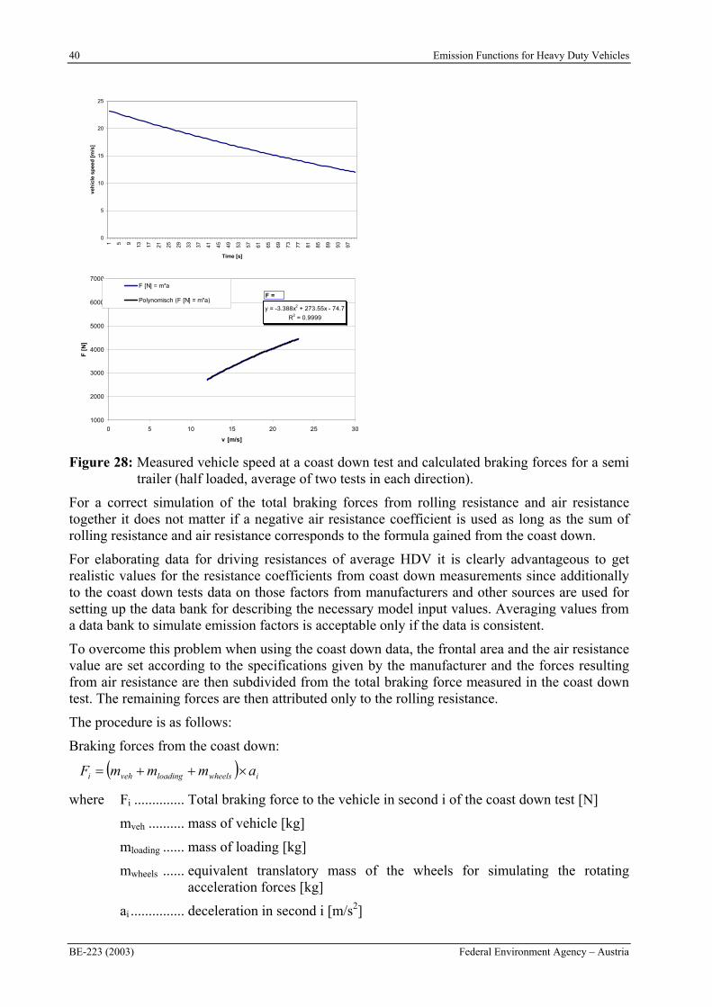
40 Emission Functions for Heavy Duty Vehicles
BE-223 (2003) Federal Environment Agency – Austria
0
5
10
15
20
251 5 9 13 17 21 25 29 33 37 41 45 49 53 57 61 65 69 73 77 81 85 89 93 97
Time [s]
veh
icle
sp
eed
[m
/s]
y = -3.388x2 + 273.55x - 74.7
R2 = 0.9999
1000
2000
3000
4000
5000
6000
7000
0 5 10 15 20 25 30
v [m/s]
F [
N]
F [N] = m*a
Polynomisch (F [N] = m*a)F =
Figure 28: Measured vehicle speed at a coast down test and calculated braking forces for a semi trailer (half loaded, average of two tests in each direction).
For a correct simulation of the total braking forces from rolling resistance and air resistance together it does not matter if a negative air resistance coefficient is used as long as the sum of rolling resistance and air resistance corresponds to the formula gained from the coast down.
For elaborating data for driving resistances of average HDV it is clearly advantageous to get realistic values for the resistance coefficients from coast down measurements since additionally to the coast down tests data on those factors from manufacturers and other sources are used for setting up the data bank for describing the necessary model input values. Averaging values from a data bank to simulate emission factors is acceptable only if the data is consistent.
To overcome this problem when using the coast down data, the frontal area and the air resistance value are set according to the specifications given by the manufacturer and the forces resulting from air resistance are then subdivided from the total braking force measured in the coast down test. The remaining forces are then attributed only to the rolling resistance.
The procedure is as follows:
Braking forces from the coast down:
iwheelsloadingvehi ammmF
where Fi .............. Total braking force to the vehicle in second i of the coast down test [N]
mveh .......... mass of vehicle [kg]
mloading ...... mass of loading [kg]
mwheels ...... equivalent translatory mass of the wheels for simulating the rotating acceleration forces [kg]
ai ............... deceleration in second i [m/s2]
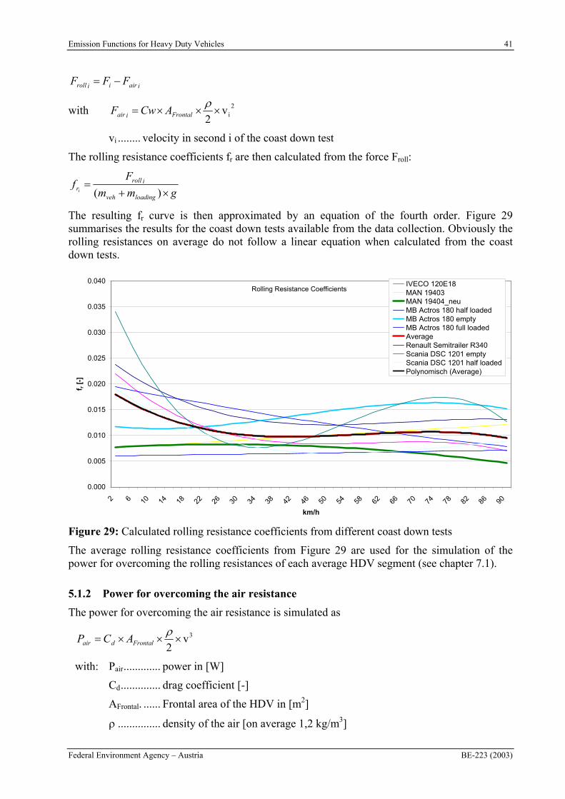
Emission Functions for Heavy Duty Vehicles 41
Federal Environment Agency – Austria BE-223 (2003)
iairiiroll FFF
with 2iv
2Frontaliair ACwF
vi ........ velocity in second i of the coast down test
The rolling resistance coefficients fr are then calculated from the force Froll:
gmm
Ff
loadingveh
irollri )(
The resulting fr curve is then approximated by an equation of the fourth order. Figure 29 summarises the results for the coast down tests available from the data collection. Obviously the rolling resistances on average do not follow a linear equation when calculated from the coast down tests.
Rolling Resistance Coefficients
0.000
0.005
0.010
0.015
0.020
0.025
0.030
0.035
0.040
2 6 10 14 18 22 26 30 34 38 42 46 50 54 58 62 66 70 74 78 82 86 90
km/h
f r [
-]
IVECO 120E18MAN 19403MAN 19404_neuMB Actros 180 half loadedMB Actros 180 emptyMB Actros 180 full loadedAverageRenault Semitrailer R340Scania DSC 1201 emptyScania DSC 1201 half loadedPolynomisch (Average)
Figure 29: Calculated rolling resistance coefficients from different coast down tests
The average rolling resistance coefficients from Figure 29 are used for the simulation of the power for overcoming the rolling resistances of each average HDV segment (see chapter 7.1).
5.1.2 Power for overcoming the air resistance
The power for overcoming the air resistance is simulated as
3v2Frontaldair ACP
with: Pair............. power in [W]
Cd.............. drag coefficient [-]
AFrontal. ...... Frontal area of the HDV in [m2]
............... density of the air [on average 1,2 kg/m3]
42 Emission Functions for Heavy Duty Vehicles
BE-223 (2003) Federal Environment Agency – Austria
As described before, Cd and Afrontal are taken from the specifications given by the manufacturer. If no manufacturer specifications for the Cd value were available the Cd was set according to those of a similar HDV in a data bank of the Institute.
5.1.3 Power for acceleration
The model offers two options for the simulation of the power demand for vehicle acceleration. The more detailed option simulates the rotating masses as three blocks: wheels, gearbox, other rotating masses:
Option 1:
For the calculation the power for the acceleration of the rotating masses is converted to the vehicle acceleration. This gives the following equation:
va)( loadingrotvehiclea mmmP
with: mrot..... to the wheel reduced mass for rotational accelerated parts 22
2wheel
axleontransmissi
wheel
gearaxlemot
wheel
wheelsrot r
iI
r
iiI
r
Im
I ......... moment of inertia from the rotating masses [kg m2]
v......... vehicle speed [m/s]
The part of the wheels can be simplified assuming the wheels to be cylinders (I= m*r2/2)
wheels2m0.5
wheel
wheels
r
I
with: mwheels ..... mass of the vehicles wheels (including rims)
If the moments of inertia are not known, a simplified method is used:
Option 2:
mrot from the formula above is assessed by a “rotating-mass-factor” :
veh
rotveh
m
mm)v(
With this simplification the power for acceleration is:
va))v(( loadingveha mmP
is expressed as function of the vehicle speed in this option to take the influence of the differing transmission ratios and the resulting decreasing influence of angular acceleration of the engine and the gear box block with increasing vehicle speed into consideration.
with: )0667,0*vlog(4,01833,0)v( 0 for 1m/s< v <12m/s
below 1m/s v is set equal 1, above 12m/s v is set to constant 12,0
a................ acceleration of the vehicle [m/s2]
mvehicle....... mass of the vehicle (ready for driving) in [kg]
mloading ...... mass of the payload or the passengers and luggage in [kg]
0 ............. Rotating mass factor, to be given as model input (ca. 1,05 to 1,2)
Emission Functions for Heavy Duty Vehicles 43
Federal Environment Agency – Austria BE-223 (2003)
The formula for option 2 is derived from the more detailed simulation according to the model for option 1.
For the first assessment of the actual power demand always the simplified equation is used since the gear choice of the driver is modelled as a function of the actual power demand. Thus the gear and the transmission ratios are not known at the first step of iteration.
5.1.4 Power for overcoming road gradients
The power for overcoming road gradients is calculated as:
v0,01GradientgmPg
with: Pg .................power in [W]
Gradient.......Road gradient in %
m..................mass of the vehicle + loading in [kg]
The road gradient has to be given as model input value in the file containing the driving cycle on second per second basis.
5.1.5 Power demand of auxiliaries
A more detailed assessment of the power demand from different auxiliaries is planned within the COST 346 project. For the D.A.CH project no detailed data is available for simulating single auxiliaries. The assessment of the HDV measurements on the chassis dynamometer suggested a rather constant power demand of auxiliaries from the tested vehicles (chapter 5.5.3). Thus the power demand is calculated in a simplified way:
rated0sauxiliarie PPP
with: Pauxiliaries..........power in [kW]
P0 ...................power demand of the auxiliaries as ratio to the rated power [-]
For average HDV this equation is sufficient from today’s point of view. For special HDV (garbage trucks, air conditioned HDV bodies, eventually for city buses) a more detailed approach may improve the model accuracy.
5.1.6 Power demand of the transmission system
The power losses between the engine and the wheels are simulated as a function of the actual power, the engine speed and the transmission ratio. A simplified equation according to (Tieber, 1997) – based on transmission efficiencies -is used for a first iteration since the gear choice of the driver is modelled as a function of the actual power demand. Thus the gear and the transmission ratios are not known at the first step of iteration.
The transmission efficiency is defined here as:
Pe
PPe
Pe
P ontransmissidrntransmisso
and dreontransmissi PPP
44 Emission Functions for Heavy Duty Vehicles
BE-223 (2003) Federal Environment Agency – Austria
Simplified equation for the first assessment:
0,57P
P2,7
P
P6
rated
dr
2
rated
drntransmisso where Pdr/Prated <0,2
0,8507P
P0,1182
P
P0,0561
rated
dr
2
rated
drontransmissi where Pdr/Prated >0,2
The power losses in the transmission system are:
drontransmissi
drontransmissi P
PP
with Pdr ...........Power to overcome the driving resistances (without transmission losses)
After the first rough assessment of the power losses in the transmission system (and after the first iteration of the power necessary for the acceleration of rotating masses the next subroutine of PHEM is executed which selects the actual gear by a driver gear-shift model (chapter 5.2).
After the actual gear is found, the losses in the transmission system are simulated according to the following method.
(a) Manual Gear box
The losses in the transmission system are directly calculated as power loss. The use of transmission efficiencies is avoided since the transmission efficiency is near to zero in ranges of low power transmission. This would lead to a not well defined value since a low value for the engine power has to be divided by an efficiency near to zero.
Following the basic method of PHEM, the formulas used are normalised to the rated power of the engine.
Power losses in the Differential [kW]:
rated
dr
rated
wheelratedalDifferenti P
PABS9,53
n
n8,340,47(0,0025PP
with: Prated rated power of the engine
nwheel rotational speed of the wheels [rpm].........lD
v60n
wheelwheel
Pdr Power demand from the engine to overcome the driving resistances (= total power demand without transmission losses)
Power losses in the gear box [kW]:
These losses are simulated for four transmission ratios. The losses for gears between these ratios are interpolated linearly. This method takes the characteristics from splitter-gear shifts – which are most common in HDV – into consideration and was gained from measured data of a gear box.
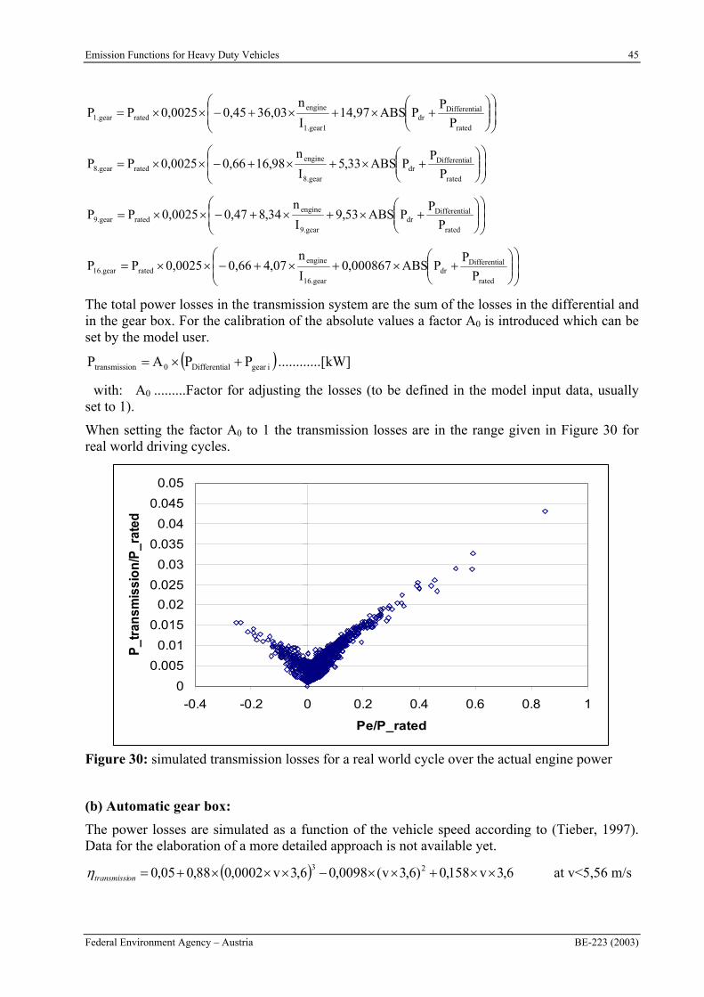
Emission Functions for Heavy Duty Vehicles 45
Federal Environment Agency – Austria BE-223 (2003)
rated
alDifferentidr
1.gear1
enginerated1.gear P
PPABS14,97
I
n36,030,450,0025PP
rated
alDifferentidr
8.gear
enginerated8.gear P
PPABS33,5
I
n98,610,660,0025PP
rated
alDifferentidr
9.gear
enginerated9.gear P
PPABS53,9
I
n34,80,470,0025PP
rated
alDifferentidr
16.gear
enginerated16.gear P
PPABS000867,0
I
n07,40,660,0025PP
The total power losses in the transmission system are the sum of the losses in the differential and in the gear box. For the calibration of the absolute values a factor A0 is introduced which can be set by the model user.
igearalDifferenti0ontransmissi PPAP ............[kW]
with: A0 .........Factor for adjusting the losses (to be defined in the model input data, usually set to 1).
When setting the factor A0 to 1 the transmission losses are in the range given in Figure 30 for real world driving cycles.
0
0.005
0.01
0.015
0.02
0.025
0.03
0.035
0.04
0.045
0.05
-0.4 -0.2 0 0.2 0.4 0.6 0.8 1
Pe/P_rated
P_t
ran
smis
sio
n/P
_rat
ed
Figure 30: simulated transmission losses for a real world cycle over the actual engine power
(b) Automatic gear box:
The power losses are simulated as a function of the vehicle speed according to (Tieber, 1997). Data for the elaboration of a more detailed approach is not available yet.
6,3v158,0)6,3v(0098,06,3v0002,088,005,0 23ontransmissi at v<5,56 m/s
46 Emission Functions for Heavy Duty Vehicles
BE-223 (2003) Federal Environment Agency – Austria
88,0ontransmissi at v>5,56 m/s
The power losses in the transmission system are thus:
drontransmissi
drontransmissi P
PP
With Pdr ...........Power to overcome the driving resistances (without transmission losses)
With the equations given in this chapter the power demand from the engine can be simulated for any vehicle / loading / driving cycle combination.
5.2 Simulation of the engine speed
The actual engine speed depends on the vehicle speed, the wheel diameter and the transmission ratio of the axis and the gear box.
Calculation of the engine speed
wheelgearaxle D
1ii60vn
with: n ............... engine speed [rpm]
v ............... vehicle speed in [m/s]
iaxle ............ transmission ratio of the axle [-]
igear............ transmission ratio of the actual gear [-]
Dwheel ........ Wheel diameter [m]
The main problem for the simulation is the assessment of the actual gear since a given vehicle speed can be driven with different gears and the choice which gear to take is depending on a subjective assessment of the driver.
The gear shift behaviour is modelled in PHEM for different types of drivers:
a) Fast driver,
b) Economic driver,
c) Average driver.
The basic assumption is that the „fast driver” style is located in an rpm range where high engine torque and high engine power are available and that the “economic driver” style is located in an rpm range where the specific fuel consumption is the lowest for the given engine power demand. For these driving styles limits of the engine speed are defined where the gear has to be changed upwards or downwards.
The “average driver” is a mixture of style a) and style b) depending on the engine power needed within the next seconds. If the virtual “average driver” realizes that he will need a high engine power within the next seconds (e.g. for acceleration or a road gradient) he will take a gear rather according to style a), if the coming power demand is rather low he will behave like style b).
The user of the model PHEM can choose any mixtures of style a) to c).
General rules:
1) Independent of the driving style chosen the model checks for every second whether the actual needed engine power is below the given full load curve. If the full load curve is
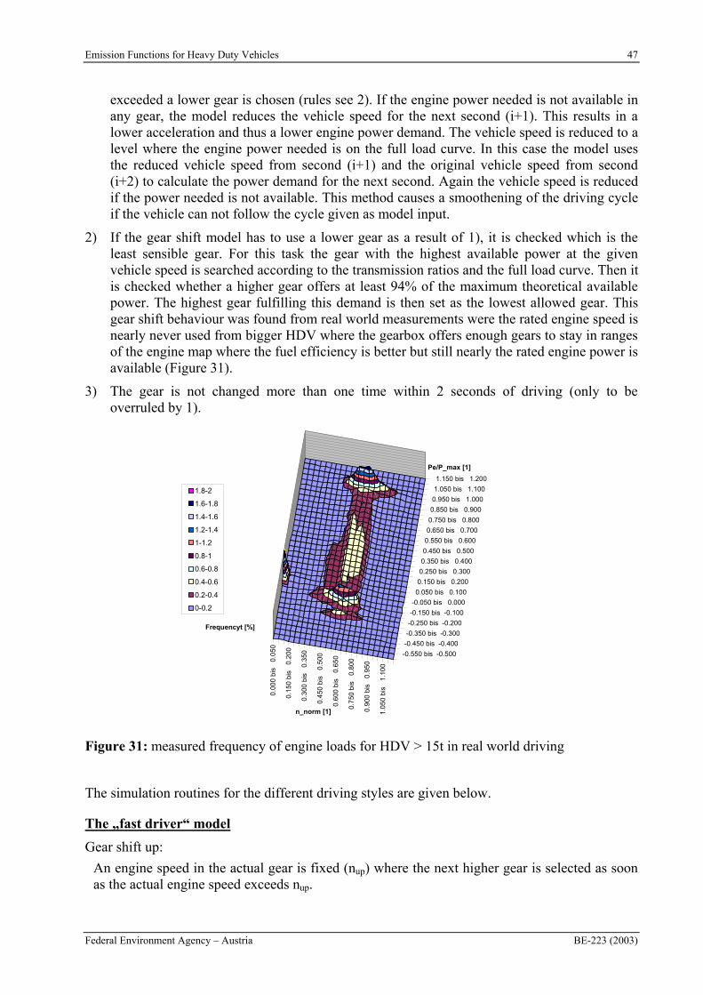
Emission Functions for Heavy Duty Vehicles 47
Federal Environment Agency – Austria BE-223 (2003)
exceeded a lower gear is chosen (rules see 2). If the engine power needed is not available in any gear, the model reduces the vehicle speed for the next second (i+1). This results in a lower acceleration and thus a lower engine power demand. The vehicle speed is reduced to a level where the engine power needed is on the full load curve. In this case the model uses the reduced vehicle speed from second (i+1) and the original vehicle speed from second (i+2) to calculate the power demand for the next second. Again the vehicle speed is reduced if the power needed is not available. This method causes a smoothening of the driving cycle if the vehicle can not follow the cycle given as model input.
2) If the gear shift model has to use a lower gear as a result of 1), it is checked which is the least sensible gear. For this task the gear with the highest available power at the given vehicle speed is searched according to the transmission ratios and the full load curve. Then it is checked whether a higher gear offers at least 94% of the maximum theoretical available power. The highest gear fulfilling this demand is then set as the lowest allowed gear. This gear shift behaviour was found from real world measurements were the rated engine speed is nearly never used from bigger HDV where the gearbox offers enough gears to stay in ranges of the engine map where the fuel efficiency is better but still nearly the rated engine power is available (Figure 31).
3) The gear is not changed more than one time within 2 seconds of driving (only to be overruled by 1).
0.0
00 b
is
0.05
0
0.1
50 b
is
0.20
0
0.3
00 b
is
0.35
0
0.4
50 b
is
0.50
0
0.6
00 b
is
0.65
0
0.7
50 b
is
0.80
0
0.9
00 b
is
0.95
0
1.0
50 b
is
1.10
0
1.150 bis 1.200
1.050 bis 1.100
0.950 bis 1.000
0.850 bis 0.900
0.750 bis 0.800
0.650 bis 0.700
0.550 bis 0.600
0.450 bis 0.500
0.350 bis 0.400
0.250 bis 0.300
0.150 bis 0.200
0.050 bis 0.100
-0.050 bis 0.000
-0.150 bis -0.100
-0.250 bis -0.200
-0.350 bis -0.300
-0.450 bis -0.400
-0.550 bis -0.500
Frequencyt [%]
n_norm [1]
Pe/P_max [1]
1.8-2
1.6-1.8
1.4-1.6
1.2-1.4
1-1.2
0.8-1
0.6-0.8
0.4-0.6
0.2-0.4
0-0.2
Figure 31: measured frequency of engine loads for HDV > 15t in real world driving
The simulation routines for the different driving styles are given below.
The „fast driver“ model
Gear shift up:
An engine speed in the actual gear is fixed (nup) where the next higher gear is selected as soon as the actual engine speed exceeds nup.
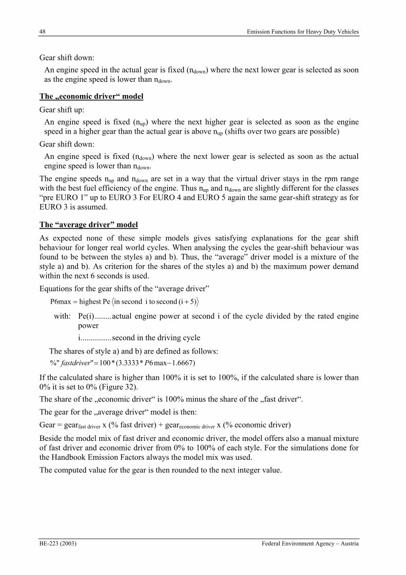
48 Emission Functions for Heavy Duty Vehicles
BE-223 (2003) Federal Environment Agency – Austria
Gear shift down:
An engine speed in the actual gear is fixed (ndown) where the next lower gear is selected as soon as the engine speed is lower than ndown.
The „economic driver“ model
Gear shift up:
An engine speed is fixed (nup) where the next higher gear is selected as soon as the engine speed in a higher gear than the actual gear is above nup (shifts over two gears are possible)
Gear shift down:
An engine speed is fixed (ndown) where the next lower gear is selected as soon as the actual engine speed is lower than ndown.
The engine speeds nup and ndown are set in a way that the virtual driver stays in the rpm range with the best fuel efficiency of the engine. Thus nup and ndown are slightly different for the classes “pre EURO 1” up to EURO 3 For EURO 4 and EURO 5 again the same gear-shift strategy as for EURO 3 is assumed.
The “average driver” model
As expected none of these simple models gives satisfying explanations for the gear shift behaviour for longer real world cycles. When analysing the cycles the gear-shift behaviour was found to be between the styles a) and b). Thus, the “average” driver model is a mixture of the style a) and b). As criterion for the shares of the styles a) and b) the maximum power demand within the next 6 seconds is used.
Equations for the gear shifts of the “average driver”
5)(isecond toisecondinPehighestP6max
with: Pe(i) ........actual engine power at second i of the cycle divided by the rated engine power
i...............second in the driving cycle
The shares of style a) and b) are defined as follows:
)6667.1max6*3333.3(*100"%" Pfastdriver
If the calculated share is higher than 100% it is set to 100%, if the calculated share is lower than 0% it is set to 0% (Figure 32).
The share of the „economic driver“ is 100% minus the share of the „fast driver“.
The gear for the „average driver“ model is then:
Gear = gearfast driver x (% fast driver) + geareconomic driver x (% economic driver)
Beside the model mix of fast driver and economic driver, the model offers also a manual mixture of fast driver and economic driver from 0% to 100% of each style. For the simulations done for the Handbook Emission Factors always the model mix was used.
The computed value for the gear is then rounded to the next integer value.
Emission Functions for Heavy Duty Vehicles 49
Federal Environment Agency – Austria BE-223 (2003)
0%
10%
20%
30%
40%
50%
60%
70%
80%
90%
100%
0% 5% 10%
15%
20%
25%
30%
35%
40%
45%
50%
55%
60%
65%
70%
75%
80%
85%
90%
95%
100%
P_6_max [% from rated power]
sh
are
of
"fa
st
dri
ve
r m
od
el"
Figure 32: share of the “fast driver model” in the “average driver model” as a function of the highest engine power demand within the next 6 seconds
Certainly also this model approach can not simulate all gear changes – especially for single drivers – exactly. But the calculated engine load (rpm and kW combinations) do match the real world driving very well (chapter 7.2). This is the most relevant criterion when interpolating emission factors from an engine map.
As alternative for the simulation of the engine speed the model allows also to set the measured engine speed or the measured gear positions as input variables. In this case the measured values are used instead of the simulated ones. This option is helpful for validation work with measurements from the chassis dynamometer.
5.3 Interpolation from the engine emission map
With the equations given in chapter 5.1 and 5.2 the actual engine speed and the actual engine power are calculated for every second of the driving cycle. With this data the emission values are interpolated from the engine emission maps for every second of the cycle.
The resulting emission values are defined here as “quasi stationary emissions” since they are calculated from an emission map which has been measured under steady state conditions for each point. The total “quasi stationary emissions” over the driving cycle are the integral of the second per second values over the cycle.
The model PHEM is able to handle almost any formats of engine maps concerning the number of points given and according to the content of the maps (emission values, voltages, etc.) if the units are adapted to the model standards (chapter 5.3.2). This flexibility can be used e.g. for the simulation of temperature levels etc.
The routine for the interpolation is described below.
5.3.1 The interpolation routine
For the interpolation multiple options were tested on their accuracy and stability for the given task. The method according to Shepard proved to be the most stable routine for differing layouts of the engine map. With some small adaptations this method proved to be one of the most
50 Emission Functions for Heavy Duty Vehicles
BE-223 (2003) Federal Environment Agency – Austria
accurate interpolation routines for the given task with the additional advantage of a very simple programming.
The adapted Shepard method:
Step 1: the distances between the point to be interpolated and the given points from the engine map in the engine power / engine speed plane are calculated as R2.
2map
2mape
2 )(nn)(PP(i)R ii
with: Pe .............. actual engine power of the point to be interpolated subdivided by the rated power
n................ actual normalised engine speed of the point to be interpolated
Pmap(i) ....... engine power of a point i in the engine map subdivided by the rated power
nmap(i) ....... normalised engine speed of a point i in the engine map
R2 is used also as weighting factor for interpolating points with an engine power >0.05 from rated power.
Step 2: Selection of the points to be used for the interpolation:
Points with R2 < 0,07 are used.
If less than 3 points from the map are within this criterion the radius is doubled until three or more points are within the given radius R2
3.
Step 3: Modified interpolation according to Shepard:
The emission value for the point to be interpolated is simply gained by the weighted average of the points selected in step 2. The weighting is done according to R2 from step 1.
2)(
)(2)(
n),(P 1
1
Eoe
i
imap
i
R
ER
Eo(Pe,n) ............basic interpolated value (emission, fuel consumption, etc.)
Emap-(i) ............value for the point i given in the engine map (points within R2 < 0.07 only)
Since the basic Shepard routine is not capable of making extrapolations the basic interpolated value from the equation above is adjusted assuming a constant emission value [g/kWh] for this small adjustment.
)P(PEoEoE Shen),(Pn),(Pn),(P eee only if Pe greater 0.05
with: E(Pe,n) ....... interpolated value (emission, fuel consumption, etc.)
PSh...........basic interpolated normalised engine power like for Eo(Pe,n)
3 This is not relevant when using the standard formats for the engine maps according to chapter 5.3.2 since the format ensures a sufficient number of points to be located within R2 in any case.
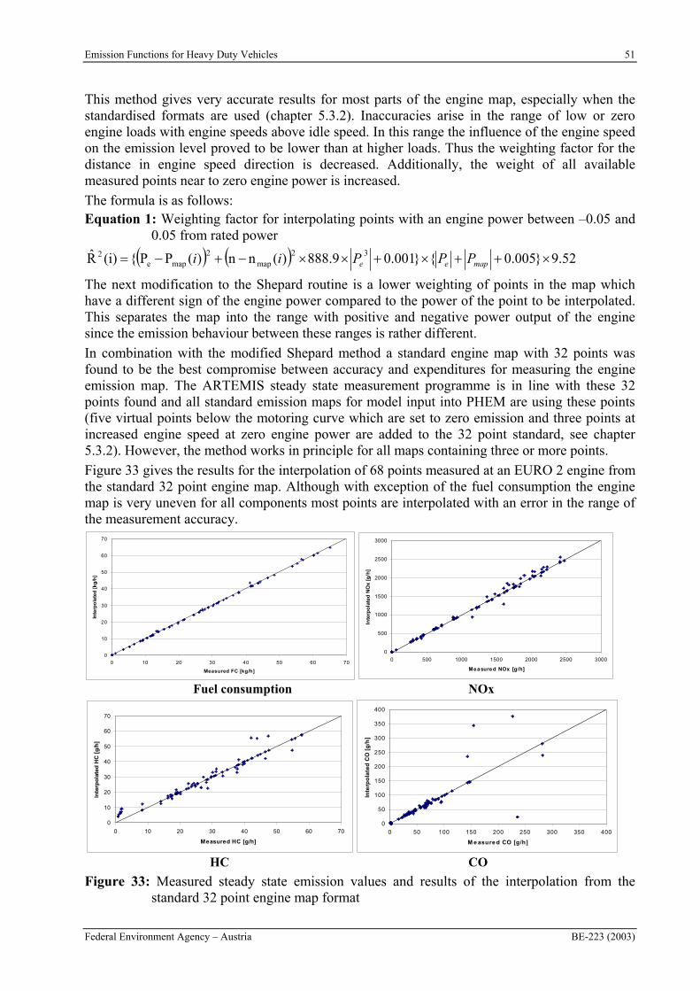
Emission Functions for Heavy Duty Vehicles 51
Federal Environment Agency – Austria BE-223 (2003)
This method gives very accurate results for most parts of the engine map, especially when the standardised formats are used (chapter 5.3.2). Inaccuracies arise in the range of low or zero engine loads with engine speeds above idle speed. In this range the influence of the engine speed on the emission level proved to be lower than at higher loads. Thus the weighting factor for the distance in engine speed direction is decreased. Additionally, the weight of all available measured points near to zero engine power is increased.
The formula is as follows: Equation 1: Weighting factor for interpolating points with an engine power between –0.05 and
0.05 from rated power
52.9}005.0{}001.09.888)(nn)(PP{(i)R̂ 32map
2mape
2mapee PPPii
The next modification to the Shepard routine is a lower weighting of points in the map which have a different sign of the engine power compared to the power of the point to be interpolated. This separates the map into the range with positive and negative power output of the engine since the emission behaviour between these ranges is rather different.
In combination with the modified Shepard method a standard engine map with 32 points was found to be the best compromise between accuracy and expenditures for measuring the engine emission map. The ARTEMIS steady state measurement programme is in line with these 32 points found and all standard emission maps for model input into PHEM are using these points (five virtual points below the motoring curve which are set to zero emission and three points at increased engine speed at zero engine power are added to the 32 point standard, see chapter 5.3.2). However, the method works in principle for all maps containing three or more points.
Figure 33 gives the results for the interpolation of 68 points measured at an EURO 2 engine from the standard 32 point engine map. Although with exception of the fuel consumption the engine map is very uneven for all components most points are interpolated with an error in the range of the measurement accuracy.
0
10
20
30
40
50
60
70
0 10 20 30 40 50 60 70
Measured FC [kg/h]
Inte
rpo
late
d [
kg
/h]
0
500
1000
1500
2000
2500
3000
0 500 1000 1500 2000 2500 3000
Measured NOx [g/h]
Inte
rpo
late
d N
Ox
[g/h
]
Fuel consumption NOx
0
10
20
30
40
50
60
70
0 10 20 30 40 50 60 70
Measured HC [g/h]
Inte
rpo
late
d H
C [
g/h
]
0
50
100
150
200
250
300
350
400
0 50 100 150 200 250 300 350 400
M e asure d CO [g/h]
Inte
rpo
late
d C
O [
g/h
]
HC CO
Figure 33: Measured steady state emission values and results of the interpolation from the standard 32 point engine map format
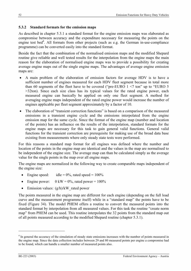
52 Emission Functions for Heavy Duty Vehicles
BE-223 (2003) Federal Environment Agency – Austria
5.3.2 Standard formats for the emission maps
As described in chapter 5.3.1 a standard format for the engine emission maps was elaborated as compromise between accuracy and the expenditure necessary for measuring the points on the engine test bed4. All formats from other projects (such as e.g. the German in-use-compliance programme) can be converted easily into the standard format.
Beside the fact that the combination of the normalised emission maps and the modified Shepard routine give reliable and well tested results for the interpolation from the engine maps the main reason for the elaboration of normalised engine maps was to provide a possibility for creating average engine maps out of the single engine maps. The advantages of average engine emission maps are:
A main problem of the elaboration of emission factors for average HDV is to have a sufficient number of engines measured for each HDV fleet segment because in total more than 60 segments of the fleet have to be covered (“pre-EURO 1 <7 ton” up to “EURO 5 >32ton). Since each size class has its typical values for the rated engine power, each measured engine can basically be applied on only one fleet segment. A method for averaging engine maps independent of the rated engine power would increase the number of engines applicable per fleet segment approximately by a factor of 10.
The elaboration of “transient correction functions” is based on a comparison of the measured emissions in a transient engine cycle and the emissions interpolated from the engine emission map for the same cycle. Since the format of the engine map (number and location of the points) has an influence on the results of the interpolation, standard formats for the engine maps are necessary for this task to gain general valid functions. General valid functions for the transient correction are prerequisite for making use of the broad data base existing from measurements where only steady state tests were performed.
For this reasons a standard map format for all engines was defined where the number and location of the points in the engine map are identical and the values in the map are normalised to be independent of the engine size. The average map can than be calculated simply as the average value for the single points in the map over all engine maps.
The engine maps are normalized in the following way to create comparable maps independent of the engine size:
Engine speed: idle = 0%, rated speed = 100%
Engine power: 0 kW = 0%, rated power = 100%
Emission values: (g/h)/kW_rated power
The points measured in the engine map are different for each engine (depending on the full load curve and the measurement programme itself) while in a “standard map” the points have to be fixed (Figure 34). The model PHEM offers a routine to convert the measured points into the standard format by interpolation from all measured values. For this task the routine “create norm map” from PHEM can be used. This routine interpolates the 32 points from the standard map out of all points measured according to the modified Shepard routine (chapter 5.3.1).
4 In general the accuracy of the simulation of steady state emissions increases with the number of points measured in the engine map. Since the data collection includes between 29 and 80 measured points per engine a compromise had to be found, which can handle a smaller number of measured points also.
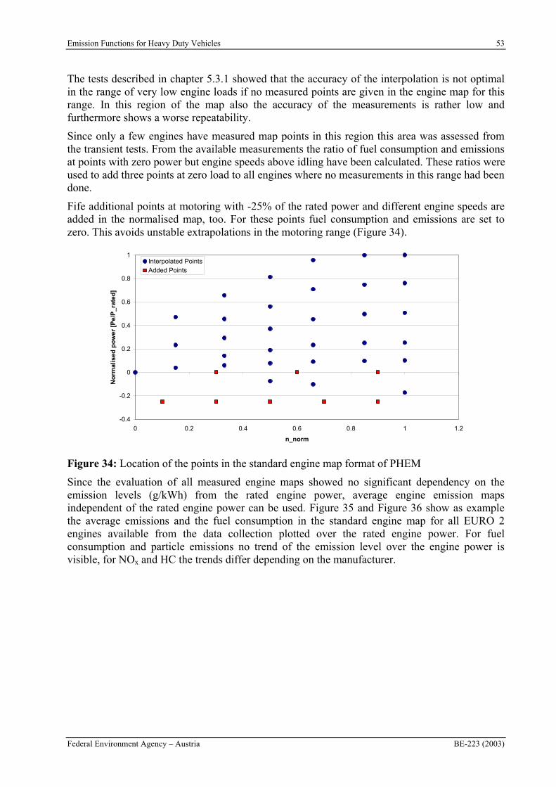
Emission Functions for Heavy Duty Vehicles 53
Federal Environment Agency – Austria BE-223 (2003)
The tests described in chapter 5.3.1 showed that the accuracy of the interpolation is not optimal in the range of very low engine loads if no measured points are given in the engine map for this range. In this region of the map also the accuracy of the measurements is rather low and furthermore shows a worse repeatability.
Since only a few engines have measured map points in this region this area was assessed from the transient tests. From the available measurements the ratio of fuel consumption and emissions at points with zero power but engine speeds above idling have been calculated. These ratios were used to add three points at zero load to all engines where no measurements in this range had been done.
Fife additional points at motoring with -25% of the rated power and different engine speeds are added in the normalised map, too. For these points fuel consumption and emissions are set to zero. This avoids unstable extrapolations in the motoring range (Figure 34).
-0.4
-0.2
0
0.2
0.4
0.6
0.8
1
0 0.2 0.4 0.6 0.8 1 1.2
n_norm
No
rmal
ised
po
wer
[P
e/P
_rat
ed]
Interpolated PointsAdded Points
Figure 34: Location of the points in the standard engine map format of PHEM
Since the evaluation of all measured engine maps showed no significant dependency on the emission levels (g/kWh) from the rated engine power, average engine emission maps independent of the rated engine power can be used. Figure 35 and Figure 36 show as example the average emissions and the fuel consumption in the standard engine map for all EURO 2 engines available from the data collection plotted over the rated engine power. For fuel consumption and particle emissions no trend of the emission level over the engine power is visible, for NOx and HC the trends differ depending on the manufacturer.
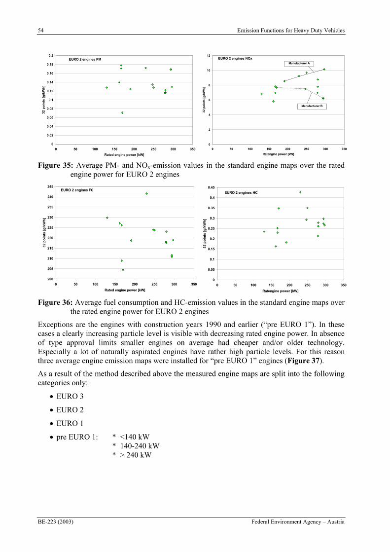
54 Emission Functions for Heavy Duty Vehicles
BE-223 (2003) Federal Environment Agency – Austria
EURO 2 engines NOx
0
2
4
6
8
10
12
0 50 100 150 200 250 300 350
Ratengine power [kW]
32 p
oin
ts [
g/k
Wh
]
Manufacturer B
Manufacturer AEURO 2 engines PM
0
0.02
0.04
0.06
0.08
0.1
0.12
0.14
0.16
0.18
0.2
0 50 100 150 200 250 300 350
Rated engine power [kW]
32
po
ints
[g
/kW
h]
Figure 35: Average PM- and NOx-emission values in the standard engine maps over the rated engine power for EURO 2 engines
EURO 2 engines FC
200
205
210
215
220
225
230
235
240
245
0 50 100 150 200 250 300 350
Rated engine power [kW]
32
po
ints
[g
/kW
h]
EURO 2 engines HC
0
0.05
0.1
0.15
0.2
0.25
0.3
0.35
0.4
0.45
0 50 100 150 200 250 300 350
Ratengine power [kW]
32 p
oin
ts [
g/k
Wh
]
Figure 36: Average fuel consumption and HC-emission values in the standard engine maps over the rated engine power for EURO 2 engines
Exceptions are the engines with construction years 1990 and earlier (“pre EURO 1”). In these cases a clearly increasing particle level is visible with decreasing rated engine power. In absence of type approval limits smaller engines on average had cheaper and/or older technology. Especially a lot of naturally aspirated engines have rather high particle levels. For this reason three average engine emission maps were installed for “pre EURO 1” engines (Figure 37).
As a result of the method described above the measured engine maps are split into the following categories only:
EURO 3
EURO 2
EURO 1
pre EURO 1: * <140 kW * 140-240 kW * > 240 kW
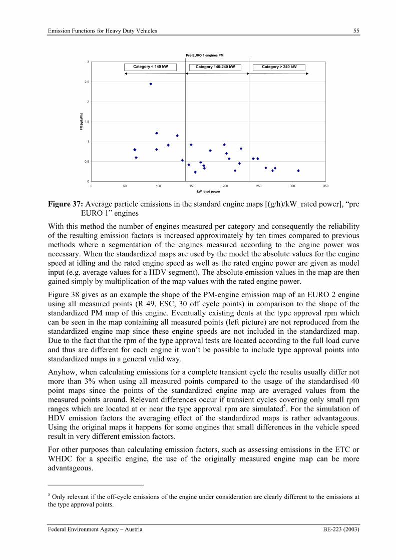
Emission Functions for Heavy Duty Vehicles 55
Federal Environment Agency – Austria BE-223 (2003)
0
0.5
1
1.5
2
2.5
3
0 50 100 150 200 250 300 350
kW rated power
PM
[g
/kW
h]
Category < 140 kW Category > 240 kWCategory 140-240 kW
Pre-EURO 1 engines PM
Figure 37: Average particle emissions in the standard engine maps [(g/h)/kW_rated power], “pre EURO 1” engines
With this method the number of engines measured per category and consequently the reliability of the resulting emission factors is increased approximately by ten times compared to previous methods where a segmentation of the engines measured according to the engine power was necessary. When the standardized maps are used by the model the absolute values for the engine speed at idling and the rated engine speed as well as the rated engine power are given as model input (e.g. average values for a HDV segment). The absolute emission values in the map are then gained simply by multiplication of the map values with the rated engine power.
Figure 38 gives as an example the shape of the PM-engine emission map of an EURO 2 engine using all measured points (R 49, ESC, 30 off cycle points) in comparison to the shape of the standardized PM map of this engine. Eventually existing dents at the type approval rpm which can be seen in the map containing all measured points (left picture) are not reproduced from the standardized engine map since these engine speeds are not included in the standardized map. Due to the fact that the rpm of the type approval tests are located according to the full load curve and thus are different for each engine it won’t be possible to include type approval points into standardized maps in a general valid way.
Anyhow, when calculating emissions for a complete transient cycle the results usually differ not more than 3% when using all measured points compared to the usage of the standardised 40 point maps since the points of the standardized engine map are averaged values from the measured points around. Relevant differences occur if transient cycles covering only small rpm ranges which are located at or near the type approval rpm are simulated5. For the simulation of HDV emission factors the averaging effect of the standardized maps is rather advantageous. Using the original maps it happens for some engines that small differences in the vehicle speed result in very different emission factors.
For other purposes than calculating emission factors, such as assessing emissions in the ETC or WHDC for a specific engine, the use of the originally measured engine map can be more advantageous.
5 Only relevant if the off-cycle emissions of the engine under consideration are clearly different to the emissions at the type approval points.
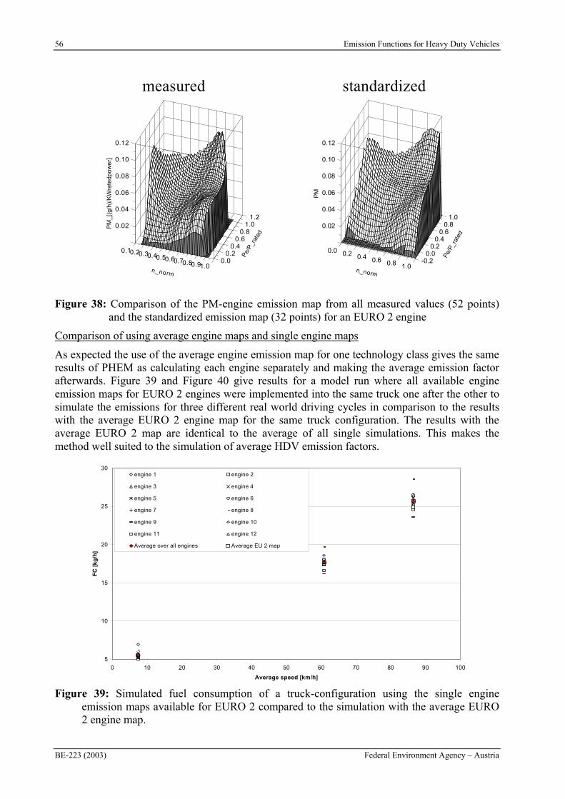
56 Emission Functions for Heavy Duty Vehicles
BE-223 (2003) Federal Environment Agency – Austria
0.10.20.30.40.50.60.70.80.91.0n_norm
0.00.2
0.40.6
0.81.0
1.2
Pe/
P_r
ated
0.02
0.04
0.06
0.08
0.10
0.12
PM
_[(
g/h
)/K
Wra
ted
po
we
r]
0.0 0.2 0.4 0.6 0.8 1.0n_norm
-0.20.0
0.20.4
0.60.8
1.0
Pe/
P_r
ated
0.02
0.04
0.06
0.08
0.10
0.12
PM
measured standardized
Figure 38: Comparison of the PM-engine emission map from all measured values (52 points) and the standardized emission map (32 points) for an EURO 2 engine
Comparison of using average engine maps and single engine maps
As expected the use of the average engine emission map for one technology class gives the same results of PHEM as calculating each engine separately and making the average emission factor afterwards. Figure 39 and Figure 40 give results for a model run where all available engine emission maps for EURO 2 engines were implemented into the same truck one after the other to simulate the emissions for three different real world driving cycles in comparison to the results with the average EURO 2 engine map for the same truck configuration. The results with the average EURO 2 map are identical to the average of all single simulations. This makes the method well suited to the simulation of average HDV emission factors.
5
10
15
20
25
30
0 10 20 30 40 50 60 70 80 90 100
Average speed [km/h]
FC
[kg
/h]
engine 1 engine 2
engine 3 engine 4
engine 5 engine 6
engine 7 engine 8
engine 9 engine 10
engine 11 engine 12
Average over all engines Average EU 2 map
Figure 39: Simulated fuel consumption of a truck-configuration using the single engine emission maps available for EURO 2 compared to the simulation with the average EURO 2 engine map.
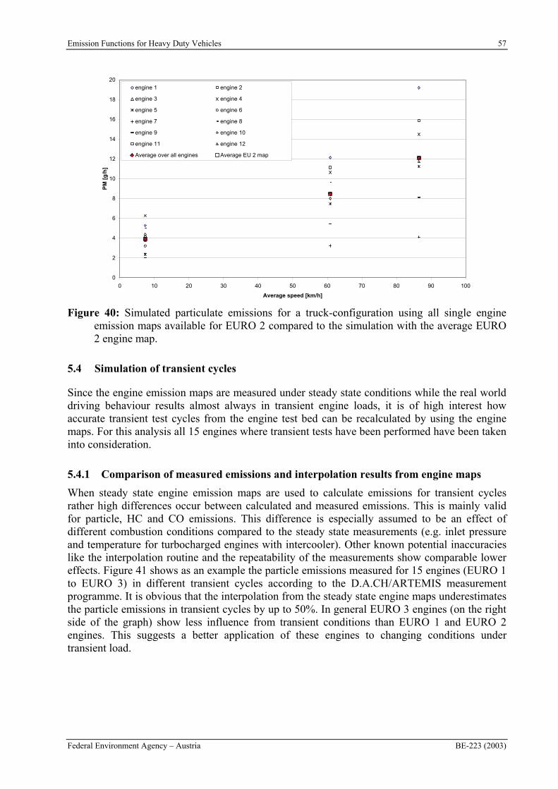
Emission Functions for Heavy Duty Vehicles 57
Federal Environment Agency – Austria BE-223 (2003)
0
2
4
6
8
10
12
14
16
18
20
0 10 20 30 40 50 60 70 80 90 100
Average speed [km/h]
PM
[g
/h]
engine 1 engine 2
engine 3 engine 4
engine 5 engine 6
engine 7 engine 8
engine 9 engine 10
engine 11 engine 12
Average over all engines Average EU 2 map
Figure 40: Simulated particulate emissions for a truck-configuration using all single engine emission maps available for EURO 2 compared to the simulation with the average EURO 2 engine map.
5.4 Simulation of transient cycles
Since the engine emission maps are measured under steady state conditions while the real world driving behaviour results almost always in transient engine loads, it is of high interest how accurate transient test cycles from the engine test bed can be recalculated by using the engine maps. For this analysis all 15 engines where transient tests have been performed have been taken into consideration.
5.4.1 Comparison of measured emissions and interpolation results from engine maps
When steady state engine emission maps are used to calculate emissions for transient cycles rather high differences occur between calculated and measured emissions. This is mainly valid for particle, HC and CO emissions. This difference is especially assumed to be an effect of different combustion conditions compared to the steady state measurements (e.g. inlet pressure and temperature for turbocharged engines with intercooler). Other known potential inaccuracies like the interpolation routine and the repeatability of the measurements show comparable lower effects. Figure 41 shows as an example the particle emissions measured for 15 engines (EURO 1 to EURO 3) in different transient cycles according to the D.A.CH/ARTEMIS measurement programme. It is obvious that the interpolation from the steady state engine maps underestimates the particle emissions in transient cycles by up to 50%. In general EURO 3 engines (on the right side of the graph) show less influence from transient conditions than EURO 1 and EURO 2 engines. This suggests a better application of these engines to changing conditions under transient load.
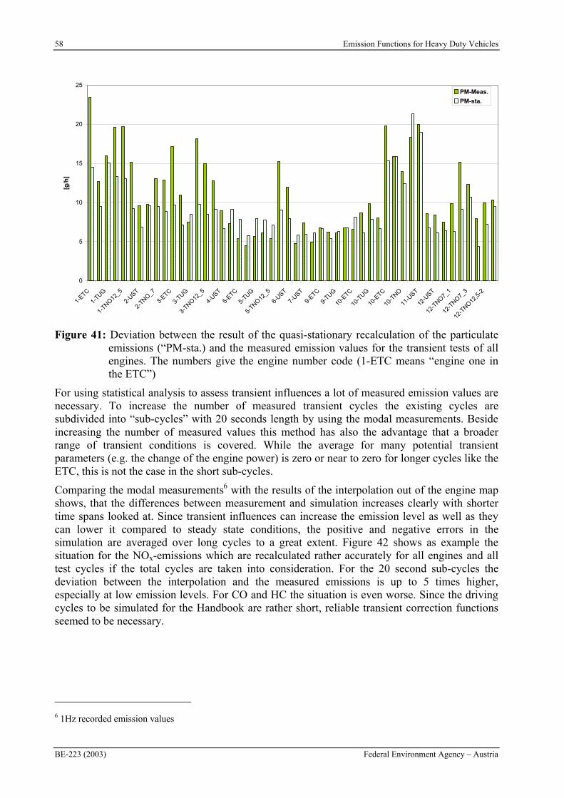
58 Emission Functions for Heavy Duty Vehicles
BE-223 (2003) Federal Environment Agency – Austria
0
5
10
15
20
25
1-ETC
1-TUG
1-TNO12
_5
2-UST
2-TNO_7
3-ETC
3-TUG
3-TNO12
_5
4-UST
5-ETC
5-TUG
5-TNO12
_5
6-UST
7-UST
9-ETC
9-TUG
10-E
TC
10-T
UG
10-E
TC
10-T
NO
11-U
ST
12-U
ST
12-T
NO7_1
12-T
NO7_3
12-T
NO12,5
-2
[g/h
]
PM-Meas.
PM-sta.
Figure 41: Deviation between the result of the quasi-stationary recalculation of the particulate emissions (“PM-sta.) and the measured emission values for the transient tests of all engines. The numbers give the engine number code (1-ETC means “engine one in the ETC”)
For using statistical analysis to assess transient influences a lot of measured emission values are necessary. To increase the number of measured transient cycles the existing cycles are subdivided into “sub-cycles” with 20 seconds length by using the modal measurements. Beside increasing the number of measured values this method has also the advantage that a broader range of transient conditions is covered. While the average for many potential transient parameters (e.g. the change of the engine power) is zero or near to zero for longer cycles like the ETC, this is not the case in the short sub-cycles.
Comparing the modal measurements6 with the results of the interpolation out of the engine map shows, that the differences between measurement and simulation increases clearly with shorter time spans looked at. Since transient influences can increase the emission level as well as they can lower it compared to steady state conditions, the positive and negative errors in the simulation are averaged over long cycles to a great extent. Figure 42 shows as example the situation for the NOx-emissions which are recalculated rather accurately for all engines and all test cycles if the total cycles are taken into consideration. For the 20 second sub-cycles the deviation between the interpolation and the measured emissions is up to 5 times higher, especially at low emission levels. For CO and HC the situation is even worse. Since the driving cycles to be simulated for the Handbook are rather short, reliable transient correction functions seemed to be necessary.
6 1Hz recorded emission values
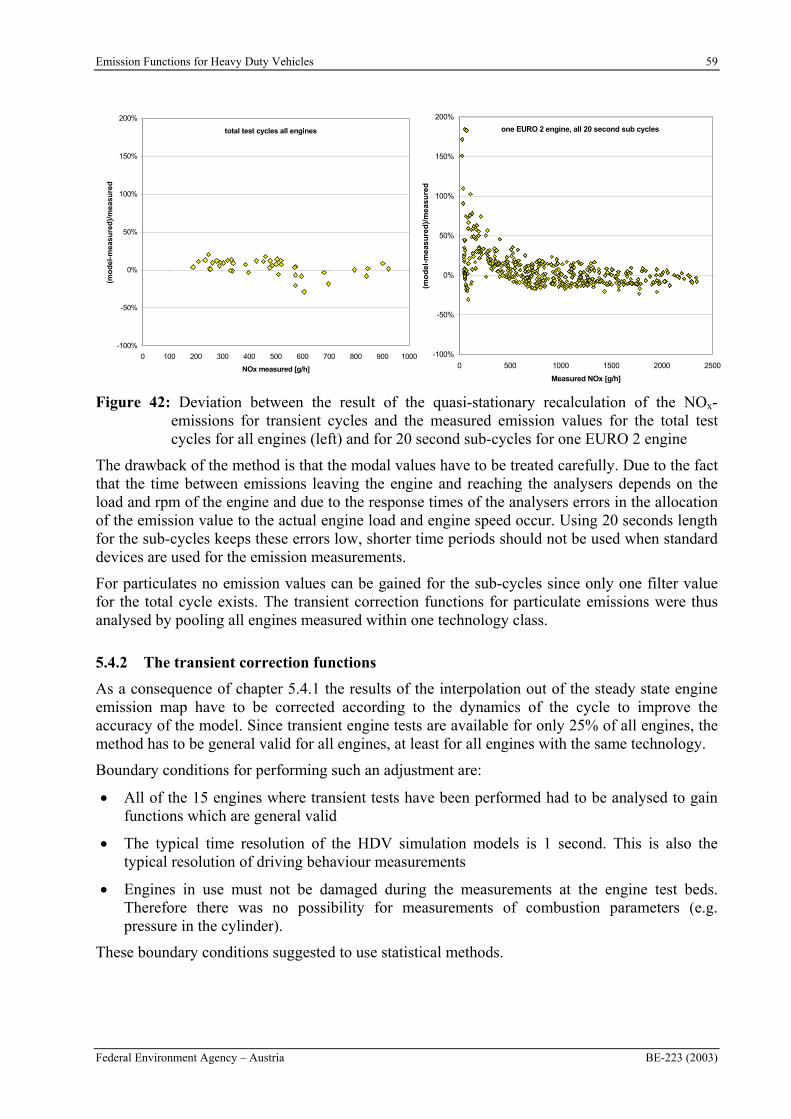
Emission Functions for Heavy Duty Vehicles 59
Federal Environment Agency – Austria BE-223 (2003)
-100%
-50%
0%
50%
100%
150%
200%
0 100 200 300 400 500 600 700 800 900 1000
NOx measured [g/h]
(mo
del
-mea
sure
d)/
mea
sure
d
total test cycles all engines
-100%
-50%
0%
50%
100%
150%
200%
0 500 1000 1500 2000 2500
Measured NOx [g/h]
(mo
del
-mea
sure
d)/
mea
sure
d
one EURO 2 engine, all 20 second sub cycles
Figure 42: Deviation between the result of the quasi-stationary recalculation of the NOx-emissions for transient cycles and the measured emission values for the total test cycles for all engines (left) and for 20 second sub-cycles for one EURO 2 engine
The drawback of the method is that the modal values have to be treated carefully. Due to the fact that the time between emissions leaving the engine and reaching the analysers depends on the load and rpm of the engine and due to the response times of the analysers errors in the allocation of the emission value to the actual engine load and engine speed occur. Using 20 seconds length for the sub-cycles keeps these errors low, shorter time periods should not be used when standard devices are used for the emission measurements.
For particulates no emission values can be gained for the sub-cycles since only one filter value for the total cycle exists. The transient correction functions for particulate emissions were thus analysed by pooling all engines measured within one technology class.
5.4.2 The transient correction functions
As a consequence of chapter 5.4.1 the results of the interpolation out of the steady state engine emission map have to be corrected according to the dynamics of the cycle to improve the accuracy of the model. Since transient engine tests are available for only 25% of all engines, the method has to be general valid for all engines, at least for all engines with the same technology.
Boundary conditions for performing such an adjustment are:
All of the 15 engines where transient tests have been performed had to be analysed to gain functions which are general valid
The typical time resolution of the HDV simulation models is 1 second. This is also the typical resolution of driving behaviour measurements
Engines in use must not be damaged during the measurements at the engine test beds. Therefore there was no possibility for measurements of combustion parameters (e.g. pressure in the cylinder).
These boundary conditions suggested to use statistical methods.
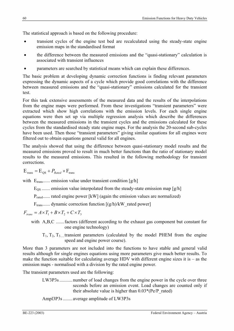
60 Emission Functions for Heavy Duty Vehicles
BE-223 (2003) Federal Environment Agency – Austria
The statistical approach is based on the following procedure:
transient cycles of the engine test bed are recalculated using the steady-state engine emission maps in the standardised format
the difference between the measured emissions and the “quasi-stationary” calculation is associated with transient influences
parameters are searched by statistical means which can explain these differences.
The basic problem at developing dynamic correction functions is finding relevant parameters expressing the dynamic aspects of a cycle which provide good correlations with the difference between measured emissions and the “quasi-stationary” emissions calculated for the transient test.
For this task extensive assessments of the measured data and the results of the interpolations from the engine maps were performed. From these investigations “transient parameters” were extracted which show high correlations with the emission levels. For each single engine equations were then set up via multiple regression analysis which describe the differences between the measured emissions in the transient cycles and the emissions calculated for these cycles from the standardised steady state engine maps. For the analysis the 20-second sub-cycles have been used. Then those “transient parameters” giving similar equations for all engines were filtered out to obtain equations general valid for all engines.
The analysis showed that using the difference between quasi-stationary model results and the measured emissions proved to result in much better functions than the ratio of stationary model results to the measured emissions. This resulted in the following methodology for transient corrections.
transQStrans FEE RatedP
with Etrans...... emission value under transient condition [g/h]
EQS ....... emission value interpolated from the steady-state emission map [g/h]
Prated...... rated engine power [kW] (again the emission values are normalized)
Ftrans...... dynamic correction function [(g/h)/kW_rated power]
321 TCTBTAFtrans
with A,B,C ....... factors (different according to the exhaust gas component but constant for one engine technology)
T1, T2, T3.....transient parameters (calculated by the model PHEM from the engine speed and engine power course).
More than 3 parameters are not included into the functions to have stable and general valid results although for single engines equations using more parameters give much better results. To make the function suitable for calculating average HDV with different engine sizes it is – as the emission maps - normalised with a division by the rated engine power.
The transient parameters used are the following:
LW3P3s ...........number of load changes from the engine power in the cycle over three seconds before an emission event. Load changes are counted only if their absolute value is higher than 0.03*(Pe/P_rated)
Ampl3P3s ........ average amplitude of LW3P3s
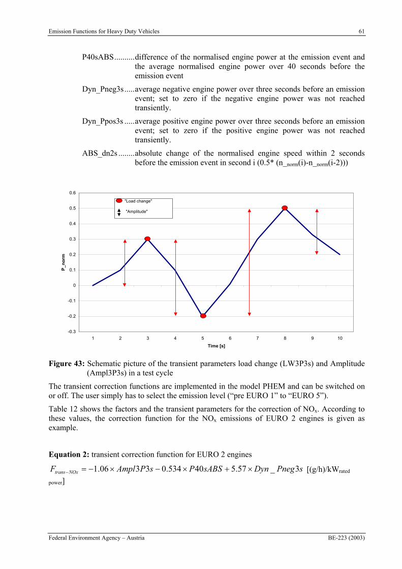
Emission Functions for Heavy Duty Vehicles 61
Federal Environment Agency – Austria BE-223 (2003)
P40sABS..........difference of the normalised engine power at the emission event and the average normalised engine power over 40 seconds before the emission event
Dyn_Pneg3s.....average negative engine power over three seconds before an emission event; set to zero if the negative engine power was not reached transiently.
Dyn_Ppos3s .....average positive engine power over three seconds before an emission event; set to zero if the positive engine power was not reached transiently.
ABS_dn2s ........absolute change of the normalised engine speed within 2 seconds before the emission event in second i (0.5* (n_norm(i)-n_norm(i-2)))
-0.3
-0.2
-0.1
0
0.1
0.2
0.3
0.4
0.5
0.6
1 2 3 4 5 6 7 8 9 10
Time [s]
P_n
orm
"Load change"
"Amplitude"
Figure 43: Schematic picture of the transient parameters load change (LW3P3s) and Amplitude (Ampl3P3s) in a test cycle
The transient correction functions are implemented in the model PHEM and can be switched on or off. The user simply has to select the emission level (“pre EURO 1” to “EURO 5”).
Table 12 shows the factors and the transient parameters for the correction of NOx. According to these values, the correction function for the NOx emissions of EURO 2 engines is given as example.
Equation 2: transient correction function for EURO 2 engines
sPnegDynsABSPsPAmplF NOxtrans 3_57.540534.03306.1 [(g/h)/kWrated
power]
62 Emission Functions for Heavy Duty Vehicles
BE-223 (2003) Federal Environment Agency – Austria
Table 12: Transient factors for the NOx correction
Ampl3P3s P40sABS ABS_dn2s
EURO 0 0.180 -0.290 -1.800
EURO 1 0.151 -0.303 -1.994
EURO 2 0.151 -0.303 -1.994
EURO 3 1.051 -0.289 -1.488
EURO 4 as EURO 3
EURO 5 as EURO 3
HC and CO are corrected in an analogous way. The corresponding transient factors are shown in Table 13.
Table 13: Transient factors for the CO and HC correction
CO HC
Ampl3P3s P40sABS LW3P3s Ampl3P3s LW3P3s Dyn_Pneg3s
EURO 0 3.982 0.375 -0.104 -0.0723 0.002154 -0.121
EURO 1 3.982 0.375 -0.104 -0.0723 0.002154 -0.121
EURO 2 3.982 0.375 -0.104 -0.0723 0.002154 -0.121
EURO 3 3.190 0.238 -0.0908 -0.0413 -0.0228 -0.0283
EURO 4 As EURO 3 As EURO 3
EURO 5 As EURO 3 As EURO 3
Because of the limited number of measured particulate emissions (no sub-cycles possible) it was not possible to elaborate separate functions for the “pre EURO 1” engines, especially for the three engine-power-sub-categories in this class (chapter 5.3.2). The few available transient tests for those engines showed a similar general tendency as the EURO 1 and EURO 2 engines. Thus the same functions are applied (Table 14). Euro 3 engines generally show less increase of the particle emission level under transient cycles compared to steady state tests. This results from a better engine application using inter alia the features provided by modern fuel injection systems and optimised turbo charge systems using variable turbine geometries. The low particle emission limits from EURO 4 on will not allow significant increases under transient conditions compared to steady state operation if the ETC has to be passed. Thus the transient correction functions for EURO 4 and EURO 5 engines were set to zero (chapter 6).
Table 14: Transient factors for the particulate emission correction
Ampl3P3s LW3P3s Dyn_Pneg3s
EURO 0 0.525 -0.0153 0.442
EURO 1 0.525 -0.0153 0.442
EURO 2 0.525 -0.0153 0.442
EURO 3 0.141 -0.0099 -0.584
EURO 4 0 0 0
EURO 5 0 0 0
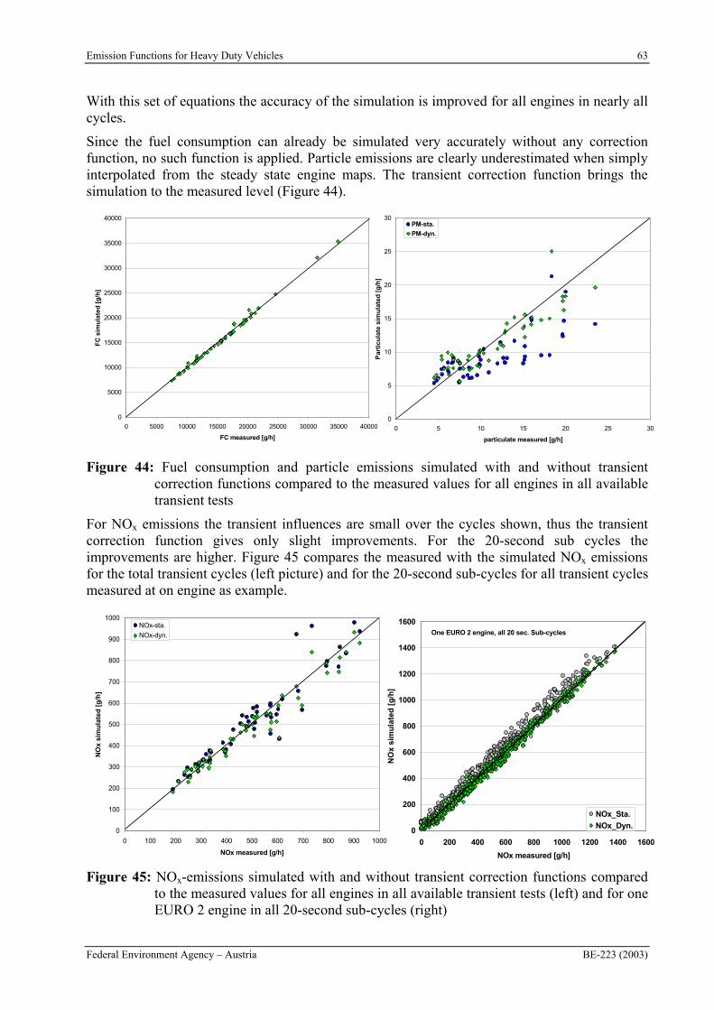
Emission Functions for Heavy Duty Vehicles 63
Federal Environment Agency – Austria BE-223 (2003)
With this set of equations the accuracy of the simulation is improved for all engines in nearly all cycles.
Since the fuel consumption can already be simulated very accurately without any correction function, no such function is applied. Particle emissions are clearly underestimated when simply interpolated from the steady state engine maps. The transient correction function brings the simulation to the measured level (Figure 44).
0
5000
10000
15000
20000
25000
30000
35000
40000
0 5000 10000 15000 20000 25000 30000 35000 40000
FC measured [g/h]
FC
sim
ula
ted
[g
/h]
0
5
10
15
20
25
30
0 5 10 15 20 25 30
particulate measured [g/h]
Par
ticu
late
sim
ula
ted
[g
/h]
PM-sta.
PM-dyn.
Figure 44: Fuel consumption and particle emissions simulated with and without transient correction functions compared to the measured values for all engines in all available transient tests
For NOx emissions the transient influences are small over the cycles shown, thus the transient correction function gives only slight improvements. For the 20-second sub cycles the improvements are higher. Figure 45 compares the measured with the simulated NOx emissions for the total transient cycles (left picture) and for the 20-second sub-cycles for all transient cycles measured at on engine as example.
0
100
200
300
400
500
600
700
800
900
1000
0 100 200 300 400 500 600 700 800 900 1000
NOx measured [g/h]
NO
x si
mu
late
d [
g/h
]
NOx-sta.
NOx-dyn.
0
200
400
600
800
1000
1200
1400
1600
0 200 400 600 800 1000 1200 1400 1600
NOx measured [g/h]
NO
x si
mu
late
d [
g/h
]
NOx_Sta.
NOx_Dyn.
One EURO 2 engine, all 20 sec. Sub-cycles
Figure 45: NOx-emissions simulated with and without transient correction functions compared to the measured values for all engines in all available transient tests (left) and for one EURO 2 engine in all 20-second sub-cycles (right)
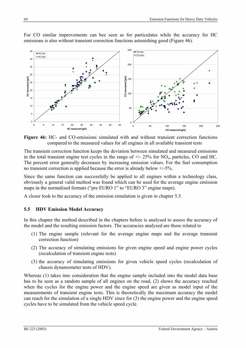
64 Emission Functions for Heavy Duty Vehicles
BE-223 (2003) Federal Environment Agency – Austria
For CO similar improvements can bee seen as for particulates while the accuracy for HC emissions is also without transient correction functions astonishing good (Figure 46).
0
5
10
15
20
25
30
35
40
45
0 5 10 15 20 25 30 35 40 45
HC measured [g/h]
HC
sim
ula
ted
[g
/h]
HC-sta.
HC-dyn.
0
50
100
150
200
250
0 50 100 150 200 250
CO measured [g/h]
CO
sim
ula
ted
[g
/h]
CO-sta.
CO-dyn.
Figure 46: HC- and CO-emissions simulated with and without transient correction functions compared to the measured values for all engines in all available transient tests
The transient correction function keeps the deviation between simulated and measured emissions in the total transient engine test cycles in the range of +/- 25% for NOx, particles, CO and HC. The percent error generally decreases by increasing emission values. For the fuel consumption no transient correction is applied because the error is already below +/-5%.
Since the same function can successfully be applied to all engines within a technology class, obviously a general valid method was found which can be used for the average engine emission maps in the normalised formats (“pre EURO 1” to “EURO 3” engine maps).
A closer look to the accuracy of the emission simulation is given in chapter 5.5.
5.5 HDV Emission Model Accuracy
In this chapter the method described in the chapters before is analysed to assess the accuracy of the model and the resulting emission factors. The accuracies analysed are those related to
(1) The engine sample (relevant for the average engine maps and the average transient correction function)
(2) The accuracy of simulating emissions for given engine speed and engine power cycles (recalculation of transient engine tests)
(3) the accuracy of simulating emissions for given vehicle speed cycles (recalculation of chassis dynamometer tests of HDV).
Whereas (1) takes into consideration that the engine sample included into the model data base has to be seen as a random sample of all engines on the road, (2) shows the accuracy reached when the cycles for the engine power and the engine speed are given as model input of the measurements of transient engine tests. This is theoretically the maximum accuracy the model can reach for the simulation of a single HDV since for (3) the engine power and the engine speed cycles have to be simulated from the vehicle speed cycle.
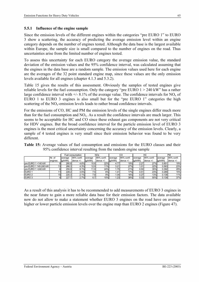
Emission Functions for Heavy Duty Vehicles 65
Federal Environment Agency – Austria BE-223 (2003)
5.5.1 Influence of the engine sample
Since the emission levels of the different engines within the categories “pre EURO 1” to EURO 3 show a scattering, the accuracy of predicting the average emission level within an engine category depends on the number of engines tested. Although the data base is the largest available within Europe, the sample size is small compared to the number of engines on the road. Thus uncertainties arise from the limited number of engines tested.
To assess this uncertainty for each EURO category the average emission value, the standard deviation of the emission values and the 95% confidence interval, was calculated assuming that the engines in the data base are a random sample. The emission values used here for each engine are the averages of the 32 point standard engine map, since these values are the only emission levels available for all engines (chapter 4.1.3 and 5.3.2).
Table 15 gives the results of this assessment. Obviously the samples of tested engines give reliable levels for the fuel consumption. Only the category “pre EURO 1 > 240 kW” has a rather large confidence interval with +/- 8.1% of the average value. The confidence intervals for NOx of EURO 1 to EURO 3 engines is also small but for the “pre EURO 1” categories the high scattering of the NOx-emission levels leads to rather broad confidence intervals.
For the emissions of CO, HC and PM the emission levels of the single engines differ much more than for the fuel consumption and NOx. As a result the confidence intervals are much larger. This seems to be acceptable for HC and CO since these exhaust gas components are not very critical for HDV engines. But the broad confidence interval for the particle emission level of EURO 3 engines is the most critical uncertainty concerning the accuracy of the emission levels. Clearly, a sample of 4 tested engines is very small since their emission behavior was found to be very different.
Table 15: Average values of fuel consumption and emissions for the EURO classes and their 95% confidence interval resulting from the random engine sample
Nr. of engines
average [g/kWh]
95% confi-dence +/-
average [g/kWh]
95% confi-dence +/-
average [g/kWh]
95% confi-dence +/-
average [g/kWh]
95% confi-dence +/-
average [g/kWh]
95% confi-dence +/-
pre EURO 1 <140 kW 8 280.8 4.6% 10.6 22% 4.77 19% 2.27 27% 0.851 19%pre EURO 1 140-240 kW 13 266.3 4.3% 12.9 11% 3.21 27% 1.01 22% 0.563 23%pre EURO 1 >240 kW 6 255.9 8.1% 11.9 24% 1.75 21% 0.50 35% 0.392 29%EURO 1 11 228.2 3.5% 7.5 6% 1.41 17% 0.51 23% 0.289 15%EURO 2 15 220.3 2.1% 7.8 9% 1.04 16% 0.27 13% 0.138 11%EURO 3 4 227.7 2.7% 6.7 10% 1.23 38% 0.33 50% 0.139 37%
PMFuel consumption NOx CO HC
As a result of this analysis it has to be recommended to add measurements of EURO 3 engines in the near future to gain a more reliable data base for their emission factors. The data available now do not allow to make a statement whether EURO 3 engines on the road have on average higher or lower particle emission levels over the engine map than EURO 2 engines (Figure 47).
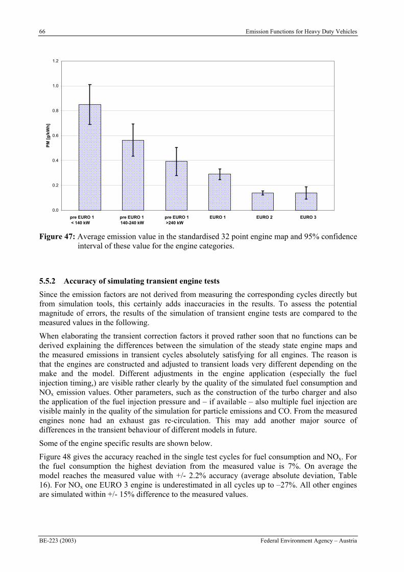
66 Emission Functions for Heavy Duty Vehicles
BE-223 (2003) Federal Environment Agency – Austria
0.0
0.2
0.4
0.6
0.8
1.0
1.2
1
PM
[g
/kW
h]
pre EURO 1 pre EURO 1 pre EURO 1 EURO 1 EURO 2 EURO 3 < 140 kW 140-240 kW >240 kW
Figure 47: Average emission value in the standardised 32 point engine map and 95% confidence interval of these value for the engine categories.
5.5.2 Accuracy of simulating transient engine tests
Since the emission factors are not derived from measuring the corresponding cycles directly but from simulation tools, this certainly adds inaccuracies in the results. To assess the potential magnitude of errors, the results of the simulation of transient engine tests are compared to the measured values in the following.
When elaborating the transient correction factors it proved rather soon that no functions can be derived explaining the differences between the simulation of the steady state engine maps and the measured emissions in transient cycles absolutely satisfying for all engines. The reason is that the engines are constructed and adjusted to transient loads very different depending on the make and the model. Different adjustments in the engine application (especially the fuel injection timing,) are visible rather clearly by the quality of the simulated fuel consumption and NOx emission values. Other parameters, such as the construction of the turbo charger and also the application of the fuel injection pressure and – if available – also multiple fuel injection are visible mainly in the quality of the simulation for particle emissions and CO. From the measured engines none had an exhaust gas re-circulation. This may add another major source of differences in the transient behaviour of different models in future.
Some of the engine specific results are shown below.
Figure 48 gives the accuracy reached in the single test cycles for fuel consumption and NOx. For the fuel consumption the highest deviation from the measured value is 7%. On average the model reaches the measured value with +/- 2.2% accuracy (average absolute deviation, Table 16). For NOx one EURO 3 engine is underestimated in all cycles up to –27%. All other engines are simulated within +/- 15% difference to the measured values.
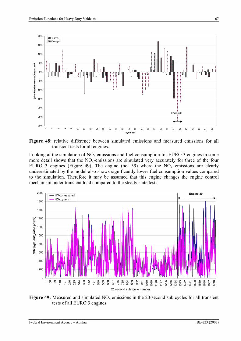
Emission Functions for Heavy Duty Vehicles 67
Federal Environment Agency – Austria BE-223 (2003)
-30%
-25%
-20%
-15%
-10%
-5%
0%
5%
10%
15%
20%
1 3 5 7 9 11 13 15 17 19 21 23 25 27 29 31 33 35 37 39 41 43 45 47 49 51 53
cycle Nr.
(sim
ula
ted
-mea
sure
d)/
mea
sure
d
FC-dyn.
NOx-dyn.
Engine 39
Figure 48: relative difference between simulated emissions and measured emissions for all transient tests for all engines.
Looking at the simulation of NOx emissions and fuel consumption for EURO 3 engines in some more detail shows that the NOx-emissions are simulated very accurately for three of the four EURO 3 engines (Figure 49). The engine (no. 39) where the NOx emissions are clearly underestimated by the model also shows significantly lower fuel consumption values compared to the simulation. Therefore it may be assumed that this engine changes the engine control mechanism under transient load compared to the steady state tests.
0
200
400
600
800
1000
1200
1400
1600
1800
2000
1 50 99
148
197
246
295
344
393
442
491
540
589
638
687
736
785
834
883
932
981
1030
1079
1128
1177
1226
1275
1324
1373
1422
1471
1520
1569
1618
1667
1716
20 second sub cycle number
NO
x [(
g/h
)/kW
_rat
ed p
ow
er]
NOx_measured
NOx_phem
Engine 39
Figure 49: Measured and simulated NOx emissions in the 20-second sub cycles for all transient tests of all EURO 3 engines.
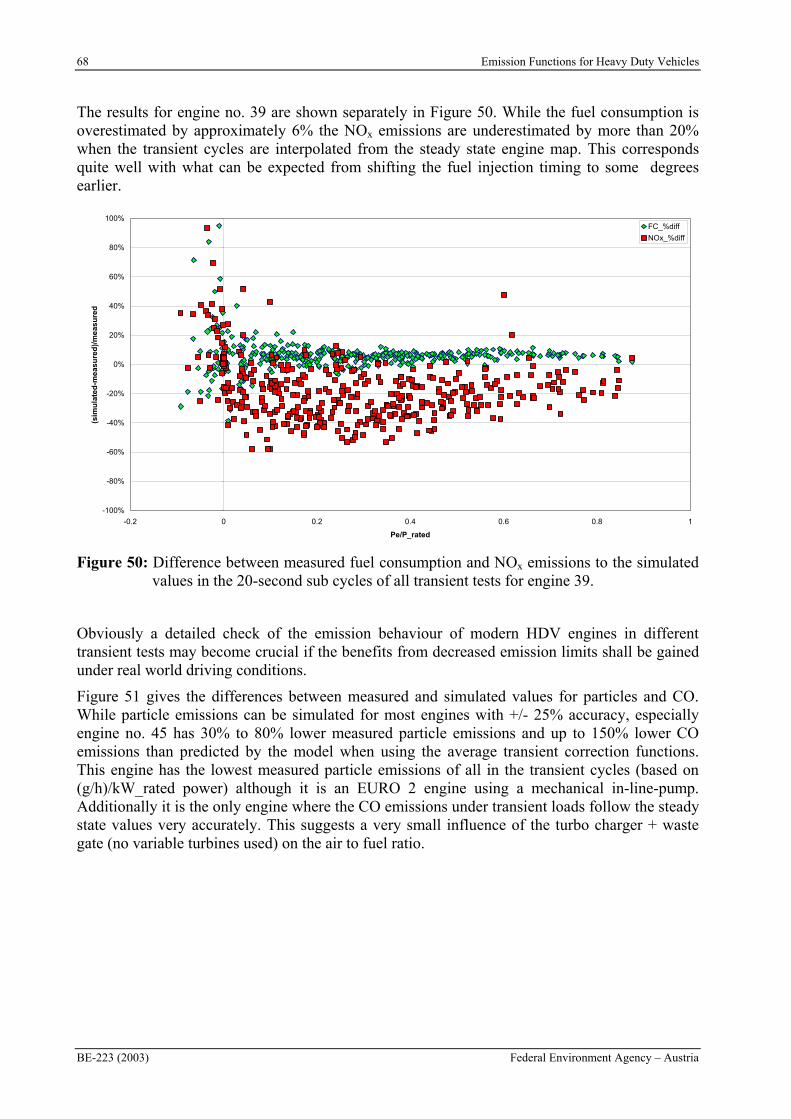
68 Emission Functions for Heavy Duty Vehicles
BE-223 (2003) Federal Environment Agency – Austria
The results for engine no. 39 are shown separately in Figure 50. While the fuel consumption is overestimated by approximately 6% the NOx emissions are underestimated by more than 20% when the transient cycles are interpolated from the steady state engine map. This corresponds quite well with what can be expected from shifting the fuel injection timing to some degrees earlier.
-100%
-80%
-60%
-40%
-20%
0%
20%
40%
60%
80%
100%
-0.2 0 0.2 0.4 0.6 0.8 1
Pe/P_rated
(sim
ula
ted
-mea
sure
d)/
mea
sure
d
FC_%diff
NOx_%diff
Figure 50: Difference between measured fuel consumption and NOx emissions to the simulated values in the 20-second sub cycles of all transient tests for engine 39.
Obviously a detailed check of the emission behaviour of modern HDV engines in different transient tests may become crucial if the benefits from decreased emission limits shall be gained under real world driving conditions.
Figure 51 gives the differences between measured and simulated values for particles and CO. While particle emissions can be simulated for most engines with +/- 25% accuracy, especially engine no. 45 has 30% to 80% lower measured particle emissions and up to 150% lower CO emissions than predicted by the model when using the average transient correction functions. This engine has the lowest measured particle emissions of all in the transient cycles (based on (g/h)/kW_rated power) although it is an EURO 2 engine using a mechanical in-line-pump. Additionally it is the only engine where the CO emissions under transient loads follow the steady state values very accurately. This suggests a very small influence of the turbo charger + waste gate (no variable turbines used) on the air to fuel ratio.
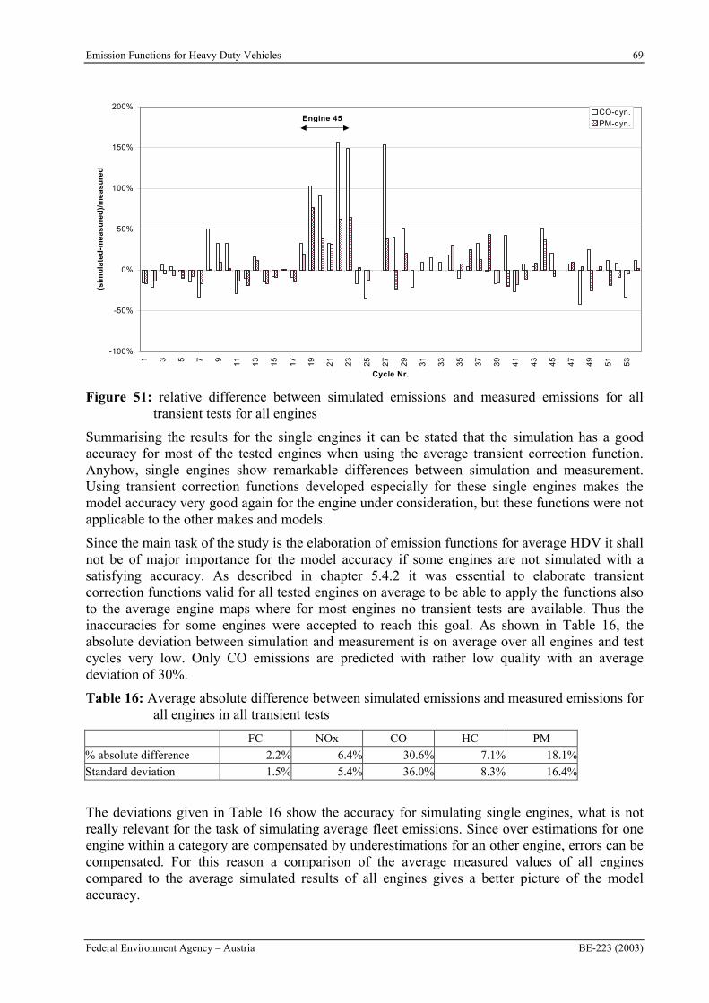
Emission Functions for Heavy Duty Vehicles 69
Federal Environment Agency – Austria BE-223 (2003)
-100%
-50%
0%
50%
100%
150%
200%
1 3 5 7 9
11
13
15
17
19
21
23
25
27
29
31
33
35
37
39
41
43
45
47
49
51
53
Cycle Nr.
(sim
ula
ted
-me
as
ure
d)/
me
as
ure
d
CO-dyn.
PM-dyn.Engine 45
Figure 51: relative difference between simulated emissions and measured emissions for all transient tests for all engines
Summarising the results for the single engines it can be stated that the simulation has a good accuracy for most of the tested engines when using the average transient correction function. Anyhow, single engines show remarkable differences between simulation and measurement. Using transient correction functions developed especially for these single engines makes the model accuracy very good again for the engine under consideration, but these functions were not applicable to the other makes and models.
Since the main task of the study is the elaboration of emission functions for average HDV it shall not be of major importance for the model accuracy if some engines are not simulated with a satisfying accuracy. As described in chapter 5.4.2 it was essential to elaborate transient correction functions valid for all tested engines on average to be able to apply the functions also to the average engine maps where for most engines no transient tests are available. Thus the inaccuracies for some engines were accepted to reach this goal. As shown in Table 16, the absolute deviation between simulation and measurement is on average over all engines and test cycles very low. Only CO emissions are predicted with rather low quality with an average deviation of 30%.
Table 16: Average absolute difference between simulated emissions and measured emissions for all engines in all transient tests
FC NOx CO HC PM
% absolute difference 2.2% 6.4% 30.6% 7.1% 18.1%
Standard deviation 1.5% 5.4% 36.0% 8.3% 16.4%
The deviations given in Table 16 show the accuracy for simulating single engines, what is not really relevant for the task of simulating average fleet emissions. Since over estimations for one engine within a category are compensated by underestimations for an other engine, errors can be compensated. For this reason a comparison of the average measured values of all engines compared to the average simulated results of all engines gives a better picture of the model accuracy.
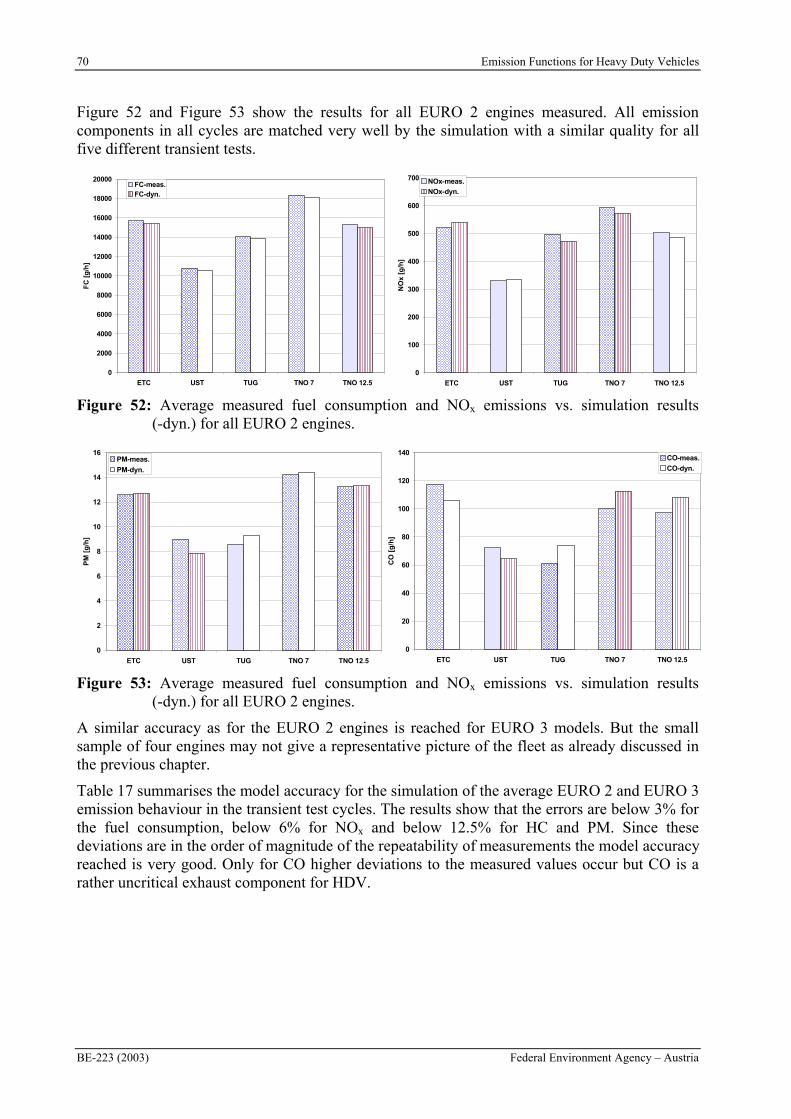
70 Emission Functions for Heavy Duty Vehicles
BE-223 (2003) Federal Environment Agency – Austria
Figure 52 and Figure 53 show the results for all EURO 2 engines measured. All emission components in all cycles are matched very well by the simulation with a similar quality for all five different transient tests.
0
2000
4000
6000
8000
10000
12000
14000
16000
18000
20000
ETC UST TUG TNO 7 TNO 12.5
FC
[g
/h]
FC-meas.FC-dyn.
0
100
200
300
400
500
600
700
ETC UST TUG TNO 7 TNO 12.5
NO
x [g
/h]
NOx-meas.
NOx-dyn.
Figure 52: Average measured fuel consumption and NOx emissions vs. simulation results (-dyn.) for all EURO 2 engines.
0
20
40
60
80
100
120
140
ETC UST TUG TNO 7 TNO 12.5
CO
[g
/h]
CO-meas.
CO-dyn.
0
2
4
6
8
10
12
14
16
ETC UST TUG TNO 7 TNO 12.5
PM
[g
/h]
PM-meas.
PM-dyn.
Figure 53: Average measured fuel consumption and NOx emissions vs. simulation results (-dyn.) for all EURO 2 engines.
A similar accuracy as for the EURO 2 engines is reached for EURO 3 models. But the small sample of four engines may not give a representative picture of the fleet as already discussed in the previous chapter.
Table 17 summarises the model accuracy for the simulation of the average EURO 2 and EURO 3 emission behaviour in the transient test cycles. The results show that the errors are below 3% for the fuel consumption, below 6% for NOx and below 12.5% for HC and PM. Since these deviations are in the order of magnitude of the repeatability of measurements the model accuracy reached is very good. Only for CO higher deviations to the measured values occur but CO is a rather uncritical exhaust component for HDV.
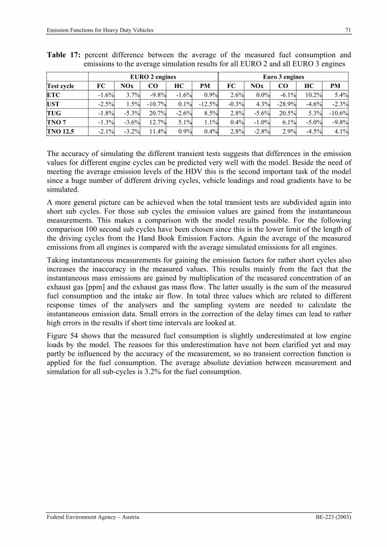
Emission Functions for Heavy Duty Vehicles 71
Federal Environment Agency – Austria BE-223 (2003)
Table 17: percent difference between the average of the measured fuel consumption and emissions to the average simulation results for all EURO 2 and all EURO 3 engines
EURO 2 engines Euro 3 engines
Test cycle FC NOx CO HC PM FC NOx CO HC PM
ETC -1.6% 3.7% -9.8% -1.6% 0.9% 2.6% 0.0% -6.1% 10.2% 5.4%
UST -2.5% 1.5% -10.7% 0.1% -12.5% -0.3% 4.3% -28.9% -4.6% -2.3%
TUG -1.8% -5.3% 20.7% -2.6% 8.5% 2.8% -5.6% 20.5% 5.3% -10.6%
TNO 7 -1.3% -3.6% 12.7% 5.1% 1.1% 0.4% -1.0% 6.1% -5.0% -9.8%
TNO 12.5 -2.1% -3.2% 11.4% 0.9% 0.4% 2.8% -2.8% 2.9% -4.5% 4.1%
The accuracy of simulating the different transient tests suggests that differences in the emission values for different engine cycles can be predicted very well with the model. Beside the need of meeting the average emission levels of the HDV this is the second important task of the model since a huge number of different driving cycles, vehicle loadings and road gradients have to be simulated.
A more general picture can be achieved when the total transient tests are subdivided again into short sub cycles. For those sub cycles the emission values are gained from the instantaneous measurements. This makes a comparison with the model results possible. For the following comparison 100 second sub cycles have been chosen since this is the lower limit of the length of the driving cycles from the Hand Book Emission Factors. Again the average of the measured emissions from all engines is compared with the average simulated emissions for all engines.
Taking instantaneous measurements for gaining the emission factors for rather short cycles also increases the inaccuracy in the measured values. This results mainly from the fact that the instantaneous mass emissions are gained by multiplication of the measured concentration of an exhaust gas [ppm] and the exhaust gas mass flow. The latter usually is the sum of the measured fuel consumption and the intake air flow. In total three values which are related to different response times of the analysers and the sampling system are needed to calculate the instantaneous emission data. Small errors in the correction of the delay times can lead to rather high errors in the results if short time intervals are looked at.
Figure 54 shows that the measured fuel consumption is slightly underestimated at low engine loads by the model. The reasons for this underestimation have not been clarified yet and may partly be influenced by the accuracy of the measurement, so no transient correction function is applied for the fuel consumption. The average absolute deviation between measurement and simulation for all sub-cycles is 3.2% for the fuel consumption.
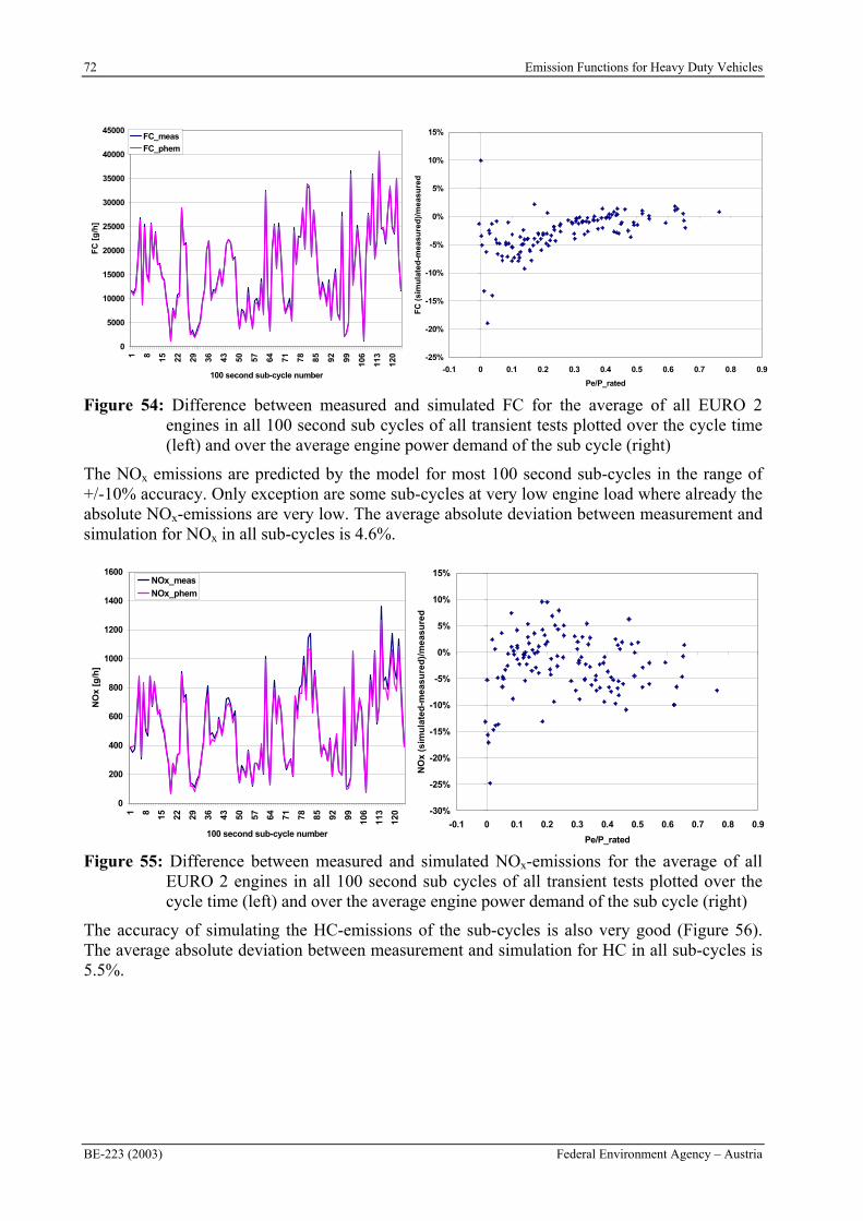
72 Emission Functions for Heavy Duty Vehicles
BE-223 (2003) Federal Environment Agency – Austria
0
5000
10000
15000
20000
25000
30000
35000
40000
450001 8 15 22 29 36 43 50 57 64 71 78 85 92 99
106
113
120
100 second sub-cycle number
FC
[g
/h]
FC_meas
FC_phem
-25%
-20%
-15%
-10%
-5%
0%
5%
10%
15%
-0.1 0 0.1 0.2 0.3 0.4 0.5 0.6 0.7 0.8 0.9
Pe/P_rated
FC
(si
mu
late
d-m
easu
red
)/m
easu
red
Figure 54: Difference between measured and simulated FC for the average of all EURO 2 engines in all 100 second sub cycles of all transient tests plotted over the cycle time (left) and over the average engine power demand of the sub cycle (right)
The NOx emissions are predicted by the model for most 100 second sub-cycles in the range of +/-10% accuracy. Only exception are some sub-cycles at very low engine load where already the absolute NOx-emissions are very low. The average absolute deviation between measurement and simulation for NOx in all sub-cycles is 4.6%.
0
200
400
600
800
1000
1200
1400
1600
1 8 15 22 29 36 43 50 57 64 71 78 85 92 99 106
113
120
100 second sub-cycle number
NO
x [g
/h]
NOx_meas
NOx_phem
-30%
-25%
-20%
-15%
-10%
-5%
0%
5%
10%
15%
-0.1 0 0.1 0.2 0.3 0.4 0.5 0.6 0.7 0.8 0.9
Pe/P_rated
NO
x (s
imu
late
d-m
easu
red
)/m
easu
red
Figure 55: Difference between measured and simulated NOx-emissions for the average of all EURO 2 engines in all 100 second sub cycles of all transient tests plotted over the cycle time (left) and over the average engine power demand of the sub cycle (right)
The accuracy of simulating the HC-emissions of the sub-cycles is also very good (Figure 56). The average absolute deviation between measurement and simulation for HC in all sub-cycles is 5.5%.
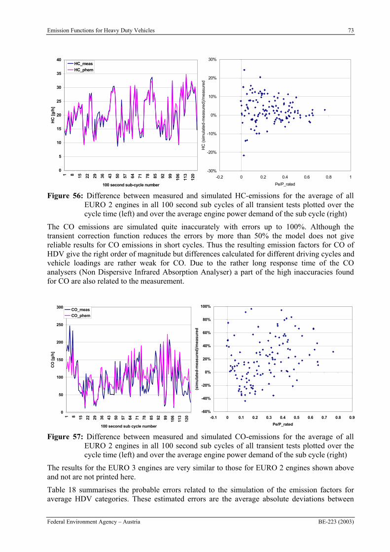
Emission Functions for Heavy Duty Vehicles 73
Federal Environment Agency – Austria BE-223 (2003)
0
5
10
15
20
25
30
35
401 8
15 22 29 36 43 50 57 64 71 78 85 92 99 106
113
120
100 second sub-cycle number
HC
[g
/h]
HC_meas
HC_phem
-30%
-20%
-10%
0%
10%
20%
30%
-0.2 0 0.2 0.4 0.6 0.8 1
Pe/P_rated
HC
(si
mu
late
d-m
ea
sure
d)/
me
asu
red
Figure 56: Difference between measured and simulated HC-emissions for the average of all EURO 2 engines in all 100 second sub cycles of all transient tests plotted over the cycle time (left) and over the average engine power demand of the sub cycle (right)
The CO emissions are simulated quite inaccurately with errors up to 100%. Although the transient correction function reduces the errors by more than 50% the model does not give reliable results for CO emissions in short cycles. Thus the resulting emission factors for CO of HDV give the right order of magnitude but differences calculated for different driving cycles and vehicle loadings are rather weak for CO. Due to the rather long response time of the CO analysers (Non Dispersive Infrared Absorption Analyser) a part of the high inaccuracies found for CO are also related to the measurement.
0
50
100
150
200
250
300
1 8 15 22 29 36 43 50 57 64 71 78 85 92 99
106
113
120
100 second sub cycle number
CO
[g
/h]
CO_meas
CO_phem
-60%
-40%
-20%
0%
20%
40%
60%
80%
100%
-0.1 0 0.1 0.2 0.3 0.4 0.5 0.6 0.7 0.8 0.9
Pe/P_rated
(sim
ula
ted
-mea
sure
d)/
mea
sure
d
Figure 57: Difference between measured and simulated CO-emissions for the average of all EURO 2 engines in all 100 second sub cycles of all transient tests plotted over the cycle time (left) and over the average engine power demand of the sub cycle (right)
The results for the EURO 3 engines are very similar to those for EURO 2 engines shown above and not are not printed here.
Table 18 summarises the probable errors related to the simulation of the emission factors for average HDV categories. These estimated errors are the average absolute deviations between
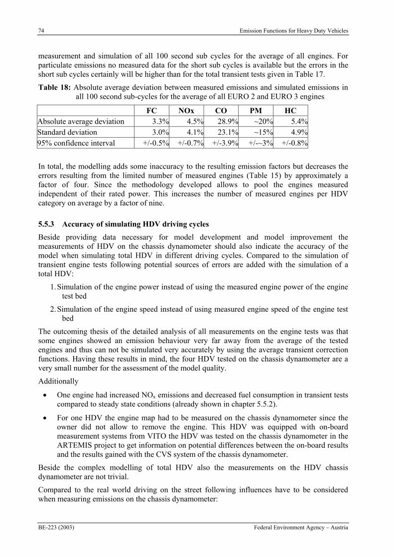
74 Emission Functions for Heavy Duty Vehicles
BE-223 (2003) Federal Environment Agency – Austria
measurement and simulation of all 100 second sub cycles for the average of all engines. For particulate emissions no measured data for the short sub cycles is available but the errors in the short sub cycles certainly will be higher than for the total transient tests given in Table 17.
Table 18: Absolute average deviation between measured emissions and simulated emissions in all 100 second sub-cycles for the average of all EURO 2 and EURO 3 engines
FC NOx CO PM HC Absolute average deviation 3.3% 4.5% 28.9% ~20% 5.4%Standard deviation 3.0% 4.1% 23.1% ~15% 4.9%95% confidence interval +/-0.5% +/-0.7% +/-3.9% +/-~3% +/-0.8%
In total, the modelling adds some inaccuracy to the resulting emission factors but decreases the errors resulting from the limited number of measured engines (Table 15) by approximately a factor of four. Since the methodology developed allows to pool the engines measured independent of their rated power. This increases the number of measured engines per HDV category on average by a factor of nine.
5.5.3 Accuracy of simulating HDV driving cycles
Beside providing data necessary for model development and model improvement the measurements of HDV on the chassis dynamometer should also indicate the accuracy of the model when simulating total HDV in different driving cycles. Compared to the simulation of transient engine tests following potential sources of errors are added with the simulation of a total HDV:
1. Simulation of the engine power instead of using the measured engine power of the engine test bed
2. Simulation of the engine speed instead of using measured engine speed of the engine test bed
The outcoming thesis of the detailed analysis of all measurements on the engine tests was that some engines showed an emission behaviour very far away from the average of the tested engines and thus can not be simulated very accurately by using the average transient correction functions. Having these results in mind, the four HDV tested on the chassis dynamometer are a very small number for the assessment of the model quality.
Additionally
One engine had increased NOx emissions and decreased fuel consumption in transient tests compared to steady state conditions (already shown in chapter 5.5.2).
For one HDV the engine map had to be measured on the chassis dynamometer since the owner did not allow to remove the engine. This HDV was equipped with on-board measurement systems from VITO the HDV was tested on the chassis dynamometer in the ARTEMIS project to get information on potential differences between the on-board results and the results gained with the CVS system of the chassis dynamometer.
Beside the complex modelling of total HDV also the measurements on the HDV chassis dynamometer are not trivial.
Compared to the real world driving on the street following influences have to be considered when measuring emissions on the chassis dynamometer:
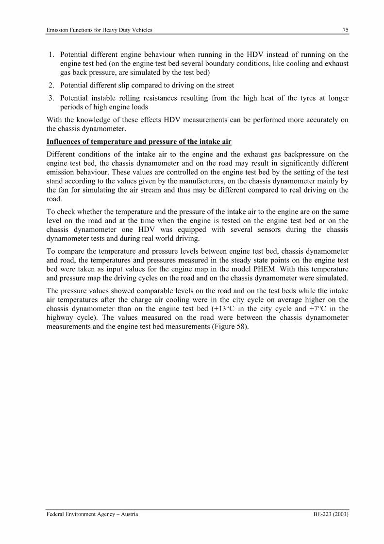
Emission Functions for Heavy Duty Vehicles 75
Federal Environment Agency – Austria BE-223 (2003)
1. Potential different engine behaviour when running in the HDV instead of running on the engine test bed (on the engine test bed several boundary conditions, like cooling and exhaust gas back pressure, are simulated by the test bed)
2. Potential different slip compared to driving on the street
3. Potential instable rolling resistances resulting from the high heat of the tyres at longer periods of high engine loads
With the knowledge of these effects HDV measurements can be performed more accurately on the chassis dynamometer.
Influences of temperature and pressure of the intake air
Different conditions of the intake air to the engine and the exhaust gas backpressure on the engine test bed, the chassis dynamometer and on the road may result in significantly different emission behaviour. These values are controlled on the engine test bed by the setting of the test stand according to the values given by the manufacturers, on the chassis dynamometer mainly by the fan for simulating the air stream and thus may be different compared to real driving on the road.
To check whether the temperature and the pressure of the intake air to the engine are on the same level on the road and at the time when the engine is tested on the engine test bed or on the chassis dynamometer one HDV was equipped with several sensors during the chassis dynamometer tests and during real world driving.
To compare the temperature and pressure levels between engine test bed, chassis dynamometer and road, the temperatures and pressures measured in the steady state points on the engine test bed were taken as input values for the engine map in the model PHEM. With this temperature and pressure map the driving cycles on the road and on the chassis dynamometer were simulated.
The pressure values showed comparable levels on the road and on the test beds while the intake air temperatures after the charge air cooling were in the city cycle on average higher on the chassis dynamometer than on the engine test bed (+13°C in the city cycle and +7°C in the highway cycle). The values measured on the road were between the chassis dynamometer measurements and the engine test bed measurements (Figure 58).
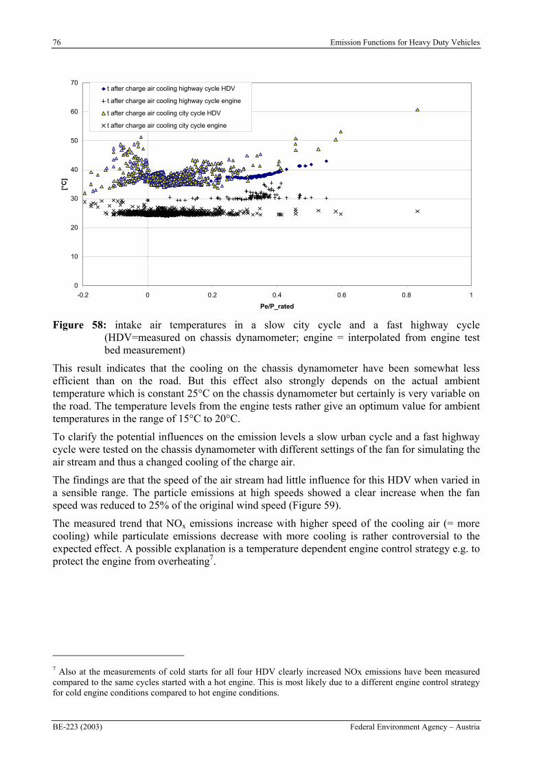
76 Emission Functions for Heavy Duty Vehicles
BE-223 (2003) Federal Environment Agency – Austria
0
10
20
30
40
50
60
70
-0.2 0 0.2 0.4 0.6 0.8 1
Pe/P_rated
[°C
]
t after charge air cooling highway cycle HDV
t after charge air cooling highway cycle engine
t after charge air cooling city cycle HDV
t after charge air cooling city cycle engine
Figure 58: intake air temperatures in a slow city cycle and a fast highway cycle (HDV=measured on chassis dynamometer; engine = interpolated from engine test bed measurement)
This result indicates that the cooling on the chassis dynamometer have been somewhat less efficient than on the road. But this effect also strongly depends on the actual ambient temperature which is constant 25°C on the chassis dynamometer but certainly is very variable on the road. The temperature levels from the engine tests rather give an optimum value for ambient temperatures in the range of 15°C to 20°C.
To clarify the potential influences on the emission levels a slow urban cycle and a fast highway cycle were tested on the chassis dynamometer with different settings of the fan for simulating the air stream and thus a changed cooling of the charge air.
The findings are that the speed of the air stream had little influence for this HDV when varied in a sensible range. The particle emissions at high speeds showed a clear increase when the fan speed was reduced to 25% of the original wind speed (Figure 59).
The measured trend that NOx emissions increase with higher speed of the cooling air (= more cooling) while particulate emissions decrease with more cooling is rather controversial to the expected effect. A possible explanation is a temperature dependent engine control strategy e.g. to protect the engine from overheating7.
7 Also at the measurements of cold starts for all four HDV clearly increased NOx emissions have been measured compared to the same cycles started with a hot engine. This is most likely due to a different engine control strategy for cold engine conditions compared to hot engine conditions.
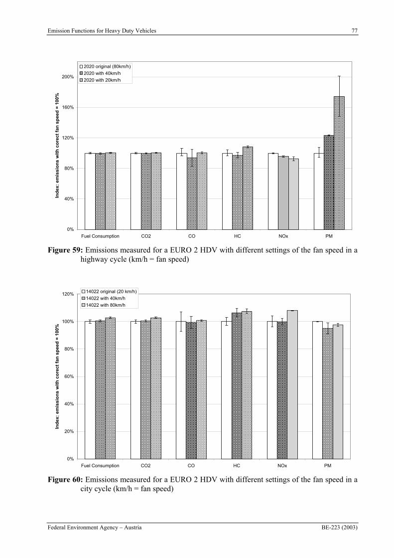
Emission Functions for Heavy Duty Vehicles 77
Federal Environment Agency – Austria BE-223 (2003)
0%
40%
80%
120%
160%
200%
Fuel Consumption CO2 CO HC NOx PM
Ind
ex:
emis
sio
ns
wit
h c
ore
ct f
an s
pee
d =
100
%
2020 original (80km/h)
2020 with 40km/h
2020 with 20km/h
Figure 59: Emissions measured for a EURO 2 HDV with different settings of the fan speed in a highway cycle (km/h = fan speed)
0%
20%
40%
60%
80%
100%
120%
Fuel Consumption CO2 CO HC NOx PM
Ind
ex:
emis
sio
ns
wit
h c
ore
ct f
an s
pee
d =
100
%
14022 original (20 km/h)
14022 with 40km/h
14022 with 80km/h
Figure 60: Emissions measured for a EURO 2 HDV with different settings of the fan speed in a city cycle (km/h = fan speed)
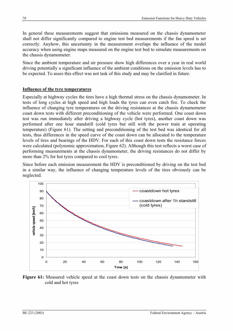
78 Emission Functions for Heavy Duty Vehicles
BE-223 (2003) Federal Environment Agency – Austria
In general these measurements suggest that emissions measured on the chassis dynamometer shall not differ significantly compared to engine test bed measurements if the fan speed is set correctly. Anyhow, this uncertainty in the measurement overlaps the influence of the model accuracy when using engine maps measured on the engine test bed to simulate measurements on the chassis dynamometer.
Since the ambient temperature and air pressure show high differences over a year in real world driving potentially a significant influence of the ambient conditions on the emission levels has to be expected. To asses this effect was not task of this study and may be clarified in future.
Influence of the tyre temperatures
Especially at highway cycles the tires have a high thermal stress on the chassis dynamometer. In tests of long cycles at high speed and high loads the tyres can even catch fire. To check the influence of changing tyre temperatures on the driving resistances at the chassis dynamometer coast down tests with different preconditioning of the vehicle were performed. One coast down test was run immediately after driving a highway cycle (hot tyres), another coast down was performed after one hour standstill (cold tyres but still with the power train at operating temperature) (Figure 61). The setting and preconditioning of the test bed was identical for all tests, thus differences in the speed curve of the coast down can be allocated to the temperature levels of tires and bearings of the HDV. For each of this coast down tests the resistance forces were calculated (polynomic approximation, Figure 62). Although this test reflects a worst case of performing measurements at the chassis dynamometer, the driving resistances do not differ by more than 2% for hot tyres compared to cool tyres.
Since before each emission measurement the HDV is preconditioned by driving on the test bed in a similar way, the influence of changing temperature levels of the tires obviously can be neglected.
0
10
20
30
40
50
60
70
80
90
100
0 20 40 60 80 100 120 140 160
Time [s]
vehi
cle
spee
d [k
m/h
]
coastdown hot tyres
coastdown after 1h standstill(cold tyres)
Figure 61: Measured vehicle speed at the coast down tests on the chassis dynamometer with cold and hot tyres
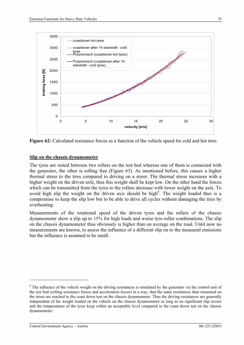
Emission Functions for Heavy Duty Vehicles 79
Federal Environment Agency – Austria BE-223 (2003)
0
500
1000
1500
2000
2500
3000
3500
0 5 10 15 20 25 30
velocity [m/s]
bra
kin
g fo
rce
[N]
coastdown hot tyres
coastdown after 1h standstill - coldtyresPolynomisch (coastdown hot tyres)
Polynomisch (coastdown after 1hstandstill - cold tyres)
Figure 62: Calculated resistance forces as a function of the vehicle speed for cold and hot tires
Slip on the chassis dynamometer
The tyres are rested between two rollers on the test bed whereas one of them is connected with the generator, the other is rolling free (Figure 63). As mentioned before, this causes a higher thermal stress to the tires compared to driving on a street. The thermal stress increases with a higher weight on the driven axle, thus this weight shall be kept low. On the other hand the forces which can be transmitted from the tyres to the rollers decrease with lower weight on the axle. To avoid high slip the weight on the driven axis should be high8. The weight loaded thus is a compromise to keep the slip low but to be able to drive all cycles without damaging the tires by overheating.
Measurements of the rotational speed of the driven tyres and the rollers of the chassis dynamometer show a slip up to 15% for high loads and worse tyre-roller combinations. The slip on the chassis dynamometer thus obviously is higher than on average on the road. Until now no measurements are known, to assess the influence of a different slip on to the measured emissions but the influence is assumed to be small.
8 The influence of the vehicle weight on the driving resistances is simulated by the generator via the control unit of the test bed (rolling resistance forces and acceleration forces) in a way, that the same resistances than measured on the street are reached in the coast down test on the chassis dynamometer. Thus the driving resistances are generally independent of the weight loaded on the vehicle on the chassis dynamometer as long as no significant slip occurs and the temperatures of the tyres keep within an acceptable level compared to the coast down test on the chassis dynamometer.
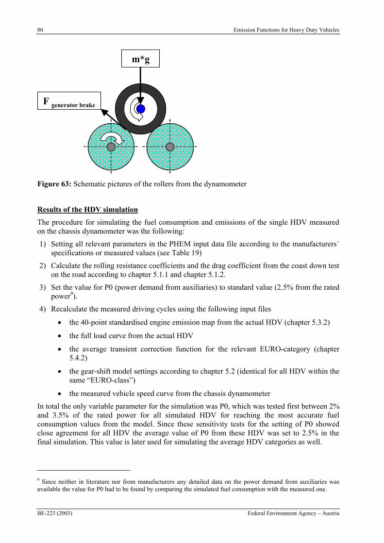
80 Emission Functions for Heavy Duty Vehicles
BE-223 (2003) Federal Environment Agency – Austria
m*g
F generator brake
Figure 63: Schematic pictures of the rollers from the dynamometer
Results of the HDV simulation
The procedure for simulating the fuel consumption and emissions of the single HDV measured on the chassis dynamometer was the following:
1) Setting all relevant parameters in the PHEM input data file according to the manufacturers´ specifications or measured values (see Table 19)
2) Calculate the rolling resistance coefficients and the drag coefficient from the coast down test on the road according to chapter 5.1.1 and chapter 5.1.2.
3) Set the value for P0 (power demand from auxiliaries) to standard value (2.5% from the rated power9).
4) Recalculate the measured driving cycles using the following input files
the 40-point standardised engine emission map from the actual HDV (chapter 5.3.2)
the full load curve from the actual HDV
the average transient correction function for the relevant EURO-category (chapter 5.4.2)
the gear-shift model settings according to chapter 5.2 (identical for all HDV within the same “EURO-class”)
the measured vehicle speed curve from the chassis dynamometer
In total the only variable parameter for the simulation was P0, which was tested first between 2% and 3.5% of the rated power for all simulated HDV for reaching the most accurate fuel consumption values from the model. Since these sensitivity tests for the setting of P0 showed close agreement for all HDV the average value of P0 from these HDV was set to 2.5% in the final simulation. This value is later used for simulating the average HDV categories as well.
9 Since neither in literature nor from manufacturers any detailed data on the power demand from auxiliaries was available the value for P0 had to be found by comparing the simulated fuel consumption with the measured one.
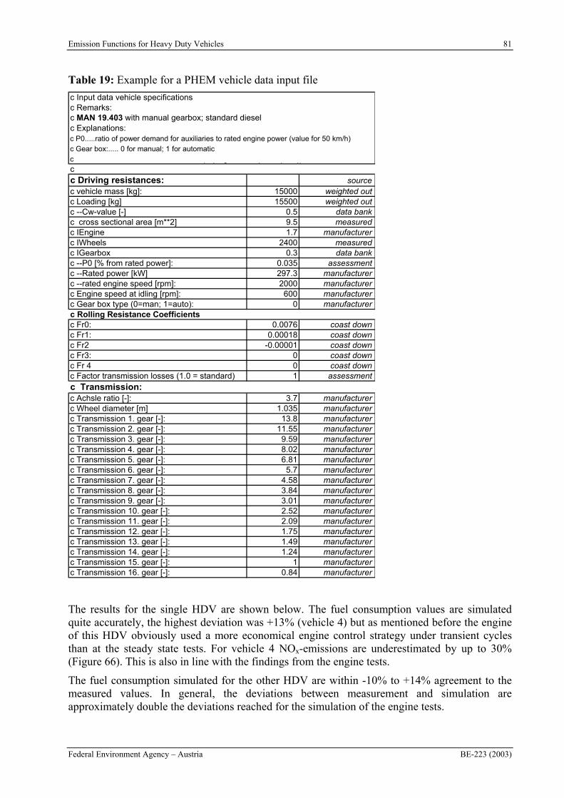
Emission Functions for Heavy Duty Vehicles 81
Federal Environment Agency – Austria BE-223 (2003)
Table 19: Example for a PHEM vehicle data input file
c Input data vehicle specificationsc Remarks:c MAN 19.403 with manual gearbox; standard dieselc Explanations:c P0.....ratio of power demand for auxiliaries to rated engine power (value for 50 km/h)c Gear box:..... 0 for manual; 1 for automaticc Delta.......Drehmassefaktor for 50km/h (in programme F(veh. Speed))cc Driving resistances: sourcec vehicle mass [kg]: 15000 weighted outc Loading [kg] 15500 weighted outc --Cw-value [-] 0.5 data bankc cross sectional area [m**2] 9.5 measuredc IEngine 1.7 manufacturerc IWheels 2400 measuredc IGearbox 0.3 data bankc --P0 [% from rated power]: 0.035 assessmentc --Rated power [kW] 297.3 manufacturerc --rated engine speed [rpm]: 2000 manufacturerc Engine speed at idling [rpm]: 600 manufacturerc Gear box type (0=man; 1=auto): 0 manufacturerc Rolling Resistance Coefficientsc Fr0: 0.0076 coast downc Fr1: 0.00018 coast downc Fr2 -0.00001 coast downc Fr3: 0 coast downc Fr 4 0 coast downc Factor transmission losses (1.0 = standard) 1 assessmentc Transmission:c Achsle ratio [-]: 3.7 manufacturerc Wheel diameter [m] 1.035 manufacturerc Transmission 1. gear [-]: 13.8 manufacturerc Transmission 2. gear [-]: 11.55 manufacturerc Transmission 3. gear [-]: 9.59 manufacturerc Transmission 4. gear [-]: 8.02 manufacturerc Transmission 5. gear [-]: 6.81 manufacturerc Transmission 6. gear [-]: 5.7 manufacturerc Transmission 7. gear [-]: 4.58 manufacturerc Transmission 8. gear [-]: 3.84 manufacturerc Transmission 9. gear [-]: 3.01 manufacturerc Transmission 10. gear [-]: 2.52 manufacturerc Transmission 11. gear [-]: 2.09 manufacturerc Transmission 12. gear [-]: 1.75 manufacturerc Transmission 13. gear [-]: 1.49 manufacturerc Transmission 14. gear [-]: 1.24 manufacturerc Transmission 15. gear [-]: 1 manufacturerc Transmission 16. gear [-]: 0.84 manufacturer
The results for the single HDV are shown below. The fuel consumption values are simulated quite accurately, the highest deviation was +13% (vehicle 4) but as mentioned before the engine of this HDV obviously used a more economical engine control strategy under transient cycles than at the steady state tests. For vehicle 4 NOx-emissions are underestimated by up to 30% (Figure 66). This is also in line with the findings from the engine tests.
The fuel consumption simulated for the other HDV are within -10% to +14% agreement to the measured values. In general, the deviations between measurement and simulation are approximately double the deviations reached for the simulation of the engine tests.
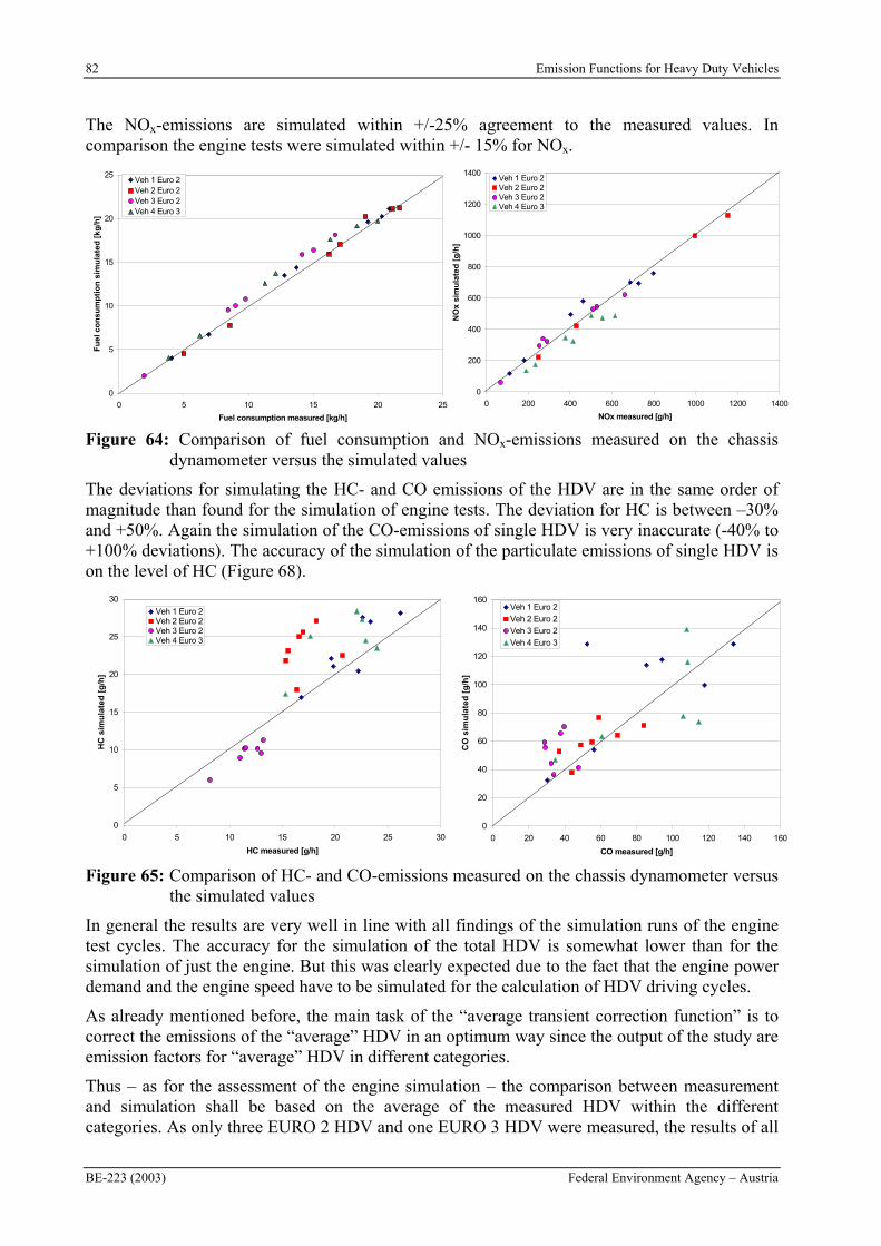
82 Emission Functions for Heavy Duty Vehicles
BE-223 (2003) Federal Environment Agency – Austria
The NOx-emissions are simulated within +/-25% agreement to the measured values. In comparison the engine tests were simulated within +/- 15% for NOx.
0
5
10
15
20
25
0 5 10 15 20 25
Fuel consumption measured [kg/h]
Fu
el c
on
sum
pti
on
sim
ula
ted
[kg
/h]
Veh 1 Euro 2Veh 2 Euro 2Veh 3 Euro 2Veh 4 Euro 3
0
200
400
600
800
1000
1200
1400
0 200 400 600 800 1000 1200 1400
NOx measured [g/h]
NO
x si
mu
late
d [
g/h
]
Veh 1 Euro 2Veh 2 Euro 2Veh 3 Euro 2Veh 4 Euro 3
Figure 64: Comparison of fuel consumption and NOx-emissions measured on the chassis dynamometer versus the simulated values
The deviations for simulating the HC- and CO emissions of the HDV are in the same order of magnitude than found for the simulation of engine tests. The deviation for HC is between –30% and +50%. Again the simulation of the CO-emissions of single HDV is very inaccurate (-40% to +100% deviations). The accuracy of the simulation of the particulate emissions of single HDV is on the level of HC (Figure 68).
0
5
10
15
20
25
30
0 5 10 15 20 25 30
HC measured [g/h]
HC
sim
ula
ted
[g
/h]
Veh 1 Euro 2Veh 2 Euro 2Veh 3 Euro 2Veh 4 Euro 3
0
20
40
60
80
100
120
140
160
0 20 40 60 80 100 120 140 160
CO measured [g/h]
CO
sim
ula
ted
[g
/h]
Veh 1 Euro 2
Veh 2 Euro 2
Veh 3 Euro 2
Veh 4 Euro 3
Figure 65: Comparison of HC- and CO-emissions measured on the chassis dynamometer versus the simulated values
In general the results are very well in line with all findings of the simulation runs of the engine test cycles. The accuracy for the simulation of the total HDV is somewhat lower than for the simulation of just the engine. But this was clearly expected due to the fact that the engine power demand and the engine speed have to be simulated for the calculation of HDV driving cycles.
As already mentioned before, the main task of the “average transient correction function” is to correct the emissions of the “average” HDV in an optimum way since the output of the study are emission factors for “average” HDV in different categories.
Thus – as for the assessment of the engine simulation – the comparison between measurement and simulation shall be based on the average of the measured HDV within the different categories. As only three EURO 2 HDV and one EURO 3 HDV were measured, the results of all
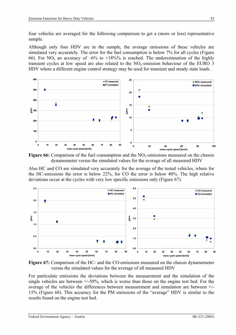
Emission Functions for Heavy Duty Vehicles 83
Federal Environment Agency – Austria BE-223 (2003)
four vehicles are averaged for the following comparison to get a (more or less) representative sample.
Although only four HDV are in the sample, the average emissions of these vehicles are simulated very accurately. The error for the fuel consumption is below 7% for all cycles (Figure 66). For NOx an accuracy of –6% to +18%% is reached. The underestimation of the highly transient cycles at low speed are also related to the NOx-emission behaviour of the EURO 3 HDV where a different engine control strategy may be used for transient and steady state loads.
0
100
200
300
400
500
600
0 10 20 30 40 50 60 70 80 90
mean cycle speed [km/h]
g/k
m
FC measured
FC simulated
0
5
10
15
20
25
0 20 40 60 80 100mean cycle speed [km/h]
g/k
m
NOx measured
NOx simulated
Figure 66: Comparison of the fuel consumption and the NOx-emissions measured on the chassis dynamometer versus the simulated values for the average of all measured HDV
Also HC and CO are simulated very accurately for the average of the tested vehicles, where for the HC-emissions the error is below 22%, for CO the error is below 40%. The high relative deviations occur at the cycles with very low specific emissions only (Figure 67).
0.0
0.5
1.0
1.5
2.0
2.5
0 10 20 30 40 50 60 70 80 90
mean cycle speed [km/h]
g/k
m
HC measured
HC simulated
0.0
1.0
2.0
3.0
4.0
5.0
6.0
0 10 20 30 40 50 60 70 80 90
mean cycle speed [km/h]
g/k
m
CO measured
CO simulated
Figure 67: Comparison of the HC- and the CO-emissions measured on the chassis dynamometer versus the simulated values for the average of all measured HDV
For particulate emissions the deviations between the measurement and the simulation of the single vehicles are between +/-50%, which is worse than those on the engine test bed. For the average of the vehicles the differences between measurement and simulation are between +/-15% (Figure 68). This accuracy for the PM emissions of the “average” HDV is similar to the results found on the engine test bed.
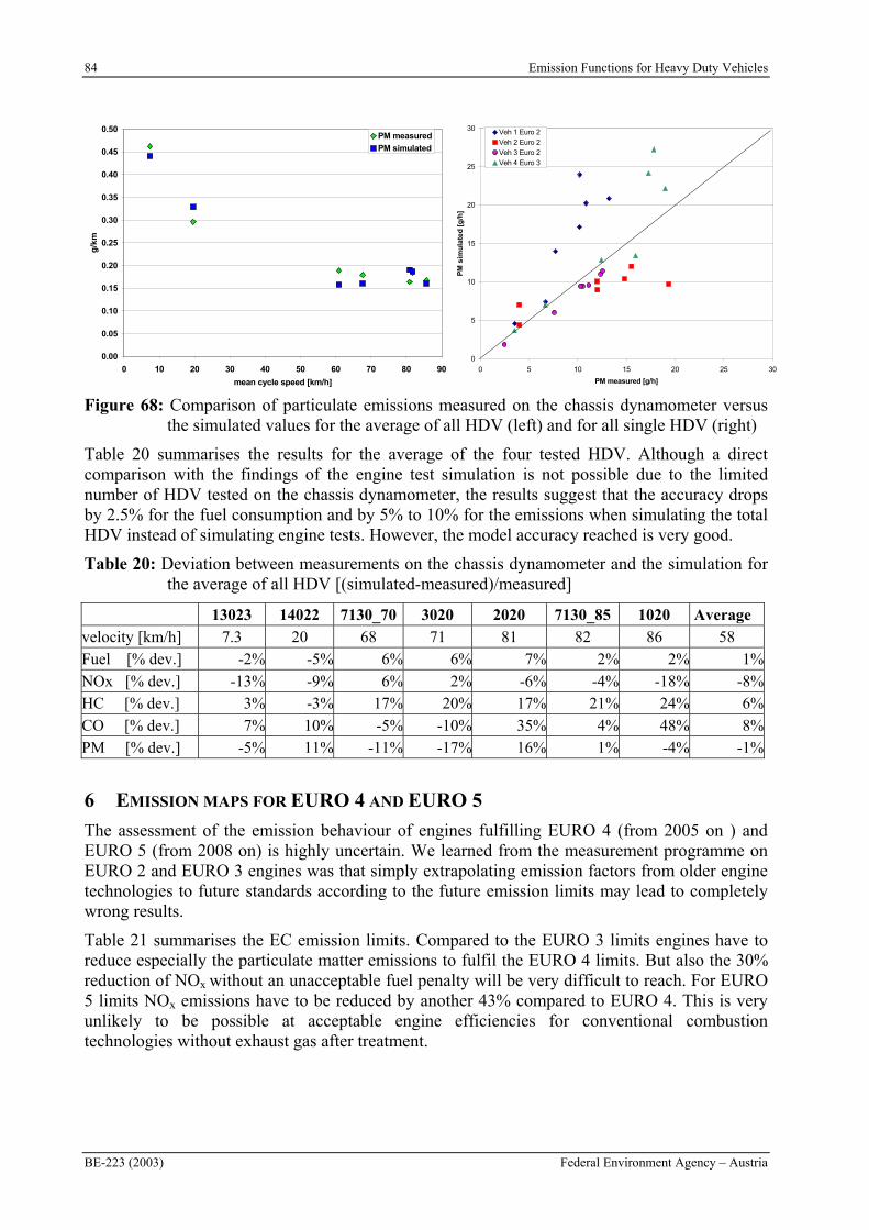
84 Emission Functions for Heavy Duty Vehicles
BE-223 (2003) Federal Environment Agency – Austria
0
5
10
15
20
25
30
0 5 10 15 20 25 30
PM measured [g/h]
PM
sim
ula
ted
[g
/h]
Veh 1 Euro 2
Veh 2 Euro 2Veh 3 Euro 2
Veh 4 Euro 3
0.00
0.05
0.10
0.15
0.20
0.25
0.30
0.35
0.40
0.45
0.50
0 10 20 30 40 50 60 70 80 90
mean cycle speed [km/h]
g/k
m
PM measured
PM simulated
Figure 68: Comparison of particulate emissions measured on the chassis dynamometer versus the simulated values for the average of all HDV (left) and for all single HDV (right)
Table 20 summarises the results for the average of the four tested HDV. Although a direct comparison with the findings of the engine test simulation is not possible due to the limited number of HDV tested on the chassis dynamometer, the results suggest that the accuracy drops by 2.5% for the fuel consumption and by 5% to 10% for the emissions when simulating the total HDV instead of simulating engine tests. However, the model accuracy reached is very good.
Table 20: Deviation between measurements on the chassis dynamometer and the simulation for the average of all HDV [(simulated-measured)/measured]
13023 14022 7130_70 3020 2020 7130_85 1020 Average velocity [km/h] 7.3 20 68 71 81 82 86 58 Fuel [% dev.] -2% -5% 6% 6% 7% 2% 2% 1%NOx [% dev.] -13% -9% 6% 2% -6% -4% -18% -8%HC [% dev.] 3% -3% 17% 20% 17% 21% 24% 6%CO [% dev.] 7% 10% -5% -10% 35% 4% 48% 8%PM [% dev.] -5% 11% -11% -17% 16% 1% -4% -1%
6 EMISSION MAPS FOR EURO 4 AND EURO 5
The assessment of the emission behaviour of engines fulfilling EURO 4 (from 2005 on ) and EURO 5 (from 2008 on) is highly uncertain. We learned from the measurement programme on EURO 2 and EURO 3 engines was that simply extrapolating emission factors from older engine technologies to future standards according to the future emission limits may lead to completely wrong results.
Table 21 summarises the EC emission limits. Compared to the EURO 3 limits engines have to reduce especially the particulate matter emissions to fulfil the EURO 4 limits. But also the 30% reduction of NOx without an unacceptable fuel penalty will be very difficult to reach. For EURO 5 limits NOx emissions have to be reduced by another 43% compared to EURO 4. This is very unlikely to be possible at acceptable engine efficiencies for conventional combustion technologies without exhaust gas after treatment.
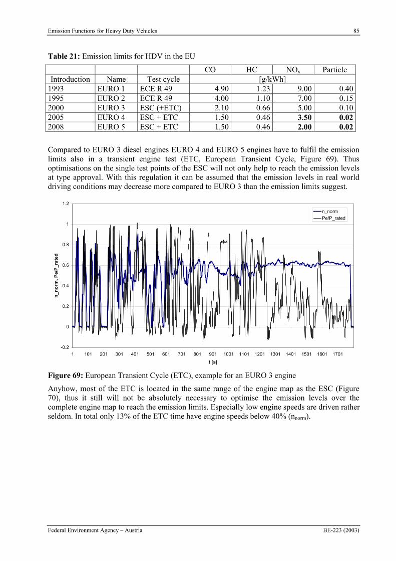
Emission Functions for Heavy Duty Vehicles 85
Federal Environment Agency – Austria BE-223 (2003)
Table 21: Emission limits for HDV in the EU
CO HC NOx Particle Introduction Name Test cycle [g/kWh]
1993 EURO 1 ECE R 49 4.90 1.23 9.00 0.401995 EURO 2 ECE R 49 4.00 1.10 7.00 0.152000 EURO 3 ESC (+ETC) 2.10 0.66 5.00 0.102005 EURO 4 ESC + ETC 1.50 0.46 3.50 0.022008 EURO 5 ESC + ETC 1.50 0.46 2.00 0.02
Compared to EURO 3 diesel engines EURO 4 and EURO 5 engines have to fulfil the emission limits also in a transient engine test (ETC, European Transient Cycle, Figure 69). Thus optimisations on the single test points of the ESC will not only help to reach the emission levels at type approval. With this regulation it can be assumed that the emission levels in real world driving conditions may decrease more compared to EURO 3 than the emission limits suggest.
-0.2
0
0.2
0.4
0.6
0.8
1
1.2
1 101 201 301 401 501 601 701 801 901 1001 1101 1201 1301 1401 1501 1601 1701
t [s]
n_n
orm
, P
e/P
_rat
ed
n_norm
Pe/P_rated
Figure 69: European Transient Cycle (ETC), example for an EURO 3 engine
Anyhow, most of the ETC is located in the same range of the engine map as the ESC (Figure 70), thus it still will not be absolutely necessary to optimise the emission levels over the complete engine map to reach the emission limits. Especially low engine speeds are driven rather seldom. In total only 13% of the ETC time have engine speeds below 40% (nnorm).
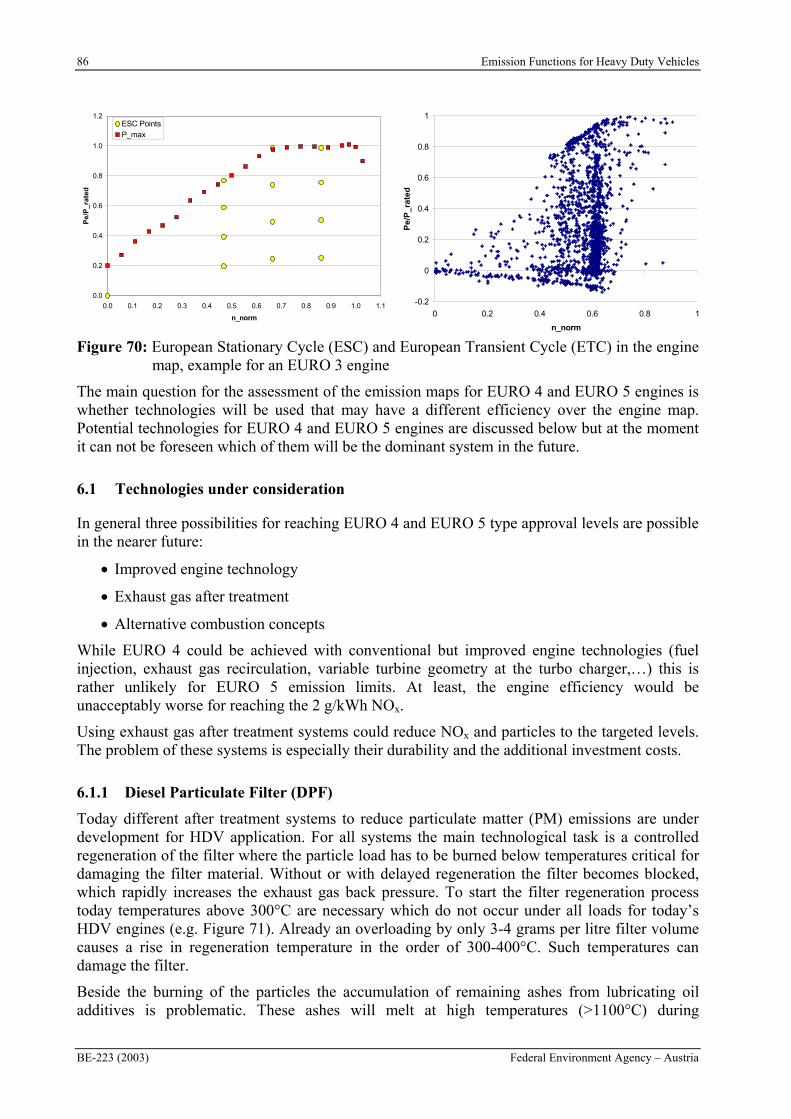
86 Emission Functions for Heavy Duty Vehicles
BE-223 (2003) Federal Environment Agency – Austria
0.0
0.2
0.4
0.6
0.8
1.0
1.2
0.0 0.1 0.2 0.3 0.4 0.5 0.6 0.7 0.8 0.9 1.0 1.1
n_norm
Pe
/P_
rate
d
ESC PointsP_max
-0.2
0
0.2
0.4
0.6
0.8
1
0 0.2 0.4 0.6 0.8 1
n_norm
Pe/
P_r
ated
Figure 70: European Stationary Cycle (ESC) and European Transient Cycle (ETC) in the engine map, example for an EURO 3 engine
The main question for the assessment of the emission maps for EURO 4 and EURO 5 engines is whether technologies will be used that may have a different efficiency over the engine map. Potential technologies for EURO 4 and EURO 5 engines are discussed below but at the moment it can not be foreseen which of them will be the dominant system in the future.
6.1 Technologies under consideration
In general three possibilities for reaching EURO 4 and EURO 5 type approval levels are possible in the nearer future:
Improved engine technology
Exhaust gas after treatment
Alternative combustion concepts
While EURO 4 could be achieved with conventional but improved engine technologies (fuel injection, exhaust gas recirculation, variable turbine geometry at the turbo charger,…) this is rather unlikely for EURO 5 emission limits. At least, the engine efficiency would be unacceptably worse for reaching the 2 g/kWh NOx.
Using exhaust gas after treatment systems could reduce NOx and particles to the targeted levels. The problem of these systems is especially their durability and the additional investment costs.
6.1.1 Diesel Particulate Filter (DPF)
Today different after treatment systems to reduce particulate matter (PM) emissions are under development for HDV application. For all systems the main technological task is a controlled regeneration of the filter where the particle load has to be burned below temperatures critical for damaging the filter material. Without or with delayed regeneration the filter becomes blocked, which rapidly increases the exhaust gas back pressure. To start the filter regeneration process today temperatures above 300°C are necessary which do not occur under all loads for today’s HDV engines (e.g. Figure 71). Already an overloading by only 3-4 grams per litre filter volume causes a rise in regeneration temperature in the order of 300-400°C. Such temperatures can damage the filter.
Beside the burning of the particles the accumulation of remaining ashes from lubricating oil additives is problematic. These ashes will melt at high temperatures (>1100°C) during
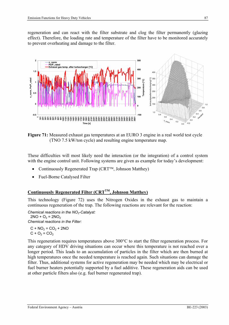
Emission Functions for Heavy Duty Vehicles 87
Federal Environment Agency – Austria BE-223 (2003)
regeneration and can react with the filter substrate and clog the filter permanently (glazing effect). Therefore, the loading rate and temperature of the filter have to be monitored accurately to prevent overheating and damage to the filter.
-0.2
0.0
0.2
0.4
0.6
0.8
1.0
Pe/ra
ted
0.00.2
0.40.6
0.81.0
n_norm
150
200
250
300
350
400
texh
au
stg
asa
fte
rtu
rbo
cha
rgin
g[°
C]
-0.5
0
0.5
1
1.5
2
110
120
130
140
150
160
170
180
190
110
0111
0112
0113
0114
0115
0116
0117
0118
0119
0120
0121
0122
0123
0124
0125
0126
0127
0128
0129
0130
0131
0132
0133
0134
0135
0136
0137
0138
01
Time [s]
n_n
orm
, P
e/P
_rat
ed
-100
0
100
200
300
400
500
Tem
per
atu
re [
°C]
n_normPe/P_ratedExhaust gas temp. after turbocharger [°C]
Figure 71: Measured exhaust gas temperatures at an EURO 3 engine in a real world test cycle (TNO 7.5 kW/ton cycle) and resulting engine temperature map.
These difficulties will most likely need the interaction (or the integration) of a control system with the engine control unit. Following systems are given as example for today’s development:
Continuously Regenerated Trap (CRT , Johnson Matthey)
Fuel-Borne Catalysed Filter
Continuously Regenerated Filter (CRTTM, Johnson Matthey)
This technology (Figure 72) uses the Nitrogen Oxides in the exhaust gas to maintain a continuous regeneration of the trap. The following reactions are relevant for the reaction:
Chemical reactions in the NO2-Catalyst: 2NO + O2 = 2NO2
Chemical reactions in the Filter:
C + NO2 = CO2 + 2NO C + O2 = CO2
This regeneration requires temperatures above 300°C to start the filter regeneration process. For any category of HDV driving situations can occur where this temperature is not reached over a longer period. This leads to an accumulation of particles in the filter which are then burned at high temperatures once the needed temperature is reached again. Such situations can damage the filter. Thus, additional systems for active regeneration may be needed which may be electrical or fuel burner heaters potentially supported by a fuel additive. These regeneration aids can be used at other particle filters also (e.g. fuel burner regenerated trap).
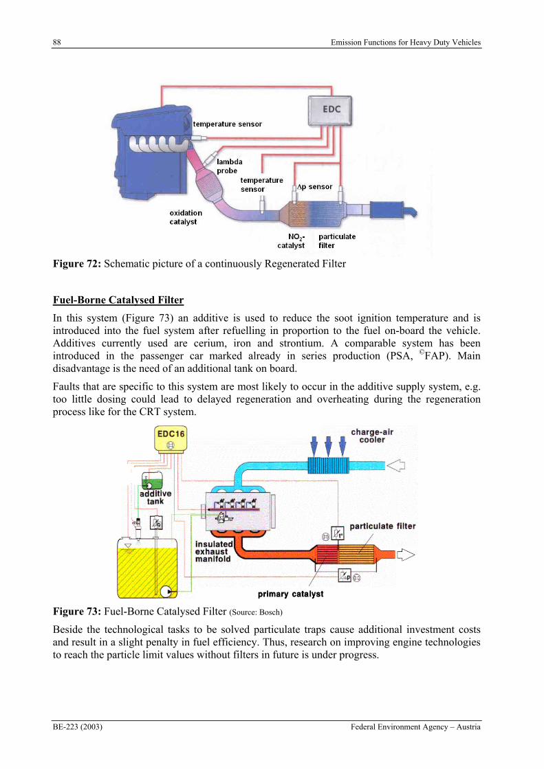
88 Emission Functions for Heavy Duty Vehicles
BE-223 (2003) Federal Environment Agency – Austria
Figure 72: Schematic picture of a continuously Regenerated Filter
Fuel-Borne Catalysed Filter
In this system (Figure 73) an additive is used to reduce the soot ignition temperature and is introduced into the fuel system after refuelling in proportion to the fuel on-board the vehicle. Additives currently used are cerium, iron and strontium. A comparable system has been introduced in the passenger car marked already in series production (PSA, ©FAP). Main disadvantage is the need of an additional tank on board.
Faults that are specific to this system are most likely to occur in the additive supply system, e.g. too little dosing could lead to delayed regeneration and overheating during the regeneration process like for the CRT system.
Figure 73: Fuel-Borne Catalysed Filter (Source: Bosch)
Beside the technological tasks to be solved particulate traps cause additional investment costs and result in a slight penalty in fuel efficiency. Thus, research on improving engine technologies to reach the particle limit values without filters in future is under progress.
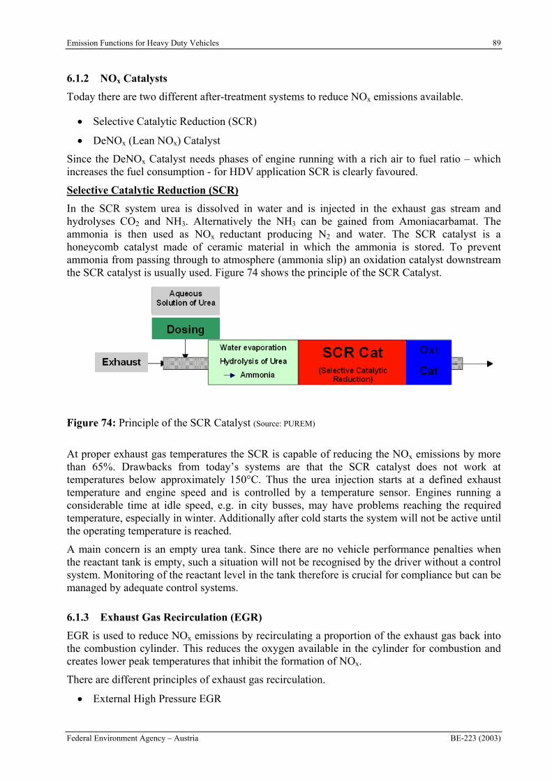
Emission Functions for Heavy Duty Vehicles 89
Federal Environment Agency – Austria BE-223 (2003)
6.1.2 NOx Catalysts
Today there are two different after-treatment systems to reduce NOx emissions available.
Selective Catalytic Reduction (SCR)
DeNOx (Lean NOx) Catalyst
Since the DeNOx Catalyst needs phases of engine running with a rich air to fuel ratio – which increases the fuel consumption - for HDV application SCR is clearly favoured.
Selective Catalytic Reduction (SCR)
In the SCR system urea is dissolved in water and is injected in the exhaust gas stream and hydrolyses CO2 and NH3. Alternatively the NH3 can be gained from Amoniacarbamat. The ammonia is then used as NOx reductant producing N2 and water. The SCR catalyst is a honeycomb catalyst made of ceramic material in which the ammonia is stored. To prevent ammonia from passing through to atmosphere (ammonia slip) an oxidation catalyst downstream the SCR catalyst is usually used. Figure 74 shows the principle of the SCR Catalyst.
Figure 74: Principle of the SCR Catalyst (Source: PUREM)
At proper exhaust gas temperatures the SCR is capable of reducing the NOx emissions by more than 65%. Drawbacks from today’s systems are that the SCR catalyst does not work at temperatures below approximately 150°C. Thus the urea injection starts at a defined exhaust temperature and engine speed and is controlled by a temperature sensor. Engines running a considerable time at idle speed, e.g. in city busses, may have problems reaching the required temperature, especially in winter. Additionally after cold starts the system will not be active until the operating temperature is reached.
A main concern is an empty urea tank. Since there are no vehicle performance penalties when the reactant tank is empty, such a situation will not be recognised by the driver without a control system. Monitoring of the reactant level in the tank therefore is crucial for compliance but can be managed by adequate control systems.
6.1.3 Exhaust Gas Recirculation (EGR)
EGR is used to reduce NOx emissions by recirculating a proportion of the exhaust gas back into the combustion cylinder. This reduces the oxygen available in the cylinder for combustion and creates lower peak temperatures that inhibit the formation of NOx.
There are different principles of exhaust gas recirculation.
External High Pressure EGR
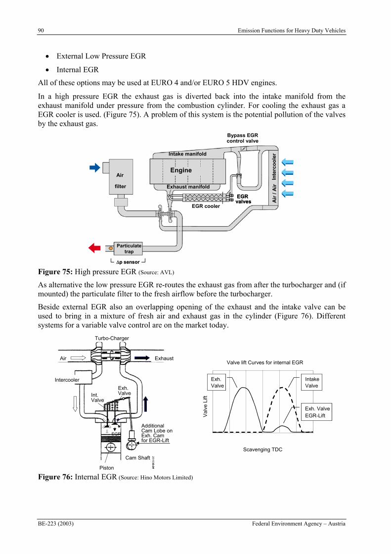
90 Emission Functions for Heavy Duty Vehicles
BE-223 (2003) Federal Environment Agency – Austria
External Low Pressure EGR
Internal EGR
All of these options may be used at EURO 4 and/or EURO 5 HDV engines.
In a high pressure EGR the exhaust gas is diverted back into the intake manifold from the exhaust manifold under pressure from the combustion cylinder. For cooling the exhaust gas a EGR cooler is used. (Figure 75). A problem of this system is the potential pollution of the valves by the exhaust gas.
EGR coolers
Bypass EGRcontrol valve
Intake manifold
Exhaust manifold
Engine
EGR on/offvalves
CRTTM
Airfilter
Air flowmeter
Air
/ A
ir I
nte
rco
ole
r
Ven
turi
pp sensor sensor pp sensor sensor
EGR cooler
EGRvalvesEGRvalves
Air
filter
Intake manifold
Air
/ A
irIn
terc
oo
ler
Engine
Exhaust manifold
Particulatetrap
Figure 75: High pressure EGR (Source: AVL)
As alternative the low pressure EGR re-routes the exhaust gas from after the turbocharger and (if mounted) the particulate filter to the fresh airflow before the turbocharger.
Beside external EGR also an overlapping opening of the exhaust and the intake valve can be used to bring in a mixture of fresh air and exhaust gas in the cylinder (Figure 76). Different systems for a variable valve control are on the market today.
Turbo-Charger
ExhaustAir
Intercooler
Cam Shaft
AdditionalCam Lobe on Exh. Camfor EGR-Lift
Exh.ValveInt.
Valve
Piston
EGR
201030-04
Turbo-Charger
ExhaustAir
Intercooler
Cam Shaft
AdditionalCam Lobe on Exh. Camfor EGR-Lift
Exh.ValveInt.
Valve
Piston
EGR
201030-04
90 180 270 360 450 540 630
Val
veLi
ft
Scavenging TDC
Valve lift Curves for internal EGR
IntakeValve
Exh.Valve
Exh. ValveEGR-Lift
Figure 76: Internal EGR (Source: Hino Motors Limited)
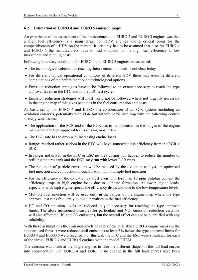
Emission Functions for Heavy Duty Vehicles 91
Federal Environment Agency – Austria BE-223 (2003)
6.2 Estimation of EURO 4 and EURO 5 emission maps
An experience of the assessment of the measurements on EURO 2 and EURO 3 engines was that a high fuel efficiency is a main target for HDV engines and a crucial point for the competitiveness of a HDV on the market. It certainly has to be assumed that also for EURO 4 and EURO 5 the manufacturers have to find solutions with a high fuel efficiency at low investment and running costs.
Following boundary conditions for EURO 4 and EURO 5 engines are assumed:
The technological solution for reaching future emission limits is not clear today
For different typical operational conditions of different HDV there may even be different combinations of the before mentioned technological options
Emission reduction strategies have to be followed to an extent necessary to reach the type approval levels in the ETC and in the ESC test cycles
Emission reduction strategies will most likely not be followed where not urgently necessary in the engine map if this gives penalties in the fuel consumption and costs
As basic set up for EURO 4 and EURO 5 a combination of an SCR system (including an oxidation catalyst), potentially with EGR but without particulate trap with the following control strategy was assumed:
The application of the SCR and of the EGR has to be optimised in the ranges of the engine map where the type approval test is driving most often
The EGR rate has to drop with increasing engine loads
Ranges reached rather seldom in the ETC will have somewhat less efficiency from the EGR + SCR
In ranges not driven in the ETC or ESC no urea dosing will happen to reduce the number of refilling the urea tank and the EGR may run with lower EGR rates
The reduction of particle emissions will be realised by the oxidation catalyst, an optimised fuel injection and combustion in combination with multiple fuel injection
For the efficiency of the oxidation catalyst even with less than 10 ppm Sulphur content the efficiency drops at high engine loads due to sulphate formation. At lower engine loads, especially with high engine speeds the efficiency drops also due to the low temperature levels.
Multiple fuel injection will be used only in the ranges of the engine map where the type approval test runs frequently to avoid penalties in the fuel efficiency
HC and CO emission levels are reduced only if necessary for reaching the type approval limits. The afore mentioned measures for particulate and NOx emission reduction certainly will also affect the HC and CO emissions, but the overall effect can not be quantified with any reliability.
With these assumptions the emission levels of each of the available EURO 3 engine maps (in the standardised format) were reduced until emissions at least 5% below the type approval limits for EURO 4 and EURO 5 were reached. For this task the ETC and the ESC were simulated for each of the virtual EURO 4 and EURO 5 engines with the model PHEM.
The exercise was made at the single engines to take the different shapes of the full load curves into consideration. For EURO 4 and EURO 5 no change in the full load curves have been
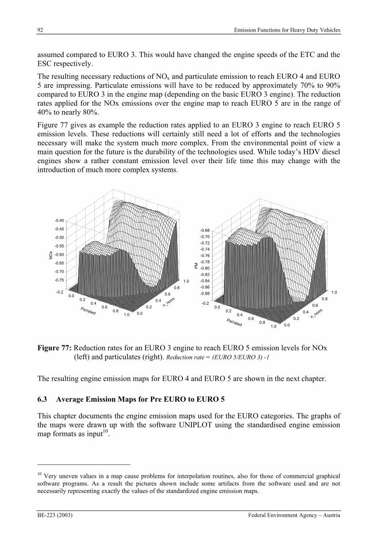
92 Emission Functions for Heavy Duty Vehicles
BE-223 (2003) Federal Environment Agency – Austria
assumed compared to EURO 3. This would have changed the engine speeds of the ETC and the ESC respectively.
The resulting necessary reductions of NOx and particulate emission to reach EURO 4 and EURO 5 are impressing. Particulate emissions will have to be reduced by approximately 70% to 90% compared to EURO 3 in the engine map (depending on the basic EURO 3 engine). The reduction rates applied for the NOx emissions over the engine map to reach EURO 5 are in the range of 40% to nearly 80%.
Figure 77 gives as example the reduction rates applied to an EURO 3 engine to reach EURO 5 emission levels. These reductions will certainly still need a lot of efforts and the technologies necessary will make the system much more complex. From the environmental point of view a main question for the future is the durability of the technologies used. While today’s HDV diesel engines show a rather constant emission level over their life time this may change with the introduction of much more complex systems.
-0.20.0
0.20.4
0.60.8
1.0
Pe/rated 0.0
0.2
0.4
0.6
0.8
1.0
n_norm
-0.75
-0.70
-0.65
-0.60
-0.55
-0.50
-0.45
-0.40
NO
x
-0.20.0
0.20.4
0.60.8
1.0
Pe/rated 0.0
0.2
0.4
0.6
0.8
1.0
n_norm
-0.88
-0.86
-0.84
-0.82
-0.80
-0.78
-0.76
-0.74
-0.72
-0.70
-0.68
PM
Figure 77: Reduction rates for an EURO 3 engine to reach EURO 5 emission levels for NOx (left) and particulates (right). Reduction rate = (EURO 5/EURO 3) -1
The resulting engine emission maps for EURO 4 and EURO 5 are shown in the next chapter.
6.3 Average Emission Maps for Pre EURO to EURO 5
This chapter documents the engine emission maps used for the EURO categories. The graphs of the maps were drawn up with the software UNIPLOT using the standardised engine emission map formats as input10.
10 Very uneven values in a map cause problems for interpolation routines, also for those of commercial graphical software programs. As a result the pictures shown include some artifacts from the software used and are not necessarily representing exactly the values of the standardized engine emission maps.
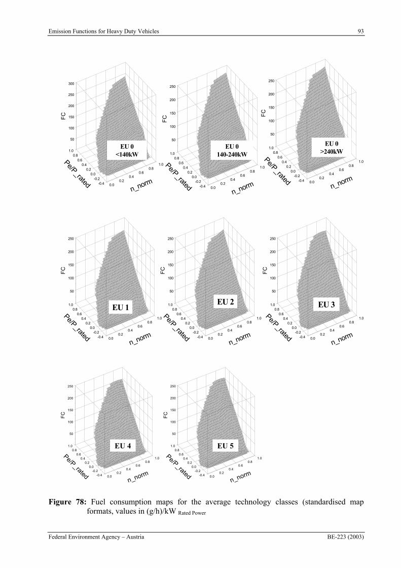
Emission Functions for Heavy Duty Vehicles 93
Federal Environment Agency – Austria BE-223 (2003)
-0.4-0.2
0.00.2
0.40.6
0.81.0
Pe/P_rated 0.00.2
0.40.6
0.81.0
n_norm
50
100
150
200
250
FC
-0.4-0.2
0.00.2
0.40.6
0.81.0
Pe/P_rated 0.00.2
0.40.6
0.81.0
n_norm
50
100
150
200
250
300
FC
-0.4-0.2
0.00.2
0.40.6
0.81.0
Pe/P_rated 0.00.2
0.40.6
0.81.0
n_norm
50
100
150
200
250
FC
EU 0140-240kW
EU 0<140kW
EU 0>240kW
-0.4-0.2
0.00.2
0.40.6
0.81.0
Pe/P_rated 0.00.2
0.40.6
0.81.0
n_norm
50
100
150
200
250
FC
EU 3
-0.4-0.2
0.00.2
0.40.6
0.81.0
Pe/P_rated 0.00.2
0.40.6
0.81.0
n_norm
50
100
150
200
250
FC
EU 2
-0.4-0.2
0.00.2
0.40.6
0.81.0
Pe/P_rated 0.00.2
0.40.6
0.81.0
n_norm
50
100
150
200
250
FC
EU 1
-0.4-0.2
0.00.2
0.40.6
0.81.0
Pe/P_rated 0.00.2
0.40.6
0.81.0
n_norm
50
100
150
200
250
FC
-0.4-0.2
0.00.2
0.40.6
0.81.0
Pe/P_rated 0.00.2
0.40.6
0.81.0
n_norm
50
100
150
200
250
FC
EU 5EU 4
Figure 78: Fuel consumption maps for the average technology classes (standardised map formats, values in (g/h)/kW Rated Power
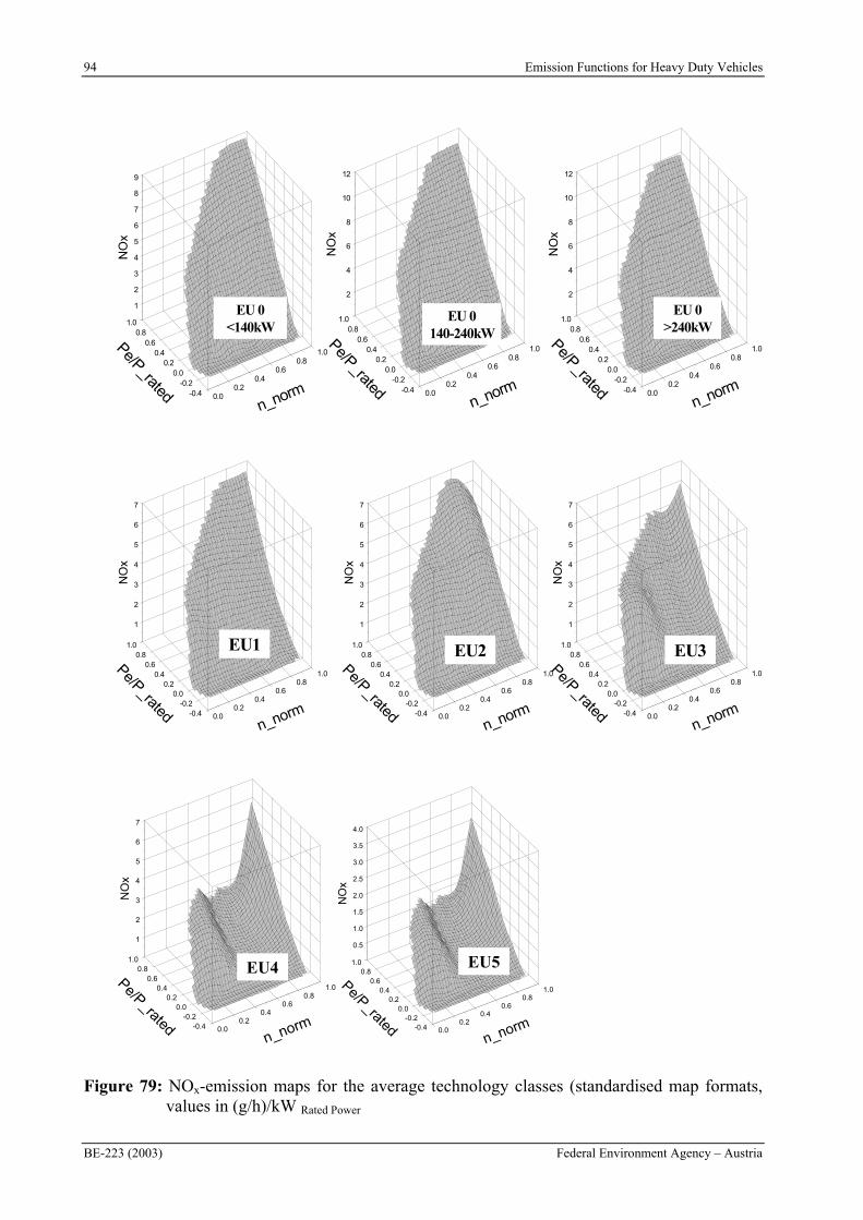
94 Emission Functions for Heavy Duty Vehicles
BE-223 (2003) Federal Environment Agency – Austria
-0.4-0.2
0.00.2
0.40.6
0.81.0
Pe/P_rated 0.00.2
0.40.6
0.81.0
n_norm
2
4
6
8
10
12
NO
x
-0.4-0.2
0.00.2
0.40.6
0.81.0
Pe/P_rated 0.00.2
0.40.6
0.81.0
n_norm
1
2
3
4
5
6
7
8
9
NO
x
-0.4-0.2
0.00.2
0.40.6
0.81.0
Pe/P_rated 0.00.2
0.40.6
0.81.0
n_norm
2
4
6
8
10
12
NO
x
EU 0140-240kW
EU 0<140kW
EU 0>240kW
-0.4-0.2
0.00.2
0.40.6
0.81.0
Pe/P_rated 0.00.2
0.40.6
0.81.0
n_norm
1
2
3
4
5
6
7
NO
x
EU3
-0.4-0.2
0.00.2
0.40.6
0.81.0
Pe/P_rated 0.00.2
0.40.6
0.81.0
n_norm
1
2
3
4
5
6
7
NO
x
EU2
-0.4-0.2
0.00.2
0.40.6
0.81.0
Pe/P_rated 0.00.2
0.40.6
0.81.0
n_norm
1
2
3
4
5
6
7
NO
x
EU1
-0.4-0.2
0.00.2
0.40.6
0.81.0
Pe/P_rated 0.00.2
0.40.6
0.81.0
n_norm
1
2
3
4
5
6
7
NO
x
-0.4-0.2
0.00.2
0.40.6
0.81.0
Pe/P_rated 0.00.2
0.40.6
0.81.0
n_norm
0.5
1.0
1.5
2.0
2.5
3.0
3.5
4.0
NO
x
EU4 EU5
Figure 79: NOx-emission maps for the average technology classes (standardised map formats, values in (g/h)/kW Rated Power
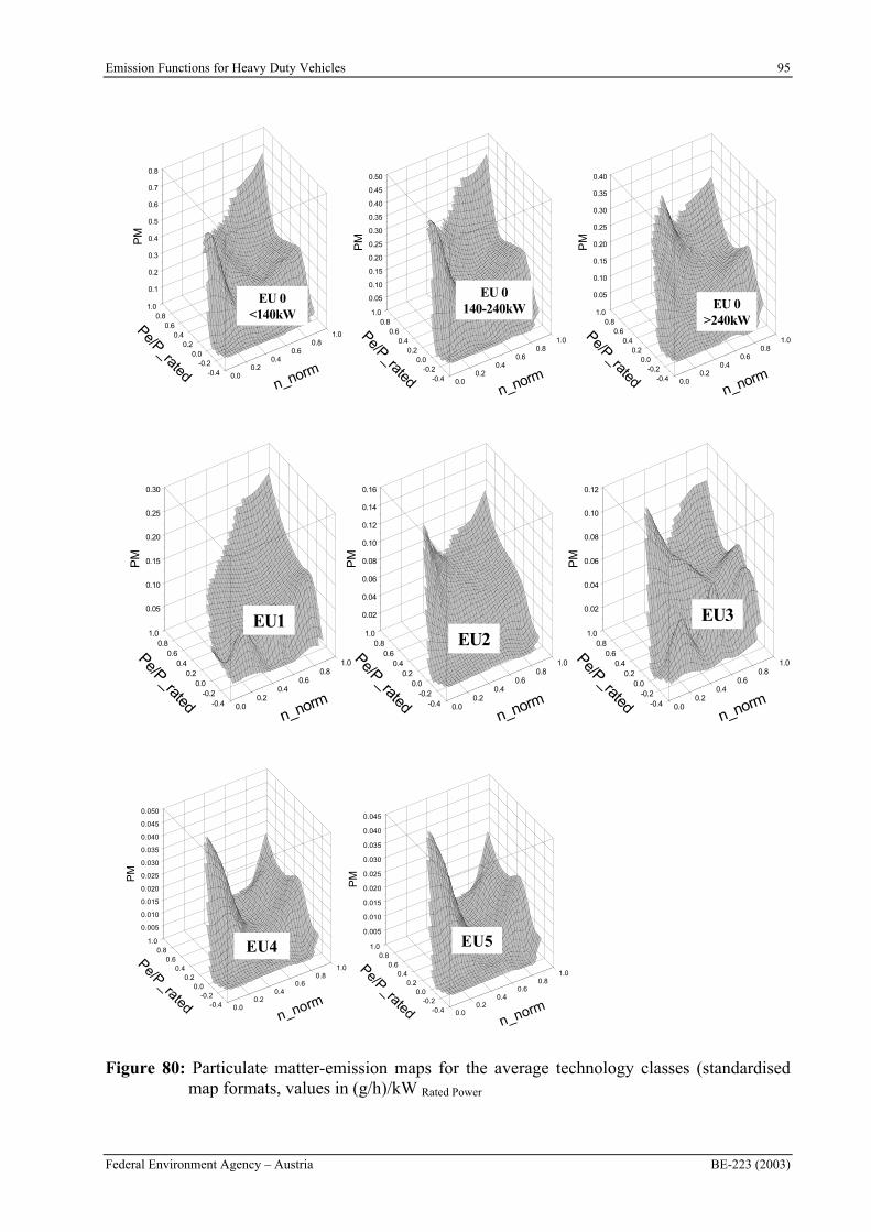
Emission Functions for Heavy Duty Vehicles 95
Federal Environment Agency – Austria BE-223 (2003)
-0.4-0.2
0.00.2
0.40.6
0.81.0
Pe/P_rated 0.00.2
0.40.6
0.81.0
n_norm
0.05
0.10
0.15
0.20
0.25
0.30
0.35
0.40
0.45
0.50
PM
-0.4-0.2
0.00.2
0.40.6
0.81.0
Pe/P_rated 0.00.2
0.40.6
0.81.0
n_norm
0.1
0.2
0.3
0.4
0.5
0.6
0.7
0.8
PM
-0.4-0.2
0.00.2
0.40.6
0.81.0
Pe/P_rated 0.00.2
0.40.6
0.81.0
n_norm
0.05
0.10
0.15
0.20
0.25
0.30
0.35
0.40
PM
EU 0140-240kW
EU 0<140kW
EU 0>240kW
-0.4-0.2
0.00.2
0.40.6
0.81.0
Pe/P_rated 0.00.2
0.40.6
0.81.0
n_norm
0.02
0.04
0.06
0.08
0.10
0.12
PM
EU3
-0.4-0.2
0.00.2
0.40.6
0.81.0
Pe/P_rated 0.00.2
0.40.6
0.81.0
n_norm
0.02
0.04
0.06
0.08
0.10
0.12
0.14
0.16
PM
EU2
-0.4-0.2
0.00.2
0.40.6
0.81.0
Pe/P_rated 0.00.2
0.40.6
0.81.0
n_norm
0.05
0.10
0.15
0.20
0.25
0.30
PM
EU1
-0.4-0.2
0.00.2
0.40.6
0.81.0
Pe/P_rated 0.00.2
0.40.6
0.81.0
n_norm
0.005
0.010
0.015
0.020
0.025
0.030
0.035
0.040
0.045
0.050
PM
-0.4-0.2
0.00.2
0.40.6
0.81.0
Pe/P_rated 0.00.2
0.40.6
0.81.0
n_norm
0.005
0.010
0.015
0.020
0.025
0.030
0.035
0.040
0.045
PM
EU4 EU5
Figure 80: Particulate matter-emission maps for the average technology classes (standardised map formats, values in (g/h)/kW Rated Power
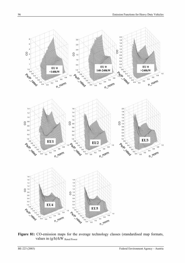
96 Emission Functions for Heavy Duty Vehicles
BE-223 (2003) Federal Environment Agency – Austria
-0.4-0.2
0.00.2
0.40.6
0.81.0
Pe/P_rated 0.00.2
0.40.6
0.81.0
n_norm
0.5
1.0
1.5
2.0
2.5
3.0
CO
-0.4-0.2
0.00.2
0.40.6
0.81.0
Pe/P_rated 0.00.2
0.40.6
0.81.0
n_norm
1
2
3
4
5
6
CO
-0.4-0.2
0.00.2
0.40.6
0.81.0
Pe/P_rated 0.00.2
0.40.6
0.81.0
n_norm
0.2
0.4
0.6
0.8
1.0
1.2
1.4
1.6
1.8
2.0
CO
EU 0140-240kW
EU 0<140kW
EU 0>240kW
-0.4-0.2
0.00.2
0.40.6
0.81.0
Pe/P_rated 0.00.2
0.40.6
0.81.0
n_norm
0.2
0.4
0.6
0.8
1.0
1.2
1.4
1.6
1.8
2.0
CO
EU3
-0.4-0.2
0.00.2
0.40.6
0.81.0
Pe/P_rated 0.00.2
0.40.6
0.81.0
n_norm
0.2
0.4
0.6
0.8
1.0
1.2
1.4
1.6
CO
EU2
-0.4-0.2
0.00.2
0.40.6
0.81.0
Pe/P_rated 0.00.2
0.40.6
0.81.0
n_norm
0.2
0.4
0.6
0.8
1.0
1.2
1.4
CO
EU1
-0.4-0.2
0.00.2
0.40.6
0.81.0
Pe/P_rated 0.00.2
0.40.6
0.81.0
n_norm
0.2
0.4
0.6
0.8
1.0
1.2
1.4
1.6
1.8
CO
-0.4-0.2
0.00.2
0.40.6
0.81.0
Pe/P_rated 0.00.2
0.40.6
0.81.0
n_norm
0.2
0.4
0.6
0.8
1.0
1.2
1.4
1.6
1.8
CO
EU4EU5
Figure 81: CO-emission maps for the average technology classes (standardised map formats, values in (g/h)/kW Rated Power
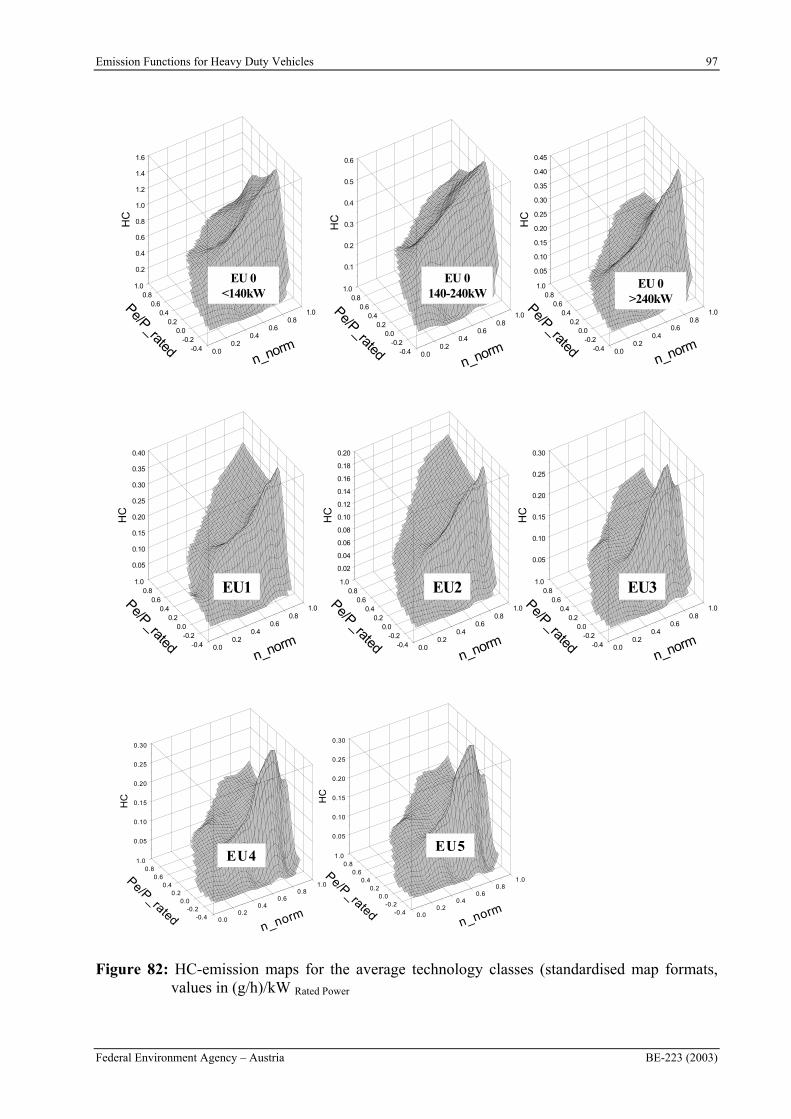
Emission Functions for Heavy Duty Vehicles 97
Federal Environment Agency – Austria BE-223 (2003)
-0.4-0.2
0.00.2
0.40.6
0.81.0
Pe/P_rated 0.00.2
0.40.6
0.81.0
n_norm
0.1
0.2
0.3
0.4
0.5
0.6
HC
-0.4-0.2
0.00.2
0.40.6
0.81.0
Pe/P_rated 0.00.2
0.40.6
0.81.0
n_norm
0.2
0.4
0.6
0.8
1.0
1.2
1.4
1.6
HC
-0.4-0.2
0.00.2
0.40.6
0.81.0
Pe/P_rated 0.00.2
0.40.6
0.81.0
n_norm
0.05
0.10
0.15
0.20
0.25
0.30
0.35
0.40
0.45
HC
EU 0140-240kW
EU 0<140kW
EU 0>240kW
-0.4-0.2
0.00.2
0.40.6
0.81.0
Pe/P_rated 0.00.2
0.40.6
0.81.0
n_norm
0.05
0.10
0.15
0.20
0.25
0.30
HC
EU3
-0.4-0.2
0.00.2
0.40.6
0.81.0
Pe/P_rated 0.00.2
0.40.6
0.81.0
n_norm
0.02
0.04
0.06
0.08
0.10
0.12
0.14
0.16
0.18
0.20
HC
EU2
-0.4-0.2
0.00.2
0.40.6
0.81.0
Pe/P_rated 0.00.2
0.40.6
0.81.0
n_norm
0.05
0.10
0.15
0.20
0.25
0.30
0.35
0.40
HC
EU1
-0.4-0.2
0.00.2
0.40.6
0.81.0
Pe/P_rated 0.00.2
0.40.6
0.81.0
n_norm
0.05
0.10
0.15
0.20
0.25
0.30
HC
-0.4-0.2
0.00.2
0.40.6
0.81.0
Pe/P_rated 0.00.2
0.40.6
0.81.0
n_norm
0.05
0.10
0.15
0.20
0.25
0.30
HC
EU4EU5
Figure 82: HC-emission maps for the average technology classes (standardised map formats, values in (g/h)/kW Rated Power
98 Emission Functions for Heavy Duty Vehicles
BE-223 (2003) Federal Environment Agency – Austria
7 CALCULATION OF THE EMISSION FACTORS
With the model PHEM a new set of emission factors for the Handbook of Emission Factors was calculated. For the simulation runs the engine maps according to chapter 6.3 and the transient correction functions according to chapter 5.4.2 have been used. The emission functions had to be delivered for several different HDV categories (Table 22). The categories were defined by the D.A.CH consortium and show slight changes compared to the categories used so far in the handbook (HBEFA 1.2).
For all HDV categories, all EURO classes and all driving cycles established in the Handbook all sensible combinations of vehicle loading (0%, 50%, 100%) and road gradients (-6%, -4%, -2%, 0%, 2%, 4%, 6%) have been calculated. In total this resulted in more than 30.000 combinations where emission factors are delivered. The results will be introduced by INFRAS-Schweiz in the Handbook Emissions Factors to allow a user- friendly handling of the huge amount of data. The following describes the most relevant model input data and summarises some of the results.
7.1 Vehicle data
For each of the basic HDV categories emission factors for the technology classes “pre EURO 1” up to “EURO 5” were calculated. Unfortunately, the vehicle data used in the former version of the Handbook on Emissions Factors (Hassel, 1995) was not defined in any document. Thus, a new set of data had to be elaborated for the HDV categories (Table 22). The main technical features for HDV have been assessed from the following sources:
(a) vehicle mass, maximum allowed gross weight, engine rated power
For all HDV below 32 tons maximum allowed gross weight this data is drawn out of national registration data in Switzerland. For Germany and Austria no adequate statistical data is available. Data for trucks, truck trailers and semi trailers above 32t maximum allowed gross weight was elaborated from “Lastauto & Omnibus Journal” (different yearbooks) and specifications of the manufacturers.
(b) gross frontal area
The frontal area of HDV can vary significantly according to the driver’s cab category, where often several options are available for a given basic truck configuration. Even more influence on the frontal area is resulting from the type of bodywork (platform, box body,…), especially for smaller HDV where the bodywork most often has a much higher frontal area than the drivers cab.
For none of the countries involved into the D.A.CH cooperation the statistics on the HDV registration gives any information on the bodyworks of the vehicles. Thus the frontal areas given in Table 22 result from an estimation on the share of different bodyworks and the manufacturers specifications on the dimensions of their HDV.
(c) Drag coefficients (Cd-values)
The sources of drag for HDV are: front pressure, rear pressure, cab-trailer gap, underbody and skin friction. The drag coefficient thus is depending on the design of the vehicle category (solo truck, truck trailer,…), the driver’s cab, the bodywork, the underbody, etc.. As already mentioned in (b), no statistical data is available on the share of different bodyworks and driver’s cabs on the road. As for the frontal area also the drag coefficients of the HDV categories had to be estimated based on a data base. The data base includes manufacturer specifications and literature review (Huncho, 1998), (Nakamura, 2002), (Saltzman, 1999).
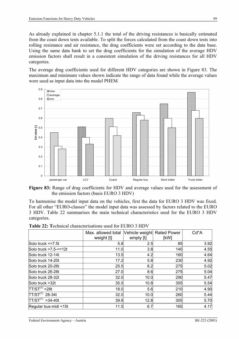
Emission Functions for Heavy Duty Vehicles 99
Federal Environment Agency – Austria BE-223 (2003)
As already explained in chapter 5.1.1 the total of the driving resistances is basically estimated from the coast down tests available. To split the forces calculated from the coast down tests into rolling resistance and air resistance, the drag coefficients were set according to the data base. Using the same data bank to set the drag coefficients for the simulation of the average HDV emission factors shall result in a consistent simulation of the driving resistances for all HDV categories.
The average drag coefficients used for different HDV categories are shown in Figure 83. The maximum and minimum values shown indicate the range of data found while the average values were used as input data into the model PHEM.
0
0.1
0.2
0.3
0.4
0.5
0.6
0.7
0.8
0.9
passenger car LCV Coach Regular bus Semi trailer Truck trailer
Cd
val
ue
[-]
max
average
min
Figure 83: Range of drag coefficients for HDV and average values used for the assessment of the emission factors (basis EURO 3 HDV)
To harmonise the model input data on the vehicles, first the data for EURO 3 HDV was fixed. For all other “EURO-classes” the model input data was assessed by factors related to the EURO 3 HDV. Table 22 summarises the main technical characteristics used for the EURO 3 HDV categories.
Table 22: Technical characterisations used for EURO 3 HDVMax. allowed total
weight [t] Vehicle weight
empty [t] Rated Power
[kW]Cd*A
Solo truck <=7.5t 5.8 2.5 85 3.92
Solo truck >7,5-<=12t 11.0 3.8 140 4.55
Solo truck 12-14t 13.5 4.2 160 4.64
Solo truck 14-20t 17.2 5.8 230 4.92
Solo truck 20-26t 25.5 8.2 275 5.02
Solo truck 26-28t 27.0 8.6 275 5.04
Solo truck 28-32t 32.0 10.0 290 5.47
Solo truck >32t 35.5 10.8 305 5.54
TT/ST(1) <28t 18.0 5.6 210 4.90TT/ST(1) 28-34t 32.0 10.0 260 5.44
TT/ST(1) >34-40t 39.8 12.8 305 5.70
Regular bus-midi <15t 11.5 6.7 165 4.17
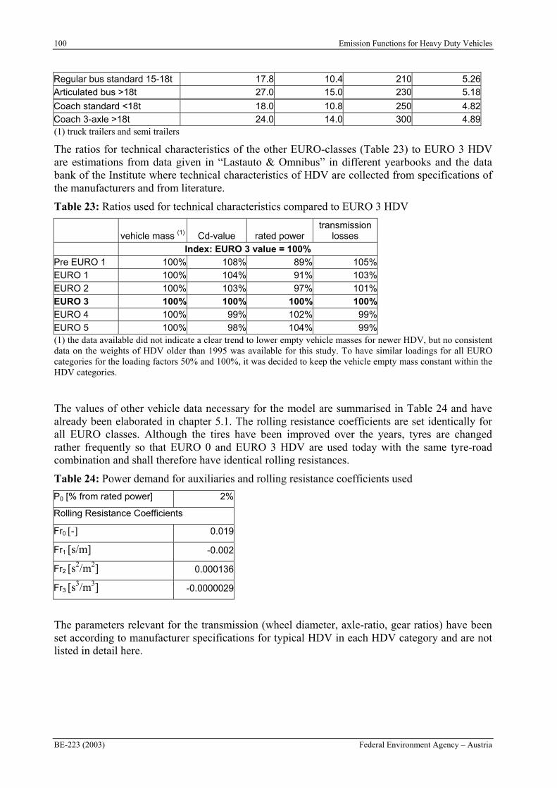
100 Emission Functions for Heavy Duty Vehicles
BE-223 (2003) Federal Environment Agency – Austria
Regular bus standard 15-18t 17.8 10.4 210 5.26
Articulated bus >18t 27.0 15.0 230 5.18
Coach standard <18t 18.0 10.8 250 4.82
Coach 3-axle >18t 24.0 14.0 300 4.89(1) truck trailers and semi trailers
The ratios for technical characteristics of the other EURO-classes (Table 23) to EURO 3 HDV are estimations from data given in “Lastauto & Omnibus” in different yearbooks and the data bank of the Institute where technical characteristics of HDV are collected from specifications of the manufacturers and from literature.
Table 23: Ratios used for technical characteristics compared to EURO 3 HDV
vehicle mass (1) Cd-value rated power transmission
losses
Index: EURO 3 value = 100% Pre EURO 1 100% 108% 89% 105%
EURO 1 100% 104% 91% 103%
EURO 2 100% 103% 97% 101%
EURO 3 100% 100% 100% 100%EURO 4 100% 99% 102% 99%
EURO 5 100% 98% 104% 99%(1) the data available did not indicate a clear trend to lower empty vehicle masses for newer HDV, but no consistent data on the weights of HDV older than 1995 was available for this study. To have similar loadings for all EURO categories for the loading factors 50% and 100%, it was decided to keep the vehicle empty mass constant within the HDV categories.
The values of other vehicle data necessary for the model are summarised in Table 24 and have already been elaborated in chapter 5.1. The rolling resistance coefficients are set identically for all EURO classes. Although the tires have been improved over the years, tyres are changed rather frequently so that EURO 0 and EURO 3 HDV are used today with the same tyre-road combination and shall therefore have identical rolling resistances.
Table 24: Power demand for auxiliaries and rolling resistance coefficients used
P0 [% from rated power] 2%
Rolling Resistance Coefficients
Fr0 [-] 0.019
Fr1 [s/m] -0.002
Fr2 [s2/m2] 0.000136
Fr3 [s3/m3] -0.0000029
The parameters relevant for the transmission (wheel diameter, axle-ratio, gear ratios) have been set according to manufacturer specifications for typical HDV in each HDV category and are not listed in detail here.
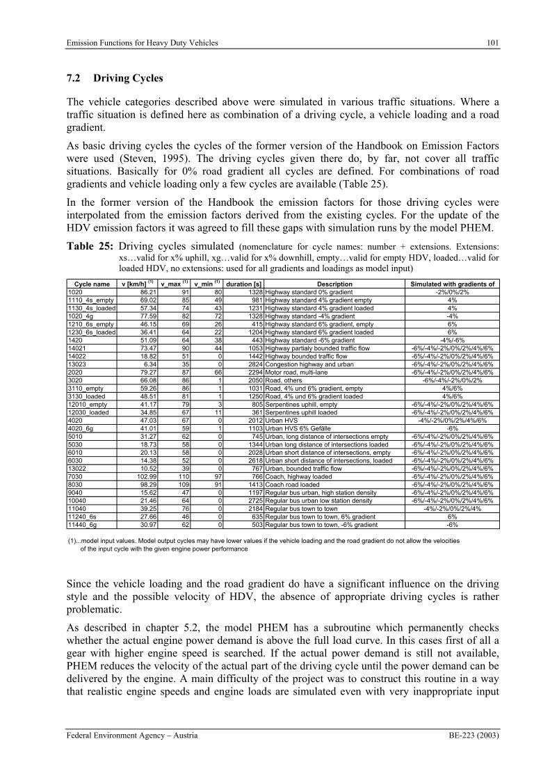
Emission Functions for Heavy Duty Vehicles 101
Federal Environment Agency – Austria BE-223 (2003)
7.2 Driving Cycles
The vehicle categories described above were simulated in various traffic situations. Where a traffic situation is defined here as combination of a driving cycle, a vehicle loading and a road gradient.
As basic driving cycles the cycles of the former version of the Handbook on Emission Factors were used (Steven, 1995). The driving cycles given there do, by far, not cover all traffic situations. Basically for 0% road gradient all cycles are defined. For combinations of road gradients and vehicle loading only a few cycles are available (Table 25).
In the former version of the Handbook the emission factors for those driving cycles were interpolated from the emission factors derived from the existing cycles. For the update of the HDV emission factors it was agreed to fill these gaps with simulation runs by the model PHEM.
Table 25: Driving cycles simulated (nomenclature for cycle names: number + extensions. Extensions: xs…valid for x% uphill, xg…valid for x% downhill, empty…valid for empty HDV, loaded…valid for loaded HDV, no extensions: used for all gradients and loadings as model input)
Cycle name v [km/h] (1) v_max (1) v_min (1) duration [s] Description Simulated with gradients of1020 86.21 91 80 1328 Highway standard 0% gradient -2%/0%/2%1110_4s_empty 69.02 85 49 981 Highway standard 4% gradient empty 4%1130_4s_loaded 57.34 74 43 1231 Highway standard 4% gradient loaded 4%1020_4g 77.59 82 72 1328 Highway standard -4% gradient -4%1210_6s_empty 46.15 69 26 415 Highway standard 6% gradient, empty 6%1230_6s_loaded 36.41 64 22 1204 Highway standard 6% gradient loaded 6%1420 51.09 64 38 443 Highway standard -6% gradient -4%/-6%14021 73.47 90 44 1053 Highway partialy bounded traffic flow -6%/-4%/-2%/0%/2%/4%/6%14022 18.82 51 0 1442 Highway bounded traffic flow -6%/-4%/-2%/0%/2%/4%/6%13023 6.34 35 0 2824 Congestion highway and urban -6%/-4%/-2%/0%/2%/4%/6%2020 79.27 87 66 2294 Motor road, multi-lane -6%/-4%/-2%/0%/2%/4%/6%3020 66.08 86 1 2050 Road, others -6%/-4%/-2%/0%/2%3110_empty 59.26 86 1 1031 Road, 4% und 6% gradient, empty 4%/6%3130_loaded 48.51 81 1 1250 Road, 4% und 6% gradient loaded 4%/6%12010_empty 41.17 79 3 805 Serpentines uphill, empty -6%/-4%/-2%/0%/2%/4%/6%12030_loaded 34.85 67 11 361 Serpentines uphill loaded -6%/-4%/-2%/0%/2%/4%/6%4020 47.03 67 0 2012 Urban HVS -4%/-2%/0%/2%/4%/6%4020_6g 41.01 59 1 1103 Urban HVS 6% Gefälle -6%5010 31.27 62 0 745 Urban, long distance of intersections empty -6%/-4%/-2%/0%/2%/4%/6%5030 18.73 58 0 1344 Urban long distance of intersections loaded -6%/-4%/-2%/0%/2%/4%/6%6010 20.13 58 0 2028 Urban short distance of intersections, empty -6%/-4%/-2%/0%/2%/4%/6%6030 14.38 52 0 2618 Urban short distance of intersections, loaded -6%/-4%/-2%/0%/2%/4%/6%13022 10.52 39 0 767 Urban, bounded traffic flow -6%/-4%/-2%/0%/2%/4%/6%7030 102.99 110 97 766 Coach, highway loaded -6%/-4%/-2%/0%/2%/4%/6%8030 98.29 109 91 1413 Coach road loaded -6%/-4%/-2%/0%/2%/4%/6%9040 15.62 47 0 1197 Regular bus urban, high station density -6%/-4%/-2%/0%/2%/4%/6%10040 21.46 64 0 2725 Regular bus urban low station density -6%/-4%/-2%/0%/2%/4%/6%11040 39.25 76 0 2184 Regular bus town to town -4%/-2%/0%/2%/4%11240_6s 27.66 46 0 635 Regular bus town to town, 6% gradient 6%11440_6g 30.97 62 0 503 Regular bus town to town, -6% gradient -6%
(1)...model input values. Model output cycles may have lower values if the vehicle loading and the road gradient do not allow the velocities of the input cycle with the given engine power performance
Since the vehicle loading and the road gradient do have a significant influence on the driving style and the possible velocity of HDV, the absence of appropriate driving cycles is rather problematic.
As described in chapter 5.2, the model PHEM has a subroutine which permanently checks whether the actual engine power demand is above the full load curve. In this cases first of all a gear with higher engine speed is searched. If the actual power demand is still not available, PHEM reduces the velocity of the actual part of the driving cycle until the power demand can be delivered by the engine. A main difficulty of the project was to construct this routine in a way that realistic engine speeds and engine loads are simulated even with very inappropriate input
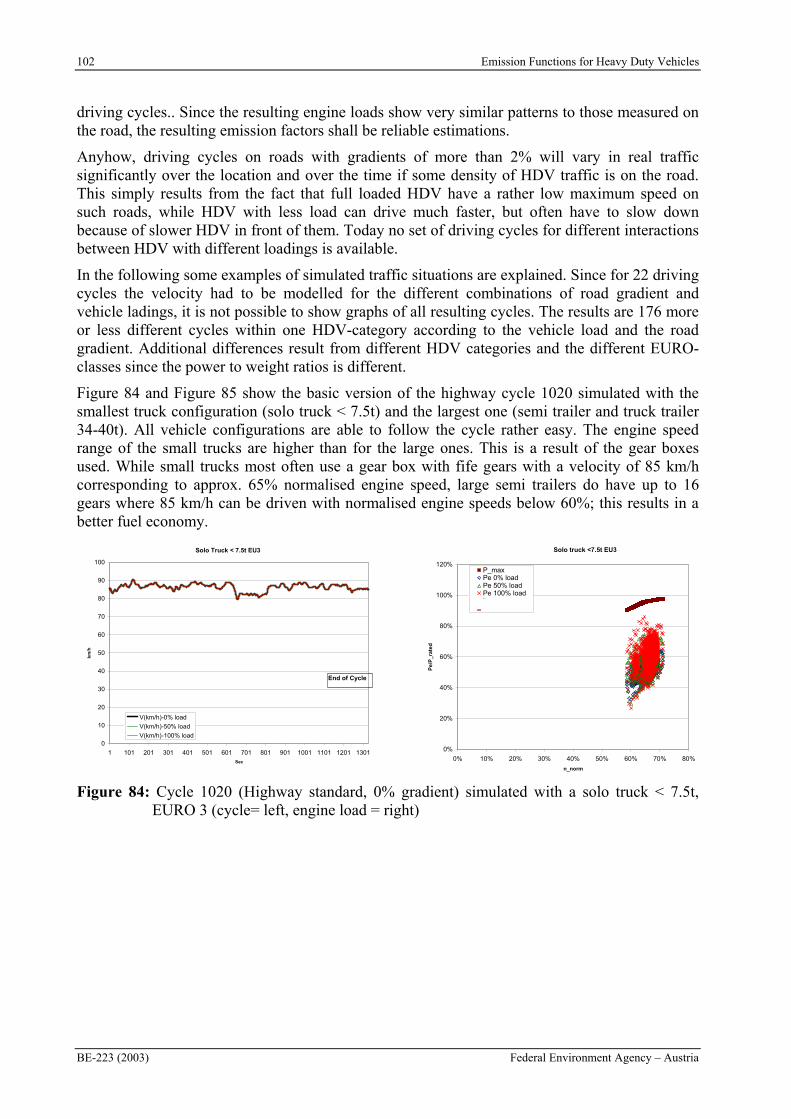
102 Emission Functions for Heavy Duty Vehicles
BE-223 (2003) Federal Environment Agency – Austria
driving cycles.. Since the resulting engine loads show very similar patterns to those measured on the road, the resulting emission factors shall be reliable estimations.
Anyhow, driving cycles on roads with gradients of more than 2% will vary in real traffic significantly over the location and over the time if some density of HDV traffic is on the road. This simply results from the fact that full loaded HDV have a rather low maximum speed on such roads, while HDV with less load can drive much faster, but often have to slow down because of slower HDV in front of them. Today no set of driving cycles for different interactions between HDV with different loadings is available.
In the following some examples of simulated traffic situations are explained. Since for 22 driving cycles the velocity had to be modelled for the different combinations of road gradient and vehicle ladings, it is not possible to show graphs of all resulting cycles. The results are 176 more or less different cycles within one HDV-category according to the vehicle load and the road gradient. Additional differences result from different HDV categories and the different EURO-classes since the power to weight ratios is different.
Figure 84 and Figure 85 show the basic version of the highway cycle 1020 simulated with the smallest truck configuration (solo truck < 7.5t) and the largest one (semi trailer and truck trailer 34-40t). All vehicle configurations are able to follow the cycle rather easy. The engine speed range of the small trucks are higher than for the large ones. This is a result of the gear boxes used. While small trucks most often use a gear box with fife gears with a velocity of 85 km/h corresponding to approx. 65% normalised engine speed, large semi trailers do have up to 16 gears where 85 km/h can be driven with normalised engine speeds below 60%; this results in a better fuel economy.
Solo Truck < 7.5t EU3
0
10
20
30
40
50
60
70
80
90
100
1 101 201 301 401 501 601 701 801 901 1001 1101 1201 1301Sec
km/h
V(km/h)-0% load
V(km/h)-50% load
V(km/h)-100% load
End of Cycle
Solo truck <7.5t EU3
0%
20%
40%
60%
80%
100%
120%
0% 10% 20% 30% 40% 50% 60% 70% 80%
n_norm
Pe/
P_r
ated
P_maxPe 0% loadPe 50% loadPe 100% load''''
Figure 84: Cycle 1020 (Highway standard, 0% gradient) simulated with a solo truck < 7.5t, EURO 3 (cycle= left, engine load = right)
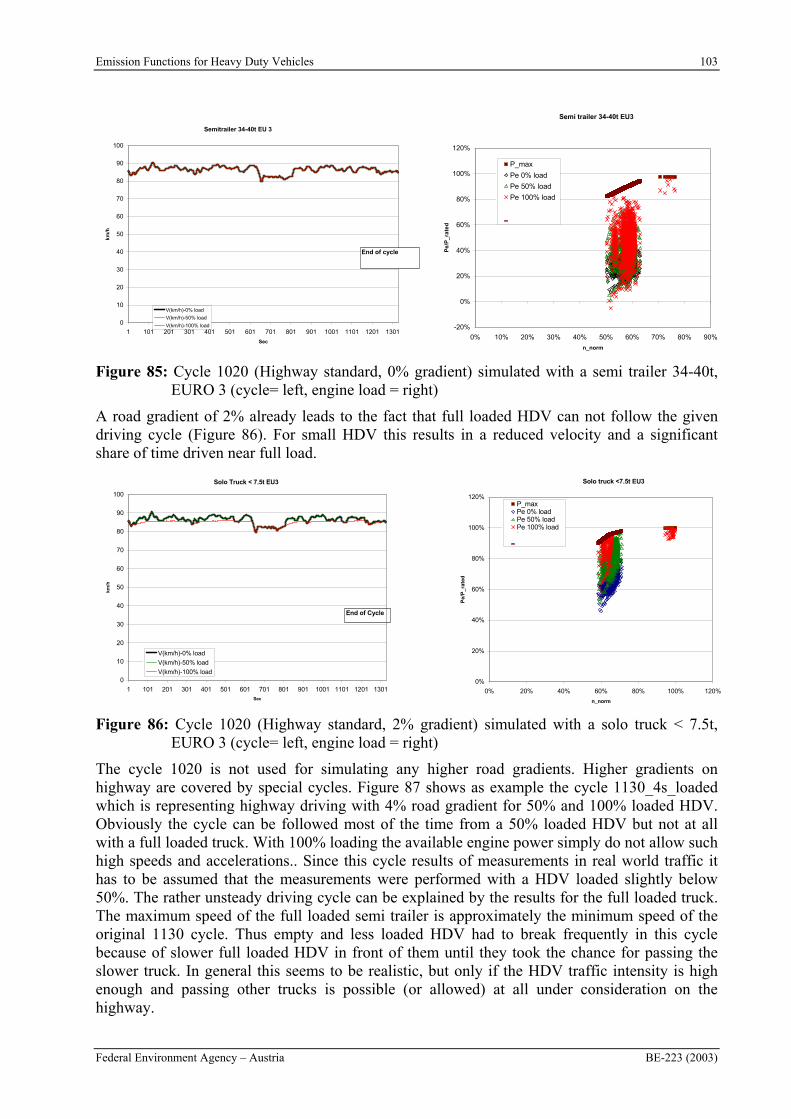
Emission Functions for Heavy Duty Vehicles 103
Federal Environment Agency – Austria BE-223 (2003)
Semitrailer 34-40t EU 3
0
10
20
30
40
50
60
70
80
90
100
1 101 201 301 401 501 601 701 801 901 1001 1101 1201 1301
Sec
km/h
V(km/h)-0% load
V(km/h)-50% load
V(km/h)-100% load
End of cycle
Semi trailer 34-40t EU3
-20%
0%
20%
40%
60%
80%
100%
120%
0% 10% 20% 30% 40% 50% 60% 70% 80% 90%
n_norm
Pe
/P_
rate
d
P_max
Pe 0% load
Pe 50% load
Pe 100% load
''
''
Figure 85: Cycle 1020 (Highway standard, 0% gradient) simulated with a semi trailer 34-40t, EURO 3 (cycle= left, engine load = right)
A road gradient of 2% already leads to the fact that full loaded HDV can not follow the given driving cycle (Figure 86). For small HDV this results in a reduced velocity and a significant share of time driven near full load.
Solo Truck < 7.5t EU3
0
10
20
30
40
50
60
70
80
90
100
1 101 201 301 401 501 601 701 801 901 1001 1101 1201 1301Sec
km/h
V(km/h)-0% load
V(km/h)-50% load
V(km/h)-100% load
End of Cycle
Solo truck <7.5t EU3
0%
20%
40%
60%
80%
100%
120%
0% 20% 40% 60% 80% 100% 120%
n_norm
Pe/
P_r
ated
P_maxPe 0% loadPe 50% loadPe 100% load''''
Figure 86: Cycle 1020 (Highway standard, 2% gradient) simulated with a solo truck < 7.5t, EURO 3 (cycle= left, engine load = right)
The cycle 1020 is not used for simulating any higher road gradients. Higher gradients on highway are covered by special cycles. Figure 87 shows as example the cycle 1130_4s_loaded which is representing highway driving with 4% road gradient for 50% and 100% loaded HDV. Obviously the cycle can be followed most of the time from a 50% loaded HDV but not at all with a full loaded truck. With 100% loading the available engine power simply do not allow such high speeds and accelerations.. Since this cycle results of measurements in real world traffic it has to be assumed that the measurements were performed with a HDV loaded slightly below 50%. The rather unsteady driving cycle can be explained by the results for the full loaded truck. The maximum speed of the full loaded semi trailer is approximately the minimum speed of the original 1130 cycle. Thus empty and less loaded HDV had to break frequently in this cycle because of slower full loaded HDV in front of them until they took the chance for passing the slower truck. In general this seems to be realistic, but only if the HDV traffic intensity is high enough and passing other trucks is possible (or allowed) at all under consideration on the highway.
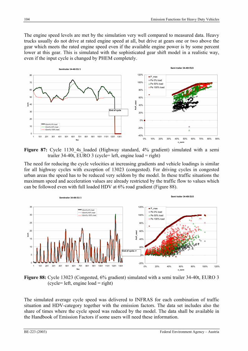
104 Emission Functions for Heavy Duty Vehicles
BE-223 (2003) Federal Environment Agency – Austria
The engine speed levels are met by the simulation very well compared to measured data. Heavy trucks usually do not drive at rated engine speed at all, but drive at gears one or two above the gear which meets the rated engine speed even if the available engine power is by some percent lower at this gear. This is simulated with the sophisticated gear shift model in a realistic way, even if the input cycle is changed by PHEM completely.
Semitrailer 34-40t EU 3
0
10
20
30
40
50
60
70
80
1 101 201 301 401 501 601 701 801 901 1001 1101 1201 1301
Sec
km/h
V(km/h)-0% load
V(km/h)-50% load
V(km/h)-100% load
End of cycle
Semi trailer 34-40t EU3
-40%
-20%
0%
20%
40%
60%
80%
100%
120%
0% 10% 20% 30% 40% 50% 60% 70% 80% 90%
n_norm
Pe/
P_r
ated
P_max
Pe 0% load
Pe 50% load
Pe 100% load
''
''
Figure 87: Cycle 1130_4s_loaded (Highway standard, 4% gradient) simulated with a semi trailer 34-40t, EURO 3 (cycle= left, engine load = right)
The need for reducing the cycle velocities at increasing gradients and vehicle loadings is similar for all highway cycles with exception of 13023 (congested). For driving cycles in congested urban areas the speed has to be reduced very seldom by the model. In these traffic situations the maximum speed and acceleration values are already restricted by the traffic flow to values which can be followed even with full loaded HDV at 6% road gradient (Figure 88).
Semitrailer 34-40t EU 3
0
5
10
15
20
25
30
35
1 101 201 301 401 501 601 701 801 901 1001 1101 1201 1301
Sec
km
/h
V(km/h)-0% load
V(km/h)-50% load
V(km/h)-100% load
End of cycle-->
Semi trailer 34-40t EU3
-20%
0%
20%
40%
60%
80%
100%
120%
0% 20% 40% 60% 80% 100% 120%
n_norm
Pe/
P_r
ated
P_max
Pe 0% load
Pe 50% load
Pe 100% load
''
''
Figure 88: Cycle 13023 (Congested, 6% gradient) simulated with a semi trailer 34-40t, EURO 3 (cycle= left, engine load = right)
The simulated average cycle speed was delivered to INFRAS for each combination of traffic situation and HDV-category together with the emission factors. The data set includes also the share of times where the cycle speed was reduced by the model. The data shall be available in the Handbook of Emission Factors if some users will need these information.
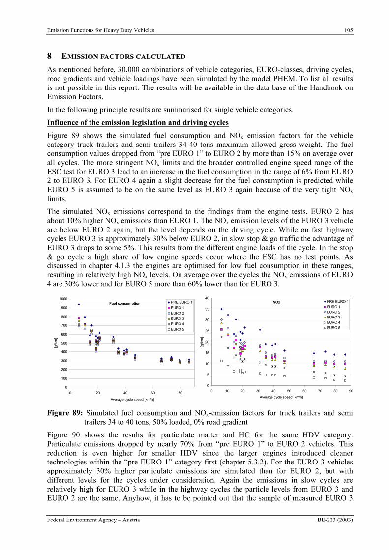
Emission Functions for Heavy Duty Vehicles 105
Federal Environment Agency – Austria BE-223 (2003)
8 EMISSION FACTORS CALCULATED
As mentioned before, 30.000 combinations of vehicle categories, EURO-classes, driving cycles, road gradients and vehicle loadings have been simulated by the model PHEM. To list all results is not possible in this report. The results will be available in the data base of the Handbook on Emission Factors.
In the following principle results are summarised for single vehicle categories.
Influence of the emission legislation and driving cycles
Figure 89 shows the simulated fuel consumption and NOx emission factors for the vehicle category truck trailers and semi trailers 34-40 tons maximum allowed gross weight. The fuel consumption values dropped from “pre EURO 1” to EURO 2 by more than 15% on average over all cycles. The more stringent NOx limits and the broader controlled engine speed range of the ESC test for EURO 3 lead to an increase in the fuel consumption in the range of 6% from EURO 2 to EURO 3. For EURO 4 again a slight decrease for the fuel consumption is predicted while EURO 5 is assumed to be on the same level as EURO 3 again because of the very tight NOx
limits.
The simulated NOx emissions correspond to the findings from the engine tests. EURO 2 has about 10% higher NOx emissions than EURO 1. The NOx emission levels of the EURO 3 vehicle are below EURO 2 again, but the level depends on the driving cycle. While on fast highway cycles EURO 3 is approximately 30% below EURO 2, in slow stop & go traffic the advantage of EURO 3 drops to some 5%. This results from the different engine loads of the cycle. In the stop & go cycle a high share of low engine speeds occur where the ESC has no test points. As discussed in chapter 4.1.3 the engines are optimised for low fuel consumption in these ranges, resulting in relatively high NOx levels. On average over the cycles the NOx emissions of EURO 4 are 30% lower and for EURO 5 more than 60% lower than for EURO 3.
0
100
200
300
400
500
600
700
800
900
1000
0 20 40 60 80
Average cycle speed [km/h]
[g/k
m]
PRE EURO 1
EURO 1
EURO 2
EURO 3
EURO 4
EURO 5
Fuel consumption
0
5
10
15
20
25
30
35
40
0 10 20 30 40 50 60 70 80 90
Average cycle speed [km/h]
[g/k
m]
PRE EURO 1EURO 1EURO 2EURO 3EURO 4EURO 5
NOx
Figure 89: Simulated fuel consumption and NOx-emission factors for truck trailers and semi trailers 34 to 40 tons, 50% loaded, 0% road gradient
Figure 90 shows the results for particulate matter and HC for the same HDV category. Particulate emissions dropped by nearly 70% from “pre EURO 1” to EURO 2 vehicles. This reduction is even higher for smaller HDV since the larger engines introduced cleaner technologies within the “pre EURO 1” category first (chapter 5.3.2). For the EURO 3 vehicles approximately 30% higher particulate emissions are simulated than for EURO 2, but with different levels for the cycles under consideration. Again the emissions in slow cycles are relatively high for EURO 3 while in the highway cycles the particle levels from EURO 3 and EURO 2 are the same. Anyhow, it has to be pointed out that the sample of measured EURO 3
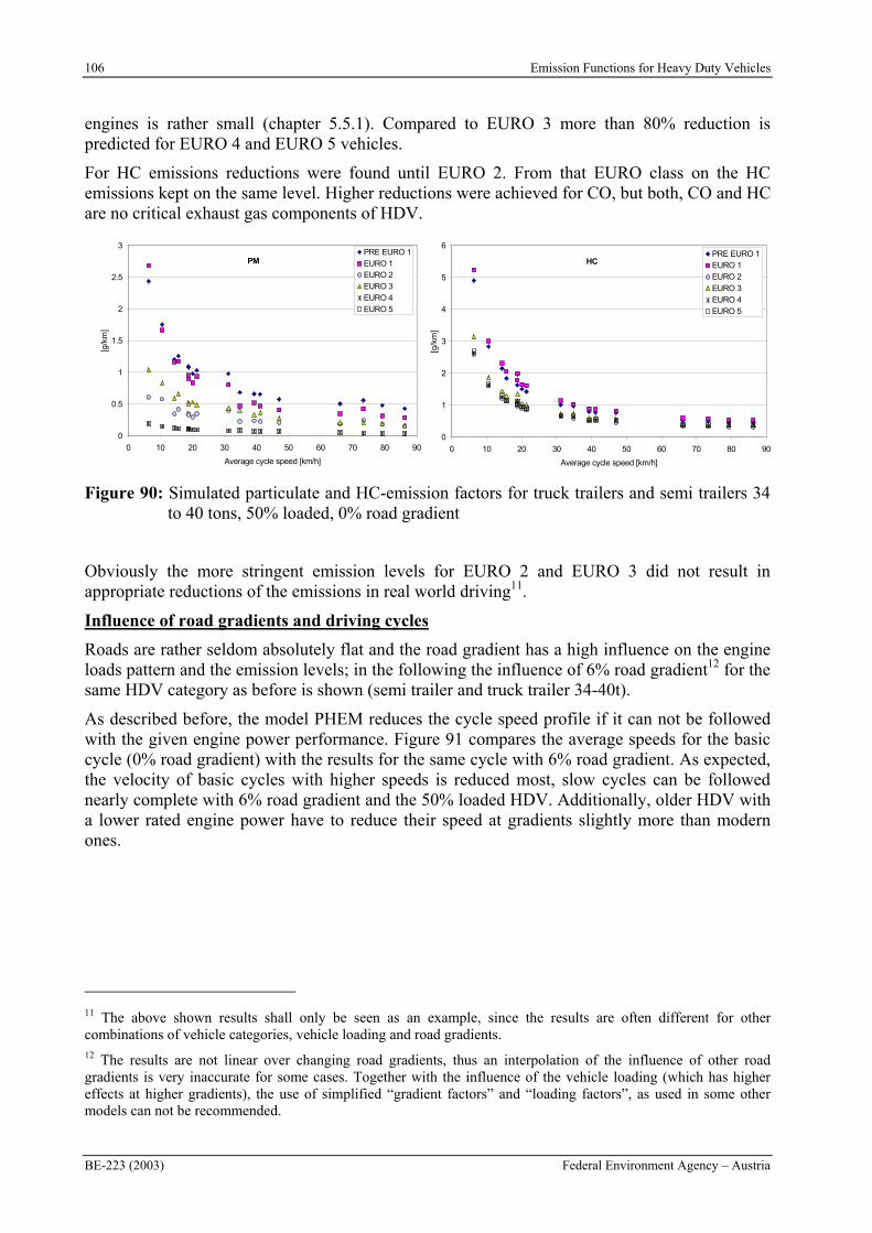
106 Emission Functions for Heavy Duty Vehicles
BE-223 (2003) Federal Environment Agency – Austria
engines is rather small (chapter 5.5.1). Compared to EURO 3 more than 80% reduction is predicted for EURO 4 and EURO 5 vehicles.
For HC emissions reductions were found until EURO 2. From that EURO class on the HC emissions kept on the same level. Higher reductions were achieved for CO, but both, CO and HC are no critical exhaust gas components of HDV.
0
0.5
1
1.5
2
2.5
3
0 10 20 30 40 50 60 70 80 90
Average cycle speed [km/h]
[g/k
m]
PRE EURO 1EURO 1EURO 2EURO 3EURO 4EURO 5
PM
0
1
2
3
4
5
6
0 10 20 30 40 50 60 70 80 90
Average cycle speed [km/h]
[g/k
m]
PRE EURO 1EURO 1EURO 2EURO 3EURO 4EURO 5
HC
Figure 90: Simulated particulate and HC-emission factors for truck trailers and semi trailers 34 to 40 tons, 50% loaded, 0% road gradient
Obviously the more stringent emission levels for EURO 2 and EURO 3 did not result in appropriate reductions of the emissions in real world driving11.
Influence of road gradients and driving cycles
Roads are rather seldom absolutely flat and the road gradient has a high influence on the engine loads pattern and the emission levels; in the following the influence of 6% road gradient12 for the same HDV category as before is shown (semi trailer and truck trailer 34-40t).
As described before, the model PHEM reduces the cycle speed profile if it can not be followed with the given engine power performance. Figure 91 compares the average speeds for the basic cycle (0% road gradient) with the results for the same cycle with 6% road gradient. As expected, the velocity of basic cycles with higher speeds is reduced most, slow cycles can be followed nearly complete with 6% road gradient and the 50% loaded HDV. Additionally, older HDV with a lower rated engine power have to reduce their speed at gradients slightly more than modern ones.
11 The above shown results shall only be seen as an example, since the results are often different for other combinations of vehicle categories, vehicle loading and road gradients. 12 The results are not linear over changing road gradients, thus an interpolation of the influence of other road gradients is very inaccurate for some cases. Together with the influence of the vehicle loading (which has higher effects at higher gradients), the use of simplified “gradient factors” and “loading factors”, as used in some other models can not be recommended.
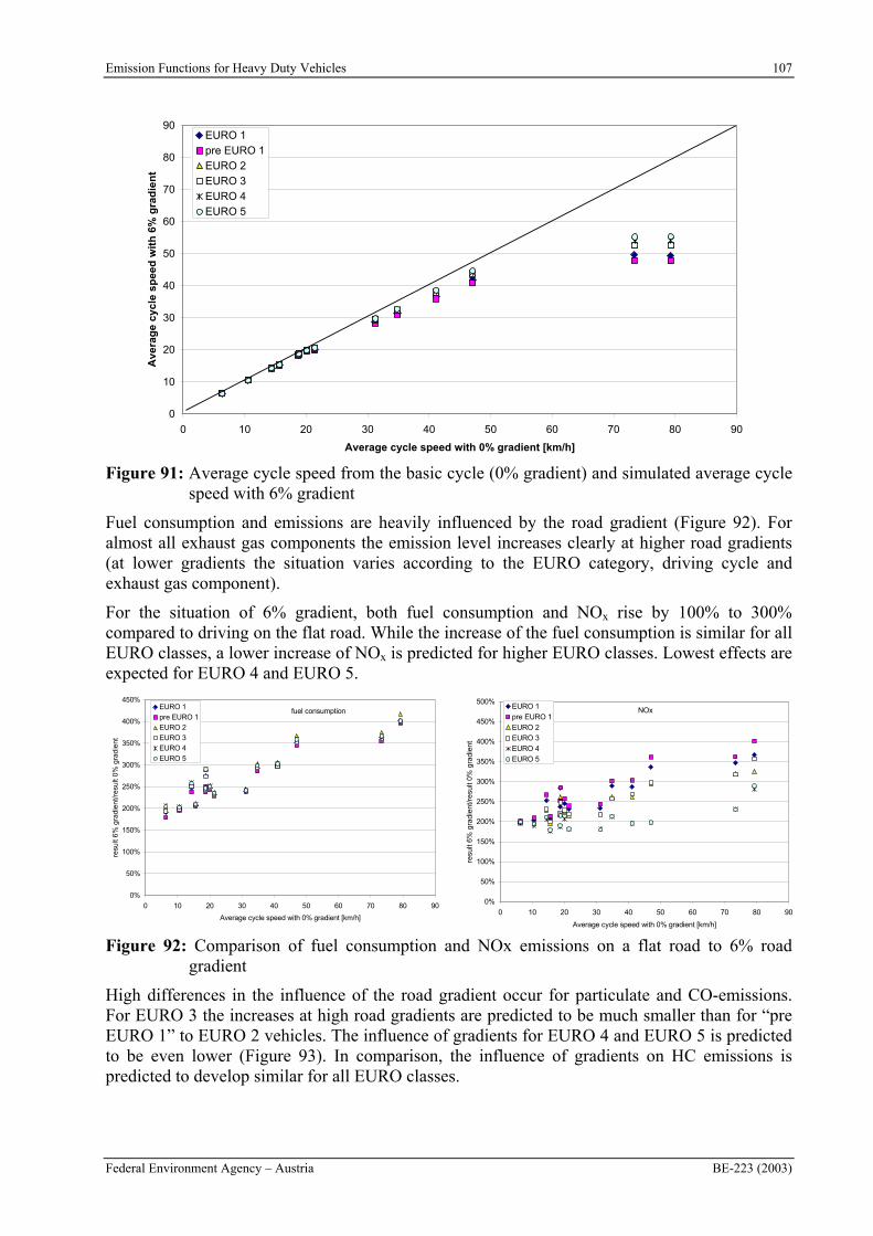
Emission Functions for Heavy Duty Vehicles 107
Federal Environment Agency – Austria BE-223 (2003)
0
10
20
30
40
50
60
70
80
90
0 10 20 30 40 50 60 70 80 90
Average cycle speed with 0% gradient [km/h]
Ave
rag
e cy
cle
spee
d w
ith
6%
gra
die
nt
EURO 1pre EURO 1EURO 2EURO 3EURO 4EURO 5
Figure 91: Average cycle speed from the basic cycle (0% gradient) and simulated average cycle speed with 6% gradient
Fuel consumption and emissions are heavily influenced by the road gradient (Figure 92). For almost all exhaust gas components the emission level increases clearly at higher road gradients (at lower gradients the situation varies according to the EURO category, driving cycle and exhaust gas component).
For the situation of 6% gradient, both fuel consumption and NOx rise by 100% to 300% compared to driving on the flat road. While the increase of the fuel consumption is similar for all EURO classes, a lower increase of NOx is predicted for higher EURO classes. Lowest effects are expected for EURO 4 and EURO 5.
fuel consumption
0%
50%
100%
150%
200%
250%
300%
350%
400%
450%
0 10 20 30 40 50 60 70 80 90
Average cycle speed with 0% gradient [km/h]
resu
lt 6%
gra
dien
t/re
sult
0% g
radi
ent
EURO 1pre EURO 1EURO 2EURO 3EURO 4
EURO 5
NOx
0%
50%
100%
150%
200%
250%
300%
350%
400%
450%
500%
0 10 20 30 40 50 60 70 80 90
Average cycle speed with 0% gradient [km/h]
resu
lt 6%
gra
dien
t/res
ult 0
% g
radi
ent
EURO 1
pre EURO 1
EURO 2EURO 3
EURO 4
EURO 5
Figure 92: Comparison of fuel consumption and NOx emissions on a flat road to 6% road gradient
High differences in the influence of the road gradient occur for particulate and CO-emissions. For EURO 3 the increases at high road gradients are predicted to be much smaller than for “pre EURO 1” to EURO 2 vehicles. The influence of gradients for EURO 4 and EURO 5 is predicted to be even lower (Figure 93). In comparison, the influence of gradients on HC emissions is predicted to develop similar for all EURO classes.
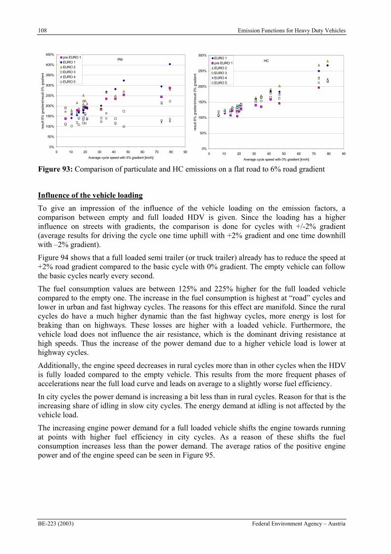
108 Emission Functions for Heavy Duty Vehicles
BE-223 (2003) Federal Environment Agency – Austria
PM
0%
50%
100%
150%
200%
250%
300%
350%
400%
450%
0 10 20 30 40 50 60 70 80 90
Average cycle speed with 0% gradient [km/h]
resu
lt 6%
gra
dien
t/res
ult 0
% g
radi
ent
pre EURO 1
EURO 1EURO 2
EURO 3
EURO 4EURO 5
HC
0%
50%
100%
150%
200%
250%
300%
0 10 20 30 40 50 60 70 80 90
Average cycle speed with 0% gradient [km/h]
resu
lt 6%
gra
dien
t/res
ult 0
% g
radi
ent
EURO 1
pre EURO 1
EURO 2
EURO 3EURO 4
EURO 5
Figure 93: Comparison of particulate and HC emissions on a flat road to 6% road gradient
Influence of the vehicle loading
To give an impression of the influence of the vehicle loading on the emission factors, a comparison between empty and full loaded HDV is given. Since the loading has a higher influence on streets with gradients, the comparison is done for cycles with +/-2% gradient (average results for driving the cycle one time uphill with +2% gradient and one time downhill with –2% gradient).
Figure 94 shows that a full loaded semi trailer (or truck trailer) already has to reduce the speed at +2% road gradient compared to the basic cycle with 0% gradient. The empty vehicle can follow the basic cycles nearly every second.
The fuel consumption values are between 125% and 225% higher for the full loaded vehicle compared to the empty one. The increase in the fuel consumption is highest at “road” cycles and lower in urban and fast highway cycles. The reasons for this effect are manifold. Since the rural cycles do have a much higher dynamic than the fast highway cycles, more energy is lost for braking than on highways. These losses are higher with a loaded vehicle. Furthermore, the vehicle load does not influence the air resistance, which is the dominant driving resistance at high speeds. Thus the increase of the power demand due to a higher vehicle load is lower at highway cycles.
Additionally, the engine speed decreases in rural cycles more than in other cycles when the HDV is fully loaded compared to the empty vehicle. This results from the more frequent phases of accelerations near the full load curve and leads on average to a slightly worse fuel efficiency.
In city cycles the power demand is increasing a bit less than in rural cycles. Reason for that is the increasing share of idling in slow city cycles. The energy demand at idling is not affected by the vehicle load.
The increasing engine power demand for a full loaded vehicle shifts the engine towards running at points with higher fuel efficiency in city cycles. As a reason of these shifts the fuel consumption increases less than the power demand. The average ratios of the positive engine power and of the engine speed can be seen in Figure 95.
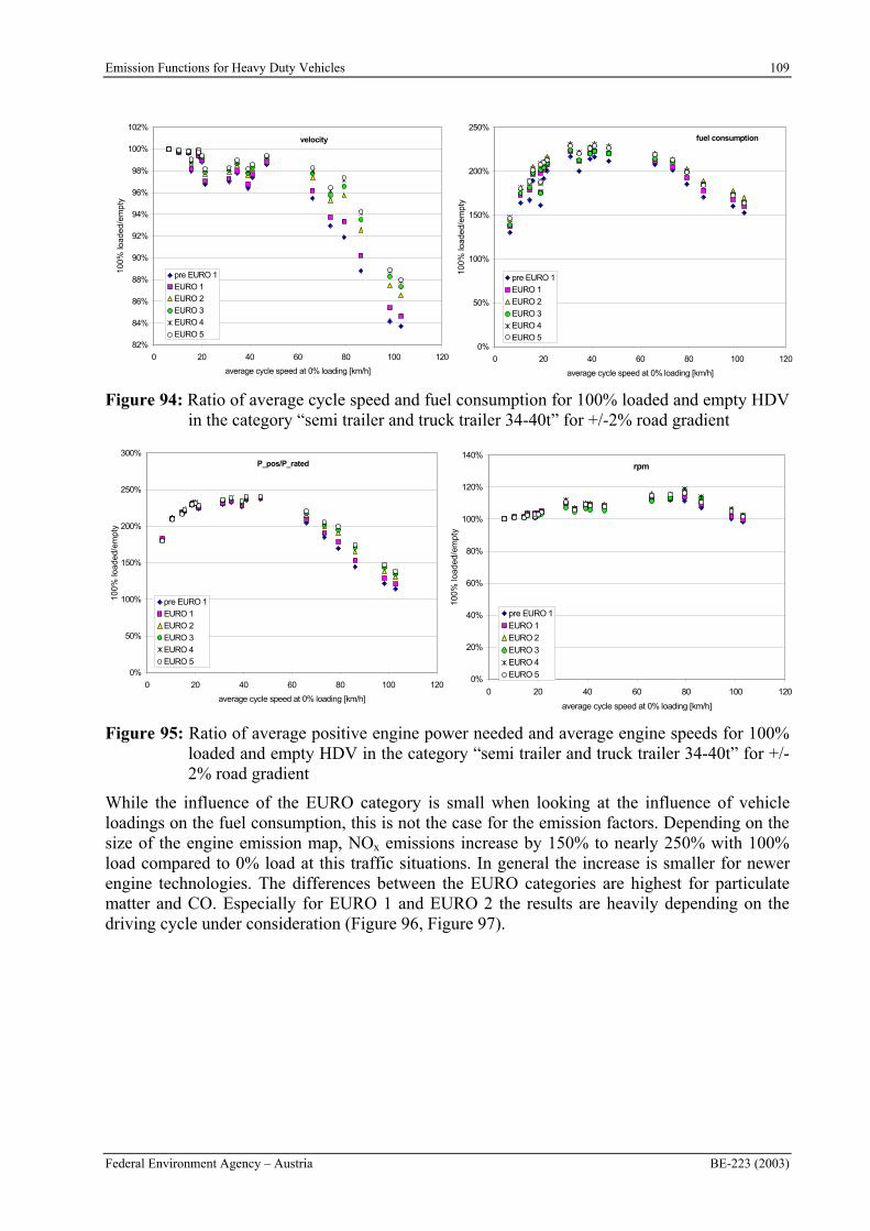
Emission Functions for Heavy Duty Vehicles 109
Federal Environment Agency – Austria BE-223 (2003)
82%
84%
86%
88%
90%
92%
94%
96%
98%
100%
102%
0 20 40 60 80 100 120
average cycle speed at 0% loading [km/h]
10
0%
loa
de
d/e
mp
ty
pre EURO 1
EURO 1
EURO 2
EURO 3
EURO 4
EURO 5
velocity
0%
50%
100%
150%
200%
250%
0 20 40 60 80 100 120
average cycle speed at 0% loading [km/h]
100%
load
ed/e
mpt
y
pre EURO 1
EURO 1
EURO 2
EURO 3
EURO 4
EURO 5
fuel consumption
Figure 94: Ratio of average cycle speed and fuel consumption for 100% loaded and empty HDV in the category “semi trailer and truck trailer 34-40t” for +/-2% road gradient
0%
50%
100%
150%
200%
250%
300%
0 20 40 60 80 100 120
average cycle speed at 0% loading [km/h]
100%
load
ed/e
mpt
y
pre EURO 1
EURO 1
EURO 2
EURO 3
EURO 4
EURO 5
P_pos/P_rated
0%
20%
40%
60%
80%
100%
120%
140%
0 20 40 60 80 100 120
average cycle speed at 0% loading [km/h]
100%
load
ed/e
mpt
y
pre EURO 1
EURO 1
EURO 2
EURO 3
EURO 4
EURO 5
rpm
Figure 95: Ratio of average positive engine power needed and average engine speeds for 100% loaded and empty HDV in the category “semi trailer and truck trailer 34-40t” for +/-2% road gradient
While the influence of the EURO category is small when looking at the influence of vehicle loadings on the fuel consumption, this is not the case for the emission factors. Depending on the size of the engine emission map, NOx emissions increase by 150% to nearly 250% with 100% load compared to 0% load at this traffic situations. In general the increase is smaller for newer engine technologies. The differences between the EURO categories are highest for particulate matter and CO. Especially for EURO 1 and EURO 2 the results are heavily depending on the driving cycle under consideration (Figure 96, Figure 97).
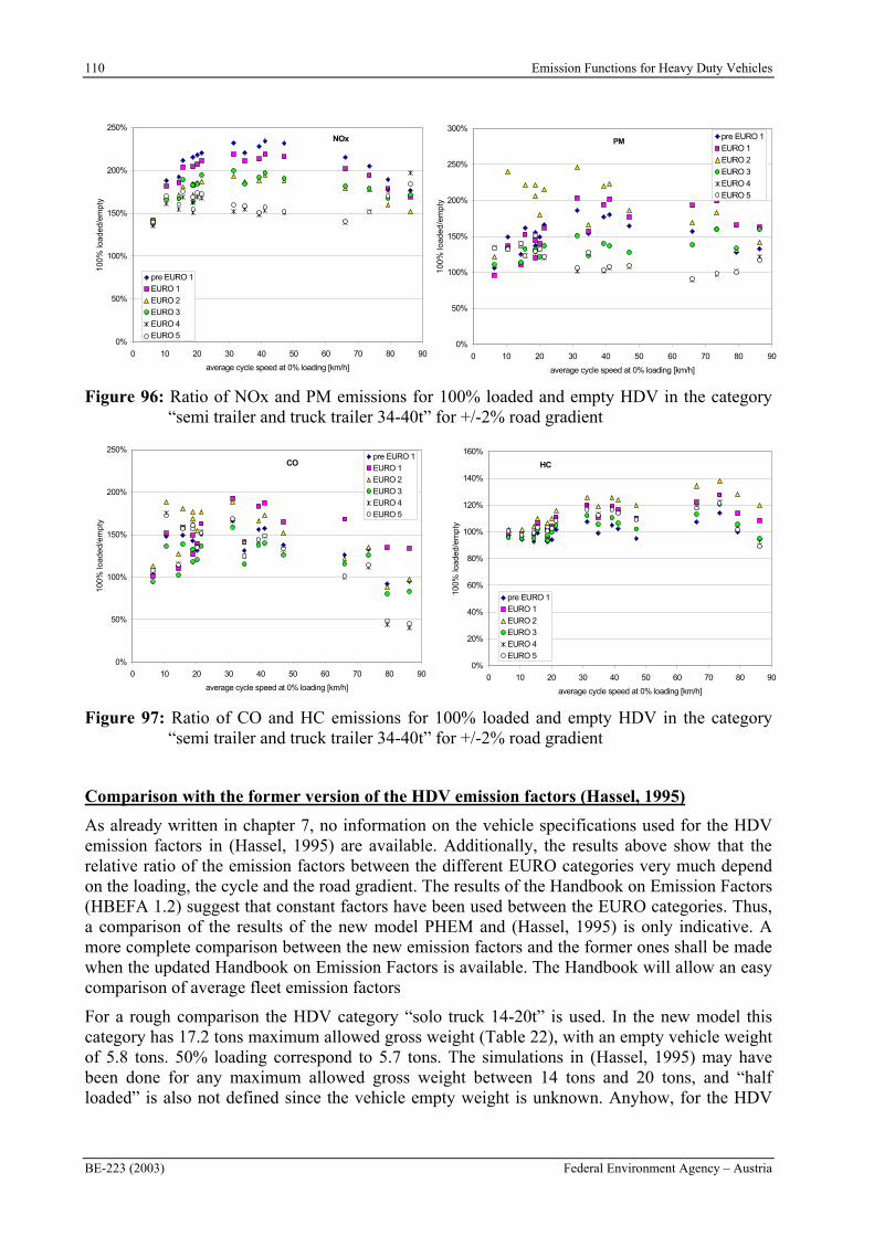
110 Emission Functions for Heavy Duty Vehicles
BE-223 (2003) Federal Environment Agency – Austria
0%
50%
100%
150%
200%
250%
300%
0 10 20 30 40 50 60 70 80 90
average cycle speed at 0% loading [km/h]
100%
load
ed/e
mpt
y
pre EURO 1
EURO 1
EURO 2
EURO 3
EURO 4
EURO 5
PM
0%
50%
100%
150%
200%
250%
0 10 20 30 40 50 60 70 80 90
average cycle speed at 0% loading [km/h]
100%
load
ed/e
mpt
y
pre EURO 1
EURO 1
EURO 2
EURO 3
EURO 4
EURO 5
NOx
Figure 96: Ratio of NOx and PM emissions for 100% loaded and empty HDV in the category “semi trailer and truck trailer 34-40t” for +/-2% road gradient
0%
50%
100%
150%
200%
250%
0 10 20 30 40 50 60 70 80 90
average cycle speed at 0% loading [km/h]
100%
load
ed/e
mpt
y
pre EURO 1
EURO 1
EURO 2
EURO 3
EURO 4
EURO 5
CO
0%
20%
40%
60%
80%
100%
120%
140%
160%
0 10 20 30 40 50 60 70 80 90
average cycle speed at 0% loading [km/h]
100%
load
ed/e
mpt
y
pre EURO 1
EURO 1
EURO 2
EURO 3
EURO 4
EURO 5
HC
Figure 97: Ratio of CO and HC emissions for 100% loaded and empty HDV in the category “semi trailer and truck trailer 34-40t” for +/-2% road gradient
Comparison with the former version of the HDV emission factors (Hassel, 1995)
As already written in chapter 7, no information on the vehicle specifications used for the HDV emission factors in (Hassel, 1995) are available. Additionally, the results above show that the relative ratio of the emission factors between the different EURO categories very much depend on the loading, the cycle and the road gradient. The results of the Handbook on Emission Factors (HBEFA 1.2) suggest that constant factors have been used between the EURO categories. Thus, a comparison of the results of the new model PHEM and (Hassel, 1995) is only indicative. A more complete comparison between the new emission factors and the former ones shall be made when the updated Handbook on Emission Factors is available. The Handbook will allow an easy comparison of average fleet emission factors
For a rough comparison the HDV category “solo truck 14-20t” is used. In the new model this category has 17.2 tons maximum allowed gross weight (Table 22), with an empty vehicle weight of 5.8 tons. 50% loading correspond to 5.7 tons. The simulations in (Hassel, 1995) may have been done for any maximum allowed gross weight between 14 tons and 20 tons, and “half loaded” is also not defined since the vehicle empty weight is unknown. Anyhow, for the HDV
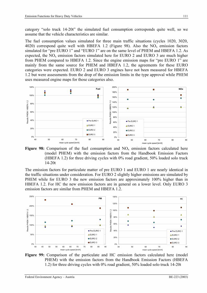
Emission Functions for Heavy Duty Vehicles 111
Federal Environment Agency – Austria BE-223 (2003)
category “solo truck 14-20t” the simulated fuel consumption corresponds quite well, so we assume that the vehicle characteristics are similar.
The fuel consumption values simulated for three main traffic situations (cycles 1020, 3020, 4020) correspond quite well with HBEFA 1.2 (Figure 98). Also the NOx emission factors simulated for “pre EURO 1” and “EURO 1” are on the same level of PHEM and HBEFA 1.2. As expected, the NOx emission factors simulated here for EURO 2 and EURO 3 are much higher from PHEM compared to HBEFA 1.2. Since the engine emission maps for “pre EURO 1” are mainly from the same source for PHEM and HBEFA 1.2, the agreements for these EURO categories were expected. EURO 2 and EURO 3 engines have not been measured for HBEFA 1.2 but were assessments from the drop of the emission limits in the type approval while PHEM uses measured engine maps for those categories also.
0%
20%
40%
60%
80%
100%
120%
40 50 60 70 80 90
mean cycle speed [km/h]
Res
ults
PH
EM
/ H
BE
FA
1.2
Pre EURO 1
EURO 1
EURO 2
EURO 3
Fuel
0%
20%
40%
60%
80%
100%
120%
140%
160%
180%
200%
40 50 60 70 80 90
mean cycle speed [km/h]
Res
ults
PH
EM
/ H
BE
FA
1.2
Pre EURO 1
EURO 1
EURO 2
EURO 3
NOx
Figure 98: Comparison of the fuel consumption and NOx emission factors calculated here (model PHEM) with the emission factors from the Handbook Emission Factors (HBEFA 1.2) for three driving cycles with 0% road gradient, 50% loaded solo truck 14-20t
The emission factors for particulate matter of pre EURO 1 and EURO 1 are nearly identical in the traffic situations under consideration. For EURO 2 slightly higher emissions are simulated by PHEM while for EURO 3 the new emission factors are approximately 100% higher than in HBEFA 1.2. For HC the new emission factors are in general on a lower level. Only EURO 3 emission factors are similar from PHEM and HBEFA 1.2.
0%
50%
100%
150%
200%
250%
40 45 50 55 60 65 70 75 80 85 90
mean cycle speed [km/h]
Res
ults
PH
EM
/ H
BE
FA
1.2
Pre EURO 1
EURO 1
EURO 2
EURO 3
PM
0%
20%
40%
60%
80%
100%
120%
140%
40 50 60 70 80 90
mean cycle speed [km/h]
Res
ults
PH
EM
/ H
BE
FA
1.2
Pre EURO 1
EURO 1
EURO 2
EURO 3
HC
Figure 99: Comparison of the particulate and HC emission factors calculated here (model PHEM) with the emission factors from the Handbook Emission Factors (HBEFA 1.2) for three driving cycles with 0% road gradient, 50% loaded solo truck 14-20t
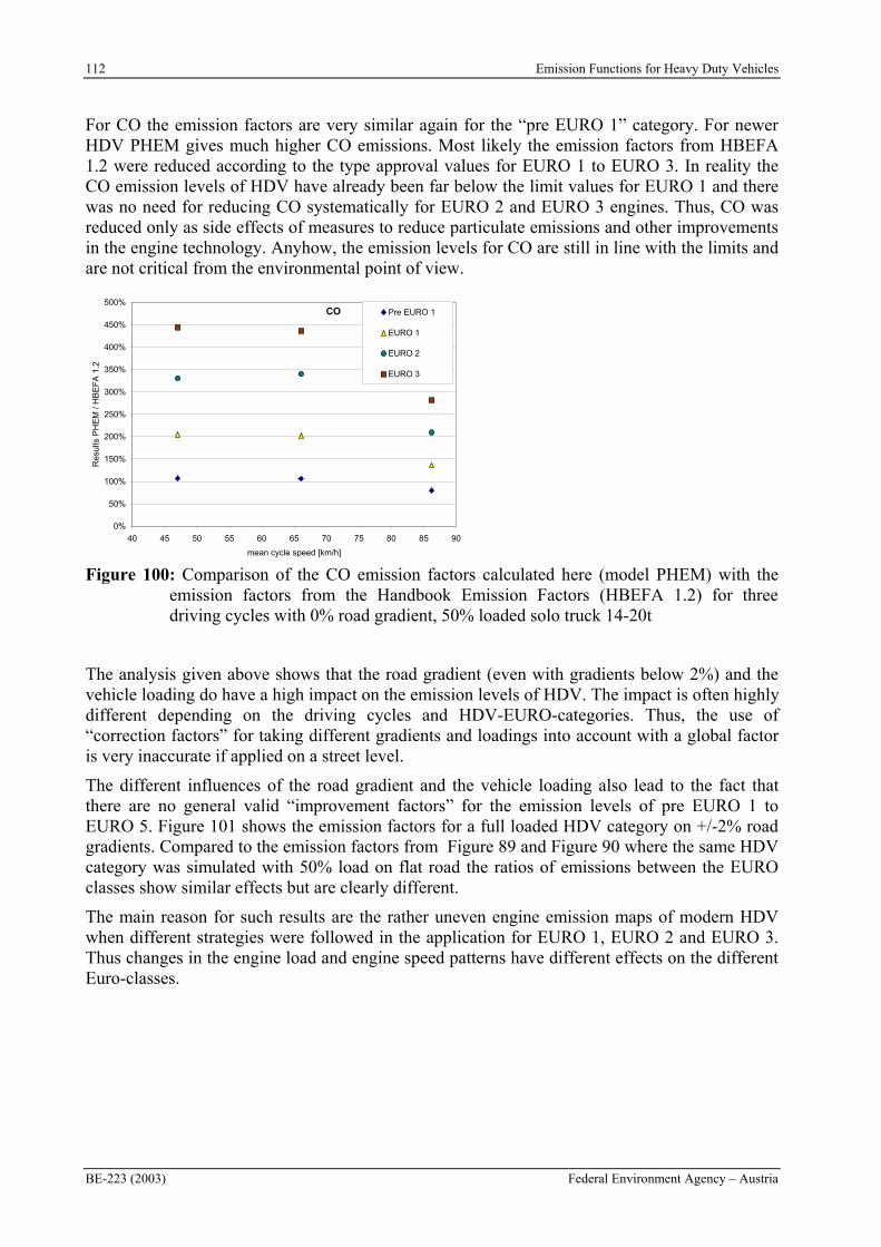
112 Emission Functions for Heavy Duty Vehicles
BE-223 (2003) Federal Environment Agency – Austria
For CO the emission factors are very similar again for the “pre EURO 1” category. For newer HDV PHEM gives much higher CO emissions. Most likely the emission factors from HBEFA 1.2 were reduced according to the type approval values for EURO 1 to EURO 3. In reality the CO emission levels of HDV have already been far below the limit values for EURO 1 and there was no need for reducing CO systematically for EURO 2 and EURO 3 engines. Thus, CO was reduced only as side effects of measures to reduce particulate emissions and other improvements in the engine technology. Anyhow, the emission levels for CO are still in line with the limits and are not critical from the environmental point of view.
0%
50%
100%
150%
200%
250%
300%
350%
400%
450%
500%
40 45 50 55 60 65 70 75 80 85 90
mean cycle speed [km/h]
Res
ults
PH
EM
/ H
BE
FA
1.2
Pre EURO 1
EURO 1
EURO 2
EURO 3
CO
Figure 100: Comparison of the CO emission factors calculated here (model PHEM) with the emission factors from the Handbook Emission Factors (HBEFA 1.2) for three driving cycles with 0% road gradient, 50% loaded solo truck 14-20t
The analysis given above shows that the road gradient (even with gradients below 2%) and the vehicle loading do have a high impact on the emission levels of HDV. The impact is often highly different depending on the driving cycles and HDV-EURO-categories. Thus, the use of “correction factors” for taking different gradients and loadings into account with a global factor is very inaccurate if applied on a street level.
The different influences of the road gradient and the vehicle loading also lead to the fact that there are no general valid “improvement factors” for the emission levels of pre EURO 1 to EURO 5. Figure 101 shows the emission factors for a full loaded HDV category on +/-2% road gradients. Compared to the emission factors from Figure 89 and Figure 90 where the same HDV category was simulated with 50% load on flat road the ratios of emissions between the EURO classes show similar effects but are clearly different.
The main reason for such results are the rather uneven engine emission maps of modern HDV when different strategies were followed in the application for EURO 1, EURO 2 and EURO 3. Thus changes in the engine load and engine speed patterns have different effects on the different Euro-classes.
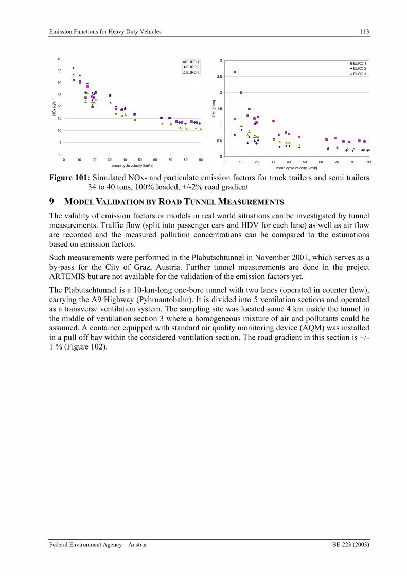
Emission Functions for Heavy Duty Vehicles 113
Federal Environment Agency – Austria BE-223 (2003)
0
5
10
15
20
25
30
35
40
0 10 20 30 40 50 60 70 80 90
mean cycle velocity [km/h]
NO
x [g
/km
]
EURO 1
EURO 2
EURO 3
0
0.5
1
1.5
2
2.5
3
0 10 20 30 40 50 60 70 80 90
mean cycle velocity [km/h]
PM
[g
/km
]
EURO 1
EURO 2
EURO 3
Figure 101: Simulated NOx- and particulate emission factors for truck trailers and semi trailers 34 to 40 tons, 100% loaded, +/-2% road gradient
9 MODEL VALIDATION BY ROAD TUNNEL MEASUREMENTS
The validity of emission factors or models in real world situations can be investigated by tunnel measurements. Traffic flow (split into passenger cars and HDV for each lane) as well as air flow are recorded and the measured pollution concentrations can be compared to the estimations based on emission factors.
Such measurements were performed in the Plabutschtunnel in November 2001, which serves as a by-pass for the City of Graz, Austria. Further tunnel measurements are done in the project ARTEMIS but are not available for the validation of the emission factors yet.
The Plabutschtunnel is a 10-km-long one-bore tunnel with two lanes (operated in counter flow), carrying the A9 Highway (Pyhrnautobahn). It is divided into 5 ventilation sections and operated as a transverse ventilation system. The sampling site was located some 4 km inside the tunnel in the middle of ventilation section 3 where a homogeneous mixture of air and pollutants could be assumed. A container equipped with standard air quality monitoring device (AQM) was installed in a pull off bay within the considered ventilation section. The road gradient in this section is +/- 1 % (Figure 102).
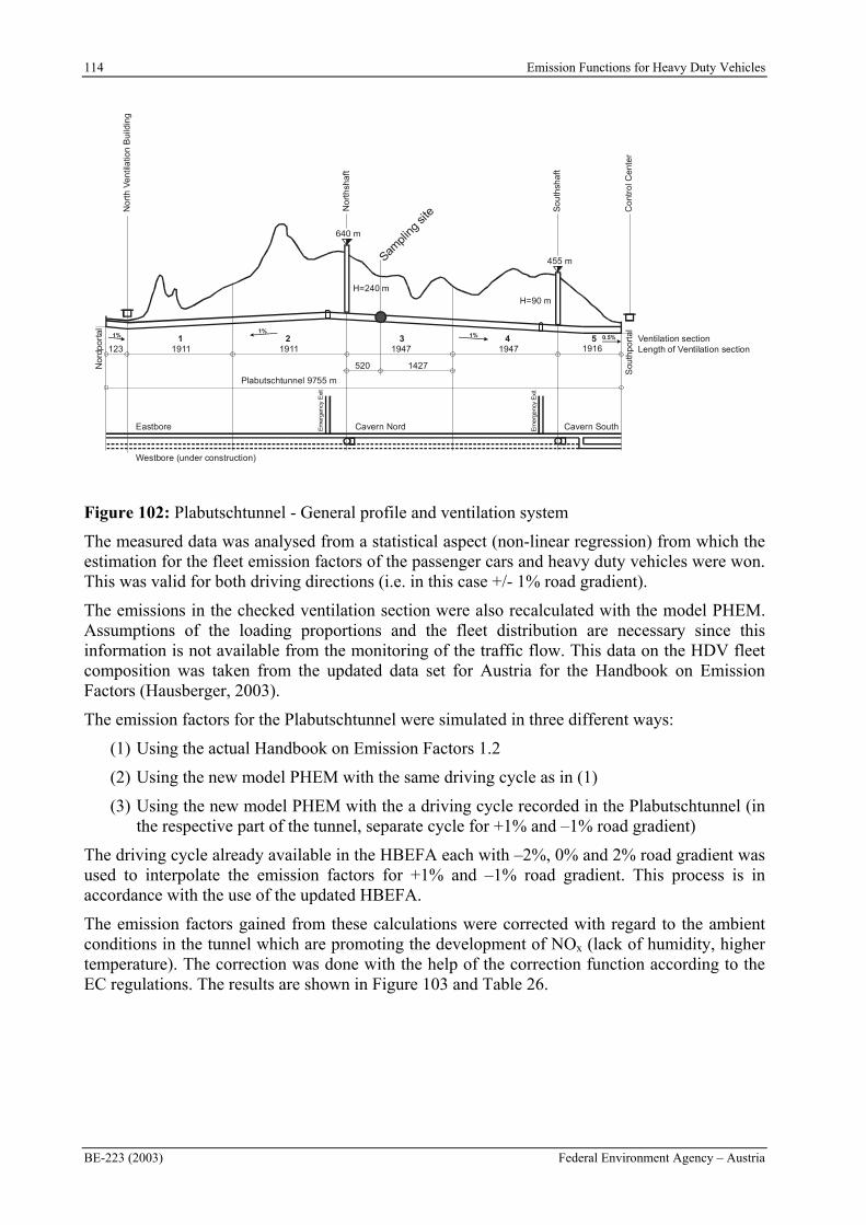
114 Emission Functions for Heavy Duty Vehicles
BE-223 (2003) Federal Environment Agency – Austria
Length of Ventilation sectionVentilation section
123 1911
No
rth
Ve
ntil
atio
n B
uild
ing
No
rdp
ort
al
Sou
thp
ort
al
No
rth
sha
ft
So
uth
sha
ft
Cavern SouthCavern Nord Em
erg
enc
y E
xit
Em
erge
ncy
Exi
t
Co
ntro
l Ce
nte
r
1911
H=240 m
640 m
455 m
H=90 m
1947
520 1427
1947
Plabutschtunnel 9755 m
Sampling
site
Eastbore
Westbore (under construction)
1916543211%
1%1% 0.5%
Figure 102: Plabutschtunnel - General profile and ventilation system
The measured data was analysed from a statistical aspect (non-linear regression) from which the estimation for the fleet emission factors of the passenger cars and heavy duty vehicles were won. This was valid for both driving directions (i.e. in this case +/- 1% road gradient).
The emissions in the checked ventilation section were also recalculated with the model PHEM. Assumptions of the loading proportions and the fleet distribution are necessary since this information is not available from the monitoring of the traffic flow. This data on the HDV fleet composition was taken from the updated data set for Austria for the Handbook on Emission Factors (Hausberger, 2003).
The emission factors for the Plabutschtunnel were simulated in three different ways:
(1) Using the actual Handbook on Emission Factors 1.2
(2) Using the new model PHEM with the same driving cycle as in (1)
(3) Using the new model PHEM with the a driving cycle recorded in the Plabutschtunnel (in the respective part of the tunnel, separate cycle for +1% and –1% road gradient)
The driving cycle already available in the HBEFA each with –2%, 0% and 2% road gradient was used to interpolate the emission factors for +1% and –1% road gradient. This process is in accordance with the use of the updated HBEFA.
The emission factors gained from these calculations were corrected with regard to the ambient conditions in the tunnel which are promoting the development of NOx (lack of humidity, higher temperature). The correction was done with the help of the correction function according to the EC regulations. The results are shown in Figure 103 and Table 26.
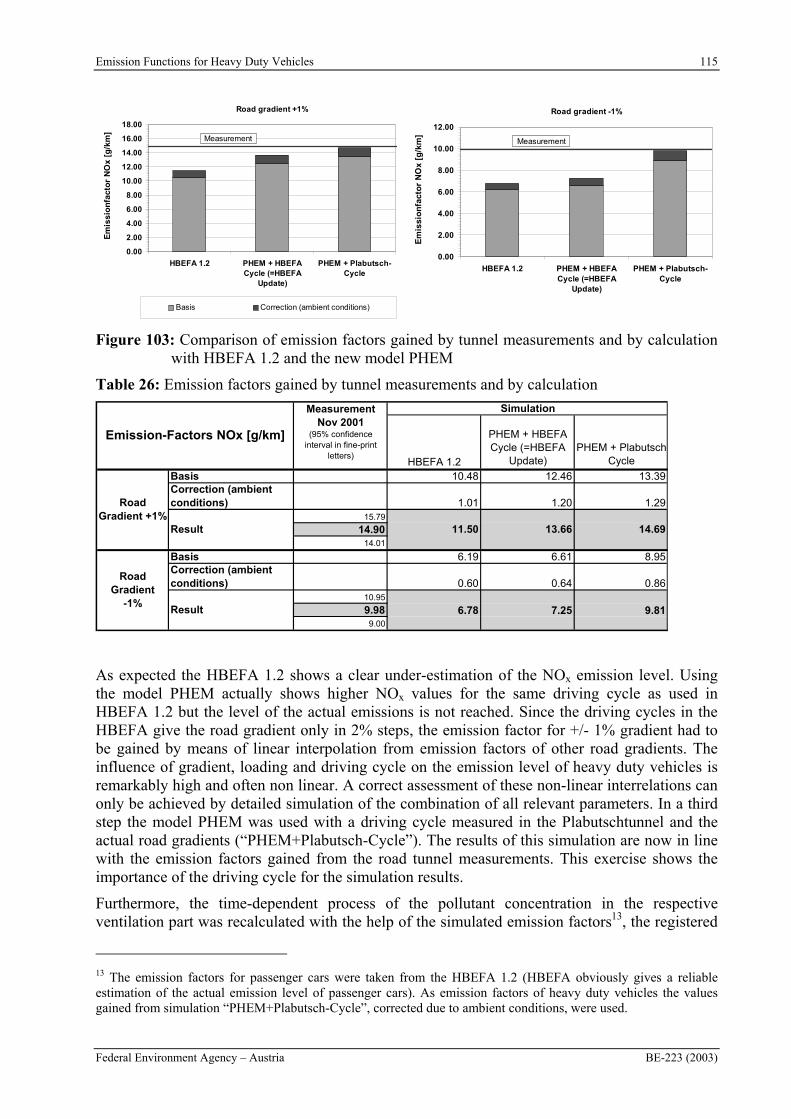
Emission Functions for Heavy Duty Vehicles 115
Federal Environment Agency – Austria BE-223 (2003)
Road gradient +1%
0.00
2.00
4.00
6.00
8.00
10.00
12.00
14.00
16.00
18.00
HBEFA 1.2 PHEM + HBEFACycle (=HBEFA
Update)
PHEM + Plabutsch-Cycle
Em
issi
on
fact
or
NO
x [g
/km
]
Basis Correction (ambient conditions)
Measurement
Road gradient -1%
0.00
2.00
4.00
6.00
8.00
10.00
12.00
HBEFA 1.2 PHEM + HBEFACycle (=HBEFA
Update)
PHEM + Plabutsch-Cycle
Em
issi
on
fact
or
NO
x [g
/km
]
Measurement
Figure 103: Comparison of emission factors gained by tunnel measurements and by calculation with HBEFA 1.2 and the new model PHEM
Table 26: Emission factors gained by tunnel measurements and by calculation
HBEFA 1.2
PHEM + HBEFA Cycle (=HBEFA
Update)PHEM + Plabutsch-
Cycle
Basis 10.48 12.46 13.39Correction (ambient conditions) 1.01 1.20 1.29
15.79
14.9014.01
Basis 6.19 6.61 8.95Correction (ambient conditions) 0.60 0.64 0.86
10.95
9.98 6.78 7.25 9.819.00
Measurement Nov 2001
(95% confidence interval in fine-print
letters)
Simulation
Emission-Factors NOx [g/km]
11.50 13.66 14.69Result
Road Gradient +1%
Road Gradient
-1%Result
As expected the HBEFA 1.2 shows a clear under-estimation of the NOx emission level. Using the model PHEM actually shows higher NOx values for the same driving cycle as used in HBEFA 1.2 but the level of the actual emissions is not reached. Since the driving cycles in the HBEFA give the road gradient only in 2% steps, the emission factor for +/- 1% gradient had to be gained by means of linear interpolation from emission factors of other road gradients. The influence of gradient, loading and driving cycle on the emission level of heavy duty vehicles is remarkably high and often non linear. A correct assessment of these non-linear interrelations can only be achieved by detailed simulation of the combination of all relevant parameters. In a third step the model PHEM was used with a driving cycle measured in the Plabutschtunnel and the actual road gradients (“PHEM+Plabutsch-Cycle”). The results of this simulation are now in line with the emission factors gained from the road tunnel measurements. This exercise shows the importance of the driving cycle for the simulation results.
Furthermore, the time-dependent process of the pollutant concentration in the respective ventilation part was recalculated with the help of the simulated emission factors13, the registered
13 The emission factors for passenger cars were taken from the HBEFA 1.2 (HBEFA obviously gives a reliable estimation of the actual emission level of passenger cars). As emission factors of heavy duty vehicles the values gained from simulation “PHEM+Plabutsch-Cycle”, corrected due to ambient conditions, were used.
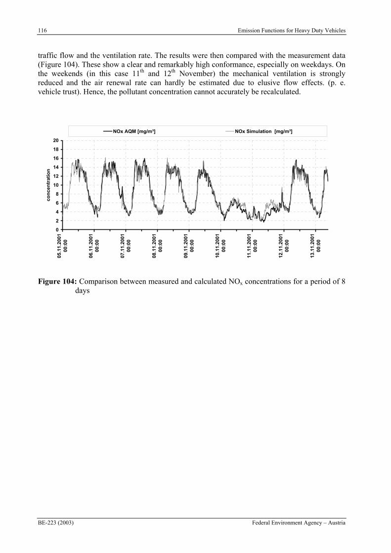
116 Emission Functions for Heavy Duty Vehicles
BE-223 (2003) Federal Environment Agency – Austria
traffic flow and the ventilation rate. The results were then compared with the measurement data (Figure 104). These show a clear and remarkably high conformance, especially on weekdays. On the weekends (in this case 11th and 12th November) the mechanical ventilation is strongly reduced and the air renewal rate can hardly be estimated due to elusive flow effects. (p. e. vehicle trust). Hence, the pollutant concentration cannot accurately be recalculated.
0
2
4
6
8
10
12
14
16
18
20
05.1
1.20
0100
:00
06.1
1.20
0100
:00
07.1
1.20
0100
:00
08.1
1.20
0100
:00
09.1
1.20
0100
:00
10.1
1.20
0100
:00
11.1
1.20
0100
:00
12.1
1.20
0100
:00
13.1
1.20
0100
:00
con
cen
trat
ion
NOx AQM [mg/m³] NOx Simulation [mg/m³]
Figure 104: Comparison between measured and calculated NOx concentrations for a period of 8 days
Emission Functions for Heavy Duty Vehicles 117
Federal Environment Agency – Austria BE-223 (2003)
10 SUMMARY
The work performed within the project gave a lot of new insight into the emission behaviour of modern HDV and the technical background. The measurement programme elaborated and the method developed for the simulation of HDV emission factors proved to be capable of handling these new technologies. Future measurement programmes may try to include measurements also at map points with about zero torque and engine speeds above idling.
Emission measurements for 124 HDV-engines and for 7 HDV are gained from the measurement programme and the data collection. 13 of the engine tests include extensive steady state tests and different transient test cycles. For the other engines only steady state measurements have been performed. 61 of the engines were finally included into the model. This confirms the methodology selected for the HDV vehicle emission model which is based on steady state engine emission maps. The collection of already existing data and the actual measurement programme clearly benefits from the cooperation with COST 346, ARTEMIS-WP 400 and several national activities. Without this cooperation the number of available measurements would have been much smaller (45 engines, 30 of them pre Euro 1).
The model PHEM developed for simulating HDV emission factors reaches a very high accuracy by using a detailed simulation of the effective engine power demand and the engine speed. The method of interpolating emissions from the engine maps is well tuned with the design of the standardised engine emission map format. The standardised format also allows the averaging of emission maps gained from engines with different sizes. This method improves the sample size per vehicle category in the Handbook on average by a factor of ten, what makes the emission factors much more reliable. A main tool for reaching high accuracies is the method developed for the transient correction. This method transforms the emission levels from the engine map, which is measured under steady state conditions, on the emission levels which have to be expected in transient engine loads.
The model PHEM also proved to be capable of handling the requests of the Handbook on Emission Factors on the simulation of emission factors for traffic situations of which no measured driving cycles were available. A validation of the new emission factors for HDV was performed using air quality measurements in a road tunnel. The new model actually matches the results of the tunnel measurements very well while older emission factors always showed clear underestimations.
Results show that the emission levels did not decrease since the introduction of EURO 1 limits in real world driving conditions in the same order of magnitude as the emission limits for the type approval were reduced. The main reasons are found in the more sophisticated technologies for engine control and fuel injection which allow different specific optimisations for different regions of the engine map. The steady state tests at the type approval can not ensure low emission levels for real world driving conditions.
These new results clearly diverge from the emission factors for Euro 2 and Euro 3 HDV used in the Handbook Emission Factors (HBEFA 1.2) until now but are in line with the analysis of air quality measurements on road sites.
In total for more than 30.000 combinations of vehicle categories, EURO-categories, driving cycles, vehicle loadings and road gradients emission factors were simulated with the model PHEM. The analysis of the results is in line with the assessment of the engine tests. Due to the different strategies for the application work at the engines for EURO 1, EURO 2 and EURO 3 the behaviour of the HDV under different vehicle loads, driving cycles and road gradient is very different for the different EURO classes. Thus, simplified methods for assessing the emissions of HDV have to be used carefully.

Emission Functions for Heavy Duty Vehicles 119
Federal Environment Agency – Austria BE-223 (2003)
11 LITERATURE
Evéquoz R.: Emissionsfaktoren von schweren Motorwagen in der Schweiz, Schlußbericht; Bundesamt für Umwelt, Wald und Landschaft (BUWAL); Umwelt-Materialien Nr. 38; Luft: Bern 1995
Hammarström, U. and Karlsson, B. VETO – a computer programme for calculation of transport costs as a function of road standard. VTI Meddelande 501. Swedish Road and Traffic Research Institute. Linköping. 1987.
Hassel D., Jost P. et al.: Abgas-Emissionsfaktoren von Nutzfahrzeugen in der Bundesrepublik Deutschland für das Bezugsjahr 1990; Luftreinhaltung UFO PLAN-Nr. 104 05 151/02; TÜV-Rheinland Sicherheit und Umweltschutz GmbH im Auftrag des Umweltbundesamtes; Berlin 1995
Hausberger S.: Planung und Koordination zur „Aktualisierung der Emissionsfaktoren für Schwere Nutzfahrzeuge“; Institut für Verbrennungskraftmaschinen und Thermodynamik der TU-Graz; 1998
Hausberger S. et.al.: Description of the Measurement Programme for HDV, Deliverable 10 within the EU-5th Framework Project ARTEMIS, February 2001
Hausberger S. et.al.: Results from the Review and Model Description, Deliverable 11 within the EU-5th Framework Project ARTEMIS, March 2001
Huncho W.H..: Aerodynamic of Road vehicles. Fourth edition p. 415-488; 1998
Keller M., Hausberger S. et.al.:: Handbuch Emissionsfaktoren für den Straßenverkehr in Österreich (Guide on Emission Factors for the Street Traffic in Austria); im Auftrag von Bundesministerium für Umwelt, Jugend und Familie und Umweltbundesamt Österreich; Wien 1998
Lastauto Omnibus Katalog: years 1995 to 2001.
Mitschke M.: Dynamik der Kraftfahrzeuge; 2. Auflage; Springer Verlag Berlin, 1982
Nakamura S. et.al: LES Simulation of Aerodynamic Drag for Heavy Duty Trailer Trucks; proceedings of the ASME Fluid Division Summer Meeting; Montreal, Quebec; July 14 to 18 2002
Riemersma en P I.J.. Hendriksen, Praktijkemissies van een HD motor, december 1999, TNO-rapport 99.OR.VM.060.1/IJR, Delft (only available in Dutch language)
Rijkeboear R.C. et.al.: Final Report In-use Compliance programme; Trucks 1996 – 1997; TNO report 99.OR.VM.040.1/RR; TNO Automotive; Nov. 1998
Roumégoux J-P.: The SIMULCO software: description of modelling and examples of application; Development and Application of Computer Techniques to Environmental Studies, Envirosoft 96; Como, sept. 1996
Saltzman E.J. et.al.: A Reassessment of Heavy-Duty Truck Aerodynamic Design Features and Priorities; NASA/TP 1999-206574; June 1999
Steven H.: Auswertung des Fahrverhaltens von schweren Motorwagen; FIGE GmbH; BUWAL; 1995
Tieber J.: Eine globale Methode zur Berechnung des Emissionsverhaltens von Nutzfahrzeugen „A holistic method for calculating HDV emissions“ , Dissertation, TU-Graz, 1997.
120 Emission Functions for Heavy Duty Vehicles
BE-223 (2003) Federal Environment Agency – Austria
Van de Weijer C.J.T., Heavy-Duty Emission Factors - Development of representative driving cycles and prediction of emissions in real-life, Technical University Graz, October 1997, Delft
Van de Venne J.W.C.M., R.C. Rijkeboer, Rekenmodel voor emissie en brandstofverbruik van bedrijfswagens en het schatten van ontwikkelingtendensen voor de modelparameters, TNO report 95.OR.VM.072.1/JvdV, februari 1996, Delft (only available in Dutch language)
Van de Venne J.W.C.M., R.T.M. Smokers, TNO-ADVANCE - A Modular Powertrain Simulation and Design Tool, TNO Paper VM 0002, 2000, Delft
Verkiel M., Ontwikkeling van het voertuigsimulatieprogramma ADVANCE, Technical University Delft, MT OEMO 96/09, May 1997, Delft (only available in Dutch language)
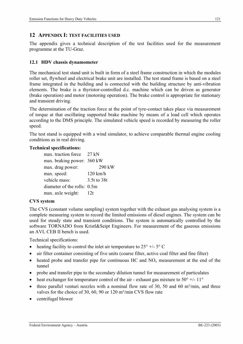
Emission Functions for Heavy Duty Vehicles 121
Federal Environment Agency – Austria BE-223 (2003)
12 APPENDIX I: TEST FACILITIES USED
The appendix gives a technical description of the test facilities used for the measurement programme at the TU-Graz.
12.1 HDV chassis dynamometer
The mechanical test stand unit is built in form of a steel frame construction in which the modules roller set, flywheel and electrical brake unit are installed. The test stand frame is based on a steel frame integrated in the building and is connected with the building structure by anti-vibration elements. The brake is a thyristor-controlled d.c. machine which can be driven as generator (brake operation) and motor (motoring operation). The brake control is appropriate for stationary and transient driving.
The determination of the traction force at the point of tyre-contact takes place via measurement of torque at that oscillating supported brake machine by means of a load cell which operates according to the DMS principle. The simulated vehicle speed is recorded by measuring the roller speed.
The test stand is equipped with a wind simulator, to achieve comparable thermal engine cooling conditions as in real driving.
Technical specifications: max. traction force 27 kN max. braking power: 360 kW max. drag power: 290 kW max. speed: 120 km/h vehicle mass: 3.5t to 38t diameter of the rolls: 0.5m max. axle weight: 12t
CVS system
The CVS (constant volume sampling) system together with the exhaust gas analysing system is a complete measuring system to record the limited emissions of diesel engines. The system can be used for steady state and transient conditions. The system is automatically controlled by the software TORNADO from Kristl&Seipt Engineers. For measurement of the gaseous emissions an AVL CEB II bench is used.
Technical specifications:
heating facility to control the inlet air temperature to 25° +/- 5° C
air filter container consisting of five units (coarse filter, active coal filter and fine filter)
heated probe and transfer pipe for continuous HC and NOx measurement at the end of the tunnel
probe and transfer pipe to the secondary dilution tunnel for measurement of particulates
heat exchanger for temperature control of the air - exhaust gas mixture to 50° +/- 11°
three parallel venturi nozzles with a nominal flow rate of 30, 50 and 60 m³/min, and three valves for the choice of 30, 60, 90 or 120 m³/min CVS flow rate
centrifugal blower
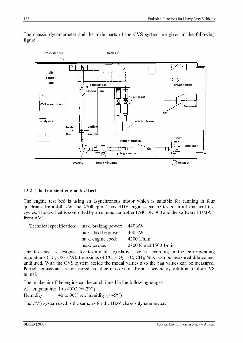
122 Emission Functions for Heavy Duty Vehicles
BE-223 (2003) Federal Environment Agency – Austria
The chassis dynamometer and the main parts of the CVS system are given in the following figure.
CVS -Steuerung
Abgasanalyse
Rollen -
Beobachtungs-
raum
Beheizte Leitung
(HC, NOx)
Partikel
Probe
Abgas
Fahrtwindsimulator
Filterkästen Frischluft
Laval - Düsen
Abgaskamin
Probenentnahme Beutel
Zyklon
Ventilator
Rollensatz
elektrische Bremse
Verdünnungs-
tunnel
Wärmetauscher
Fahrerbildschirm
CVS -Steuerung
Abgasanalyse
Rollen -
Beobachtungs-
raum
Beheizte Leitung
(HC, NOx)
Partikel
Probe
Abgas
Fahrtwindsimulator
Filterkästen Frischluft
Laval - Düsen
Abgaskamin
Probenentnahme Beutel
Zyklon
Ventilator
Rollensatz
elektrische Bremse
Verdünnungs-
tunnel
Wärmetauscher
Fahrerbildschirm
CVS –control unit
analyzers
roller
control
unit
heated
line
particle
sample
exhaust gas
fan
fresh air filter fresh air
venturi nozzles
exhaust
bag sample
cyclone
ventilator
roller set
electric brake
dilution tunnel
heat exchanger
driver screen
12.2 The transient engine test bed
The engine test bed is using an asynchronous motor which is suitable for running in four quadrants from 440 kW and 4200 rpm. Thus HDV engines can be tested in all transient test cycles. The test bed is controlled by an engine controller EMCON 300 and the software PUMA 5 from AVL.
Technical specification: max. braking power: 440 kW max. throttle power: 400 kW max. engine sped: 4200 1/min max. torque: 2800 Nm at 1500 1/min
The test bed is designed for testing all legislative cycles according to the corresponding regulations (EC, US-EPA). Emissions of CO, CO2, HC, CH4, NOx can be measured diluted and undiluted. With the CVS system beside the modal values also the bag values can be measured. Particle emissions are measured as filter mass value from a secondary dilution of the CVS tunnel.
The intake air of the engine can be conditioned in the following ranges: Air temperature: 1 to 40°C (+/-2°C) Humidity: 40 to 90% rel. humidity (+/-5%)
The CVS system used is the same as for the HDV chassis dynamometer.
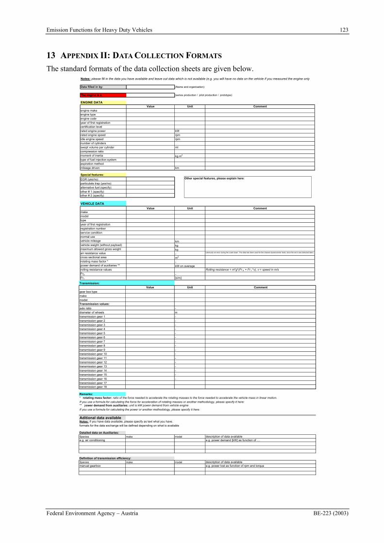
Emission Functions for Heavy Duty Vehicles 123
Federal Environment Agency – Austria BE-223 (2003)
13 APPENDIX II: DATA COLLECTION FORMATS
The standard formats of the data collection sheets are given below. Notes: please fill in the data you have available and leave out data which is not available (e.g. you will have no data on the vehicle if you measured the engine only
Data filled in by: (Name and organisation)
The engine is a (series production / pilot production / prototype)
ENGINE DATAValue Unit Comment
engine makeengine type
engine code
year of first registration
certification level
rated engine power kW
rated engine speed rpm
idle engine speed rpm
number of cylinders
swept volume per cylinder ml
compression ratio
moment of inertia kg.m2
type of fuel injection system
aspiration method
mileage driven km
Special features:
EGR (yes/no)
particulate trap (yes/no)
alternative fuel (specify)
other # 1 (specify)other # 2 (specify)
VEHICLE DATA
Value Unit Commentmake
model
type
year of first registration
registration number
service condition
normal use
vehicle mileage kmvehicle weight (without payload) kgmaximum allowed gross weight kgair resistance value - (obviously an error during the coast down. The data has been used for the chassis dynamometer tests, since the error was detected later)
cross sectional area m2
rotating mass factor * -power demand of auxiliaries ** kW on averagerolling resistance values Rolling resistance = m*g*(Fr 0 + Fr 1 *v), v = speed in m/sFr0 -Fr1 [s/m]
Other special features, please explain here:
Transmission:
Value Unit Comment
gear box type
make
modelTransmission values:
axle ratio -
diameter of wheels m
transmission gear 1 -
transmission gear 2 -
transmission gear 3 -
transmission gear 4 -
transmission gear 5 -
transmission gear 6 -
transmission gear 7 -
transmission gear 8 -
transmission gear 9 -
transmission gear 10 -
transmission gear 11 -
transmission gear 12 -
transmission gear 13 -
transmission gear 14 -
transmission gear 15 -
transmission gear 16 -
transmission gear 17transmission gear 18
Remarks:* rotating mass factor: ratio of the force needed to accelerate the rotating masses to the force needed to accelerate the vehicle mass in linear motion.If you use a formula for calculating the force for acceleration of rotating masses or another methodology, please specify it here:** power demand from auxiliaries: unit is kW power demand from vehicle engineIf you use a formula for calculating the power or another methodology, please specify it here:
Aditional data availableNotes: if you have data available, please specify as text what you have. formats for the data exchange will be defined depending on what is available
Datailed data on Auxiliaries:Species make model description of data availablee.g. air conditioning e.g. power demand [kW] as function of ....
Definition of transmission efficiency:Species make model description of data availablemanual gearbox e.g. power lost as function of rpm and torque

124 Emission Functions for Heavy Duty Vehicles
BE-223 (2003) Federal Environment Agency – Austria
Full load curve:
Comment: number of values (lines) to be filled in is free, data given here is an example with 24 values
Fuel used: (standard diesel, Biodiesel, CNG,....)
Full load curve:Column A Column BNominal engine speed [rpm] Power [kW]
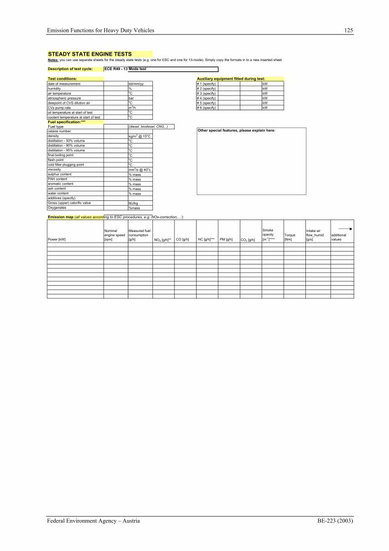
Emission Functions for Heavy Duty Vehicles 125
Federal Environment Agency – Austria BE-223 (2003)
STEADY STATE ENGINE TESTSNotes: you can use separate sheets for the steady state tests (e.g. one for ESC and one for 13-mode). Simply copy the formats in to a new inserted sheet
Description of test cycle: ECE R49 - 13 Mode test
Test conditions: Auxiliary equipment fitted during test:date of measurement dd/mm/yy # 1 (specify) kWhumidity % # 2 (specify) kWair temperature oC # 3 (specify) kWatmospheric pressure bar # 4 (specify) kWdewpoint of CVS dilution air oC # 5 (specify) kWCVs pump rate m3/h # 6 (specify) kWoil temperature at start of test oC
coolant temperature at start of test oC
Fuel specification:***Fuel type (diesel, biodiesel, CNG,..)cetane numberdensity kg/m3 @ 15oCdistillation - 50% volume oCdistillation - 90% volume oCdistillation - 95% volume oCfinal boiling point oCflash point oCcold filter plugging point oCviscosity mm2/s @ 40ocsulphur content % massPAH content % massaromatic content % massash content % masswater content % massadditives (specify)Gross (upper) calorific value MJ/kgOxygenates %mass
Emission map (all values according to ESC procedures, e.g. NOx-correction,... ):
Power [kW]
Nominal engine speed [rpm]
Measured fuel consumption [g/h] NOX [g/h]** CO [g/h] HC [g/h]*** PM [g/h] CO2 [g/h]
Smoke opacity
[m-1]****Torque [Nm]
Intake air flow_humid [g/s]
additional values
Other special features, please explain here:
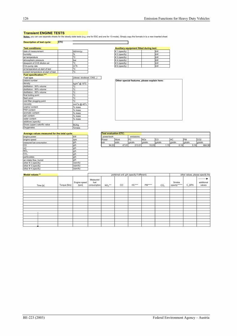
126 Emission Functions for Heavy Duty Vehicles
BE-223 (2003) Federal Environment Agency – Austria
Transient ENGINE TESTSNotes: you can use separate sheets for the steady state tests (e.g. one for ESC and one for 13-mode). Simply copy the formats in to a new inserted sheet
Description of test cycle: ETC
Test conditions: Auxiliary equipment fitted during test:date of measurement dd/mm/yy # 1 (specify) kWhumidity % # 2 (specify) kWair temperature oC # 3 (specify) kWatmospheric pressure bar # 4 (specify) kWdewpoint of CVS dilution air oC # 5 (specify) kWCVs pump rate m3/h # 6 (specify) kWoil temperature at start of test oC
coolant temperature at start of test oC
Fuel specification:***Fuel type (diesel, biodiesel, CNG,..)cetane numberdensity kg/m3 @ 15oCdistillation - 50% volume oCdistillation - 90% volume oCdistillation - 95% volume oCfinal boiling point oCflash point oCcold filter plugging point oCviscosity mm2/s @ 40ocsulphur content % massPAH content % massaromatic content % massash content % masswater content % massadditives (specify)Gross (upper) calorific value MJ/kgOxygenates %mass
Average values measured for the total cycle: Test evaluation ETC:engine power kW power/work emissions
engine speed rpm Power Work FC NOx CO HC PM CO2measured fuel consumption g/h kW kWh g/kWh g/kWh g/kWh g/kWh g/kWh g/kWhCO g/h 94.03 47.01 213.01 10.03 1.15 0.18 0.16 664.98
HC g/hNOX g/hCO2 g/hparticulates g/h
air intake flow_humid g/hother # 2 (specify) (specify)
other # 3 (specify) (specify)
other # 4 (specify) (specify)
Modal values:** preferred unit: g/h (specify if different) other values, please specify the
Time [s] Torque [Nm]Engine speed
[rpm]
Measured fuel
consumption NOX*** CO HC**** PM***** CO2
Smoke opacity****** C_DPA
additional values
Other special features, please explain here:
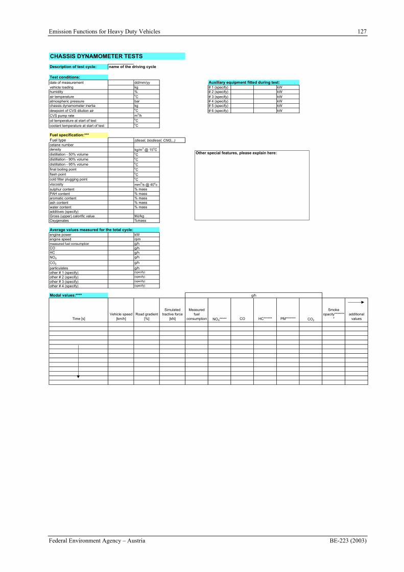
Emission Functions for Heavy Duty Vehicles 127
Federal Environment Agency – Austria BE-223 (2003)
CHASSIS DYNAMOMETER TESTS
Description of test cycle: name of the driving cycle
Test conditions:date of measurement dd/mm/yy Auxiliary equipment fitted during test:vehicle loading kg # 1 (specify) kWhumidity % # 2 (specify) kWair temperature oC # 3 (specify) kWatmospheric pressure bar # 4 (specify) kWchassis dynamometer inertia kg # 5 (specify) kW
dewpoint of CVS dilution air oC # 6 (specify) kWCVS pump rate m3/h
oil temperature at start of test oC
coolant temperature at start of test oC
Fuel specification:***Fuel type (diesel, biodiesel, CNG,..)cetane numberdensity kg/m3 @ 15oCdistillation - 50% volume oCdistillation - 90% volume oCdistillation - 95% volume oCfinal boiling point oCflash point oCcold filter plugging point oCviscosity mm2/s @ 40ocsulphur content % massPAH content % massaromatic content % massash content % masswater content % massadditives (specify)Gross (upper) calorific value MJ/kgOxygenates %mass
Average values measured for the total cycle:engine power kWengine speed rpmmeasured fuel consumption g/hCO g/hHC g/hNOX g/h
CO2 g/h
particulates g/hother # 1 (specify) (specify)
other # 2 (specify) (specify)
other # 3 (specify) (specify)
other # 4 (specify) (specify)
Modal values:****
Time [s]Vehicle speed
[km/h]Road gradient
[%]
Simulated tractive force
[kN]
Measured fuel
consumption NOX***** CO HC****** PM******* CO2
Smoke opacity*******
*additional
values
g/h
Other special features, please explain here:
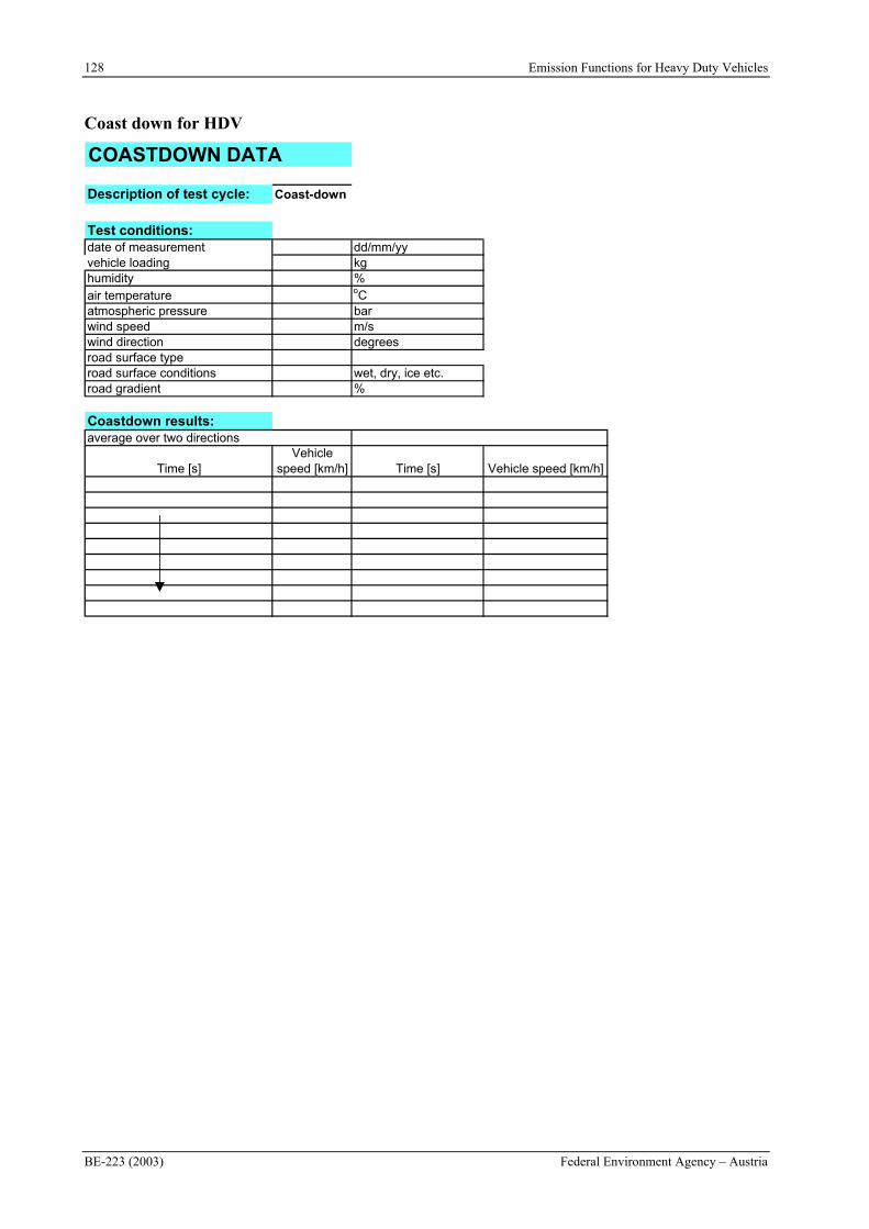
128 Emission Functions for Heavy Duty Vehicles
BE-223 (2003) Federal Environment Agency – Austria
Coast down for HDV
COASTDOWN DATA
Description of test cycle: Coast-down
Test conditions:date of measurement dd/mm/yyvehicle loading kghumidity %air temperature oCatmospheric pressure barwind speed m/swind direction degreesroad surface typeroad surface conditions wet, dry, ice etc.road gradient %
Coastdown results:average over two directions
Time [s]Vehicle
speed [km/h] Time [s] Vehicle speed [km/h]