ELECTROSTATIC INTERACTION BETWEEN TWO CONDUCTING SPHERES

Kiril Kolikov, Dragia Ivanov, Georgi Krastev †, Yordan Epitropov*, Stefan Bozhkov

Plovdiv University ‘P. Hilendarski’ – 24 Tzar Asen Str., Plovdiv, Bulgaria

Abstract

In the paper we consider the problem of the electrostatic interaction between two charged

conducting spheres with arbitrary electrical charges and radiuses. Using the image charges method

we determine exact analytical formulas for the force F and for the potential energy W of the

interaction between these two spheres as well as for the potential V of the electromagnetic field in

an arbitrary point created by them. Our formulas lead to Coulomb’s law for point charges.

We theoretically prove the experimentally shown fact that two spheres with the same type

(positive or negative) of charges can also attract each other.

Key words: conducting sphere; Coulomb’s law; image charges method; electric interaction;

potential energy of electrostatic interaction; potential of electrostatic field.

1. Introduction

The problem for determining the electrostatic force of interaction between two charged

conducting spheres with arbitrary radiuses and charges is firstly investigated in a complex way by

Poisson. Later, Sir Thompson (Lord Kelvin) introduces his image charges theory thus significantly

simplifying the investigation. This theory is based on the function of influence of a point source in

the three dimensional case for the first boundary problem for the Poisson’s equation. This method

eliminates the need to solve the Laplace’s equation in order to determine the distribution of the

image charges whose electric fields have to meet certain boundary conditions.

This problem is later on considered by Maxwell ([1], Chapter 1). He discovers that the

electrostatic force between the two spheres with charges 1

Q and 2Q is different from the electrostatic

force between the point charges 1

Q and 2Q located at the centres of the spheres respectively, which

is derived by Coulomb’s law. According to Maxwell this deviation is caused by the redistribution of

the charges as a result of the mutual electrostatic influence between the spheres.

* Corresponding author.

E-mail address: epitropov@uni-plovdiv.bg (Y. Epitropov)

Having in mind the redistribution of the charges, Maxwell suggest a general method for

determining the force of interaction between two spheres with arbitrary charges and radiuses using

zonal harmonics with complex mathematical apparatus ([1], Chapters 11-13). Many scientists after

him find other principle solutions to the problem. In different special cases they derive exact

formulas or give approximate formulas which are good enough for the solution of some theoretical

or practical problems.

The electrostatic force F and the potential energy W of the electrostatic interaction between two

conducting spheres, as well as the potential V of the created electrostatic field can be determined

analytically using the method of integration [2], the method of electrical inducted coefficients [3] or

the image charges method [1, 4, 5].

The image charges method has two main directions.

In the first direction (for example [6], [7], [8], [9]) it is considered how the outer electric field

firstly induces dipole in the centre of each sphere. After that these two dipoles induce iteratively a

sequence of image dipoles in the spheres.

In the second direction the electric field created by the electric charges in the two conducting

spheres is considered. Each of the two initial charges induces image charges in the other sphere;

these charges themselves induce respectively new image charges in the given spheres and so on. In

order to construct the images transformation by inversion [1, 4, 5] is used. Analysing this process,

the distribution of the charge in each sphere can be determined. This method yields very complex

analytical form of the results. Thus there are many, but approximate or partial results.

Smythe uses the image charges method in order to determine the electrostatic force between two

spheres, which are not intersecting, with arbitrary charges and radiuses [4, Chapter 5]. Moreover, he

considers the special case when one of the spheres is grounded using hyperbolical functions. He also

calculates the first few terms in a sum describing the force as a function of the capacities of the

spheres.

Jackson considers a number of special cases and the application of Green’s functions, Laplace’s

equation and Fourier’s series with regards to this problem [10, Chapter 2]. He does not give a

solution to the problem in the general case but using the image charges method he describes the path

for discovering the solution of the problem for two spheres, which are not intersecting, with different

radiuses and charges by pointing out how the induced charges and their locations can be determined

iteratively.

Soules analyses Coulomb’s trials and conducts precise experiments having in mind the induction

effects [11]. He uses the image charges method to develop a computer program in order to determine

numerically the force of interaction. Based on the analysis of the numerical values (and not

theoretically) Soules also suggests an approximated formula for the electrostatic force.

A number of authors using the image charges method derive approximate formulas for the force

of interaction between two charged conducting spheres in the special case when they are with equal

radiuses and charges [12, 13]. Such formula is found by Slisko and Brito-Orta and using a computer

program they compare the values calculated using different approximations, thus showing that

Larson – Goss’ and Soules’ formulas are wrong [13]. However, they also conclude that when the

distance between the spheres is rather small compared to their radiuses their ‘analytical approaches

turn out to be very impractical’ ([13], p. 353).

In the current paper we further develop the image charges method, also considered by us in [14].

We derive in the most basic form exact analytical formulas for F , W and V created by two charged

conducting spheres, with arbitrary charges and radiuses, which are not grounded. Moreover, we use

an easily applicable algebraic method which overcomes all of the above mentioned disadvantages.

Our formulas lead to Coulomb’s law when 021== rr . Furthermore, we determine the deviation

between the values of F , W and V for charged conducting spheres and their corresponding values

0F ,

0W and

0V for point charges. We also theoretically show that two spheres with the same type

(positive or negative) of charges can also attract each other – a fact which is experimentally shown.

2. Electrostatic interaction between two charged conducting spheres

Let 1S and

2S are two charged conducting spheres, which are not grounded, with charges

respectively 1

Q , 2Q and radiuses

1r ,

2r and R is the distance between their centres

1O ,

2O in the

inertial system J (Fig. 1). As the charges 1

Q and 2Q are equally spread on the surfaces of

1S and

2S , we assume that before the interaction of the spheres they are concentrated respectively in the

centres 1

O and 2O .

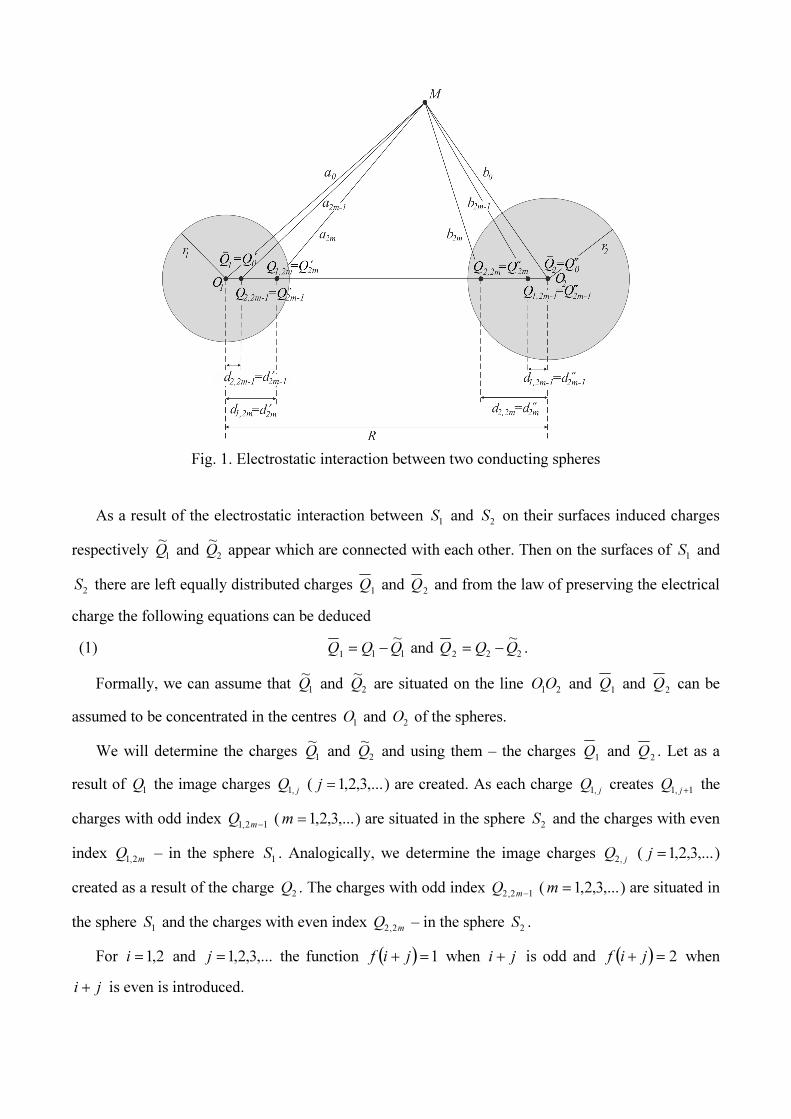
Fig. 1. Electrostatic interaction between two conducting spheres

As a result of the electrostatic interaction between 1S and

2S on their surfaces induced charges

respectively 1

~

Q and 2

~

Q appear which are connected with each other. Then on the surfaces of 1S and

2S there are left equally distributed charges

1Q and

2Q and from the law of preserving the electrical

charge the following equations can be deduced

(1) 111

~

QQQ −= and 222

~

QQQ −= .

Formally, we can assume that 1

~

Q and 2

~

Q are situated on the line 21OO and

1Q and

2Q can be

assumed to be concentrated in the centres 1

O and 2O of the spheres.

We will determine the charges 1

~

Q and 2

~

Q and using them – the charges 1Q and

2Q . Let as a

result of 1

Q the image charges j

Q,1

( ,...3,2,1=j ) are created. As each charge j

Q,1

creates 1,1 +j

Q the

charges with odd index 12,1 −m

Q ( ,...3,2,1=m ) are situated in the sphere 2

S and the charges with even

index mQ

2,1 – in the sphere

1S . Analogically, we determine the image charges

jQ

,2 ( ,...3,2,1=j )

created as a result of the charge 2Q . The charges with odd index

12,2 −mQ ( ,...3,2,1=m ) are situated in

the sphere 1S and the charges with even index

mQ

2,2 – in the sphere

2S .

For 2,1=i and ,...3,2,1=j the function ( ) 1=+ jif when ji + is odd and ( ) 2=+ jif when

ji + is even is introduced.

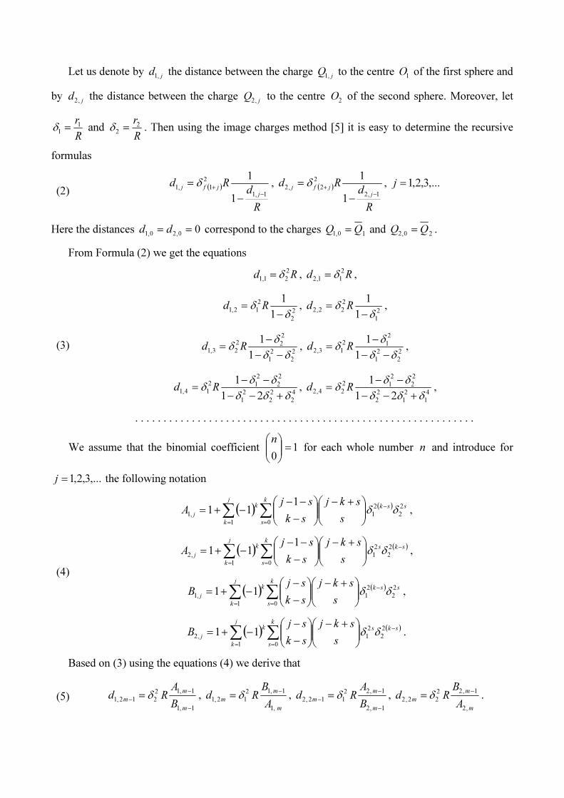
Let us denote by j

d,1

the distance between the charge j

Q,1

to the centre 1

O of the first sphere and

by j

d,2

the distance between the charge jQ

,2 to the centre

2O of the second sphere. Moreover, let

R

r1

1=δ and

R

r2

2=δ . Then using the image charges method [5] it is easy to determine the recursive

formulas

(2) ( )

R

dRd

jjfj

1,1

2

1,1

1

1

−

+

−

= δ , ( )

R

dRd

jjfj

1,2

2

2,2

1

1

−

+

−

= δ , ,...3,2,1=j

Here the distances 00,20,1== dd correspond to the charges

10,1QQ = and

20,2QQ = .

From Formula (2) we get the equations

(3)

Rd2

21,1δ= , Rd

2

11,2δ= ,

2

2

2

12,11

1

δδ

−

= Rd , 2

1

2

22,21

1

δδ

−

= Rd ,

2

2

2

1

2

22

23,11

1

δδ

δδ

−−

−= Rd ,

2

2

2

1

2

12

13,21

1

δδ

δδ

−−

−

= Rd ,

4

2

2

2

2

1

2

2

2

12

14,121

1

δδδ

δδδ

+−−

−−= Rd ,

4

1

2

1

2

2

2

2

2

12

24,221

1

δδδ

δδδ

+−−

−−= Rd ,

. . . . . . . . . . . . . . . . . . . . . . . . . . . . . . . . . . . . . . . . . . . . . . . . . . . . . . . . . . . .

We assume that the binomial coefficient 10

=

n for each whole number n and introduce for

,...3,2,1=j the following notation

(4)

( ) ( )∑ ∑= =

−

+−

−

−−−+=

j

k

k

s

sskk

js

skj

sk

sjA

1 0

2

2

2

1,1

111 δδ ,

( ) ( )∑ ∑= =

−

+−

−

−−−+=

j

k

k

s

sksk

js

skj

sk

sjA

1 0

2

2

2

1,2

111 δδ ,

( ) ( )∑ ∑= =

−

+−

−

−−+=

j

k

k

s

sskk

js

skj

sk

sjB

1 0

2

2

2

1,111 δδ ,

( ) ( )∑ ∑= =

−

+−

−

−−+=

j

k

k

s

sksk

js

skj

sk

sjB

1 0

2

2

2

1,211 δδ .

Based on (3) using the equations (4) we derive that

(5) 1,1

1,12

212,1

−

−

−

=

m

m

m

B

ARd δ ,

m

m

m

A

BRd

,1

1,12

12,1

−

= δ , 1,2

1,22

112,2

−

−

−

=

m

m

m

B

ARd δ ,

m

m

m

A

BRd

,2

1,22

22,2

−

= δ .

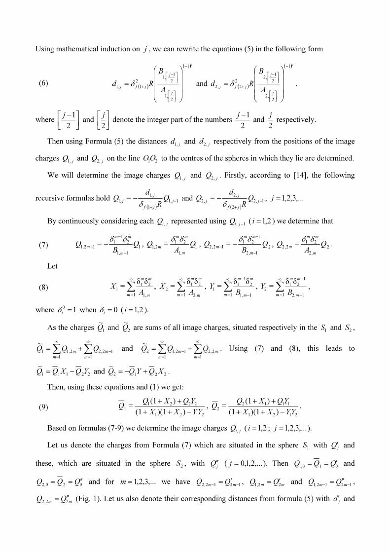
Using mathematical induction on j , we can rewrite the equations (5) in the following form

where

−

2

1j and

2

j denote the integer part of the numbers

2

1−j and

2

j respectively.

Then using Formula (5) the distances j

d,1

and j

d,2

respectively from the positions of the image

charges jQ

1, and

jQ

2, on the line

21OO to the centres of the spheres in which they lie are determined.

We will determine the image charges jQ

1, and

jQ

2,. Firstly, according to [14], the following

recursive formulas hold ( )

1,1

1

,1

,1=

−

+

− j

jf

j

j QR

dQ

δ and

( )1,2

2

,2

,2=

−

+

− j

jf

j

j QR

dQ

δ, ,...3,2,1=j

By continuously considering each ji

Q,

represented using 1, −ji

Q ( 2,1=i ) we determine that

(7) 1

1,1

2

1

112,1= Q

BQ

m

mm

m

−

−

−−

δδ,

1

,1

212,1

= QA

Qm

mm

m

δδ,

2

1,2

1

2112,2= Q

BQ

m

mm

m

−

−

−−

δδ,

2

,2

212,2

= QA

Qm

mm

m

δδ.

Let

(8) m

mm

mA

X1,

21

=1

1

δδ=

∞

∑ , m

mm

mA

X

2,

21

=1

2

δδ=

∞

∑ , 11,

2

1

1

=1

1

δδ=

−

−∞

∑m

mm

mB

Y , 12,

1

21

=1

2

δδ=

−

−∞

∑m

mm

mB

Y ,

where 10=

iδ when 0=

iδ ( 2,1=i ).

As the charges 1

~

Q and 2

~

Q are sums of all image charges, situated respectively in the 1S and

2S ,

∑∑∞

=

−

∞

=

+=

1

12,2

1

2,11

~

m

m

m

mQQQ and ∑∑

∞

=

∞

=

−+=

1

2,2

1

12,12

~

m

m

m

mQQQ . Using (7) and (8), this leads to

22111

~

YQXQQ −= and 2212

~

XQYQQ +−= .

Then, using these equations and (1) we get:

(9) 2121

2221

1

))(1(1

)(1=

YYXX

YQXQQ

−++

++,

2121

1112

2

))(1(1

)(1=

YYXX

YQXQQ

−++

++.

Based on formulas (7-9) we determine the image charges jiQ

,

( 2,1=i ; ,...3,2,1=j ).

Let us denote the charges from Formula (7) which are situated in the sphere 1S with

jQ′ and

these, which are situated in the sphere 2S , with

jQ ′′ ( ,...2,1,0=j ). Then

010,1QQQ ′== and

020,2QQQ ′′== and for ,...3,2,1=m we have

1212,2 −−

′=mmQQ ,

mmQQ

22,1′= and

1212,1 −−

′′=mmQQ ,

mmQQ

22,2′′= (Fig. 1). Let us also denote their corresponding distances from formula (5) with

jd ′ and

(6) ( )

( ) j

j

j

jfjA

B

Rd

1

2,1

2

1,1

2

1,1

−

−

+

= δ and ( )

( ) j

j

j

jfjA

B

Rd

1

2,2

2

1,2

2

2,2

−

−

+

= δ .

jd ′′ ( ,...2,1,0=j ).

If R

dj

j

′=′δ and

R

dj

j

′′=′′δ , then according to Coulomb’s law for the size F of the projection of the

force of interaction on 21OO acting in spheres

1S and

2S we get

(10) ( )∑∑∞

=

∞

=′′−′−

′′′=

0 0

22

0 14

1

j i ij

ijQQ

RF

δδπε.

The potential energy of the interaction between the two spheres 1S and

2S according to [15] is

(11) ∑∑∞

=

∞

=′′−′−

′′′=

0 0014

1

j i ij

ijQQ

RW

δδπε.

Let us point out that in (10) and (11) we do not deny the interactions between the charges inside

the spheres 1S and

2S as the interaction is outer – between the charges on the surfaces of

1S and

2S .

Let M be an arbitrary point in the electric field created by the charges jQ′ and

jQ ′′ ( ,...2,1,0=j ).

If M is at distances j

a and j

b respectively to the charges jQ′ and

jQ ′′ (Fig. 1) then using metric

relations in a triangle we can determine

( )( )R

dbdRdRaa

jjj

j

′+′−′−=

2

0

2

0 and

( )( )R

dadRdRbb

jjj

j

′′+′′−′′−=

2

0

2

0.

Then based on the principle of linear superposition of the conditions, the potential in point M will

be the sum of the potentials of all charges in M [15]. Thus

(12) ( ) ∑∞

=

′′+

′

004

1=

j j

j

j

j

b

Q

a

QMV

πε

.

3. Complementation to Coulomb’s law for nonzero charges

Let us assume that the two spheres have nonzero charges 01≠Q and 0

2≠Q . Then, if k

Q

Q=

1

2 ,

then from (9) it follows that 111LQQ = , 2

22LQQ = , where

(13) 2121

221

))(1(1

1=

YYXX

kYXL

−++

++,

2121

1

1

12

))(1(1

1=

YYXX

YkXL

−++

++−

.

According to the equations (7) jiiji

LQQ,,

= for 2,1=i , ,...3,2,1=j where for ,...3,2,1=m we have

(14) 1

1,1

2

1

112,1= L

BL

m

mm

m

−

−

−

−

δδ,

1

,1

212,1= L

AL

m

mm

m

δδ, 2

1,2

1

2112,2= L

BL

m

mm

m

−

−

−

−

δδ, 2

,2

212,2= L

AL

m

mm

m

δδ.

Let us denote

(15) 10LL =′ ,

12,212 −−

=′mm

LL , mm

LL2,12

=′ and 20

LL =′′ , 12,112 −−

=′′mm

LL , mm

LL2,22

=′′ .

Then we can rewrite Formula (10) in the form

(16) ( )∑∑∞

=

∞

=′′−′−

′′′

0 0

22

0

21

14=

j i ij

ijLL

R

QQF

δδπε, i.e. LFF

0= ,

where the coefficient ( )∑∑

∞

=

∞

=′′−′−

′′′=

0 0

2

1j i ij

ijLL

Lδδ

, which follows from the geometry of the two spheres,

complements 0

F . Thus, if 1=L , then 0

FF = .

Analogically Formula (11) can be written in the form

(17) ∑∑∞

=

∞

=′′−′−

′′′

0 00

21

14=

j i ij

ijLL

R

QQW

δδπε, i.e. HWW

0= ,

where the coefficient ∑∑∞

=

∞

=′′−′−

′′′=

0 0 1j i ij

ijLL

Hδδ

, which follows from the geometry of the two spheres,

complements 0W . Thus, if 1=H , then

0WW = .

Now we can rewrite Formula (12) in the following form

(18) ( ) ∑∞

=

′′+′

0

21=

j

j

j

j

j

Lb

QL

a

QMV .

In (16), (17) and (18) we determine j

L′ and j

L ′′ using Formulas (13-15).

4. Special cases

1) Let 01≠Q , 0

2≠Q and rrr ==

21.

1.1) If there are two point charges 01≠Q and 0

2≠Q then 0==

21rr . Then

11QQ = ,

22QQ =

and 0=δ=δ21

. From (8) 02121==== YYXX , and according to (13-15) 121 == LL , 0=′′=′

jjLL

for ,...3,2,1=j

Thus in (16) we get 1=L and from there follows Coulomb’s law 2

0

21

0

4=

R

QQF

πε

. In Formula (17)

1=H and we get R

QQW

0

21

0

4=

πε

. And according to (18) we have ( )0

2

0

1=

b

Q

a

QMV + .

Therefore, when 0==21rr we reach the well familiar results for

0F ,

0W and ( )MV

0 with two

point charges.

1.2) If there are 01≠Q , 0

2≠Q 0==

21≠rrr , then 0δ=δ=δ

21≠ and

k

s

k

k

k

m

mm

s

skm

sk

smAA

2

0=1=

,21,

11)(1= δ

+−

−

−−−+= ∑∑ ,

k

s

k

k

k

m

mm

s

skm

sk

smBB

2

0=1=

,21,1)(1= δ

+−

−

−−+= ∑∑ .

According to ([16], p. 18, 3b)

−=

+−

−

−−∑

k

km

s

skm

sk

sm

s

k 21

0=

and

−+=

+−

−

−∑

k

km

s

skm

sk

sm

s

k 12

0=

.

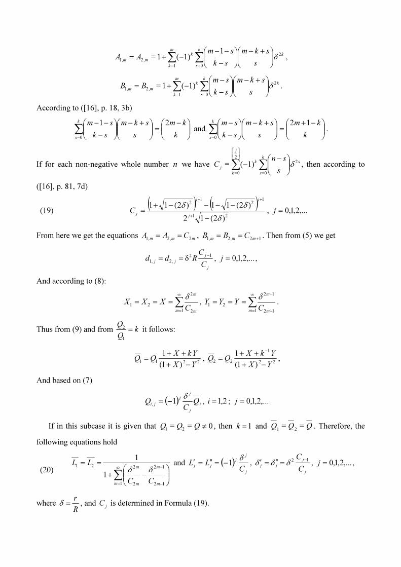
If for each non-negative whole number n we have s

s

kk

k

j

js

snC

2

0=0=

2

1)(= δ

−− ∑∑

, then according to

([16], p. 81, 7d)

(19) ( ) ( )

21

12

12

)2(12

)2(11)2(11

δ

δδ

−

−−−−+

=+

++

j

jj

jC , ,...2,1,0=j

From here we get the equations mmm

CAA2,2,1

== , 12,2,1 +

==mmm

CBB . Then from (5) we get

j

j

jjC

CRdd

12

,2,1δ

−

== , ,...2,1,0=j ,

And according to (8):

∑∞

=

===1 2

2

21

m m

m

CXXX

δ, ∑

∞

= −

−

===

1 12

12

21

m m

m

CYYY

δ.

Thus from (9) and from kQ

Q=

1

2 it follows:

2211

)1(

1

YX

YkXQQ

−+

++= ,

22

1

22

)1(

1

YX

YkXQQ

−+

++=

−

,

And based on (7)

( )i

j

jj

jiQ

CQ

δ1

,

−= , 2,1=i ; ,...2,1,0=j

If in this subcase it is given that 0==21

≠QQQ , then 1=k and QQQ ==21

. Therefore, the

following equations hold

(20) ∑∞

= −

−

−+

==

1 12

12

2

221

1

1

m m

m

m

m

CC

LLδδ

and ( )j

jj

jjC

LLδ

1−=′′=′ , j

j

jjC

C12 −

=′′=′ δδδ , ,...2,1,0=j ,

where R

r=δ , and

jC is determined in Formula (19).

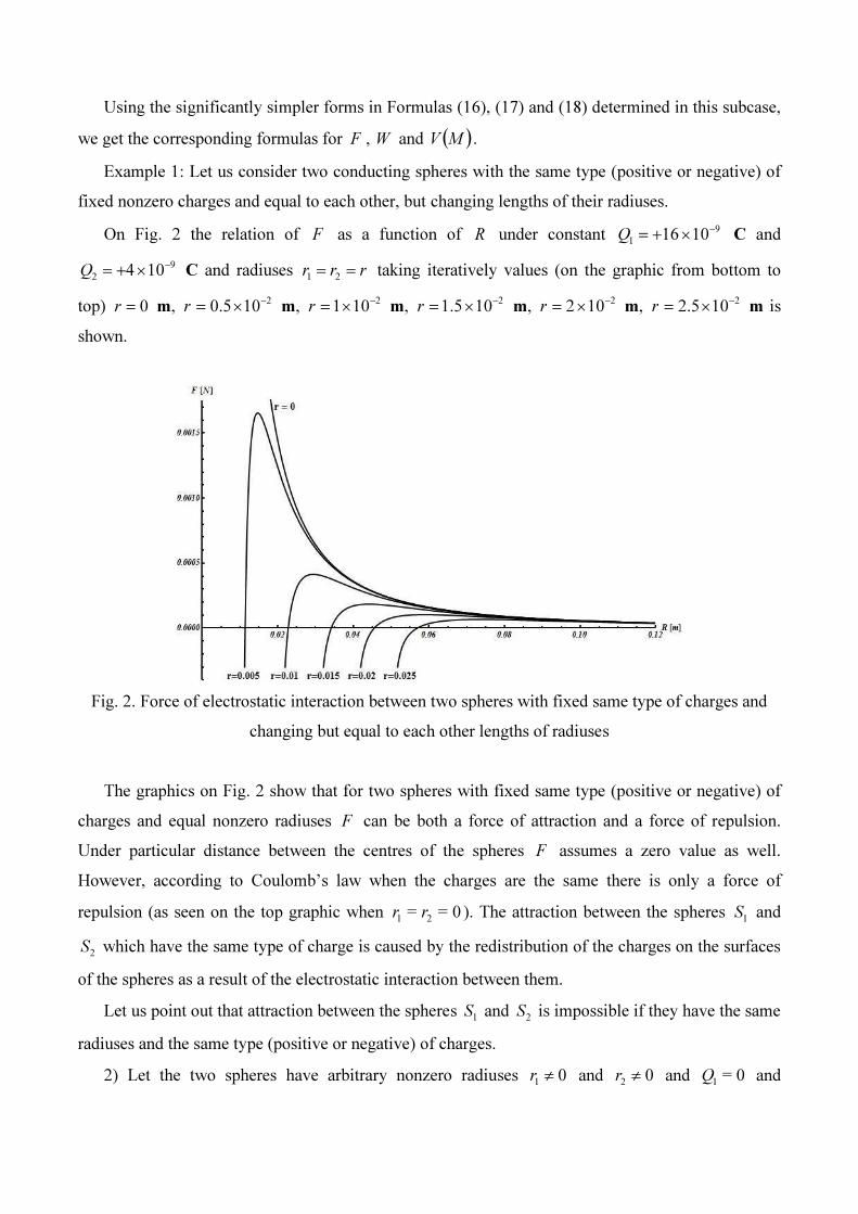
Using the significantly simpler forms in Formulas (16), (17) and (18) determined in this subcase,

we get the corresponding formulas for F , W and ( )MV .

Example 1: Let us consider two conducting spheres with the same type (positive or negative) of

fixed nonzero charges and equal to each other, but changing lengths of their radiuses.

On Fig. 2 the relation of F as a function of R under constant 9

11016

−

×+=Q C and

9

2104

−

×+=Q C and radiuses rrr ==21

taking iteratively values (on the graphic from bottom to

top) 0=r m, 2105.0

−

×=r m, 2101

−

×=r m, 2105.1

−

×=r m, 2102

−

×=r m, 2105.2

−

×=r m is

shown.

Fig. 2. Force of electrostatic interaction between two spheres with fixed same type of charges and

changing but equal to each other lengths of radiuses

The graphics on Fig. 2 show that for two spheres with fixed same type (positive or negative) of

charges and equal nonzero radiuses F can be both a force of attraction and a force of repulsion.

Under particular distance between the centres of the spheres F assumes a zero value as well.

However, according to Coulomb’s law when the charges are the same there is only a force of

repulsion (as seen on the top graphic when 0==21rr ). The attraction between the spheres

1S and

2S which have the same type of charge is caused by the redistribution of the charges on the surfaces

of the spheres as a result of the electrostatic interaction between them.

Let us point out that attraction between the spheres 1S and

2S is impossible if they have the same

radiuses and the same type (positive or negative) of charges.

2) Let the two spheres have arbitrary nonzero radiuses 01≠r and 0

2≠r and 0=

1Q and

0=2

≠QQ , i.e. one of the spheres is not charged. Then 0,1,1==mm

BA , 0,2≠

mA , 0

,2≠

mB ,

0==11YX , 0=

2≠XX and 0=

2≠YY . From Formula (9) we get

X

QYQ

+

=

11

, X

QQ

+

=

12

.

In this case we determine 0=1, jd and 0=

1, jQ and

jd2,

and j

Q2,

( ,...3,2,1=j ) respectively using

Formulas (5) and (7). Using these equations in Formulas (10), (11) and (12) we get respectively F ,

W and ( )MV .

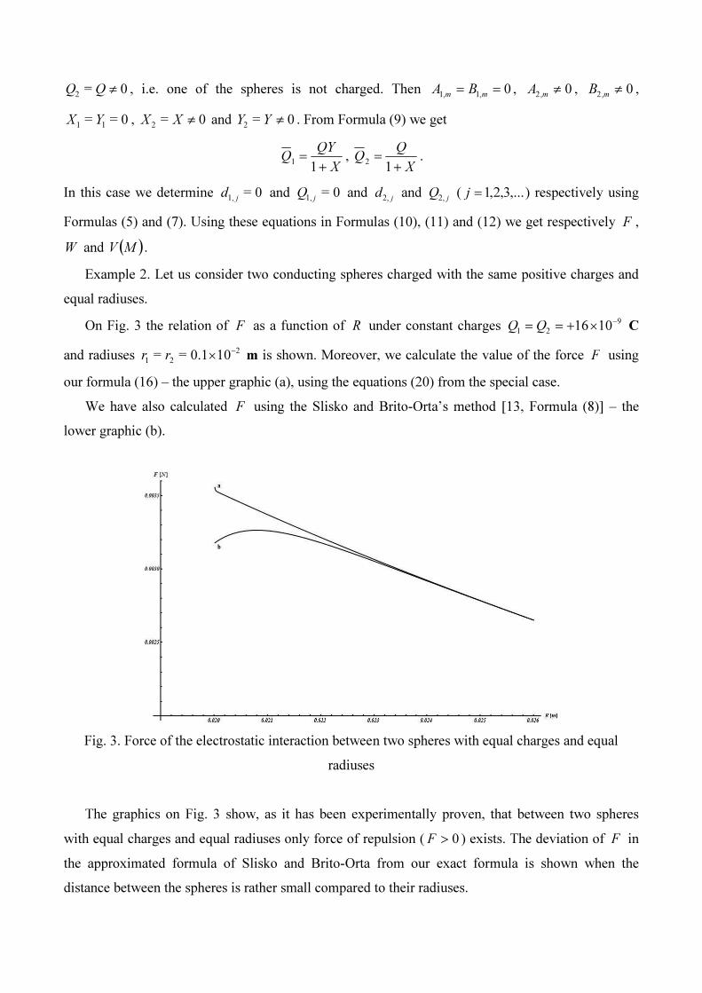
Example 2. Let us consider two conducting spheres charged with the same positive charges and

equal radiuses.

On Fig. 3 the relation of F as a function of R under constant charges 9

211016

−

×+== QQ C

and radiuses 2

21101.0==

−×rr m is shown. Moreover, we calculate the value of the force F using

our formula (16) – the upper graphic (a), using the equations (20) from the special case.

We have also calculated F using the Slisko and Brito-Orta’s method [13, Formula (8)] – the

lower graphic (b).

Fig. 3. Force of the electrostatic interaction between two spheres with equal charges and equal

radiuses

The graphics on Fig. 3 show, as it has been experimentally proven, that between two spheres

with equal charges and equal radiuses only force of repulsion ( 0>F ) exists. The deviation of F in

the approximated formula of Slisko and Brito-Orta from our exact formula is shown when the

distance between the spheres is rather small compared to their radiuses.

The graphics on Fig. 2 and Fig. 3 are achieved with the help of Wolfram Mathematica 7.0 and are

based on the formulas from Section 2.

3) Let us consider the case when 01≠= rr , 0

2=r , 0=

1Q , 0=

2≠QQ , i.e. we have uncharged

conducting sphere SS =1

and point charge Q situated out of it. Then R

r=δ=

1δ , 0=

2δ . From (5)

and (7) follows Rd2

1,2δ= and 0=

,2,1=

njdd , QQ δ−=

1,2, 0

,2,1==

njQQ ( ,...3,2,1=j ; ,...4,3,2=n ).

Based on Formulas (8) we get 0===121YXX and

R

rY =δ=2

and according to (9) δ=1

QQ ,

QQ =2

. Then from Formulas (10) and (11) we get

222

223

3

0

2

222

0

2

)(

)2(

4=

)1(

δ

4=

rR

Rrr

R

Q

R

QF

−

−

−−

πεδδ

πε,

22

3

2

0

2

2

0

2

4=

δ1

δδ

4=

rR

r

R

Q

R

QW

−−

−−

πεπε

.

The result for F is the same as the known for the size of the projecting of the force with which

the uncharged conducting sphere and a situated out of it point charge interact with each other [1, 10].

Under these conditions, according to (12)

( )

−+

1000

δ1

4=

bba

QMV

δ

πε.

This result is known for the potential, created by an uncharged conducting sphere and a point

electric charge, situated out of it [17].

4. Discussion

The formulas derived using an algebraic method for two charged conducting spheres with

arbitrary charges and radiuses are easily applicable. They give an analytical description of both the

force of the electrostatic interaction and the potential energy and the potential of the electrostatic

field. Our formulas summarise many of the results found by other researchers. Our results also yield

the fundamental Coulomb’s law. Moreover, our algebraic method does not have any electrostatic

constraints.

We compared the general analytical formulas we derived with already known results and

confirmed the correctness of our conclusions. For example, in the special case when we have spheres

with equal radiuses and charges the numerical values for the force F of the electrostatic interaction,

determined by Formula (8) in [13] approximately equals the values given by our Formula (16). This

equality does not hold when the distance between the spheres is rather small compared to their

radiuses because we can calculate an infinite number of interactions between the charges in the two

spheres. When we have uncharged conducting sphere and a point charge located outside of it our

formula for the force F is the same as the result in [1] and [10] and our formula for the potential V

is the same as the famous result in [17].

From Fig. 2 it is clear that only when the conducting spheres are far enough apart from each

other, the deviation of F from the corresponding value from Coulomb’s law for point charges 1Q

and 2

Q is very little. Moreover, our algebraic method gives (in Formulas (16), (17) and (18)) the

deviation of the values of F , W and V for charged conducting spheres from the corresponding

values 0

F , 0W and

0V for point charges. This deviation is caused by the redistribution of the charges

on the surfaces of the spheres caused by the electrostatic interaction between them. Based exactly on

that redistribution, two spheres with the same type of charges can attract each other.

6. Conclusion

Our method is also applicable for electrically conducting solid bodies, having a single centre of

symmetry. In that case we can consider such solid body to be an approximation of an equally

surfaced sphere, i.e. sphere having the same surface area and centre – the centre of symmetry of the

body. Such bodies are for example an ellipsoid, torus, as well as the five regular polyhedrons in the

three dimensional Euclidean space: tetrahedron, hexahedron (cube), octahedron, dodecahedron and

icosahedron.

Judging by the current publications the results in the paper are applicable not only to the

electrostatics, but also to fields like composite materials, suspension and others. We also apply these

results when considering the interactions between the nucleons in the cores of the atoms [18].

Acknowledgements

We would like to thank Pando Georgiev (PhD, DSci, Assoc. Research Scientist, Center for

Applied Optimization, ISE Department University of Florida) for the careful inspection of the

current work which confirmed our results.

The current research is done with the financial support of the Fund „Scientific Studies” of the

Bulgarian Ministry of Education, Youth and Science as part of the contract DTK 02/35.

References

[1] J. Maxwell, A Treatise on Electricity and Magnetism, vol. 1, Dover, 1954.

[2] E. Shpolski, Atomic Physics, vol. 2. Nauka, Moscow, 1984, (in Russian).

[3] V. Batygin, I. Toptygin, Problems in Electrodynamics, Academic Press Inc, 1978.

[4] W. Smythe, Static and Dynamic Electricity, McGraw-Hill, 1968.

[5] B. Budak, A. Samarskii, A. Tikhonov, A Collection of Problems in Mathematical Physics,

Dover Publications, 1988.

[6] H. van den Bosch, K. Ptasinski, P. Kerkhof, Two conducting spheres in a parallel electric

field, J. Appl. Phys. 78 (1995) 6345-6352.

[7] B. Djordjevic, J. Hеtherington, M. Thorpe, Spectral function for a conducting sheet

containing circular inclusions, Phys. Rev. B. 53 (1996) 14862-14871.

[8] Z. Jiang, Electrostatic interaction of two unequal conducting spheres in uniform electric field,

J. Electrostat. 58 (2003) 247-264.

[9] T. Jones, B. Rubin, Forces and torques on conducting particle chains, J. Electrostat. 21 (1988)

121-134.

[10] J. Jackson, Classical Electrodynamics, Wiley, 1998.

[11] J. Soules, Precise calculation of the electrostatic force between charged spheres including

induction effects, Am. J. Phys. 58 (1990) 1195-1199.

[12] C. Larson, E. Goss, A Coulomb’s law balance suitable for physics majors and nonscience

students, Am. J. Phys. 38, (1970) 1349–1352.

[13] J. Slisko, R. Brito-Orta, On approximate formulas for the electrostatic force between two

conducting spheres, Am. J. Phys. 66 (1998) 352-355.

[14] К. Кolikov, G. Кrustev, D. Ivanov, H. Кulina, On the electrostatic interaction between two

conductors with surfaces possessing center of symmetry, Scientific research of the Union of

Scientists in Bulgaria – Plovdiv, series B. Technics and Technologies XII (2008) 238-245 (in

Bulgarian).

[15] D. Halliday, R. Resnick, J. Walker, Fundamentals of Physics, Wiley, 2010.

[16] J. Riordan, Combinatorial Identities, Nauka, Moscow, 1982 (in Russian).

[17] R. Feynman, The Feynman Lectures on Physics: Exercises, Addison Wesley Publishing Co,

1964.

[18] К. Кolikov, D. Ivanov, G. Кrustev, Electromagnetic nature of the nuclear forces and a toroid

model of nucleons in atomic nuclei, Scientific research of the Union of Scientists in Bulgaria –

Plovdiv, series B. Nat. Sci. Humanities XIII (11-12 November 2010) 282-300.