electromagnetic theory - johnboccio.comjohnboccio.com/advanced/9-electromagnetictheory.pdf · the...
TRANSCRIPT
Electromagnetic Theory

Contents
1 Maxwell’s electrodynamics 11.1 Dynamical variables of electromagnetism 11.2 Maxwell’s equations and the Lorentz force 31.3 Conservation of charge 41.4 Conservation of energy 41.5 Conservation of momentum 61.6 Junction conditions 71.7 Potentials 101.8 Green’s function for Poisson’s equation 121.9 Green’s function for the wave equation 141.10 Summary 161.11 Problems 17
2 Electrostatics 212.1 Equations of electrostatics 212.2 Point charge 212.3 Dipole 222.4 Boundary-value problems: Green’s theorem 242.5 Laplace’s equation in spherical coordinates 282.6 Green’s function in the absence of boundaries 302.7 Dirichlet Green’s function for a spherical inner boundary 342.8 Point charge outside a grounded, spherical conductor 352.9 Ring of charge outside a grounded, spherical conductor 382.10 Multipole expansion of the electric field 402.11 Multipolar fields 422.12 Problems 45
3 Magnetostatics 473.1 Equations of magnetostatics 473.2 Circular current loop 473.3 Spinning charged sphere 493.4 Multipole expansion of the magnetic field 513.5 Problems 53
4 Electromagnetic waves in matter 554.1 Macroscopic form of Maxwell’s equations 55
4.1.1 Microscopic and macroscopic quantities 554.1.2 Macroscopic smoothing 564.1.3 Macroscopic averaging of the charge density 574.1.4 Macroscopic averaging of the current density 604.1.5 Summary — macroscopic Maxwell equations 61
4.2 Maxwell’s equations in the frequency domain 624.3 Dielectric constant 63
i
ii Contents
4.4 Propagation of plane, monochromatic waves 654.5 Propagation of wave packets 68
4.5.1 Description of wave packets 684.5.2 Propagation without dispersion 694.5.3 Propagation with dispersion 694.5.4 Gaussian wave packet 71
4.6 Problems 73
5 Electromagnetic radiation from slowly moving sources 755.1 Equations of electrodynamics 755.2 Plane waves 765.3 Spherical waves — the oscillating dipole 78
5.3.1 Plane versus spherical waves 785.3.2 Potentials of an oscillating dipole 795.3.3 Wave-zone fields of an oscillating dipole 815.3.4 Poynting vector of an oscillating dipole 835.3.5 Summary — oscillating dipole 84
5.4 Electric dipole radiation 845.4.1 Slow-motion approximation; near and wave zones 855.4.2 Scalar potential 855.4.3 Vector potential 875.4.4 Wave-zone fields 885.4.5 Energy radiated 905.4.6 Summary — electric dipole radiation 90
5.5 Centre-fed linear antenna 915.6 Classical atom 945.7 Magnetic-dipole and electric-quadrupole radiation 95
5.7.1 Wave-zone fields 965.7.2 Charge-conservation identities 985.7.3 Vector potential in the wave zone 995.7.4 Radiated power (magnetic-dipole radiation) 1005.7.5 Radiated power (electric-quadrupole radiation) 1015.7.6 Total radiated power 1025.7.7 Angular integrations 103
5.8 Pulsar spin-down 1035.9 Problems 105
6 Electrodynamics of point charges 1096.1 Lorentz transformations 1096.2 Fields of a uniformly moving charge 1126.3 Fields of an arbitrarily moving charge 114
6.3.1 Potentials 1156.3.2 Fields 1166.3.3 Uniform motion 1206.3.4 Summary 121
6.4 Radiation from an accelerated charge 1226.4.1 Angular profile of radiated power 1226.4.2 Slow motion: Larmor formula 1236.4.3 Linear motion 1246.4.4 Circular motion 1266.4.5 Synchrotron radiation 1276.4.6 Extremely relativistic motion 131
6.5 Radiation reaction 1326.6 Problems 135
Chapter 1
Maxwell’s electrodynamics
1.1 Dynamical variables of electromagnetism
The classical theory of the electromagnetic field, as formulated by Maxwell, involvesthe vector fields
E(t,x) ≡ electric field at position x and time t (1.1.1)
andB(t,x) ≡ magnetic field at position x and time t. (1.1.2)
We have two vectors at each position of space and at each moment of time. Thedynamical system is therefore much more complicated than in mechanics, in whichthere is a finite number of degrees of freedom. Here the number of degrees of freedomis infinite.
The electric and magnetic fields are produced by charges and currents. In aclassical theory these are best described in terms of a fluid picture in which thecharge and current distributions are imagined to be continuous (and not made ofpointlike charge carriers). Although this is not a true picture of reality, these con-tinuous distributions fit naturally within a classical treatment of electrodynamics.This will be our point of view here, but we shall see that the formalism is robustenough to also allow for a description in terms of point particles.
An element of charge is a macroscopically small (but microscopically large)portion of matter that contains a net charge. An element of charge is locatedat position x and has a volume dV . It moves with a velocity v that depends ontime and on position. The volume of a charge element must be sufficiently largethat it contains a macroscopic number of elementary charges, but sufficiently smallthat the density of charge within the volume is uniform to a high degree of accuracy.
In the mathematical description, an element of charge at position x is idealized asthe point x itself. The quantities that describe the charge and current distributionsare
ρ(t,x) ≡ density of charge at position x and time t, (1.1.3)
v(t,x) ≡ velocity of an element of charge at position x and time t,(1.1.4)
j(t,x) ≡ current density at position x and time t. (1.1.5)
We shall now establish the important relation
j = ρv. (1.1.6)
The current density j is defined by the statement
j · da ≡ current crossing an element of area da, (1.1.7)
1
2 Maxwell’s electrodynamics
θ
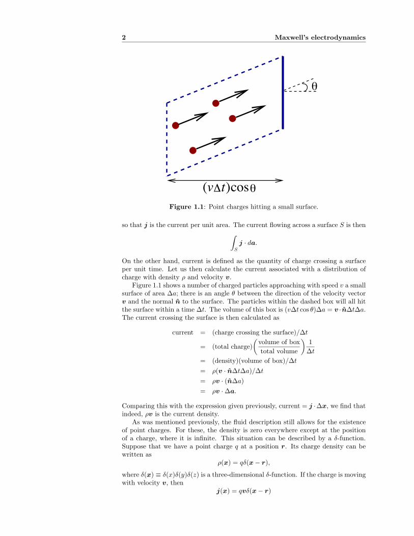
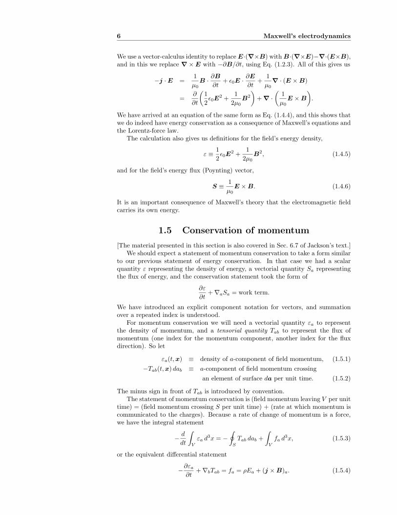
(v tΔ )cosθFigure 1.1: Point charges hitting a small surface.
so that j is the current per unit area. The current flowing across a surface S is then!
Sj · da.
On the other hand, current is defined as the quantity of charge crossing a surfaceper unit time. Let us then calculate the current associated with a distribution ofcharge with density ρ and velocity v.
Figure 1.1 shows a number of charged particles approaching with speed v a smallsurface of area ∆a; there is an angle θ between the direction of the velocity vectorv and the normal n to the surface. The particles within the dashed box will all hitthe surface within a time ∆t. The volume of this box is (v∆t cos θ)∆a = v · n∆t∆a.The current crossing the surface is then calculated as
current = (charge crossing the surface)/∆t
= (total charge)
"
volume of box
total volume
#
1
∆t
= (density)(volume of box)/∆t
= ρ(v · n∆t∆a)/∆t
= ρv · (n∆a)
= ρv · ∆a.
Comparing this with the expression given previously, current = j ·∆x, we find thatindeed, ρv is the current density.
As was mentioned previously, the fluid description still allows for the existenceof point charges. For these, the density is zero everywhere except at the positionof a charge, where it is infinite. This situation can be described by a δ-function.Suppose that we have a point charge q at a position r. Its charge density can bewritten as
ρ(x) = qδ(x − r),
where δ(x) ≡ δ(x)δ(y)δ(z) is a three-dimensional δ-function. If the charge is movingwith velocity v, then
j(x) = qvδ(x − r)
1.2 Maxwell’s equations and the Lorentz force 3
is the current density.More generally, let us have a collection of point charges qA at positions rA(t),
moving with velocities vA(t) = drA/dt. Then the charge and current densities ofthe charge distribution are given by
ρ(t,x) =$
A
qAδ%
x − rA(t)&
(1.1.8)
andj(t,x) =
$
A
qAvA(t)δ%
x − rA(t)&
. (1.1.9)
Each qA is the integral of ρ(t,x) over a volume VA that encloses this charge but noother:
qA =
!
VA
ρ(t,x) d3x, (1.1.10)
where d3x ≡ dxdydz. The total charge of the distribution is obtained by integratingthe density over all space:
Q ≡!
ρ(t,x) d3x =$
A
qA. (1.1.11)
1.2 Maxwell’s equations and the Lorentz force
The four Maxwell equations determine the electromagnetic field once the chargeand current distributions are specified. They are given by
∇ · E =1
ϵ0ρ, (1.2.1)
∇ · B = 0, (1.2.2)
∇ × E = −∂B
∂t, (1.2.3)
∇ × B = µ0j + ϵ0µ0∂E
∂t. (1.2.4)
Here, ϵ0 and µ0 are constants, and ∇ = (∇x,∇y,∇z) is the gradient operatorof vector calculus (with the obvious notation ∇xf = ∂f/∂x for any function f).The Maxwell equations state that the electric field is produced by charges andtime-varying magnetic fields, while the magnetic field is produced by currents andtime-varying electric fields. Maxwell’s equations can also be presented in integralform, by invoking the Gauss and Stokes theorems of vector calculus.
The Lorentz-force law determines the motion of the charges once the electro-magnetic field is specified. Let
f(t,x) ≡ force density at position x and time t, (1.2.5)
where the force density is defined to be the net force acting on an element of chargeat x divided by the volume of this charge element. The statement of the Lorentz-force law is then
f = ρE + j × B = ρ%
E + v × B&
. (1.2.6)
The net force F acting on a volume V of the charge distribution is the integral ofthe force density over this volume:
F (t, V ) =
!
Vf(t,x) d3x. (1.2.7)
4 Maxwell’s electrodynamics
For a single point charge we have ρ = qδ(x−r), j = qvδ(x−r), and the total forcebecomes
F = q'
E(r) + v × B(r)(
.
Here the fields are evaluated at the charge’s position. This is the usual expressionfor the Lorentz force, but the definition of Eq. (1.2.6) is more general.
Taken together, the Maxwell equations and the Lorentz-force law determine thebehaviour of the charge and current distributions, and the evolution of the electricand magnetic fields. Those five equations summarize the complete theory of classicalelectrodynamics. Every conceivable phenomenon involving electromagnetism can bepredicted from them.
1.3 Conservation of charge
One of the most fundamental consequences of Maxwell’s equations is that charge islocally conserved: charge can move around but it cannot be destroyed nor created.
Consider a volume V bounded by a two-dimensional surface S. Charge conser-vation means that the rate of decrease of charge within V must be equal to thetotal current flowing across S:
−d
dt
!
Vρ d3x =
)
Sj · da. (1.3.1)
Local charge conservation means that this statement must be true for any volumeV , however small or large. We may use Gauss’ theorem to turn Eq. (1.3.1) into adifferential statement. For any smooth vector field u within V we have
!
V∇ · u d3x =
)
Su · da.
The right-hand side of Eq. (1.3.1) can thus be written as*
V ∇ · j d3x, while theleft-hand side is equal to −
*
V (∂ρ/∂t) d3x. Equality of the two sides for arbitraryvolumes V implies
∂ρ
∂t+ ∇ · j = 0. (1.3.2)
This is the differential statement of local charge conservation, and we would like toprove that this comes as a consequence of Maxwell’s equations.
To establish this we first differentiate Eq. (1.2.1) with respect to time to obtain
∂ρ
∂t= ϵ0∇ ·
∂E
∂t,
where we have exchanged the order with which we take derivatives of the electricfield. If we now use Eq. (1.2.4) to eliminate the electric field, we get
∂ρ
∂t=
1
µ0∇ · (∇ × B) − ∇ · j.
The first term on the right-hand side vanishes identically (the divergence of a curl isalways zero) and we arrive at Eq. (1.3.2). We have therefore established that localcharge conservation is a consequence of Maxwell’s equations.
1.4 Conservation of energy
[The material presented in this section is also covered in Sec. 6.7 of Jackson’s text.]
1.4 Conservation of energy 5
Other conservation statements follow from Maxwell’s equations and the Lorentz-force law. In this section we formulate and derive a statement of energy conser-vation. In the next section we will consider the conservation of linear momentum.It is also possible to prove conservation of angular momentum, but we shall notpursue this here.
Conservation of energy is one of the most fundamental principle of physics, andMaxwell’s electrodynamics must be compatible with it. A statement of local energyconservation can be patterned after our previous statement of charge conservation.Let
ε(t,x) ≡ electromagnetic field energy density, (1.4.1)
S(t,x) · da ≡ field energy crossing an element of
surface da per unit time. (1.4.2)
So ε is analogous to charge density, and S (which is known as Poynting’s vector),is analogous to current density.
If electromagnetic field energy were locally conserved, we would write the state-ment
−d
dt
!
Vε d3x =
)
SS · da,
which is analogous to Eq. (1.3.1). But we should not expect field energy to beconserved, and this statement is not correct. The reason is that the field does workon the charge distribution, and this takes energy away from the field. This energygoes to the charge distribution, and total energy is conserved. A correct statementof energy conservation would therefore be (field energy leaving V per unit time) =(field energy crossing S per unit time) + (work done on charges within V per unittime). To figure out what the work term should be, consider an element of chargewithin V . It moves with a velocity v and the net force acting on it is
f dV = ρ(E + v × B) dV.
While the element undergoes a displacement dx, the force does a quantity of workequal to f · dx dV . The work done per unit time is then f · v dV = ρE · v dV =j ·E dV . Integrating this over V gives the total work done on the charges containedin V , per unit time. The correct statement of energy conservation must thereforehave the form
−d
dt
!
Vε d3x =
)
SS · da +
!
Vj · E d3x. (1.4.3)
In differential form, this is
∂ε
∂t+ ∇ · S = −j · E. (1.4.4)
This last equation must be derivable from Maxwell’s equations, which have notyet been involved. And indeed, the derivation should provide expressions for thequantities ε and S. What we have at this stage is an educated guess for a correctstatement of energy conservation, but Eq. (1.4.4) has not yet been derived nor thethe quantities ε and S properly defined in terms of field variables. Now the hardwork begins.
We start with the right-hand side of Eq. (1.4.4) and eliminate j in favour of fieldvariables using Eq. (1.2.4). This gives
−j · E = −1
µ0E · (∇ × B) + ϵ0E ·
∂E
∂t.
6 Maxwell’s electrodynamics
We use a vector-calculus identity to replace E·(∇×B) with B·(∇×E)−∇·(E×B),and in this we replace ∇ × E with −∂B/∂t, using Eq. (1.2.3). All of this gives us
−j · E =1
µ0B ·
∂B
∂t+ ϵ0E ·
∂E
∂t+
1
µ0∇ · (E × B)
=∂
∂t
"
1
2ϵ0E
2 +1
2µ0B2
#
+ ∇ ·"
1
µ0E × B
#
.
We have arrived at an equation of the same form as Eq. (1.4.4), and this shows thatwe do indeed have energy conservation as a consequence of Maxwell’s equations andthe Lorentz-force law.
The calculation also gives us definitions for the field’s energy density,
ε ≡1
2ϵ0E
2 +1
2µ0B2, (1.4.5)
and for the field’s energy flux (Poynting) vector,
S ≡1
µ0E × B. (1.4.6)
It is an important consequence of Maxwell’s theory that the electromagnetic fieldcarries its own energy.
1.5 Conservation of momentum
[The material presented in this section is also covered in Sec. 6.7 of Jackson’s text.]We should expect a statement of momentum conservation to take a form similar
to our previous statement of energy conservation. In that case we had a scalarquantity ε representing the density of energy, a vectorial quantity Sa representingthe flux of energy, and the conservation statement took the form of
∂ε
∂t+ ∇aSa = work term.
We have introduced an explicit component notation for vectors, and summationover a repeated index is understood.
For momentum conservation we will need a vectorial quantity εa to representthe density of momentum, and a tensorial quantity Tab to represent the flux ofmomentum (one index for the momentum component, another index for the fluxdirection). So let
εa(t,x) ≡ density of a-component of field momentum, (1.5.1)
−Tab(t,x) dab ≡ a-component of field momentum crossing
an element of surface da per unit time. (1.5.2)
The minus sign in front of Tab is introduced by convention.The statement of momentum conservation is (field momentum leaving V per unit
time) = (field momentum crossing S per unit time) + (rate at which momentum iscommunicated to the charges). Because a rate of change of momentum is a force,we have the integral statement
−d
dt
!
Vεa d3x = −
)
STab dab +
!
Vfa d3x, (1.5.3)
or the equivalent differential statement
−∂εa
∂t+ ∇bTab = fa = ρEa + (j × B)a. (1.5.4)
1.6 Junction conditions 7
We now would like to derive this from Maxwell’s equations, and discover the iden-tities of the vector εa and the tensor Tab.
We first use Eqs. (1.2.1) and (1.2.4) to eliminate ρ and j from Eq. (1.5.4):
f = (ϵ0∇ · E)E +
"
1
µ0∇ × B − ϵ0
∂E
∂t
#
× B
= ϵ0(∇ · E)E +1
µ0(∇ · B)B +
1
µ0(∇ × B) × B
− ϵ0∂
∂t(E × B) + ϵ0E ×
∂B
∂t,
where to go from the first to the second line we have inserted a term involving∇ · B = 0 and allowed the time derivative to operate on E × B. The next step isto use Eq. (1.2.3) to replace ∂B/∂t with −∇ × E. Collecting terms, this gives
f = −ϵ0∂
∂t(E×B)+ ϵ0
'
(∇ ·E)E−E× (∇×E)(
+1
µ0
'
(∇ ·B)B−B× (∇×B)(
.
To proceed we invoke the vector-calculus identity 12∇(u·u) = (u·∇)u+u×(∇×u),
where u stands for any vector field. We use this to clean up the quantities withinsquare brackets. For example,
(∇ · E)E − E × (∇ × E) = (∇ · E)E + (E · ∇)E −1
2∇(E · E).
In components, the right-hand side reads
(∇bEb)Ea + (Eb∇b)Ea −1
2∇aE2 = Ea∇bEb + Eb∇bEa −
1
2δab∇bE
2
= ∇b
"
EaEb −1
2δabE
2
#
.
Doing the same for the bracketed terms involving the magnetic field, we arrive at
fa = −ϵ0∂
∂t(E × B)a + ϵ0∇b
"
EaEb −1
2δabE
2
#
+1
µ0∇b
"
BaBb −1
2δabB
2
#
.
This has the form of Eq. (1.5.4) and we conclude that momentum conservation doesindeed follow from Maxwell’s equations and the Lorentz-force law.
Our calculation also tells us that the field’s momentum density is given by
εa ≡ ϵ0(E × B)a, (1.5.5)
and that the field’s momentum flux tensor is
Tab = ϵ0
"
EaEb −1
2δabE
2
#
+1
µ0
"
BaBb −1
2δabB
2
#
. (1.5.6)
Notice that the momentum density is proportional to the Poynting vector: ε =ϵ0µ0S. This means that the field’s momentum points in the same direction as theflow of energy, and that these quantities are related by a constant factor of ϵ0µ0.
1.6 Junction conditions
[The material presented in this section is also covered in Sec. I.5 of Jackson’s text.]Maxwell’s equations determine how the electric and magnetic fields must be
joined at an interface. The interface might be just a mathematical boundary (in
8 Maxwell’s electrodynamics
which case nothing special should happen), or it might support a surface layerof charge and/or current. Our task in this section is to formulate these junctionconditions.
To begin, we keep things simple by supposing that the interface is the x-y planeat z = 0 — a nice, flat surface. If the interface supports a charge distribution, thenthe charge density must have the form
ρ(t,x) = ρ+(t,x)θ(z) + ρ−(t,x)θ(−z) + σ(t, x, y)δ(z), (1.6.1)
where ρ+ is the charge density above the interface (in the region z > 0), ρ− thecharge density below the interface (in the region z < 0), and σ is the surface densityof charge (charge per unit surface area) supported by the interface.
We have introduced the Heaviside step function θ(z), which is equal to 1 ifz > 0 and 0 otherwise, and the Dirac δ-function, which is such that
*
f(z)δ(z) dz =f(0) for any smooth function f(z). These distributions (also known as generalizedfunctions) are related by the identities
d
dzθ(z) = δ(z),
d
dzθ(−z) = −δ(z). (1.6.2)
As for any distributional identity, these relations can be established by integratingboth sides against a test function f(z). (Test functions are required to be smoothand to fall off sufficiently rapidly as z → ±∞.) For example,
! ∞
−∞
dθ(z)
dzf(z) dz = −
! ∞
−∞θ(z)
df(z)
dzdz
= −! ∞
0df
= f(0),
and this shows that dθ(z)/dz is indeed distributionally equal to δ(z). You can showsimilarly that f(z)δ(z) = f(0)δ(z) and f(z)δ′(z) = f(0)δ′(z) − f ′(0)δ(z) are validdistributional identities (a prime indicates differentiation with respect to z).
If the interface at z = 0 also supports a current distribution, then the currentdensity must have the form
j(t,x) = j+(t,x)θ(z) + j−(t,x)θ(−z) + K(t, x, y)δ(z), (1.6.3)
where j+ is the current density above the interface, j− the current density belowthe interface, and K is the surface density of current (charge per unit time and unitlength) supported by the interface.
We now would like to determine how E and B behave across the interface. Wecan express the fields as
E(t,x) = E+(t,x)θ(z) + E−(t,x)θ(−z),
(1.6.4)
B(t,x) = B+(t,x)θ(z) + B−(t,x)θ(−z),
in an obvious notation; for example, E+ is the electric field above the interface. Wewill see that these fields are solutions to Maxwell’s equations with sources given byEqs. (1.6.1) and (1.6.3). To prove this we need simply substitute Eq. (1.6.4) intoEqs. (1.2.1)–(1.2.4). Differentiating the coefficients of θ(±z) is straightforward, butwe must also differentiate the step functions. For this we use Eq. (1.6.2) and write
∇θ(±z) = ±δ(z)z,
1.6 Junction conditions 9
where z is a unit vector that points in the z direction.A straightforward calculation gives
∇ · E =%
∇ · E+
&
θ(z) +%
∇ · E−
&
θ(−z) + z ·%
E+ − E−
&
δ(z),
∇ × E =%
∇ × E+
&
θ(z) +%
∇ × E−
&
θ(−z) + z ×%
E+ − E−
&
δ(z),
∇ · B =%
∇ · B+
&
θ(z) +%
∇ · B−
&
θ(−z) + z ·%
B+ − B−
&
δ(z),
∇ × B =%
∇ × B+
&
θ(z) +%
∇ × B−
&
θ(−z) + z ×%
B+ − B−
&
δ(z).
Substituting Eq. (1.6.1) and the expression for ∇ · E into the first of Maxwell’sequations, ∇ · E = ρ/ϵ0, reveals that E± is produced by ρ± and that the surfacecharge distribution creates a discontinuity in the normal component of the electricfield:
z ·%
E+ − E−
&+
+
z=0=
1
ϵ0σ. (1.6.5)
Substituting the expression for ∇·B into the second of Maxwell’s equations, ∇·B =0, reveals that B± satisfies this equation on both sides of the interface and that thenormal component of the magnetic field must be continuous:
z ·%
B+ − B−
&+
+
z=0= 0. (1.6.6)
Substituting Eq. (1.6.4) and the expression for ∇ × E into the third of Maxwell’sequations, ∇×E = −∂B/∂t, reveals that E± and B± satisfy this equation on bothsides of the interface and that the tangential (x and y) components of the electricmust also be continuous:
z ×%
E+ − E−
&+
+
z=0= 0. (1.6.7)
Finally, substituting Eqs. (1.6.3), (1.6.4), and the expression for ∇ × B into thefourth of Maxwell’s equations, ∇ × B = µ0j + ϵ0µ0∂E/∂t, reveals that B± isproduced by j± and that the surface current creates a discontinuity in the tangentialcomponents of the magnetic field:
z ×%
B+ − B−
&+
+
z=0= µ0K. (1.6.8)
Equations (1.6.5)–(1.6.8) tell us how the fields E± and B± are to be joined at aplanar interface.
It is not difficult to generalize this discussion to an interface of arbitrary shape.All that is required is to change the argument of the step and δ functions from zto s(x), where s is the distance from the interface in the direction normal to theinterface; this is positive above the interface and negative below the interface. Then∇s = n, the interface’s unit normal, replaces z in the preceding equations. If E+,B+ are the fields just above the interface, and E−, B− the fields just below theinterface, then the general junction conditions are
n ·%
E+ − E−
&
=1
ϵ0σ, (1.6.9)
n ·%
B+ − B−
&
= 0, (1.6.10)
n ×%
E+ − E−
&
= 0, (1.6.11)
n ×%
B+ − B−
&
= µ0K. (1.6.12)
Here, σ is the surface charge density on the general interface, and K is the surfacecurrent density. It is understood that the normal vector points from the minus sideto the plus side of the interface.
10 Maxwell’s electrodynamics
1.7 Potentials
[The material presented in this section is also covered in Secs. 6.2 and 6.3 of Jack-son’s text.]
The Maxwell equation ∇ ·B = 0 and the mathematical identity ∇ ·(∇×A) = 0imply that the magnetic field can be expressed as the curl of a vector potentialA(t,x):
B = ∇ × A. (1.7.1)
Suppose that B is expressed in this form. Then the other inhomogeneous Maxwellequation, ∇ × E + ∂B/∂t = 0, can be cast in the form
∇ ×"
E +∂A
∂t
#
= 0.
This, together with the mathematical identity ∇×(∇Φ) = 0, imply that E+∂A/∂tcan be expressed as the divergence of a scalar potential Φ(t,x):
E = −∂A
∂t− ∇Φ; (1.7.2)
the minus sign in front of ∇Φ is conventional.Introducing the scalar and vector potentials eliminates two of the four Maxwell
equations. The remaining two equations will give us equations to be satisfied by thepotentials. Solving these is often much simpler than solving the original equations.An issue that arises is whether the scalar and vector potentials are unique: WhileE and B can both be obtained uniquely from Φ and A, is the converse true? Theanswer is in the negative — the potentials are not unique.
Consider the following gauge transformation of the potentials:
Φ → Φnew = Φ −∂f
∂t, (1.7.3)
A → Anew = A + ∇f, (1.7.4)
in which f(t,x) is an arbitrary function of space and time. We wish to show thatthis transformation leaves the fields unchanged:
Enew = E, Bnew = B. (1.7.5)
This implies that the potentials are not unique: they can be redefined at will by agauge transformation. The new electric field is given by
Enew = −∂Anew
∂t− ∇Φnew
= −∂
∂t
,
A + ∇f-
− ∇
"
Φ −∂f
∂t
#
= E −∂
∂t∇f + ∇
∂f
∂t;
the last two terms cancel out and we have established the invariance of the electricfield. On the other hand, the new magnetic field is given by
Bnew = ∇ × Anew
= ∇ ×%
A + ∇f&
= B + ∇ × (∇f);
the last term is identically zero and we have established the invariance of the mag-netic field. We will use the gauge invariance of the electromagnetic field to simplifythe equations to be satisfied by the scalar and vector potentials.
1.7 Potentials 11
To derive these we start with Eq. (1.2.1) and cast it in the form
1
ϵ0ρ = ∇ · E = ∇ ·
"
−∂A
∂t− ∇Φ
#
= −∂
∂t∇ · A −∇2Φ,
or1
ϵ0ρ = ϵ0µ0
∂2Φ
∂t2−∇2Φ −
∂
∂t
"
∇ · A + ϵ0µ0∂Φ
∂t
#
, (1.7.6)
where, for reasons that will become clear, we have added and subtracted a termϵ0µ0∂2Φ/∂t2. Similarly, we re-express Eq. (1.2.4) in terms of the potentials:
µ0j = ∇ × B − ϵ0µ0∂E
∂t
= ∇ × (∇ × A) − ϵ0µ0∂
∂t
"
−∂A
∂t− ∇Φ
#
= ∇(∇ · A) −∇2A + ϵ0µ0∂2A
∂t2+ ϵ0µ0∇
∂Φ
∂t,
where we have used a vector-calculus identity to eliminate ∇ × (∇ × A). We haveobtained
µ0j = ϵ0µ0∂2A
∂t2−∇2A + ∇
"
∇ · A + ϵ0µ0∂Φ
∂t
#
. (1.7.7)
Equations (1.7.6) and (1.7.7) govern the behaviour of the potentials; they are equiv-alent to the two Maxwell equations that remain after imposing Eqs. (1.7.1) and(1.7.2).
These equations would be much simplified if we could demand that the potentialssatisfy the supplementary condition
∇ · A + ϵ0µ0∂Φ
∂t= 0. (1.7.8)
This is known as the Lorenz gauge condition, and as we shall see below, it canalways be imposed by redefining the potentials according to Eqs. (1.7.3) and (1.7.4)with a specific choice of function f(t,x). When Eq. (1.7.8) holds we observe thatthe equations for Φ and A decouple from one another, and that they both take theform of a wave equation:
"
−1
c2
∂2
∂t2+ ∇2
#
Φ(t,x) = −1
ϵ0ρ(t,x), (1.7.9)
"
−1
c2
∂2
∂t2+ ∇2
#
A(t,x) = −µ0j(t,x), (1.7.10)
where
c ≡1
√ϵ0µ0
(1.7.11)
is the speed with which the waves propagate; this is numerically equal to the speedof light in vacuum.
To see that the Lorenz gauge condition can always be imposed, imagine thatwe are given potentials Φold and Aold that do not satisfy the gauge condition. Weknow that we can transform them according to Φold → Φ = Φold − ∂f/∂t andAold → A = Aold +∇f , and we ask whether it is possible to find a function f(t,x)such that the new potentials Φ and A will satisfy Eq. (1.7.8). The answer is in theaffirmative: If Eq. (1.7.8) is true then
0 = ∇ · A + ϵ0µ0∂Φ
∂t
12 Maxwell’s electrodynamics
= ∇ ·%
Aold + ∇f&
+ ϵ0µ0∂
∂t
"
Φold −∂f
∂t
#
= ∇ · Aold + ϵ0µ0∂Φold
∂t− ϵ0µ0
∂2f
∂t2+ ∇2f,
and we see that the Lorenz gauge condition is satisfied if f(t,x) is a solution to thewave equation
"
−1
c2
∂2
∂t2+ ∇2
#
f = −∇ · Aold − ϵ0µ0∂Φold
∂t.
Such an equation always admits a solution, and we conclude that the Lorenz gaugecondition can always be imposed. (Notice that we do not need to solve the waveequation for f ; all we need to know is that solutions exist.)
To summarize, we have found that the original set of four Maxwell equations forthe fields E and B can be reduced to the two wave equations (1.7.9) and (1.7.10) forthe potentials Φ and A, supplemented by the Lorenz gauge condition of Eq. (1.7.8).Once solutions to these equations have been found, the fields can be constructedwith Eqs. (1.7.1) and (1.7.2). Introducing the potentials has therefore dramaticallyreduced the complexity of the equations, and correspondingly increased the ease offinding solutions.
In time-independent situations, the fields and potentials no longer depend on t,and the foregoing equations reduce to
∇2Φ(x) = −1
ϵ0ρ(x), (1.7.12)
∇2A(x) = −µ0j(x), (1.7.13)
as well as E = −∇Φ and B = ∇ × A. The Lorenz gauge condition reduces to∇ · A = 0 (also known as the Coulomb gauge condition), and the potentials nowsatisfy Poisson’s equation.
1.8 Green’s function for Poisson’s equation
[The material presented in this section is also covered in Sec. 1.7 of Jackson’s text.]We have seen in the preceding section that the task of solving Maxwell’s equa-
tions can be reduced to the simpler task of solving two wave equations. For time-independent situations, the wave equation becomes Poisson’s equation. In this andthe next section we will develop some of the mathematical tools needed to solvethese equations.
We begin in this section with the mathematical problem of solving a genericPoisson equation of the form
∇2ψ(x) = −4πf(x), (1.8.1)
where ψ(x) is the potential, f(x) a prescribed source function, and where a factorof 4π was inserted for later convenience.
To construct the general solution to this equation we shall first find a Green’sfunction G(x,x′) that satisfies a specialized form of Poisson’s equation:
∇2G(x,x′) = −4πδ(x − x′), (1.8.2)
where δ(x − x′) is a three-dimensional Dirac δ-function; the source point x′ isarbitrary. It is easy to see that if we have such a Green’s function at our disposal,then the general solution to Eq. (1.8.1) can be expressed as
ψ(x) = ψ0(x) +
!
G(x,x′)f(x′) d3x′, (1.8.3)
1.8 Green’s function for Poisson’s equation 13
where ψ0(x) is a solution to the inhomogeneous (Laplace) equation,
∇2ψ0(x) = 0. (1.8.4)
This assertion is proved by substituting Eq. (1.8.3) into the left-hand side of Eq. (1.8.1),and using Eqs. (1.8.2) and (1.8.4) to show that the result is indeed equal to −4πf(x).
In Eq. (1.8.3), the role of the integral is to account for the source term inEq. (1.8.1). The role of ψ0(x) is to enforce boundary conditions that we might wishto impose on the potential ψ(x). In the absence of such boundary conditions, ψ0
can simply be set equal to zero. Methods to solve boundary-value problems will beintroduced in the next chapter.
To construct the Green’s function we first argue that G(x,x′) can depend onlyon the difference x−x′; this follows from the fact that the source term depends onlyon x − x′, and the requirement that the Green’s function must be invariant undera translation of the coordinate system. We then express G(x,x′) as the Fouriertransform of a function G(k):
G(x,x′) =1
(2π)3
!
G(k)eik·(x−x′) d3k, (1.8.5)
where k is a vector in reciprocal space; this expression incorporates our assumptionthat G(x,x′) depends only on x − x′. Recalling that the three-dimensional δ-function can be represented as
δ(x − x′) =1
(2π)3
!
eik·(x−x′) d3k, (1.8.6)
we see that Eq. (1.8.2) implies k2G(k) = 4π, so that Eq. (1.8.6) becomes
G(x,x′) =4π
(2π)3
!
eik·(x−x′)
k2d3k. (1.8.7)
We must now evaluate this integral.To do this it is convenient to switch to spherical coordinates in reciprocal space,
defining a radius k and angles θ and φ by the relations kx = k sin θ cos φ, ky =k sin θ sin φ, and kz = k cos θ. In these coordinates the volume element is d3k =k2 sin θ dkdθdφ. For convenience we orient the coordinate system so that the kz
axis points in the direction of R ≡ x − x′. We then have k · R = kR cos θ, whereR ≡ |R| is the length of the vector R. All this gives
G(x,x′) =1
2π2
! ∞
0dk
! π
0dθ
! 2π
0dφ eikR cos θ sin θ.
Integration over dφ is trivial, and the θ integral can easily be evaluated by usingµ = cos θ as an integration variable:
! π
0eikR cos θ sin θ dθ =
! 1
−1eikRµ dµ =
2 sin kR
kR.
We now have
G(x,x′) =2
π
! ∞
0
sin kR
kRdk =
2
πR
! ∞
0
sin ξ
ξdξ,
where we have switched to ξ = kR. The remaining integral can easily be evaluatedby contour integration (or simply by looking it up in tables of integrals); it is equalto π/2.
14 Maxwell’s electrodynamics
Our final result is therefore
G(x,x′) =1
|x − x′|; (1.8.8)
the Green’s function for Poisson’s equation is simply the reciprocal of the distancebetween x and x′. The general solution to Poisson’s equation is then
ψ(x) = ψ0(x) +
!
f(x′)
|x − x′|d3x′. (1.8.9)
The meaning of this equation is that apart from the term ψ0, the potential at x isbuilt by summing over source contributions from all relevant points x′ and dividingby the distance between x and x′. Notice that in Eq. (1.8.8) we have recovered afamiliar result: the potential of a point charge at x′ goes like 1/R.
1.9 Green’s function for the wave equation
[The material presented in this section is also covered in Sec. 6.4 of Jackson’s text.]We now turn to the mathematical problem of solving the wave equation,
!ψ(t,x) = −4πf(t,x), (1.9.1)
for a time-dependent potential ψ produced by a prescribed source f ; we have intro-duced the wave, or d’Alembertian, differential operator
! ≡ −1
c2
∂2
∂t2+ ∇2. (1.9.2)
For this purpose we seek a Green’s function G(t,x; t′,x′) that satisfies
!G(t,x; t′,x′) = −4πδ(t − t′)δ(x − x′). (1.9.3)
In terms of this the general solution to Eq. (1.9.2) can be expressed as
ψ(t,x) = ψ0(t,x) +
! !
G(t,x; t′,x′)f(t′,x′) dt′d3x′, (1.9.4)
where ψ0(t,x) is a solution to the homogeneous wave equation,
!ψ0(t,x) = 0. (1.9.5)
That the potential of Eq. (1.9.4) does indeed solve Eq. (1.9.1) can be verified bydirect substitution.
To construct the Green’s function we Fourier transform it with respect to time,
G(t,x; t′,x′) =1
2π
!
G(ω;x,x′)e−iω(t−t′) dω, (1.9.6)
and we represent the time δ-function as
δ(t − t′) =1
2π
!
e−iω(t−t′) dω. (1.9.7)
Substituting these expressions into Eq. (1.9.3) yields'
∇2 + (ω/c)2(
G(ω;x,x′) = −4πδ(x − x′), (1.9.8)
which is a generalized form of Eq. (1.8.2). From this comparison we learn thatG(0;x,x′) = 1/|x − x′|.
1.9 Green’s function for the wave equation 15
At this stage we might proceed as in Sec. 1.8 and Fourier transform G(ω;x,x′)with respect to the spatial variables. This would eventually lead to
G(ω;x,x′) =4π
(2π)3
!
eik·(x−x′)
k2 − (ω/c)2d3k,
which is a generalized form of Eq. (1.8.7). This integral, however, is not defined,because of the singularity at k2 = (ω/c)2. We shall therefore reject this method ofsolution. (There are ways of regularizing the integral so as to obtain a meaningfulanswer. One method involves deforming the contour of the ω integration so as toavoid the poles. This is described in Sec. 12.11 of Jackson’s text.)
We can anticipate that for ω = 0, G will be of the form
G(ω;x,x′) =g(ω, |x − x′|)
|x − x′|, (1.9.9)
with g representing a function that stays nonsingular when the second argument,R ≡ |x − x′|, approaches zero. That G should depend on the spatial variablesthrough R only can be motivated on the grounds that three-dimensional space isboth homogeneous (so that G can only depend on the vector R ≡ x − x′) andisotropic (so that only the length of the vector matters, and not its direction). ThatG should behave as 1/R when R is small is justified by the following discussion.
Take Eq. (1.9.8) and integrate both sides over a sphere of small radius ε centeredat x′. Since ∇2G = ∇ · ∇G, we can use Gauss’ theorem to get
)
R=ε
%
∇G · R&
da + (ω/c)2!
R<εG d3x = −4π,
where R = R/R. In this equation, the volume integral is of order Gε3 and itcontributes nothing in the limit ε → 0, unless G happens to be as singular as 1/ε3.The surface integral, on the other hand, is equal to
4πε2 dG
dR
+
+
+
+
R=ε
.
If G were to behave as 1/ε3, then dG/dR would be of order 1/ε4, the surface integralwould contribute a term of order 1/ε2, and the left-hand side would never give riseto the required −4π. So we conclude that G cannot be so singular, and that the left-hand side is dominated by the surface integral. This implies that G must be of order1/ε, as was expressed by Eq. (1.9.9). Setting G = g/R returns −4πg(ω, ε) + O(ε)for the surface integral, and this gives us the condition
g(ω, 0) = 1. (1.9.10)
We also recall that g(0, R) = 1.We may now safely take R = 0 and substitute Eq. (1.9.9) into Eq. (1.9.8), taking
its right-hand side to be zero. Since G depends on x only through R, the Laplacianoperator becomes
∇2 →1
R2
d
dRR2 d
dR.
Acting with this on G = g/R yields g′′/R and Eq. (1.9.8) becomes
g′′ + (ω/c)2g = 0, (1.9.11)
with a prime indicating differentiation with respect to R. With the boundary con-dition of Eq. (1.9.10), two possible solutions to this equation are
g±(ω, R) = e±i(ω/c)R. (1.9.12)
16 Maxwell’s electrodynamics
Substituting this into Eq. (1.9.9), and that into Eq. (1.9.6), we obtain
G±(t,x; t′,x′) =1
2π
!
e±i(ω/c)R
Re−iω(t−t′) dω =
1
2πR
!
e−iω(t−t′∓R/c) dω,
or
G±(t,x; t′,x′) =δ%
t − t′ ∓ |x − x′|/c&
|x − x′|. (1.9.13)
These are the two fundamental solutions to Eq. (1.9.3). The function G+(t,x; t′,x′),which is nonzero when t − t′ = +R/c, is known as the retarded Green’s function;the function G−(t,x; t′,x′), which is nonzero when t − t′ = −R/c, is known as theadvanced Green’s function.
Substituting the Green’s functions into Eq. (1.9.4) gives
ψ±(t,x) = ψ0(t,x) +
! !
δ%
t − t′ ∓ |x − x′|/c&
|x − x′|f(t′,x′) dt′d3x′.
The time integration can be immediately carried out, and we obtain
ψ±(t,x) = ψ0(t,x) +
!
f%
t ∓ |x − x′|/c,x′&
|x − x′|d3x′ (1.9.14)
for the fundamental solutions to the wave equation. Except for the shifted timedependence, Eq. (1.9.14) looks very similar to Eq. (1.8.9), which gives the generalsolution to Poisson’s equation. The time translation, however, is very important.It means that the potential at time t depends on the conditions at the source at ashifted time
t′ = t ∓ |x − x′|/c.
The second term on the right-hand side is the time required by light to travel thedistance between the source point x′ and the field point x; it encodes the propertythat information about the source travels to x at the speed of light. The “+”solution, ψ+(t,x), depends on the behaviour of the source at an earlier time t−R/c— there is a delay between the time the information leaves the source and the timeit reaches the observer. This solution to the wave equation is known as the retardedsolution, and it properly enforces causality: the cause (source) precedes the effect(potential). On the other hand, ψ−(t,x) depends on the behaviour of the source ata later time t + R/c; here the behaviour is anti-causal, and this unphysical solutionto the wave equation is known as the advanced solution.
Although both solutions to the wave equation are mathematically acceptable,causality clearly dictates that we should adopt the retarded solution ψ+(t,x) as theonly physically acceptable solution. So we take
ψ(t,x) = ψ0(t,x) +
!
f%
t − |x − x′|/c,x′&
|x − x′|d3x′ (1.9.15)
to be the solution to the wave equation (1.9.1). Recall that ψ0(t,x) is a solution tothe homogeneous equation, !ψ0 = 0.
1.10 Summary
The scalar potential Φ and the vector potential A satisfy the wave equations
"
−1
c2
∂2
∂t2+ ∇2
#
Φ(t,x) = −1
ϵ0ρ(t,x) (1.10.1)
1.11 Problems 17
and"
−1
c2
∂2
∂t2+ ∇2
#
A(t,x) = −µ0j(t,x) (1.10.2)
when the Lorenz gauge condition
∇ · A +1
c2
∂Φ
∂t= 0 (1.10.3)
is imposed. The speed of propagation of the waves, c = 1/√
ϵ0µ0, is numericallyequal to the speed of light in vacuum.
The retarded solutions to the wave equations are
Φ(t,x) = Φ0(t,x) +1
4πϵ0
!
ρ%
t − |x − x′|/c,x′&
|x − x′|d3x′ (1.10.4)
and
A(t,x) = A0(t,x) +µ0
4π
!
j%
t − |x − x′|/c,x′&
|x − x′|d3x′. (1.10.5)
In static situations, the time dependence of the sources and potentials can bedropped.
Once the scalar and vector potentials have been obtained, the electric and mag-netic fields are recovered by straightforward differential operations:
E = −∂A
∂t− ∇Φ, B = ∇ × A. (1.10.6)
This efficient reformulation of the equations of electrodynamics is completely equiva-lent to the original presentation of Maxwell’s equations. It will be the starting pointof most of our subsequent investigations.
1.11 Problems
1. We have seen that the charge density of a point charge q located at r(t) isgiven by
ρ(x) = qδ%
x − r(t)&
,
and that its current density is
j(x) = qv(t)δ%
x − r(t)&
,
where v = dr/dt is the charge’s velocity. Prove that ρ and j satisfy thestatement of local charge conservation,
∂ρ
∂t+ ∇ · j = 0.
2. In this problem we explore the formulation of electrodynamics in the Coulombgauge, an alternative to the Lorenz gauge adopted in the text. The Coulombgauge is especially useful in the formulation of a quantum theory of electro-dynamics.
a) Prove that the Coulomb gauge condition, ∇·A = 0, can always be imposedon the vector potential. Then show that in this gauge, the scalar potentialsatisfies Poisson’s equation, ∇2Φ = −ρ/ϵ0, so that it can be expressed as
Φ(t,x) =1
4πϵ0
!
ρ(t,x′)
|x − x′|d3x′.
Show also that the vector potential satisfies the wave equation
!A = −µ0j + ϵ0µ0∇∂Φ
∂t.
18 Maxwell’s electrodynamics
b) Define the “longitudinal current” by
jl(t,x) = −1
4π∇
!
∇′ · j(t,x′)
|x − x′|d3x′,
and show that this satisfies ∇ × jl = 0. Then prove that the waveequation for the vector potential can be rewritten as !A = −µ0jt, wherejt ≡ j − jl is the “transverse current”.
c) Prove that the transverse current can also be defined by
jt(t,x) =1
4π∇ ×
.
∇ ×!
j(t,x′)
|x − x′|d3x′
/
,
and that it satisfies ∇ · jt = 0.
d) The labels “longitudinal” and “transverse” can be made more meaningfulby formulating the results of part b) and c) in reciprocal space instead ofordinary space. For this purpose, introduce the Fourier transform j(t,k)of the current density, such that
j(t,x) =1
(2π)3
!
j(t,k)eik·x d3k.
Then prove that the Fourier transform of the longitudinal current is
jl(t,k) ='
k · j(t,k)(
k,
where k = k/|k| is a unit vector aligned with the reciprocal positionvector k; thus, the longitudinal current has a component in the directionof k only. Similarly, prove that the Fourier transform of the transversecurrent is
jt(t,k) ='
k × j(t,k)(
× k;
thus, the transverse current has components in the directions orthogo-nal to k only. For a concrete illustration, assume that k points in thedirection of the z axis. Then show that jl = jzz and jt = jxx + jyy.
3. Prove that
G(x, x′) =1
2ikeik|x−x′|
is a solution to"
d2
dx2+ k2
#
G(x, x′) = δ(x − x′),
where k is a constant. This shows that G(x, x′) is a Green’s function for theinhomogeneous Helmholtz equation in one dimension, (d2/dx2 + k2)ψ(x) =f(x), where ψ is the potential and f the source.
4. The differential equationd2x
dt2+ ω2x = f(t)
governs the motion of a simple harmonic oscillator of unit mass and naturalfrequency ω driven by an arbitrary external force f(t). It is supposed thatthe force starts acting at t = 0, and that prior to t = 0 the oscillator was atrest, so that x(0) = x(0) = 0, with an overdot indicating differentiation withrespect to t.
1.11 Problems 19
Find the retarded Green’s function G(t, t′) for this differential equation, whichmust be a solution to
d2G
dt2+ ω2G = δ(t − t′).
Then find the solution x(t) to the differential equation (in the form of anintegral) that satisfies the stated initial conditions.
Check your results by verifying that if f(t) = θ(t) cos(ωt), so that the oscillatoris driven at resonance, then x(t) = (2ω)−1t sin ωt.
5. In this problem (adapted from Jackson’s problem 6.1) we construct solutionsto the inhomogeneous wave equation !ψ = −4πf in a few simple situations.A particular solution to this equation is
ψ(t,x) =
!
G(t,x; t′,x′)f(t′,x′) dt′d3x′,
where
G(t,x; t′,x′) =δ(t − t′ − |x − x′|/c)
|x − x′|
is the retarded Green’s function.
a) Take the source of the wave to be a momentary point source, describedby f(t′,x′) = δ(x′)δ(y′)δ(z′)δ(t′). Show that the solution to the waveequation in this case is given by
ψ(t, x, y, z) =δ(t − r/c)
r,
where r ≡0
x2 + y2 + z2. The wave is therefore a concentrated wave-front expanding outward at the speed of light.
b) Now take the source of the wave to be a line source described by f(t′,x′) =δ(x′)δ(y′)δ(t′). (Notice that this also describes a point source in a spaceof two dimensions.) Show that the solution to the wave equation in thiscase is given by
ψ(t, x, y) =2cθ(t − ρ/c)0
(ct)2 − ρ2,
where ρ ≡0
x2 + y2 and θ(s) is the Heaviside step function. Notice thatthe wave is no longer well localized, but that the wavefront still travelsoutward at the speed of light.
c) Finally, take the source to be a sheet source described by f(t′,x′) =δ(x′)δ(t′). (Notice that this also describes a point source in a spaceof a single dimension.) Show that the solution to the wave equation inthis case is given by
ψ(t, x) = 2πcθ(t − |x|/c).
Notice that apart from a sharp cutoff at |x| = ct, the wave is now com-pletely uniform.
6. In the quantum version of Maxwell’s theory, the electromagnetic interactionis mediated by a massless photon. In this problem we consider a modified
20 Maxwell’s electrodynamics
classical theory of electromagnetism that would lead, upon quantization, to amassive photon. It is based on the following set of field equations:
∇ · E + κ2Φ =1
ϵ0ρ,
∇ · B = 0,
∇ × E = −∂B
∂t,
∇ × B + κ2A = µ0j + ϵ0µ0∂E
∂t,
where κ is a new constant related to the photon mass m by κ = mc/!, andwhere the fields E and B are related in the usual way to the potentials Φ andA. The field equations are supplemented by the same Lorentz-force law,
f = ρE + j × B,
as in the original theory.
a) Prove that the modified theory enforces charge conservation provided thatthe potentials are linked by
∇ · A + ϵ0µ0∂Φ
∂t= 0.
The Lorenz gauge condition must therefore always be imposed in themodified theory.
b) Find the modified wave equations that are satisfied by the potentials Φand A.
c) Verify that in modified electrostatics, the scalar potential outside a pointcharge q at x = 0 is given by the Yukawa form
Φ =q
4πϵ0
e−κr
r.
d) Prove that the modified theory enforces energy conservation by derivingan equation of the form
∂ε
∂t+ ∇ · S = −j · E.
Find the new expressions for ε and S; they should reduce to the oldexpressions when κ → 0. In the original theory the potentials have nodirect physical meaning; is this true also in the modified theory?
Chapter 2
Electrostatics
2.1 Equations of electrostatics
For time-independent situations, the equations of electromagnetism decouple intoa set of equations for the electric field alone — electrostatics — and another set forthe magnetic field alone — magnetostatics. The equations of magnetostatics willbe considered in Chapter 3. The topic of this chapter is electrostatics.
The equations of electrostatics are Poisson’s equation for the scalar potential,
∇2Φ(x) = −1
ϵ0ρ(x), (2.1.1)
and the relation between potential and field,
E = −∇Φ. (2.1.2)
The general solution to Poisson’s equation is
Φ(x) = Φ0(x) +1
4πϵ0
!
ρ(x′)
|x − x′|d3x′, (2.1.3)
where Φ0(x) satisfies Laplace’s equation,
∇2Φ0(x) = 0. (2.1.4)
The role of Φ0(x) is to enforce boundary conditions that we might wish to imposeon the scalar potential.
2.2 Point charge
The simplest situation involves a point charge q located at a fixed point b. Thecharge density is
ρ(x) = qδ(x − b), (2.2.1)
and in the absence of boundaries, Eq. (2.1.3) gives
Φ(x) =1
4πϵ0
q
|x − b|. (2.2.2)
To compute the electric field we first calculate the gradient of R ≡ |x − b|, thedistance between the field point x and the charge. We have R2 = (x − bx)2 +(y − by)2 + (z − bz)2 and differentiating both sides with respect to, say, x gives2R∂R/∂x = 2(x − bx), or ∂R/∂x = (x − bx)/R. Derivatives of R with respect
21
22 Electrostatics
+q
p
−qx
z
y
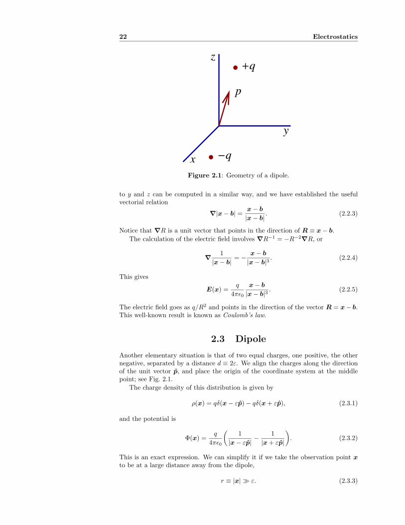
Figure 2.1: Geometry of a dipole.
to y and z can be computed in a similar way, and we have established the usefulvectorial relation
∇|x − b| =x − b
|x − b|. (2.2.3)
Notice that ∇R is a unit vector that points in the direction of R ≡ x − b.The calculation of the electric field involves ∇R−1 = −R−2∇R, or
∇1
|x − b|= −
x − b
|x − b|3. (2.2.4)
This gives
E(x) =q
4πϵ0
x − b
|x − b|3. (2.2.5)
The electric field goes as q/R2 and points in the direction of the vector R = x− b.This well-known result is known as Coulomb’s law.
2.3 Dipole
Another elementary situation is that of two equal charges, one positive, the othernegative, separated by a distance d ≡ 2ε. We align the charges along the directionof the unit vector p, and place the origin of the coordinate system at the middlepoint; see Fig. 2.1.
The charge density of this distribution is given by
ρ(x) = qδ(x − εp) − qδ(x + εp), (2.3.1)
and the potential is
Φ(x) =q
4πϵ0
"
1
|x − εp|−
1
|x + εp|
#
. (2.3.2)
This is an exact expression. We can simplify it if we take the observation point xto be at a large distance away from the dipole,
r ≡ |x| ≫ ε. (2.3.3)
2.3 Dipole 23
We can then approximate
|x ∓ εp| =0
(x ∓ εp) · (x ∓ εp)
=0
r2 ∓ 2εp · x + ε2
= r1
1 ∓ εp · x/r2 + O(ε2/r2)2
,
or1
|x ∓ εp|=
1
r
1
1 ± εp · x/r2 + O(ε2/r2)2
.
Keeping terms of order ε only, the potential becomes
Φ =1
4πϵ0
(2qεp) · xr3
.
The vector p ≡ 2qεp is the dipole moment of the charge distribution. In general,for a collection of several charges, this is defined as
p =$
A
qAxA, (2.3.4)
where xA is the position vector of the charge qA. In the present situation thedefinition implies p = (+q)(εp)+ (−q)(−εp) = 2qεp, as was stated previously. Thepotential of a dipole is then
Φ(x) =1
4πϵ0
p · xr3
, (2.3.5)
when r satisfies Eq. (2.3.3). It should be noticed that here, the potential falls off as1/r2, faster than in the case of a single point charge. This has to do with the factthat here, the charge distribution has a vanishing total charge.
It is instructive to rederive this result by directly expanding the charge densityin powers of ε. For any function f of a vector x we have f(x + εp) = f(x) + εp ·∇f(x) + O(ε2), and we can extend this result to Dirac’s distribution:
δ(x ± εp) = δ(x) ± εp · ∇δ(x) + O(ε2).
The charge density of Eq. (2.3.1) then becomes ρ(x) = −2qεp · ∇δ(x) + O(ε2), or
ρ(x) = −p · ∇δ(x). (2.3.6)
This is the charge density of a point dipole.Substituting this into Eq. (2.1.3) and setting Φ0 = 0 yields
Φ(x) = −pa
4πϵ0
!
∇′aδ(x′)
|x − x′|d3x′,
where summation over the vectorial index a is understood. The standard procedurewhen dealing with derivatives of a δ-function is to integrate by parts. The integralis then
−!
δ(x′)∇′a
1
|x − x′|d3x′ = −
!
δ(x′)(x − x′)a
|x − x′|3d3x′ = −
xa
r3,
and we have recovered Eq. (2.3.5). Notice that in these manipulations we haveinserted a result analogous to Eq. (2.2.4); the minus sign does not appear becausewe are now differentiating with respect to the primed variables.
24 Electrostatics
S
V
n
n
in
outS
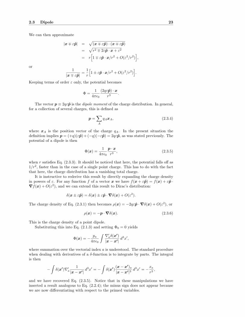
Figure 2.2: An inner boundary Sin on which Φ is specified, an outer boundarySout on which Φ is specified, and the region V in between that contains a chargedistribution ρ. The outward unit normal to both boundaries is denoted n.
From the potential of Eq. (2.3.5) we can calculate the electric field of a pointdipole. Taking a derivative with respect to x gives
∇xΦ =1
4πϵ0
3
∇x(p · x)
r3−
3(p · x)
r4∇xr
4
.
We have ∇x(p · x) = px and according to Eq. (2.2.3), ∇xr = x/r. So
∇xΦ =1
4πϵ0
3
px
r3−
3(p · x)x
r5
4
,
and a similar calculation can be carried out for the y and z components of ∇Φ.Introducing the unit vector
r = x/r = (x/r, y/r, z/r), (2.3.7)
we find that the electric field is given by
E(x) =1
4πϵ0
3(p · r)r − p
r3. (2.3.8)
This is an exact expression for the electric field of a point dipole, for which thecharge density is given by Eq. (2.3.6). For a physical dipole of finite size, thisexpression is only an approximation of the actual electric field; the approximationis good for r ≫ ε.
2.4 Boundary-value problems: Green’s theorem
[The material presented in this section is also covered in Secs. 1.8 and 1.10 ofJackson’s text.]
After the warmup exercise of the preceding two sections we are ready to facethe more serious challenge of solving boundary-value problems. A typical situationin electrostatics features a charge distribution ρ(x) between two boundaries onwhich the potential Φ(x) is specified (see Fig. 2.2) — the potential is then said tosatisfy Dirichlet boundary conditions. A concrete situation might involve an inner
2.4 Boundary-value problems: Green’s theorem 25
S
V
in
outSda
da
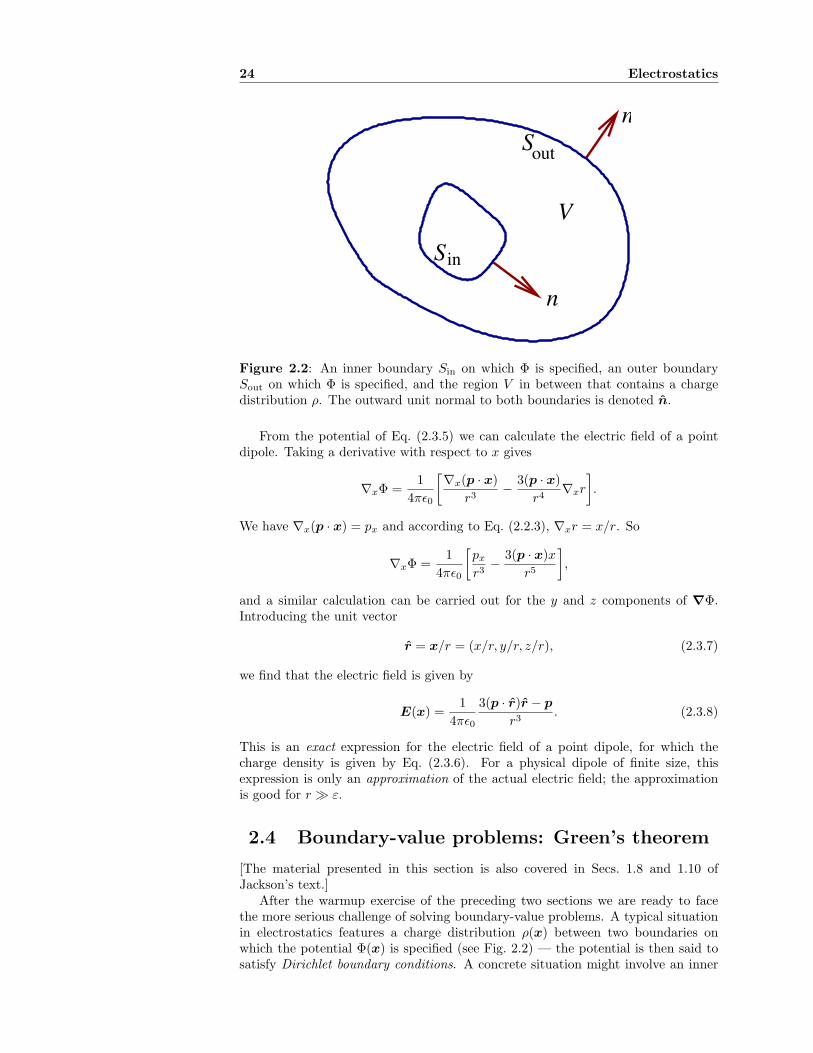
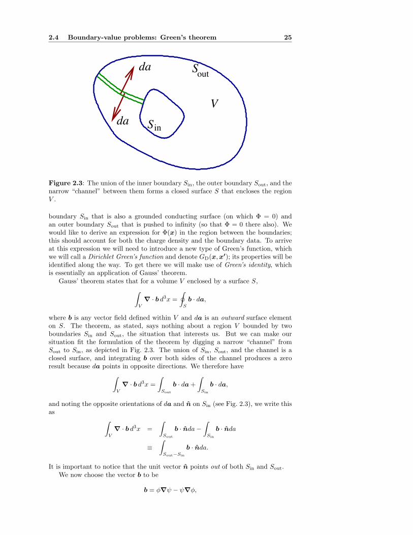
Figure 2.3: The union of the inner boundary Sin, the outer boundary Sout, and thenarrow “channel” between them forms a closed surface S that encloses the regionV .
boundary Sin that is also a grounded conducting surface (on which Φ = 0) andan outer boundary Sout that is pushed to infinity (so that Φ = 0 there also). Wewould like to derive an expression for Φ(x) in the region between the boundaries;this should account for both the charge density and the boundary data. To arriveat this expression we will need to introduce a new type of Green’s function, whichwe will call a Dirichlet Green’s function and denote GD(x,x′); its properties will beidentified along the way. To get there we will make use of Green’s identity, whichis essentially an application of Gauss’ theorem.
Gauss’ theorem states that for a volume V enclosed by a surface S,
!
V∇ · b d3x =
)
Sb · da,
where b is any vector field defined within V and da is an outward surface elementon S. The theorem, as stated, says nothing about a region V bounded by twoboundaries Sin and Sout, the situation that interests us. But we can make oursituation fit the formulation of the theorem by digging a narrow “channel” fromSout to Sin, as depicted in Fig. 2.3. The union of Sin, Sout, and the channel is aclosed surface, and integrating b over both sides of the channel produces a zeroresult because da points in opposite directions. We therefore have
!
V∇ · b d3x =
!
Sout
b · da +
!
Sin
b · da,
and noting the opposite orientations of da and n on Sin (see Fig. 2.3), we write thisas
!
V∇ · b d3x =
!
Sout
b · nda −!
Sin
b · nda
≡!
Sout−Sin
b · nda.
It is important to notice that the unit vector n points out of both Sin and Sout.We now choose the vector b to be
b = φ∇ψ − ψ∇φ,
26 Electrostatics
where φ(x) and ψ(x) are two arbitrary functions. We have ∇ · b = φ∇2ψ − ψ∇2φand Gauss’ theorem gives
!
V
%
φ∇2ψ − ψ∇2φ&
d3x =
!
Sout−Sin
%
φ∇ψ − ψ∇φ&
· nda. (2.4.1)
This is Green’s identity. For convenience we write it in the equivalent form!
V
%
φ∇′2ψ − ψ∇′2φ&
d3x′ =
!
Sout−Sin
%
φ∇′ψ − ψ∇
′φ&
· nda′,
where all fields are now expressed in terms of the new variables x′.We now pick
φ(x′) ≡ Φ(x′) ≡ scalar potential
andψ(x′) ≡ GD(x,x′) ≡ Dirichlet Green’s function,
where the properties of the “Dirichlet Green’s function” will be described in detailbelow. For now we assume that it satisfies the equation
∇′2GD(x,x′) = −4πδ(x − x′), (2.4.2)
while the scalar potential satisfies Poisson’s equation, ∇′2Φ(x′) = −ρ(x′)/ϵ0. Mak-ing these substitutions in the equation following Eq. (2.4.1) leads to
−4πΦ(x) +1
ϵ0
!
VGD(x,x′)ρ(x′) d3x′ =
!
Sout−Sin
1
Φ(x′)∇′GD(x,x′)
− GD(x,x′)∇′Φ(x′)2
· nda′,
or
Φ(x) =1
4πϵ0
!
VGD(x,x′)ρ(x′) d3x′
−1
4π
!
Sout−Sin
1
Φ(x′)∇′GD(x,x′) − GD(x,x′)∇′Φ(x′)2
· n′da′.
Apart from a remaining simplification, this is the kind of expression we were seeking.The volume integral takes care of the charge distribution within V , and the twosurface integrals take care of the boundary conditions. But there is one problem:While the value of the scalar potential is specified on the boundaries, so that thefunctions Φ(x′) are known inside the surface integrals, we are given no informationabout n · ∇′Φ(x′), its normal derivative, which also appears within the surfaceintegrals. It is not clear, therefore, how we might go about evaluating these integrals:the problem does not seem to be well posed.
To sidestep this problem we demand that the Dirichlet Green’s function satisfythe condition
GD(x,x′) = 0 when x′ is on the boundaries. (2.4.3)
Then the boundary terms involving n · ∇′Φ(x′) simply go away, because they aremultiplied by GD(x,x′) which vanishes on the boundaries. With this property wearrive at
Φ(x) =1
4πϵ0
!
VGD(x,x′)ρ(x′) d3x′
−1
4π
!
Sout−Sin
Φ(x′)n · ∇′GD(x,x′)da′. (2.4.4)
2.4 Boundary-value problems: Green’s theorem 27
This is our final expression for the scalar potential in the region V . The problemof finding this potential has been reduced to that of finding a Dirichlet Green’sfunction that satisfies Eqs. (2.4.2) and (2.4.3). Notice that this is a specialized formof our original problem: GD(x,x′) is the potential produced by a point charge ofstrength 4πϵ0 located at x, and its boundary values on Sin and Sout are zero. If wecan solve this problem and obtain the Dirichlet Green’s function, then Eq. (2.4.4)gives us the means to calculate Φ(x) in very general circumstances.
We already know that GD(x,x′) satisfies Eq. (2.4.2) and vanishes when x′ lieson Sin and Sout. We now use Green’s identity to show that the Dirichlet Green’sfunction is symmetric in its arguments:
GD(x′,x) = GD(x,x′). (2.4.5)
This implies that it is also a solution to the standard equation satisfied by a Green’sfunction,
∇2GD(x,x′) = −4πδ(x − x′), (2.4.6)
which is identical to Eq. (1.8.2). To establish Eq. (2.4.5) we take y to be theintegration variables in Green’s identity,
!
V
%
φ∇2yψ − ψ∇2
yφ&
d3y =
!
Sout−Sin
%
φ∇yψ − ψ∇yφ&
· nday,
and we pick φ(y) ≡ GD(x,y) and ψ(y) ≡ GD(x′,y). Then according to Eq. (2.4.2)we have ∇2
yφ = −4πδ(x − y) and ∇2yψ = −4πδ(x′ − y). The left-hand side of
Green’s identity gives −4π[GD(x,x′) − GD(x′,x)] after integration over d3y. Theright-hand side, on the other hand, gives zero because both φ and ψ are zero wheny is on Sin and Sout. This produces Eq. (2.4.5).
To summarize, we have found that the Dirichlet Green’s function satisfies Eq. (2.4.6),
∇2GD(x,x′) = −4πδ(x − x′),
possesses the symmetry property of Eq. (2.4.5),
GD(x′,x) = GD(x,x′),
and satisfies the boundary conditions of Eq. (2.4.3),
GD(x,x′) = 0 when x or x′ is on the boundaries.
Notice that the boundary conditions have been generalized in accordance to Eq. (2.4.5):the Dirichlet Green’s function vanishes whenever x or x′ happens to lie on theboundaries. Once the Dirichlet Green’s function has been found, the potentialproduced by a charge distribution ρ(x) in a region V between two boundaries Sin
and Sout on which Φ(x) is specified can be obtained by evaluating the integralsof Eq. (2.4.4). The task of finding a suitable Dirichlet Green’s function can onlybe completed once the boundaries Sin and Sout are fully specified; the form of theGreen’s function will depend on the shapes and locations of these boundaries. Inthe absence of boundaries, GD(x,x′) reduces to the Green’s function constructedin Sec. 1.8, G(x,x′) = |x − x′|−1.
In the following sections we will consider a restricted class of boundary-valueproblems, for which
• there is only an inner boundary Sin (Sout is pushed to infinity and does notneed to be considered);
• the inner boundary is spherical (Sin is described by the statement |x′| = R,where R is the surface’s radius);
28 Electrostatics
• the inner boundary is the surface of a grounded conductor (Φ vanishes onSin).
With these restrictions (introduced only for simplicity), Eq. (2.4.4) reduces to
Φ(x) =1
4πϵ0
!
|x′|>RGD(x,x′)ρ(x′) d3x′. (2.4.7)
In these situations, the electric field vanishes inside the conductor and there is aninduced distribution of charge on the surface. The surface charge density is givenby Eq. (1.6.9),
σ = ϵ0E · n, (2.4.8)
where E is the electric field just above Sin. This is given by E = −∇Φ(|x| = R). Toproceed we will need to find a concrete expression for the Dirichlet Green’s function.For the spherical boundary considered here, this is done by solving Eq. (2.4.6) inspherical coordinates.
2.5 Laplace’s equation in spherical coordinates
[The material presented in this section is also covered in Secs. 3.1, 3.2, and 3.5 ofJackson’s text.]
When formulated in spherical coordinates (r, θ,φ), Laplace’s equation takes theform
∇2ψ =1
r2
∂
∂r
"
r2 ∂ψ
∂r
#
+1
r2 sin θ
∂
∂θ
"
sin θ∂ψ
∂θ
#
+1
r2 sin2 θ
∂2ψ
∂φ2= 0. (2.5.1)
To solve this equation we separate the variables according to
ψ(r, θ,φ) = R(r)Y (θ,φ), (2.5.2)
and we obtain the decoupled equations
d
dr
"
r2 dR
dr
#
= ℓ(ℓ + 1)R (2.5.3)
and1
sin θ
∂
∂θ
"
sin θ∂Y
∂θ
#
+1
sin2 θ
∂2Y
∂φ2= −ℓ(ℓ + 1)Y, (2.5.4)
where ℓ(ℓ + 1) is a separation constant.The solutions to the angular equation (2.5.4) are the spherical harmonics Yℓm(θ,φ),
which are labeled by the two integers ℓ and m. While ℓ ranges from zero to infinity,m is limited to the values −ℓ,−ℓ + 1, · · · , ℓ − 1, ℓ. For m ≥ 0,
Yℓm(θ,φ) =
5
2ℓ + 1
4π
6
(ℓ − m)!
(ℓ + m)!Pm
ℓ (cos θ)eimφ, (2.5.5)
where Pmℓ (cos θ) are the associated Legendre polynomials. For m < 0 we use
Yℓm = (−1)mY ∗ℓ,−m, (2.5.6)
where an asterisk indicates complex conjugation. Particular spherical harmonicsare
Y00 =1√4π
,
2.5 Laplace’s equation in spherical coordinates 29
Y11 = −5
3
8πsin θ eiφ,
Y10 =
5
3
4πcos θ,
Y22 =1
4
5
15
2πsin2 θ e2iφ,
Y21 = −5
15
8πsin θ cos θ eiφ,
Y20 =1
2
5
5
4π(3 cos2 θ − 1).
Two fundamental properties of the spherical harmonics are that they are orthonor-mal functions, and that they form a complete set of functions of the angles θ andφ. The statement of orthonormality is
!
Y ∗ℓ′m′(θ,φ)Yℓm(θ,φ) dΩ = δℓℓ′δmm′ , (2.5.7)
where dΩ = sin θ dθdφ is an element of solid angle. The statement of completenessis that any function f(θ,φ) can be represented as a sum over spherical harmonics:
f(θ,φ) =∞$
ℓ=0
ℓ$
m=−ℓ
fℓmYℓm(θ,φ) (2.5.8)
for some coefficients fℓm. By virtue of Eq. (2.5.7), these can in fact be calculatedas
fℓm =
!
f(θ,φ)Y ∗ℓm(θ,φ) dΩ. (2.5.9)
Equation (2.5.8) means that the spherical harmonics form a complete set of basisfunctions on the sphere.
It is interesting to see what happens when Eq. (2.5.9) is substituted into Eq. (2.5.8).To avoid confusion we change the variables of integration to θ′ and φ′:
f(θ,φ) =$
ℓ
$
m
Yℓm(θ,φ)
!
f(θ′,φ′)Y ∗ℓm(θ′,φ′) dΩ′
=
!
f(θ′,φ′)
3
$
ℓ
$
m
Y ∗ℓm(θ′,φ′)Yℓm(θ,φ)
4
dΩ′.
The quantity within the large square brackets is such that when it is multipliedby f(θ′,φ′) and integrated over the primed angles, it returns f(θ,φ). This musttherefore be a product of two δ-functions, one for θ and the other for φ. Moreprecisely stated,
∞$
ℓ=0
ℓ$
m=−ℓ
Y ∗ℓm(θ′,φ′)Yℓm(θ,φ) =
δ(θ − θ′)δ(φ − φ′)
sin θ, (2.5.10)
where the factor of 1/ sin θ was inserted to compensate for the factor of sin θ′ indΩ′ (the δ-function is enforcing the condition θ′ = θ). Equation (2.5.10) is knownas the completeness relation for the spherical harmonics. This is analogous to awell-known identity,
!"
1√2π
eikx′
#∗" 1√2π
eikx
#
dk = δ(x − x′),
30 Electrostatics
in which the integral over dk replaces the discrete summation over ℓ and m; thebasis functions (2π)−1/2eikx are then analogous to the spherical harmonics.
The solutions to the radial equation (2.5.3) are power laws, R ∝ rℓ or R ∝r−(ℓ+1). The general solution is
Rℓm(r) = aℓmrℓ + bℓmr−(ℓ+1), (2.5.11)
where aℓm and bℓm are constants.The general solution to Laplace’s equation is obtained by combining Eqs. (2.5.2),
(2.5.5), (2.5.11) and summing over all possible values of ℓ and m:
ψ(r, θ,φ) =∞$
ℓ=0
ℓ$
m=−ℓ
,
aℓmrℓ + bℓmr−(ℓ+1)-
Yℓm(θ,φ). (2.5.12)
The coefficients aℓm and bℓm are determined by the boundary conditions imposedon ψ(r, θ,φ). If, for example, ψ is to be well behaved at r = 0, then bℓm ≡ 0. If, onthe other hand, ψ is to vanish at r = ∞, then aℓm ≡ 0. From these observationswe deduce that the only solution to Laplace’s equation that is well behaved at theorigin and vanishes at infinity is the trivial solution ψ = 0.
2.6 Green’s function in the absence of boundaries
[The material presented in this section is also covered in Secs. 3.6, and 3.9 of Jack-son’s text.]
Keeping in mind that our ultimate goal is to obtain the Dirichlet Green’s functionGD(x,x′) for a spherical inner boundary, in this section we attempt somethingsimpler and solve
∇2G(x,x′) = −4πδ(x − x′) (2.6.1)
in the absence of boundaries. We already know the answer: In Sec. 1.8 we foundthat
G(x,x′) =1
|x − x′|. (2.6.2)
We will obtain an alternative expression for this, one that can be generalized toaccount for the presence of spherical boundaries.
The δ-function on the right-hand side of Eq. (2.6.1) can be represented as
δ(x − x′) =δ(r − r′)
r2
δ(θ − θ′)δ(φ − φ′)
sin θ
=δ(r − r′)
r2
$
ℓm
Y ∗ℓm(θ′,φ′)Yℓm(θ,φ), (2.6.3)
where we have involved Eq. (2.5.10). The factor of 1/(r2 sin θ) was inserted be-cause in spherical coordinates, the volume element is d3x = r2 sin θ drdθdφ, and theJacobian factor of r2 sin θ must be compensated for. We then have, for example,
f(x′) =
!
f(x)δ(x − x′) d3x
=
!
f(r, θ,φ)δ(r − r′)
r2
δ(θ − θ′)δ(φ − φ′)
sin θr2 sin θ drdθdφ
=
!
f(r, θ,φ)δ(r − r′)δ(θ − θ′)δ(φ − φ′) drdθdφ
= f(r′, θ′,φ′),
2.6 Green’s function in the absence of boundaries 31
as we should.Inspired by Eq. (2.6.3) we expand the Green’s function as
G(x,x′) =$
ℓm
gℓm(r, r′)Y ∗ℓm(θ′,φ′)Yℓm(θ,φ), (2.6.4)
using the spherical harmonics Yℓm(θ,φ) for angular functions and gℓm(r, r′)Y ∗ℓm(θ′,φ′)
for radial functions. For convenience we have made the “radial function” dependon x′ through the variables r′, θ′, and φ′; these are treated as constant parameterswhen substituting G(x,x′) into Eq. (2.6.1). Applying the Laplacian operator ofEq. (2.5.1) on the Green’s function yields
∇2G(x,x′) =$
ℓm
3
1
r2
d
dr
"
r2 dgℓm
dr
#
−ℓ(ℓ + 1)
r2gℓm
4
Y ∗ℓm(θ′,φ′)Yℓm(θ,φ),
and setting this equal to −4πδ(x − x′) as expressed in Eq. (2.6.3) produces anordinary differential equation for gℓm(r, r′):
d
dr
"
r2 dgℓm
dr
#
− ℓ(ℓ + 1)gℓm = −4πδ(r − r′). (2.6.5)
This equation implies that the radial function depends only on ℓ, and not on m:gℓm(r, r′) ≡ gℓ(r, r′). To simplify the notation we will now omit the label “ℓ” onthe radial function.
To solve Eq. (2.6.5) we first observe that when r = r′, the right-hand side of theequation is zero and g is a solution to Eq. (2.5.3). We let g<(r, r′) be the solution tothe left of r′ (for r < r′) and g>(r, r′) be the solution to the right of r′ (for r > r′).We then assume that g(r, r′) can be obtained by joining the solutions at r = r′:
g(r, r′) = g<(r, r′)θ(r′ − r) + g>(r, r′)θ(r − r′), (2.6.6)
where θ(r′ − r) and θ(r − r′) are step functions. Differentiating this equation withrespect to r gives
g′(r, r′) = g′<(r, r′)θ(r′ − r) + g′>(r, r′)θ(r − r′) +'
g>(r′, r′) − g<(r′, r′)(
δ(r − r′),
where a prime on g indicates differentiation. We have involved the distributionalidentities θ′(r − r′) = δ(r − r′), θ′(r′ − r) = −δ(r − r′), and f(r)δ(r − r′) =f(r′)δ(r − r′); these were first encountered in Sec. 1.6. Multiplying by r2 yields
r2g′(r, r′) = r2g′<(r, r′)θ(r′ − r) + r2g′>(r, r′)θ(r − r′)
+ r′2'
g>(r′, r′) − g<(r′, r′)(
δ(r − r′)
and taking another derivative brings'
r2g′(r, r′)(′
='
r2g′<(r, r′)(′
θ(r′ − r) +'
r2g′>(r, r′)(′
θ(r − r′)
+ r′2'
g′>(r′, r′) − g′<(r′, r′)(
δ(r − r′)
+ r′2'
g>(r′, r′) − g<(r′, r′)(
δ′(r − r′).
Substituting this and Eq. (2.6.6) back into Eq. (2.6.5), we obtain
−4πδ(r − r′) =
3
d
dr
"
r2 dg<
dr
#
− ℓ(ℓ + 1)g<
4
θ(r′ − r)
+
3
d
dr
"
r2 dg>
dr
#
− ℓ(ℓ + 1)g>
4
θ(r − r′)
+ r′23
dg>
dr(r′, r′) −
dg<
dr(r′, r′)
4
δ(r − r′)
+ r′21
g>(r′, r′) − g<(r′, r′)2 d
drδ(r − r′).
32 Electrostatics
For the right-hand side to match the left-hand side we must demand that g<(r, r′)and g>(r, r′) be solutions to the homogeneous version of Eq. (2.6.5), as was alreadyunderstood, and that these solutions be matched according to
g>(r′, r′) − g<(r′, r′) = 0 (2.6.7)
anddg>
dr(r′, r′) −
dg<
dr(r′, r′) = −
4π
r′2. (2.6.8)
The function g(r, r′) is therefore continuous at r = r′, but its first derivative mustbe discontinuous to account for the δ-function on the right-hand side of Eq. (2.6.5).
Because g< is a solution to Eq. (2.5.3), according to Eq. (2.5.11) it must be alinear combination of terms proportional to rℓ and 1/rℓ+1. But only the first termis well behaved at r = 0, and we set
g<(r, r′) = a(r′)rℓ.
For g> we select insteadg>(r, r′) = b(r′)/rℓ+1,
which is well behaved at r = ∞. It does not matter that g< diverges at r = ∞because this function is restricted to the domain r < r′ < ∞; similarly, it does notmatter that g> diverges at r = 0 because it is restricted to the domain r > r′ > 0. Todetermine the “constants” a and b we use the matching conditions. First, Eq. (2.6.7)gives b = ar′2ℓ+1. Second, Eq. (2.6.8) gives a = 4πr′−(ℓ+1)/(2ℓ + 1). So
g<(r, r′) =4π
2ℓ + 1
rℓ
r′ℓ+1(2.6.9)
and
g>(r, r′) =4π
2ℓ + 1
r′ℓ
rℓ+1. (2.6.10)
We observe a nice symmetry between these two results. Combining Eqs. (2.6.6),(2.6.9), and (2.6.10), we find that the radial function can be expressed in the com-pact form
gℓ(r, r′) =
4π
2ℓ + 1
rℓ<
rℓ+1>
, (2.6.11)
where r< denotes the lesser of r and r′, while r> is the greater of r and r′. Thus,if r < r′ then r< = r, r> = r′, and Eq. (2.6.11) gives g(r, r′) = g<(r, r′), as itshould. Similarly, when r > r′ we have r< = r′, r> = r, and Eq. (2.6.11) givesg(r, r′) = g>(r, r′).
Substituting Eq. (2.6.11) into Eq. (2.6.4) and taking into account Eq. (2.6.2),we arrive at
1
|x − x′|=
∞$
ℓ=0
ℓ$
m=−ℓ
4π
2ℓ + 1
rℓ<
rℓ+1>
Y ∗ℓm(θ′,φ′)Yℓm(θ,φ). (2.6.12)
This very useful identity is known as the addition theorem for spherical harmonics.At first sight the usefulness of this identity might seem doubtful. After all,
we have turned something simple like an inverse distance into something horribleinvolving special functions and an infinite double sum. But we will see that when1/|x − x′| appears inside an integral, the representation of Eq. (2.6.12) can bevery useful indeed. Not relying on this identity would mean having to evaluate anintegral that involves
1
|x − x′|=
10
r2 − 2rr′[sin θ sin θ′ cos(φ − φ′) + cos θ cos θ′] + r′2,
2.6 Green’s function in the absence of boundaries 33
and such integrals typically cannot be evaluated directly: they are just too compli-cated.
Let us consider an example to illustrate the power of the addition theorem. Wewant to calculate the electrostatic potential both inside and outside a sphericaldistribution of charge with density ρ(x′) = ρ(r′). There are no boundaries in thisproblem, but the distribution is confined to a sphere of radius R. After substitutingEq. (2.6.12) into Eq. (2.1.3) and writing d3x′ = r′2dr′dΩ′, we obtain
Φ(x) =1
4πϵ0
$
ℓm
4π
2ℓ + 1Yℓm(θ,φ)
! R
0
rℓ<
rℓ+1>
ρ(r′)r′2 dr′!
Y ∗ℓm(θ′,φ′) dΩ′.
To evaluate the angular integral we multiply and divide by (4π)−1/2 ≡ Y00(θ′,φ′):
!
Y ∗ℓm(θ′,φ′) dΩ′ =
√4π
!
Y ∗ℓm(θ′,φ′)Y00(θ
′,φ′) dΩ′ =√
4πδℓ,0δm,0,
where we have involved Eq. (2.5.7). At this stage we happily realize that the infinitesum over ℓ and m involves but a single term. We therefore have
Φ(x) =1
4πϵ04π
√4πY00(θ,φ)
! R
0
r′2
r>ρ(r′) dr′ =
1
4πϵ04π
! R
0
r′2
r>ρ(r′) dr′,
and as we might have expected from the spherical symmetry of the problem, thepotential depends on r only.
To evaluate the radial integral we must be careful with the meaning of r> ≡max(r, r′). Suppose first that x is outside the charge distribution, so that r > R.Then r > r′, r> = r, and we have
4π
! R
0
r′2
r>ρ(r′) dr′ =
1
r4π
! R
0ρ(r′)r′2 dr′ =
Q
r,
where Q ≡*
ρ(x′) d3x′ = 4π* R0 ρ(r′)r′2 dr′ is the total charge of the distribution.
In this case we have
Φout(x) =1
4πϵ0
Q
r, (2.6.13)
the same result as in Eq. (2.2.2). Suppose next that x is inside the charge distri-bution, so that r < R. Then part of the integration covers the interval 0 ≤ r′ < rand the remaining part covers r ≤ r′ ≤ R. In the first part r′ is smaller than r andr> = r; in the second part r′ is larger than r and r> = r′. So
4π
! R
0
r′2
r>ρ(r′) dr′ =
1
r4π
! r
0ρ(r′)r′2 dr′ + 4π
! R
rρ(r′)r′ dr′.
In the first term we recognize
q(r) ≡!
|x′|≤rρ(x′) d3x′ = 4π
! r
0ρ(r′)r′2 dr′, (2.6.14)
the charge enclosed by a sphere of radius r; if r > R then q(r) = Q. The internalpotential can thus be expressed as
Φin(x) =1
4πϵ0
3
q(r)
r+ 4π
! R
rρ(r′)r′ dr′
4
. (2.6.15)
While the expression (2.6.15) for the internal potential depends on the detailsof the charge distribution — the particular form of the function ρ(r′) — a nicer
34 Electrostatics
conclusion applies to the electric field. The field is obtained by differentiating Φin
with respect to r, and
dΦin
dr=
1
4πϵ0
3
−q
r2+
1
r
dq
dr− 4πρr
4
.
But since dq/dr = 4πρr2 according to Eq. (2.6.14), we see that the last two termscancel out. The electric field is then
E(x) =1
4πϵ0
q(r)
r2r, (2.6.16)
both inside and outside the charge distribution; recall that when r > R, q(r) be-comes Q, the total charge. We have recovered the well-known result that for anyspherical distribution of charge, the electric field at a radius r depends only on thecharge q(r) enclosed by a sphere of that radius; and the field is the same as if allthis charge were concentrated in a point at r = 0.
2.7 Dirichlet Green’s function for a spherical
inner boundary
[The material presented in this section is also covered in Sec. 3.9 of Jackson’s text.]We now return to the task of finding the Dirichlet Green’s function GD(x,x′) for
the specific situation described near the end of Sec. 2.4, in which we have a sphericalinner boundary at |x| = R and no outer boundary. It will be a simple matter tomodify the treatment presented in Sec. 2.6 to account for the inner boundary.
As in Eq. (2.6.4), the Dirichlet Green’s function can be expanded as
GD(x,x′) =$
ℓm
gℓ(r, r′)Y ∗
ℓm(θ′,φ′)Yℓm(θ,φ). (2.7.1)
As in Eq. (2.6.6), the radial function can be expressed as
gℓ(r, r′) = g<(r, r′)θ(r′ − r) + g>(r, r′)θ(r − r′), (2.7.2)
where g< and g> are solutions to Eq. (2.5.3) that must also satisfy the matchingconditions of Eqs. (2.6.7) and (2.6.8),
g>(r′, r′) − g<(r′, r′) = 0 (2.7.3)
anddg>
dr(r′, r′) −
dg<
dr(r′, r′) = −
4π
r′2. (2.7.4)
The only difference with respect to what was done in Sec. 2.6 is that now, accordingto Eq. (2.4.3), the Green’s function must vanish on the inner boundary. This givesthe additional conditions gℓ(r = R, r′) = gℓ(r, r′ = R) = 0, or
g<(r = R, r′) = 0, g>(r, r′ = R) = 0; (2.7.5)
recall that R is now the smallest possible value of both r and r′.Since g<(r, r′) is no longer required to be well behaved at r = 0, we must set it
equal tog<(r, r′) = a(r′, R)rℓ + α(r′, R)/rℓ+1,
the general solution to Eq. (2.5.3). For g>(r, r′) we choose instead
g>(r, r′) = b(r′, R)/rℓ+1,
2.8 Point charge outside a grounded, spherical conductor 35
which is well behaved at r = ∞. Solving Eqs. (2.7.3)–(2.7.5) for the “constants”produces a = 4πr′−(ℓ+1)/(2ℓ + 1), α = −aR2ℓ+1, and b = a(r′2ℓ+1 − R2ℓ+1). Col-lecting these results gives
g<(r, r′) =4π
2ℓ + 1
1
r′ℓ+1
"
rℓ −R2ℓ+1
rℓ+1
#
(2.7.6)
and
g>(r, r′) =4π
2ℓ + 1
1
rℓ+1
"
r′ℓ −R2ℓ+1
r′ℓ+1
#
. (2.7.7)
Combining Eqs. (2.7.2), (2.7.6), and (2.7.7), we find that the radial function can beexpressed in the compact form
gℓ(r, r′) =
4π
2ℓ + 1
1
rℓ+1>
"
rℓ< −
R2ℓ+1
rℓ+1<
#
=4π
2ℓ + 1
r2ℓ+1< − R2ℓ+1
(rr′)ℓ+1, (2.7.8)
where r< denotes the lesser of r and r′, while r> is the greater of r and r′ (noticethat r<r> ≡ rr′). We see that gℓ(r, r′) vanishes on the inner boundary: Whenr = R it must be that r < r′, so that r< = r = R, and the terms within thebrackets vanish; on the other hand, when r′ = R it must be that r′ < r, so thatr< = r′ = R, and the same conclusion applies.
The Dirichlet Green’s function is obtained by substituting Eq. (2.7.8) into Eq. (2.7.1):
GD(x,x′) =$
ℓm
4π
2ℓ + 1
1
rℓ+1>
"
rℓ< −
R2ℓ+1
rℓ+1<
#
Y ∗ℓm(θ′,φ′)Yℓm(θ,φ). (2.7.9)
This is slightly more complicated than Eq. (2.6.12), but still manageable. Noticethat the Dirichlet Green’s function reduces to 1/|x − x′| when R = 0. It would bestraightforward to generalize this derivation to account also for the presence of anouter boundary; we shall not pursue this here.
2.8 Point charge outside a grounded, spherical
conductor
[The material presented in this section is also covered in Sec. 2.2 of Jackson’s text.]The electrostatic potential outside a grounded, spherical conductor of radius R
is given by Eq. (2.4.7),
Φ(x) =1
4πϵ0
!
|x′|>RGD(x,x′)ρ(x′) d3x′, (2.8.1)
and the Dirichlet Green’s function was obtained as
GD(x,x′) =$
ℓm
4π
2ℓ + 1
1
rℓ+1>
"
rℓ< −
R2ℓ+1
rℓ+1<
#
Y ∗ℓm(θ′,φ′)Yℓm(θ,φ) (2.8.2)
in the preceding section. The charge density induced on the surface of the conductoris given by Eq. (2.4.8), σ = ϵ0E · n, where E is the electric field just above theconductor and n ≡ r is the surface’s unit normal. Because E = −∇Φ, this worksout to be
σ = −ϵ0∂Φ
∂r
+
+
+
+
r=R
. (2.8.3)
We place a point charge q on the z axis, at a distance z0 > R from the centre ofthe conducting sphere. The charge’s position vector is z0 = z0z and its sphericalcoordinates are r0 = z0, θ0 = 0, and φ0 is undetermined. The charge density is
ρ(x′) = qδ(x′ − z0). (2.8.4)
36 Electrostatics
Substituting this into Eq. (2.8.1) gives
Φ(x) =q
4πϵ0GD(x,z0)
=q
4πϵ0
$
ℓm
4π
2ℓ + 1
"
rℓ<
rℓ+1>
−R2ℓ+1
rℓ+1< rℓ+1
>
#
Y ∗ℓm(0,φ0)Yℓm(θ,φ),
where r< now stands for the lesser of r and z0, while r> stands for the greater ofthe two. It is a property of the spherical harmonics that
Yℓm(0,φ0) =
5
2ℓ + 1
4πδm,0,
so that the potential is actually independent of φ0 and involves a single sum overℓ. It is another property of the spherical harmonics that for m = 0, they reduce toordinary Legendre polynomials,
Yℓ,0(θ,φ) =
5
2ℓ + 1
4πPℓ(cos θ).
After cleaning up the algebra, the final expression for the potential is
Φ(x) =q
4πϵ0
∞$
ℓ=0
"
rℓ<
rℓ+1>
−R2ℓ+1/zℓ+1
0
rℓ+1
#
Pℓ(cos θ). (2.8.5)
We see that the potential depends on r and θ only; the fact that it does not dependon φ reflects the axial symmetry of the problem.
Before moving on we pause and recall the main properties of the Legendrepolynomials. These are ordinary polynomials of order ℓ; if ℓ is even the functionPℓ(x) contains only even terms, while if ℓ is odd it contains only odd terms. Forexample,
P0(x) = 1,
P1(x) = x,
P2(x) =1
2(3x2 − 1),
P3(x) =1
2(5x3 − 3x),
P4(x) =1
8(35x4 − 30x2 + 3).
The Legendre polynomials are orthogonal functions,
! 1
−1Pℓ′(x)Pℓ(x) dx =
2
2ℓ + 1δℓ′ℓ, (2.8.6)
and they possess the special values
P2n(0) = (−1)n (2n − 1)!!
(2n)!!, P2n+1(0) = 0, Pℓ(1) = 1, (2.8.7)
where the double factorial notation means (2n)!! = (2n)(2n − 2)(2n − 4) · · · (2) or(2n − 1)!! = (2n − 1)(2n − 3)(2n − 5) · · · (1).
The potential of Eq. (2.8.5) is expressed as an infinite sum over ℓ. We willevaluate this sum in a moment, but for now we calculate the charge density σ(θ)
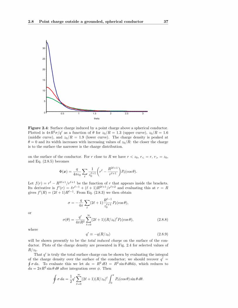
2.8 Point charge outside a grounded, spherical conductor 37
0
5
10
15
20
25
30
0.5 1 1.5 2 2.5 3
theta
Figure 2.4: Surface charge induced by a point charge above a spherical conductor.Plotted is 4πR2σ/q′ as a function of θ for z0/R = 1.3 (upper curve), z0/R = 1.6(middle curve), and z0/R = 1.9 (lower curve). The charge density is peaked atθ = 0 and its width increases with increasing values of z0/R: the closer the chargeis to the surface the narrower is the charge distribution.
on the surface of the conductor. For r close to R we have r < z0, r< = r, r> = z0,and Eq. (2.8.5) becomes
Φ(x) =q
4πϵ0
$
ℓ
1
zℓ+10
"
rℓ −R2ℓ+1
rℓ+1
#
Pℓ(cos θ).
Let f(r) = rℓ − R2ℓ+1/rℓ+1 be the function of r that appears inside the brackets.Its derivative is f ′(r) = ℓrℓ−1 + (ℓ + 1)R2ℓ+1/rℓ+2 and evaluating this at r = Rgives f ′(R) = (2ℓ + 1)Rℓ−1. From Eq. (2.8.3) we then obtain
σ = −q
4π
$
ℓ
(2ℓ + 1)Rℓ−1
zℓ+10
Pℓ(cos θ),
or
σ(θ) =q′
4πR2
∞$
ℓ=0
(2ℓ + 1)(R/z0)ℓPℓ(cos θ), (2.8.8)
whereq′ ≡ −q(R/z0) (2.8.9)
will be shown presently to be the total induced charge on the surface of the con-ductor. Plots of the charge density are presented in Fig. 2.4 for selected values ofR/z0.
That q′ is truly the total surface charge can be shown by evaluating the integralof the charge density over the surface of the conductor; we should recover q′ =7
σ da. To evaluate this we let da = R2 dΩ = R2 sin θ dθdφ, which reduces toda = 2πR2 sin θ dθ after integration over φ. Then
)
σ da =1
2q′
∞$
ℓ=0
(2ℓ + 1)(R/z0)ℓ
! π
0Pℓ(cos θ) sin θ dθ.
38 Electrostatics
The integral over θ is equal to* 1−1 Pℓ(x)P0(x) dx = 2δℓ,0 by virtue of Eq. (2.8.6),
and we obtain7
σ da = q′, as required.The potential of Eq. (2.8.5) can be decomposed as
Φ(x) = Φq(x) + Φq′(x), (2.8.10)
where
Φq(x) =q
4πϵ0
∞$
ℓ=0
rℓ<
rℓ+1>
Pℓ(cos θ) (2.8.11)
is the potential that would be obtained in the absence of a boundary, and
Φq′(x) =q′
4πϵ0
∞$
ℓ=0
(z′0)ℓ
rℓ+1Pℓ(cos θ) (2.8.12)
is the modification introduced by the boundary condition Φ(r = R) = 0; hereq′ = −q(R/z0) was defined in Eq. (2.8.9) and
z′0 ≡ R2/z0. (2.8.13)
Notice that z′0/R = R/z0 < 1, so that z′0 < R ≤ r.The sums over ℓ can now be evaluated. For Φq we already know that Eq. (2.8.11)
is equivalent to
Φq(x) =1
4πϵ0
q
|x − z0|, (2.8.14)
because Φq is the potential produced by a charge q at a position z0 = z0z in theabsence of boundaries. By analogy, because z′0 < r we have that Eq. (2.8.12) isequivalent to
Φq′(x) =1
4πϵ0
q′
|x − z′
0|, (2.8.15)
where z′
0 = z′0z. This is the potential of a fictitious image charge q′ at a position z′
0
inside the conductor. While in reality the charge q′ is distributed on the surface ofthe conductor, the potential Φq′ is the same as if all this charge were concentratedat z′
0.This observation is the basis for the method of images, which consists of finding
solutions for the potential in the presence of conducting surfaces by guessing thecorrect positions of the correct number of image charges. It is a powerful, but tricky,method.
2.9 Ring of charge outside a grounded, spherical
conductor
In this section we consider a uniformly charged ring of radius a > R. If the ring isplaced in the x-y plane, its charge density is described by
ρ(x′) =q
2πa2δ(r′ − a)δ(θ′ − π
2 ), (2.9.1)
where q =*
ρ(x′) d3x′ is the ring’s total charge. The δ-function in r′ indicates thatthe ring is infinitely thin, while the δ-function in θ′ tells us that it is placed in thex-y plane, as was previously stated.
Substituting Eq. (2.9.1) into Eq. (2.8.1) along with Eq. (2.8.2) gives
Φ(x) =1
4πϵ0
q
2πa2
$
ℓm
4π
2ℓ + 1Yℓm(θ,φ)
! ∞
0
"
rℓ<
rℓ+1>
−R2ℓ+1
rℓ+1< rℓ+1
>
#
δ(r′ − a)r′2 dr′
×!
Y ∗ℓm(θ′,φ′)δ(θ′ − π
2 ) dΩ′,
2.9 Ring of charge outside a grounded, spherical conductor 39
where dΩ′ = sin θ′ dθ′dφ, r< = min(r, r′), and r> = max(r, r′). To perform the φ′
integration we recall that Y ∗ℓm ∝ e−imφ′
, so that integrating gives zero unless m = 0.So
! 2π
0Y ∗
ℓm(θ′,φ′) dφ′ = 2πYℓ,0(θ′)δm,0.
Integration over θ′ then gives
2πYℓ,0(π2 )δm,0 = 2π
5
2ℓ + 1
4πPℓ(0)δm,0.
On the other hand, the radial integration gives
a2
"
rℓ<
rℓ+1>
−R2ℓ+1
rℓ+1< rℓ+1
>
#
where r< now stands for the lesser of r and a, while r> stands for the greater ofthe two. With these results the potential becomes
Φ(x) =q
4πϵ0
$
ℓ
4π
2ℓ + 1Yℓ,0(θ)
"
rℓ<
rℓ+1>
−R2ℓ+1
rℓ+1< rℓ+1
>
#
5
2ℓ + 1
4πPℓ(0).
Invoking once more the relation between Yℓ,0(θ) and Pℓ(cos θ), we arrive at
Φ(x) =q
4πϵ0
∞$
ℓ=0
Pℓ(0)
"
rℓ<
rℓ+1>
−R2ℓ+1/aℓ+1
rℓ+1
#
Pℓ(cos θ). (2.9.2)
Once more the potential is independent of φ, and is expressed as an infinite sumover ℓ. Once again we will see that the sum over ℓ can be evaluated.
We first calculate the charge density on the surface of the conductor. For r closeto R and therefore smaller than a, we have r< = r, r> = a, and Eq. (2.9.2) becomes
Φ(x) =q
4πϵ0
∞$
ℓ=0
Pℓ(0)f(r)
aℓ+1Pℓ(cos θ),
where the function f(r) = rℓ − R2ℓ+1/rℓ+1 was previously encountered in Sec. 2.8.We recall that f ′(R) = (2ℓ + 1)Rℓ−1, and Eq. (2.8.3) gives
σ = −q
4π
$
ℓ
(2ℓ + 1)Pℓ(0)Rℓ−1
aℓ+1Pℓ(cos θ),
or
σ(θ) =q′
4πR2
∞$
ℓ=0
(2ℓ + 1)Pℓ(0)(R/a)ℓPℓ(cos θ), (2.9.3)
whereq′ ≡ −q(R/a) (2.9.4)
is the total charge on the conducting surface. Plots of the surface charge densityare presented in Fig. 2.5 for selected values of R/a.
As in the previous section the potential of Eq. (2.9.2) can be decomposed as
Φ(x) = Φq(x) + Φq′(x), (2.9.5)
where Φq is the potential of a ring of total charge q and radius a, while Φq′ is thepotential of a fictitious image ring of total charge q′ and radius a′ = R2/a. (Youshould work through the details and make sure that these statements are true.)
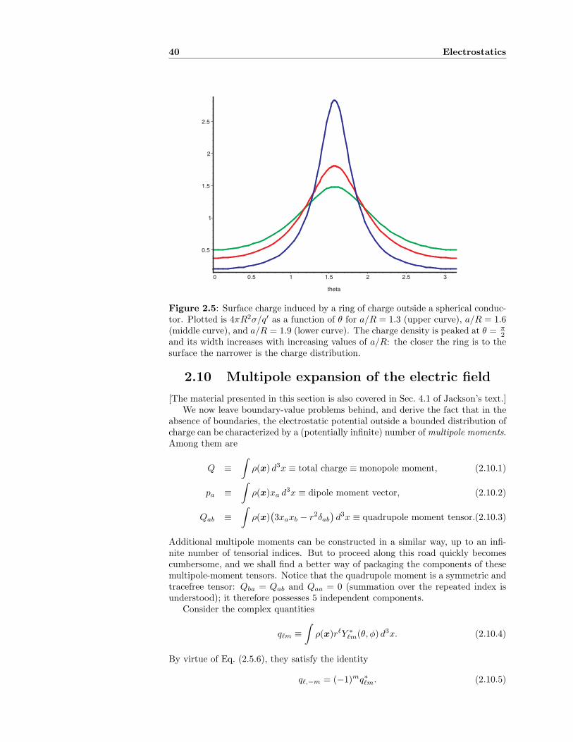
40 Electrostatics
0.5
1
1.5
2
2.5
0 0.5 1 1.5 2 2.5 3
theta
Figure 2.5: Surface charge induced by a ring of charge outside a spherical conduc-tor. Plotted is 4πR2σ/q′ as a function of θ for a/R = 1.3 (upper curve), a/R = 1.6(middle curve), and a/R = 1.9 (lower curve). The charge density is peaked at θ = π
2and its width increases with increasing values of a/R: the closer the ring is to thesurface the narrower is the charge distribution.
2.10 Multipole expansion of the electric field
[The material presented in this section is also covered in Sec. 4.1 of Jackson’s text.]We now leave boundary-value problems behind, and derive the fact that in the
absence of boundaries, the electrostatic potential outside a bounded distribution ofcharge can be characterized by a (potentially infinite) number of multipole moments.Among them are
Q ≡!
ρ(x) d3x ≡ total charge ≡ monopole moment, (2.10.1)
pa ≡!
ρ(x)xa d3x ≡ dipole moment vector, (2.10.2)
Qab ≡!
ρ(x)%
3xaxb − r2δab
&
d3x ≡ quadrupole moment tensor.(2.10.3)
Additional multipole moments can be constructed in a similar way, up to an infi-nite number of tensorial indices. But to proceed along this road quickly becomescumbersome, and we shall find a better way of packaging the components of thesemultipole-moment tensors. Notice that the quadrupole moment is a symmetric andtracefree tensor: Qba = Qab and Qaa = 0 (summation over the repeated index isunderstood); it therefore possesses 5 independent components.
Consider the complex quantities
qℓm ≡!
ρ(x)rℓY ∗ℓm(θ,φ) d3x. (2.10.4)
By virtue of Eq. (2.5.6), they satisfy the identity
qℓ,−m = (−1)mq∗ℓm. (2.10.5)
2.10 Multipole expansion of the electric field 41
Because m ranges from −ℓ to ℓ, for a given ℓ there are 2ℓ + 1 independent realquantities within the qℓms. For ℓ = 0 we have only one, and we will see that q00 isproportional to the total charge. For ℓ = 1 we have three independent quantities,and we will see that the q1ms give the components of the dipole moment vector. Forℓ = 2 we have five independent quantities, and we will see that the q2ms give thecomponents of the quadrupole moment tensor. Thus, the quantities of Eq. (2.10.4)give a convenient packaging of the multipole moments, to all orders.
To evaluate Eq. (2.10.4) for ℓ = 0 we recall that Y ∗00 = (4π)−1/2, so that
q00 =1√4π
Q. (2.10.6)
We see that indeed, q00 is directly related to the total charge. For ℓ = 1 we haverY ∗
11 = −(3/8π)1/2(r sin θ)e−iφ = −(3/8π)1/2(x− iy) and rY ∗10 = (3/4π)1/2r cos θ =
(3/4π)1/2z. This gives
q11 = −5
3
8π
%
px − ipy
&
, q10 =
5
3
4πpz, (2.10.7)
and we see that indeed, the q1ms are directly related to the dipole moment vec-tor. For ℓ = 2 we have r2Y ∗
22 = (15/32π)1/2(r sin θe−iφ)2 = (15/32π)1/2(x − iy)2,r2Y ∗
21 = −(15/8π)1/2(r sin θe−iφ)(r cos θ) = −(15/8π)1/2(x − iy)z, and r2Y ∗20 =
(5/16π)1/2r2(3 cos2 θ − 1) = (5/16π)1/2(3z2 − r2). This gives
q22 =1
12
5
15
2π
%
Qxx − Qyy − 2iQxy
&
,
q21 = −1
6
5
15
2π
%
Qxz − iQyz
&
,
q20 =1
2
5
5
4πQzz, (2.10.8)
and we see that indeed, the q2ms are directly related to the quadrupole momenttensor. For higher values of ℓ it is best to stick with the definition of Eq. (2.10.4).
How are the multipole moments qℓm related to the potential? The answer comesfrom Eq. (2.1.3) in which we set Φ0(x) = 0 (because we are no longer consideringboundaries) and substitute Eq. (2.6.12):
Φ(x) =1
4πϵ0
$
ℓm
4π
2ℓ + 1Yℓm(θ,φ)
!
ρ(x′)rℓ<
rℓ+1>
Y ∗ℓm(θ′,φ′) d3x′.
Because we are looking at the potential outside the charge distribution, r is largerthan r′ and we can set r< = r′, r> = r. This gives
Φ(x) =1
4πϵ0
$
ℓm
4π
2ℓ + 1
Yℓm(θ,φ)
rℓ+1
!
ρ(x′)r′ℓY ∗ℓm(θ′,φ′) d3x′.
We recognize the integral over the primed variables as the definition of the qℓms,and we arrive at
Φ(r, θ,φ) =1
4πϵ0
∞$
ℓ=0
ℓ$
m=−ℓ
4π
2ℓ + 1qℓm
Yℓm(θ,φ)
rℓ+1. (2.10.9)
This is an expansion of the potential in inverse powers of r, and the multipolemoments play the role of expansion coefficients.
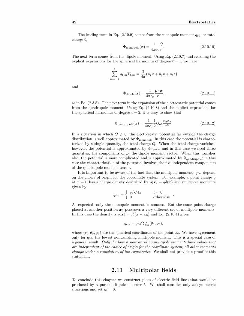
42 Electrostatics
The leading term in Eq. (2.10.9) comes from the monopole moment q00, or totalcharge Q:
Φmonopole(x) =1
4πϵ0
Q
r. (2.10.10)
The next term comes from the dipole moment. Using Eq. (2.10.7) and recalling theexplicit expressions for the spherical harmonics of degree ℓ = 1, we have
1$
m=−1
q1,mY1,m =3
4π
%
pxx + pyy + pzz&
and
Φdipole(x) =1
4πϵ0
p · xr3
, (2.10.11)
as in Eq. (2.3.5). The next term in the expansion of the electrostatic potential comesfrom the quadrupole moment. Using Eq. (2.10.8) and the explicit expressions forthe spherical harmonics of degree ℓ = 2, it is easy to show that
Φquadrupole(x) =1
4πϵ0
1
2Qab
xaxb
r5. (2.10.12)
In a situation in which Q = 0, the electrostatic potential far outside the chargedistribution is well approximated by Φmonopole; in this case the potential is charac-terized by a single quantity, the total charge Q. When the total charge vanishes,however, the potential is approximated by Φdipole, and in this case we need threequantities, the components of p, the dipole moment vector. When this vanishesalso, the potential is more complicated and is approximated by Φquadrupole; in thiscase the characterization of the potential involves the five independent componentsof the quadrupole moment tensor.
It is important to be aware of the fact that the multipole moments qℓm dependon the choice of origin for the coordinate system. For example, a point charge qat x = 0 has a charge density described by ρ(x) = qδ(x) and multipole momentsgiven by
qℓm =
8
q/√
4π ℓ = 00 otherwise
.
As expected, only the monopole moment is nonzero. But the same point chargeplaced at another position x0 possesses a very different set of multipole moments.In this case the density is ρ(x) = qδ(x − x0) and Eq. (2.10.4) gives
qℓm = qr0ℓY ∗
ℓm(θ0,φ0),
where (r0, θ0,φ0) are the spherical coordinates of the point x0. We have agreementonly for q00, the lowest nonvanishing multipole moment. This is a special case ofa general result: Only the lowest nonvanishing multipole moments have values thatare independent of the choice of origin for the coordinate system; all other momentschange under a translation of the coordinates. We shall not provide a proof of thisstatement.
2.11 Multipolar fields
To conclude this chapter we construct plots of electric field lines that would beproduced by a pure multipole of order ℓ. We shall consider only axisymmetricsituations and set m = 0.
2.11 Multipolar fields 43
The potential for such a multipole is obtained from Eq. (2.10.9), in which weset [4π/(2ℓ + 1)]qℓ0Yℓ0(θ,φ) = qℓPℓ(cos θ). This gives
Φ(r, θ) =qℓ
4πϵ0
Pℓ(cos θ)
rℓ+1, (2.11.1)
and the corresponding electric field is
E(r, θ) =qℓ
4πϵ0
1
rℓ+2
1
(ℓ + 1)Pℓ(cos θ)r + sin θP ′ℓ(cos θ)θ
2
, (2.11.2)
in which a prime indicates differentiation with respect to the argument.
The electric field lines are represented by parametric curves x(λ) for which λ isan arbitrary parameter. These curves are integral curves of the vector field E(x),which means that the tangent vector to the curves is defined to be everywhere equalto E. Thus, the field lines are determined by solving the differential equations
dx
dλ= E(x). (2.11.3)
In the case of an axisymmetric field the curves can depend on r and θ only, and wehave
dx
dλ=
∂x
∂r
dr
dλ+
∂x
∂θ
dθ
dλ=
dr
dλr + r
dθ
dλθ.
This shows that dr/dλ = Er and rdθ/dλ = Eθ, and using Eq. (2.11.2) producesdr ∝ (ℓ + 1)Pℓ and rdθ ∝ sin θP ′
ℓ , or
dr
r=
(ℓ + 1)Pℓ(cos θ)
sin θP ′ℓ(cos θ)
dθ = −(ℓ + 1)Pℓ(µ)
(1 − µ2)P ′ℓ(µ)
dµ, (2.11.4)
where µ = cos θ. The field lines are therefore determined by integrating Eq. (2.11.4).
To accomplish this it is useful to recall the differential equation satisfied by theLegendre polynomials,
d
dµ(1 − µ2)
dPℓ
dµ+ ℓ(ℓ + 1)Pℓ = 0.
We solve this algebraically for Pℓ and substitute into Eq. (2.11.4) to get
ℓdr
r=
'
(1 − µ2)P ′ℓ
(′
(1 − µ2)P ′ℓ(µ)
dµ.
This can be integrated at once, and we obtain
ℓ ln r = ln'
(1 − µ2)P ′ℓ
(
+ constant,
or
r(θ) = r0
+
+sin2 θP ′ℓ(cos θ)
+
+
1/ℓ, (2.11.5)
where r0 is constant on each curve, but varies from one curve to the next. Equation(2.11.5) gives the mathematical description of the electric field lines of an axisym-metric multipole of degree ℓ. The field lines are plotted for selected values of ℓ inFig. 2.6.
44
Electro
statics
–2
–1
1
2
–4 –2 2 4
–3
–2
–1
1
2
3
–4 –2 2 4
–4
–2
0
2
4
–4 –2 2 4
–4
–2
2
4
–4 –2 2 4
–4
–2
2
4
–4 –2 2 4
–4
–2
2
4
–4 –2 2 4
Fig
ure
2.6
:E
lectricfield
lines
ofan
axisymm
etricm
ultip
ole,for
selectedvalu
esof
the
multip
oleord
erℓ.
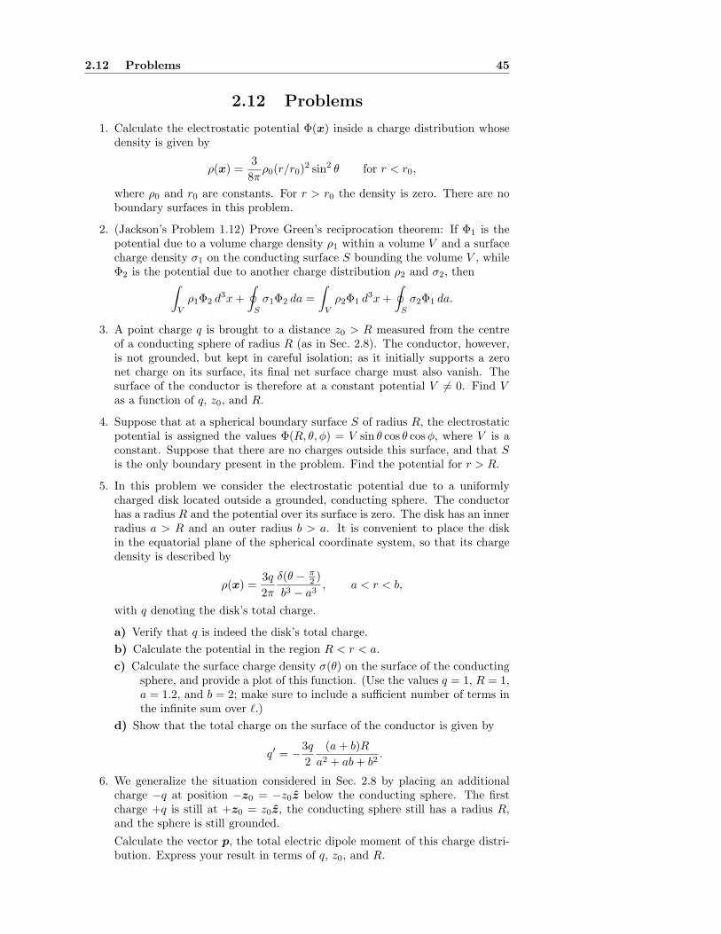
2.12 Problems 45
2.12 Problems
1. Calculate the electrostatic potential Φ(x) inside a charge distribution whosedensity is given by
ρ(x) =3
8πρ0(r/r0)
2 sin2 θ for r < r0,
where ρ0 and r0 are constants. For r > r0 the density is zero. There are noboundary surfaces in this problem.
2. (Jackson’s Problem 1.12) Prove Green’s reciprocation theorem: If Φ1 is thepotential due to a volume charge density ρ1 within a volume V and a surfacecharge density σ1 on the conducting surface S bounding the volume V , whileΦ2 is the potential due to another charge distribution ρ2 and σ2, then
!
Vρ1Φ2 d3x +
)
Sσ1Φ2 da =
!
Vρ2Φ1 d3x +
)
Sσ2Φ1 da.
3. A point charge q is brought to a distance z0 > R measured from the centreof a conducting sphere of radius R (as in Sec. 2.8). The conductor, however,is not grounded, but kept in careful isolation; as it initially supports a zeronet charge on its surface, its final net surface charge must also vanish. Thesurface of the conductor is therefore at a constant potential V = 0. Find Vas a function of q, z0, and R.
4. Suppose that at a spherical boundary surface S of radius R, the electrostaticpotential is assigned the values Φ(R, θ,φ) = V sin θ cos θ cos φ, where V is aconstant. Suppose that there are no charges outside this surface, and that Sis the only boundary present in the problem. Find the potential for r > R.
5. In this problem we consider the electrostatic potential due to a uniformlycharged disk located outside a grounded, conducting sphere. The conductorhas a radius R and the potential over its surface is zero. The disk has an innerradius a > R and an outer radius b > a. It is convenient to place the diskin the equatorial plane of the spherical coordinate system, so that its chargedensity is described by
ρ(x) =3q
2π
δ(θ − π2 )
b3 − a3, a < r < b,
with q denoting the disk’s total charge.
a) Verify that q is indeed the disk’s total charge.
b) Calculate the potential in the region R < r < a.
c) Calculate the surface charge density σ(θ) on the surface of the conductingsphere, and provide a plot of this function. (Use the values q = 1, R = 1,a = 1.2, and b = 2; make sure to include a sufficient number of terms inthe infinite sum over ℓ.)
d) Show that the total charge on the surface of the conductor is given by
q′ = −3q
2
(a + b)R
a2 + ab + b2.
6. We generalize the situation considered in Sec. 2.8 by placing an additionalcharge −q at position −z0 = −z0z below the conducting sphere. The firstcharge +q is still at +z0 = z0z, the conducting sphere still has a radius R,and the sphere is still grounded.
Calculate the vector p, the total electric dipole moment of this charge distri-bution. Express your result in terms of q, z0, and R.
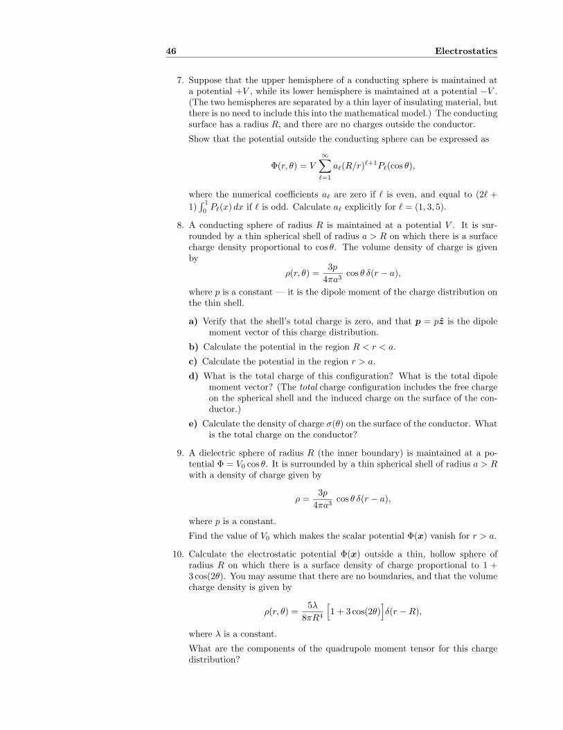
46 Electrostatics
7. Suppose that the upper hemisphere of a conducting sphere is maintained ata potential +V , while its lower hemisphere is maintained at a potential −V .(The two hemispheres are separated by a thin layer of insulating material, butthere is no need to include this into the mathematical model.) The conductingsurface has a radius R, and there are no charges outside the conductor.
Show that the potential outside the conducting sphere can be expressed as
Φ(r, θ) = V∞$
ℓ=1
aℓ(R/r)ℓ+1Pℓ(cos θ),
where the numerical coefficients aℓ are zero if ℓ is even, and equal to (2ℓ +
1)* 10 Pℓ(x) dx if ℓ is odd. Calculate aℓ explicitly for ℓ = (1, 3, 5).
8. A conducting sphere of radius R is maintained at a potential V . It is sur-rounded by a thin spherical shell of radius a > R on which there is a surfacecharge density proportional to cos θ. The volume density of charge is givenby
ρ(r, θ) =3p
4πa3cos θ δ(r − a),
where p is a constant — it is the dipole moment of the charge distribution onthe thin shell.
a) Verify that the shell’s total charge is zero, and that p = pz is the dipolemoment vector of this charge distribution.
b) Calculate the potential in the region R < r < a.
c) Calculate the potential in the region r > a.
d) What is the total charge of this configuration? What is the total dipolemoment vector? (The total charge configuration includes the free chargeon the spherical shell and the induced charge on the surface of the con-ductor.)
e) Calculate the density of charge σ(θ) on the surface of the conductor. Whatis the total charge on the conductor?
9. A dielectric sphere of radius R (the inner boundary) is maintained at a po-tential Φ = V0 cos θ. It is surrounded by a thin spherical shell of radius a > Rwith a density of charge given by
ρ =3p
4πa3cos θ δ(r − a),
where p is a constant.
Find the value of V0 which makes the scalar potential Φ(x) vanish for r > a.
10. Calculate the electrostatic potential Φ(x) outside a thin, hollow sphere ofradius R on which there is a surface density of charge proportional to 1 +3 cos(2θ). You may assume that there are no boundaries, and that the volumecharge density is given by
ρ(r, θ) =5λ
8πR4
1
1 + 3 cos(2θ)2
δ(r − R),
where λ is a constant.
What are the components of the quadrupole moment tensor for this chargedistribution?
Chapter 3
Magnetostatics
3.1 Equations of magnetostatics
For time-independent situations, the part of Maxwell’s equations that involve themagnetic field are decoupled from those involving the electric field, and they can bedealt with separately. The equations of magnetostatics are Poisson’s equation forthe vector potential,
∇2A(x) = −µ0j(x), (3.1.1)
the Lorenz (or Coulomb) gauge condition
∇ · A = 0, (3.1.2)
and the relation between potential and field,
B = ∇ × A. (3.1.3)
We recall that the current density must satisfy the statement of charge conservation,∇ · j = 0.
Because Eq. (3.1.1) is very similar to the electrostatic equation (2.1.1), the toolsintroduced in Chapter 2 to solve Poisson’s equation can be taken over directly tomagnetostatics. And because we already have gained much experience solving suchequations, it will suffice to keep our discussion of magnetostatics quite brief. Inparticular, it will be sufficient to solve Eq. (3.1.1) in the absence of boundaries. Wetherefore write the solution as
A(x) =µ0
4π
!
j(x′)
|x − x′|d3x′, (3.1.4)
recalling the results of Sec. 1.8.
3.2 Circular current loop
[The material presented in this section is also covered in Sec. 5.5 of Jackson’s text.]As our first application we calculate the magnetic field produced by a current I
flowing inside a circular loop of radius R. We place the loop in the x-y plane, atz = 0. To evaluate the integral of Eq. (3.1.4) for this situation we will use sphericalcoordinates and express the Green’s function as in Eq. (2.6.12),
1
|x − x′|=
∞$
ℓ=0
ℓ$
m=−ℓ
4π
2ℓ + 1
rℓ<
rℓ+1>
Y ∗ℓm(θ′,φ′)Yℓm(θ,φ), (3.2.1)
where r< is the lesser of r and r′, while r> is the greater of the two.
47
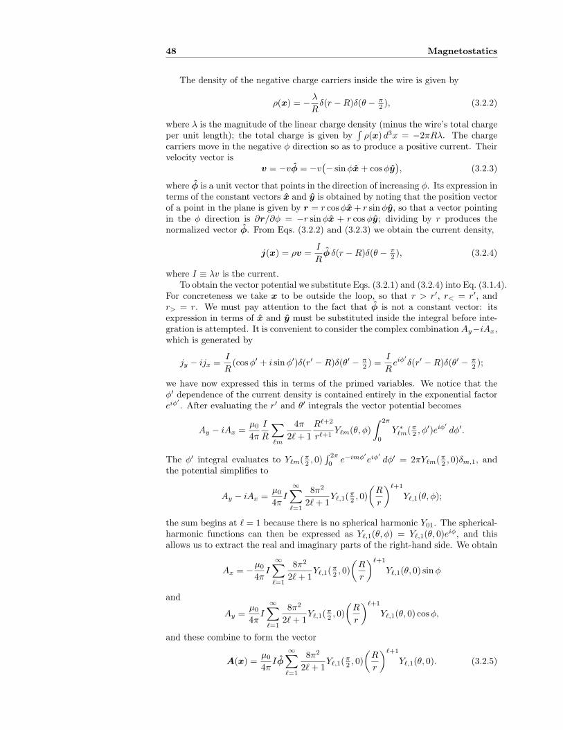
48 Magnetostatics
The density of the negative charge carriers inside the wire is given by
ρ(x) = −λ
Rδ(r − R)δ(θ − π
2 ), (3.2.2)
where λ is the magnitude of the linear charge density (minus the wire’s total chargeper unit length); the total charge is given by
*
ρ(x) d3x = −2πRλ. The chargecarriers move in the negative φ direction so as to produce a positive current. Theirvelocity vector is
v = −vφ = −v%
− sin φx + cos φy&
, (3.2.3)
where φ is a unit vector that points in the direction of increasing φ. Its expression interms of the constant vectors x and y is obtained by noting that the position vectorof a point in the plane is given by r = r cos φx + r sinφy, so that a vector pointingin the φ direction is ∂r/∂φ = −r sin φx + r cos φy; dividing by r produces thenormalized vector φ. From Eqs. (3.2.2) and (3.2.3) we obtain the current density,
j(x) = ρv =I
Rφ δ(r − R)δ(θ − π
2 ), (3.2.4)
where I ≡ λv is the current.To obtain the vector potential we substitute Eqs. (3.2.1) and (3.2.4) into Eq. (3.1.4).
For concreteness we take x to be outside the loop, so that r > r′, r< = r′, andr> = r. We must pay attention to the fact that φ is not a constant vector: itsexpression in terms of x and y must be substituted inside the integral before inte-gration is attempted. It is convenient to consider the complex combination Ay−iAx,which is generated by
jy − ijx =I
R(cos φ′ + i sin φ′)δ(r′ − R)δ(θ′ − π
2 ) =I
Reiφ′
δ(r′ − R)δ(θ′ − π2 );
we have now expressed this in terms of the primed variables. We notice that theφ′ dependence of the current density is contained entirely in the exponential factoreiφ′
. After evaluating the r′ and θ′ integrals the vector potential becomes
Ay − iAx =µ0
4π
I
R
$
ℓm
4π
2ℓ + 1
Rℓ+2
rℓ+1Yℓm(θ,φ)
! 2π
0Y ∗
ℓm(π2 ,φ′)eiφ′
dφ′.
The φ′ integral evaluates to Yℓm(π2 , 0)
* 2π0 e−imφ′
eiφ′
dφ′ = 2πYℓm(π2 , 0)δm,1, and
the potential simplifies to
Ay − iAx =µ0
4πI
∞$
ℓ=1
8π2
2ℓ + 1Yℓ,1(
π2 , 0)
"
R
r
#ℓ+1
Yℓ,1(θ,φ);
the sum begins at ℓ = 1 because there is no spherical harmonic Y01. The spherical-harmonic functions can then be expressed as Yℓ,1(θ,φ) = Yℓ,1(θ, 0)eiφ, and thisallows us to extract the real and imaginary parts of the right-hand side. We obtain
Ax = −µ0
4πI
∞$
ℓ=1
8π2
2ℓ + 1Yℓ,1(
π2 , 0)
"
R
r
#ℓ+1
Yℓ,1(θ, 0) sin φ
and
Ay =µ0
4πI
∞$
ℓ=1
8π2
2ℓ + 1Yℓ,1(
π2 , 0)
"
R
r
#ℓ+1
Yℓ,1(θ, 0) cos φ,
and these combine to form the vector
A(x) =µ0
4πIφ
∞$
ℓ=1
8π2
2ℓ + 1Yℓ,1(
π2 , 0)
"
R
r
#ℓ+1
Yℓ,1(θ, 0). (3.2.5)

3.3 Spinning charged sphere 49
We see that the vector potential is expressed as an expansion in powers of R/r.When r ≫ R the vector potential is well approximated by the leading term of
the expansion, given by ℓ = 1. In this case we have Y11(θ, 0) = −0
3/(8π) sin θ andEq. (3.2.5) becomes
A(x) ≃µ0
4π(πR2I)
1
r2
%
sin θφ&
. (3.2.6)
We will write this in a different form. First we define the vector
m = (πR2I)z, (3.2.7)
which points in the z direction and whose magnitude is the product of the current Iand the area πR2 enclosed by the loop; this vector is known as the magnetic momentof the current distribution. Then we notice that z × x/r = −(y/r)x + (x/r)y =− sin θ sin φx + sin θ cos φy = sin θφ. So Eq. (3.2.6) can be written as
A(x) ≃µ0
4π
m × x
r3, (3.2.8)
and this shall be our final expression.The curl of A gives the magnetic field. Apart from a common factor of (µ0/4π)|m|,
its x component is equal to −∇z(x/r3) = 3xz/r5, its y component is equal to−∇z(y/r3) = 3yz/r5, and finally, its z component is equal to ∇x(x/r3)+∇y(y/r3) =2/r3−3x5/r5−3y2/r5 = −1/r3 +3z2/r5. These results combine to form the vector3zx/r5 − z/r3, and multiplying by |m| gives 3(m · x)x/r5 − m/r3. The magneticfield is therefore
B(x) ≃µ0
4π
3(m · r)r − m
r3, (3.2.9)
where r = x/r is a unit vector that points in the radial direction. Notice that thisexpression for the magnetic field is very similar to what was obtained in Sec. 2.3for the electric field of a dipole:
Edipole =1
4πϵ0
3(p · r)r − p
r3.
So the magnetic field far outside a current loop has a dipolar behaviour, with mplaying the role of dipole moment.
3.3 Spinning charged sphere
As a second application we calculate the magnetic field produced by a hollow sphereof radius R, uniformly charged, that is rotating with an angular velocity Ω = Ωz.
Here the charge density is given by
ρ(x) =q
4πR2δ(r − R), (3.3.1)
where q is the sphere’s total charge. To calculate the velocity vector v of a point xon the surface of the sphere, we consider a narrow strip at an angle θ with respectto the z axis (see Fig. 3.1). A point on this strip moves in the φ direction; in atime dt the angle increases by dφ = Ω dt. Since this point is at a distance R sin θfrom the z axis, the length traveled is dl = (R sin θ) dφ. The speed is thereforev = dl/dt = (R sin θ)Ω, and the velocity vector is v = vφ = ΩR sin θφ, or
v(x) = Ω × x. (3.3.2)
This is the velocity of the charge distribution, and the current density is given by
j(x) =qΩ
4πRsin θφδ(r − R). (3.3.3)
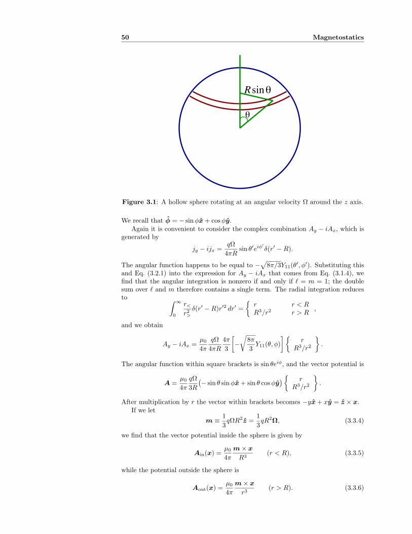
50 Magnetostatics
R sinθ
θ
Figure 3.1: A hollow sphere rotating at an angular velocity Ω around the z axis.
We recall that φ = − sin φx + cos φy.Again it is convenient to consider the complex combination Ay − iAx, which is
generated by
jy − ijx =qΩ
4πRsin θ′eiφ′
δ(r′ − R).
The angular function happens to be equal to −0
8π/3Y11(θ′,φ′). Substituting thisand Eq. (3.2.1) into the expression for Ay − iAx that comes from Eq. (3.1.4), wefind that the angular integration is nonzero if and only if ℓ = m = 1; the doublesum over ℓ and m therefore contains a single term. The radial integration reducesto
! ∞
0
r<
r2>
δ(r′ − R)r′2 dr′ =
8
r r < RR3/r2 r > R
,
and we obtain
Ay − iAx =µ0
4π
qΩ
4πR
4π
3
3
−5
8π
3Y11(θ,φ)
4 8
rR3/r2
9
.
The angular function within square brackets is sin θeiφ, and the vector potential is
A =µ0
4π
qΩ
3R
%
− sin θ sin φx + sin θ cos φy&
8
rR3/r2
9
.
After multiplication by r the vector within brackets becomes −yx + xy = z × x.If we let
m ≡1
3qΩR2z =
1
3qR2Ω, (3.3.4)
we find that the vector potential inside the sphere is given by
Ain(x) =µ0
4π
m × x
R3(r < R), (3.3.5)
while the potential outside the sphere is
Aout(x) =µ0
4π
m × x
r3(r > R). (3.3.6)
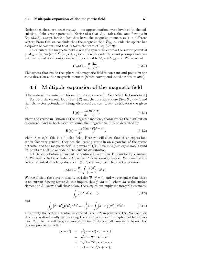
3.4 Multipole expansion of the magnetic field 51
Notice that these are exact results — no approximations were involved in the cal-culation of the vector potential. Notice also that Aout takes the same form as inEq. (3.2.8), except for the fact that here, the magnetic moment m is a differentvector. From this we conclude that the magnetic field Bout outside the sphere hasa dipolar behaviour, and that it takes the form of Eq. (3.2.9).
To calculate the magnetic field inside the sphere we express the vector potentialas Ain = (µ0/4π)(m/R3)(−yx + xy) and take its curl. Its x and y components areboth zero, and its z component is proportional to ∇xx + ∇yy = 2. We arrive at
Bin(x) =µ0
4π
2m
R3. (3.3.7)
This states that inside the sphere, the magnetic field is constant and points in thesame direction as the magnetic moment (which corresponds to the rotation axis).
3.4 Multipole expansion of the magnetic field
[The material presented in this section is also covered in Sec. 5.6 of Jackson’s text.]For both the current loop (Sec. 3.2) and the rotating sphere (Sec. 3.3) we found
that the vector potential at a large distance from the current distribution was givenby
A(x) =µ0
4π
m × x
r3, (3.4.1)
where the vector m, known as the magnetic moment, characterizes the distributionof current. And in both cases we found the magnetic field to be described by
B(x) =µ0
4π
3(m · r)r − m
r3, (3.4.2)
where r = x/r; this is a dipolar field. Here we will show that these expressionsare in fact very general: they are the leading terms in an expansion of the vectorpotential and the magnetic field in powers of 1/r. This multipole expansion is validfor points x that lie outside of the current distribution.
Let the distribution of current be confined to a volume V bounded by a surfaceS. We take x to be outside of V , while x′ is necessarily inside. We examine thevector potential at a large distance r ≫ r′, starting from the exact expression
A(x) =µ0
4π
!
j(x′)
|x − x′|d3x′.
We recall that the current density satisfies ∇ · j = 0, and we recognize that thereis no current flowing across S; this implies that j · da = 0, where da is the surfaceelement on S. As we shall show below, these equations imply the integral statements
!
Vj(x′) d3x′ = 0 (3.4.3)
and!
V
%
r · x′&
j(x′) d3x′ = −1
2r ×
!
V
'
x′ × j(x′)(
d3x′. (3.4.4)
To simplify the vector potential we expand 1/|x−x′| in powers of 1/r. We could dothis very systematically by involving the addition theorem for spherical harmonics(Sec. 2.6), but it will be good enough to keep only a small number of terms. Forthis we proceed directly:
|x − x′| =0
(x − x′) · (x − x′)
=0
r2 − 2x · x′ − r′2
= r0
1 − 2r · x′/r + · · ·= r
%
1 − r · x′/r + · · ·&
,
52 Magnetostatics
so that1
|x − x′|=
1
r
,
1 + r · x′/r + · · ·-
.
Substituting this into the exact expression for A(x) gives
A(x) =µ0
4π
3
1
r
!
Vj(x′) d3x′ +
1
r2
!
V
%
r · x′&
j(x′) d3x′ + · · ·4
.
The first term on the right-hand side vanishes by virtue of Eq. (3.4.3), and thesecond term is altered by Eq. (3.4.4). We have
A(x) =µ0
4π
1
r2
8
−1
2r ×
!
V
'
x′ × j(x′)(
d3x′ + · · ·9
,
and if we define the magnetic moment of the current distribution by
m =1
2
!
Vx′ × j(x′) d3x′, (3.4.5)
then we recover Eq. (3.4.1). We see that indeed,
A(x) =µ0
4π
m × r
r2+ O
"
1
r3
#
is a very general expression, and that the magnetic moment of an arbitrary distri-bution of current is given by Eq. (3.4.5). It is a straightforward exercise to showthat for the current loop of Sec. 3.2, Eq. (3.4.5) reproduces Eq. (3.2.7). Similarly,Eq. (3.4.5) reduces to Eq. (3.3.4) for the rotating sphere of Sec. 3.3.
We still have to establish the identities of Eqs. (3.4.3) and (3.4.4). We beginwith the z component of Eq. (3.4.3), in which we drop the primes on the integrationvariables. Consider
∇ · (zj) = z(∇ · j) + j · ∇z = jz,
which follows because ∇ ·j = 0 and ∇z = z. Integrating this equation over V gives
!
Vjz d3x =
!
V∇ · (zj) d3x =
)
Szj · da,
where we have invoked Gauss’ theorem. But the right-hand side is zero because nocurrent crosses the surface S, and we have
*
V jz d3x = 0. Proceeding similarly withthe x and y components, we arrive at Eq. (3.4.3).
To establish Eq. (3.4.4) requires a bit more work, but the idea is the same. Weconsider the z component of this equation, in which we drop the primes on theintegration variables. (At the same time we replace the vector r, which is constantwith respect to the primed variables, by an arbitrary constant vector e.) We have
!
V
%
e · x&
jz d3x = ex
!
Vxjz d3x + ey
!
Vyjz d3x + ez
!
Vzjz d3x
for the left-hand side of the identity. Consider now
∇ · (xzj) = xz(∇ · j) + j · ∇(xz) = xjz + zjx,
which integrates to
!
V(xjz + zjx) d3x =
)
Sxzj · da = 0,
3.5 Problems 53
giving rise to the integral identity!
Vxjz d3x = −
!
Vzjx d3x.
Similarly,!
Vyjz d3x = −
!
Vzjy d3x.
On the other hand,
∇ · (z2j) = z2(∇ · j) + j · ∇z2 = 2zjz,
and this yields!
Vzjz d3x = 0.
Using these results, we go back to the left-hand side of Eq. (3.4.4) and write
!
V
%
e · x&
jz d3x =1
2ex
"!
Vxjz d3x −
!
Vzjx d3x
#
+1
2ey
"!
Vyjz d3x −
!
Vzjy d3x
#
= −1
2ex
!
V(zjx − xjz) d3x +
1
2ey
!
V(yjz − zjy) d3x.
Inside the first integral we recognize the y component of the vector x× j, while thesecond integral contains its x component. So
!
V
%
e · x&
jz d3x = −1
2
"
ex
!
V(x × j)y d3x − ey
!
V(x × j)x d3x
#
= −1
2
"
e ×!
V(x × j) d3x
#
z
,
and we have arrived at the right-hand side of Eq. (3.4.4).
3.5 Problems
1. Show that for the current loop of Sec. 3.2, Eq. (3.4.5) reproduces Eq. (3.2.7).And show that Eq. (3.4.5) reduces to Eq. (3.3.4) for the rotating sphere ofSec. 3.3.
2. A uniformly charged sphere of radius R is rotating around the z axis withan angular velocity Ω. Take the density of charge inside the sphere to be3q/(4πR3) (for r < R), where q is the sphere’s total charge. Calculate m, thesphere’s magnetic moment vector.
3. Calculate the vector potential A(x) inside the spinning sphere of the precedingproblem. Express it in terms of the sphere’s magnetic moment vector m.
4. Prove that for a current loop of arbitrary shape that lies in a plane, Eq. (3.4.5)gives
|m| = (current)(area enclosed by loop),
and that the direction of m is normal to the plane.

54 Magnetostatics
Chapter 4
Electromagnetic waves in
matter
4.1 Macroscopic form of Maxwell’s equations
[The material presented in this section is also covered in Sec. 6.6 of Jackson’s text.]Our goal in this chapter is to describe how electromagnetic waves propagate in
dielectric materials. Our first task will be to reformulate Maxwell’s equations in away that conveniently incorporates the electromagnetic response of the medium.
4.1.1 Microscopic and macroscopic quantities
Maxwell’s equations, as they were written down in Chapter 1, are the fundamentalequations of classical electrodynamics; in principle they require no modificationeven in the presence of a nontrivial medium. But it is convenient to write themin a different form, in which the charges that are free to move within the mediumare distinguished from the charges that are tied to the medium’s molecules, and inwhich the microscopic fluctuations of all the variables involved have been smoothedout. The resulting form of Maxwell’s equations involves only macroscopic densitiesof free charges and currents, and macroscopic electromagnetic fields.
To distinguish them from macroscopic quantities, the fundamental, microscopicvariables will be assigned different symbols in this chapter. The microscopic densityof charge (including both free and bound charges) is denoted η, while the micro-scopic density of current (including both free and bound currents) is denoted J .The microscopic electric field is denoted e, and the microscopic magnetic field isdenoted b. These quantities are related by the microscopic Maxwell equations,
∇ · e =1
ϵ0η, (4.1.1)
∇ · b = 0, (4.1.2)
∇ × e +∂b
∂t= 0, (4.1.3)
∇ × b − ϵ0µ0∂e
∂t= µ0J , (4.1.4)
which are the same as in Chapter 1. The macroscopic density of free charge will bedenoted ρ, while the macroscopic density of free current will be denoted j. Theseare obtained from the microscopic quantities by removing the contribution fromthe bound charges (those that are tied to the molecules and become part of themedium’s electromagnetic response) and by macroscopic smoothing; the preciserelationships will be given below. The macroscopic fields will be denoted E, D,
55
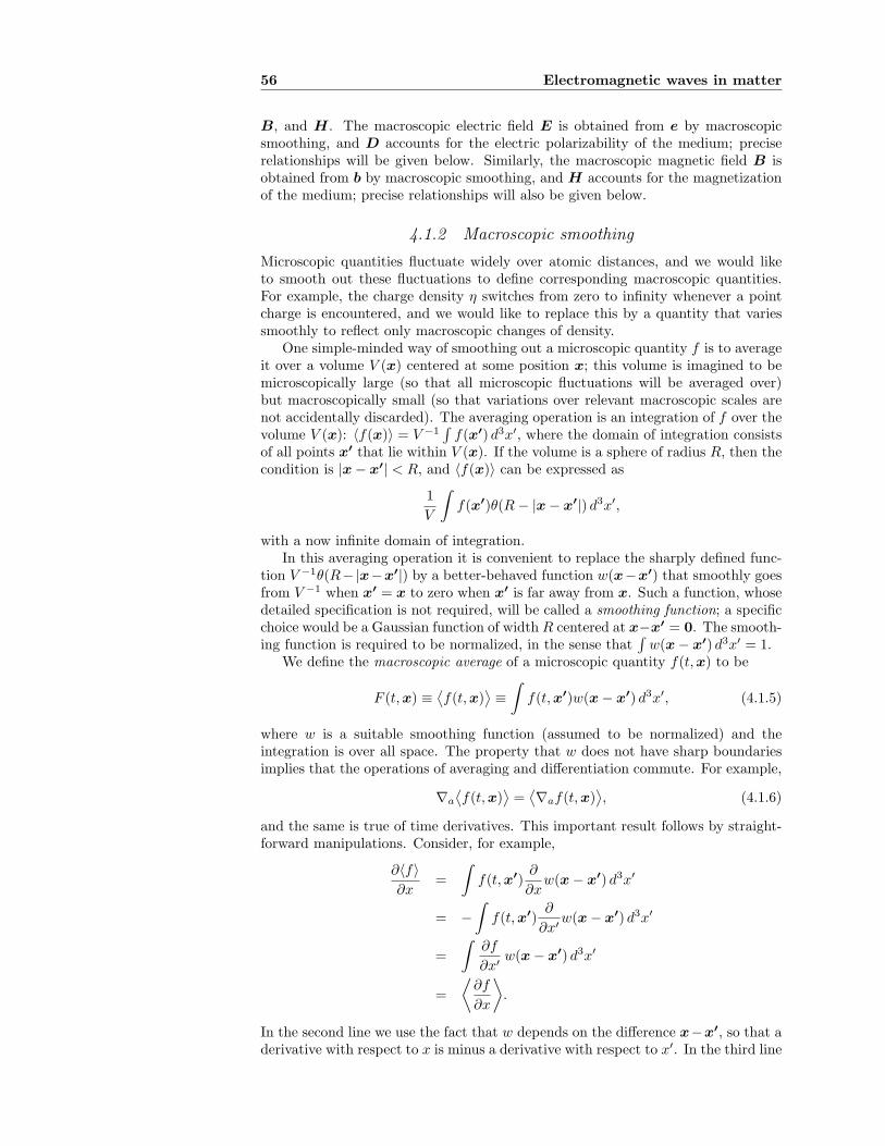
56 Electromagnetic waves in matter
B, and H. The macroscopic electric field E is obtained from e by macroscopicsmoothing, and D accounts for the electric polarizability of the medium; preciserelationships will be given below. Similarly, the macroscopic magnetic field B isobtained from b by macroscopic smoothing, and H accounts for the magnetizationof the medium; precise relationships will also be given below.
4.1.2 Macroscopic smoothing
Microscopic quantities fluctuate widely over atomic distances, and we would liketo smooth out these fluctuations to define corresponding macroscopic quantities.For example, the charge density η switches from zero to infinity whenever a pointcharge is encountered, and we would like to replace this by a quantity that variessmoothly to reflect only macroscopic changes of density.
One simple-minded way of smoothing out a microscopic quantity f is to averageit over a volume V (x) centered at some position x; this volume is imagined to bemicroscopically large (so that all microscopic fluctuations will be averaged over)but macroscopically small (so that variations over relevant macroscopic scales arenot accidentally discarded). The averaging operation is an integration of f over thevolume V (x): ⟨f(x)⟩ = V −1
*
f(x′) d3x′, where the domain of integration consistsof all points x′ that lie within V (x). If the volume is a sphere of radius R, then thecondition is |x − x′| < R, and ⟨f(x)⟩ can be expressed as
1
V
!
f(x′)θ(R − |x − x′|) d3x′,
with a now infinite domain of integration.In this averaging operation it is convenient to replace the sharply defined func-
tion V −1θ(R− |x−x′|) by a better-behaved function w(x−x′) that smoothly goesfrom V −1 when x′ = x to zero when x′ is far away from x. Such a function, whosedetailed specification is not required, will be called a smoothing function; a specificchoice would be a Gaussian function of width R centered at x−x′ = 0. The smooth-ing function is required to be normalized, in the sense that
*
w(x − x′) d3x′ = 1.We define the macroscopic average of a microscopic quantity f(t,x) to be
F (t,x) ≡:
f(t,x);
≡!
f(t,x′)w(x − x′) d3x′, (4.1.5)
where w is a suitable smoothing function (assumed to be normalized) and theintegration is over all space. The property that w does not have sharp boundariesimplies that the operations of averaging and differentiation commute. For example,
∇a
:
f(t,x);
=:
∇af(t,x);
, (4.1.6)
and the same is true of time derivatives. This important result follows by straight-forward manipulations. Consider, for example,
∂⟨f⟩∂x
=
!
f(t,x′)∂
∂xw(x − x′) d3x′
= −!
f(t,x′)∂
∂x′w(x − x′) d3x′
=
!
∂f
∂x′w(x − x′) d3x′
=
<
∂f
∂x
=
.
In the second line we use the fact that w depends on the difference x−x′, so that aderivative with respect to x is minus a derivative with respect to x′. In the third line
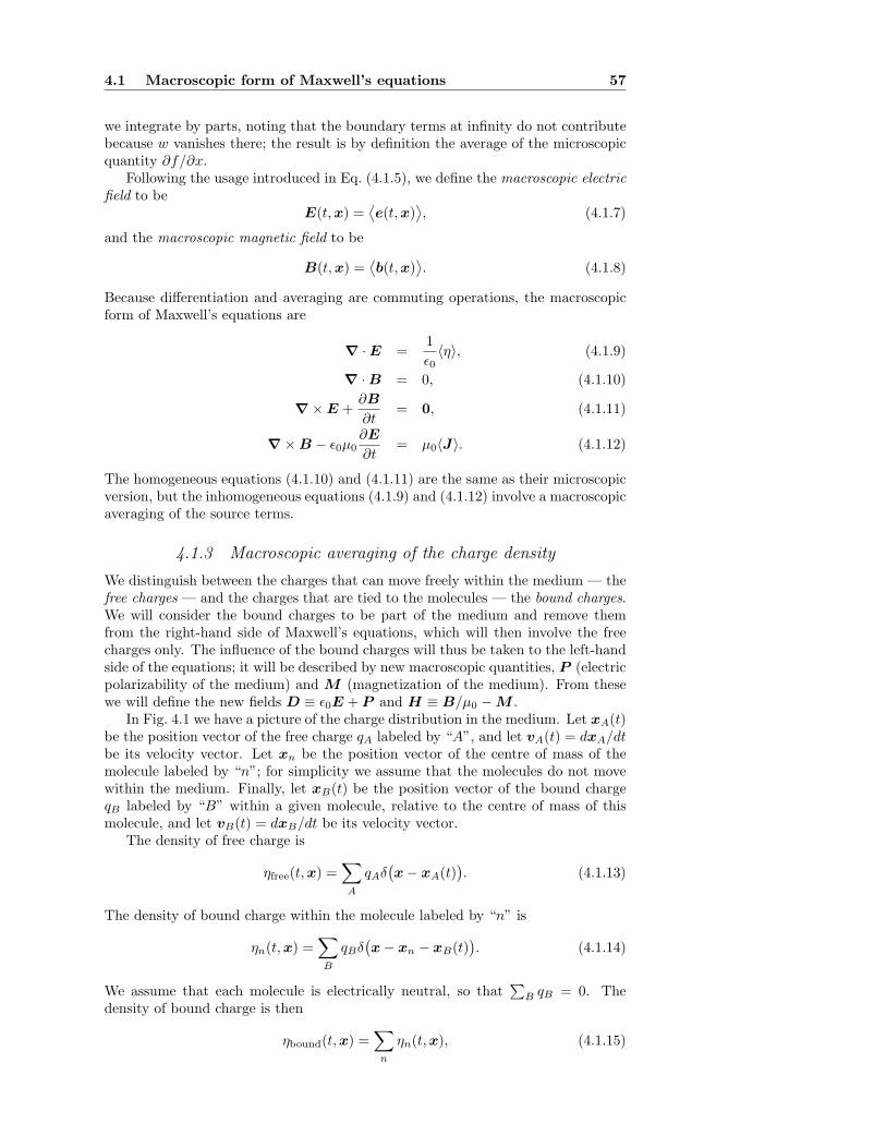
4.1 Macroscopic form of Maxwell’s equations 57
we integrate by parts, noting that the boundary terms at infinity do not contributebecause w vanishes there; the result is by definition the average of the microscopicquantity ∂f/∂x.
Following the usage introduced in Eq. (4.1.5), we define the macroscopic electricfield to be
E(t,x) =:
e(t,x);
, (4.1.7)
and the macroscopic magnetic field to be
B(t,x) =:
b(t,x);
. (4.1.8)
Because differentiation and averaging are commuting operations, the macroscopicform of Maxwell’s equations are
∇ · E =1
ϵ0⟨η⟩, (4.1.9)
∇ · B = 0, (4.1.10)
∇ × E +∂B
∂t= 0, (4.1.11)
∇ × B − ϵ0µ0∂E
∂t= µ0⟨J⟩. (4.1.12)
The homogeneous equations (4.1.10) and (4.1.11) are the same as their microscopicversion, but the inhomogeneous equations (4.1.9) and (4.1.12) involve a macroscopicaveraging of the source terms.
4.1.3 Macroscopic averaging of the charge density
We distinguish between the charges that can move freely within the medium — thefree charges — and the charges that are tied to the molecules — the bound charges.We will consider the bound charges to be part of the medium and remove themfrom the right-hand side of Maxwell’s equations, which will then involve the freecharges only. The influence of the bound charges will thus be taken to the left-handside of the equations; it will be described by new macroscopic quantities, P (electricpolarizability of the medium) and M (magnetization of the medium). From thesewe will define the new fields D ≡ ϵ0E + P and H ≡ B/µ0 − M .
In Fig. 4.1 we have a picture of the charge distribution in the medium. Let xA(t)be the position vector of the free charge qA labeled by “A”, and let vA(t) = dxA/dtbe its velocity vector. Let xn be the position vector of the centre of mass of themolecule labeled by “n”; for simplicity we assume that the molecules do not movewithin the medium. Finally, let xB(t) be the position vector of the bound chargeqB labeled by “B” within a given molecule, relative to the centre of mass of thismolecule, and let vB(t) = dxB/dt be its velocity vector.
The density of free charge is
ηfree(t,x) =$
A
qAδ%
x − xA(t)&
. (4.1.13)
The density of bound charge within the molecule labeled by “n” is
ηn(t,x) =$
B
qBδ%
x − xn − xB(t)&
. (4.1.14)
We assume that each molecule is electrically neutral, so that>
B qB = 0. Thedensity of bound charge is then
ηbound(t,x) =$
n
ηn(t,x), (4.1.15)
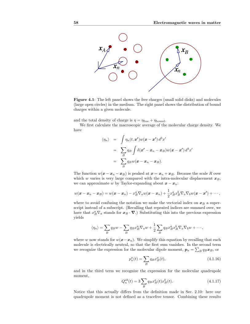
58 Electromagnetic waves in matter
x
x x
x
n
A B
n
Figure 4.1: The left panel shows the free charges (small solid disks) and molecules(large open circles) in the medium. The right panel shows the distribution of boundcharges within a given molecule.
and the total density of charge is η = ηfree + ηbound.We first calculate the macroscopic average of the molecular charge density. We
have
⟨ηn⟩ =
!
ηn(t,x′)w(x − x′) d3x′
=$
B
qB
!
δ(x′ − xn − xB)w(x − x′) d3x′
=$
B
qBw(x − xn − xB).
The function w(x−xn −xB) is peaked at x = xn + xB. Because the scale R overwhich w varies is very large compared with the intra-molecular displacement xB ,we can approximate w by Taylor-expanding about x − xn:
w(x − xn − xB) = w(x − xn) − xaB∇aw(x − xn) +
1
2xa
BxbB∇a∇bw(x − x′) + · · · ,
where to avoid confusing the notation we make the vectorial index on xB a super-script instead of a subscript. (Recalling that repeated indices are summed over, wehave that xa
B∇a stands for xB · ∇.) Substituting this into the previous expressionyields
⟨ηn⟩ =$
B
qBw −$
B
qBxaB∇aw +
1
2
$
B
qBxaBxb
B∇a∇bw + · · · ,
where w now stands for w(x−xn). We simplify this equation by recalling that eachmolecule is electrically neutral, so that the first sum vanishes. In the second termwe recognize the expression for the molecular dipole moment, pn =
>
B qBxB, or
pan(t) =
$
B
qBxaB(t), (4.1.16)
and in the third term we recognize the expression for the molecular quadrupolemoment,
Qabn (t) = 3
$
B
qBxaB(t)xb
B(t). (4.1.17)
Notice that this actually differs from the definition made in Sec. 2.10: here ourquadrupole moment is not defined as a tracefree tensor. Combining these results
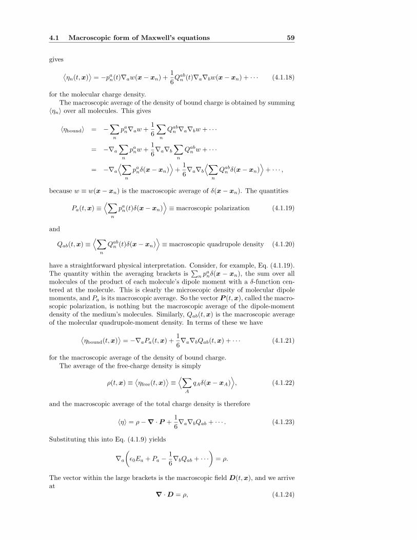
4.1 Macroscopic form of Maxwell’s equations 59
gives
:
ηn(t,x);
= −pan(t)∇aw(x − xn) +
1
6Qab
n (t)∇a∇bw(x − xn) + · · · (4.1.18)
for the molecular charge density.The macroscopic average of the density of bound charge is obtained by summing
⟨ηn⟩ over all molecules. This gives
⟨ηbound⟩ = −$
n
pan∇aw +
1
6
$
n
Qabn ∇a∇bw + · · ·
= −∇a
$
n
panw +
1
6∇a∇b
$
n
Qabn w + · · ·
= −∇a
?
$
n
panδ(x − xn)
@
+1
6∇a∇b
?
$
n
Qabn δ(x − xn)
@
+ · · · ,
because w ≡ w(x − xn) is the macroscopic average of δ(x − xn). The quantities
Pa(t,x) ≡?
$
n
pan(t)δ(x − xn)
@
≡ macroscopic polarization (4.1.19)
and
Qab(t,x) ≡?
$
n
Qabn (t)δ(x − xn)
@
≡ macroscopic quadrupole density (4.1.20)
have a straightforward physical interpretation. Consider, for example, Eq. (4.1.19).The quantity within the averaging brackets is
>
n panδ(x − xn), the sum over all
molecules of the product of each molecule’s dipole moment with a δ-function cen-tered at the molecule. This is clearly the microscopic density of molecular dipolemoments, and Pa is its macroscopic average. So the vector P (t,x), called the macro-scopic polarization, is nothing but the macroscopic average of the dipole-momentdensity of the medium’s molecules. Similarly, Qab(t,x) is the macroscopic averageof the molecular quadrupole-moment density. In terms of these we have
:
ηbound(t,x);
= −∇aPa(t,x) +1
6∇a∇bQab(t,x) + · · · (4.1.21)
for the macroscopic average of the density of bound charge.The average of the free-charge density is simply
ρ(t,x) ≡:
ηfree(t,x);
≡?
$
A
qAδ(x − xA)@
, (4.1.22)
and the macroscopic average of the total charge density is therefore
⟨η⟩ = ρ − ∇ · P +1
6∇a∇bQab + · · · . (4.1.23)
Substituting this into Eq. (4.1.9) yields
∇a
"
ϵ0Ea + Pa −1
6∇bQab + · · ·
#
= ρ.
The vector within the large brackets is the macroscopic field D(t,x), and we arriveat
∇ · D = ρ, (4.1.24)
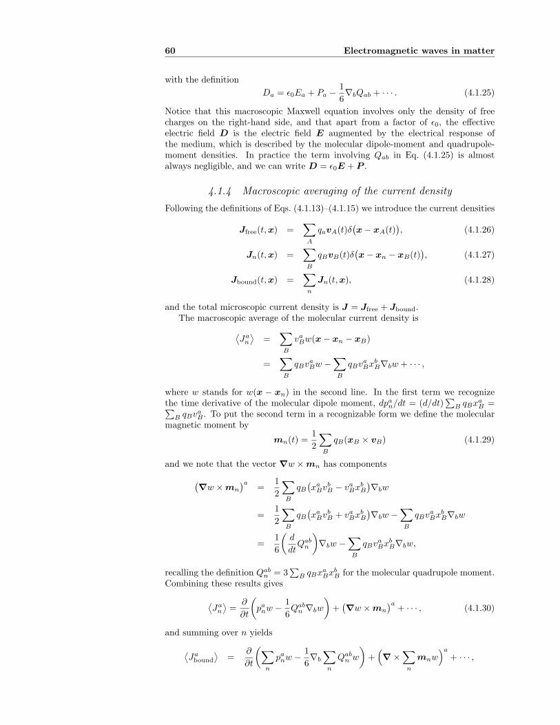
60 Electromagnetic waves in matter
with the definition
Da = ϵ0Ea + Pa −1
6∇bQab + · · · . (4.1.25)
Notice that this macroscopic Maxwell equation involves only the density of freecharges on the right-hand side, and that apart from a factor of ϵ0, the effectiveelectric field D is the electric field E augmented by the electrical response ofthe medium, which is described by the molecular dipole-moment and quadrupole-moment densities. In practice the term involving Qab in Eq. (4.1.25) is almostalways negligible, and we can write D = ϵ0E + P .
4.1.4 Macroscopic averaging of the current density
Following the definitions of Eqs. (4.1.13)–(4.1.15) we introduce the current densities
Jfree(t,x) =$
A
qavA(t)δ%
x − xA(t)&
, (4.1.26)
Jn(t,x) =$
B
qBvB(t)δ%
x − xn − xB(t)&
, (4.1.27)
Jbound(t,x) =$
n
Jn(t,x), (4.1.28)
and the total microscopic current density is J = Jfree + Jbound.The macroscopic average of the molecular current density is
:
Jan
;
=$
B
vaBw(x − xn − xB)
=$
B
qBvaBw −
$
B
qBvaBxb
B∇bw + · · · ,
where w stands for w(x − xn) in the second line. In the first term we recognizethe time derivative of the molecular dipole moment, dpa
n/dt = (d/dt)>
B qBxaB =
>
B qBvaB. To put the second term in a recognizable form we define the molecular
magnetic moment by
mn(t) =1
2
$
B
qB(xB × vB) (4.1.29)
and we note that the vector ∇w × mn has components
%
∇w × mn
&a=
1
2
$
B
qB
%
xaBvb
B − vaBxb
B
&
∇bw
=1
2
$
B
qB
%
xaBvb
B + vaBxb
B
&
∇bw −$
B
qBvaBxb
B∇bw
=1
6
"
d
dtQab
n
#
∇bw −$
B
qBvaBxb
B∇bw,
recalling the definition Qabn = 3
>
B qBxaBxb
B for the molecular quadrupole moment.Combining these results gives
:
Jan
;
=∂
∂t
"
panw −
1
6Qab
n ∇bw
#
+%
∇w × mn
&a+ · · · , (4.1.30)
and summing over n yields
:
Jabound
;
=∂
∂t
"
$
n
panw −
1
6∇b
$
n
Qabn w
#
+,
∇ ×$
n
mnw-a
+ · · · ,
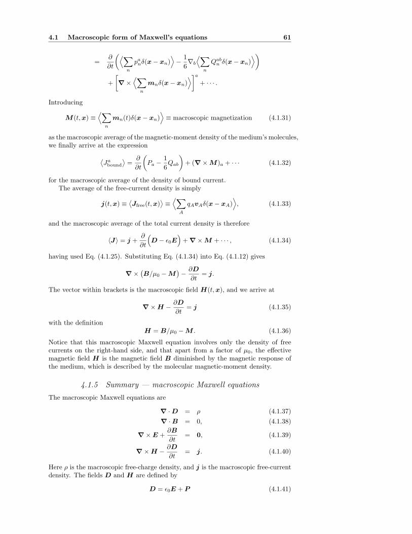
4.1 Macroscopic form of Maxwell’s equations 61
=∂
∂t
"
?
$
n
panδ(x − xn)
@
−1
6∇b
?
$
n
Qabn δ(x − xn)
@
#
+
3
∇ ×?
$
n
mnδ(x − xn)@
4a
+ · · · .
Introducing
M(t,x) ≡?
$
n
mn(t)δ(x − xn)@
≡ macroscopic magnetization (4.1.31)
as the macroscopic average of the magnetic-moment density of the medium’s molecules,we finally arrive at the expression
:
Jabound
;
=∂
∂t
"
Pa −1
6Qab
#
+ (∇ × M)a + · · · (4.1.32)
for the macroscopic average of the density of bound current.The average of the free-current density is simply
j(t,x) ≡:
Jfree(t,x);
≡?
$
A
qAvAδ(x − xA)@
, (4.1.33)
and the macroscopic average of the total current density is therefore
⟨J⟩ = j +∂
∂t
,
D − ϵ0E-
+ ∇ × M + · · · , (4.1.34)
having used Eq. (4.1.25). Substituting Eq. (4.1.34) into Eq. (4.1.12) gives
∇ ×%
B/µ0 − M&
−∂D
∂t= j.
The vector within brackets is the macroscopic field H(t,x), and we arrive at
∇ × H −∂D
∂t= j (4.1.35)
with the definitionH = B/µ0 − M . (4.1.36)
Notice that this macroscopic Maxwell equation involves only the density of freecurrents on the right-hand side, and that apart from a factor of µ0, the effectivemagnetic field H is the magnetic field B diminished by the magnetic response ofthe medium, which is described by the molecular magnetic-moment density.
4.1.5 Summary — macroscopic Maxwell equations
The macroscopic Maxwell equations are
∇ · D = ρ (4.1.37)
∇ · B = 0, (4.1.38)
∇ × E +∂B
∂t= 0, (4.1.39)
∇ × H −∂D
∂t= j. (4.1.40)
Here ρ is the macroscopic free-charge density, and j is the macroscopic free-currentdensity. The fields D and H are defined by
D = ϵ0E + P (4.1.41)
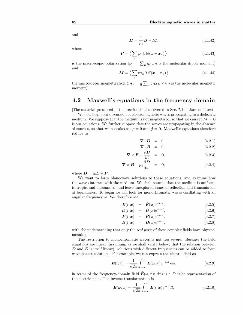
62 Electromagnetic waves in matter
and
H =1
µ0B − M , (4.1.42)
whereP =
?
$
n
pn(t)δ(x − xn)@
(4.1.43)
is the macroscopic polarization (pn =>
B qBxB is the molecular dipole moment)and
M =?
$
n
mn(t)δ(x − xn)@
(4.1.44)
the macroscopic magnetization (mn = 12
>
B qBxB × vB is the molecular magneticmoment).
4.2 Maxwell’s equations in the frequency domain
[The material presented in this section is also covered in Sec. 7.1 of Jackson’s text.]We now begin our discussion of electromagnetic waves propagating in a dielectric
medium. We suppose that the medium is not magnetized, so that we can set M = 0is our equations. We further suppose that the waves are propagating in the absenceof sources, so that we can also set ρ = 0 and j = 0. Maxwell’s equations thereforereduce to
∇ · D = 0 (4.2.1)
∇ · B = 0, (4.2.2)
∇ × E +∂B
∂t= 0, (4.2.3)
∇ × B − µ0∂D
∂t= 0, (4.2.4)
where D = ϵ0E + P .We want to form plane-wave solutions to these equations, and examine how
the waves interact with the medium. We shall assume that the medium is uniform,isotropic, and unbounded, and leave unexplored issues of reflection and transmissionat boundaries. To begin we will look for monochromatic waves oscillating with anangular frequency ω. We therefore set
E(t,x) = E(x)e−iωt, (4.2.5)
D(t,x) = D(x)e−iωt, (4.2.6)
P (t,x) = P (x)e−iωt, (4.2.7)
B(t,x) = B(x)e−iωt, (4.2.8)
with the understanding that only the real parts of these complex fields have physicalmeaning.
The restriction to monochromatic waves is not too severe. Because the fieldequations are linear (assuming, as we shall verify below, that the relation betweenD and E is itself linear), solutions with different frequencies can be added to formwave-packet solutions. For example, we can express the electric field as
E(t,x) =1√2π
! ∞
−∞E(ω,x)e−iωt dω, (4.2.9)
in terms of the frequency-domain field E(ω,x); this is a Fourier representation ofthe electric field. The inverse transformation is
E(ω,x) =1√2π
! ∞
−∞E(t,x)eiωt dt, (4.2.10)
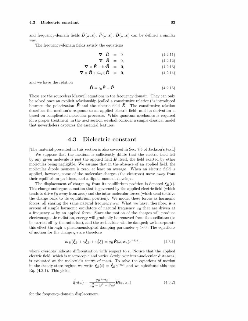
4.3 Dielectric constant 63
and frequency-domain fields D(ω,x), P (ω,x), B(ω,x) can be defined a similarway.
The frequency-domain fields satisfy the equations
∇ · D = 0 (4.2.11)
∇ · B = 0, (4.2.12)
∇ × E − iωB = 0, (4.2.13)
∇ × B + iωµ0D = 0, (4.2.14)
and we have the relation
D = ϵ0E + P . (4.2.15)
These are the sourceless Maxwell equations in the frequency domain. They can onlybe solved once an explicit relationship (called a constitutive relation) is introducedbetween the polarization P and the electric field E. The constitutive relationdescribes the medium’s response to an applied electric field, and its derivation isbased on complicated molecular processes. While quantum mechanics is requiredfor a proper treatment, in the next section we shall consider a simple classical modelthat nevertheless captures the essential features.
4.3 Dielectric constant
[The material presented in this section is also covered in Sec. 7.5 of Jackson’s text.]We suppose that the medium is sufficiently dilute that the electric field felt
by any given molecule is just the applied field E itself, the field exerted by othermolecules being negligible. We assume that in the absence of an applied field, themolecular dipole moment is zero, at least on average. When an electric field isapplied, however, some of the molecular charges (the electrons) move away fromtheir equilibrium positions, and a dipole moment develops.
The displacement of charge qB from its equilibrium position is denoted ξB(t).This charge undergoes a motion that is governed by the applied electric field (whichtends to drive ξB away from zero) and the intra-molecular forces (which tend to drivethe charge back to its equilibrium position). We model these forces as harmonicforces, all sharing the same natural frequency ω0. What we have, therefore, is asystem of simple harmonic oscillators of natural frequency ω0 that are driven ata frequency ω by an applied force. Since the motion of the charges will produceelectromagnetic radiation, energy will gradually be removed from the oscillators (tobe carried off by the radiation), and the oscillations will be damped; we incorporatethis effect through a phenomenological damping parameter γ > 0. The equationsof motion for the charge qB are therefore
mB
%
ξB + γξB + ω20ξ
&
= qBE(ω,xn)e−iωt, (4.3.1)
where overdots indicate differentiation with respect to t. Notice that the appliedelectric field, which is macroscopic and varies slowly over intra-molecular distances,is evaluated at the molecule’s centre of mass. To solve the equations of motionin the steady-state regime we write ξB(t) = ξBe−iωt and we substitute this intoEq. (4.3.1). This yields
ξB(ω) =qB/mB
ω20 − ω2 − iγω
E(ω,xn) (4.3.2)
for the frequency-domain displacement.
64 Electromagnetic waves in matter
The molecule’s dipole moment is pn =>
B qB(xB + ξB), where xB is the equi-librium position of charge qB . Because the dipole moment vanishes at equilibrium,this reduces to pn =
>
B qBξB . Substituting Eq. (4.3.2) then gives
pn =$
B
q2B/mB
ω20 − ω2 − iγω
E(ω,xn).
Since all the contributing charges qB are electrons, we can write>
B q2B/mB =
Ze2/m, where Z is the number of electrons per molecule, e the electronic charge,and m the electron’s mass. We therefore arrive at
pn(ω) =Ze2
m
1
ω20 − ω2 − iγω
E(ω,xn) (4.3.3)
for the molecular dipole moment in the frequency domain.The polarization vector is then
P =?
$
n
pnδ(x − xn)@
=Ze2
m
1
ω20 − ω2 − iγω
?
$
n
E(ω,xn)δ(x − xn)@
=Ze2
m
1
ω20 − ω2 − iγω
E(ω,x)?
$
n
δ(x − xn)@
.
The quantity within the averaging brackets is the microscopic molecular density. Itsmacroscopic average is therefore the medium’s density N (the number of moleculesper macroscopic unit volume), which we take to be uniform. We have arrived at
P (ω,x) =Ze2N
m
1
ω20 − ω2 − iγω
E(ω,x) (4.3.4)
for the frequency-domain polarization. We recall that Z is the number of electronsper molecule, that N is the molecular number density, and that e and m are theelectron’s charge and mass, respectively. We notice that the relationship betweenP and E is linear, as was anticipated in Sec. 4.2.
The relationship between D ≡ ϵ0E + P and E also is linear. We express it as
D = ϵ0
"
1 +Ze2N
ϵ0m
1
ω20 − ω2 − iγω
#
E,
or asD(ω,x) = ϵ(ω)E(ω,x), (4.3.5)
having introduced the (complex, and frequency-dependent) dielectric constant
ϵ(ω)
ϵ0= 1 +
ω2p
ω20 − ω2 − iγω
(4.3.6)
and the medium’s plasma frequency
ωp =
"
Ze2N
ϵ0m
#1/2
. (4.3.7)
Equation (4.3.6) is the product of a simplistic classical model. But a properquantum-mechanical treatment would produce a similar result, except for the fact
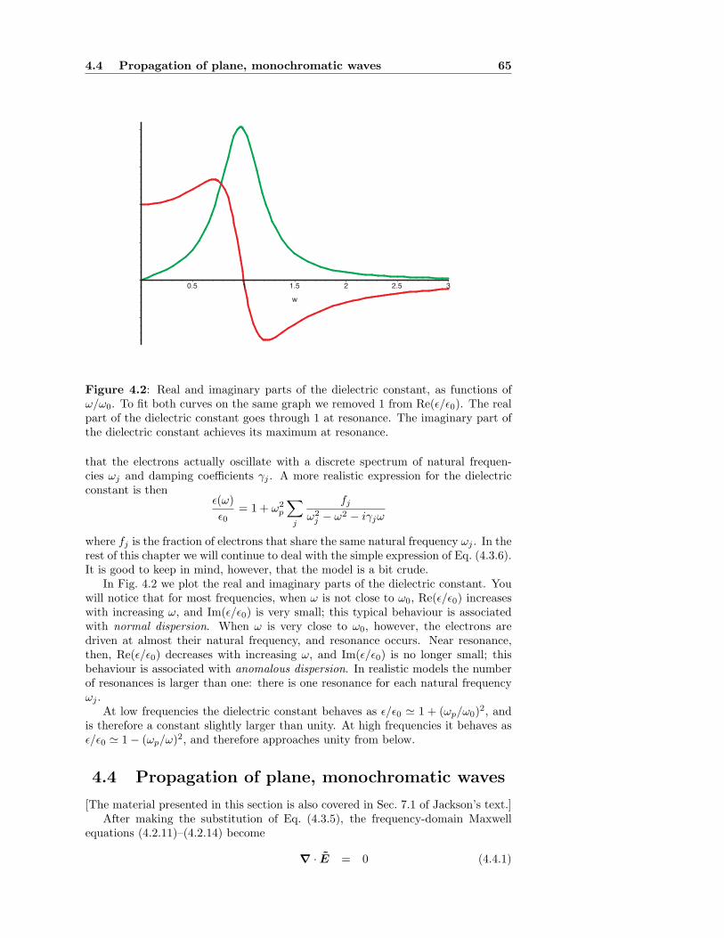
4.4 Propagation of plane, monochromatic waves 65
0.5 1 1.5 2 2.5 3
w
Figure 4.2: Real and imaginary parts of the dielectric constant, as functions ofω/ω0. To fit both curves on the same graph we removed 1 from Re(ϵ/ϵ0). The realpart of the dielectric constant goes through 1 at resonance. The imaginary part ofthe dielectric constant achieves its maximum at resonance.
that the electrons actually oscillate with a discrete spectrum of natural frequen-cies ωj and damping coefficients γj . A more realistic expression for the dielectricconstant is then
ϵ(ω)
ϵ0= 1 + ω2
p
$
j
fj
ω2j − ω2 − iγjω
where fj is the fraction of electrons that share the same natural frequency ωj . In therest of this chapter we will continue to deal with the simple expression of Eq. (4.3.6).It is good to keep in mind, however, that the model is a bit crude.
In Fig. 4.2 we plot the real and imaginary parts of the dielectric constant. Youwill notice that for most frequencies, when ω is not close to ω0, Re(ϵ/ϵ0) increaseswith increasing ω, and Im(ϵ/ϵ0) is very small; this typical behaviour is associatedwith normal dispersion. When ω is very close to ω0, however, the electrons aredriven at almost their natural frequency, and resonance occurs. Near resonance,then, Re(ϵ/ϵ0) decreases with increasing ω, and Im(ϵ/ϵ0) is no longer small; thisbehaviour is associated with anomalous dispersion. In realistic models the numberof resonances is larger than one: there is one resonance for each natural frequencyωj .
At low frequencies the dielectric constant behaves as ϵ/ϵ0 ≃ 1 + (ωp/ω0)2, andis therefore a constant slightly larger than unity. At high frequencies it behaves asϵ/ϵ0 ≃ 1 − (ωp/ω)2, and therefore approaches unity from below.
4.4 Propagation of plane, monochromatic waves
[The material presented in this section is also covered in Sec. 7.1 of Jackson’s text.]After making the substitution of Eq. (4.3.5), the frequency-domain Maxwell
equations (4.2.11)–(4.2.14) become
∇ · E = 0 (4.4.1)
66 Electromagnetic waves in matter
∇ · B = 0, (4.4.2)
∇ × E − iωB = 0, (4.4.3)
∇ × B + iωϵ(ω)µ0E = 0. (4.4.4)
We recall that the time-domain fields are reconstructed, for example, as E = Ee−iωt
if the wave is monochromatic, or as in Eq. (4.2.9) if the wave possesses a spectrumof frequencies.
It is easy to show that as a consequence of Eqs. (4.4.1)–(4.4.4), both E and B sat-isfy a frequency-domain wave equation. For example, taking the curl of Eq. (4.4.3)gives
∇ × (∇ × E) − iω∇ × B = 0;
substituting Eq. (4.4.4) and making use of the vectorial identity ∇ × (∇ × E) =∇(∇ · E) −∇2E puts this in the form
%
∇2 + k2&
E(ω,x) = 0, (4.4.5)
where
k2 ≡ω2
c2
ϵ(ω)
ϵ0. (4.4.6)
We have introduced a complex wave number k(ω), and we recall that c ≡ (ϵ0µ0)−1/2
is the speed of light in vacuum. Similar manipulations return
%
∇2 + k2&
B(ω,x) = 0, (4.4.7)
the statement that the magnetic field also satisfies a wave equation.To see how monochromatic electromagnetic waves propagate in a dielectric
medium, consider any component of E or B, and call it ψ. Then suppose thatthe wave is a plane wave that propagates in the z direction, so that ψ = ψ(z). Thewave equation simplifies to
"
d2
dz2+ k2
#
ψ(ω, z) = 0. (4.4.8)
A right-moving wave is described by the particular solution ψ = eikz. To helpidentify the physical properties of this wave we substitute Eq. (4.3.6) into Eq. (4.4.6)and get
k2 =ω2
c2
"
1 +ω2
p
ω20 − ω2 − iγω
#
. (4.4.9)
To be concrete we suppose that the second term within the large brackets is small.Taking the square root gives
k =ω
c
3
1 +ω2
p
2%
ω20 − ω2 − iγω
&
4
,
ork = kR + ikI , (4.4.10)
where
kR =ω
c
8
1 +ω2
p(ω20 − ω2)
2'
(ω20 − ω2)2 + γ2ω2
(
9
is the real part of the complex wave number, while
kI =ω
c
ω2cγω
2'
(ω20 − ω2)2 + γ2ω2
(
4.4 Propagation of plane, monochromatic waves 67
is its imaginary part.The right-moving wave is therefore described by
ψ(t, z) ≡ ψ(ω, z)e−iωt = e−kIze−i(ωt−kRz). (4.4.11)
From this expression we recognize that the wave is indeed traveling in the positivez direction, with a speed
vp =ω
kR(ω)≡
c
n(ω)(4.4.12)
known as the phase velocity; n ≡ ckR/ω is the medium’s index of refraction. Fromour previous expression for kR we obtain
n = 1 +ω2
p(ω20 − ω2)
2'
(ω20 − ω2)2 + γ2ω2
( ,
and we see that n ≃ 1 + 12 (ωp/ω0)2 > 1 for low frequencies, so that vp < c. On the
other hand, n ≃ 1 − 12 (ωp/ω)2 < 1 for high frequencies, so that vp > c. The phase
velocity of the wave can therefore exceed the speed of light in vacuum! This strangefact does not violate any cherished relativistic notion, because a monochromaticwave does not carry information. To form a signal one must modulate the waveand superpose solutions with different frequencies. As we shall see, in such situationsthe wave always travels with a speed that does not exceed c.
Another feature of Eq. (4.4.10) is that the wave is an exponentially decreasingfunction of z provided that kI is positive, which is guaranteed to be true if γ > 0.A positive damping constant means that some of the wave’s energy is dissipated bythe oscillating electrons (which emit their own electromagnetic radiation), and thewave must therefore decrease in amplitude as it travels through the medium. It isinteresting to note that in the case of lasers and masers, the electronic oscillationsactually reinforce the wave and lead to an exponential amplification instead of anattenuation; in such media the damping constant is negative.
Having constructed solutions to Eqs. (4.4.5) and (4.4.7), we should examinewhat constraints the full set of equations (4.4.1)–(4.4.4) place on these solutions.We write
E(ω, z) = eE0(ω)eik(ω)z (4.4.13)
andB(ω, z) = bB0(ω)eik(ω)z, (4.4.14)
where e and b are real unit vectors, and where E0 and B0 are complex amplitudes.Substituting these expressions into Eqs. (4.4.1) and (4.4.2) informs us that the unitvectors are both orthogonal to z,
e · z = b · z = 0; (4.4.15)
the fields are therefore transverse to the direction in which the wave propagates.Equation (4.4.3) then produces B0b = (k/ω)E0(z × e), which implies
B0(ω) =k(ω)
ωE0(ω) (4.4.16)
andb = z × e. (4.4.17)
These equations state that the magnetic field is orthogonal to the electric field, andthat its amplitude is linked to that of the electric field. Finally, Eq. (4.4.4) gives usB0(z × b) = −(k/ω)E0e, which merely confirms Eqs. (4.4.16) and (4.4.17).
68 Electromagnetic waves in matter
4.5 Propagation of wave packets
[The material presented in this section is also covered in Secs. 7.8 and 7.9 of Jack-son’s text.]
4.5.1 Description of wave packets
In this section we shall assume, for simplicity, that ϵ(ω) is real: we work away fromresonances and ignore dissipative effects. We let k(ω) be the positive solution toEq. (4.4.6).
A wave packet is obtained by superposing solutions to Eq. (4.4.8) with differentfrequencies ω. Including both left- and right-moving waves, we write
ψ(t, z) =1√2π
! ∞
−∞
1
a+(ω)eik(ω)z + a−(ω)e−ik(ω)z2
e−iωt dω, (4.5.1)
where a±(ω) are complex amplitudes that determine the shape of the wave packet.Alternatively, and more conveniently for our purposes, we can instead superpose
solutions with different wave numbers k. Defining ω(k) to be the positive solutionto Eq. (4.4.6), we write
ψ(t, z) =1√2π
! ∞
−∞
1
A+(k)eiω(k)t + A−(k)e−iω(k)t2
eikz dk, (4.5.2)
and it is not too difficult to show that the decomposition of Eq. (4.5.2) is equivalentto that of Eq. (4.5.1).
The complex amplitudes A±(k) are determined by the initial conditions we wishto impose on ψ(t, z) and its time derivative. It follows from Eq. (4.5.2) that
ψ(0, z) =1√2π
! ∞
−∞
'
A+(k) + A−(k)(
eikz dk,
and Fourier’s inversion theorem gives
A+(k) + A−(k) =1√2π
! ∞
−∞ψ(0, z)e−ikz dz.
On the other hand, differentiating Eq. (4.5.2) with respect to t produces
ψ(0, z) =1√2π
! ∞
−∞iω(k)
'
A+(k) − A−(k)(
eikz dk,
and inversion gives
iω(k)'
A+(k) − A−(k)(
=1√2π
! ∞
−∞ψ(0, z)e−ikz dz.
Solving for A±(k), we finally obtain
A±(k) =1
2
1√2π
! ∞
−∞
3
ψ(0, z) ±1
iω(k)ψ(0, z)
4
e−ikz dz. (4.5.3)
The procedure to follow to construct a wave packet is therefore to choose an ini-tial configuration by specifying ψ(0, z) and ψ(0, z), then calculate A±(k) usingEq. (4.5.3), and finally, obtain ψ(t, z) by evaluating the integral of Eq. (4.5.2).
In the following discussion we will choose the initial configuration to be time-symmetric, in the sense that
ψ(0, z) ≡ 0. (4.5.4)
Equation (4.5.3) then simplifies to
A(k) ≡ A±(k) =1
2
1√2π
! ∞
−∞ψ(0, z)e−ikz dz, (4.5.5)
and we have an equal superposition of left- and right-moving waves.
4.5 Propagation of wave packets 69
4.5.2 Propagation without dispersion
Let us first see what the formalism of the preceding subsection gives us when thereis no dispersion, that is, when n ≡ c|k|/ω is a constant independent of k. We thenhave
ω(k) = vp|k|, (4.5.6)
where vp = c/n is the wave’s phase velocity.For time-symmetric initial data, Eq. (4.5.2) reduces to
ψ(t, z) =1√2π
! ∞
−∞A(k)
1
ei|k|vpt + e−i|k|vpt2
eikz dk.
The factor within the square brackets is 2 cos(|k|vpt) = 2 cos(kvpt), and we cantherefore replace the previous expression with
ψ(t, z) =1√2π
! ∞
−∞A(k)
1
eik(z+vpt) + eik(z−vpt)2
dk.
But from Eq. (4.5.5) we have
A(k) =1
2
1√2π
! ∞
−∞ψ(0, z′)e−ikz′
dz′,
and substituting this gives
ψ(t, z) =1
2
! ∞
−∞dz′ψ(0, z′)
1
2π
! ∞
−∞
1
eik(z+vpt−z′) + eik(z−vpt−z′)2
dk
=1
2
! ∞
−∞dz′ψ(0, z′)
1
δ(z + vpt − z′) + δ(z − vpt − z′)2
,
or
ψ(t, z) =1
2ψ(0, z + vpt) +
1
2ψ(0, z − vpt). (4.5.7)
The first term on the right-hand side is (half) the initial wave packet, ψ(0, z),translated in the z direction by −vpt; it represents that part of the wave packetthat travels undisturbed in the negative z direction with a speed vp. The secondterm, on the other hand, is the remaining half of the wave packet, which travelstoward the positive z direction with the same speed vp.
The main features of wave propagation without dispersion are that the wavepacket travels with the phase velocity vp = ω/k and that its shape stays unchangedduring propagation.
4.5.3 Propagation with dispersion
Let us now return to the general case of propagation with dispersion. Here ω is anonlinear function of k, and for time-symmetric initial data we have
ψ(t, z) =1√2π
! ∞
−∞A(k)
1
eiω(k)t + e−iω(k)t2
eikz dk.
To be concrete, suppose that A(k) is sharply peaked around k = k0, with k0 somearbitrary wave number. [A proper treatment would have A(k) be a symmetricfunction peaked about both k = k0 and k = −k0. Unlike what we shall find below,this would produce a real wave function ψ(t, z). It is not difficult to make thischange, but we shall not do so here.] Suppose further that ω(k) varies slowly neark = k0, so that it can be approximated by
ω(k) ≃ ω0 + ω′0(k − k0) = (ω0 − ω′
0k0) + ω′0k, (4.5.8)
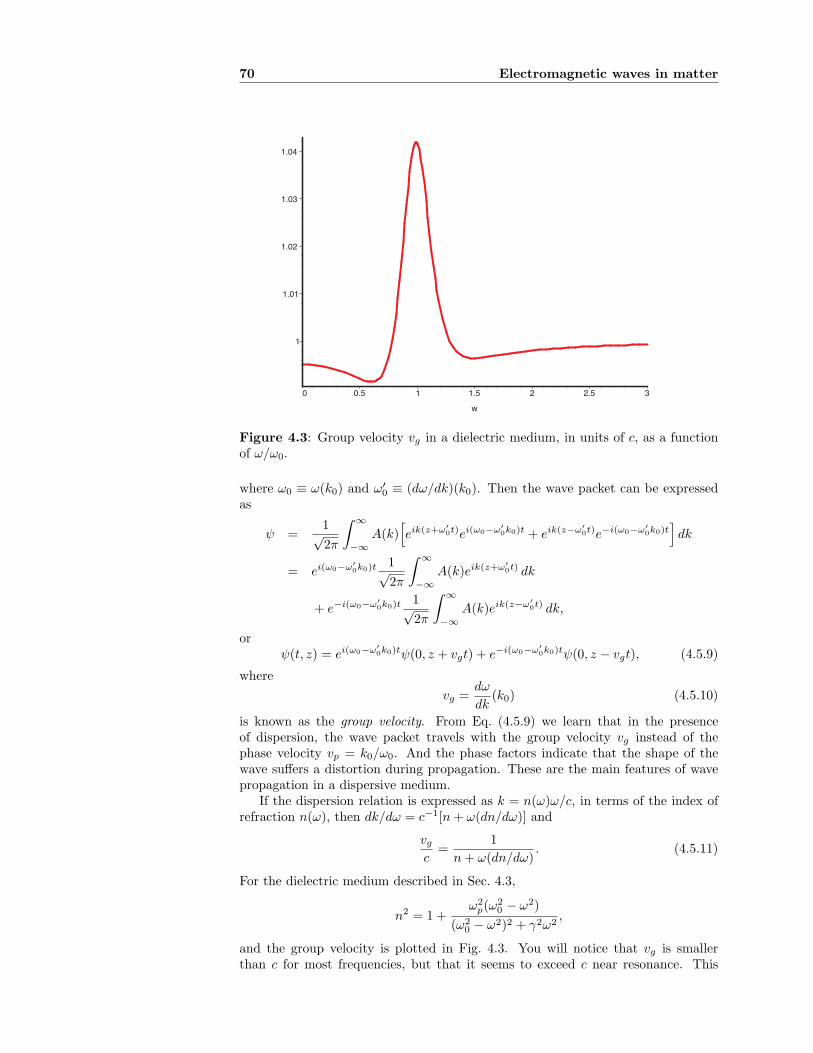
70 Electromagnetic waves in matter
1
1.01
1.02
1.03
1.04
0 0.5 1 1.5 2 2.5 3
w
Figure 4.3: Group velocity vg in a dielectric medium, in units of c, as a functionof ω/ω0.
where ω0 ≡ ω(k0) and ω′0 ≡ (dω/dk)(k0). Then the wave packet can be expressed
as
ψ =1√2π
! ∞
−∞A(k)
1
eik(z+ω′
0t)ei(ω0−ω′
0k0)t + eik(z−ω′
0t)e−i(ω0−ω′
0k0)t
2
dk
= ei(ω0−ω′
0k0)t 1√
2π
! ∞
−∞A(k)eik(z+ω′
0t) dk
+ e−i(ω0−ω′
0k0)t 1√
2π
! ∞
−∞A(k)eik(z−ω′
0t) dk,
orψ(t, z) = ei(ω0−ω′
0k0)tψ(0, z + vgt) + e−i(ω0−ω′
0k0)tψ(0, z − vgt), (4.5.9)
where
vg =dω
dk(k0) (4.5.10)
is known as the group velocity. From Eq. (4.5.9) we learn that in the presenceof dispersion, the wave packet travels with the group velocity vg instead of thephase velocity vp = k0/ω0. And the phase factors indicate that the shape of thewave suffers a distortion during propagation. These are the main features of wavepropagation in a dispersive medium.
If the dispersion relation is expressed as k = n(ω)ω/c, in terms of the index ofrefraction n(ω), then dk/dω = c−1[n + ω(dn/dω)] and
vg
c=
1
n + ω(dn/dω). (4.5.11)
For the dielectric medium described in Sec. 4.3,
n2 = 1 +ω2
p(ω20 − ω2)
(ω20 − ω2)2 + γ2ω2
,
and the group velocity is plotted in Fig. 4.3. You will notice that vg is smallerthan c for most frequencies, but that it seems to exceed c near resonance. This
4.5 Propagation of wave packets 71
phenomenon is entirely artificial: when ω is close to ω0 it is no longer true that ωis a slowly varying function of k, and the approximations involved in defining thegroup velocity are no longer valid. Furthermore, the imaginary part of ω, togetherwith the dissipative effects it represents, cannot be neglected near resonance. Thebottom line is that the very notion of group velocity is no longer meaningful near aresonance.
4.5.4 Gaussian wave packet
As a concrete example of wave propagation with dispersion we consider an initialconfiguration given by
ψ(0, z) = e−z2/(2L2) cos(k0z); (4.5.12)
this is an oscillating wave (with wave number k0) modulated by a Gaussian envelopeof width L. Once more we take the initial data to be time-symmetric, and weimpose ψ(0, z) = 0. In order to be able to carry out the calculations we shall takethe dispersion relation to be
ω(k) = ν
"
1 +1
2α2k2
#
, (4.5.13)
where ν is a minimum frequency and α an arbitrary length scale. This dispersionrelation is not particularly realistic, but its quadratic form will allow us to evaluatethe integrals that will appear in the course of our analysis. These will have the formof Gaussian integrals, and we quote the standard result
! ∞
−∞e−az2+bz+c dz =
5
π
aexp
"
b2
4a+ c
#
. (4.5.14)
Here the constants a, b, and c can be complex, but Re(a) must be positive for theintegral to converge.
We first calculate the Fourier amplitudes associated with Eq. (4.5.12). Equation(4.5.5) gives
A(k) =1
2
1√2π
! ∞
−∞ψ(0, z)e−ikz dz
=1
4
1√2π
! ∞
−∞e−z2/(2L2)
1
e−i(k−k0)z + e−i(k+k0)z2
dz.
For the first integral we have a = 1/(2L2), b = −i(k − k0), c = 0, and b2/(4a) =− 1
2 (k − k0)2L2; for the second integral we simply make the substitution k0 → −k0
in this result. Equation (4.5.14) then gives
A(k) =L
4
1
e−1
2(k−k0)
2L2
+ e−1
2(k+k0)
2L22
. (4.5.15)
We see that A(k) is a symmetric function of k, and that it is peaked at both k = k0
and k = −k0. The width of the distribution around both peaks is equal to 1/L.The wave packet at times t = 0 is given by Eq. (4.5.2),
ψ =1√2π
! ∞
−∞A(k)ei[kz−ω(k)t] dk +
1√2π
! ∞
−∞A(k)ei[kz+ω(k)t] dk,
which we may also express as
ψ =1√2π
! ∞
−∞A(k)ei[kz−ω(k)t] dk +
1√2π
! ∞
−∞A(−k)e−i[kz−ω(−k)t] dk,
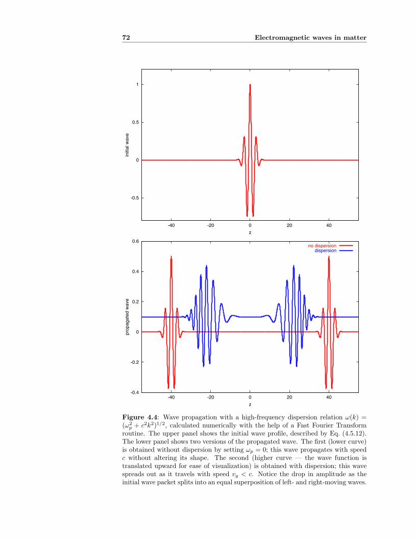
72 Electromagnetic waves in matter
-0.5
0
0.5
1
-40 -20 0 20 40
initi
al w
ave
z
-0.4
-0.2
0
0.2
0.4
0.6
-40 -20 0 20 40
prop
agat
ed w
ave
z
no dispersiondispersion
Figure 4.4: Wave propagation with a high-frequency dispersion relation ω(k) =(ω2
p + c2k2)1/2, calculated numerically with the help of a Fast Fourier Transformroutine. The upper panel shows the initial wave profile, described by Eq. (4.5.12).The lower panel shows two versions of the propagated wave. The first (lower curve)is obtained without dispersion by setting ωp = 0; this wave propagates with speedc without altering its shape. The second (higher curve — the wave function istranslated upward for ease of visualization) is obtained with dispersion; this wavespreads out as it travels with speed vg < c. Notice the drop in amplitude as theinitial wave packet splits into an equal superposition of left- and right-moving waves.
4.6 Problems 73
having changed the variable of integration to −k in the second integral. BecauseA(−k) = A(k) and ω(−k) = ω(k), we have
ψ =1√2π
! ∞
−∞A(k)ei[kz−ω(k)t] dk + complex conjugate,
=2√2π
Re
! ∞
−∞A(k)ei[kz−ω(k)t] dk.
Substituting Eq. (4.5.15) then gives
ψ =L
2√
2πRe
8! ∞
−∞e−
1
2(k−k0)
2L2
ei[kz−ω(k)t] dk + (k0 → −k0)
9
.
Taking into account Eq. (4.5.13), we see that the argument of the exponentialfunction is a second-order polynomial in k, which we write as −ak2 + bk + c, witha = 1
2 (L2 + iνtα2), b = k0L2 + iz, and c = −(iνt + 12k2
0L2). With this we have
b2
4a= −
(z − ik0L2)2
2L2(1 + iνtf2),
where f ≡ α/L, and Eq. (4.5.14) yields
ψ =1
2Re
8
(1 + iνtf2)−1/2exp
3
−(z − ik0L2)2
2L2(1 + iνtf2)
4
e−iνt− 1
2k2
0L2
+ (k0 → −k0)
9
.
It is then a matter of straightforward algebra to bring this to its final form,
ψ(t, z) =1
2Re
8
(1 + iνtf2)−1/2exp
3
−(z − vgt)2
2L2(1 + iνtf2)
4
ei[k0z−ω(k0)t]
+ (k0 → −k0)
9
, (4.5.16)
where f = α/L and
vg = να2k0 =dω
dk(k0) (4.5.17)
is the group velocity at k = k0 for the dispersion relation of Eq. (4.5.13).Equation (4.5.16) informs us that the wave packet retains its Gaussian shape as
it propagates through the medium, but that its width increases with time:
L(t) = L0
1 + (f2νt)2. (4.5.18)
The wave therefore spreads out, and this is a typical feature of propagation withdispersion. In addition, we see that while the oscillations travel at the phase velocityvp = ω(k0)/k0, the centre of the Gaussian peak travels at the group velocity vg;this result was expected after the discussion of the preceding subsection.
A more realistic example of wave dispersion (calculated numerically) is displayedin Fig. 4.4. Notice that the features discussed in the preceding paragraphs arepresent in this example as well: the wave packet spreads out as it propagates witha group velocity vg that is smaller than c.
4.6 Problems
1. (This problem is adapted from Jackson’s problem 7.19.) A wave packet inone dimension has an initial shape given by ψ(0, z) = f(z)eik0z, where f(z) isthe modulation envelope; the wave packet is assumed to be time-symmetric.For each of the forms f(z) given below, calculate the wave-number spec-trum |A(k)|2 of the wave packet, sketch |ψ(0, z)|2 and |A(k)|2, calculate theroot-mean-square deviations ∆z and ∆k from the means (defined in terms of|ψ(0, z)|2 and |A(k)|2, respectively), and test the inequality ∆z∆k ≥ 1
2 .
74 Electromagnetic waves in matter
a) f(z) = e−α|z|/2;
b) f(z) = e−α2z2/4;
c) f(z) = 1 − α|z| for α|z| < 1 and f(z) = 0 for α|z| > 1;
d) f(z) = 1 for α|z| < 1 and f(z) = 0 for α|z| > 1.
2. We have seen that the relationship between the frequency-domain fields Dand E is
D(ω,x) = ϵ(ω)E(ω,x),
whereϵ(ω)
ϵ0= 1 +
ω2p
ω20 − ω2 − iγω
.
Prove that as a consequence of this, the relationship between the time-domainfields D and E is
D(t,x) = ϵ0
3
E(t,x) +ω2
p
ν
! ∞
0e−γτ/2 sin(ντ)E(t − τ,x) dτ
4
,
where ν ≡A
ω20 − 1
4γ2. This reveals that D at time t depends on the electric
field at all previous times: the relationship is nonlocal in time. The exponen-tial factor, however, indicates that delays longer than 1/γ do not matter verymuch: only the electric field’s recent history is important.
Chapter 5
Electromagnetic radiation
from slowly moving sources
5.1 Equations of electrodynamics
In this chapter and the next we will explore some of the mechanisms by whichelectromagnetic radiation is produced. While Chapter 6 will be concerned withrelativistic situations, here we shall restrict our attention to charge and currentdistributions whose internal velocities are small compared with the speed of light.
We recall the main equations of electrodynamics, as we have formulated themin Chapter 1. We have wave equations for the scalar and vector potentials,
!Φ(t,x) = −1
ϵ0ρ(t,x) (5.1.1)
and!A(t,x) = −µ0j(t,x), (5.1.2)
where
! ≡ −1
c2
∂2
∂t2+ ∇2 (5.1.3)
is the wave operator and c ≡ (ϵ0µ0)−1/2 is the speed of light. For Eqs. (5.1.1)and (5.1.2) to be equivalent to Maxwell’s equations, the potentials must satisfy theLorenz gauge condition,
∇ · A +1
c2
∂Φ
∂t= 0. (5.1.4)
Maxwell’s equations imply that the charge and current densities satisfy the conti-nuity equation,
∂ρ
∂t+ ∇ · j = 0, (5.1.5)
which states that charge is locally conserved.In the absence of boundaries, the wave equations have solutions
Φ(t,x) =1
4πϵ0
!
ρ(t − |x − x′|/c,x′)
|x − x′|d3x′ (5.1.6)
and
A(t,x) =µ0
4π
!
j(t − |x − x′|/c,x′)
|x − x′|d3x′; (5.1.7)
these are retarded solutions, which incorporate the physically appropriate causalrelationship between sources and fields.
75
76 Electromagnetic radiation from slowly moving sources
From the potentials we obtain the fields via the relations
E = −∂A
∂t− ∇Φ (5.1.8)
andB = ∇ × A. (5.1.9)
And finally, we recall from Sec. 1.4 that the fields carry energy. The electromagneticfield energy density is given by
ε(t,x) =1
2ϵ0E
2 +1
2µ0B2 (5.1.10)
and the energy flux vector (Poynting vector) is
S(t,x) =1
µ0E × B. (5.1.11)
5.2 Plane waves
The simplest situation featuring the production of electromagnetic waves involvesmonochromatic plane waves. These are generated by a planar distribution ofcharges, all oscillating in the plane with the same frequency ω.
We take the charge distribution to be uniform in the x-y plane, so that thecharge density is given by
ρ(t,x) = σδ(z), (5.2.1)
where σ is a constant surface density. Notice that the charge density is actuallytime independent. The resulting scalar potential will also not depend on time, andthe electromagnetic waves will be described entirely by the vector potential.
We take each charge to be oscillating in the x direction with a velocity
v(t,x) = v0x cos ωt. (5.2.2)
Notice that the velocity vector is actually independent of position in the plane, andthat x is actually an arbitrary direction within the plane; we could pick anotherdirection by rotating the x-y coordinates around the z axis. The current density is
j(t,x) = σv0δ(z)x cos ωt, (5.2.3)
and we will calculate the associated vector potential without approximations.In principle we might proceed by substituting Eq. (5.2.3) into Eq. (5.1.7), but
it is easier to start instead with the equivalent form
A(t,x) =µ0
4π
!
j(t′,x′)δ(t − t′ − |x − x′|/c)
|x − x′|dt′d3x′,
in which we substitute Eq. (5.2.3) expressed in terms of primed variables. We have
A(t,x) =µ0
4πσv0x
!
dt′ Γ(t − t′,x) cos ωt′,
where
Γ(t − t′,x) =
!
δ(z′)δ(t − t′ − |x − x′|/c)
|x − x′|d3x′
is an integral that we must now evaluate.
5.2 Plane waves 77
Integration over dz′ is immediate:
Γ =
!
δ(t − t′ −0
(x − x′)2 + (y − y′)2 + z2/c)0
(x − x′)2 + (y − y′)2 + z2dx′dy′,
or
Γ =
!
δ(t − t′ −0
x′2 + y′2 + z2/c)0
x′2 + y′2 + z2dx′dy′
after translating the origin of the (x′, y′) coordinates to the point (x, y); this isallowed, because the domain of integration is the whole x′-y′ plane. To integratethis we make the change of variables x′ = ℓ cos θ, y′ = ℓ sin θ. This gives, afterwriting dx′dy′ = ℓ dℓdθ and integrating over dθ,
Γ = 2π
! ∞
0
δ(t − t′ −√
ℓ2 + z2/c)√ℓ2 + z2
ℓ dℓ.
The easiest way to integrate over the δ-function is to make its argument be theintegration variable. So let s =
√ℓ2 + z2/c − ∆t, where ∆t ≡ t − t′. Because ℓ is
nonnegative, we have that s is bounded below by |z|/c − ∆t. We also have
ds =ℓ dℓ
c√
ℓ2 + z2=
ℓ dℓ
c2(s + ∆t),
and the integral becomes
Γ = 2πc
! ∞
|z|/c−∆tδ(s) ds,
orΓ(t − t′,x) = 2πcθ(t − t′ − |z|/c),
where θ(s) is the step function, which is unity when s > 0 and zero otherwise.Substituting this result into our previous expression for the vector potential, we
obtain
A(t,x) =µ0
4π(σv0)(2πc)x
! ∞
−∞dt′ θ(t − |z|/c − t′) cos ωt′
=µ0
4π2πσv0c x
! t−|z|/c
−∞cos ωt′ dt′.
The dt′ integral evaluates to ω−1 sin ω(t− |z|/c), apart from an ambiguous constantassociated with the integral’s infinite lower bound. Since this constant will neverappear in expressions for the electric and magnetic fields, we simply set it to zero.Our final expression for the vector potential is therefore
A(t, z) =E0
ωsin ω(t − |z|/c)x, (5.2.4)
where
E0 =1
2µ0σv0c (5.2.5)
has the dimensions of an electric field. For z > 0 we have that sinω(t − |z|/c) =sin ω(t − z/c) = − sin k(z − ct), where k = ω/c is the wave number, and we seethat the wave travels in the positive z direction with speed c. For z < 0 we haveinstead sin ω(t− |z|/c) = sin ω(t + z/c) = sin k(z + ct), and the wave now travels inthe negative z direction. Thus, Eq. (5.2.4) describes a plane wave that propagatesaway from z = 0, the place where it is generated; the wave has a frequency ω, awave number k = ω/c, and it travels with the speed of light.
78 Electromagnetic radiation from slowly moving sources
The time-dependent part of the electric field is obtained from Eqs. (5.1.8) and(5.2.4):
E(t, z) = −E0 cos ω(t − |z|/c)x. (5.2.6)
We see that the electric field behaves as a plane wave that travels away from z = 0with the speed of light, and that it points in the x direction, which is perpendicularto the direction of propagation. The magnetic field, on the other hand, is obtainedby taking the curl of Eq. (5.2.4). This involves differentiating |z| with respect to z,which is +1 for z > 0 and −1 if z < 0. Denoting this function by ϵ(z) ≡ θ(z)−θ(−z),we have
B(t, z) =E0
cϵ(z) cos ω(t − |z|/c)y. (5.2.7)
The magnetic field also is a plane wave that travels away from z = 0 at the speed oflight, and it points in the y direction, which is perpendicular to both the directionof propagation and the direction of the electric field. Notice that E and B areboth proportional to cosω(t − |z|/c): the fields are in phase. Notice also that |B|is smaller than |E| by a factor 1/c.
To finish off our discussion of plane electromagnetic waves, we calculate thefield’s energy density and flux vector. From Eqs. (5.1.10), (5.2.6), and (5.6.7) weobtain
ε(t, z) = ϵ0E20 cos2 ω(t − |z|/c), (5.2.8)
and from Eq. (5.1.11) we get
S(t, z) = cϵ(z)ε(t, z)z. (5.2.9)
This shows that the electromagnetic field energy travels with the wave, in the pos-itive or negative z direction, away from the source, and with the speed of light.
Let us summarize the main points:
• The plane wave travels in the (positive or negative) z direction with speed c.
• The electric and magnetic fields are perpendicular to z and to each other.
• The fields are in phase.
• Their magnitudes are related by |B|/|E| = 1/c.
• The electromagnetic field energy travels with the wave.
These properties are generic: they are shared by all electromagnetic waves. Theonly caveat is that in general, the direction of propagation is not uniform: theconstant vector z goes into a vector n that may change from point to point.
5.3 Spherical waves — the oscillating dipole
[The material presented in this section is also covered in Secs. 9.1 and 9.2 of Jack-son’s text.]
5.3.1 Plane versus spherical waves
Any function of the formψ(t, z) = f(t ∓ z/c), (5.3.1)
where f(ξ) is an arbitrary function of ξ = t∓z/c, is a solution to the wave equation!ψ = 0. If ξ = t−z/c, the plane wave travels in the positive z direction with speedc; if instead ξ = t + z/c, the wave travels in the negative z direction. To see thatEq. (5.3.1) does indeed form a valid solution to the wave equation, we note that
5.3 Spherical waves — the oscillating dipole 79
∂ψ/∂t = f ′(ξ) while ∂ψ/∂z = ∓f ′(ξ)/c, where a prime indicates differentiation withrespect to ξ; substitution into the wave operator yields !ψ = −c−2f ′′ + c−2f ′′ = 0,as required.
Plane waves are not a very good approximation to realistic waves, which orig-inate in a localized region of space and propagate outward with a decreasing am-plitude. A better approximation that incorporates these features is the sphericalwave
ψ(t, r) =1
rf(t − r/c), (5.3.2)
where f(u) is an arbitrary function of u = t−r/c. This is also a solution to !ψ = 0.Here the wavefronts are spherical instead of planar, and the wave propagates out-ward in the radial direction; its amplitude decays as 1/r, giving rise to an intensitythat goes as 1/r2. That Eq. (5.3.2) forms a valid solution to the wave equationfollows by direct substitution: In the absence of an angular dependence the waveoperator reduces to
! = −1
c2
∂2
∂t2+
1
r2
∂
∂rr2 ∂
∂r.
Differentiating with respect to t yields ∂2ψ/∂t2 = r−1f , while we have r2∂ψ/∂r =−rf/c − f and
∂
∂rr2 ∂ψ
∂r= −
1
cf +
1
c2rf +
1
cf =
1
c2rf ,
where an overdot indicates differentiation with respect to u. All this gives !ψ = 0,as required. Note that a similar calculation would reveal that ψ = r−1f(t + r/c)also is a solution to the wave equation; this wave travels inward instead of outward.
5.3.2 Potentials of an oscillating dipole
The simplest electromagnetic spherical wave is produced by an oscillating dipolelocated at the origin of the coordinate system. Here and in the following subsectionswe will calculate the potentials and fields produced by this dipole, and examine thenature of the corresponding electromagnetic radiation.
In Sec. 2.3 we saw that the charge density of a point dipole could be expressed asρ(x) = −p·∇δ(x), where p was a constant dipole moment vector. Here we introducea time dependence by making p oscillate with angular frequency ω: p → p cos ωt.The charge density of an oscillating dipole is then
ρ(t,x) = −p · ∇δ(x) cos ωt. (5.3.3)
Notice that in this equation, p is still a constant vector, which we align with the zaxis: p = pz.
A time-varying charge density must be associated with a current density j,because
∇ · j = −∂ρ
∂t= −ωp · ∇δ(x) sin ωt = ∇ ·
'
−ωpδ(x) sin ωt(
.
The simplest solution to this equation is
j(t,x) = −ωpδ(x) sin ωt, (5.3.4)
and this is the current density of an oscillating dipole.We first compute the vector potential produced by the current density of Eq. (5.3.4).
Once more it is convenient to start with the expression
A(t,x) =µ0
4π
!
j(t′,x′)δ(t − t′ − |x − x′|/c)
|x − x′|dt′d3x′.
80 Electromagnetic radiation from slowly moving sources
After substituting Eq. (5.3.5) we obtain
A(t,x) = −µ0
4πωp
!
dt′ sin ωt′!
δ(x′)δ(t − t′ − |x − x′|/c)
|x − x′|d3x′
= −µ0
4πωp
!
dt′ sin ωt′δ(t − t′ − r/c)
r,
or
A(t,x) = −µ0
4πωp
sinω(t − r/c)
r. (5.3.5)
This has the structure of a spherical wave, with its expected dependence on u =t − r/c and its amplitude decaying as 1/r.
We may now compute the scalar potential. This calculation is a bit more labo-rious, and we start with
Φ(t,x) =1
4πϵ0
!
ρ(t′,x′)δ(t − t′ − |x − x′|/c)
|x − x′|dt′d3x′.
After substituting Eq. (5.3.3) we get
Φ(t,x) = −1
4πϵ0p ·
!
dt′Γ(t − t′,x) cos ωt′,
where
Γ(t − t′,x) =
!
'
∇′δ(x′)
(δ(t − t′ − |x − x′|/c)
|x − x′|d3x′
is a vectorial integral that we must now evaluate.Integration by parts allows us to write
Γ = −!
δ(x′)∇′
3
δ(t − t′ − |x − x′|/c)
|x − x′|
4
d3x′.
Because the dependence on x′ is contained entirely in |x−x′|, and because ∇′|x−x′| = −(x − x′)/|x − x′|, evaluating the gradient gives
Γ = −!
δ(x′)
3
δ(t − t′ − |x − x′|/c)
|x − x′|2+
1
c
δ′(t − t′ − |x − x′|/c)
|x − x′|
4
x − x′
|x − x′|d3x′
= −3
δ(t − t′ − r/c)
r2+
1
c
δ′(t − t′ − r/c)
r
4
x
r,
or
Γ(t − t′,x) = −r
3
δ(t − t′ − r/c)
r2+
1
c
δ′(t − t′ − r/c)
r
4
,
where r = x/r.Substituting this result into our previous expression for the scalar potential, we
obtain
Φ(t,x) =1
4πϵ0p · r
!
dt′3
δ(t − t′ − r/c)
r2+
1
c
δ′(t − t′ − r/c)
r
4
cos ωt′,
and integrating against the δ-functions gives
Φ(t,x) =1
4πϵ0p · r
3
cos ω(t − r/c)
r2−
ω
c
sinω(t − r/c)
r
4
.
One must be careful with the second term: a minus sign comes from the integrationby part needed to convert δ′(t − t′ − r/c) into an actual δ-function, but this minus
5.3 Spherical waves — the oscillating dipole 81
sign is canceled out because the prime on the δ-function indicates differentiationwith respect to t − t′ − r/c instead of t′. We express our final result as
Φ = Φnear + Φwave, (5.3.6)
where
Φnear(t,x) =1
4πϵ0
p · rr2
cos(ωu) (5.3.7)
and
Φwave(t,x) = −1
4πϵ0
ω
cp · r
sin(ωu)
r, (5.3.8)
and where u = t − r/c is retarded time.The scalar potential contains two terms. Of these, only Φwave has the mathe-
matical structure of a spherical wave. The other term, Φnear, has the structure of astatic dipole field,
Φdipole(x) =1
4πϵ0
p · rr2
,
to which a time dependence cos(ωu) is attached. Unlike Φwave, this term does notrepresent electromagnetic radiation. Instead, Φnear describes the field of a pointdipole, and this field follows the dipole’s time dependence with the usual delay: thecos ωt dependence of the dipole is replaced by cosω(t − r/c).
As the name indicates, Φnear dominates when r is small, while Φwave dominateswhen r is large. The scalar potential becomes purely radiative when r is sufficientlylarge that Φnear can be neglected; the region of space for which this is true is calledthe wave zone. On the other hand, the region of space for which r is sufficientlysmall that Φwave can be neglected in front of Φnear is called the near zone.
In the near zone we must have 1/r2 ≫ ω/(cr), or
r ≪c
ω=
1
k=
λ
2π(near zone), (5.3.9)
where k is the wave number and λ the wavelength. In the near zone, u = t−r/c ≃ tand the delay contained in the retarded time is hardly noticeable — the near-zonefield responds virtually instantaneously to changes in the source. In the wave zonewe have instead 1/r2 ≪ ω/(cr), or
r ≫c
ω=
1
k=
λ
2π(wave zone). (5.3.10)
Here the time delay is important, and the scalar potential behaves as a true sphericalwave. In the region of space where r is comparable to c/ω, between the near zoneand the wave zone (a region that is sometimes called the induction, or intermediate,zone), Φnear and Φwave are comparable, and the scalar potential behaves neither asan instantaneously-changing dipole field nor as a spherical wave.
5.3.3 Wave-zone fields of an oscillating dipole
Let us calculate the electric and magnetic fields in the wave zone. We use theexpressions
A(t,x) = −µ0
4πωp
sin(ωu)
r(5.3.11)
and
Φ(t,x) = −1
4πϵ0
ω
cp · r
sin(ωu)
r, (5.3.12)
where u = t − r/c is retarded time. Notice that Eq. (5.3.11) is exact, whileEq. (5.3.12) is valid in the wave zone only.
82 Electromagnetic radiation from slowly moving sources
To do this calculation we will need to compute the gradient of
ψ(t, r) ≡sin(ωu)
r.
We have ∇ψ = (∂ψ/∂r)∇r = (∂ψ/∂r)r and
∂ψ
∂r= −
sin(ωu)
r2−
ω
c
cos(ωu)
r,
because ∂u/∂r = 1/c. But since we are working in the wave zone, the first termcan be neglected and we obtain the useful approximation
∇sin(ωu)
r= −
ω
c
cos(ωu)
rr. (5.3.13)
We might also need the gradient of p · r. To see what this is, consider its x compo-nent:
∇x
"
p ·x
r
#
= −p · xr2
x
r+
px
r,
so that
∇(p · r) =p − (p · r)r
r. (5.3.14)
The fact that this is of order 1/r means that the gradient of p · r will be negligiblein our forthcoming calculations.
The electric field is related to the potentials by Eq. (5.1.8),
E = −∂A
∂t− ∇Φ.
Substituting Eqs. (5.3.11) and (5.3.12), we obtain
E =µ0
4πω2p
cos(ωu)
r+
1
4πϵ0
ω
c
3
sin(ωu)
r∇(p · r) + (p · r)∇
sin(ωu)
r
4
.
Using Eq. (5.3.14) shows that the first term within the square brackets is of order1/r2 and can be neglected in the wave zone, while using Eq. (5.3.13) gives
E =µ0
4πω2p
cos(ωu)
r−
1
4πϵ0
ω2
c2(p · r)
cos(ωu)
rr.
Collecting the terms and recalling that ϵ0µ0 = 1/c2 brings this to its final form
Ewave(t,x) =µ0
4πω2
'
p − (p · r)r(cos(ωu)
r. (5.3.15)
This has the structure of a spherical wave, and we notice that Ewave is transverseto the direction in which the wave propagates:
Ewave · r = 0. (5.3.16)
If, for concreteness, we let p point in the z direction, then p = pz, r = sin θ cos φx+sin θ sin φy + cos θz, p · r = p cos θ, and p − (p · r)r = −p sin θ(cos θ cos φx +cos θ sin φy−sin θz) = −p sin θθ, where θ is a unit vector that points in the directionof increasing θ. This yields
Ewave(t,x) = −µ0
4πω2p sin θ
cos(ωu)
rθ (5.3.17)
for the electric field.
5.3 Spherical waves — the oscillating dipole 83
The magnetic field is obtained by taking the curl of the vector potential. Wehave
B(t,x) =µ0
4πωp × ∇
sin(ωu)
r,
and Eq. (5.3.13) gives us
Bwave(t,x) =µ0
4π
ω2
c(r × p)
cos(ωu)
r. (5.3.18)
The magnetic field also is a spherical wave, and like the electric field it is transverseto the direction of propagation:
Bwave · r = 0. (5.3.19)
Furthermore, we see from Eqs. (5.3.15) and (5.3.18) that the fields are mutuallyorthogonal, because [p− (p · r)r] · (r×p) = p · (r×p)− (p · r)r · (r×p) = 0, sincethe vector r × p is perpendicular to both p and r. So the fields satisfy
Ewave · Bwave = 0 (5.3.20)
in the wave zone. For p = pz we have r × p = −p sin θ(− sin φx + cos φy) =−p sin θφ, and Eq. (5.3.18) becomes
Bwave(t,x) = −µ0
4π
ω2
cp sin θ
cos(ωu)
rφ. (5.3.21)
5.3.4 Poynting vector of an oscillating dipole
We now calculate S = µ−10 E × B, the energy flux vector associated with the
electromagnetic radiation produced by the oscillating dipole. It is easy to checkthat in the wave zone, the electric and magnetic fields are related by
Ewave = cBwave × r. (5.3.22)
This follows because the magnetic field is proportional to r × p, and (r × p)× r =(r · r)p− (r ·p)r = p− (p · r)r, which gives the direction of the electric field. Usingonce more the same vectorial identity, the Poynting vector is
S =c
µ0
%
B × r&
× B =c
µ0
1
(B · B)r − (B · r)B2
.
The second term vanishes because B is orthogonal to r, and we arrive at
Swave(t,x) =c
µ0
+
+Bwave(t,x)+
+
2r. (5.3.23)
This shows that the energy is transported in the radial direction, the same directionin which the wave propagates.
For p = pz we can substitute Eq. (5.3.21) into Eq. (5.3.23) and obtain
S =c
µ0
"
µ0
4π
#2 ω4p2 sin2 θ
c2
cos2(ωu)
r2r
=µ0p2ω4
16π2c
sin2 θ
r2cos2(ωu) r.
The energy flux oscillates in time, and after averaging over a complete wave cyclewe get
⟨Swave⟩ =µ0p2ω4
32π2c
sin2 θ
r2r. (5.3.24)
84 Electromagnetic radiation from slowly moving sources
From the angular dependence of this expression we see that most of the energy isemitted near the equatorial plane (θ = π
2 ), and that none of the energy propagatesalong the z axis (θ = 0 or θ = π). The average of any function f of retarded time u
over a complete wave cycle is defined by ⟨f(u)⟩ ≡ T−1* T0 f(u) du, where T = 2π/ω
is the oscillation period. Using this rule we get ⟨cos2(ωu)⟩ = 12 , and this gives
Eq. (5.3.24).The total power radiated (energy per unit time) is obtained by integrating S
(energy per unit time per unit area) over any closed surface S. The averaged poweris then
⟨P ⟩ =
)
S⟨S⟩ · da. (5.3.25)
It is simplest to take S to be a sphere of constant r. Then da = rr2 sin θ dθdφ, andEq. (5.3.25) becomes
⟨P ⟩ =µ0p2ω4
32π2c2π
! π
0sin3 θ dθ.
The integral evaluates to 4/3, and we obtain
⟨P ⟩ =µ0
12πcp2ω4. (5.3.26)
5.3.5 Summary — oscillating dipole
We have seen that in the wave zone (r ≫ c/ω), the fields of an oscillating dipoleare given by
E(t, r, θ,φ) = −µ0
4πω2p sin θ
cos ω(t − r/c)
rθ
and
B(t, r, θ,φ) = −µ0
4π
ω2
cp sin θ
cos ω(t − r/c)
rφ.
These have the structure of a spherical wave, which travels outward at the speed oflight. They are produced by a charge distribution whose dipole moment vector isgiven by p(t) = p cos(ωt)z. The field amplitudes are related by |B|/|E| = 1/c, andboth fields are in phase. The electric field is directed along
θ = cos θ cos φ x + cos θ sin φ y − sin θ z
while the magnetic field is directed along
φ = − sin φ x + cos φ y.
The fields are mutually orthogonal, and they are both transverse to
r = sin θ cos φ x + sin θ sinφ y + cos θ z,
the direction in which the wave is traveling. This is also the direction in whichthe field energy is transported. The angular profile of the energy-flux (Poynting)vector is described by sin2 θ, so that most of the energy is emitted in the directionsorthogonal to the dipole.
5.4 Electric dipole radiation
[The material presented in this section is also covered in Sec. 9.2 of Jackson’s text.]We now consider a much more general situation, in which electromagnetic ra-
diation is produced by an arbitrary distribution of charges and currents, with anarbitrary time dependence (not necessarily oscillating with a single frequency ω).Our only restrictions are that
5.4 Electric dipole radiation 85
• the source is confined to a bounded region V of space;
• the charges are moving slowly.
These conditions will allow us to formulate useful approximations for the behaviourof the electric and magnetic fields. Although the present context is very general, wewill see that the results to be derived in this section are very close to those obtainedin the preceding section.
5.4.1 Slow-motion approximation; near and wave zones
To make the slow-motion approximation precise, and to define near and wave zonesin the general case, we introduce the following scaling quantities:
rc ≡ characteristic length scale of the charge and current distribution,
tc ≡ characteristic time scale over which the distribution changes,
vc ≡rc
tc≡ characteristic velocity of the source,
ωc ≡2π
tc≡ characteristic frequency of the source,
λc ≡2πc
ωc≡ ctc ≡ characteristic wavelength of the radiation.
The characteristic length scale is defined such that if ρ(t,x′) and j(t,x′) are thecharge and current densities, respectively, then |x′| is at most of order rc throughoutthe source. This implies that the distribution of charge and current is localizedwithin a region whose volume is of the order of r3
c . The characteristic time scale isdefined such that ∂ρ/∂t is of order ρ/tc throughout the source. If, for example, ρoscillates with a frequency Ω, then tc ∼ 1/Ω and ωc ∼ Ω.
The slow-motion approximation means that vc = rc/tc is much smaller than thespeed of light:
vc ≪ c. (5.4.1)
This condition gives us rc = vctc ≪ ctc = λc, or
rc ≪ λc. (5.4.2)
The source is therefore confined to a region that is much smaller than a typicalwavelength of the radiation.
We can now define the near and wave zones:
near zone: |x − x′| ≪λc
2π=
c
ωc, (5.4.3)
wave zone: |x − x′| ≫λc
2π=
c
ωc. (5.4.4)
Because rc ≪ λc, the wave zone can also be defined by the condition r ≫ λc/(2π).We will compute the potentials and fields in these zones, using Eqs. (5.4.1)–(5.4.4)to simplify our expressions.
5.4.2 Scalar potential
We begin by calculating the scalar potential,
Φ(t,x) =1
4πϵ0
!
V
ρ(t − |x − x′|/c,x′)
|x − x′|d3x′,
86 Electromagnetic radiation from slowly moving sources
where V is the region of space occupied by the source. In the near zone we cantreat |x−x′|/c as a small quantity and Taylor-expand the charge density about thecurrent time t. Because ρ(t − ε) = ρ(t) − ρ(t)ε + 1
2 ρ(t)ε2 + · · · we have
ρ(t − |x − x′|/c) = ρ(t) −1
cρ(t)|x − x′| + · · · ,
where an overdot indicates differentiation with respect to t. Relative to the firstterm, the second term is of order |x − x′|/(ctc) = |x − x′|/λc, and by virtue ofEq. (5.4.3), this is small in the near zone. The third term would be smaller still,and we neglect it. We then have
Φ(t,x) =1
4πϵ0
3!
V
ρ(t,x′)
|x − x′|d3x′ −
1
c
!
ρ(t,x′) d3x′ + · · ·4
=1
4πϵ0
3!
V
ρ(t,x′)
|x − x′|d3x′ −
1
c
d
dt
!
Vρ(t,x′) d3x′ + · · ·
4
.
The second term vanishes, because it involves the time derivative of the total charge*
ρ(t,x′) d3x′, which is conserved. We have obtained
Φnear(t,x) =1
4πϵ0
!
V
ρ(t,x′)
|x − x′|
3
1 + O
"
|x − x′|2
λ2c
#4
d3x′. (5.4.5)
We see that the near-zone potential takes its usual static expression, except for thesmall correction of order |x − x′|2/λ2
c and the fact that charge density depends ontime. The time delay between the source and the potential has disappeared, andwhat we have is a potential that adjusts instantaneously to the changes within thedistribution. The electric field it produces is then a “time-changing electrostaticfield”. This near-zone field does not behave as radiation.
To witness radiative effects we must go to the wave zone. Here |x− x′| is largeand we can no longer Taylor-expand the density as we did previously. Instead wemust introduce another approximation technique. We use the fact that in the wavezone, r is much larger than r′, so that
|x − x′| =0
(x − x′) · (x − x′)
=0
r2 − 2x · x′ + r′2
= r1
1 − 2r · x′/r + O(r2c/r2)
21/2
= r1
1 − r · x′/r + O(r2c/r2)
2
= r − r · x′ + O(r2c/r).
This gives
ρ(t − |x − x′|/c) = ρ(t − r/c + r · x′/c + ϵ/c)
= ρ(u + r · x′/c + ϵ/c),
whereu = t − r/c (5.4.6)
is retarded time and ϵ is of order r2c/r. Let us now Taylor-expand the charge density
about the retarded time u instead of the current time t. We have
ρ(t − |x − x′|/c) = ρ(u) +1
cρ(u)
%
r · x′ + ϵ&
+ · · · ,
where an overdot now indicates differentiation with respect to u. We see thatrelative to r ·x′, the ϵ term is of order rc/r ≪ 1 and can be neglected. Now relative
5.4 Electric dipole radiation 87
to ρ(u), the time-derivative term is of order rc/(ctc) = vc/c, and this is small byvirtue of Eq. (5.4.1). We therefore have
ρ(t − |x − x′|/c) = ρ(u) +r · x′
cρ(u) + O
%
v2c/c2
&
(5.4.7)
in the wave zone.Inside the integral for Φ we also have
1
|x − x′|=
1
r
1
1 + r · x′/r + O(r2c/r2)
2
=1
r
1
1 + O(rc/r)2
,
and it is sufficient to keep the leading term only. The wave-zone potential is then
Φ(t,x) =1
4πϵ0
1
r
!
V
3
ρ(u) +r · x′
cρ(u) + · · ·
4
d3x′
=1
4πϵ0
1
r
3!
Vρ(u,x′) d3x′ +
r
c·
∂
∂u
!
Vρ(u,x′)x′ d3x′ + · · ·
4
.
In the first integral we recognize Q, the total charge of the distribution; this isactually independent of u by virtue of charge conservation. In the second integralwe recognize p(u), the dipole moment vector of the charge distribution; this doesdepend on retarded time u. Our final expression for the potential is therefore
Φwave(t,x) =1
4πϵ0
Q
r+
1
4πϵ0
r · p(u)
cr+ · · · , (5.4.8)
where
Q =
!
Vρ(u,x′) d3x′ (5.4.9)
is the total charge and
p(u) =
!
Vρ(u,x′)x′ d3x′ (5.4.10)
the dipole moment. The first term on the right-hand side of Eq. (5.4.8) is the static,monopole potential associated with the total charge Q. This term does not dependon time and is not associated with the propagation of radiation; we shall simplyomit it in later calculations. The second term, on the other hand, is radiative: itdepends on retarded time u = t− r/c and decays as 1/r. We see that the radiativepart of the scalar potential is produced by a time-changing dipole moment of thecharge distribution; it is nonzero whenever dp/dt is nonzero. You should check that
Φwave(t,x) ≃1
4πϵ0
r · p(u)
cr
reduces to Eq. (5.3.8) when the dipole moment is given by p(t) = p0 cos(ωt), wherep0 is a constant vector.
5.4.3 Vector potential
The exact expression for the vector potential is
A(t,x) =µ0
4π
!
V
j(t − |x − x′|/c,x′)
|x − x′|d3x′.
In the near zone we approximate the current density as
j(t − |x − x′|/c) = j(t)
3
1 + O
"
|x − x′|λc
#4
88 Electromagnetic radiation from slowly moving sources
and we obtain
Anear(t,x) =µ0
4π
!
V
j(t,x′)
|x − x′|
3
1 + O
"
|x − x′|λc
#4
d3x′. (5.4.11)
We see that here also, the vector potential takes its static form, except for thecorrection of order |x−x′|/λc and the fact that the current density depends on time.The potential responds virtually instantaneously to changes in the distribution, andthere are no radiative effects in the near zone.
In the wave zone we have instead
j(t − |x − x′|/c) = j%
u + r · x′/c&
= j(u)'
1 + O(vc/c)(
and
Awave(t,x) =µ0
4π
1
r
!
Vj(u,x′)
'
1 + O(vc/c)(
d3x′.
In static situations, the volume integral of j vanishes — recall Eq. (3.4.3). Buthere the current density depends on time, and as we shall prove presently, we haveinstead
!
Vj(u,x′) d3x′ = p(u). (5.4.12)
The vector potential is therefore
Awave(t,x) =µ0
4π
p(u)
r+ · · · (5.4.13)
in the wave zone. This has the structure of a spherical wave, and we see thatthe radiative part of the vector potential is produced by a time-changing dipolemoment. You may verify that Eq. (5.4.13) reduces to reduces to Eq. (5.3.5) whenthe dipole moment is given by p(t) = p0 cos(ωt), where p0 is a constant vector.
To establish the z component of Eq. (5.4.12) we start with the identity ∇·(zj) =z(∇ · j) + j · (∇z), in which we substitute the statement of charge conservation,∇ · j = −∂ρ/∂t. After integration over the source we have
!
Vjz d3x −
d
dt
!
Vρz d3x =
!
V∇ · (zj) d3x =
)
Szj · da,
where S is the two-dimensional surface bounding V . Because no current is crossingthis surface, the right-hand side vanishes and we have
!
Vjz d3x =
d
dt
!
Vρz d3x =
dpz
dt.
This is the same thing as the z component of Eq. (5.4.12), except for the fact thatρ and j are expressed in terms of the variables (t,x) instead of (u,x′). The othercomponents of the equation are established with similar manipulations.
5.4.4 Wave-zone fields
The potentials
Φwave(t,x) =1
4πϵ0
r · p(u)
cr
1
1 + O(vc/c)2
(5.4.14)
and
Awave(t,x) =µ0
4π
p(u)
r
1
1 + O(vc/c)2
, (5.4.15)
where u = t − r/c and r = x/r, are generated by time variations of the dipolemoment vector p of the charge and current distribution. They therefore give rise
5.4 Electric dipole radiation 89
to electric-dipole radiation, the leading-order contribution, in our slow-motion ap-proximation, to the radiation emitted by an arbitrary source. We now compute theelectric and magnetic fields in this approximation.
To get the electric field we keep only those terms that decay as 1/r, and neglectterms that decay faster. For example, when computing the gradient of the scalarpotential we can neglect ∇r−1 = −r/r2; we only need ∇(r · p), which we calculateas
∇x(r · p) = ∇x
"
x
rpx +
y
rpy +
z
rpz
#
=x
rpx
"
−1
c∇xr
#
+y
rpy
"
−1
c∇xr
#
+z
rpz
"
−1
c∇xr
#
+ O
"
1
r
#
= −1
c
%
r · p&x
r+ O
"
1
r
#
,
so that
∇%
r · p&
= −1
c
%
r · p&
r + O
"
1
r
#
. (5.4.16)
To obtain this result we made use of the fact that p depends on x through u =t− r/c, so that acting with ∇ amounts to taking a derivative with respect to u andmultiplying by −c−1∇r = −c−1r. The electric field is then
E = −∂A
∂t− ∇Φ
= −µ0
4π
p
r+
1
4πϵ0
(r · p)r
c2r,
or
Ewave(t,x) = −µ0
4π
p(u) −'
r · p(u)(
r
r= −
µ0
4π
'
r × p(u)(
× r
r. (5.4.17)
Notice that the wave-zone electric field behaves as a spherical wave, and that it istransverse to r, the direction in which the wave propagates.
To get the magnetic field we need to compute ∇× p(u). To see what this is weexamine its x component:
%
∇ × p&
x= ∇y pz −∇z py
= −1
cpz
y
r+
1
cpy
z
r
= −1
c
%
r × p&
x,
so that
∇ × p(u) = −1
cr × p(u). (5.4.18)
The magnetic field is then
Bwave(t,x) = −µ0
4π
r × p(u)
cr. (5.4.19)
Notice that the wave-zone magnetic field behaves as a spherical wave, and thatit is orthogonal to both r and the electric field. Notice finally that the fields arein phase — they both depend on p(u) — and that their magnitudes are relatedby |B|/|E| = 1/c. The properties listed in Sec. 5.3.5 are therefore shared by allelectric-dipole radiation fields.
90 Electromagnetic radiation from slowly moving sources
5.4.5 Energy radiated
The Poynting vector is S = µ−10 E × B, and since E = cB × r in the wave zone
— as follows from Eqs. (5.4.17) and (5.4.19) — we have S = (c/µ0)(B × r)×B =(c/µ0)[|B|2r − (B · r)B]. The last term vanishes by virtue of Eq. (5.4.19), and weobtain
Swave =c
µ0
+
+Bwave
+
+
2r, (5.4.20)
the same result as in Eq. (5.3.23). The fact that the Poynting vector is directedalong r shows that the electromagnetic field energy travels along with the wave.
The energy crossing a sphere of radius r per unit time is given by P =7
S · da,where da = rr2 dΩ and dΩ = sin θ dθdφ. Substituting Eqs. (5.4.19) and (5.4.20)yields
P =µ0
(4π)2c
)
+
+r × p(u)+
+
2dΩ.
To evaluate the integral we use the trick of momentarily aligning the z axis withthe instantaneous direction of p(u) — we must do this for each particular value ofu. Then r × p(u) = |p(u)| sin θ and
P =µ0
(4π)2c
+
+p(u)+
+
2)
sin2 θ dΩ =µ0
(4π)2c
+
+p(u)+
+
2! 2π
0dφ
! π
0sin3 θ dθ.
The angular integration gives (2π)(4/3) and we arrive at
P =µ0
6πc
+
+p(u)+
+
2. (5.4.21)
This is the total power radiated by a slowly-moving distribution of charge andcurrent. The power’s angular distribution is described by
dP
dΩ=
µ0
(4π)2c
+
+p(u)+
+
2sin2 Θ(u), (5.4.22)
where Θ(u) is the angle between the vectors r and p(u).
5.4.6 Summary — electric dipole radiation
To leading order in a slow-motion approximation, the wave-zone fields of an arbi-trary distribution of charges and currents are given by
Bwave(t,x) = −µ0
4π
r × p(t − r/c)
cr
1
1 + O(vc/c)2
andEwave = cBwave × r.
The fields are generated by time variations of the source’s dipole moment vector,
p(t) =
!
Vρ(t,x)x d3x.
The fields behave as spherical waves, they are each transverse to r, and they aremutually orthogonal. The field energy flux vector is
Swave =c
µ0
+
+Bwave
+
+
2r,
and the total power radiated is given by
P =
)
S · da =µ0
6πc
+
+p(u)+
+
2.
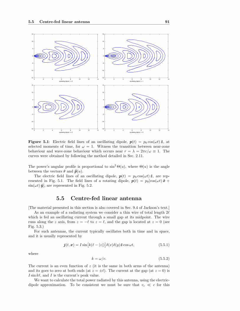
5.5 Centre-fed linear antenna 91
-15
-10
-5
0
5
10
15
0 2 4 6 8 10 12 14oscillating dipole: t = 0
-15
-10
-5
0
5
10
15
0 2 4 6 8 10 12 14oscillating dipole: t = 1
-15
-10
-5
0
5
10
15
0 2 4 6 8 10 12 14oscillating dipole: t = 2
-15
-10
-5
0
5
10
15
0 2 4 6 8 10 12 14oscillating dipole: t = 3
Figure 5.1: Electric field lines of an oscillating dipole, p(t) = p0 cos(ωt) z, atselected moments of time, for ω = 1. Witness the transition between near-zonebehaviour and wave-zone behaviour which occurs near r = λ = 2πc/ω ≡ 1. Thecurves were obtained by following the method detailed in Sec. 2.11.
The power’s angular profile is proportional to sin2 Θ(u), where Θ(u) is the anglebetween the vectors r and p(u).
The electric field lines of an oscillating dipole, p(t) = p0 cos(ωt) z, are rep-resented in Fig. 5.1. The field lines of a rotating dipole, p(t) = p0[cos(ωt) x +sin(ωt) y], are represented in Fig. 5.2.
5.5 Centre-fed linear antenna
[The material presented in this section is also covered in Sec. 9.4 of Jackson’s text.]As an example of a radiating system we consider a thin wire of total length 2ℓ
which is fed an oscillating current through a small gap at its midpoint. The wireruns along the z axis, from z = −ℓ to z = ℓ, and the gap is located at z = 0 (seeFig. 5.3.)
For such antennas, the current typically oscillates both in time and in space,and it is usually represented by
j(t,x) = I sin'
k(ℓ − |z|)(
δ(x)δ(y)z cos ωt, (5.5.1)
wherek = ω/c. (5.5.2)
The current is an even function of z (it is the same in both arms of the antenna)and its goes to zero at both ends (at z = ±ℓ). The current at the gap (at z = 0) isI sin kℓ, and I is the current’s peak value.
We want to calculate the total power radiated by this antenna, using the electric-dipole approximation. To be consistent we must be sure that vc ≪ c for this
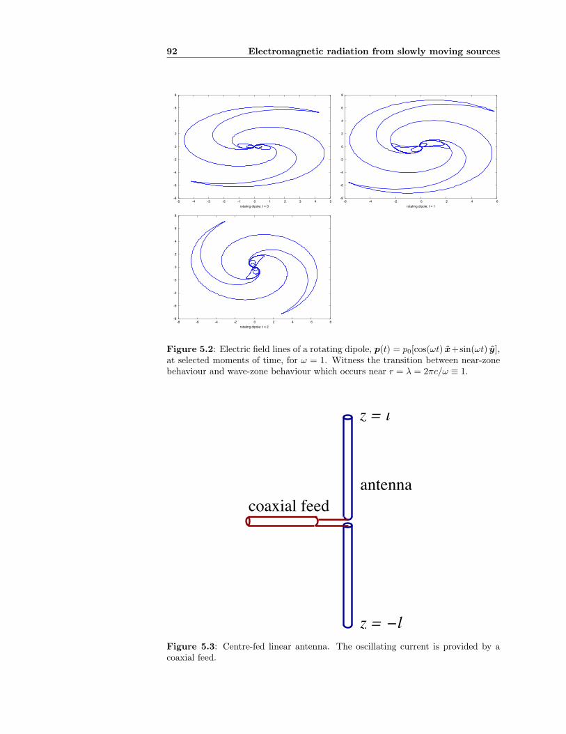
92 Electromagnetic radiation from slowly moving sources
-8
-6
-4
-2
0
2
4
6
8
-5 -4 -3 -2 -1 0 1 2 3 4 5rotating dipole: t = 0
-8
-6
-4
-2
0
2
4
6
8
-6 -4 -2 0 2 4 6rotating dipole: t = 1
-8
-6
-4
-2
0
2
4
6
8
-8 -6 -4 -2 0 2 4 6 8rotating dipole: t = 2
Figure 5.2: Electric field lines of a rotating dipole, p(t) = p0[cos(ωt) x+sin(ωt) y],at selected moments of time, for ω = 1. Witness the transition between near-zonebehaviour and wave-zone behaviour which occurs near r = λ = 2πc/ω ≡ 1.
coaxial feedantenna
z = l
z = −lFigure 5.3: Centre-fed linear antenna. The oscillating current is provided by acoaxial feed.
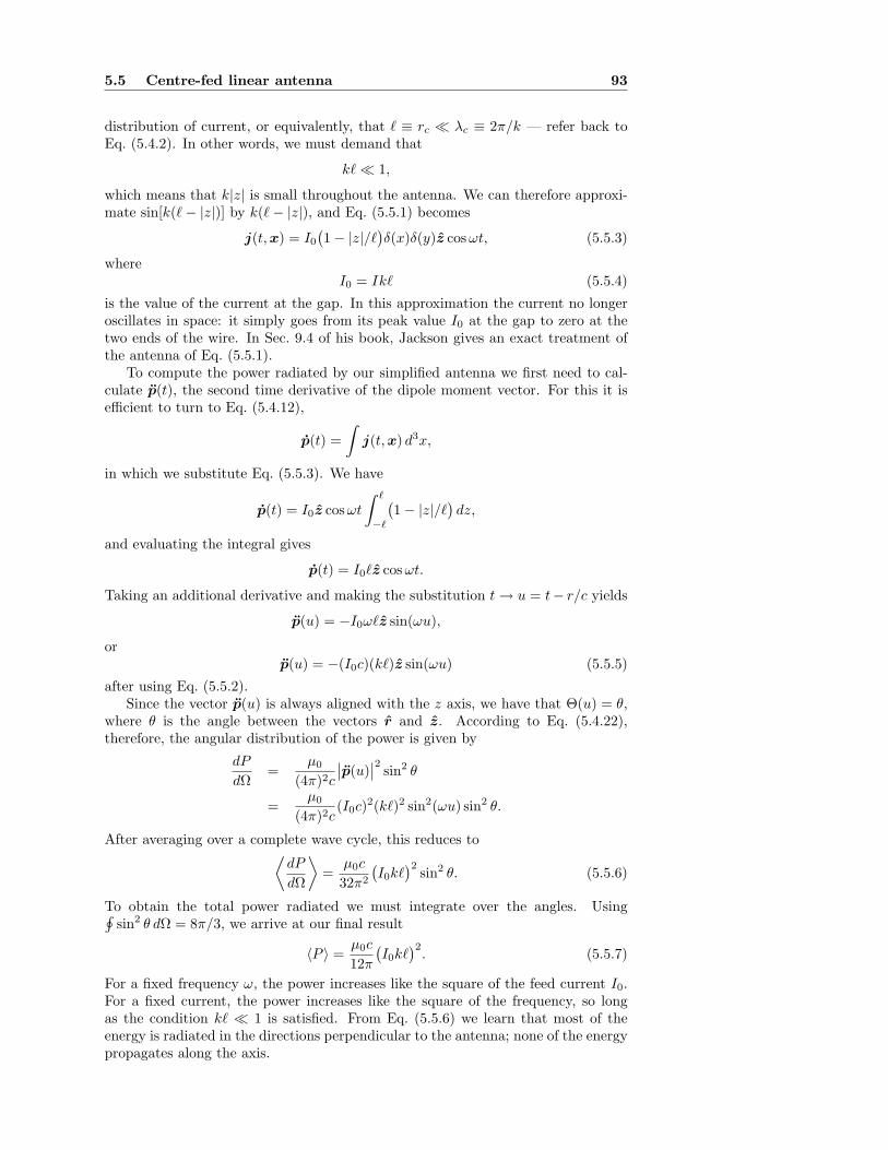
5.5 Centre-fed linear antenna 93
distribution of current, or equivalently, that ℓ ≡ rc ≪ λc ≡ 2π/k — refer back toEq. (5.4.2). In other words, we must demand that
kℓ ≪ 1,
which means that k|z| is small throughout the antenna. We can therefore approxi-mate sin[k(ℓ − |z|)] by k(ℓ − |z|), and Eq. (5.5.1) becomes
j(t,x) = I0
%
1 − |z|/ℓ&
δ(x)δ(y)z cos ωt, (5.5.3)
whereI0 = Ikℓ (5.5.4)
is the value of the current at the gap. In this approximation the current no longeroscillates in space: it simply goes from its peak value I0 at the gap to zero at thetwo ends of the wire. In Sec. 9.4 of his book, Jackson gives an exact treatment ofthe antenna of Eq. (5.5.1).
To compute the power radiated by our simplified antenna we first need to cal-culate p(t), the second time derivative of the dipole moment vector. For this it isefficient to turn to Eq. (5.4.12),
p(t) =
!
j(t,x) d3x,
in which we substitute Eq. (5.5.3). We have
p(t) = I0z cos ωt
! ℓ
−ℓ
%
1 − |z|/ℓ&
dz,
and evaluating the integral gives
p(t) = I0ℓz cos ωt.
Taking an additional derivative and making the substitution t → u = t− r/c yields
p(u) = −I0ωℓz sin(ωu),
orp(u) = −(I0c)(kℓ)z sin(ωu) (5.5.5)
after using Eq. (5.5.2).Since the vector p(u) is always aligned with the z axis, we have that Θ(u) = θ,
where θ is the angle between the vectors r and z. According to Eq. (5.4.22),therefore, the angular distribution of the power is given by
dP
dΩ=
µ0
(4π)2c
+
+p(u)+
+
2sin2 θ
=µ0
(4π)2c(I0c)
2(kℓ)2 sin2(ωu) sin2 θ.
After averaging over a complete wave cycle, this reduces to<
dP
dΩ
=
=µ0c
32π2
%
I0kℓ&2
sin2 θ. (5.5.6)
To obtain the total power radiated we must integrate over the angles. Using7
sin2 θ dΩ = 8π/3, we arrive at our final result
⟨P ⟩ =µ0c
12π
%
I0kℓ&2
. (5.5.7)
For a fixed frequency ω, the power increases like the square of the feed current I0.For a fixed current, the power increases like the square of the frequency, so longas the condition kℓ ≪ 1 is satisfied. From Eq. (5.5.6) we learn that most of theenergy is radiated in the directions perpendicular to the antenna; none of the energypropagates along the axis.
94 Electromagnetic radiation from slowly moving sources
5.6 Classical atom
The classical picture of a hydrogen atom contains a proton at the centre and anelectron on a circular orbit around it. Supposing for simplicity that the proton isat rest, the system’s dipole moment is p(t) = −ea(t) where a(t) is the electron’sposition vector. Since the electron is accelerated by the Lorentz force F exerted bythe proton, we have p(t) = −ea = −(e/m)F . Because this is nonzero, the atomemits electromagnetic radiation. The atom therefore loses energy to the radiation,and as a result, the orbital radius a gradually decreases; it eventually goes to zero.As is well known, the classical model leads to an unstable atom. In this section wecalculate the lifetime of the classical atom.
The Coulomb force exerted by the proton is
F = −1
4πϵ0
e2
a2a,
where a = a(t)/a. This gives
p(t) =1
4πϵ0
e
m
e2
a2a(t) (5.6.1)
for the second derivative of the dipole moment vector. According to the electric-dipole approximation, the total energy radiated by the atom per unit time is givenby Eq. (5.4.21),
P =µ0
6πc
+
+p(u)+
+
2.
Substituting Eq. (5.6.1) then gives
P =µ0
6πc
e6
(4πϵ0)2m2ca4. (5.6.2)
Energy conservation dictates that the energy carried away by the radiation mustcome at the expense of the atom’s orbital energy; we therefore have
dEorb
dt= −P. (5.6.3)
The orbital energy of a classical atom is
Eorb = −1
4πϵ0
e2
2a. (5.6.4)
Combining the last three equations, it is easy to show that the orbital radius mustdecrease, at a rate given by
da
dt= −
4
3
1
(4πϵ0)2e2
m2c3a2. (5.6.5)
To obtain the lifetime we integrate Eq. (5.6.5), starting with the initial conditionthat at t = 0, the orbital radius is equal to Bohr’s radius
a0 =4πϵ0!2
me2.
(In this step we make a leap and momentarily leave the classical realm, since theBohr radius is very much a consequence of quantum mechanics. But we maystill think of a0 as giving an appropriate initial condition, as it sets the atomic
5.7 Magnetic-dipole and electric-quadrupole radiation 95
length scale.) Integration of Eq. (5.6.5) is elementary, and we obtain τ ≡* τ0 dt =
* 0a0
(dt/da) da as
τ =(4πϵ0)5c3!6
4me10.
To put this in friendlier terms we introduce
α ≡e2
(4πϵ0)!c≃
1
137≡ fine structure constant (5.6.6)
and
λC ≡2π!
mc≃ 2.43 × 10⁻¹² m ≡ electron’s Compton wavelength. (5.6.7)
The lifetime can then be expressed as
τ =1
8πα5
λC
c≃ 1.6 × 10⁻¹¹ s. (5.6.8)
This result shows that under classical laws, the hydrogen atom would be extremelyshort lived. Equation (5.6.8), by the way, gives an order-of-magnitude estimate ofthe time required by an atom to make a transition from an excited state to theground state.
The results of this section, especially Eq. (5.6.5), leave us with a curious paradox.Ignoring the fact that the classical laws of electrodynamics do not apply to a realhydrogen atom, we seem to find an inconsistency in our description of the classicalatom. On the one hand, the fact that the electron feels the Coulomb field of theproton guarantees that the electron’s motion will be circular and that its orbitalradius will not change with time. (The most general orbit allowed by the Coulombforce is actually an ellipse, but the point remains that the size of this ellipse cannotchange with time.) On the other hand, we know that the electron is accelerated,that it emits electromagnetic waves, that the radiation carries energy away fromthe system, and that the orbital radius cannot possibly stay constant. The paradoxis therefore this: The electron’s equations of motion do not account for the decreasein orbital radius; they unambiguously predict that the radius should be constant.Is classical electrodynamics internally inconsistent?
Later on, in Chapter 6, we will show that the electron’s radiation reaction isactually contained in Maxwell’s theory. The effect is there, but it is well hidden,and it is a subtle matter to reveal it.
5.7 Magnetic-dipole and electric-quadrupole
radiation
[The material presented in this section is also covered in Sec. 9.3 of Jackson’s text.]Electric-dipole radiation corresponds to the leading-order approximation of the
electromagnetic field in an expansion in powers of vc/c, where vc is a typical internalvelocity of the source. In some cases, however, the dipole moment p either vanishesor does not depend on time, and the leading term is actually zero. In such cases, orwhen higher accuracy is required, we need to compute the next term in the expan-sion. This is our task in this section. We will see that at the next-to-leading-order,the wave-zone fields depend on the dipole moment vector p, the magnetic momentvector m, and the electric dipole moment tensor Qab. We recall the definitions ofthese objects:
p(t) =
!
Vρ(t,x′)x′ d3x′, (5.7.1)
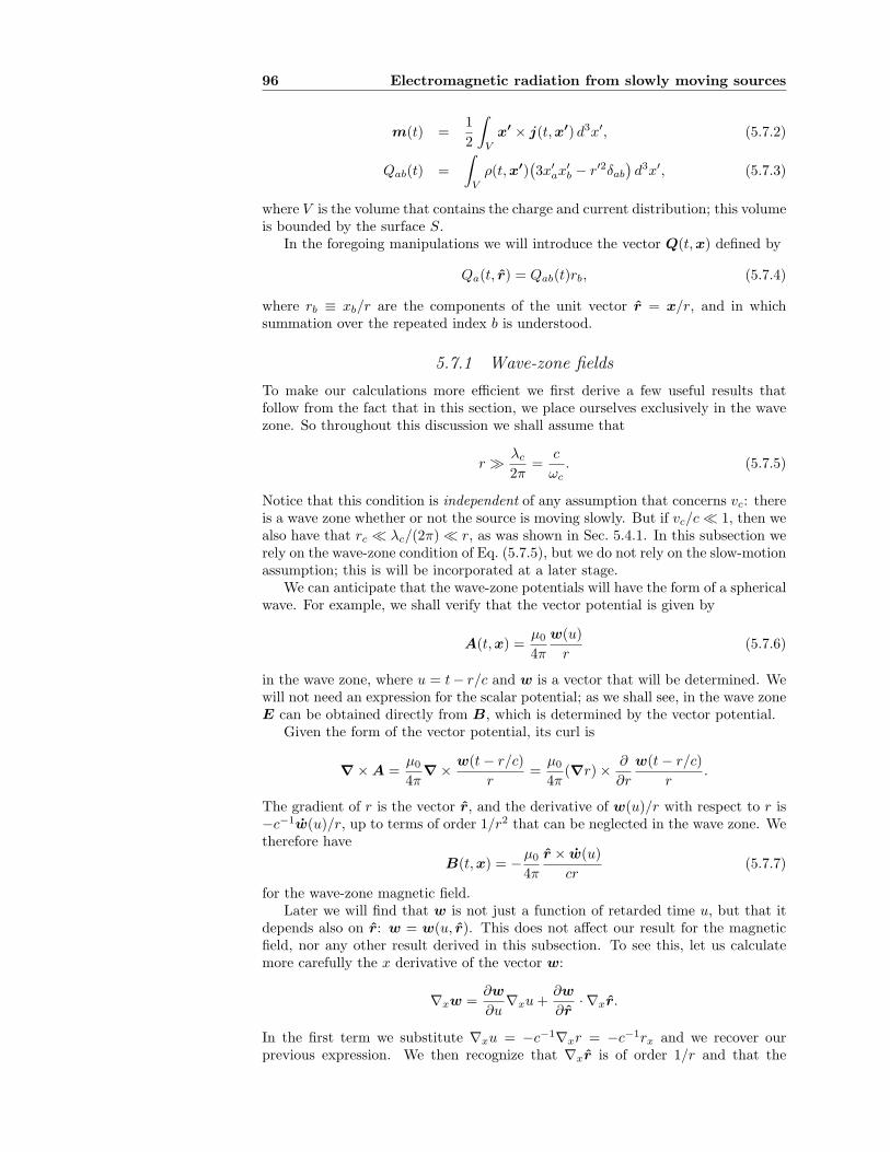
96 Electromagnetic radiation from slowly moving sources
m(t) =1
2
!
Vx′ × j(t,x′) d3x′, (5.7.2)
Qab(t) =
!
Vρ(t,x′)
%
3x′ax′
b − r′2δab
&
d3x′, (5.7.3)
where V is the volume that contains the charge and current distribution; this volumeis bounded by the surface S.
In the foregoing manipulations we will introduce the vector Q(t,x) defined by
Qa(t, r) = Qab(t)rb, (5.7.4)
where rb ≡ xb/r are the components of the unit vector r = x/r, and in whichsummation over the repeated index b is understood.
5.7.1 Wave-zone fields
To make our calculations more efficient we first derive a few useful results thatfollow from the fact that in this section, we place ourselves exclusively in the wavezone. So throughout this discussion we shall assume that
r ≫λc
2π=
c
ωc. (5.7.5)
Notice that this condition is independent of any assumption that concerns vc: thereis a wave zone whether or not the source is moving slowly. But if vc/c ≪ 1, then wealso have that rc ≪ λc/(2π) ≪ r, as was shown in Sec. 5.4.1. In this subsection werely on the wave-zone condition of Eq. (5.7.5), but we do not rely on the slow-motionassumption; this is will be incorporated at a later stage.
We can anticipate that the wave-zone potentials will have the form of a sphericalwave. For example, we shall verify that the vector potential is given by
A(t,x) =µ0
4π
w(u)
r(5.7.6)
in the wave zone, where u = t− r/c and w is a vector that will be determined. Wewill not need an expression for the scalar potential; as we shall see, in the wave zoneE can be obtained directly from B, which is determined by the vector potential.
Given the form of the vector potential, its curl is
∇ × A =µ0
4π∇ ×
w(t − r/c)
r=
µ0
4π(∇r) ×
∂
∂r
w(t − r/c)
r.
The gradient of r is the vector r, and the derivative of w(u)/r with respect to r is−c−1w(u)/r, up to terms of order 1/r2 that can be neglected in the wave zone. Wetherefore have
B(t,x) = −µ0
4π
r × w(u)
cr(5.7.7)
for the wave-zone magnetic field.Later we will find that w is not just a function of retarded time u, but that it
depends also on r: w = w(u, r). This does not affect our result for the magneticfield, nor any other result derived in this subsection. To see this, let us calculatemore carefully the x derivative of the vector w:
∇xw =∂w
∂u∇xu +
∂w
∂r·∇xr.
In the first term we substitute ∇xu = −c−1∇xr = −c−1rx and we recover ourprevious expression. We then recognize that ∇xr is of order 1/r and that the
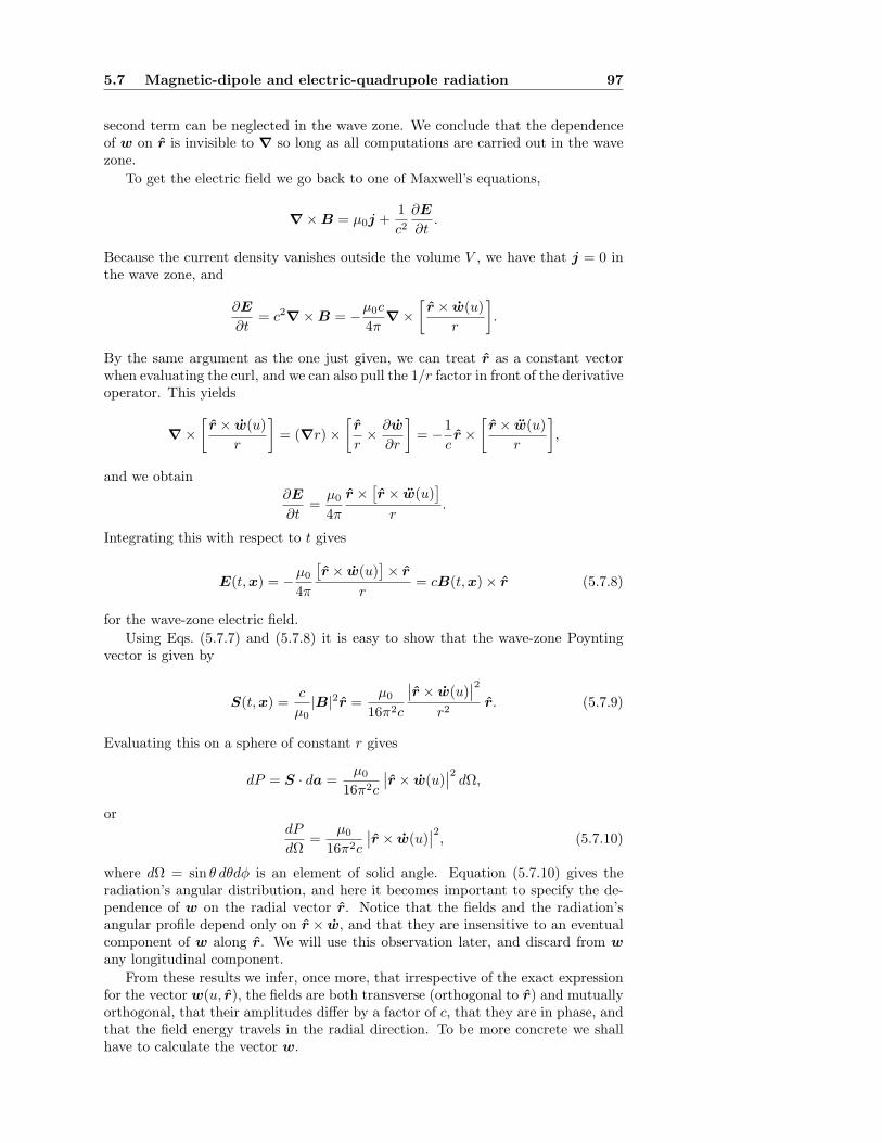
5.7 Magnetic-dipole and electric-quadrupole radiation 97
second term can be neglected in the wave zone. We conclude that the dependenceof w on r is invisible to ∇ so long as all computations are carried out in the wavezone.
To get the electric field we go back to one of Maxwell’s equations,
∇ × B = µ0j +1
c2
∂E
∂t.
Because the current density vanishes outside the volume V , we have that j = 0 inthe wave zone, and
∂E
∂t= c2
∇ × B = −µ0c
4π∇ ×
3
r × w(u)
r
4
.
By the same argument as the one just given, we can treat r as a constant vectorwhen evaluating the curl, and we can also pull the 1/r factor in front of the derivativeoperator. This yields
∇ ×3
r × w(u)
r
4
= (∇r) ×3
r
r×
∂w
∂r
4
= −1
cr ×
3
r × w(u)
r
4
,
and we obtain∂E
∂t=
µ0
4π
r ×'
r × w(u)(
r.
Integrating this with respect to t gives
E(t,x) = −µ0
4π
'
r × w(u)(
× r
r= cB(t,x) × r (5.7.8)
for the wave-zone electric field.Using Eqs. (5.7.7) and (5.7.8) it is easy to show that the wave-zone Poynting
vector is given by
S(t,x) =c
µ0|B|2r =
µ0
16π2c
+
+r × w(u)+
+
2
r2r. (5.7.9)
Evaluating this on a sphere of constant r gives
dP = S · da =µ0
16π2c
+
+r × w(u)+
+
2dΩ,
ordP
dΩ=
µ0
16π2c
+
+r × w(u)+
+
2, (5.7.10)
where dΩ = sin θ dθdφ is an element of solid angle. Equation (5.7.10) gives theradiation’s angular distribution, and here it becomes important to specify the de-pendence of w on the radial vector r. Notice that the fields and the radiation’sangular profile depend only on r × w, and that they are insensitive to an eventualcomponent of w along r. We will use this observation later, and discard from wany longitudinal component.
From these results we infer, once more, that irrespective of the exact expressionfor the vector w(u, r), the fields are both transverse (orthogonal to r) and mutuallyorthogonal, that their amplitudes differ by a factor of c, that they are in phase, andthat the field energy travels in the radial direction. To be more concrete we shallhave to calculate the vector w.
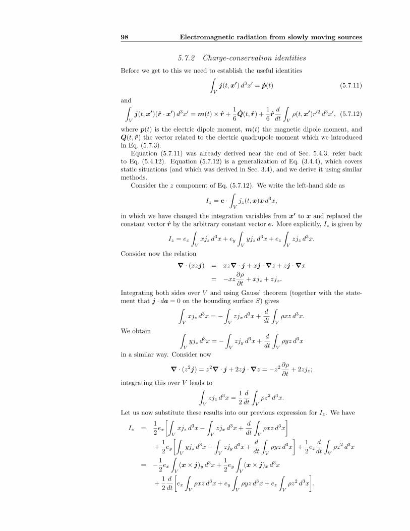
98 Electromagnetic radiation from slowly moving sources
5.7.2 Charge-conservation identities
Before we get to this we need to establish the useful identities!
Vj(t,x′) d3x′ = p(t) (5.7.11)
and!
Vj(t,x′)(r · x′) d3x′ = m(t) × r +
1
6Q(t, r) +
1
6r
d
dt
!
Vρ(t,x′)r′2 d3x′, (5.7.12)
where p(t) is the electric dipole moment, m(t) the magnetic dipole moment, andQ(t, r) the vector related to the electric quadrupole moment which we introducedin Eq. (5.7.3).
Equation (5.7.11) was already derived near the end of Sec. 5.4.3; refer backto Eq. (5.4.12). Equation (5.7.12) is a generalization of Eq. (3.4.4), which coversstatic situations (and which was derived in Sec. 3.4), and we derive it using similarmethods.
Consider the z component of Eq. (5.7.12). We write the left-hand side as
Iz = e ·!
Vjz(t,x)x d3x,
in which we have changed the integration variables from x′ to x and replaced theconstant vector r by the arbitrary constant vector e. More explicitly, Iz is given by
Iz = ex
!
Vxjz d3x + ey
!
Vyjz d3x + ez
!
Vzjz d3x.
Consider now the relation
∇ · (xzj) = xz∇ · j + xj · ∇z + zj · ∇x
= −xz∂ρ
∂t+ xjz + zjx.
Integrating both sides over V and using Gauss’ theorem (together with the state-ment that j · da = 0 on the bounding surface S) gives
!
Vxjz d3x = −
!
Vzjx d3x +
d
dt
!
Vρxz d3x.
We obtain!
Vyjz d3x = −
!
Vzjy d3x +
d
dt
!
Vρyz d3x
in a similar way. Consider now
∇ · (z2j) = z2∇ · j + 2zj · ∇z = −z2 ∂ρ
∂t+ 2zjz;
integrating this over V leads to!
Vzjz d3x =
1
2
d
dt
!
Vρz2 d3x.
Let us now substitute these results into our previous expression for Iz. We have
Iz =1
2ex
3!
Vxjz d3x −
!
Vzjx d3x +
d
dt
!
Vρxz d3x
4
+1
2ey
3!
Vyjz d3x −
!
Vzjy d3x +
d
dt
!
Vρyz d3x
4
+1
2ez
d
dt
!
Vρz2 d3x
= −1
2ex
!
V(x × j)y d3x +
1
2ey
!
V(x × j)x d3x
+1
2
d
dt
3
ex
!
Vρxz d3x + ey
!
Vρyz d3x + ez
!
Vρz2 d3x
4
.
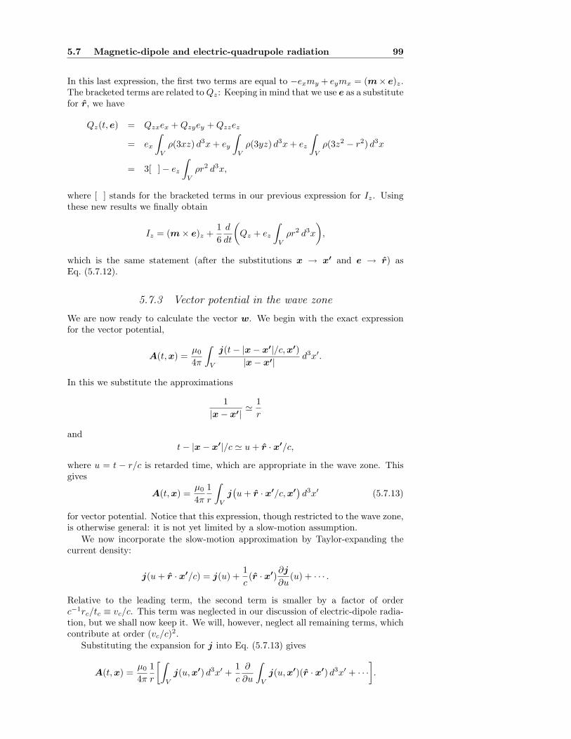
5.7 Magnetic-dipole and electric-quadrupole radiation 99
In this last expression, the first two terms are equal to −exmy + eymx = (m× e)z.The bracketed terms are related to Qz: Keeping in mind that we use e as a substitutefor r, we have
Qz(t,e) = Qzxex + Qzyey + Qzzez
= ex
!
Vρ(3xz) d3x + ey
!
Vρ(3yz) d3x + ez
!
Vρ(3z2 − r2) d3x
= 3[ ] − ez
!
Vρr2 d3x,
where [ ] stands for the bracketed terms in our previous expression for Iz. Usingthese new results we finally obtain
Iz = (m × e)z +1
6
d
dt
"
Qz + ez
!
Vρr2 d3x
#
,
which is the same statement (after the substitutions x → x′ and e → r) asEq. (5.7.12).
5.7.3 Vector potential in the wave zone
We are now ready to calculate the vector w. We begin with the exact expressionfor the vector potential,
A(t,x) =µ0
4π
!
V
j(t − |x − x′|/c,x′)
|x − x′|d3x′.
In this we substitute the approximations
1
|x − x′|≃
1
r
and
t − |x − x′|/c ≃ u + r · x′/c,
where u = t − r/c is retarded time, which are appropriate in the wave zone. Thisgives
A(t,x) =µ0
4π
1
r
!
Vj%
u + r · x′/c,x′&
d3x′ (5.7.13)
for vector potential. Notice that this expression, though restricted to the wave zone,is otherwise general: it is not yet limited by a slow-motion assumption.
We now incorporate the slow-motion approximation by Taylor-expanding thecurrent density:
j(u + r · x′/c) = j(u) +1
c(r · x′)
∂j
∂u(u) + · · · .
Relative to the leading term, the second term is smaller by a factor of orderc−1rc/tc ≡ vc/c. This term was neglected in our discussion of electric-dipole radia-tion, but we shall now keep it. We will, however, neglect all remaining terms, whichcontribute at order (vc/c)2.
Substituting the expansion for j into Eq. (5.7.13) gives
A(t,x) =µ0
4π
1
r
3!
Vj(u,x′) d3x′ +
1
c
∂
∂u
!
Vj(u,x′)(r · x′) d3x′ + · · ·
4
.
100 Electromagnetic radiation from slowly moving sources
According to Eq. (5.7.11), the first integral is equal to p(u). And according toEq. (5.7.12), the second integral is equal to
m(u) × r +1
6Q(u, r) +
1
6r
d
du
!
Vρ(u,x′)r′2 d3x′.
The quantity within the square brackets defines the vector w, and we have
w = p(u) +1
c
3
m(u) × r +1
6Q(u, r)
4
+1
6cr
d2
du2
!
Vρ(u,x′)r′2 d3x′.
The last term is proportional to r. But we have seen in Sec. 5.7.1 that the electricand magnetic fields, as well as the radiated power, depend only on r × w. Thismeans that any component of w along r will not contribute to the wave-zone fields.We can therefore discard this last term in our expression for w.
We have obtained
w(u, r) = p(u) +1
c
3
m(u) × r +1
6Q(u, r)
4
, (5.7.14)
and in terms of this the wave-zone vector potential is given by
A(t,x) =µ0
4π
w(u, r)
r, (5.7.15)
an expression that was already anticipated in Eq. (5.7.3). The first term on theright-hand side of Eq. (5.7.14) gives rise to electric-dipole radiation; this is theleading term in the expansion of the fields in powers of vc/c. The second andthird terms give rise to magnetic-dipole radiation and electric-quadrupole radiation,respectively; these contribute at order vc/c beyond the leading term.
To calculate the radiated power we shall need
r × w = r × p(u) +1
c
B
m(u) −'
r · m(u)(
rC
+1
6cr × Q(3)(u, r), (5.7.16)
where Q(3) ≡ ∂3Q/∂u3 and we have used the vectorial identity r × (m × r) =m − (r · m)r.
5.7.4 Radiated power (magnetic-dipole radiation)
Let us calculate the power radiated by a distribution of charges and currents forwhich
p(u) = Q(3)(u, r) = 0. (5.7.17)
Such a source will emit magnetic-dipole radiation.Under the conditions of Eq. (5.7.17), Eq. (5.7.16) becomes
r × w =1
c
1
m −%
r · m)r2
so that+
+r × w+
+
2=
1
c2
1
|m|2 − (r · m)22
,
which we rewrite in component form as
+
+r × w+
+
2=
1
c2mamb
%
δab − rarb
&
,
where ra = xa/r are the components of the vector r, and where summation overboth repeated indices is understood. Substituting this into Eq. (5.7.10) gives
dP
dΩ=
µ0
16π2c3mamb
%
δab − rarb
&
,
5.7 Magnetic-dipole and electric-quadrupole radiation 101
and integrating over the angles yields
P =µ0
4πc3mamb
%
δab − ⟨rarb⟩&
,
where
⟨rarb⟩ ≡1
4π
!
rarb dΩ =1
3δab.
These angular integrations are worked out in Sec. 5.7.7.Our final result for the radiated power is therefore
Pmagnetic-dipole =µ0
6πc3
+
+m(u)+
+
2. (5.7.18)
We might compare this result with Eq. (5.4.21),
Pelectric-dipole =µ0
6πc
+
+p(u)+
+
2.
In orders of magnitude we have that the electric dipole moment is p ∼ (ρrc)(r3c ) ∼
ρr4c and that p ∼ ρr4
c/t2c . On the other hand, m ∼ (jrc)(r3c ) ∼ jr4
c ∼ ρvcr4c , and
m ∼ ρvcr4c/t2c . The ratio of powers is then
Pmagnetic-dipole
Pelectric-dipole∼
"
m
cp
#2
∼"
vc
c
#2
.
So for slowing-moving sources, the power emitted in magnetic-dipole radiation istypically smaller than the power emitted in electric-dipole radiation by a factor oforder (vc/c)2 ≪ 1.
5.7.5 Radiated power (electric-quadrupole radiation)
Let us now calculate the power radiated by a distribution of charges and currentsfor which
p(u) = m(u) = 0. (5.7.19)
Such a source will emit electric-quadrupole radiation.Under the conditions of Eq. (5.7.19), Eq. (5.7.16) becomes
r × w =1
6cr × Q(3),
so that+
+r × w+
+
2=
1
36c2
%
r × Q(3)&
·%
r × Q(3)&
.
The inner product can be expressed as
(r · r)%
Q(3) · Q(3)&
−%
r · Q(3)&%
r · Q(3)&
=+
+Q(3)+
+
2 −%
r · Q(3)&2
,
and we have+
+r × w+
+
2=
1
36c2Q(3)
a Q(3)b
%
δab − rarb
&
.
But the vector Q(3) depends on r, because by the definition of Eq. (5.7.4), Qa =Qacrc. Writing also Qb = Qbdrd, we arrive at
+
+r × w+
+
2=
1
36c2Q(3)
ac Q(3)bd
%
δabrcrd − rarbrcrd
&
.
Substituting this into Eq. (5.7.10) gives
dP
dΩ=
µ0
16π2c
1
36c2Q(3)
ac Q(3)bd
%
δabrcrd − rarbrcrd
&
,
102 Electromagnetic radiation from slowly moving sources
and integrating over the angles yields
P =µ0
4πc
1
36c2Q(3)
ac Q(3)bd
%
δab⟨rcrd⟩ − ⟨rarbrcrd⟩&
.
The angular integrals
⟨rcrd⟩ ≡1
4π
!
rcrd dΩ =1
3δcd
and
⟨rarbrcrd⟩ ≡1
4π
!
rarbrcrd dΩ =1
15
,
δabδcd + δacδbd + δadδbc
-
are evaluated in Sec. 5.7.7. Taking these results into account, we obtain
Γ ≡ Q(3)ac Q(3)
bd
%
δab⟨rcrd⟩ − ⟨rarbrcrd⟩&
=1
3Q(3)
ac Q(3)bd δabδcd −
1
15Q(3)
ac Q(3)bd
%
δabδcd + δacδbd + δadδbc
&
=1
3Q(3)
ac Q(3)ac −
1
15Q(3)
ac Q(3)ac −
1
15Q(3)
aa Q(3)bb −
1
15Q(3)
ac Q(3)ca
=
"
1
3−
2
15
#
Q(3)ac Q(3)
ac
=1
5Q(3)
ac Q(3)ac ,
where we have used the property that Qab is a symmetric, tracefree tensor (so thatQca = Qac and Qaa = 0).
Our final result for the radiated power is therefore
Pelectric-quadrupole =µ0
720πc3Q(3)
ab (u)Q(3)ab (u), (5.7.20)
where summation over the two repeated indices is understood. In orders of mag-
nitude, Qab ∼ (ρr2c )(r3
c ) ∼ ρr5c , and Q(3)
ab ∼ ρr5c/t3c ∼ prc/tc ∼ pvc. We therefore
have
Pelectric-quadrupole
Pelectric-dipole∼
"
vc
c
#2
;
for slowing-moving distributions, the power emitted in electric-quadrupole radiationis smaller than the power emitted in electric-dipole radiation by a factor of order(vc/c)2 ≪ 1. We see also that electric-quadrupole radiation is of the same order ofmagnitude as magnetic-dipole radiation.
5.7.6 Total radiated power
In situations in which all three types of radiation contribute, the total power is thesum of individual contributions,
P =µ0
6πc
3
+
+p(u)+
+
2+
1
c2
+
+m(u)+
+
2+
1
120c2Q(3)
ab (u)Q(3)ab (u) + O
%
v4c/c4
&
4
. (5.7.21)
There is no interference between the different terms in Eq. (5.7.16), because theangular profiles associated with each term are orthogonal.
5.8 Pulsar spin-down 103
5.7.7 Angular integrations
In this subsection we establish the formulae
⟨ra⟩ = 0, (5.7.22)
⟨rarb⟩ =1
3δab, (5.7.23)
⟨rarbrc⟩ = 0, (5.7.24)
⟨rarbrcrd⟩ =1
15
,
δabδcd + δacδbd + δadδbc
-
, (5.7.25)
where ra = xa/r are the components of the vector r, and ⟨· · ·⟩ ≡ (4π)−1*
(· · ·) dΩis the average of the quantity (· · ·) over a sphere of constant r.
These relations can be derived by brute-force computation, by simply substi-tuting r = (sin θ cos φ, sin θ sinφ, cos θ) and integrating over dΩ = sin θ dθdφ. Butthere is an easier, prettier way that relies on arguments of symmetry.
Take the zero result for ⟨ra⟩. If these integrals were not zero, they would have tobe equal to some vector a that does not depend on the angles θ and φ (because theyhave been integrated over) nor on r (because r appears nowhere on the left-handside of the equation). But there is no such vector available, because there is nopreferred direction in a homogeneous three-dimensional space. The right-hand sidemust therefore be zero.
To arrive at the result for ⟨rarb⟩ we observe that the right-hand side must bea constant tensor that is symmetric in the pair of indices a and b. The only suchtensor available is δab, and we must therefore have ⟨rarb⟩ = λδab, for some constantλ. To determine λ we simply take the trace of the left-hand side,
δab⟨rarb⟩ = ⟨δabrarb⟩ = ⟨1⟩ = 1,
and the trace of the right-hand side,
λδabδab = 3λ.
Equating the results produces λ = 1/3, and this agrees with the result of Eq. (5.7.23).The zero result for ⟨rarbrc⟩ follows from the fact that we do not have a vector
that could be combined with δab to form a symmetric, three-index tensor.To derive the result for ⟨rarbrcrd⟩ we note that the right-hand side must be a
four-index tensor that is symmetric in all pairs of indices. We must form this tensorwith two copies of δab, and it is easy to see that it must be equal to λ′(δabδcd +δacδbd + δadδbc). To determine λ′ we evaluate the double trace of the left-hand side,which gives 1, and the double trace of the right-hand side, which gives
λ′δabδcd
%
δabδcd + δacδbd + δadδbc
&
= λ′(3 × 3 + 3 + 3) = 15λ′.
Equating the results produces λ′ = 1/15, in agreement with Eq. (5.7.24).
5.8 Pulsar spin-down
As an application of magnetic-dipole radiation we consider the oblique-rotator modelof a pulsar, a rotating neutron star that emits pulses of electromagnetic radiationat regular intervals. The most famous pulsar is located in the Crab nebula, and thepulsar is believed to be the source of energy for this supernova remnant.
The Crab pulsar is observed to spin down: the frequency of the pulses decreaseswith time. If we associate the pulse frequency with the neutron star’s spin frequency,
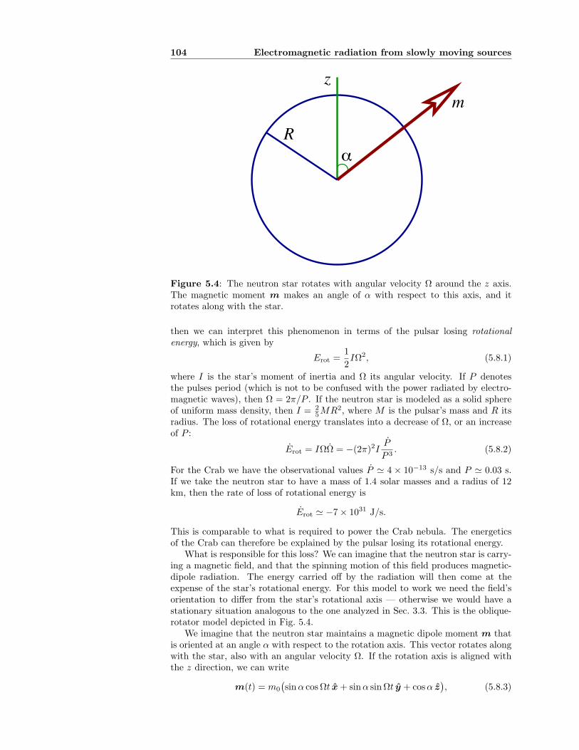
104 Electromagnetic radiation from slowly moving sources
αR
zm
Figure 5.4: The neutron star rotates with angular velocity Ω around the z axis.The magnetic moment m makes an angle of α with respect to this axis, and itrotates along with the star.
then we can interpret this phenomenon in terms of the pulsar losing rotationalenergy, which is given by
Erot =1
2IΩ2, (5.8.1)
where I is the star’s moment of inertia and Ω its angular velocity. If P denotesthe pulses period (which is not to be confused with the power radiated by electro-magnetic waves), then Ω = 2π/P . If the neutron star is modeled as a solid sphereof uniform mass density, then I = 2
5MR2, where M is the pulsar’s mass and R itsradius. The loss of rotational energy translates into a decrease of Ω, or an increaseof P :
Erot = IΩΩ = −(2π)2IP
P 3. (5.8.2)
For the Crab we have the observational values P ≃ 4 × 10⁻¹³ s/s and P ≃ 0.03 s.If we take the neutron star to have a mass of 1.4 solar masses and a radius of 12km, then the rate of loss of rotational energy is
Erot ≃ −7 × 1031 J/s.
This is comparable to what is required to power the Crab nebula. The energeticsof the Crab can therefore be explained by the pulsar losing its rotational energy.
What is responsible for this loss? We can imagine that the neutron star is carry-ing a magnetic field, and that the spinning motion of this field produces magnetic-dipole radiation. The energy carried off by the radiation will then come at theexpense of the star’s rotational energy. For this model to work we need the field’sorientation to differ from the star’s rotational axis — otherwise we would have astationary situation analogous to the one analyzed in Sec. 3.3. This is the oblique-rotator model depicted in Fig. 5.4.
We imagine that the neutron star maintains a magnetic dipole moment m thatis oriented at an angle α with respect to the rotation axis. This vector rotates alongwith the star, also with an angular velocity Ω. If the rotation axis is aligned withthe z direction, we can write
m(t) = m0
%
sin α cos Ωt x + sin α sin Ωt y + cos α z&
, (5.8.3)
5.9 Problems 105
where m0 is the magnitude of the pulsar’s magnetic moment. This can be relatedto the magnitude of the magnetic field on the surface of the neutron star. Becausethe star is located well within the near zone, we can use Eq. (3.4.2) to describe thesurface field:
B =µ0
4π
3(m · r)r − m
R3,
where R is the star’s radius. The field is maximum at the magnetic pole, where ris aligned with m. We therefore have
Bmax =µ0
4π
2m0
R3, (5.8.4)
a relationship between m0, the star’s radius, and the maximum surface magneticfield.
The time-changing magnetic moment of Eq. (5.8.3) produces magnetic-dipoleradiation. This radiation takes energy away from the star, at a rate given byEq. (5.7.18),
Erad =µ0
6πc3
+
+m(u)+
+
2,
where u = t − r/c is retarded time. Substituting Eq. (5.8.3) gives
Erad =µ0
6πc3
%
m0Ω2 sinα
&2, (5.8.5)
or
Erad =2π
3µ0c3
%
BmaxΩ2R3 sinα
&2(5.8.6)
after involving Eq. (5.8.4).To produce an equality between Erad and |Erot| ≃ 7 × 1031 J/s, we need a
magnetic field such thatBmax sinα ≃ 5 × 10⁸ T.
This is very large, but not unreasonable. A main-sequence star typically supports amagnetic field of 0.1 T. When the star collapses to form a neutron star, the magneticfield is frozen in and the magnetic flux 4πR2B is conserved. Because R decreasesby a factor of 105 during the collapse, B increases by a factor of 1010, and fields ofthe order of 108 T can easily be achieved for neutron stars.
5.9 Problems
1. A point electric dipole is rotating around the z axis at an angular velocity ω,so that
p(t) = p0
'
cos(ωt) x + sin(ωt) y(
,
where p0 is a constant.
a) Calculate the wave-zone electric and magnetic fields of this rotating dipole.Express the fields in terms of the unit vectors θ and φ.
b) Calculate ⟨dP/dΩ⟩, the angular profile of the radiated power, averagedover a complete wave cycle.
c) Calculate the total radiated power. How does it compare with the powerradiated by an oscillating dipole?
2. Two equal charges q are moving with constant angular velocity Ω on a circleof radius b. The charges are situated at diametrically opposite points on thecircle. Calculate, to leading order in a slow-motion approximation, the totalpower radiated by this distribution of charges.
106 Electromagnetic radiation from slowly moving sources
3. The current density inside a centre-fed, linear antenna is given by
j(t,x) = I cos(ωt) sin(kℓ − k|z|)δ(x)δ(y) z,
where I is the current’s peak amplitude, ω the oscillation frequency, ℓ theantenna’s half-length, and k = ω/c. In this problem we do not impose theslow-motion approximation, so that kℓ is not assumed to be small.
a) Show that in the wave zone (kr ≫ 1), the vector potential can be expressedas
A(t,x) =µ0
4π
w(u, θ)
r,
and find an expression for the vector w(u, θ). Here, u = t−r/c is retardedtime and θ is the angle between x and the z axis.
b) Calculate ⟨dP/dΩ⟩, the angular profile of the radiated power, averagedover a complete wave cycle. For the two special cases kℓ = π/2 (half-wave antenna) and kℓ = π (full-wave antenna), provide parametric plotsof this angular profile (like those displayed in Jackson’s Figure 9.7). Com-pare these profiles with the sin2 θ dependence obtained for electric-dipoleradiation.
c) From the general expression for ⟨dP/dΩ⟩ derived in part b), obtain theshort-antenna limit kℓ ≪ 1. Make sure that your result matches the onederived in the text.
4. An oscillating current I(t) = I0e−γt sin(ωt) flows in a circular loop of radius aplaced in the equatorial plane of the coordinate system (r, θ,φ). The currentis started at t = 0, and it decays exponentially due to dissipation within theloop; we assume that γ ≪ ω, so that the time scale for dissipation is muchlonger than the oscillation period. The current density is given by
j(t,x) =I(t)
aδ(r − a)δ(θ − π/2) φ.
Calculate ⟨P ⟩, the total power radiated by the loop, averaged over an os-cillation period. Calculate also the total amount of energy radiated by theloop.
5. A nearly spherical surface described by
r = R(t, θ) ≡ a(1 + ϵ cos θ cos ωt),
where a, ω, and ϵ are constants, supports a nearly uniform distribution ofcharge. It is assumed that ϵ ≪ 1, and the charge density is given by
ρ(t,x) =q
4πa2δ%
r − R(t, θ)&
,
where q is the total charge.
Calculate ⟨P ⟩, the electromagnetic power emitted by this distribution ofcharge, averaged over a complete wave cycle. You may work to leading orderin the slow-motion approximation. You may also work to leading order in ϵ.
6. A ring of radius b is placed in the x-y plane, and the origin of the coordinatesystem is placed at the centre of the ring. Initially, the ring is at rest and itsupports a linear charge density proportional to sinφ, where φ is the anglefrom the x-axis. The ring is then made to rotate with a uniform angularvelocity Ω, so that the linear charge density becomes proportional to sin(φ −Ωt). The ring’s volume charge density is described by
ρ(t, r, θ,φ) =λ
bδ(r − b)δ(θ − π
2 ) sin(φ − Ωt).
5.9 Problems 107
(a) Calculate, to leading order in a slow-motion approximation, the totalpower radiated by the ring. At what angle θ is most of the radiationemitted?
(b) Find an exact expression for Φ(t,0), the scalar potential at the centre ofthe ring.
(c) Find an exact expression for A(t,0), the vector potential at the centre ofthe ring.
7. Three charges are located along the z axis: a charge +2q stays at the originz = 0, a charge −q is at z = +a cos ωt, and the final charge −q is at z =−a cos ωt; a and ω are constants. It is assumed that aω ≪ 2πc and that thecharges simply go through one another when they meet at z = 0.
For this situation calculate ⟨dP/dΩ⟩, the angular profile of the radiated power,averaged over a complete wave cycle. (Express this in terms of the angle θfrom the z axis.) Calculate also ⟨P ⟩, the total radiated power. What is thefrequency of the electromagnetic waves emitted by this system of charges?
8. A current I is suddenly established in an infinite wire that extends along thez axis. The current density is given by
j(t,x) = Iθ(t)δ(x)δ(y)z,
where θ(t) is the step function. Because ∇ · j = 0, it is consistent to setρ(t,x) = 0.
Calculate, without approximations, the vector potential A(t,x) associatedwith this distribution of current. From your answer you should be able toverify that at late times, the electric and magnetic fields that are producedby the distribution of current have the components
Ez ≃ −µ0
4π
2I
t, Bx ≃ −
µ0
4π
2Iy
x2 + y2, By ≃
µ0
4π
2Ix
x2 + y2.
The electric field eventually disappears, and the magnetic field settles downto the value it would have for an unchanging current.

108 Electromagnetic radiation from slowly moving sources
Chapter 6
Electrodynamics of point
charges
6.1 Lorentz transformations
[The material presented in this section is also covered in Secs. 11.3, 11.9, and 11.10of Jackson’s text.]
In this final chapter we will look at the electrodynamics of charge and currentdistributions for which the characteristic speed vc is close to the speed of light. Tokeep the discussion concrete we will restrict it to the electromagnetic field producedby a single point particle in arbitrary (relativistic) motion. To set the stage webegin with a review of the Lorentz transformations of special relativity.
We consider a reference frame S′ that moves with constant speed v relative toanother frame S; we take the motion to take place in the x direction, so that theframe’s velocity vector is v = vx. The coordinates (t′, x′, y′, z′) of an event seenin S′ are related to the coordinates (t, x, y, z) of the same event seen in S by thewell-known relations
x′ = γ(x − vt), y′ = y, z′ = z, t′ = γ
"
t −v
c2x
#
, (6.1.1)
where
γ =1
0
1 − v2/c2. (6.1.2)
These are the Lorentz transformations between the two reference frames. The re-versed transformation is obtained by reversing the sign of v:
x = γ(x′ + vt′), y = y′, z = z′, t = γ
"
t′ +v
c2x′
#
. (6.1.3)
We now would like to derive how the electric and magnetic fields transform undersuch a change of reference frame.
We note first that Lorentz transformations alter the differential operators. Forexample, applying the chain rule on an arbitrary function ψ gives
∂ψ
∂t′=
∂ψ
∂t
∂t
∂t′+
∂ψ
∂x
∂x
∂t′+
∂ψ
∂y
∂y
∂t′+
∂ψ
∂z
∂z
∂t′,
or∂ψ
∂t′= γ
"
∂ψ
∂t+ v
∂ψ
∂x
#
109
110 Electrodynamics of point charges
after using Eq. (6.1.3). Doing a similar calculation for all other partial derivatives,we obtain
∂
∂x′= γ
"
∂
∂x+
v
c2
∂
∂t
#
,∂
∂y′=
∂
∂y,
∂
∂z′=
∂
∂z,
∂
∂t′= γ
"
∂
∂t+ v
∂
∂x
#
.
(6.1.4)It follows from this that the wave operator is a Lorentz invariant:
!′ψ = −
1
c2
∂2ψ
∂t′2+
∂2ψ
∂x′2+
∂2ψ
∂y′2+
∂2ψ
∂z′2
= −1
c2γ2
"
∂
∂t+ v
∂
∂x
#"
∂
∂t+ v
∂
∂x
#
ψ
+ γ2
"
∂
∂x+
v
c2
∂
∂t
#"
∂
∂x+
v
c2
∂
∂t
#
ψ +∂2ψ
∂y2+
∂2ψ
∂z2
= −1
c2
∂2ψ
∂t2+
∂2ψ
∂x2+
∂2ψ
∂y2+
∂2ψ
∂z2
= !ψ.
In other words,!
′ = !. (6.1.5)
To figure out how the electric and magnetic fields transform under a change ofreference frame, we first work out how ρ and j should transform. This will tell ushow the potentials Φ and A transform, and from this we will be able to get to thefields.
It is sufficient to consider a simple special case: a point charge q moving in thex direction with a speed v (the same speed that enters in the Lorentz transforma-tion). As seen from S we have ρ = qδ(x − vt)δ(y)δ(z), jx = qvδ(x − vt)δ(y)δ(z),and jy = jz = 0. As seen from S′, however, the particle is not moving, andρ′ = qδ(x′)δ(y′)δ(z′), while j′x = j′y = j′z = 0. We can expect that the Lorentztransformation will involve a linear mixture of ρ and jx, and that the other compo-nents of the current density will be left alone. Rewriting ρ′ in terms of the unprimedcoordinates gives
ρ′ = qδ[γ(x + vt)]δ(y)δ(z)
=q
γδ(x − vt)δ(y)δ(z).
This expression for ρ′ involves a factor of 1/γ instead of the expected γ, and jx hasnot yet made an appearance. But we can write it in the equivalent form
ρ′ = qγ(1 − v2/c2)δ(x − vt)δ(y)δ(z)
= γ
3
qδ(x − vt)δ(y)δ(z) −v
c2qvδ(x − vt)δ(y)δ(z)
4
= γ
"
ρ −v
c2jx
#
,
and this is the expected expression of a Lorentz transformation. This shows thatρ transforms as t, and we further expect that jx will transform as x, that is, j′x =γ(jx − vρ). This is confirmed by the fact that the right-hand side is zero for thesituation considered here. We conclude that under a change of reference frame, thecharge and current densities transform as
j′x = γ(jx − vρ), j′y = jy, j′z = jz, ρ′ = γ
"
ρ −v
c2jx
#
. (6.1.6)
6.1 Lorentz transformations 111
While the derivation of these transformation rules was restricted to a very simplesituation, it is possible to show that they are in fact completely general.
To see how the potentials transform we recall the wave equations !(Φ/c2) =−ρ/(ϵ0c2) = −µ0ρ and !A = −µ0j from Sec. 5.1. Because ! is an invariant, theseequations tell us that Φ/c2 must transform as ρ, and that A must transform as j.Thus,
A′x = γ
"
Ax −v
c2Φ
#
, A′y = Ay, A′
z = Ax, Φ′ = γ(Φ − vAx) (6.1.7)
are the Lorentz transformations for the scalar and vector potentials. These aredesigned to leave the form of the wave equations unchanged under a change ofreference frame. You should check that the Lorenz gauge condition,
∇ · A +1
c2
∂Φ
∂t= 0,
also takes the same form in S′. All the equations satisfied by the potentials aretherefore preserved under a Lorentz transformation. This implies that Maxwell’sequations themselves are invariant under a change of reference frame.
We can now figure out how the fields transform. We simply write down how thefields in S′ are related to the potentials,
E′ = −∂A′
∂t′− ∇
′Φ′, B′ = ∇′ × A′,
and we substitute Eqs. (6.1.4) and (6.1.7). For example,
E′x = −γ2
"
∂
∂t+ v
∂
∂x
#"
Ax −v
c2Φ
#
− γ2
"
∂
∂x+
v
c2
∂
∂t
#
,
Φ − vAx
-
= −∂Ax
∂t−
∂Φ
∂x= Ex.
Or
E′y = −γ
"
∂
∂t+ v
∂
∂x
#
Ay − γ∂
∂y
,
Φ − vAx
-
= −γ
"
∂Ay
∂t+
∂Φ
∂y
#
− γv
"
∂Ay
∂x−
∂Ax
∂y
#
= γ%
Ey − vBz
&
.
Another example is
B′x =
∂A′z
∂y′−
∂A′y
∂z′=
∂Az
∂y−
∂Ay
∂z= Bx.
Yet another is
B′y =
∂A′x
∂z′−
∂A′z
∂x′
= γ∂
∂z
"
Ax −v
c2Φ
#
− γ
"
∂
∂x+
v
c2
∂
∂t
#
Az
= γ
"
∂Ax
∂z−
∂Az
∂x
#
+ γv
c2
"
−∂Az
∂t−
∂Φ
∂z
#
= γ
"
By +v
c2Ez
#
.
112 Electrodynamics of point charges
The complete summary of these results is that the electric field transforms as
E′x = Ex, E′
y = γ%
Ey − vBz
&
, E′z = γ
%
Ez + vBy
&
(6.1.8)
under a change of reference frame, while the magnetic field transforms as
B′x = Bx, B′
y = γ
"
By +v
c2Ez
#
, B′z = γ
"
Bz −v
c2Ey
#
. (6.1.9)
Two observers in relative motion will therefore disagree as to the value of the electricand magnetic fields.
There are interesting special cases to the foregoing results. Suppose first thatB = 0 in some reference frame S. In another reference frame S′ we have E′
x = Ex,E′
y = γEy, E′z = γEz, B′
x = 0, B′y = γ(v/c2)Ez = (v/c2)E′
z = −(v × E′)y/c2, andB′
z = −γ(v/c2)Ey = −(v/c2)E′y = −(v × E′)z/c2. In other words,
B = 0 → B′ = −1
c2v × E′. (6.1.10)
A pure electric field in S is therefore perceived as a mixture of electric and magneticfields in S′. Suppose next that E = 0 in S. Then B′
x = Bx, B′y = γBy, B′
z = γBz,E′
x = 0, E′y = −γvBz = −vB′
z = (v × B′)y, and E′z = γvBy = vB′
y = (v × B′)z.In other words,
E = 0 → E′ = v × B′. (6.1.11)
A pure magnetic field in S is therefore perceived as a mixture of electric and mag-netic fields in S′. We conclude that E and B are observer-dependent fields; onlythe electromagnetic field as a whole has an observer-independent existence.
6.2 Fields of a uniformly moving charge
[The material presented in this section is also covered in Sec. 11.10 of Jackson’stext.]
We can use the Lorentz transformations of Eqs. (6.1.8) and (6.1.9) to calculatethe electric and magnetic fields of a point charge q that moves with constant speedv in the x direction. The charge’s position vector is
r(t) = (vt, b, 0), (6.2.1)
where b is the charge’s displacement above the x axis. We want E and B asmeasured at O, the origin of the reference frame S. We shall first do the calculationin S′, which moves along with the particle.
As seen in the reference frame S′, the charge’s position vector is r′ = (0, b, 0),but the observer at O has a position r′
O = (−vt′, 0, 0), because relative to S′, Omoves in the negative x direction with speed v. In S′ there is only an electric fieldE′, and its value at O is given by the standard expression
E′ = −q
4πϵ0
r′ − r′
O
|r′ − r′
O|3.
We have r′ − r′
O = (vt′, b, 0), |r′ − r′
O| =√
b2 + v2t′2, and the primed componentsof the electric field are
E′x = −
q
4πϵ0
vt′
(b2 + v2t′2)3/2, E′
y = −q
4πϵ0
b
(b2 + v2t′2)3/2, E′
z = 0. (6.2.2)
As measured in S′, the electric field lines are distributed isotropically around r′,the charge’s position.
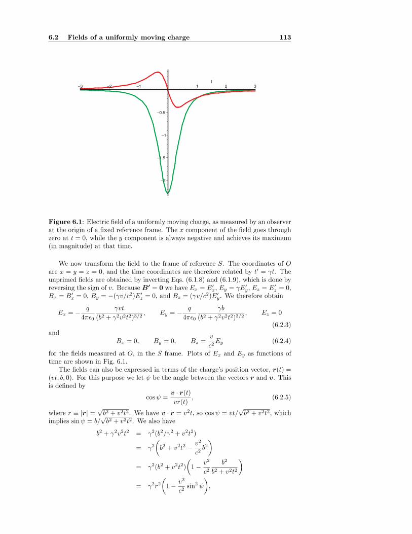
6.2 Fields of a uniformly moving charge 113
–2
–1.5
–1
–0.5
–3 –2 –1 1 2 3t
Figure 6.1: Electric field of a uniformly moving charge, as measured by an observerat the origin of a fixed reference frame. The x component of the field goes throughzero at t = 0, while the y component is always negative and achieves its maximum(in magnitude) at that time.
We now transform the field to the frame of reference S. The coordinates of Oare x = y = z = 0, and the time coordinates are therefore related by t′ = γt. Theunprimed fields are obtained by inverting Eqs. (6.1.8) and (6.1.9), which is done byreversing the sign of v. Because B′ = 0 we have Ex = E′
x, Ey = γE′y, Ez = E′
z = 0,Bx = B′
x = 0, By = −(γv/c2)E′z = 0, and Bz = (γv/c2)E′
y. We therefore obtain
Ex = −q
4πϵ0
γvt
(b2 + γ2v2t2)3/2, Ey = −
q
4πϵ0
γb
(b2 + γ2v2t2)3/2, Ez = 0
(6.2.3)and
Bx = 0, By = 0, Bz =v
c2Ey (6.2.4)
for the fields measured at O, in the S frame. Plots of Ex and Ey as functions oftime are shown in Fig. 6.1.
The fields can also be expressed in terms of the charge’s position vector, r(t) =(vt, b, 0). For this purpose we let ψ be the angle between the vectors r and v. Thisis defined by
cos ψ =v · r(t)
vr(t), (6.2.5)
where r ≡ |r| =√
b2 + v2t2. We have v · r = v2t, so cos ψ = vt/√
b2 + v2t2, whichimplies sinψ = b/
√b2 + v2t2. We also have
b2 + γ2v2t2 = γ2(b2/γ2 + v2t2)
= γ2
"
b2 + v2t2 −v2
c2b2
#
= γ2(b2 + v2t2)
"
1 −v2
c2
b2
b2 + v2t2
#
= γ2r2
"
1 −v2
c2sin2 ψ
#
,
114 Electrodynamics of point charges
and this can be substituted into Eqs. (6.2.3). The end result is
E = −q
4πϵ0
1
γ2'
1 − (v/c)2 sin2 ψ(3/2
r
r3(6.2.6)
for the electric field at O, and
B =1
c2v × E (6.2.7)
for the magnetic field.We see from Eq. (6.2.6) that E is always directed along −r(t), a vector that
points from the charge to O. The electric field therefore points away from the charge,and this means that the electric field lines originate at the position of the movingcharge. The field lines, however, are not distributed isotropically around the charge;this is revealed by the presence of sin2 ψ in the expression for the electric field. Whenψ = 0, that is, when r is directed along v, we have that [1− (v/c)2 sin2 ψ]−3/2 = 1,and the electric field is reduced by a relativistic factor of γ−2 < 1. But when insteadψ = π/2, so that r is orthogonal to v, then [1−(v/c)2 sin2 ψ]−3/2 = γ3 > 1, and thefield is amplified by a factor γ > 1. The electric field, as seen in S, is strongest inthe directions transverse to the motion, and weakest in the longitudinal direction.
The results derived in this section are at once remarkable and unremarkable. Itis unremarkable that the field lines should emanate from the position of the charge— we have the same picture in the charge’s rest frame. And it is unremarkable thatthe field lines should be distorted by a Lorentz contraction in the direction of themotion. But it is remarkable that the field registered at O does not involve a timedelay associated with the propagation of a signal from charge to observer.
Allowing for such a delay would suggest that the field at time t should point nottoward the charge at its current position r(t), but instead toward an earlier positionr(t′). In this picture, a signal originates at the charge when it was at the earlierposition, and it propagates to O in a time ∆t ≡ t − t′ determined by the conditionthat the signal travels at the speed of light; since the distance traveled is |r(t′)|,we must have t − t′ = |r(t′)|/c, which in principle can be solved for t′. Duringthe time in which the signal propagates, the particle moves to its current position,but the field registered at O should not yet be aware of this; it should know onlyof the earlier position, and E should therefore point in the direction of r(t′). Butthis is not what we have found: the field does point in the direction of r(t), thecurrent position of the charge. Our picture, according to which information shouldbe delayed, is curiously wrong. We will return to this issue later on, and investigateit more fully.
6.3 Fields of an arbitrarily moving charge
[The material presented in this section is also covered in Secs. 6.5 and 14.1 ofJackson’s text.]
We now allow the point charge q to move on an arbitrary trajectory r(t). Welet v(t) = dr/dt be its velocity vector, and a(t) = dv/dt its acceleration vector.The charge density is
ρ(t,x) = qδ%
x − r(t)&
, (6.3.1)
and the current density is
j(t,x) = qv(t)δ%
x − r(t)&
. (6.3.2)
To obtain the fields produced by this particle we shall first calculate the potentials.
6.3 Fields of an arbitrarily moving charge 115
6.3.1 Potentials
To calculate the potentials associated with the densities of Eqs. (6.3.1) and (6.3.2)we employ a technique that was first put to use in Secs. 5.2 and 5.3. For example,we express the vector potential as
A(t,x) =µ0
4π
!
j(t′,x′)δ(t − t′ − |x − x′|/c)
|x − x′|d3x′dt′,
in terms of the retarded Green’s function obtained in Sec. 1.9. Substituting Eq. (6.3.2)yields
A(t,x) =qµ0
4π
!
v(t′)δ%
x′ − r(t′)&δ(t − t′ − |x − x′|/c)
|x − x′|d3x′dt′,
and integrating over d3x′ returns
A(t,x) =qµ0
4π
!
v(t′)δ(t − t′ − |x − r(t′)|/c)
|x − r(t′)|dt′. (6.3.3)
The same manipulations produce
Φ(t,x) =q
4πϵ0
!
δ(t − t′ − |x − r(t′)|/c)
|x − r(t′)|dt′ (6.3.4)
for the scalar potential. At this stage it is convenient to introduce the quantities
R(t′) = x − r(t′), R(t′) = |x − r(t′)|, R(t′) =R(t′)
R(t′). (6.3.5)
In terms of these the argument of the δ-function is t − t′ − R(t′)/c.To evaluate the integrals of Eqs. (6.3.3) and (6.3.4) we let s ≡ t′ + R(t′)/c − t
be the new variable of integration. We have ds/dt′ = 1 + c−1dR/dt′, and it is easyto verify that dR/dt′ = −R ·v/R = −R ·v. With this we obtain ds/dt′ = κ, where
κ ≡ 1 − v(t′) · R(t′)/c. (6.3.6)
The integral for the vector potential is then
A =qµ0
4π
!
vδ(s)
R
dt′
dsds
=qµ0
4π
!
vδ(s)
κRds
=qµ0
4π
3
v
κR
4
s=0
.
Similarly,
Φ =q
4πϵ0
3
1
κR
4
s=0
.
The condition s = 0 gives R(t′)/c = t − t′, or
|x − r(t′)| = c(t − t′), (6.3.7)
and this implicit equation can in principle be solved for t′. The meaning of Eq. (6.3.7)is clear: The signal received at position x and time t depends on the state of motionof the particle at an earlier time t′; the delay (t − t′) is set by the time required bylight to travel the distance R(t′). We shall call t′ the retarded time corresponding
116 Electrodynamics of point charges
to the spacetime point (t,x), and Eq. (6.3.7) will be referred to as the retardedcondition.
We shall write the potentials as
Φ(t,x) =q
4πϵ0
3
1
κR
4
ret
(6.3.8)
and
A(t,x) =qµ0
4π
3
v
κR
4
ret
, (6.3.9)
indicating that the quantities within the square brackets must be evaluated at thetime t′ determined by the retarded condition of Eq. (6.3.7). These expressions areknown as the Lienard-Wiechert potentials. Apart from the presence of κ in the de-nominator, the potentials take their familiar form from time-independent situations,and they implement the notion that the potentials here and now should depend onthe retarded position and velocity of the particle. Given that the retardation effectis present in the Lienard-Wiechert potentials, it is all the more curious that theeffect was not seen in the preceding section. (Stay tuned.)
The factor of 1/κ accounts for the fact that
!
ρ(t − |x − x′|/c,x′) d3x′
is not equal to the charge q. While we do have*
ρ(t,x′) d3x′ = q, in the previousexpression we sample the charge density at different times while performing theintegration, and the result is not q. Instead,
!
ρ(t − |x − x′|/c,x′) d3x′ =
!
ρ(t′,x′)δ(t − t′ − |x − x′|/c) d3x′dt′
= q
!
δ(t − t′ − |x − r(t′)|/c) dt′
=
3
q
κ
4
ret
,
and this result clarifies the origin of κ = 1 − v · R/c.
6.3.2 Fields
Having obtained the potentials, we can calculate the fields by straightforward dif-ferentiation,
E = −∂A
∂t− ∇Φ, B = ∇ × A.
The dependence of A on t comes from its explicit dependence on t′ and the retardedcondition |x−r(t′)| = c(t− t′). Its dependence on x comes from the explicit depen-dence of R and κ on position, but there is also an implicit dependence contributedby the retarded condition. This mixture of explicit and implicit dependence com-plicates the task of taking derivatives. But we can simplify things by going back toearlier forms of Eqs. (6.3.3) and (6.3.4),
Φ(t,x) =q
4πϵ0
!
1
R(t′)δ(s) dt′ (6.3.10)
and
A(t,x) =q
4πϵ0
1
c2
!
v(t′)
R(t′)δ(s) dt′, (6.3.11)
6.3 Fields of an arbitrarily moving charge 117
where s = t′+R(t′)/c−t. Their advantage is that t′ inside the integrand is no longerrestricted, so that the dependence of the potentials on t and x is fully explicit. It willthen be straightforward (if tedious) to differentiate first, and integrate next (therebysetting t′ by the retarded condition). Before we proceed we recall the definitions ofEqs. (6.3.5) and (6.3.6): R(t′) = x − r(t′) and κ = 1 − v(t′) · R(t′)/c = ds/dt′.
We begin with the scalar potential. We have
∇Φ =q
4πϵ0
!3
∇
, 1
R
-
δ(s) +1
Rδ′(s)∇s
4
dt′,
and since s depends on x through R, we can replace ∇s by ∇R/c. This gives
∇Φ =q
4πϵ0
!3
∇
, 1
R
-
δ(s) +∇R
cRδ′(s)
4
dt′
=q
4πϵ0
!3
1
κ∇
, 1
R
-
δ(s) +∇R
cκRδ′(s)
4
ds
=q
4πϵ0
!3
1
κ∇
, 1
R
-
−d
ds
"
∇R
cκR
#4
δ(s) ds,
where we have integrated the second term by parts. The derivative with respect tos can now be expressed in terms of d/dt′, and we finally obtain
∇Φ =q
4πϵ0
!3
1
κ∇
, 1
R
-
−1
cκ
d
dt′
"
∇R
κR
#4
δ(s) ds.
Leaving this result alone for the time being, we move on and calculate ∂A/∂t. Wehave
∂A
∂t=
q
4πϵ0
1
c2
!
v
Rδ′(s)
∂s
∂tdt′
= −q
4πϵ0
1
c2
!
v
κRδ′(s) ds
=q
4πϵ0
1
c2
!3
d
ds
"
v
κR
#4
δ(s) ds
=q
4πϵ0
1
c2
!3
1
κ
d
dt′
"
v
κR
#4
δ(s) ds.
In the first step we used the fact that the only t dependence is contained in s. Inthe second step we substituted ∂s/∂t = −1. In the third step we integrated byparts. And in the fourth step we replaced the s-derivative by a t′-derivative.
Collecting these results gives us an expression for the electric field:
E =q
4πϵ0
!3
−1
κ∇
, 1
R
-
+1
cκ
d
dt′
"
∇R
κR
#
−1
c2κ
d
dt′
"
v
κR
#4
δ(s) ds
=q
4πϵ0
!3
−1
κ∇
, 1
R
-
+1
cκ
d
dt′
"
∇R − v/c
κR
#4
δ(s) ds.
This can be integrated at once, and we obtain
E =q
4πϵ0
3
−1
κ∇
, 1
R
-
+1
cκ
d
dt′
"
∇R − v/c
κR
#4
ret
.
This expression badly needs to be simplified. It is easy to establish that ∇R = R,so that ∇R−1 = −R/R2, and we already have obtained dR/dt′ = −v · R in thepreceding subsection. We now set to work on
d
dt′
"
∇R − v/c
κR
#
=1
κR
"
dR
dt′−
a
c
#
−R − v/c
κ2R2
d
dt′
,
κR-
,
118 Electrodynamics of point charges
where a = dv/dt′ is the particle’s acceleration. We have dR/dt′ = d(R/R)/dt′ =−v/R + (R/R2)(v · R) = −[v − (v · R)R]/R, and also d(κR)/dt′ = d(R − v ·R/c)/dt′ = −v · R − (a · R − v · v)/c = −v · R − a · R/c + v2/c. Plugging theseresults back into our previous expression gives
1
c
d
dt′
"
∇R − v/c
κR
#
= −1
κR2
1
v/c − (v · R/c)R2
−a
κRc2
−R − v/c
κ2R2
,
−v · R/c + v2/c2-
+R − v/c
κ2R2
a · Rc2
= −1
κR2
1
v/c − (1 − κ)R2
+R − v/c
κ2R2
,
1 − κ − v2/c2-
+1
κ2Rc2
1
(R − v/c)(a · R) − κa2
=R − v/c
κR2−
R
R2+
R − v/c
κ2R2
,
1 − v2/c2-
−R − v/c
κR2
+1
κ2Rc2
1
(R − v/c)(a · R) − κa2
.
The first and fourth terms cancel out, and the expression within the square bracketsis R× [(R−v/c)×a] = (R ·a)(R−v/c)− R · (R−v/c)a = (R ·a)(R−v/c)−κa.This gives
1
c
d
dt′
"
∇R − v/c
κR
#
= −R
R2+
R − v/c
γ2κ2R2+
R ×'
(R − v/c) × a(
κ2c2R.
Substituting all this into our previous result for the electric field returns
E(t,x) =q
4πϵ0
3
R − v/c
γ2κ3R2+
R ×'
(R − v/c) × a(
κ3c2R
4
ret
, (6.3.12)
our final expression for the electric field of a moving point charge. The electricfield is naturally decomposed into a “velocity field” that decays as 1/R2 and an“acceleration field” that decays as 1/R. The velocity field represents that part ofthe electric field that stays bound to the particle as it moves; it is the particle’sgeneralized Coulomb field. The acceleration field, on the other hand, representselectromagnetic radiation that propagates independently of the charge.
To obtain the magnetic field we take the curl of Eq. (6.3.11), which gives
∇ × A =q
4πϵ0
1
c2
!3
∇
, 1
R
-
× vδ(s) +∇s × v
Rδ′(s)
4
dt′
=q
4πϵ0
1
c2
!3
1
κ∇
, 1
R
-
× vδ(s) +∇R × v
cκRδ′(s)
4
ds
=q
4πϵ0
1
c2
!3
1
κ∇
, 1
R
-
× v −d
ds
"
∇R × v
cκR
#4
δ(s) ds
=q
4πϵ0
1
c2
!3
1
κ∇
, 1
R
-
× v −1
cκ
d
dt′
"
∇R × v
κR
#4
δ(s) ds,
so that
B =q
4πϵ0
1
c2
3
1
κ∇
, 1
R
-
× v −1
cκ
d
dt′
"
∇R × v
κR
#4
ret
.
We now work on simplifying this expression. We have ∇(1/R)×v = −(R×v)/R2,and d(R × v/κR)/dt′ can be expressed as
d
dt′(R − v/c) × v
κR=
d
dt′
"
R − v/c
κR
#
× v +R − v/c
κR× a,
6.3 Fields of an arbitrarily moving charge 119
which allows us to use results that were generated during the calculation of theelectric field. We have
1
c
d
dt′(R − v/c) × v
κR=
3
−R
R2+
R − v/c
γ2κ2R2+
(R · a)(R − v/c) − κa
κ2Rc2
4
× v
+R − v/c
cκR× a
= −R × v
R2+
R × v
γ2κ2R2+
(R · a)R × v
κ2Rc2−
a × v
κRc2
+R × a
cκR+
a × v
κRc2
= −R × v
R2+
R × v
γ2κ2R2+
(R · a)R × v
κ2Rc2+
R × a
cκR.
Collecting these results, we arrive at
B =q
4πϵ0
1
c2
3
−R × v
γ2κ3R2−
(R · a)R × v
κ3Rc2−
R × a
cκ2R
4
ret
,
or
B(t,x) = −q
4πϵ0
1
c2
3
R × v
γ2κ3R2+
(R · a)R × v/c + κR × a
cκ3R
4
ret
. (6.3.13)
A little more algebra reveals that this can also be expressed as
B =1
c
'
R(
ret× E. (6.3.14)
The magnetic field also is decomposed into a velocity field that stays bound to theparticle, and an acceleration field that represents electromagnetic radiation.
Our general results for the electric and magnetic fields allow us to resolve theissue that was first brought up near the end of Sec. 6.2: where does the electricfield point? Does it point toward r(t′), the retarded position of the particle, as itwas argued it might do? Or does it point toward r(t), its current position, as weactually found in Sec. 6.2? The answer is that in general, the electric field followsneither option.
Consider our expression (6.3.12) for the bound electric field. (We exclude theradiative field from this discussion, as we expect it to behave largely independentlyof the charge.) It shows that the field points in the direction opposite to the vector−R + Rv/c evaluated at the retarded time t′. If the observation point is at theorigin of the coordinates (x = 0), then R = −r and the bound field points in thedirection opposite to
r(t′) + (∆t)v(t′),
where ∆t is determined by the retarded condition
∆t ≡ t − t′ = r(t′)/c.
This result is interesting: the field points not in the direction opposite to the charge’sretarded position r(t′), nor in the direction opposite to the charge’s current positionr(t), but in the direction opposite to the charge’s anticipated position ra ≡ r(t′) +(∆t)v(t′). This is where the charge would be after a time ∆t if it were movingwith a constant velocity v(t′); the time interval corresponds to the time requiredfor a light signal to travel from the charge’s retarded position to the observationpoint. (The situation is described in Fig. 6.2.) So the field brings information to the
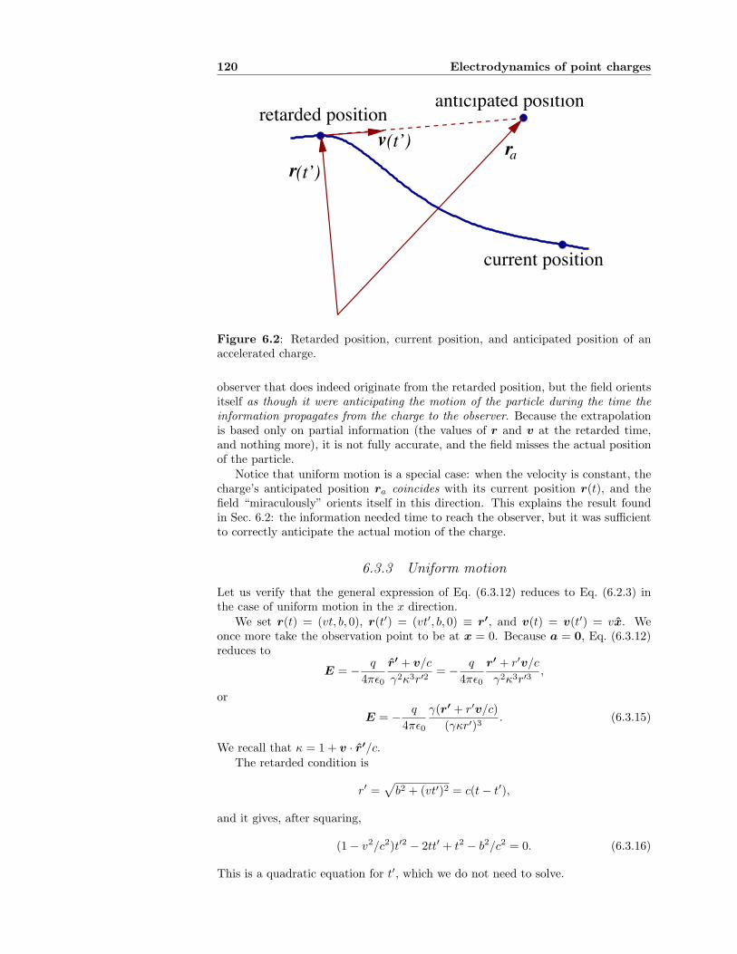
120 Electrodynamics of point charges
retarded position
r(t’)
v r(t’)a
current position
anticipated position
Figure 6.2: Retarded position, current position, and anticipated position of anaccelerated charge.
observer that does indeed originate from the retarded position, but the field orientsitself as though it were anticipating the motion of the particle during the time theinformation propagates from the charge to the observer. Because the extrapolationis based only on partial information (the values of r and v at the retarded time,and nothing more), it is not fully accurate, and the field misses the actual positionof the particle.
Notice that uniform motion is a special case: when the velocity is constant, thecharge’s anticipated position ra coincides with its current position r(t), and thefield “miraculously” orients itself in this direction. This explains the result foundin Sec. 6.2: the information needed time to reach the observer, but it was sufficientto correctly anticipate the actual motion of the charge.
6.3.3 Uniform motion
Let us verify that the general expression of Eq. (6.3.12) reduces to Eq. (6.2.3) inthe case of uniform motion in the x direction.
We set r(t) = (vt, b, 0), r(t′) = (vt′, b, 0) ≡ r′, and v(t) = v(t′) = vx. Weonce more take the observation point to be at x = 0. Because a = 0, Eq. (6.3.12)reduces to
E = −q
4πϵ0
r′ + v/c
γ2κ3r′2= −
q
4πϵ0
r′ + r′v/c
γ2κ3r′3,
or
E = −q
4πϵ0
γ(r′ + r′v/c)
(γκr′)3. (6.3.15)
We recall that κ = 1 + v · r′/c.The retarded condition is
r′ =0
b2 + (vt′)2 = c(t − t′),
and it gives, after squaring,
(1 − v2/c2)t′2 − 2tt′ + t2 − b2/c2 = 0. (6.3.16)
This is a quadratic equation for t′, which we do not need to solve.
6.3 Fields of an arbitrarily moving charge 121
The numerator of Eq. (6.3.15) involves the vector r′ + r′v/c. Its x componentis vt′ + r′v/c = vt′ + c(t − t′)v/c = vt, and this vector therefore coincides with r.In the denominator we have (γκr′)2 raised to the power 3/2. This is
(γκr′)2 = γ2(r′ + v · r′/c)2
= γ2(r′ + v2t′/c)2
= γ2c2(t − t′ + v2t′/c2)2
= γ2c2(t − t′/γ2)2
= c2(γ2t2 − 2tt′ + t′2/γ2).
We now use Eq. (6.3.16) to eliminate t′ and obtain
(γκr′)2 = c2'
b2/c2 + γ2t2(1 − 1/γ2)(
= b2 + γ2v2t2.
Substituting these results into Eq. (6.3.15) gives
E = −q
4πϵ0
γr(t)
(b2 + γ2v2t2)3/2, (6.3.17)
the same statement as Eq. (6.2.3).
6.3.4 Summary
The scalar and vector potentials of a point charge in arbitrary motion described bythe position vector r(t) are given by the Lienard-Wiechert expressions
Φ(t,x) =q
4πϵ0
3
1
κR
4
ret
(6.3.18)
and
A(t,x) =qµ0
4π
3
v
κR
4
ret
, (6.3.19)
where R(t′) = x − r(t′), R = |R|, R = R/R,
κ = 1 − v(t′) · R(t′)/c, (6.3.20)
and where t′ is determined by the retarded condition
|x − r(t′)| = c(t − t′). (6.3.21)
The electric field is
E(t,x) =q
4πϵ0
3
R − v/c
γ2κ3R2+
R ×'
(R − v/c) × a(
κ3c2R
4
ret
, (6.3.22)
and the magnetic field is
B =1
c
'
R(
ret× E. (6.3.23)
Both fields are naturally decomposed into velocity (bound) fields that decay as1/R2, and acceleration (radiative) fields that decay as 1/R.
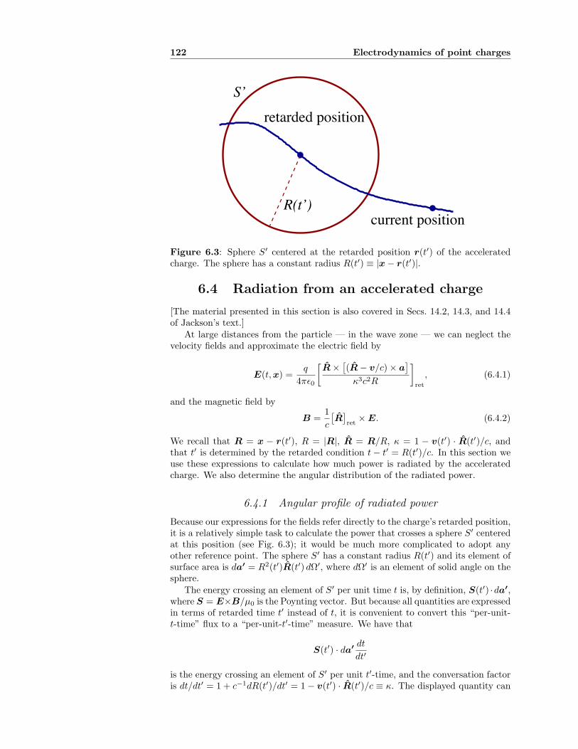
122 Electrodynamics of point charges
current positionR(t’)
S’
retarded position
Figure 6.3: Sphere S′ centered at the retarded position r(t′) of the acceleratedcharge. The sphere has a constant radius R(t′) ≡ |x − r(t′)|.
6.4 Radiation from an accelerated charge
[The material presented in this section is also covered in Secs. 14.2, 14.3, and 14.4of Jackson’s text.]
At large distances from the particle — in the wave zone — we can neglect thevelocity fields and approximate the electric field by
E(t,x) =q
4πϵ0
3
R ×'
(R − v/c) × a(
κ3c2R
4
ret
, (6.4.1)
and the magnetic field by
B =1
c
'
R(
ret× E. (6.4.2)
We recall that R = x − r(t′), R = |R|, R = R/R, κ = 1 − v(t′) · R(t′)/c, andthat t′ is determined by the retarded condition t − t′ = R(t′)/c. In this section weuse these expressions to calculate how much power is radiated by the acceleratedcharge. We also determine the angular distribution of the radiated power.
6.4.1 Angular profile of radiated power
Because our expressions for the fields refer directly to the charge’s retarded position,it is a relatively simple task to calculate the power that crosses a sphere S′ centeredat this position (see Fig. 6.3); it would be much more complicated to adopt anyother reference point. The sphere S′ has a constant radius R(t′) and its element ofsurface area is da′ = R2(t′)R(t′) dΩ′, where dΩ′ is an element of solid angle on thesphere.
The energy crossing an element of S′ per unit time t is, by definition, S(t′) ·da′,where S = E×B/µ0 is the Poynting vector. But because all quantities are expressedin terms of retarded time t′ instead of t, it is convenient to convert this “per-unit-t-time” flux to a “per-unit-t′-time” measure. We have that
S(t′) · da′dt
dt′
is the energy crossing an element of S′ per unit t′-time, and the conversation factoris dt/dt′ = 1 + c−1dR(t′)/dt′ = 1 − v(t′) · R(t′)/c ≡ κ. The displayed quantity can
6.4 Radiation from an accelerated charge 123
therefore be expressed as S(t′) · R(t′)R2(t′)κ dΩ′, which is a definition for dP ′ =(dP ′/dΩ′) dΩ′. We have arrived at
dP ′
dΩ′= κR2S · R (6.4.3)
= energy crossing an element of S′
per unit t′-time and unit solid angle.
Because it is understood that all quantities refer to the retarded time t′, we nolonger have a need for the redundant notation [ ]ret. Integrating Eq. (6.4.3) overdΩ′ gives the total power crossing S′. Integrating this over dt′ (which involvesdisplacing S′ in response to the particle’s motion during integration) returns thetotal energy radiated by the charge.
The Poynting vector is given by
S =1
µ0E × B =
1
µ0cE × (R × E) =
1
µ0c|E|2R,
because E is orthogonal to R. This gives
dP ′
dΩ′=
1
µ0cκR2|E|2 =
1
µ0c
q2
(4πϵ0)2
+
+R × [(R − v/c) × a]+
+
2
κ5c4,
ordP ′
dΩ′=
µ0q2
(4π)2c
+
+R × [(R − v/c) × a]+
+
2
κ5. (6.4.4)
The general expression for the angular profile is complicated, and it depends on theindividual directions of v, a, and R. To gain insight into this it will help to look atspecific simple situations; we shall do so in the following subsections. To ease thenotation we shall now agree to drop the primes on dP ′/dΩ′.
6.4.2 Slow motion: Larmor formula
Our first special case will be the limit v ≪ c. In this slow-motion approximationwe can neglect v/c in front of R in Eq. (6.4.4), and also set κ ≃ 1. We then have
dP
dΩ≃
µ0q2
(4π)2c
+
+R × (R × a)+
+
2
≃µ0q2
(4π)2c
+
+a − (a · R)R+
+
2
≃µ0q2
(4π)2c
1
|a|2 − (a · R)22
.
If θ denotes the angle between the vectors a and R, then |a|2 − (a · R)2 = |a|2(1−cos2 θ) = |a|2 sin2 θ, and we finally obtain
dP
dΩ≃
µ0
(4π)2c
%
q|a|&2
sin2 θ. (6.4.5)
This expression could have been derived on the basis of the electric-dipole ap-proximation of Sec. 5.4. According to the results of that section, in particularEq. (5.4.22), the angular profile of radiation produced by a slowly-moving source isgiven by
dP
dΩ=
µ0
(4π)2c|p|2 sin2 Θ,
124 Electrodynamics of point charges
where p is the dipole moment of the charge distribution, and Θ the angle betweenthe vectors r ≡ x/|x| and p. Here p = qr(t), so that p = qa. And because thesphere S′ is centered on the particle, the vector R plays the same role as r, so thatΘ ≡ θ. The electric-dipole approximation therefore produces the same result as inEq. (6.4.5).
Integration of dP/dΩ over all angles yields
P ≃µ0
6πc
%
q|a|&2
. (6.4.6)
This result is known as Larmor’s formula.
6.4.3 Linear motion
In this subsection we no longer restrict the size of v/c, but we assume that v and aare pointing in the same direction. This condition might hold at all times, but it issufficient to assume that it holds only momentarily. At this moment the particle ismoving on a straight line. We now let θ be the angle between R and the commondirection of v and a.
We have that v × a = 0, so Eq. (6.4.4) becomes
dP
dΩ=
µ0q2
(4π)2c
+
+R × (R × a)+
+
2
κ5.
We already know that |R×(R×a)|2 = |a|2 sin2 θ, and we recall that κ = 1−v·R/c =1 − v cos θ/c. Substituting these results gives
dP
dΩ=
µ0
(4π)2c
%
q|a|&2 sin2 θ
(1 − v cos θ/c)5. (6.4.7)
For v/c ≪ 1 this reproduces the sin2 θ behaviour encountered in the precedingsubsection. For v/c approaching unity, however, the angular profile is stronglymodified — it tips forward in the direction of v (θ = 0), and the power radiatedat small angles is very large (see Fig. 6.4). For such values of v/c, the radiation isbeamed in the forward direction.
The angular function is
f =sin2 θ
(1 − v cos θ/c)5. (6.4.8)
Differentiating with respect to µ ≡ cos θ and putting the result to zero indicatesthat the maximum of the distribution is at the value of µ that solves (3v/c)µ2 +2µ− 5v/c = 0. So most of the radiation is emitted at angles close to θmax, which isdetermined by
cos θmax =
0
1 + 15(v/c)2 − 1
3(v/c). (6.4.9)
For v/c ≪ 1, this expression is well approximated by cos θmax ≃ 52 (v/c)− 75
8 (v/c)3+· · ·, and θmax ≃ π/2: most of the radiation is emitted in the directions transverseto v. This is the usual nonrelativistic situation. For v/c close to unity, however, sothat γ ≫ 1, Eq. (6.4.9) is well approximated by cos θmax ≃ 1− 1
8γ−2− 43512γ−4 + · · ·,
and θmax is very small: most of the radiation is emitted in the forward direction.For such small angles we have cos θmax = 1 − 1
2θ2max + · · ·, and this gives us the
approximate relation
θmax ≃1
2γ, γ ≫ 1. (6.4.10)
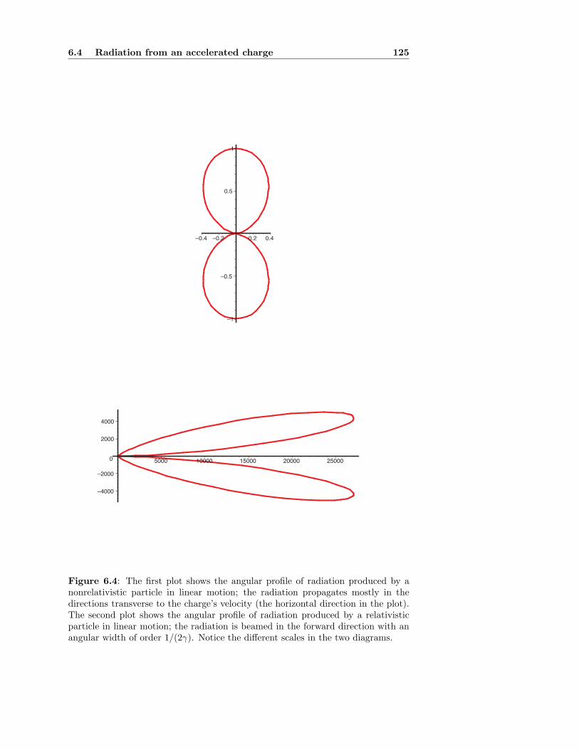
6.4 Radiation from an accelerated charge 125
–1
–0.5
0.5
1
–0.4 –0.2 0.2 0.4
–4000
–2000
0
2000
4000
5000 10000 15000 20000 25000
Figure 6.4: The first plot shows the angular profile of radiation produced by anonrelativistic particle in linear motion; the radiation propagates mostly in thedirections transverse to the charge’s velocity (the horizontal direction in the plot).The second plot shows the angular profile of radiation produced by a relativisticparticle in linear motion; the radiation is beamed in the forward direction with anangular width of order 1/(2γ). Notice the different scales in the two diagrams.
126 Electrodynamics of point charges
This is the statement that when the charge moves with a highly relativistic speed,the radiation is strongly beamed in the direction of the velocity vector.
The total power radiated is obtained by integrating Eq. (6.4.7) with respect todΩ = sin θ dθdφ. We have
P =µ0
(4π)2c
%
q|a|&2
2π
! π
0
sin3 θ dθ
(1 − v cos θ/c)5,
and the integral evaluates to 43γ6. The final answer is therefore
P =µ0
6πc
%
q|a|&2
γ6. (6.4.11)
This generalizes the Larmor formula of Eq. (6.4.6). It is instructive to express thisin terms of the force acting on the particle. This force is F = dp/dt, where p = mγvis the particle’s relativistic momentum. For linear motion in the x direction we havepx = mv/(1 − v2/c2)1/2 and
dpx
dt=
ma
(1 − v2/c2)1/2+
(mv)(v/c2)a
(1 − v2/c2)3/2=
ma
(1 − v2/c2)3/2.
This result can be expressed as F = mγ3a, and Eq. (6.4.11) becomes
P =µ0
6πc
"
q|F |m
#2
. (6.4.12)
This is the total power radiated by a charge in instantaneous linear motion.
6.4.4 Circular motion
We now take a and v to be orthogonal vectors. This condition might hold at alltimes, but it is sufficient to assume that it holds only momentarily. At this momentthe particle’s motion is circular. For concreteness we let a be directed along the xaxis, and v points in the z direction. We let the angles (θ,φ) give the direction ofthe vector R relative to this set of axes. We therefore have a = ax, v = vz, and
R = sin θ cos φ x + sin θ sinφ y + cos θ z.
According to this, v · R = v cos θ, a · R = a sin θ cos φ, κ = 1 − v cos θ/c, and
R ×'
(R − v/c) × a(
= (R · a)(R − v/c) − R · (R − v/c)a
= (R · a)(R − v/c) − κa.
The squared norm of this vector is
+
+R × [(R − v/c) × a]+
+
2= (R · a)2(R − v/c) · (R − v/c)
− 2κ(R · a)(R − v/c) · a + κ2a2
= (R · a)2(1 − 2R · v/c + v2/c2 − 2κ) + κ2a2
= −(R · a)2(1 − v2/c2) + κ2a2
= κ2a2
3
1 −(R · a)2
κ2γ2
4
.
Substituting this result into Eq. (6.4.4) gives
dP
dΩ=
µ0
(4π)2c
q2a2
κ3
3
1 −(R · a)2
κ2γ2
4
,
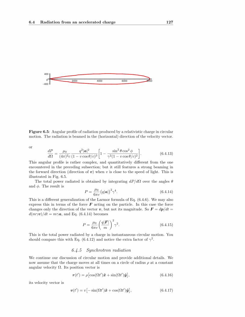
6.4 Radiation from an accelerated charge 127
–4000
400
2000 4000 6000 8000
Figure 6.5: Angular profile of radiation produced by a relativistic charge in circularmotion. The radiation is beamed in the (horizontal) direction of the velocity vector.
ordP
dΩ=
µ0
(4π)2c
q2|a|2
(1 − v cos θ/c)3
3
1 −sin2 θ cos2 φ
γ2(1 − v cos θ/c)2
4
. (6.4.13)
This angular profile is rather complex, and quantitatively different from the oneencountered in the preceding subsection; but it still features a strong beaming inthe forward direction (direction of v) when v is close to the speed of light. This isillustrated in Fig. 6.5.
The total power radiated is obtained by integrating dP/dΩ over the angles θand φ. The result is
P =µ0
6πc
%
q|a|&2
γ4. (6.4.14)
This is a different generalization of the Larmor formula of Eq. (6.4.6). We may alsoexpress this in terms of the force F acting on the particle. In this case the forcechanges only the direction of the vector v, but not its magnitude. So F = dp/dt =d(mγv)/dt = mγa, and Eq. (6.4.14) becomes
P =µ0
6πc
"
q|F |m
#2
γ2. (6.4.15)
This is the total power radiated by a charge in instantaneous circular motion. Youshould compare this with Eq. (6.4.12) and notice the extra factor of γ2.
6.4.5 Synchrotron radiation
We continue our discussion of circular motion and provide additional details. Wenow assume that the charge moves at all times on a circle of radius ρ at a constantangular velocity Ω. Its position vector is
r(t′) = ρ'
cos(Ωt′)x + sin(Ωt′)y(
, (6.4.16)
its velocity vector is
v(t′) = v'
− sin(Ωt′)x + cos(Ωt′)y(
, (6.4.17)
128 Electrodynamics of point charges
where v = Ωρ, and its acceleration vector is
a(t′) = −vΩ'
cos(Ωt′)x + sin(Ωt′)y(
. (6.4.18)
We wish to calculate the electric field that would be measured by a detector situatedfar away, in the wave zone. We place this detector on the y axis, at position x = ry,and we assume that r ≫ ρ.
The wave-zone electric field is given by Eq. (6.4.1), which we first evaluate asa function of retarded time t′. The relation between t′ and true time t is given byEq. (6.4.20). It is useful to recall that t′ is time measured by a clock that moveswith the charged particle, while t is time measured by a clock attached to thedetector. As we shall see, these measurements of time differ substantially when v iscomparable to c, and this leads to an interesting modulation of the electromagneticwave.
We use the condition r ≫ ρ to calculate E approximately. We shall needsome level of precision in the calculation of t(t′), because it is this function whichdetermines the phasing of the electric field. A much cruder approximation willsuffice when calculating the field’s amplitude.
Working to first order in ρ/r, it is easy to see that the length of the vectorR ≡ x − r(t′) is given by R(t′) = r − ρ sin Ωt′. Equation (6.3.21) then givest = t′ + r/c − (ρ/c) sin Ωt′, or
Ω(t − r/c) = Ωt′ −v
csin Ωt′. (6.4.19)
This gives the relationship between t − r/c, the retarded time measured at thedetector, and t′, the time measured at the particle. From this it follows that
κ =dt
dt′= 1 −
v
ccos Ωt′. (6.4.20)
We see that κ will deviate strongly from 1 when v is close to the speed of light andwhen | cos Ωt′| is close to unity.
To perform the remaining calculations we allow ourselves to neglect all termslinear in ρ/r. We take R = y,
R − v/c = (v/c) sin(Ωt′)x −'
1 − (v/c) cos(Ωt′)(
y,
and R× (R−v/c)×a = −vΩ(v/c− cos Ωt′)x. Substituting all this into Eq. (6.4.1)gives E = Ex, with
E = −q
4πϵ0
vΩ
c2r
v/c − cos Ωt′
[1 − (v/c) cos Ωt′]3. (6.4.21)
The electric field can be expressed in terms of detector time t by inverting Eq. (6.4.19).Its behaviour is displayed in Fig. 6.6 for selected values of γ = [1− (v/c)2]−1/2. Theplots reveal that for γ moderately larger than unity, the wave deviates strongly froma simple sinusoid. The phase modulations which originate from the discrepancy be-tween t and t′ produce a wave that is characterized by two distinct timescales: along one associated with the rotational frequency Ω, and a short one associatedwith the pulse duration. The frequency spectrum of the radiation is presented inFig. 6.7. These plots show that in the relativistic regime, the radiation is carriedby a large number of harmonics of the fundamental frequency Ω; as γ increases thedominant harmonic is shifted to higher frequencies.
To understand these features it is helpful to consider the extreme relativisticregime, in which γ ≫ 1. In this regime the basic mechanism behind the narrowingof the pulses is very easy to identify: When v/c → 1 the denominator of Eq. (6.4.21)
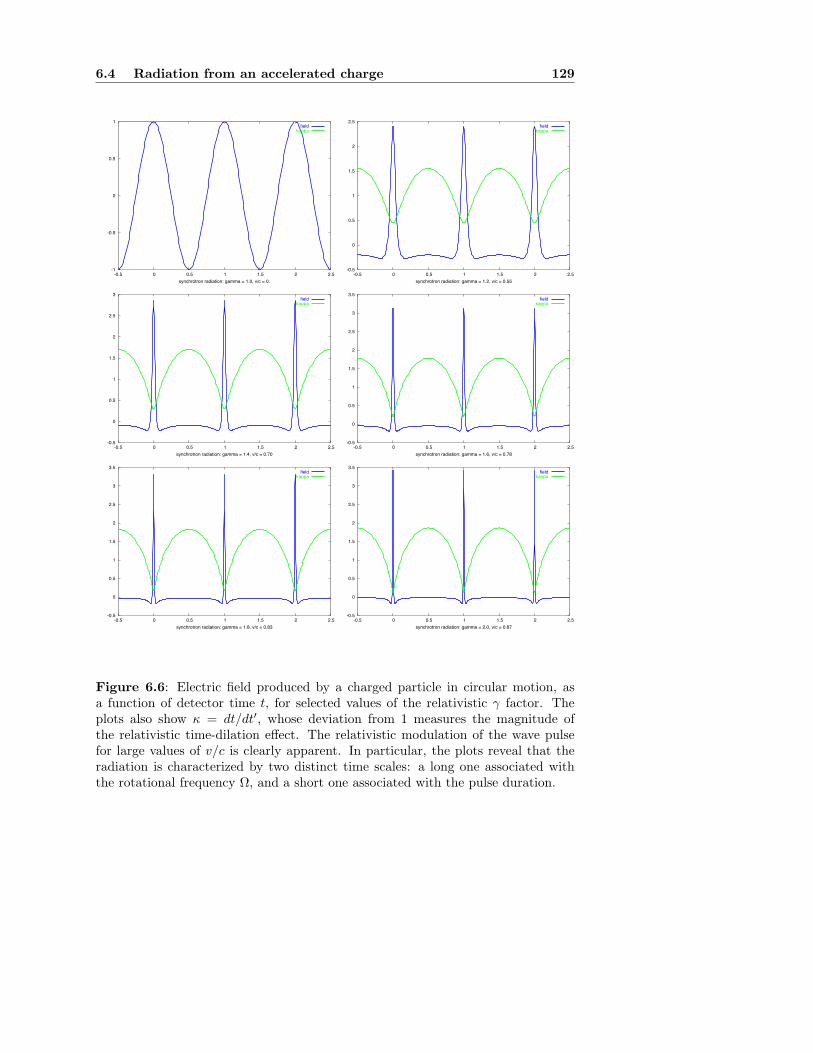
6.4 Radiation from an accelerated charge 129
-1
-0.5
0
0.5
1
-0.5 0 0.5 1 1.5 2 2.5synchrotron radiation: gamma = 1.0, v/c = 0.
fieldkappa
-0.5
0
0.5
1
1.5
2
2.5
-0.5 0 0.5 1 1.5 2 2.5synchrotron radiation: gamma = 1.2, v/c = 0.55
fieldkappa
-0.5
0
0.5
1
1.5
2
2.5
3
-0.5 0 0.5 1 1.5 2 2.5synchrotron radiation: gamma = 1.4, v/c = 0.70
fieldkappa
-0.5
0
0.5
1
1.5
2
2.5
3
3.5
-0.5 0 0.5 1 1.5 2 2.5synchrotron radiation: gamma = 1.6, v/c = 0.78
fieldkappa
-0.5
0
0.5
1
1.5
2
2.5
3
3.5
-0.5 0 0.5 1 1.5 2 2.5synchrotron radiation: gamma = 1.8, v/c = 0.83
fieldkappa
-0.5
0
0.5
1
1.5
2
2.5
3
3.5
-0.5 0 0.5 1 1.5 2 2.5synchrotron radiation: gamma = 2.0, v/c = 0.87
fieldkappa
Figure 6.6: Electric field produced by a charged particle in circular motion, asa function of detector time t, for selected values of the relativistic γ factor. Theplots also show κ = dt/dt′, whose deviation from 1 measures the magnitude ofthe relativistic time-dilation effect. The relativistic modulation of the wave pulsefor large values of v/c is clearly apparent. In particular, the plots reveal that theradiation is characterized by two distinct time scales: a long one associated withthe rotational frequency Ω, and a short one associated with the pulse duration.
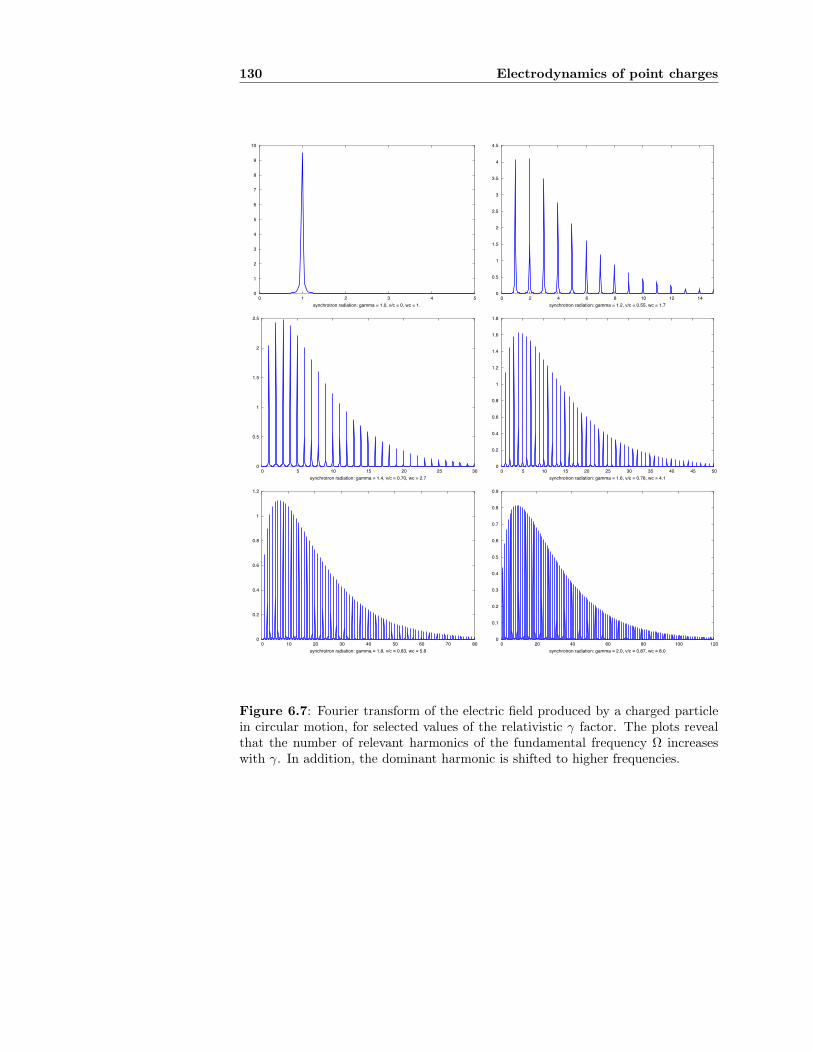
130 Electrodynamics of point charges
0
1
2
3
4
5
6
7
8
9
10
0 1 2 3 4 5synchrotron radiation: gamma = 1.0, v/c = 0, wc = 1.
0
0.5
1
1.5
2
2.5
3
3.5
4
4.5
0 2 4 6 8 10 12 14synchrotron radiation: gamma = 1.2, v/c = 0.55, wc = 1.7
0
0.5
1
1.5
2
2.5
0 5 10 15 20 25 30synchrotron radiation: gamma = 1.4, v/c = 0.70, wc = 2.7
0
0.2
0.4
0.6
0.8
1
1.2
1.4
1.6
1.8
0 5 10 15 20 25 30 35 40 45 50synchrotron radiation: gamma = 1.6, v/c = 0.78, wc = 4.1
0
0.2
0.4
0.6
0.8
1
1.2
0 10 20 30 40 50 60 70 80synchrotron radiation: gamma = 1.8, v/c = 0.83, wc = 5.8
0
0.1
0.2
0.3
0.4
0.5
0.6
0.7
0.8
0.9
0 20 40 60 80 100 120synchrotron radiation: gamma = 2.0, v/c = 0.87, wc = 8.0
Figure 6.7: Fourier transform of the electric field produced by a charged particlein circular motion, for selected values of the relativistic γ factor. The plots revealthat the number of relevant harmonics of the fundamental frequency Ω increaseswith γ. In addition, the dominant harmonic is shifted to higher frequencies.
6.4 Radiation from an accelerated charge 131
approaches zero whenever cos Ωt′ = 1, which happens whenever Ωt′ is a multiple of2π. Most of the radiation is therefore emitted during a very short portion of theparticle’s orbit, just as the particle crosses the x axis in the positive sense. Thisradiation is strongly beamed in the forward direction, and it travels along the yaxis toward the detector. During the remaining portion of the orbit little radiationis emitted, and the detector must wait for the completion of a full orbit beforereceiving the next pulse.
To express these ideas mathematically we write v/c = 1− 12γ−2+O(γ−4) and we
approximate sinΩt′ ≃ Ωt′ and cos Ωt′ ≃ 1 − 12 (Ωt′)2. From Eq. (6.4.20) we obtain
κ ≃1
2γ2
1
1 + (γΩt′)22
,
which shows that κ is small (of order γ−2 ≪ 1) for a duration of order (γΩ)−1 interms of particle time t′. We also obtain
v/c − cos Ωt′ ≃ −1
2γ2
1
1 − (γΩt′)22
,
and Eq. (6.4.21) reduces to
E ≃q
4πϵ0
vΩ
c2r4γ4 1 − (γΩt′)2
[1 + (γΩt′)2]3. (6.4.22)
Again, this shows that in terms of particle time t′, the radiation is “on” for aduration of order (γΩ)−1.
To see how long the pulse lasts in terms of detector time t, we approximateEq. (6.4.19) as Ω(t − r/c) ≃ 1
2γ−2Ωt′, which gives
γΩt′ ≃ 2γ3Ω(t − r/c). (6.4.23)
This relation reveals that the pulse duration, as measured by a clock attached tothe detector (and as displayed in Fig. 6.6) is given by
∆tpulse ∼1
γ3Ω. (6.4.24)
It is reduced by a factor γ−3 ≪ 1 relative to the orbital timescale associated withthe angular velocity Ω. As a consequence, the characteristic frequency ωc of theradiation is shifted relative to the fundamental frequency Ω. It is given by ωc ∼ γ3Ω,and the displacement of the spectrum toward higher frequencies when γ increasesis seen very clearly in Fig. 6.7.
6.4.6 Extremely relativistic motion
To conclude this section we note that at any point on the arbitrary trajectory of apoint charge, the applied force can be decomposed into a component that is parallelto the velocity vector v, and a component F⊥ that is perpendicular to it (F⊥ ·v = 0).When the motion is extremely relativistic, γ ≫ 1 and the total power emitted bythe particle is well approximated by Eq. (6.4.15),
P =µ0
6πc
"
q|F⊥|m
#2
γ2.
The contribution from the parallel force is smaller by a factor of 1/γ2 ≪ 1, andit can be neglected. In this limit, therefore, the parallel force plays no role in theenergetics of the radiation.
132 Electrodynamics of point charges
6.5 Radiation reaction
[The material presented in this section is also covered in Secs. 16.1, 16.2, and 16.3of Jackson’s text.]
In Sec. 5.6 we saw that a classical electron orbiting a classical proton emitselectromagnetic radiation. As a result, the classical hydrogen atom loses energy ata rate determined by Larmor’s formula,
dE
dt= −P = −
µ0
6πc
%
q|a|&2
.
This loss of energy translates into a decrease in the electron’s orbital radius. Theorbit gradually shrinks, and the classical atom is unstable to the emission of elec-tromagnetic radiation.
It is natural to assume that the electron is subjected only to the electric fieldproduced by the proton. This picture, however, is incomplete: So long as theelectron feels only the proton’s Coulomb field, its motion must stay circular (or moregenerally, elliptical). The electron’s inspiraling motion cannot take place in thispicture, in contradiction with our previous description. We are forced to concludethat the proton’s electric field cannot be the only field acting on the electron. Theelectron must also be subjected to its own electric field. It is the electron’s self-fieldwhich provides the force that drives the electron’s inspiraling motion.
This conclusion is difficult to understand, because the electron’s own field di-verges at the electron’s position. How can it then produce a (presumably finite)radiation-reaction force that drives the inspiral? The answer is that the divergentpart of the electron’s self-field exerts no force — it just travels along with the elec-tron. The part of the self-field that is responsible for the radiation reaction is finite.
To figure out what this part is, let us ask what would happen if instead ofimposing outgoing-wave boundary conditions on our spherical-wave solutions toMaxwell’s equations, we were to impose incoming-wave boundary conditions. Inthis case we would have incoming waves bringing energy to the system instead ofoutgoing waves taking energy away. The atom’s energy would then increase, andthe electron would move out instead of in. We would, in fact, have a mirror image(more precisely, a time reversal) of the correct picture, and the radiation-reactionforce would be acting in the opposite direction (pushing the orbit out instead of in).
We can figure out which part of the electron’s field is producing the radiation-reaction force by examining what happens when we switch from outgoing-waveboundary conditions to incoming-wave boundary conditions. We will see that whilepart of the field is not affected by this switch, the remaining part changes sign.And we will see that while the unaffected part is infinite at the electron’s position,the remaining part is finite. It is this part of the field that is responsible for theradiation reaction.
Let us examine the vector potential first. The physical solution to Maxwell’sequations is the retarded solution,
A−(t,x) =µ0
4π
!
j(t − |x − x′|/c,x′)
|x − x′|d3x′,
where j is the electron’s current density. This describes waves that are properlyoutgoing in the wave zone. These waves remove energy from the system, and theradiation reaction drives the electron inward. An unphysical solution to Maxwell’sequations is the advanced solution,
A+(t,x) =µ0
4π
!
j(t + |x − x′|/c,x′)
|x − x′|d3x′,
6.5 Radiation reaction 133
and this describes waves that are incoming in the wave zone. These waves bringenergy to the system, and the radiation reaction drives the electron outward. Toisolate the part of the (retarded) vector potential that is responsible for the radia-tion reaction, we must examine both solutions simultaneously, and determine whatchanges when we choose one sign over the other.
We want to evaluate A± near the electron, in the near zone. We can thereforetake |x − x′| to be small, and Taylor-expand the current density:
j(t ± |x − x′|/c) = j(t) ±|x − x′|
c
∂j
∂t(t) + · · · .
Relative to the leading term, the second term is of order (rc/tc)/c = vc/c, and weshall take this to be small — we are working under a slow-motion approximation.We have
A± =µ0
4π
!
j(t,x′)
|x − x′|d3x′ ±
µ0
4πc
d
dt
!
j(t,x′) d3x′ + · · · .
We see that the first term is the same irrespective of the choice of boundary con-ditions (outgoing waves versus incoming waves); it cannot, therefore, contribute toa radiation-reaction force. The second term, however, changes sign under a changeof boundary conditions, and the force it contributes will also change sign; this mustbe the vector potential’s contribution to the reaction-reaction force. Because theretarded solution provides the correct sign, we shall write
Arr(t,x) = −µ0
4πc
d
dt
!
j(t,x′) d3x′ + · · · , (6.5.1)
and we will see that the fields this potential generates produce the radiation-reactionforce that acts on the electron.
For the scalar potential we have the two solutions
Φ±(t,x) =1
4πϵ0
!
ρ(t ± |x − x′|/c,x′)
|x − x′|d3x′,
and we Taylor-expand the charge density:
ρ(t ± |x − x′|/c) = ρ(t) ±|x − x′|
c
∂ρ
∂t(t) +
|x − x′|2
2c2
∂2ρ
∂t2(t)
±|x − x′|3
6c3
∂3ρ
∂t3(t) + · · · .
This gives
Φ± =1
4πϵ0
3!
ρ(t,x′)
|x − x′|d3x′ ±
1
c
d
dt
!
ρ(t,x′) d3x′
+1
2c2
∂2
∂t2
!
ρ(t,x′)|x − x′| d3x′
±1
6c3
∂3
∂t3
!
ρ(t,x′)|x − x′|2 d3x′ + · · ·4
.
The first and third terms are insensitive to boundary conditions; they have nothingto do with radiation reaction. The second and fourth terms, on the other hand,change sign under a switch of boundary conditions, and they are associated withradiation reaction. The second term, however, vanishes by virtue of charge conser-vation, and we conclude that the radiation-reaction part of the scalar potential isgiven by (recall that c−2 = ϵ0µ0)
Φrr(t,x) = −µ0
4πc
1
6
∂3
∂t3
!
ρ(t,x′)|x − x′|2 d3x′ + · · · . (6.5.2)
134 Electrodynamics of point charges
Up to now the charge and current densities have been left unspecified, and ourconsiderations have been general: Eqs. (6.5.1) and (6.5.2) give the radiation-reactionpotentials for an arbitrary distribution of change and current. These expressionswill apply, in particular, to a point charge q if we set ρ(t,x′) = qδ(x′ − r(t)) andj(t,x′) = qv(t)δ(x′−r(t)), where v = dr/dt. Substituting this into our expressionsfor the potentials returns
Φrr(t,x) = −µ0
4πc
q
6
∂3
∂t3+
+x − r(t)+
+
2
and
Arr(t,x) = −µ0
4πcq
d
dtv(t).
We have |x−r|2 = (x−r) · (x−r), and differentiating once with respect to t gives−2(x−r)·v. Differentiating once more gives −2(x−r)·a+2v ·v, and differentiatinga third time yields −2(x−r) · a+2v ·a+4v ·a = −2(x−r) · a+6v ·a. We finallyarrive at
Φrr(t,x) =µ0
4πcq
3
1
3(x − r) · a − v · a
4
(6.5.3)
andArr(t,x) = −
µ0
4πcqa. (6.5.4)
Here we have defined a = dv/dt and a = da/dt. These are the radiation-reactionpotentials acting on a point charge q moving on a trajectory r(t).
The radiation-reaction part of the electric field is given by
Err = −∂Arr
∂t− ∇Φrr =
µ0
4πcq
"
a −1
3a
#
,
orErr =
µ0
6πcqa. (6.5.5)
Because Arr does not actually depend on x, we also have
Brr = 0. (6.5.6)
The radiation-reaction force is therefore Frr = qErr, or
Frr =µ0
6πcq2a. (6.5.7)
This force acts on the point charge, and it originates from the charge’s own electricfield!
It is easy to verify that the radiation-reaction force does negative work on theparticle and takes energy away from it. As the charge moves with velocity v theforce does work at a rate
W = Frr · v =µ0
6πcq2a · v.
We write
a · v =d
dt(a · v) − |a|2,
and we average W over a time interval T . This gives
⟨W ⟩ ≡1
T
! T
0W dt
=µ0
6πcq2
3
1
T
! T
0
d
dt(a · v) dt −
1
T
! T
0|a|2 dt
4
=µ0
6πcq2
3
1
T(a · v)
+
+
+
T
0−
:
|a|2;
4
.
6.6 Problems 135
Supposing now that the motion is periodic with period T (as it would be in the caseof atomic motion), or else that it begins and ends with a vanishing acceleration, wemay discard the boundary terms and obtain
⟨W ⟩ = −µ0
6πcq2
:
|a|2;
= −⟨P ⟩, (6.5.8)
where P is the power radiated by the point charge, as given by the Larmor formulaof Eq. (6.4.6). The work done by the radiation-reaction force therefore matches theenergy taken away by electromagnetic radiation, and we have energy conservation.(It is noteworthy that this statement holds only on the average.)
We have a complete resolution of the paradox stated at the beginning of thissection. The electron’s own field, or at least the finite part that is sensitive to thechoice of boundary conditions, acts on the electron and prevents it from keeping itscircular motion. (Indeed, it is easy to check that for a circular orbit, the radiation-reaction force of Eq. (6.5.7) points in the direction of −v and drives the orbitto a smaller radius.) Furthermore, the work done by this radiation-reaction forcematches the amount of energy taken away by the radiation, as it well should ifenergy is to be conserved in the process.
6.6 Problems
1. A point charge q moves on a circle of fixed radius a with an angular frequencyω(t) that changes slowly with time. (The time scale over which ω changes ismuch longer than the rotational period.) We take aω to be smaller than c,but we do not assume that it is much smaller than c; the charge has a Lorentzγ-factor that can be large compared with unity.
The charge emits electromagnetic radiation. It therefore loses energy andthis causes the angular frequency ω to change with time. You are asked toderive an equation for dω/dt and to express your result in terms of ω, a, andother relevant constants. (You may need to know that the charge’s relativisticenergy is E = γmc2, where m is the charge’s rest mass.)
2. (This problem is adapted from Jackson’s problem 14.12.) A charge q movesin simple harmonic motion along the z axis. Its position is given as a functionof t′ by z(t′) = z0 cos(ωt′), where z0 and ω are constants. It is assumed thatβ ≡ z0ω/c is fairly close to unity, so that the motion is relativistic.
a) Show that the time-averaged angular profile of the radiation is describedby
<
dP
dΩ
=
=µ0
32π2c(qz0ω
2)21 + (β/2)2 cos2 θ
(1 − β2 cos2 θ)7/2sin2 θ,
where θ is the angle from the z axis. The time average is defined by
⟨(· · ·)⟩ ≡ T−1* T0 (· · ·) dt′, where T ≡ 2π/ω is the period.
b) Produce a parameteric plot of the angular function for β = 0.95. Commenton its appearance in view of the beaming effect discussed in Sec. 6.3.3.
3. A charge q moves on a trajectory described by z(t′) =0
b2 + (ct′)2, where bis a constant. The particle comes in from infinity, it turns around at z = bwhen t′ = 0, and it eventually returns to infinity.
Calculate P , the total power emitted by the particle. Show in particular thatthis does not depend on time t′.
136 Electrodynamics of point charges
4. (This problem is adapted from Jackson’s problem 14.7.) A nonrelativisticparticle of charge q, mass m, and initial speed v is incident on a fixed chargeQ with an impact parameter b that is large enough to ensure that the particle’sdeflection in the course of the collision is very small.
Calculate the total energy radiated by the particle. Because the deflectionangle is so small, it is sufficient to assume that the particle’s trajectory is astraight line and that its velocity vector is constant. But this approximationmust be introduced only after you have calculated the particle’s acceleration.