electromagnetic modelling including the ferromagnetic core · electromagnetic transformer modelling...
TRANSCRIPT

Electromagnetic transformer modelling including the
ferromagnetic core
David Ribbenfjärd
Doctoral thesis in Electrical Systems
Stockholm, Sweden 2010

TRITA-EE 2010:023 ISSN 1653-5146 ISBN 978-91-7415-674-4
Elektroteknisk teori och konstruktion
Kungliga Tekniska Högskolan SE-100 44 Stockholm
SWEDEN
Akademisk avhandling som med tillstånd av Kungliga Tekniska Högskolan framläggs till offentlig granskning för avläggande av teknologie doktorsexamen torsdagen den 17 juni 2010 klockan 13.15 i sal F3, Kungliga Tekniska Högskolan, Lindstedtsvägen 26, Stockholm.
© David Ribbenfjärd, 2010
Tryck: Universitetsservice US-AB

To Sara, Tilda and Signe


Abstract
In order to design a power transformer it is important to understand its internal electromagnetic behaviour. That can be obtained by measurements on physical transformers, analytical expressions and computer simulations. One benefit with simulations is that the transformer can be studied before it is built physically and that the consequences of changing dimensions and parameters easily can be assesed.
In this thesis a time-domain transformer model is presented. The model includes core phenomena as magnetic static hysteresis, eddy current and excess losses. Moreover, the model comprises winding phenomena as eddy currents, capacitive effects and leakage flux. The core and windings are first modelled separately and then connected together in a composite transformer model. This results in a detailed transformer model.
One important result of the thesis is the feasibility to simulate dynamic magnetization including the inhomogeneous field distribution due to eddy currents in the magnetic core material. This is achieved by using a Cauer circuit combined with models for static and dynamic magnetization. Thereby, all magnetic loss components in the material can be simulated accurately. This composite dynamic magnetization model is verified through experiments showing very good correspondence with measurements.
Furthermore, the composite transformer model is verified through measurements. The model is shown to yield good correspondence with measurements in normal operation and non-normal operations like no-load, inrush current and DC-magnetization.
Keywords: Power transformer, hysteresis, dynamic hysteresis, dynamic magnetization, eddy currents, excess losses, leakage flux, winding model, core model, magnetic measurements, magnetic materials

Acknowledgement
I would like to thank the following persons:
Prof. Göran Engdahl, my supervisor for guidance in the project, interesting and productive discussions about transformers and especially magnetic materials. I am also grateful for the careful review of this thesis.
Prof. Roland Eriksson and Prof. Rajeev Thottappillil, former and present head of the department, respectively, for guidance in the project.
Dr. Dierk Bormann, secondary supervisor, for support and interesting discussion of transformer models.
Lic. Mattias Oscarsson, Lic. Héctor Latorre, Dr. Valentinas Dubickas and Dr. Mohsen Torabzadeh-Tari, former colleagues, for interesting discussions and friendship.
Thanks to Peter Lönn for technical support with computer hardware and software. Also thanks to Carin Norberg for administration support.
Thank to ABB Corporate Research for letting me use there lab for measurements and providing with test transformer. Thanks to Cogent Power Ltd, Surahammars Bruk, for providing and treating materials.
Finally thanks to my family, my wonderful wife Sara and my cute daughters Tilda and Signe for making me happy.


Contents
CHAPTER 1 INTRODUCTION ..................................................1
1.1 BACKGROUND.........................................................................1 1.2 AIM .........................................................................................2 1.3 OUTLINE OF THE THESIS..........................................................3 1.4 LIST OF PUBLICATIONS............................................................5
CHAPTER 2 TRANSFORMER BASICS ...................................7
2.1 OPERATION OF THE TRANSFORMER ........................................7 2.1.1 Basic principles ...............................................................7 2.1.2 Losses in transformers ...................................................10
2.2 LOSSES IN THE CORE .............................................................11 2.2.1 Properties of magnetic materials ...................................12
2.2.1.1 Magnetic domains ................................................................... 12 2.2.1.2 Basic relations ......................................................................... 13 2.2.1.3 Hysteresis ................................................................................ 14 2.2.1.4 Reversible and irreversible processes ..................................... 16
2.2.2 Dynamic properties of magnetic materials ....................19 2.2.2.1 Classical eddy currents............................................................ 19 2.2.2.2 Excess loss............................................................................... 20 2.2.2.3 Total field ................................................................................ 21 2.2.2.4 Another description of dynamic magnetization...................... 25
2.2.3 Additional loss sources in real cores .............................25 2.3 LOSSES IN THE WINDING .......................................................26
2.3.1 Losses in the winding conductors..................................26 2.3.2 Other loss mechanisms in the windings.........................27
CHAPTER 3 WINDING MODEL .............................................29
3.1 MODELLING OF LOSSES IN CONDUCTORS..............................30 3.1.1 Analytical expression for eddy currents ........................31
3.1.1.1 Equivalent circuits................................................................... 36 3.1.1.2 Discussion ............................................................................... 37
3.2 MODELLING OF CAPACITIVE EFFECTS...................................37 3.2.1 Discussion .....................................................................40
3.3 MODELLING OF FLUX IN THE WINDING .................................40 3.3.1 Discussion .....................................................................42
CHAPTER 4 CORE MODEL ....................................................43
4.1 STATIC MAGNETIZATION MODEL ..........................................43 4.1.1 Bergqvist’s lag model....................................................43
4.1.1.1 One dimensional model........................................................... 44 4.1.1.2 Multi dimensional model ........................................................ 45
4.1.2 Modifications.................................................................47 4.1.2.1 Anhysteretic curve obtained from measurements................... 47 4.1.2.2 Anhysteretic curve as mathematical function ......................... 51 4.1.2.3 Improved curve modelling at high fields ................................ 54 4.1.2.4 Variable pinning strength........................................................ 56 4.1.2.5 Variable degree of reversibility............................................... 60 4.1.2.6 Modified play operator............................................................ 61
4.2 DYNAMIC MAGNETIZATION MODEL......................................63 4.2.1 Cauer circuits.................................................................63
4.2.1.1 Modelling method ................................................................... 64 4.2.1.2 Optimization of Cauer circuit at high frequencies .................. 69 4.2.1.3 The feasibility of studying the flux distribution along the cross-section of a magnetic material................................................................. 73
4.3 COMPOSITE MAGNETIZATION MODEL ...................................74 4.3.1 Discussion .....................................................................75
CHAPTER 5 COMPOSITE TRANSFORMER MODEL .......77
5.1 ONE PHASE............................................................................77 5.2 THREE PHASES ......................................................................78
CHAPTER 6 EXPERIMENTAL VERIFICATION.................81
6.1 CORE MODEL VERIFICATION .................................................81 6.1.1 Static measurements ......................................................82
6.1.1.1 Set-up ...................................................................................... 82 6.1.1.2 Major loops ............................................................................. 83 6.1.1.3 Minor loops ............................................................................. 84
6.1.2 Static simulations...........................................................85 6.1.2.1 Major loops ............................................................................. 86 6.1.2.2 Minor loops ............................................................................. 89 6.1.2.3 Discussion ............................................................................... 92

6.1.3 Dynamic measurements with controlled H-field ...........93 6.1.3.1 Set-up ...................................................................................... 93 6.1.3.2 Influence of cutting on the permeability ................................. 95 6.1.3.3 Measurements of stress-relief annealed materials .................. 97
6.1.4 Dynamic measurements with controlled B-field ...........99 6.1.5 Dynamic simulations with controlled H-field .............102
6.1.5.1 Simulation procedure ............................................................ 103 6.1.5.2 Simulations using Cauer circuits........................................... 103 6.1.5.3 Simulations using the classical eddy currents expression .... 106 6.1.5.4 Conclusions ........................................................................... 109
6.1.6 Dynamic simulations with controlled B-field..............109 6.1.6.1 Conclusions and discussion................................................... 119
6.1.7 Estimation of the frequency dependence of excess losses. .....................................................................................120
6.1.7.1 Discussion ............................................................................. 123 6.2 TRANSFORMER MODEL VERIFICATION................................123
6.2.1 Measurements..............................................................124 6.2.1.1 Normal operation .................................................................. 127 6.2.1.2 Non normal operation ........................................................... 127
6.2.2 Simulations ..................................................................127 6.2.2.1 Normal operation .................................................................. 133 6.2.2.2 Discussion ............................................................................. 136 6.2.2.3 No-load operation.................................................................. 136 6.2.2.4 Inrush current ........................................................................ 140 6.2.2.5 DC-magnetization ................................................................. 144 6.2.2.6 Short-circuit........................................................................... 147
6.2.3 Discussion ...................................................................147
CHAPTER 7 CONCLUSIONS AND FUTURE WORK........149
7.1 CONCLUSIONS.....................................................................149 7.2 FUTURE WORK ....................................................................150
APPENDIX I...................................................................................153
APPENDIX II .................................................................................162
APPENDIX III................................................................................167
APPENDIX IV................................................................................168
REFERENCES ...............................................................................171

LIST OF SYMBOLS......................................................................181
LIST OF ACRONYMS..................................................................183
Introduction Chapter 1
1
Chapter 1
Introduction
1.1 Background
Power transformers have been in use for over 120 years to day’s date [1] and are key components for transmission and distribution of electrical power. In a transformer, energy is transferred between two electrical circuits by magnetic coupling. The working principle of transformers is well-known; nevertheless, research on and development of design and materials are still taking place. The reason for this is that there is a vast amount of transformers in the electrical networks over the world and decreasing losses in the transformers means less expense for the network owners.
Power transformers are very large in size and expensive to manufacture. Therefore, models and computer simulations of transformers are saving both time and assets for the developers and manufacturers. Furthermore, by using computer models the risk of destroying the transformer during tests is reduced. In order to substitute real tests for simulations, the simulation models have to be highly detailed. This is since the internal operation of the transformer includes very complex electromagnetic behaviours. The causes for this are, e.g., the large number of conductors, the need for insulation between conductors, the potential difference between conductors and grounded parts and the magnetic core, respectively, etc. Especially the magnetic core introduces complex properties that are not present in electrical components without magnetic parts.
The importance of the core is highest at low frequencies whereas the winding is the more important part at high frequencies. This fact together with the complexity of transformers has resulted in that the describing models often have

Chapter 1 Introduction
2
been simplified. Moreover, this has usually been done by rather detailed modelling of the windings and coarse description of the core or vice versa. Therefore, there exists a wide variety of transformer models. A review of transformer models intended for low- and mid-frequency ranges is found in ref [2]. Below is listed a selection of references using models with different resolutions of the core models:
• Including magnetic saturation: Narang and Brierley [3] and Mork [4].
• Including magnetic saturation and hysteresis: Annakage et al [5].
• Including magnetic saturation, hysteresis and eddy currents: Dolinar et al. [6], Dallago et al. [7], Tarasiewicz et al. [8], Archer et al. [9], Chen and Neudorfer [10].
• Including magnetic saturation, hysteresis, eddy currents and excess losses: Chandrasena et al. [11], [12].
Furthermore, de Leon and Semlyen takes eddy currents and the eddy current shielding effect into account, however, they do not include magnetic saturation and hysteresis [13], [14], [15], [16], [17], [18].
Nevertheless, there is still a need for exact transformer models with high resolution of the core and winding.
1.2 Aim
The aim of this project is to develop models and methods that can be used in simulations and in the assembly of entire transformer models. The models shall include loss phenomena in both the core and the windings. Examples of phenomena to be included are:
• Magnetic static hysteresis
• Saturation of magnetic materials

Introduction Chapter 1
3
• Dynamic magnetization effects like eddy currents and excess loss in the core
• Eddy current shielding effect in both windings and core
• Eddy currents in the windings
• Capacitive effects in the windings
• Leakage flux
The goal is to create a transformer model with detailed descriptions of both the core and windings where all the above listed phenomena are included. Moreover, the model shall be built as a module and capable to be a part of a larger electrical network. The model itself shall be built up of smaller modules. Furthermore, these modules should be able to be used in other components and applications.
1.3 Outline of the thesis
Chapter 2 starts with a short summary of the operation of transformers. Then the origin of electromagnetic losses in the core and windings are described. Moreover, the magnetization processes and hysteresis in magnetic materials are described. Furthermore, the background to dynamic magnetization; eddy currents and excess losses are presented. Especially, Bertotti’s statistical loss model [19] for the excess losses is presented. Finally, loss phenomena in the windings are described.
Chapter 3 presents a winding model including an analytical expression for the eddy currents in the winding conductors. The approach originally derived by Perry [20], [21], [22] is described. The model also includes capacitive effects and leakage flux. The author’s contribution to this chapter is the incorporation of resistive and reactive components, comprising the eddy current losses, into an electrical network of the windings. Furthermore, the dividing of the winding space into different regions regarding the flux was performed by the author.
Chapter 1 Introduction
4
Chapter 4 introduces the core model, starting with the static magnetization model first proposed by Dr. Anders Bergqvist [23], [24], [25] . Then, some modifications of this static model are presented. Next, a dynamic magnetization model using Cauer circuits for modelling eddy currents and the statistical loss model for description of the excess losses is presented.
The author’s contribution to this chapter is the development of the logarithmical modification of mathematical function for creating anhysteretic curves. Furthermore, the variable pinning strength was developed by the author. The use of a variable degree of reversibility was proposed by the author; however, the mathematical derivations were developed by Prof. Engdahl. The measurement of an anhysteretic curve was initiated by Prof. Engdahl and performed by Dr. Sisir Nayak. The author contributed with support during measurements and data processing. The idea to use Bergqvist’s lag model together with the classical eddy current expression and Bertottis statistical loss theory was first initiated by Prof. Engdahl. The substitution of the classical eddy current expression for the Cauer circuits was initiated and performed by the author. The idea to optimize the regions in the Cauer circuits was first proposed by Prof. Engdahl. The parameter estimation procedure for Bergqvist’s lag model, which is presented in Appendix II, was developed by Dr. Bergqvist.
Chapter 5 demonstrates the composite one-phase and three-phase transformer models including the core and winding models.
Chapter 6 contains verifications of both the static and dynamic magnetization models for electrical steels. For the static condition, measured and simulated results of major and minor loops are shown. Moreover, the dynamic magnetization model is verified under two different magnetization conditions: with controlled H-field and controlled B-field, respectively. Also comparisons between the proposed Cauer circuit model and the classical eddy current model are shown.
In addition, the dynamic model is used for studying the frequency dependence of the excess losses.
This chapter also includes verification of the composite transformer model, including measurements and simulations. This model is verified under normal operation with different loads and non-normal operations like no-load, inrush current and DC-magnetization conditions.

Introduction Chapter 1
5
All measurements and simulations, except the measurements of the minor loops, have been performed by the author. The cutting of the electrical steels for verification of the dynamic magnetization model with controlled H-field was done by the author together with Dr. Arvid Broddefalk at Cogent Power Ltd. The stress-relief annealing of theses materials were performed by Dr. Broddefalk.
Chapter 7 concludes the thesis and proposes topics for future work.
1.4 List of publications
Some of the results in this thesis have been published in the publications below:
I. Austrin L., Ribbenfjärd D., Engdahl G. Simulation of a magnetic amplifier
circuit including hysteresis, IEEE Transactions on Magnetics, Vol. 41, No. 10, pp. 3994-3996,October 2005
II. Ribbenfjärd D., Engdahl G., Time-domain transformer model in Dymola,
Proceedings of 2nd International Conference “From Scientific Computing to Computational Engineering”, Athens, Greece, July 2006
III. Ribbenfjärd D., Engdahl G., Modeling of Dynamic Hysteresis with
Bergqvist's Lag Model, IEEE Transaction on Magnetics, Vol. 42, No. 10, pp. 3135-3137, October 2006
IV. Ribbenfjärd D., Engdahl G., Hysteresis Modeling Including Asymmetric
Domain Rotation, IEEE Transaction on Magnetics, Vol. 43, No. 4, pp. 1385-1388, April 2007
V. Ribbenfjärd D., Engdahl G., Optimization of the Geometrical Selection of
Subsections in Cauer Circuit Models of Laminated Magnetic Materials at High Frequencies, Proceedings of 13th Biennial IEEE Conference on Electromagnetic Field Computation, p. 337, Athens, Greece, May 2008
VI. Ribbenfjärd D., Engdahl G., Novel Method for Modelling of Dynamic
Hysteresis, IEEE Transaction on Magnetics, Vol. 44, No. 6, pp. 854-857, June 2008

Chapter 1 Introduction
6
VII. Tavakoli H., Bormann D., Ribbenfjärd D., Engdahl G., Comparison of a
Simple and a Detailed Model of Magnetic Hysteresis with Measurements on Electrical Steel, COMPEL, Vol. 28, No. 3, pp. 700-710, 2009
VIII. Ribbenfjärd D., Engdahl G., Study of Excess Loss Term in Ferromagnetic
Laminations using Cauer Circuits, Digests of 11th Joint MMM/InterMag Conference, p. 887, Washington, DC, USA, January 2010
Transformer basics Chapter 2
7
Chapter 2
Transformer basics
2.1 Operation of the transformer
2.1.1 Basic principles The operation of transformers bases on the electromagnetic induction principle. An electric current, I, in a winding wound around a core, induces a magnetic field, H, in that core. This is in accordance with the line integral form of Ampère’s law:
C
I=∫ iH dl (2.1)
Here, C is a closed curve and dl an infinitesimal element of C. The field gives rise to a magnetic flux, φ, and by use of magnetic materials, the flux is magnified. The line integral form of Faraday’s law states that
C
ddtϕ
=−∫ iE dl (2.2)
Here, E is an electric field enclosing the flux. This means that an alternating flux creates electric fields surrounding it.

Chapter 2 Transformer basics
8
For example, in a two-winding transformer as depicted in Fig 2.1, a voltage is applied to the primary winding which causes a current to flow in this winding. The current creates a magnetic flux in the core, according to Ampère’s law. The flux, in turn, induces voltages in both of the surrounding windings, according to Faraday’s law. In the primary winding the induced voltage has opposite polarity compared to the applied voltage. However, due to the losses in the core the induced voltage is slightly smaller than the applied. Therefore, a current corresponding to the difference between the applied and induced voltage, will flow.
In the secondary winding the induced voltage drives a current with opposite polarity with respect to the current in the primary winding. These currents induce opposing fluxes in the core, which however, never will be exactly equal in magnitude. This is due to the losses in core and windings.
Fig 2.1. Cross-sectional view of one leg of a two-winding transformer.

Transformer basics Chapter 2
9
Let us now consider the working principle of an ideal transformer, which would have no losses. If the secondary side is unloaded (no-load condition) there is no current in this winding and the ratio between the voltages in the windings, U1 and U2 respectively, is:
1 1
2 2
U NU N
= (2.3)
Here, N1 and N2 are the number of turns in the windings, respectively.
In a load condition the ratio between the currents in the windings, I1 and I2, respectively, is:
1 2
2 1
I NI N= (2.4)
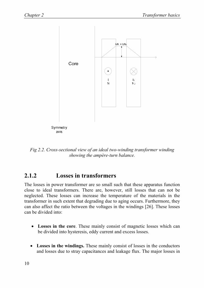
In Fig 2.2 an ampère-turn diagram of an ideal two-winding transformer is shown. The height of the diagram represents the current integral along the radial axis. Traversing along this axis from the innermost part of the inner winding the ampère-turn value starts from zero and increases to the outermost part of the inner winding where it reaches the value N1I1. The distance between the windings is kept small so this value is maintained in the area between the windings. In the outer winding the value decreases to zero since the currents I1 and I2 has opposite signs and equation (2.4) is fulfilled. In this case the ampère-turns are in balance.
However, for a non-ideal transformer there will be a difference in the ampère-turns. This is called magnetizing current since it gives rise to the flux in the core. The magnetizing current is necessary for the operation of the transformer.
Chapter 2 Transformer basics
10
Fig 2.2. Cross-sectional view of an ideal two-winding transformer winding showing the ampère-turn balance.
2.1.2 Losses in transformers The losses in power transformer are so small such that these apparatus function close to ideal transformers. There are, however, still losses that can not be neglected. These losses can increase the temperature of the materials in the transformer in such extent that degrading due to aging occurs. Furthermore, they can also affect the ratio between the voltages in the windings [26]. These losses can be divided into:
• Losses in the core. These mainly consist of magnetic losses which can be divided into hysteresis, eddy current and excess losses.
• Losses in the windings. These mainly consist of losses in the conductors and losses due to stray capacitances and leakage flux. The major losses in

Transformer basics Chapter 2
11
the conductors are ohmic losses and losses due to skin and proximity effects.
• Losses in surrounding metallic parts. The leakage flux can cause eddy current losses in the metallic structure of the transformer. This will make the temperature increase in them.
In no-load condition the core losses are the most important since the load currents in the windings are small. However, in load condition the losses in the windings and the surrounding metallic parts are more apparent since the load currents are high.
In the succeeding parts of this chapter the core and winding loss mechanisms will be dealt with more in detail.
2.2 Losses in the core
The core consists of magnetic materials that guide the flux. The intrinsic energy losses in the materials consist of three major kinds:
• Magnetic static hysteresis losses
• Eddy currents losses
• Excess or anomalous losses
These parts together are sometimes called dynamic hysteresis since the two last mentioned losses increase with frequency [19].

Chapter 2 Transformer basics
12
2.2.1 Properties of magnetic materials
2.2.1.1 Magnetic domains In absence of an applied magnetic field, the magnetization in magnetic materials origins from the spin of unpaired electrons in the outer electron shells of the atoms. A spin gives rise to a magnetic moment. In ferromagnetic materials the moments interact through interchange coupling so that they align along the same direction. However, there is competing energies like magnetocrytalline, magnetoelastic and shape anisotropies [27]. Therefore, in soft magnetic materials, the alignment of the moments due to interchange coupling will only be dominating at microscopic scales. At larger scales the anisotropy energies will be large enough to break up the material into smaller domains with homogenous magnetization within each domain. This will close the magnetic flux lines in an energetically favourable manner.
Between two adjacent domains there is a domain wall. This is an area in which the magnetization changes fast in a short range. E.g. for a 180 º domain wall the magnetization reverses direction from one domain to the adjacent domain. In Fig 2.3 are examples of domain walls shown. Moreover, the domain wall is much thinner than the thickness of the domains [19], [27].
Fig 2.3. To the left a 90 º domain wall and to the right a 180 º domain wall. The arrows indicate the magnetization directions.
If the material is subjected to a magnetic field, this field will give an additional competing energy that will try to align the moments along the applied field. In this process the domains are forced to change their magnetization and thereby adjacent domains will merge to one larger domain. In this process the domain wall will move.

Transformer basics Chapter 2
13
2.2.1.2 Basic relations Let us now consider the relations between the magnetic flux density (or magnetic induction) B, the magnetic field H and the magnetization M. The relation between B, H and M is given by:
( )0μ= +B H M , (2.5)
where μ0 is the permeability in free space. B and H are related through the permeabilityμ, as:
μ=B H (2.6)
Moreover, the relation between M and H, is given by susceptibility, χ, as:
χ=M H (2.7)
It is also possible to define the differential permeability and susceptibility, respectively through the following relations:
d dμ ′=B H (2.8)
and:
d dχ ′=M H (2.9)
Note that the permeabilities and susceptibilities may not be constant here, since B and M may be nonlinear.
Furthermore, it is common to use the term relative permeability μr, which is defined as:
r0
μμμ
= (2.10)

Chapter 2 Transformer basics
14
and:
r 1μ χ= + , (2.11)
From equation (2.10) it is also possible to define the differential relative permeability as:
r0
μμμ′
′ = (2.12)
The magnetic flux in a material is defined as:
S
ϕ =∫ iB dS , (2.13)
where A is the area the flux flows through.
2.2.1.3 Hysteresis For ferromagnetic materials, M is not only a highly nonlinear function of H; however it also depends on its past history. This phenomenon is called hysteresis. An example of that can be seen in Fig 2.4, where it is apparent that B (H) is nonlinear and hysteretic. If B is first monotonically increased from negative saturation to positive saturation (this path is called positive branch); and then monotonically decreased back to negative saturation (this path is called negative branch) a closed loop will be created. This loop is called a major loop and is depicted in Fig 2.4.

Transformer basics Chapter 2
15
Fig 2.4. Typical major hysteresis loop for a soft magnetic material. The loop is traced counterclockwise.
If the material cycles through a loop with smaller area than the major loop it is called a minor loop. Examples of minor loops are shown in Fig 2.5.
Fig 2.5. Example of minor loops.
Magnetic hysteresis can be divided into two kinds: rate-dependent and rate-independent. The rate-independent or static part is supposed to origin from
Chapter 2 Transformer basics
16
material imperfections in the material [29]. These imperfections, e.g., dislocations and impurities impede the magnetization, thereby creating energy loss. This effect is often called pinning.
Electrical steels are often divided into two categories: oriented and non-oriented. The non-oriented steels are isotropic and used in e.g. electrical machines were the flux is required to flow in more than one dimensions.
Conversely, in transformers, a requirement is that the flux flows mainly in the direction along the leg. Therefore, oriented, i.e., anisotropic materials are used. One process to orient a material is called grain-orientation. In this process the crystals in the material are aligned so that the easy axes of the crystals point in the same direction. This makes it easier to magnetize the material along that easy axis than perpendicularly to that axis.
2.2.1.4 Reversible and irreversible processes The static hysteresis magnetization comprises both reversible and irreversible processes. A reversible process is one in which the magnetization changes with an applied magnetic field and returns to its original value if the field is removed. Conversely, in an irreversible process the magnetization takes a new value after the removal of an applied field.
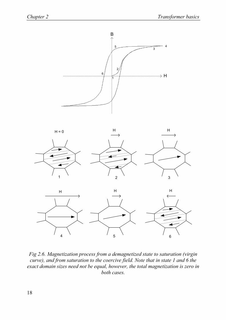
Fig 2.6 illustrates the magnetization processes for a soft magnetic material that is first brought from a demagnetized state up into saturation. Then, it is brought to a remanent state by removal of the field. Finally, it is brought back to a state where the resulting magnetization is zero. The final step is achieved by applying a reversed field. In that procedure the following magnetization processes [23], [29] are present:
1. In a demagnetized state the material consists of domains with different magnetization such that the total magnetization in the material is zero. When applying a low field the domain walls start to bulge like an elastic membrane, which is a reversible process.
2. At low to intermediate field strength, the domains with magnetization direction close to the applied field start to grow in size. Thereby, the domain walls move, which is an irreversible process.
Transformer basics Chapter 2
17
3. Increasing the field, eventually one large domain is created with magnetization direction along the crystallographic easy axis* closest to the applied field. This is also an irreversible process and now the material is technically saturated.
4. If the field is increased even further, the magnetic moments will slowly rotate into the field direction. This is a reversible process.
5. Now, if the field is decreased the moments will rotate back to the easy axis closest to the applied field direction.
6. If the applied field changes direction the material is split up into domains with different magnetization directions again. Now, a state where the total magnetization is zero is reached although the applied field is nonzero. This field is called the coercive field.
* E.g., in iron, the atoms are bonded together in a cubic crystal. In this case the moments of the atoms can align easily along the sides of the cube. Thereby, these directions are easily magnetized and therefore called easy axes. Conversely, the diagonal directions in the cube are hard to magnetized and therefore called hard axes [27].
Chapter 2 Transformer basics
18
H
B
H = 0
1
2
1 2
H
3
H
345
6
4
H H H
6
4 5 6
Fig 2.6. Magnetization process from a demagnetized state to saturation (virgin curve), and from saturation to the coercive field. Note that in state 1 and 6 the
exact domain sizes need not be equal, however, the total magnetization is zero in both cases.
Transformer basics Chapter 2
19
2.2.2 Dynamic properties of magnetic materials When the rate of change (e.g. the frequency) of the flux is increased, the hysteresis loop increases in width. This effect is due to rate-dependent magnetization processes and is usually divided into classical eddy currents and excess loss. These rate-dependent effects are sometimes referred to as dynamic hysteresis.
In this section infinite long sheets of magnetic materials are considered. Thereby, the magnetization is restricted to one dimension, i.e., along the axis perpendicular to the cross-sectional plane of the sheet. Therefore, the scalar expressions are used for B, H and M.
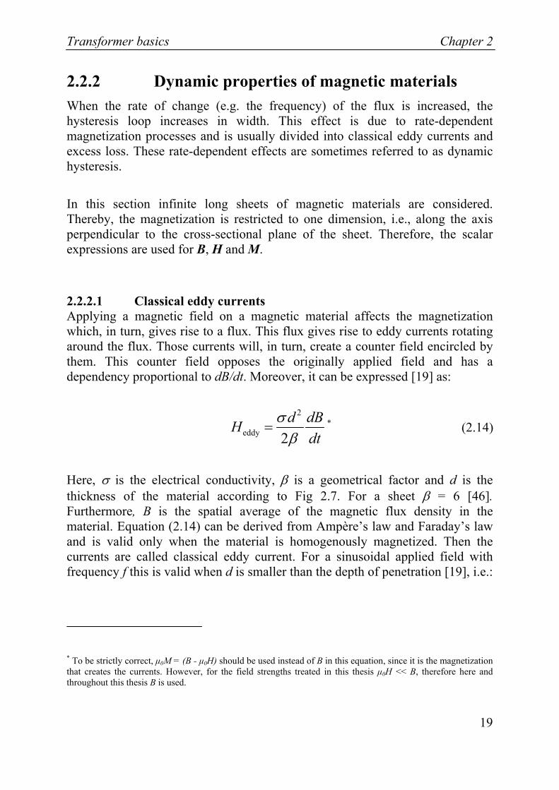
2.2.2.1 Classical eddy currents Applying a magnetic field on a magnetic material affects the magnetization which, in turn, gives rise to a flux. This flux gives rise to eddy currents rotating around the flux. Those currents will, in turn, create a counter field encircled by them. This counter field opposes the originally applied field and has a dependency proportional to dB/dt. Moreover, it can be expressed [19] as:
2
eddy 2d dBH
dtσβ
= * (2.14)
Here, σ is the electrical conductivity, β is a geometrical factor and d is the thickness of the material according to Fig 2.7. For a sheet β = 6 [46]. Furthermore, B is the spatial average of the magnetic flux density in the material. Equation (2.14) can be derived from Ampère’s law and Faraday’s law and is valid only when the material is homogenously magnetized. Then the currents are called classical eddy current. For a sinusoidal applied field with frequency f this is valid when d is smaller than the depth of penetration [19], i.e.:
* To be strictly correct, μ0M = (B - μ0H) should be used instead of B in this equation, since it is the magnetization that creates the currents. However, for the field strengths treated in this thesis μ0H << B, therefore here and throughout this thesis B is used.

Chapter 2 Transformer basics
20
r 0
1dfπμ μ σ
< (2.15)
If the condition in equation (2.15) is not satisfied, eddy current shielding will occur. This means that the inner regions of the material will exhibit greater opposing field caused by the eddy currents than the outer regions. Since Heddy increases with frequency, the shielding effect will also increase with frequency. Moreover, the field amplitude will increase with the distance from the midpoint of the material. Now the field distribution inside the material is inhomogeneous and the classical eddy current expression can not be used directly. In this thesis another model using a ladder network called Cauer circuit is presented. That model divides the cross-section of the material into smaller regions where the classical eddy current formulation is valid. This technique is presented in section 4.2.1.
dBdt
Fig 2.7. Eddy currents in a magnetic sheet.
2.2.2.2 Excess loss It is common to consider the difference between the total magnetic loss in a material and the contributions from static hysteresis and eddy current losses as excess or anomalous losses. The main part of the excess loss is considered to origin from the domain wall movements when magnetizing a material. These movements will introduce locally flux changes which, in turn, induce microscopic eddy currents [19]. This loss is rate-dependent.
A statistical loss theory built on a phenomenological description of the magnetization in which there are a number of active correlation regions

Transformer basics Chapter 2
21
randomly distributed in the material has been proposed by Bertotti [19], [30]. The correlation regions are connected to the microstructure of the material like grain size, crystallographic textures and residual stresses. Hereby the magnetic field created by the excess losses can be expressed as:
0 0excess 2
0 0
41 1 sign2
n V Gdw dB dBHn V dt dtσ ⎞⎛ ⎞⎛= + − ⎟⎜ ⎜ ⎟⎜ ⎟ ⎝ ⎠⎝ ⎠
* (2.16)
In equation (2.16), w is the width of the laminate according to Fig 2.7. Furthermore, G is a parameter depending on the structure of the magnetic domains. n0 is a phenomenological parameter related to the number of active correlation regions when f → 0, whereas V0 determines how much microstructural features affect the number of active correlation regions. The latter parameter also depends on the amplitude of the magnetization.
When
20 0
4 1Gdwn Vσ
>> (2.17)
equation (2.16) can be simplified to:
excess 04 signdB dBH GdwVdt dt
σ ⎞⎛= ⎜ ⎟⎝ ⎠
(2.18)
This is usually the case for electrical steels.
2.2.2.3 Total field The total magnetic field inside a material can be expressed as:
* See footnote to equation (2.14).

Chapter 2 Transformer basics
22
tot stat eddy excessH H H H= + + (2.19)
where Hstat represents the field corresponding to the static hysteresis. Using equations (2.14) and (2.18) in equation (2.19) yields:
2
tot stat 04 sign2d dB dB dBH H GdwV
dt dt dtσ σβ
⎞⎛= + + ⎜ ⎟⎝ ⎠
(2.20)
This results in a broadening of the B-H loop as seen in Fig 2.8. The static part gives rise to the rate-independent effect and Heddy and Hexcess give rise to the dynamic effects and thereby a broadening of the curve. From equation (2.20) we find that the relation between H and B is very complex, far from the linear approximation of the relative permeability that sometimes is used.
Fig 2.8. Composition of a dynamic magnetization curve at moderate frequencies for electrical steels. Solid line: Hstat. Dashed line: Hstat + Heddy. Dotted line: Htot = Hstat + Heddy + Hexcess. For higher frequencies the dashed and dotted lines can
be rounded.

Transformer basics Chapter 2
23
The total energy loss per volume of the magnetic material for one loop with period time T can be written as:
322 2
tot stat 00
42
T dB d dB dBW H GdwV dtdt dt dt
σ σβ
⎞⎛⎞⎛ ⎟⎜= + +⎜ ⎟ ⎟⎜ ⎝ ⎠
⎝ ⎠∫ (2.21)
where T is the period time for one loop.
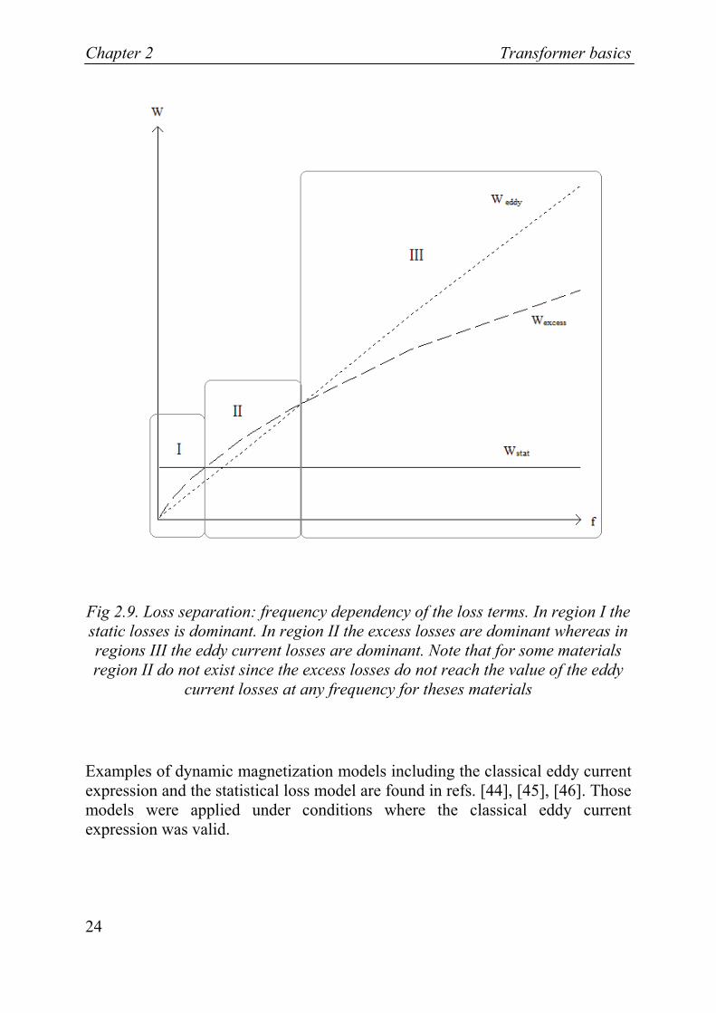
We can see from equation (2.21) that the static magnetization loss varies linearly with dB/dt, the classical eddy currents loss has a square dependency of dB/dt and the excess loss varies with (dB/dt)3/2. The parameter values will affect the absolute values of the terms; however, the following relation is usually valid: the static loss is dominant at low frequencies, whereas the excess loss is highest in the mid-frequency range and the classical eddy current loss i dominant for high frequencies. This is illustrated in Fig 2.9.
Chapter 2 Transformer basics
24
Fig 2.9. Loss separation: frequency dependency of the loss terms. In region I the static losses is dominant. In region II the excess losses are dominant whereas in regions III the eddy current losses are dominant. Note that for some materials region II do not exist since the excess losses do not reach the value of the eddy
current losses at any frequency for theses materials
Examples of dynamic magnetization models including the classical eddy current expression and the statistical loss model are found in refs. [44], [45], [46]. Those models were applied under conditions where the classical eddy current expression was valid.

Transformer basics Chapter 2
25
2.2.2.4 Another description of dynamic magnetization There are also other dynamic magnetization models available in literature. One recent model that has attracted some attention is the viscosity-based magnetodynamic model suggested by Zirka et al. [33], [34], [35], [36]. In that model the dynamic effects are considered as a lag of B behind H, i.e., magnetic viscosity. A semi empirical model has been developed which consist of one static and one dynamic term:
( ) ( )1
tot stat signdBH H g B Bdt
α= + (2.22)
In the first approach, α is a material constant close to 2 for electrical steels and g(B) is defined as:
( ) m2
2S
1
Gg BBB
=⎛ ⎞⎟⎜ ⎟−⎜ ⎟⎜ ⎟⎜⎝ ⎠
(2.23)
Here Bs is the saturation flux density and Gm is a material constant.
In ref. [34] it was showed that this model yields satisfying results up to 500 Hz for one grain oriented material. It was, however, later shown that in order to simulate other non oriented and grain oriented materials, the definitions of g(B) and α needed to be updated [33], [35]. These were changed such that, e.g., α had a dependency of B and the simple relation in equation (2.23) was changed to a 4:th and even 6:th degree polynomial of B. Furthermore, α:s and g(B):s dependency of B differed for different values of B. It is obvious that this method requires much adapting of the parameters to fit the B-H curves. Nevertheless, this method was as best able to replicate the measured curves up to around 1 kHz. However, the high number of adapting steps for each material makes the usability of this model questionable.
2.2.3 Additional loss sources in real cores Until now the core has been considered to consist of one magnetic sheet. In reality, however, the core consists of a laminate of stacked sheets. Usually the
Chapter 2 Transformer basics
26
sheets are clamped together which can induce stresses in the material and lead to magnetostrictive losses [1]. Another source of increased losses can be “burrs” on the core laminations edges, i.e., rough areas which can create locally high eddy current losses [26]. Furthermore, aging of the material can also decrease the permeability and increase the magnetic losses in the core [78], [79], [80].
Another source of losses origins from the joints between the legs and yokes of the transformer. One reason to this is small air gaps in the joint. Another reason is that oriented materials, which have high anisotropy, are used. In the joints the flux direction is changed by 90°, however, by constructing a 45° mitred joint the losses are decreased. Nevertheless, they have to be considered in the calculation of the total losses of the core [1], [26].
2.3 Losses in the winding
2.3.1 Losses in the winding conductors The electromagnetic losses in the winding conductors consist of three major parts:
• Resistive or ohmic losses
• Skin effect losses
• Proximity effect losses
There has been some confusion about the term eddy currents in the literature. Some authors intend the proximity effect only and some others intend both the proximity effect and the skin effect [13], [20]. The latter meaning is used in this thesis.
The skin effect appears in a conductor during AC conditions when the current creates an alternating magnetic flux circulating around the current. This flux, in turn, creates an opposing current inside the conductor. With increasing frequency the opposing current will increase in amplitude and the current will

Transformer basics Chapter 2
27
flow in a thin shell in the outer part of the conductor. This is in analogy with the magnetic eddy current effect.
Furthermore, when a number of conductors are placed close together, the H-field created by the current in one conductor will create eddy current losses in the nearby conductors. This is called proximity effect and occurs in the transformer windings where the conductors are exposed to H-fields created by the other conductors.
2.3.2 Other loss mechanisms in the windings There are two other major loss mechanisms that are present in the winding window:
• Dielectric loses due to capacitive effects. The capacitive effects consist of, e.g., capacitances between individual turns, between discs or layers in a winding, between windings and between core and windings. The capacitances give rise to uneven voltage distribution in the windings, especially during transient conditions. At high frequencies, typically higher than 100 kHz, also dielectric losses in the insulating materials between conductors and discs or layers, become apparent [58], [69].
• Leakage flux. Since the magnetic core has finite permeability all of the magnetic flux created by the currents in the conductors will not be confined inside the core. Conversely, it will be present also in the winding window. In a no-load condition this is not a big issue, since only the magnetizing current is existent and this current is so small that the flux created in the winding window is negligible [26]. However, in a load condition the winding currents are much higher and therefore the flux through the conductors is significant. This flux can cause considerably eddy current losses in the winding conductors. Furthermore, the fraction of this flux that induces a voltage in only one of the windings and not in both gives rise to a reactive power loss. That part is here defined as leakage flux [1]. This flux is resident between the windings and inside the outer winding and corresponds to the short-circuit reactance of the transformer.


Winding model Chapter 3
29
Chapter 3
Winding model
The winding types can be divided into four categories with regard to their mechanical design [1], [20]:
• Layer winding. The conductor is wound with succeeding turns along the axial direction of the core, constituting one layer. Thereby, the turns in one layer are connected in series. Multilayer windings consist of multiple numbers of layers connected in series with each other.
• Helical winding. This type consist of parallel wound conductors. The conductors are usually wound as a layer winding, however, with spacer between the turns.
• Foil winding. Consists of sheets of conducting materials with a width equal to the winding height and wound in a spiral around the core.
• Disc winding. Has two common winding techniques:
– Conventional. The conductor is wound with succeeding turns outside each other in a spiral. When the space for one disc is filled up the conductor continues with turns below or above the first disc.
– Interleaved. For a pair of discs, first half of the turns are wound in the first disc and then half of the turns in the next disc. Then the remaining turns are wound in the first disc and finally the last turns in the second disc. This procedure is continued for all pair of discs
Chapter 3 Winding model
30
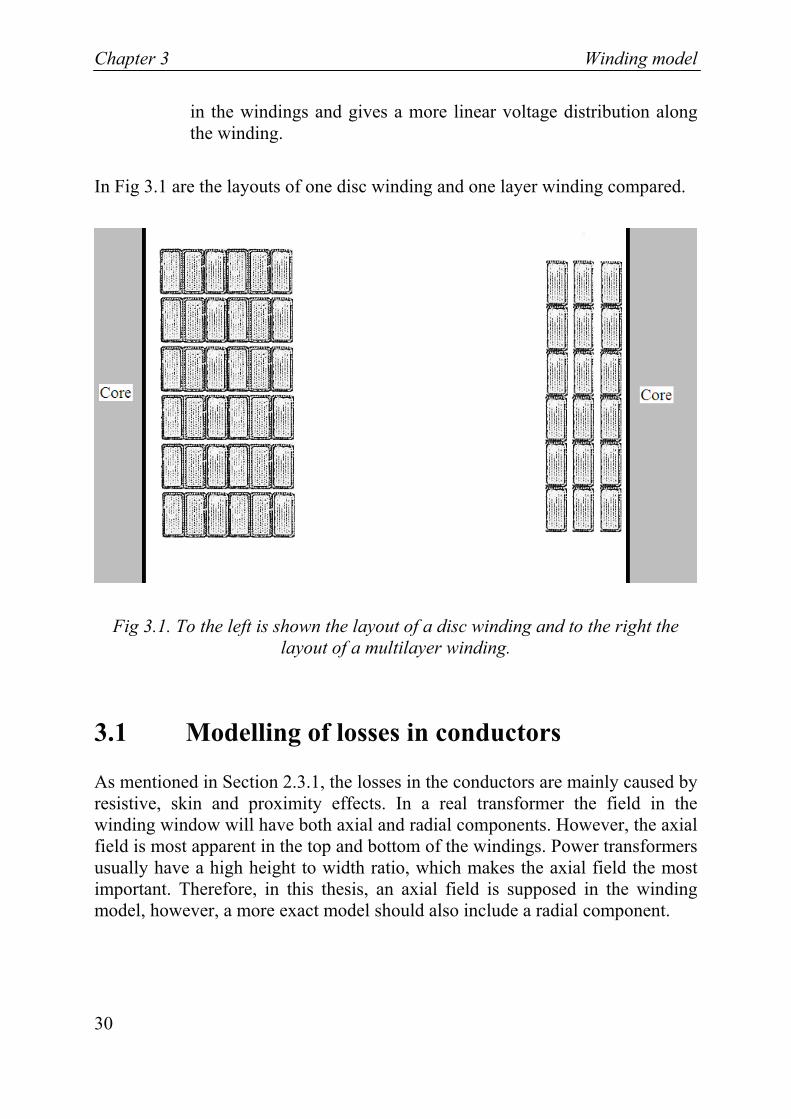
in the windings and gives a more linear voltage distribution along the winding.
In Fig 3.1 are the layouts of one disc winding and one layer winding compared.
Fig 3.1. To the left is shown the layout of a disc winding and to the right the layout of a multilayer winding.
3.1 Modelling of losses in conductors
As mentioned in Section 2.3.1, the losses in the conductors are mainly caused by resistive, skin and proximity effects. In a real transformer the field in the winding window will have both axial and radial components. However, the axial field is most apparent in the top and bottom of the windings. Power transformers usually have a high height to width ratio, which makes the axial field the most important. Therefore, in this thesis, an axial field is supposed in the winding model, however, a more exact model should also include a radial component.

Winding model Chapter 3
31
3.1.1 Analytical expression for eddy currents There exists, in literature, different analytical expressions for the eddy currents in coil conductors. Among these are the approaches of Dowell [65], Ferreira [66] and Perry [20], [21], [22]. Moreover, comparisons of these expressions are found in refs. [67], [68] and [72]. In ref. [68] two experimental comparisons are made on 1) a two layer air-core inductor and 2) a three layer iron core inductor. In these comparisons it is shown that Perry’s and Dowell’s expressions are in better agreement with measurements than Ferreira’s expression. It is also shown that for the iron core coil Perry’s expression is more correct than Dowell’s. Therefore, in this thesis Perry’s method is used.
Perry derives an analytical expression for the electromagnetic losses in a coil including resistive, skin effect and proximity effect losses [20], [21], [22]. Looking at the coil as a network of resistive and inductive elements excited through a single external terminal pair and comprising all electromagnetic properties in the coil, an equivalent impedance is derived, see Fig 3.2. The excitation source is assumed to be sinusoidal at a fixed angular frequency ω. Since the material in the coil has a constant permeability the electromagnetic response in the network will also be sinusoidal with angular frequency ω.
Here follows a short description of the procedure for calculation of the expression. For a more detailed derivation of the expression see Appendix I.
Fig 3.2. Network of resistive and inductive elements excited by an external source through a terminal pair.
Starting with Maxwell’s equations and using the Poynting theorem, it is possible to express the input power through the terminals as a function of the current

Chapter 3 Winding model
32
density, J, and magnetic field H. Moreover, one can derive an equivalent impedance of the coil expressed as a function of J and H in complex notation as:
*2 2
1 ˆ ˆ ˆ ˆ( j ) jˆ ˆ2 2V V
Z dV dVI I
ωμωσ
∗= −∫ ∫J J H Hi i (3.1)
where I is the current going through the terminal, J is the current density and H the magnetic field inside the coil. Moreover “^” denotes a complex amplitude.
Now, by finding J and H inside the coil it is possible to determine the impedance with use of equation (3.1). Consider the coil geometry as seen in Fig 3.3 with every turn having equal width and height. Solving the magnetic diffusion equation in rectangular coordinates (which is valid when the diameter of the coil is much larger than the thickness of one conductor), one gets the following expressions for H and J in the n:th turn:
( ) ( )( ) ( ) ( )( )( )( )
1,
1
ˆ sinh 1 sinhˆsinh
n nn z
n n
n k y y n k y yIH yw k y y
−
−
⎡ ⎤− − − −= ⎢ ⎥
−⎢ ⎥⎣ ⎦ (3.2)
( ) ( )( ) ( ) ( )( )( )( )
1,
1
ˆ cosh 1 coshˆsinh
n nn x
n n
n k y y n k y ykIJ yw k y y
−
−
⎡ ⎤− − − −= ⎢ ⎥
−⎢ ⎥⎣ ⎦ (3.3)
where k is the complex wave number and n is the layer number counted inwards when Hz is increasing inwards and counted outwards when Hz is increasing outwards. E.g. for a single coil, n is counted inwards. Moreover, k is defined as:
( j 1)kδ+
= (3.4)

Winding model Chapter 3
33
where δ is the skin depth or depth of penetration defined as*:
2δ
ωμσ= (3.5)
Fig 3.3. Cross-section of a portion of a multilayer coil with an arbitrary number of turns. The current is directed along the negative x-axis.
* Compare with equation (2.15).

Chapter 3 Winding model
34
Furthermore, the whole part of the field in the coil is assumed to be generated in the coil itself, i.e., no field is penetrating the coil from outer sources. The field distribution when the field is increasing inwards is then as seen in Fig 3.4. Moreover, the field is assumed to only have an axial component and no radial component. This is an approximation; however, if the axial dimension is much larger than the radial, then the axial field is much larger than the radial field and the approximation is valid.
I
N
Symmetry axis
H, φ
Fig 3.4. Cross-sectional view of one side of a coil showing the field distribution in axial direction.
Using equations (3.2) and (3.3) in equation (3.1) and integrating over one turn in layer n with the circumference ln and height w yields:
( ) ( ) ( ) ( )1 1
2 2ˆ ˆ ˆ ˆj
ˆ ˆ2 2
n n
n n
y yn n
n x x z zy y
l w l wZ J y J y dy H y H y dyI I
ωμ
σ − −
∗ ∗= −∫ ∫ (3.6)

Winding model Chapter 3
35
Setting in equations (3.2) and (3.3) in equation (3.6) and performing the calculations yields:
( )
( )
21 2
23 4
2 2 1 ( ') 4 ( 1) ( ')2
j 2 2 1 ( ') 4 ( 1) ( ')4
nn n n
nn n
lZ n n F d n n F dw
l n n F d n n F dw
σδωμδ
⎡ ⎤= − + − − +⎣ ⎦
⎡ ⎤+ − + − −⎣ ⎦
(3.7)
where
nn
ddδ
′ = (3.8)
and F1, F2, F3 and F4 are functions given as:
1sinh(2 ') sin(2 ')( ')cosh(2 ') cos(2 ')
n nn
n n
d dF dd d
+=
− (3.9)
2sinh( ')cos( ') cosh( ')sin( ')( ')
cosh(2 ') cos(2 ')n n n n
nn n
d d d dF dd d
+=
− (3.10)
3sinh(2 ') sin(2 ')( ')cosh(2 ') cos(2 ')
n nn
n n
d dF dd d
−=
− (3.11)
4sinh( ')cos( ') cosh( ')sin( ')( ')
cosh(2 ') cos(2 ')n n n n
nn n
d d d dF dd d
−=
− (3.12)
Now we have managed to find an analytical expression for the impedance of every single turn in a coil carrying a sinusoidal current. Identification of the terms in equation (3.7) shows that the first term on the right side corresponds to the resistive effect and the second term to the reactive.

Chapter 3 Winding model
36
In the transformer application with two windings (or coils) the layer number n is counted inward for the outer winding and outward for the inner winding. In this case the axial component of the field is as shown in Fig 3.5.
I2
N2
I1
N1
Core
Symmetry axis
H, φ
Fig 3.5. Axial field distribution in a winding window of a two-winding transformer.
3.1.1.1 Equivalent circuits In order to use these expressions in a circuit simulation program, like Dymola*, an equivalent circuit has to be created. In this case it is easily done, since equation (3.7) consists of one resistive and one inductive part. Therefore, a resistance, R, is connected in series with an inductance, L, in order to simulate the equivalent impedance in every turn. The total impedance in one turn is given by:
jn n nZ R Lω= + (3.13)
* Dymola – Dynamic Modeling Laboratory, Dynasim AB, Sweden. www.dynasim.se

Winding model Chapter 3
37
where
( )21 22 2 1 ( ') 4 ( 1) ( ')
2n
n n nlR n n F d n n F d
wσδ⎡ ⎤= − + − −⎣ ⎦ (3.14)
and
( )23 42 2 1 ( ') 4 ( 1) ( ')
4n
n n nlL n n F d n n F d
wμδ ⎡ ⎤= − + − −⎣ ⎦ (3.15)
3.1.1.2 Discussion In the derivation of the eddy current expression it is assumed that the radial flux is negligible compared to the axial flux. It is also supposed that there are no capacitive effects between the turns. This is an approximation which is valid in a certain frequency range. It has been shown that the upper frequency limit is around 100 kHz for an inductor with iron core [68]. Moreover, one can understand that for higher frequencies both the radial flux and capacitive effects will affect the field distribution. Therefore, at higher frequencies, the linear increasing field distribution as shown in Fig 3.5 will not be valid and neither will equation (3.7) be.
3.2 Modelling of capacitive effects
The importance of the capacitive effects in transformer models is dependent on which frequency range it should be used for. E.g., at frequencies up to around 1 kHz the capacitances are negligible [1]. Above that the capacitances between winding and core/tank and between discs become important [1]. For frequencies above approximately 100 kHz also the capacitances between individual turns are essential [69].
A proposed disc winding model including capacitances between discs and discs and core/tank is shown in Fig 3.6. In this model the inter-turn capacitances are omitted. Moreover, the capacitances between turns in two adjacent discs are lumped to one capacitance.
Chapter 3 Winding model
38
• The impedance for each turn is calculated using equation (3.13). The turns in a disc are connected in series and we do not consider the capacitances between them. Therefore, the turn impedances in a disc can be connected together in series to constitute the total impedance for one disc. The total impedance of a disc is represented by the series connected Rd and Ld in the figure. This gives a resulting impedance for a disc with M turns as:
d d d1 1
j jM M
n nZ R L R Lω ω= + = +∑ ∑ (3.16)
• The disc to disc capacitance is shunted with the impedance in the disc and denoted Cd in the figure. Notice that for the discs in the ends of the windings the capacitance must be Cd/2. This gives the correct value of the total series disc capacitance of the winding.
• The capacitances between every disc in a winding to the closest disc in the other winding are named Cwind-wind. Furthermore, the capacitances between the windings and core, yoke and tank wall, respectively, are denoted Cwind-core, Cwind-yoke and Cwind-wall, respectively. The core, yoke and wall are grounded.

Winding model Chapter 3
39
Rd
LdCd/2
Rd
LdCd
Rd
LdCd/2
Rd
LdCd/2
Rd
LdCd
Rd
LdCd/2
Cwind-yoke
Cwind-core
Cwind-yokeCwind-wall
Cwind-wall
Cwind-yoke
Cwind-wind
Cwind-wind
Disc 1 Disc 1
Disc 2 Disc 2
Disc N1Disc N2
Cwind-wind
Cwind-wind
Cwind-wind
Cwind-wall
Cwind-wall
Cwind-core
Cwind-core
Cwind-core
Cwind-yoke
Connection to net, wind 1
Connection to net, wind 1
Connection to net, wind 2
Connection to net, wind 2
Fig 3.6. Electrical network showing the impedances in the discs and the capacitances between discs and between discs and surrounding material. The
impedances comprise the equivalent circuit for the ohmic and eddy current losses in the conductors as presented in the previous section.

Chapter 3 Winding model
40
3.2.1 Discussion The model has a theoretical upper frequency limit around 100 kHz due to the earlier mentioned restrictions of the eddy current expression and the resolution of the capacitances. However, this should be verified through measurements.
Here, an electrical network for a disc winding has been used as example. It is, however, possible to derive the corresponding networks for the other type of windings.
3.3 Modelling of flux in the winding
In order to calculate the flux in the winding window let us consider the axial field distribution as shown in Fig 3.7.
Fig 3.7. Axial field distribution in a winding window also indicating the different flux regions.

Winding model Chapter 3
41
According to Fig 3.7 it is possible to divide the core and winding area into five different regions:
Region 1: core
Region 2: between core and inner winding
Region 3: inner winding
Region 4: between the windings
Region 5: outer winding
Now, the flux in each region can be calculated using, the following expression, which origins from Ampère’s law (equation (2.1)):
i ii
i
A Il
μϕ = , (3.17)
where Ii is the sum of the current encircling the region i, whereas li is the averaged magnetic path length of the flux and Ai is the cross-section area which the flux flows through in region i.
Now, let us consider the sum of the encircling currents for the different regions, which will be as follows:
• Region 1 and 2: N1I1 + N2I2, where N1 and N2 are the number of turns in the inner and outer winding, respectively and I1 and I2 are the currents in the corresponding winding.
• Region 3: N1I1/2 + N2I2. From the ampère-turn diagram one can understand that the flux in a given turn in the inner winding will be proportional to the current in the outer winding plus the currents in all other turns with a larger radius than that turn in the inner winding. The average flux in the inner winding caused by the currents in the same

Chapter 3 Winding model
42
winding will then be proportional to N1I1/2 since the flux increases approximately linearly.
• Region 4: N2I2.
• Region 5: N2I2/2. Same argument as for region 3.
Now, from Faraday’s law, equation (2.2), the induced voltage in the windings is given as:
inddUdtϕ
=− (3.18)
where φ is the sum of all flux that is encircled by each winding, respectively. E.g., for the outer winding, combining equations (3.17) and (3.18), yields:
5
core1
ind,outer
5
core1
ii
ii
i i
ddUdt dt
Ad Il
dt
ϕ ϕϕ
ϕ μ
=
=
⎛ ⎞⎟⎜ + ⎟⎜ ⎟⎟⎜⎝ ⎠=− =− =
⎛ ⎞⎟⎜ + ⎟⎜ ⎟⎜ ⎟⎝ ⎠=−
∑
∑ (3.19)
where i = 1, 2, 3, 4, 5 corresponds to the each regions, respectively. Ii is calculated as previously shown and φcore is given from a core model.
3.3.1 Discussion The model for the flux in the winding is supposed to be valid in the same frequency region as the eddy current expression, i.e. up to around 100 kHz. This is since they both build on the field distribution as illustrated in Fig 3.7. This distribution does only include the axial direction of the field, however, for higher frequencies the radial direction has to be included.

Core model Chapter 4
43
Chapter 4
Core model
4.1 Static magnetization model
There exists a wide variety of static hysteresis models in literature today. The most common are the Jiles-Atherton model [29], [37], [38] and the Preisach model [39], [40], [41]. However, in this work the model originally proposed by Bergqvist [23], [24], [25] is used. This model has some similarities with the above mentioned models. E.g., the pinning of domain wall motion introduced in the Jiles-Atherton model is used. Moreover, the use of sets of simpler elements to build up a complex hysteretic relation is taken from the Preisach model. It also has similarities to mechanical hysteresis models. Benefits with the Bergqvist model is that it is easy to use and can be understood intuitively. Furthermore, it is intrinsic multidimensional and allows direct handling of magnetomechanical hysteresis.
In the next section a short survey of the model is presented, however more details are found in refs. [23], [24], [25] , [42] and [43].
4.1.1 Bergqvist’s lag model At a given time, a magnetic material consists of magnetic domains with different magnetization amplitude and direction. In Bergqvist’s lag model all domains with equal magnetization are lumped into volume fractions of the whole material. These volume fractions are called pseudo particles. Moreover, the total

Chapter 4 Core model
44
magnetization in the material is a weighted sum of the individual magnetization of all pseudo particles.
4.1.1.1 One dimensional model With no hysteresis present, the magnetization would follow an anhysteretic curve. The hysteresis is introduced by a play operator operating on the anhysteretic curve. Moreover, the pinning strength, or size, k, of the play operator, will determine the width of the hysteresis curve. This operation is shown in Fig 4.1 where m is the magnetization of a pseudo particle and H is the applied field on that pseudo particle. Moreover, η is the magnetizing field, which in absence of pinning would produce the anhysteretic magnetization. Mathematically η, which also is called back field, can be written [42] as:
( ) if ( ) ( )( ) ( ) if ( ) ( )
( ) if ( ) ( )
t t H t t t kt H t k H t t t k
H t k H t t t k
η ηη η
η
Δ Δ
ΔΔ
⎧ − − − ≤⎪⎪⎪⎪= − − − >⎨⎪⎪ + − − <−⎪⎪⎩
(4.1)
The linear play operator, as depicted in Fig 4.1 is defined as:
[ ]kP H η= (4.2)
For a field change of ΔH the play operator yields:
[ ][ ] [ ]
[ ][ ]
k k
k k
k
if
if
if
P H H H P H k
P H H H H k H H P H k
H H k H H P H k
Δ
Δ Δ Δ
Δ Δ
⎧⎪ + − <⎪⎪⎪+ = + − + − ≥⎨⎪⎪⎪ + + + − ≤−⎪⎩
(4.3)

Core model Chapter 4
45
Fig 4.1. To the left an anhysteretic curve is seen. In the middle is a play function which operates on the anhysteretic curve and generates the hysteresis curve
seen to the right.
4.1.1.2 Multi dimensional model In n dimensions −H η will be the driving quantity. Using the notation
( )( ) ( )t t tΔ= − −w H η the play-operator can be written:
( )
1
11 1
if 1( ) ( )
1 if 1t t tΔ
−
−− −
⎧⎪ ≤⎪⎪⎪− − =⎨⎪ − >⎪⎪⎪⎩
0 k wη η
k w w k w (4.4)
Here, k is a symmetric tensor that represents the pinning strength in n dimensions [23].
By using a finite number of pseudo particles, minor loops can be modelled as well. This is achieved by assigning an individual pinning strength, λik, to every pseudo particle, where k is the mean pinning strength of all pseudo particles and λi is a dimensionless multiplier for pseudo particle i. Thereby, the total magnetization is given by a weighted superposition of the contributions from all pseudo particles, see Fig 4.2.

Chapter 4 Core model
46
Fig 4.2. Weighted superposition of the contributions from the minor loops.
The total multi dimensional magnetization can be expressed:
[ ]( )an an λ0
( ) ( )c M P dς λ λ∞
= +∫ kM M H H (4.5)
The first term on the right side of equation (4.5) represents the reversible part of the magnetization, referring to section 2.2.1.4. Here, Man comprises the anhysteretic magnetization, which would be the magnetization if no hysteresis was present. The parameter c governs the degree of reversibility of the magnetization and defined as:
0
an
(0)(0)
c χχ
= (4.6)
where χ0 (0) corresponds to the linear portion of the susceptibility of a virgin curve and χan (0) is the susceptibility of the anhysteretic curve at H = 0. This implies that c is set to a constant; however, this would not necessarily be true for a real material. This is discussed more in detail in section 4.1.2.5.
The second term of the right side in equation (4.5) constitutes the hysteretic behaviour (irreversible part). This part does also follow the anhysteretic path, however, with a hysteresis effect introduced by the play operator Pλk. The play operator has the pinning strength λik for pseudo-particle i. Moreover, ς(λ) is the density function which gives the weight of the pseudo particles and can e.g. be a Gaussian distribution:
2( )( ) e p qA λς λ − −= (4.7)

Core model Chapter 4
47
This expression contains three unknown parameters A, p and q, governing the distribution. The following normalization conditions give two of the parameters:
0
( ) 1d cς λ λ∞
= −∫ (4.8)
0
( ) 1dλς λ λ∞
=∫ (4.9)
The third parameter could be found by linearizing Man for small H. This would yield the second order term of the virgin curve [42], [43] as:
2
0 01(0) (0) (0) e (0)
2 2qA
k kκ ς χ χ−= = (4.10)
The pinning strength, k, is given by the coercive field and by solving this equation system all parameters will be known. A complete walk-through of the parameter estimation procedure is found in Appendix II.
In the remaining parts of the thesis the one dimensional case will be treated.
4.1.2 Modifications
4.1.2.1 Anhysteretic curve obtained from measurements In order to generate a correct hysteresis model it is of importance that the anhysteretic curve is modelled correctly. The most correct approach is to find it through measurements on a material. This can be done by slowly demagnetizing the material from saturation using an AC-field with different superimposed DC-fields [19], [29]. This yields a set of (B, H) - and (M, H) - values that correspond to the anhysteretic curve. The material should be far into saturation when starting the demagnetization and the major loop should be traversed a number of times before minor loops are cycled.
The DC-fields should be applied as slowly increasing fields, thereby decreasing the risk of unwanted rate-dependent effects which could be the effects if the

Chapter 4 Core model
48
fields were applied as step functions. Introducing a DC-field as a step in the start of the demagnetization process would also displace the demagnetization curve so that it may not reach negative saturation during the process.
Furthermore, the DC-fields should reach their final value before starting to traverse minor loops and keep those values until the applied AC-field diminishes. This is very important, since if the DC-fields are applied when the material does not reach saturation anymore, the reversal points of the demagnetization minor loops would be too low. This is due to the fact that the AC-field is continuously decreasing and even if the correct DC-fields are applied the magnetization would then not reach the correct values at the reversal points due to the hysteresis.
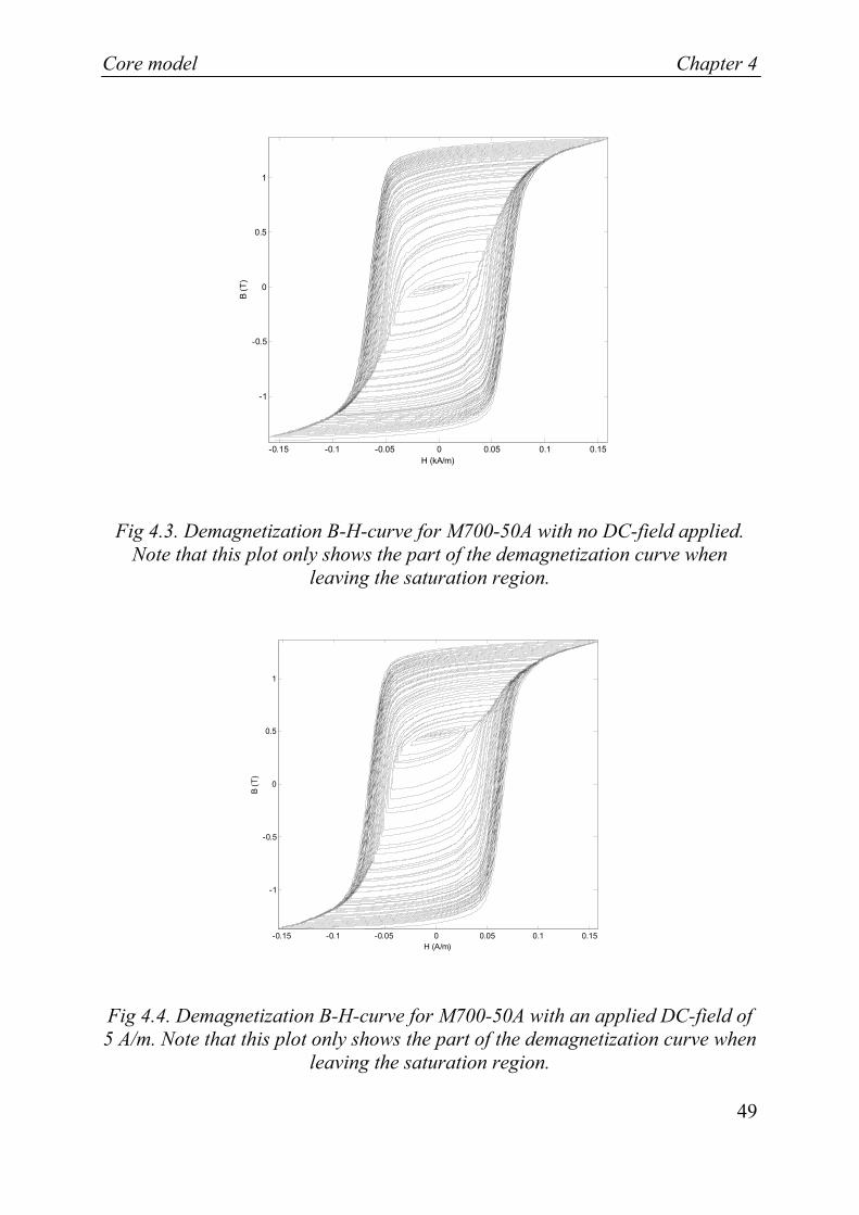
In Fig 4.3. - Fig 4.6 is shown an example of demagnetization of a sample of the non oriented electrical steel M700-50A*. Fig 4.3. and Fig 4.4 show demagnetization curves without and with a superimposed DC-field, respectively. Fig 4.5 shows the applied AC-field with a superimposed DC-field whereas Fig 4.6 shows the resulting B-field. The AC-field consists of an exponentially decreasing sinusoidal H-field at 0.04 Hz, which is considered as sufficiently slow not to introduce rate-dependent processes. However, the fast decrease at low amplitudes of B may introduce errors. A better method would be to control the B-field instead.
The anhysteretic curve for M700-50A found with different applied DC-fields is shown in Fig 4.7.
* For the measurement and simulation results shown in this chapter, the rolling direction of M700-50A is considered.
Core model Chapter 4
49
-0.15 -0.1 -0.05 0 0.05 0.1 0.15
-1
-0.5
0
0.5
1
H (kA/m)
B (T
)
Fig 4.3. Demagnetization B-H-curve for M700-50A with no DC-field applied. Note that this plot only shows the part of the demagnetization curve when
leaving the saturation region.
-0.15 -0.1 -0.05 0 0.05 0.1 0.15
-1
-0.5
0
0.5
1
H (A/m)
B (T
)
Fig 4.4. Demagnetization B-H-curve for M700-50A with an applied DC-field of 5 A/m. Note that this plot only shows the part of the demagnetization curve when
leaving the saturation region.

Chapter 4 Core model
50
0 500 1000 1500 2000 2500-20
-15
-10
-5
0
5
10
15
20
25
t (s)
H (k
A/m
)
Fig 4.5. Applied AC-field with applied DC-field of 5 A/m giving rise to the demagnetization curve in Fig 4.4.
0 500 1000 1500 2000 2500-2
-1.5
-1
-0.5
0
0.5
1
1.5
2
B (T
)
t (s)
Fig 4.6. B-curve as result of the applied H-field shown in Fig 4.5.

Core model Chapter 4
51
0 0.2 0.4 0.6 0.8 1 1.2 1.4 1.6 1.8 2
0
0.2
0.4
0.6
0.8
1
1.2
1.4
1.6
H (kA/m)
B (T
)
Fig 4.7. Major loop (solid lines) and anhysteretic curve (dashed line) for M700-50A. Rings indicate measured points. Notice that the major loop closes at higher
amplitude than shown in this plot.
The (M, H)-values of the anhysteretic curve could be used directly in the static magnetization model as comprising the anhysteretic magnetization.
4.1.2.2 Anhysteretic curve as mathematical function The drawback with achieving the anhysteretic curve from measurement is the amount of time it requires. Therefore, it is common to use mathematical functions that yield curve shapes that are similar to the real anhysteretic curve. Examples of adequate functions are tanh(), arctan() [25], Langevin [56] and Sigmoid [42].
The anhysteretic curve based on the arctan() function can be expressed as:
anan s 7
s
2 (0)( ) arctan8 10HM H MMχ
π −
⎞⎛= ⎟⎜ ⋅⎝ ⎠
(4.11)
Chapter 4 Core model
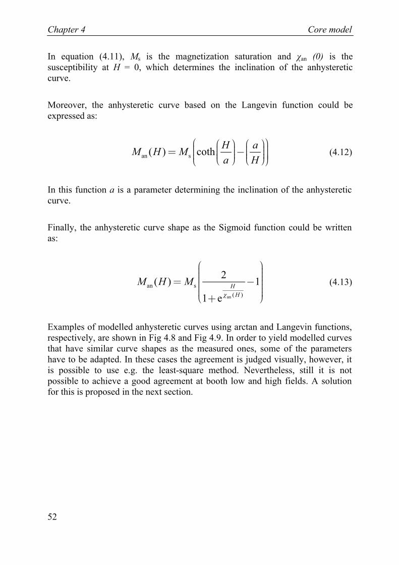
52
In equation (4.11), Ms is the magnetization saturation and χan (0) is the susceptibility at H = 0, which determines the inclination of the anhysteretic curve.
Moreover, the anhysteretic curve based on the Langevin function could be expressed as:
an s( ) coth H aM H Ma H
⎛ ⎞⎛ ⎞ ⎛ ⎞⎟⎟ ⎟⎜ ⎜ ⎜= − ⎟⎟ ⎟⎜ ⎜ ⎜ ⎟⎟ ⎟⎜ ⎜ ⎟⎜ ⎝ ⎠ ⎝ ⎠⎝ ⎠ (4.12)
In this function a is a parameter determining the inclination of the anhysteretic curve.
Finally, the anhysteretic curve shape as the Sigmoid function could be written as:
an
an s( )
2( ) 11 e
HH
M H Mχ
⎛ ⎞⎟⎜ ⎟⎜ ⎟⎜= − ⎟⎜ ⎟⎜ ⎟⎜ ⎟⎝ ⎠+
(4.13)
Examples of modelled anhysteretic curves using arctan and Langevin functions, respectively, are shown in Fig 4.8 and Fig 4.9. In order to yield modelled curves that have similar curve shapes as the measured ones, some of the parameters have to be adapted. In these cases the agreement is judged visually, however, it is possible to use e.g. the least-square method. Nevertheless, still it is not possible to achieve a good agreement at booth low and high fields. A solution for this is proposed in the next section.

Core model Chapter 4
53
Fig 4.8. Anhysteretic curves for M700-50A given from the arctan function with values of χan (0) and Ms adapted to yield good agreement of the slopes at low field and high field respectively. The measured anhysteretic curve (solid with
rings) is given as comparison.
Fig 4.9. Anhysteretic curves for M700-50A given from the Langevin function with values of a and Ms adapted to yield good agreement of the slopes at low field and high field respectively. The measured anhysteretic curve (dotted with
rings) is given as comparison.
Chapter 4 Core model
54
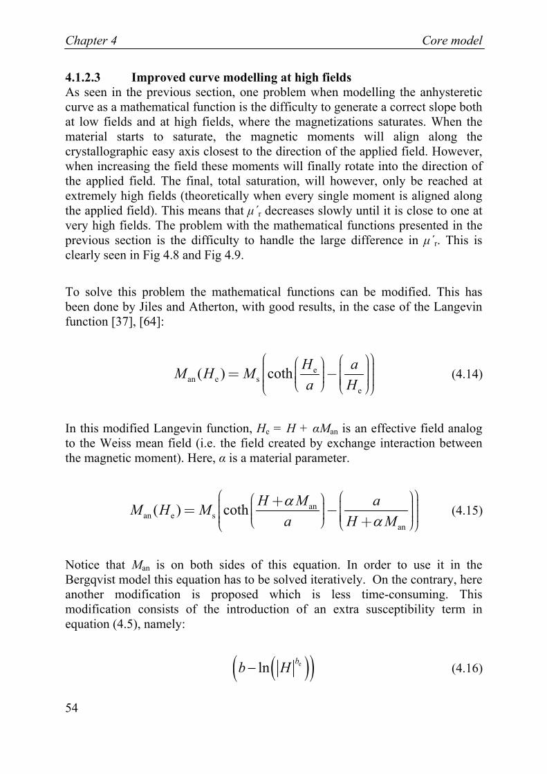
4.1.2.3 Improved curve modelling at high fields As seen in the previous section, one problem when modelling the anhysteretic curve as a mathematical function is the difficulty to generate a correct slope both at low fields and at high fields, where the magnetizations saturates. When the material starts to saturate, the magnetic moments will align along the crystallographic easy axis closest to the direction of the applied field. However, when increasing the field these moments will finally rotate into the direction of the applied field. The final, total saturation, will however, only be reached at extremely high fields (theoretically when every single moment is aligned along the applied field). This means that μ´r decreases slowly until it is close to one at very high fields. The problem with the mathematical functions presented in the previous section is the difficulty to handle the large difference in μ´r. This is clearly seen in Fig 4.8 and Fig 4.9.
To solve this problem the mathematical functions can be modified. This has been done by Jiles and Atherton, with good results, in the case of the Langevin function [37], [64]:
ean e s
e
( ) coth H aM H Ma H
⎛ ⎞⎛ ⎞⎛ ⎞ ⎟⎟⎜ ⎜⎟⎜ ⎟⎟= −⎜ ⎜⎟⎜ ⎟⎟⎜ ⎟⎜ ⎜ ⎟⎜ ⎟⎝ ⎠⎜ ⎝ ⎠⎝ ⎠ (4.14)
In this modified Langevin function, He = H + αMan is an effective field analog to the Weiss mean field (i.e. the field created by exchange interaction between the magnetic moment). Here, α is a material parameter.
anan e s
an
( ) coth H M aM H Ma H Mα
α
⎛ ⎞⎛ ⎞⎛ ⎞+ ⎟⎟⎜ ⎜⎟⎜ ⎟⎟= −⎜ ⎜⎟⎜ ⎟⎟⎜ ⎟⎜ ⎜ ⎟⎜ ⎟⎝ ⎠⎜ +⎝ ⎠⎝ ⎠ (4.15)
Notice that Man is on both sides of this equation. In order to use it in the Bergqvist model this equation has to be solved iteratively. On the contrary, here another modification is proposed which is less time-consuming. This modification consists of the introduction of an extra susceptibility term in equation (4.5), namely:
( )( )eln bb H− (4.16)

Core model Chapter 4
55
Here, b is a dimensionless constant and be a constant with unit (ln (A/m))-1. The values of b and be can be fitted for different materials from a measured major loop. Notice, that for H = 0, the logarithm is omitted. This yields the total magnetization:
( )( ) [ ]( )e
an an λk0
ln ( ) ( )bM b H H cM H M P H dζ λ λ∞
= − + +∫ (4.17)
The results using this logarithmic modification together with the arctan and the Langevin function, respectively, for the anhysteretic curve are shown in Fig 4.10 and Fig 4.11. It can be seen in the figures that the logarithmic modification yields very good results at both low and high fields and, moreover, also at the saturation knee.
0 0.2 0.4 0.6 0.8 1 1.2 1.4 1.6 1.8 20
0.2
0.4
0.6
0.8
1
1.2
1.4
1.6
H (kA/m)
B (T
)
Fig 4.10. Anhysteretic curve (dashed) for M700-50A using the logarithmic modification together with the arctan function. The measured anhysteretic curve
(solid with rings) is given as comparison.

Chapter 4 Core model
56
0 0.2 0.4 0.6 0.8 1 1.2 1.4 1.6 1.8 20
0.2
0.4
0.6
0.8
1
1.2
1.4
1.6
H (kA/m)
B (T
)
Fig 4.11. Anhysteretic curve (dashed) for M700-50A using the logarithmic modification together with the Langevin function. The measured anhysteretic
curve (solid with rings) is given as comparison.
4.1.2.4 Variable pinning strength One problem with the original Bergqvist model is that the pinning strength is assumed to be constant for all magnetizations of the major loop. Hereby, the positive and negative branches of the loop will have the same shape and, moreover, the loop will be symmetric during saturation and desaturation. I.e., the bending of the curve when going in to and out of saturation will have the same slope. However, this is only an approximation for some materials, especially non oriented electrical steels. Consider again the major loop of the non oriented electrical steel M700-50A, shown in Fig 4.7. As it can be seen in the figures the curve shapes during saturation and desaturation, respectively, differ. Referring to the magnetization processes presented in section 2.2.1.4, we can conclude that this discrepancy is present mainly in the irreversible part of the hysteresis loop, i.e., during domain wall movements and irreversible domain rotation. Since the domain rotation dominates at the saturation knee, we refer to this phenomenon as asymmetric domain rotation, even if the asymmetry could be present in the domain wall movement process as well.

Core model Chapter 4
57
One method, proposed here, to model the asymmetric domain rotation is to use a variable pinning strength, k. I.e, a pinning strength that is dependent on the applied magnetic field, H. Thereby, the model can generate different slopes during saturation and desaturation. In this work, the following expression for the variable pinning strength was found to give adequate results:
0 0( ) max , Hk H k t absy
⎛ ⎞⎛ ⎞= +⎜ ⎟⎜ ⎟
⎝ ⎠⎝ ⎠ (4.18)
In this expression, k0 is a constant positive value given by the pinning strength of the coercivity field. Furthermore, t0 is a threshold variable smaller than k0 and y is a variable that govern the bending of the curve. When used in simulations, the expression works as follows:
• For small values of H, k = k0 which is constant and generates the desaturation curve.
• For large values of H, 0Hk t absy⎞⎛
= + ⎟⎜⎝ ⎠
, which varies with H. This
expression yields the saturation curve where y governs the sharpness. • Large values of y gives k = k0.
Notice, that this modification will mainly affect the positive branch, as shown in Fig 4.12 when going into saturation. This means that the negative branch will not change when going out of saturation. Therefore, for an optimal fit of a major loop, k and the parameter governing the inclination of the curve should be adapted in order to give the best fit of the negative branch. Thereafter, the parameters t0 and y can be adapted to give a good fit for the positive branch. This will result in an anhysteretic curve that has a slightly different slope than the measured. Nevertheless, this will yield a better fit than the original model for both the positive and negative branches of the major loop.
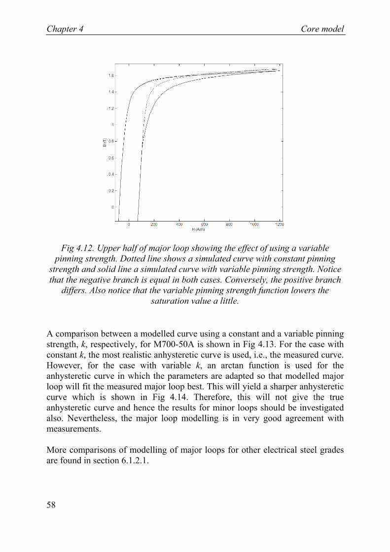
Chapter 4 Core model
58
Fig 4.12. Upper half of major loop showing the effect of using a variable
pinning strength. Dotted line shows a simulated curve with constant pinning strength and solid line a simulated curve with variable pinning strength. Notice that the negative branch is equal in both cases. Conversely, the positive branch
differs. Also notice that the variable pinning strength function lowers the saturation value a little.
A comparison between a modelled curve using a constant and a variable pinning strength, k, respectively, for M700-50A is shown in Fig 4.13. For the case with constant k, the most realistic anhysteretic curve is used, i.e., the measured curve. However, for the case with variable k, an arctan function is used for the anhysteretic curve in which the parameters are adapted so that modelled major loop will fit the measured major loop best. This will yield a sharper anhysteretic curve which is shown in Fig 4.14. Therefore, this will not give the true anhysteretic curve and hence the results for minor loops should be investigated also. Nevertheless, the major loop modelling is in very good agreement with measurements. More comparisons of modelling of major loops for other electrical steel grades are found in section 6.1.2.1.

Core model Chapter 4
59
0 0.2 0.4 0.6 0.8 1
0
0.2
0.4
0.6
0.8
1
1.2
1.4
1.6
H (kA/m)
B (T
)
Fig 4.13. Upper part of major loop for M700-50A. Solid line shows measured curve. Dashed line shows modelled curve with constant pinning strength using
the measured anhysteretic curve, whereas dotted line modelled curve with variable pinning strength and an adapted anhysteretic curve. Notice that the
major loop closes at higher amplitude than shown in this plot.
0 0.2 0.4 0.6 0.8 1 1.2 1.4 1.6 1.8 2
0
0.2
0.4
0.6
0.8
1
1.2
1.4
1.6
H (kA/m)
B (T
)
Fig 4.14. Dotted line shows the adapted anhysteretic curve for the major loop shown in Fig 4.13.

Chapter 4 Core model
60
4.1.2.5 Variable degree of reversibility The expression for the total magnetization in the original Bergqvist model, equation (4.5), assumes that the parameter c, which corresponds to the degree of reversibility of the magnetization, is constant. This means that the model assumes that the relation between the reversible and irreversible processes of the magnetization is constant for all magnetization levels. However, from the discussion in section 2.2.1.4 this assumption can not be true since the degree of reversibility varies for different magnetization levels. The degree of reversibility should vary with the magnetization and/or the applied field [49], [50]. It has also been suggested that it could also be history-dependent [50].
Engdahl [57] proposes a modification to Bergqvist’s lag model where c is dependent on the applied field. The static magnetization will then be expressed as:
[ ]( )an an λk H0
( ) ( ) ( )M c H M H M P H dς λ λ∞
= +∫ (4.19)
The expression for c (H) is then changed to:
0
an
( )( )( )Hc HH
χχ
= (4.20)
where χ0 (H) is the linear portion of the susceptibility of a curve starting from an arbitrary point, (M, H), on the anhysteretic curve and χan (H) is the susceptibility of the anhysteretic curve in that point. Now, the density function will be dependent on H:
2( ( ) ( ))
H ( ) ( )e p H q HA H λς λ − −= (4.21)
Furthermore, the parameter functions A (H), p (H) and q (H) are now given through the extensions of equations (4.8) - (4.10) in order to be valid for different H:

Core model Chapter 4
61
H0( ) 1 ( )d c Hς λ λ
∞= −∫ (4.22)
H0( ) 1dλς λ λ
∞=∫ (4.23)
2( )
H 0 01 ( )( ) (0) ( ) e ( )
2 2q HA HH H H
k kκ ς χ χ−= = (4.24)
If instead the parameter c = c (M), i.e., dependent on the magnetization, the expressions corresponding to equations (4.19) - (4.23) are obvious.
4.1.2.6 Modified play operator Bormann [58] proposes the following modified play operator:
[ ][ ] [ ]
[ ][ ]
k k
k,c k
k
if
if
if
P H c H H H P H k
P H H H H k H H P H k
H H k H H P H k
Δ Δ
Δ Δ Δ
Δ Δ
⎧⎪ + + − <⎪⎪⎪+ = + − + − ≥⎨⎪⎪⎪ + + + − ≤−⎪⎩
(4.25)
This new play operator is depicted in Fig 4.15.
The contribution of the reversible part is here introduced directly into the play operator via the parameter c. Moreover, c could in principle be an arbitrary function of M or H.

Chapter 4 Core model
62
2k
Pk
Pk,c
Fig 4.15. Play-operators. Blue, solid line shows the original operator and red, dashed line shows the new operator.
If ς(λ) is the density function which gives the weight of the pseudo particles the total magnetization can be expressed:
[ ]( )an λk,c0
( )M M P H dς λ λ∞
=∫ (4.26)
The density function is normalized through the following conditions:
0
( ) 1dς λ λ∞
=∫ (4.27)
0
( ) d kς λ λ λ∞
=∫ (4.28)

Core model Chapter 4
63
Here, k is the mean pinning strength. Now, the play operator on the major loop is given by:
[ ]k,cP H H k±= ∓ (4.29)
for the positive and negative branch, respectively. This gives the magnetization branches as:
( )an0
( )M M H k dς λ λ∞
± =∫ ∓ (4.30)
An interesting feature of equation (4.30) is that it is independent on the degree of reversibility, c. Since both functions M± and Man can be obtained from measurements it is possible to determine the distribution function, ς (λ) from this equation. For a description of this determination procedure see Appendix III.
4.2 Dynamic magnetization model
4.2.1 Cauer circuits As mentioned in section 2.2.2.1 the classical eddy currents expression, equation (2.14), is valid only if the condition in equation (2.15) is satisfied. That condition is usually satisfied for materials with a thickness of 0.1-1.0 mm up to around 100 Hz. For thinner materials the condition is valid for higher frequencies.
The sheets in a transformer core laminate have typically a thickness of 0.2-1.0 mm. This means that the field distribution inside the material will be inhomogeneous and the use of equation (2.14) introduces errors for higher frequencies. The analytical solution of this problem becomes very complex; since one has to consider that the magnetic domains in the material can exhibit different magnetization at a certain time. Furthermore, the magnetization law for the typical material has to be known, and as a result it is very difficult to derive a general model.

Chapter 4 Core model
64
Bertotti [19] derives the solutions for materials with linear or steplike magnetization laws. However the solutions are only valid under sinusoidal conditions and are therefore not useful for minor loops or other waveforms.
In this thesis a different approach called Cauer circuits [48] are used. These are circuits of ladder network type and are more commonly used in signal theory. However, they have been used earlier for modelling of magnetic cores in general [28], [52], [73], [74], [75], [76] and transformers cores in particular [8], [13], [28], [51] . Furthermore, a survey of the technique is presented in ref. [28]. More recent applications are found in refs. [53] and [54]. In this thesis the feasibility of using Cauer circuits as a part of a dynamic magnetization model will be studied.
A short resume of the Cauer circuit technique is presented below.
4.2.1.1 Modelling method When a material is exposed to a varying magnetic field, the field distribution will vary over the cross-section thickness due to the eddy current shielding effect. The governing idea of Cauer circuits is to divide the cross-section into a finite number of sections, where every section is smaller than the total thickness. This is shown in Fig 4.16. Each section carries the average field in that section. If the sections are chosen sufficiently small the field inside them is approximately uniformly distributed and so are the magnetization. This technique is often called “lumping”.
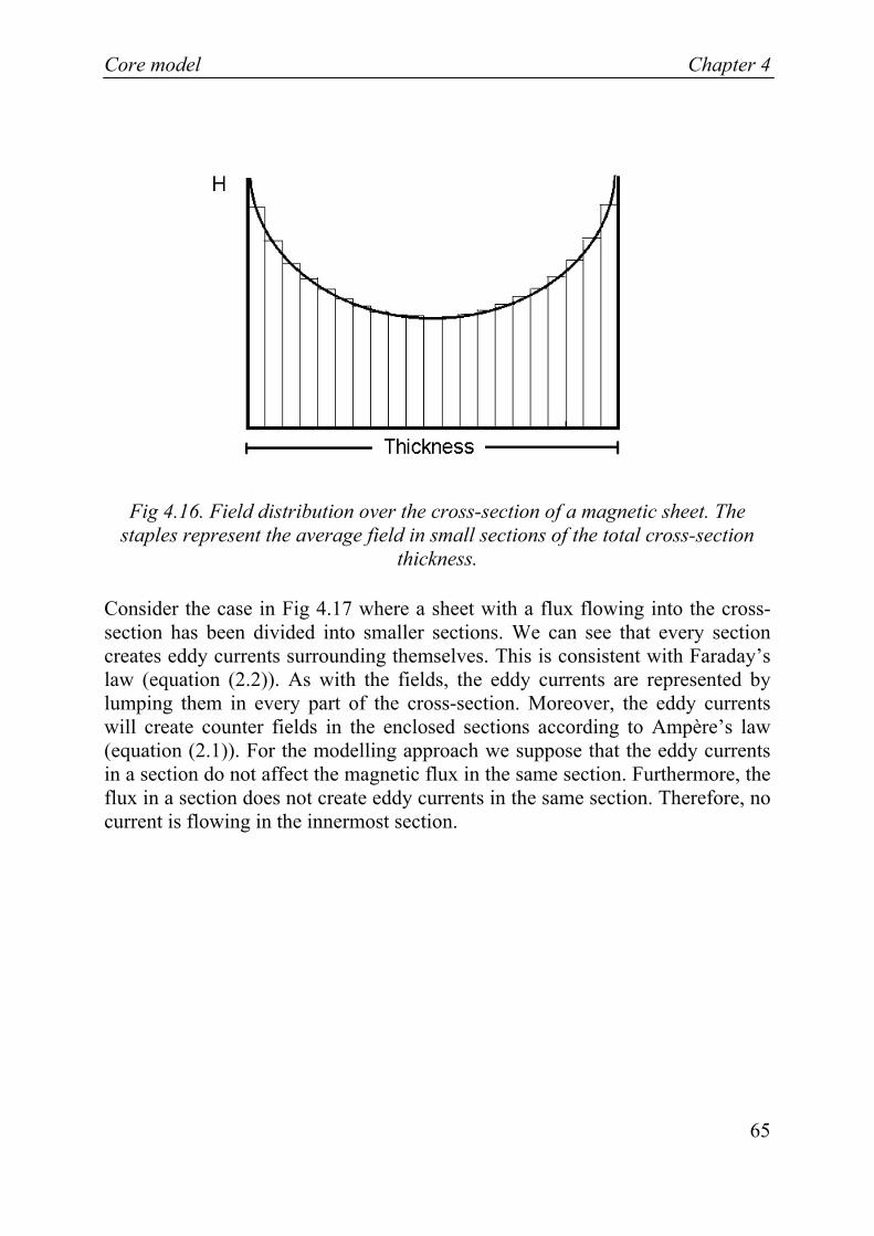
Core model Chapter 4
65
Fig 4.16. Field distribution over the cross-section of a magnetic sheet. The staples represent the average field in small sections of the total cross-section
thickness.
Consider the case in Fig 4.17 where a sheet with a flux flowing into the cross-section has been divided into smaller sections. We can see that every section creates eddy currents surrounding themselves. This is consistent with Faraday’s law (equation (2.2)). As with the fields, the eddy currents are represented by lumping them in every part of the cross-section. Moreover, the eddy currents will create counter fields in the enclosed sections according to Ampère’s law (equation (2.1)). For the modelling approach we suppose that the eddy currents in a section do not affect the magnetic flux in the same section. Furthermore, the flux in a section does not create eddy currents in the same section. Therefore, no current is flowing in the innermost section.

Chapter 4 Core model
66
Fig 4.17. A magnetic sheet divided into smaller sections. For electrical steels the width of the sheets is much larger than the thickness in order to reduce the eddy currents. This also means that the vertical parts of the currents paths are
negligible.
Now, referring to Fig 4.17, the total flux in the material can be expressed as:
tot 1 2 3 ... nϕ ϕ ϕ ϕ ϕ= + + + + (4.31)
This can be represented with the circuit illustrated in Fig 4.18 where iℜ denote the reluctances of the section of the magnetic material that is given by:
i i i i i i i i iB A H Aθ ϕ μ= ℜ =ℜ =ℜ (4.32)
i i iH lθ = (4.33)
i i i i iH l H Aμ= ℜ (4.34)
Here θi is the applied MMF (magneto motive force) and li is the magnetic path length over which Hi is applied. This finally gives:

Core model Chapter 4
67
ii
i
lAμ
ℜ = (4.35)
Equation (4.35) shows that iℜ is inversely proportional to the magnetic permeability of the material.
1ℜ 2ℜ 3ℜ nℜ
Fig 4.18. Lumping of reluctances of different sections.
The circuit shown in Fig 4.18 represents the lumping of the magnetic fluxes in the different sections of the sheet. However, we also have to represent the eddy currents. This can be done by using a so called winding component seen in Fig 4.19. The winding component realizes the relation between the magnetic flux in a material and the currents surrounding the flux, e.g., in a winding or, as in this case, a surrounding material section. In the magnetic part of the winding component a flux flows and a MMF is induced. In the electric part an EMF (electro motive force) is induced and a current flows through the resistance, R.

Chapter 4 Core model
68
NIθ = dNdtϕε = −
Fig 4.19. Winding component with the magnetic part on the left side and the electric on the right.
Using Ohm’s law in the electric part we can calculate I as:
N dIR dt
ϕ= − (4.36)
where N is the number of turns, in this case N = 1. Now, for the magnetic part we get:
2 1N d dNI
R dt R dtϕ ϕθ = = − = − (4.37)
Through the electric-magnetic analogy this equals a “magnetic” inductance with value 1/R. Inserting the magnetic inductances corresponding to the winding components, and thereby the eddy currents, into the circuit in Fig 4.18 yields the circuit depicted in Fig 4.20.

Core model Chapter 4
69
1ℜ 2ℜ 3ℜ nℜ
1
1R 2
1R 1
1nR −
Fig 4.20. Total Cauer circuit including reluctances and eddy currents in different sections. The “magnetic” inductances represent the MMF drops due to
the eddy currents in each section.
4.2.1.2 Optimization of Cauer circuit at high frequencies For correct representation of the magnetization of magnetic materials the individual size and number of sections in the Cauer circuit are important. It has been shown that using 10 sections yields good results when choosing the appropriate size of them [28], [51]. Moreover, in those models, the sizes of the subsections have been chosen to increase linearly with 30 % [51] and 40 % [28], respectively, for each section, beginning from the outmost section. For the frequency range in this work, approximately DC – 10 kHz, this approach yields satisfying results. However, one can understand that at higher frequencies, where the field will change more rapidly near the material surface, this method would be rather coarse, and can yield incorrect results.
Here a method is proposed in which the sizes of the subsections depend on the frequency of the applied field. The idea is to choose the sizes of the sections such that we get many sections in the region where the field changes fastest and thereby also is hardest to predict.
The procedure of this frequency-dependent method is as follows:
First we estimate the field distribution inside the material which is difficult to predict. It is, however, possible to derive an analytical expression for the field

Chapter 4 Core model
70
distribution in a material with constant permeability [19], [55]. Consider the cross-section of a magnetic sheet. If the sheet has thickness d and is exposed to a time-varying magnetic field, the normalized field distribution along the sheet thickness will be:
cosh(2 / ) cos(2 / )( )
cosh( ) cos( )x d x dH x γ γγ γ
+=
+, (4.38)
where x is the distance from the outer edge of the sheet thickness and γ corresponds to the degree of penetration expressed as:
f dγ πσμ= (4.39)
Here it is assumed that the permeability is constant even if it is not the case.
Next, for the frequency of interest, we pick a number of points (equal to the number of sections) of H equally distributed between the maximum value and minimum value of H over the sheet thickness. The corresponding value of x for each H-value is then picked and used as the inner boundary for each section in the Cauer circuit. There is a great advantage with this procedure especially at high frequencies where the field changes rapidly near the surface. In these cases this procedure will yield most of the sections near the surface. On the other hand, at lower frequencies where the field does not change so fast the sections will be more evenly distributed over the cross-section and the method using linearly increasing sizes can be used.
Comparisons of simulation results of the field distribution in a sheet of a typical electrical steel with μr = 5000, σ = 2 MS/m and d = 0.3 mm are shown in Fig 4.21 - Fig 4.23 The simulations were performed using Cauer circuits with the linear method (LM), with 40 % increase between each section and the frequency-dependent method (FDM), which optimizes the sizes of the sections. The applied field was sinusoidal and the amplitude of the magnetization was kept below saturation. It can be seen in the figures that at 10 kHz, LM and FDM yield approximately the same field distribution. However, when increasing frequency up to the MHz-range FDM yields much better result than LM. This is due to the fact that at these high frequencies, the eddy current shielding effect is

Core model Chapter 4
71
very high. Nevertheless, at frequencies below 10 kHz, which is what electrical steels usually are exposed to, the difference between LM and FDM is very small.
Fig 4.21. Magnetic field distribution at 10 kHz along the cross-section of a sheet of a typical electrical steel. The curves show the following methods: analytical
expression (solid) and simulations using LM (dashed) and FDM (dotted), respectively. The rings and stars show the middle point in each section,
respectively.

Chapter 4 Core model
72
Fig 4.22. Magnetic field distribution at 1 MHz along the cross-section of a sheet of a typical electrical steel. The curves show the following methods: analytical
expression (solid) and simulations using LM (dashed) and FDM (dotted), respectively. The rings and stars show the middle point in each section,
respectively.
Fig 4.23. Magnetic field distribution at 100 MHz along the cross-section of a sheet of a typical electrical steel. The curves show the following methods: analytical expression (solid) and simulations using LM (dashed) and FDM
(dotted), respectively. The rings and stars show the middle point in each section, respectively.
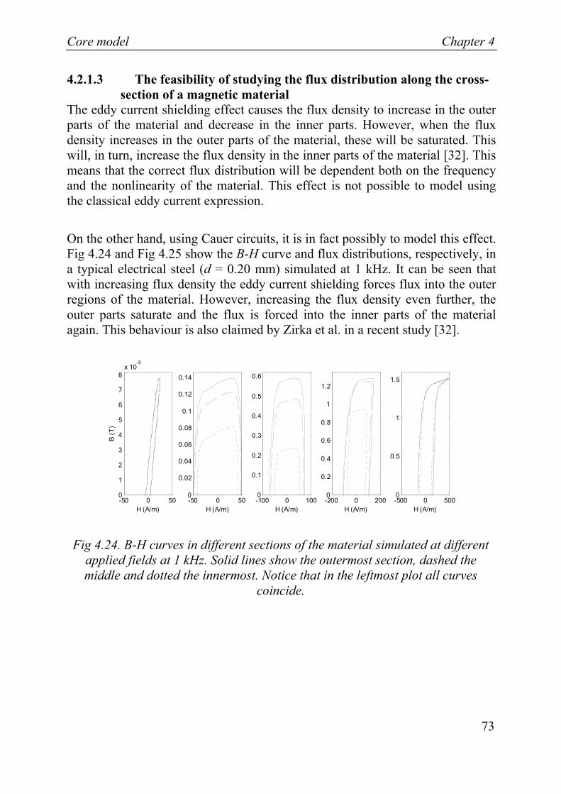
Core model Chapter 4
73
4.2.1.3 The feasibility of studying the flux distribution along the cross-section of a magnetic material
The eddy current shielding effect causes the flux density to increase in the outer parts of the material and decrease in the inner parts. However, when the flux density increases in the outer parts of the material, these will be saturated. This will, in turn, increase the flux density in the inner parts of the material [32]. This means that the correct flux distribution will be dependent both on the frequency and the nonlinearity of the material. This effect is not possible to model using the classical eddy current expression.
On the other hand, using Cauer circuits, it is in fact possibly to model this effect. Fig 4.24 and Fig 4.25 show the B-H curve and flux distributions, respectively, in a typical electrical steel (d = 0.20 mm) simulated at 1 kHz. It can be seen that with increasing flux density the eddy current shielding forces flux into the outer regions of the material. However, increasing the flux density even further, the outer parts saturate and the flux is forced into the inner parts of the material again. This behaviour is also claimed by Zirka et al. in a recent study [32].
-50 0 500
1
2
3
4
5
6
7
8x 10
-3
B (T
)
H (A/m)-500 0 5000
0.5
1
1.5
H (A/m)-200 0 2000
0.2
0.4
0.6
0.8
1
1.2
H (A/m)-50 0 500
0.02
0.04
0.06
0.08
0.1
0.12
0.14
H (A/m)-100 0 1000
0.1
0.2
0.3
0.4
0.5
0.6
H (A/m)
Fig 4.24. B-H curves in different sections of the material simulated at different applied fields at 1 kHz. Solid lines show the outermost section, dashed the middle and dotted the innermost. Notice that in the leftmost plot all curves
coincide.

Chapter 4 Core model
74
0 500 10000
1
2
3
4
5
6
7
8x 10
-3
t (us)
B (T
)
0 500 10000
0.5
1
1.5
t (us)0 500 1000
0
0.2
0.4
0.6
0.8
1
1.2
t (us)0 500 1000
0
0.02
0.04
0.06
0.08
0.1
0.12
0.14
t (us)0 500 1000
0
0.1
0.2
0.3
0.4
0.5
0.6
t (us)
Fig 4.25. Magnetic flux density in different sections of the material simulated at different applied fields at 1 kHz. Solid lines show the outermost section, dashed the middle and dotted the innermost. Notice that in the leftmost plot all curves
coincide
4.3 Composite magnetization model
The governing equation for the composite model is the expression for the total field, given in equation (2.19):
tot stat eddy excessH H H H= + + (4.40)
The total field is applied by a MMF, driving a magnetic flux through the circuit.
The field created by the eddy current, Heddy, gives a MMF drop as shown in Fig 4.20. Moreover, the field created by the excess losses, Hexcess gives a MMF drop in every reluctance element in each section individually, according to equation (2.18):
excess 04 signdB dBH GdwVdt dt
σ ⎞⎛= ⎜ ⎟⎝ ⎠
(4.41)
Here, B is the actual flux density in the actual section considered.
Core model Chapter 4
75
This gives the static part of the magnetization field, Hstat from equation (4.40). Finally, B is calculated using Bergqvist’s lag model (section 4.1.1) in every section. This means that the reluctance components in Fig 4.20 now contain the static hysteresis and the excess loss parts of the total magnetization in each section. Furthermore, the eddy current part is given by the “magnetic” inductances.
One problem with the formulations is that the static model calculates B as a function of H while the excess loss expression calculates H as a function of dB/dt. This can, however, be solved by using the value of dB/dt at the nearest previous time point, as an approximation for dB/dt at the desired time point. This requires, of course, that the time step is small enough so that the small errors introduced can be neglected.
4.3.1 Discussion An alternative for the excess loss component is to realize it as one component for the whole circuit, and not in every section. However, that approach would only manage to account for the average flux density in the material. When simulating it in every section, it is possible to account for the difference in the flux distribution, through the different flux densities in different sections, which is more physically correct.

Composite transformer model Chapter 5
77
Chapter 5
Composite transformer model
5.1 One phase
The composite transformer model consists of a winding model and core model connected together. For a one phase transformer this is achieved by attaching a winding component, comprising the features presented in Chapter 3, to a core component, comprising the features presented in Chapter 4. The interaction between the core and winding components are presented schematically in Fig 5.1. The currents in the two windings, respectively, are given through the winding module and generating an MMF in the core module. The flux in the core module, in turn, induces EMF:s in the windings. The generality of the model gives the opportunity to vary the resolution of the core and winding models individually.
In section 6.2 an one phase three leg transformer model is verified by measurements. Also different resolutions of the core and winding models are tested for frequencies up to 1000 Hz.

Chapter 5 Composite transformer model
78
Winding module
I1
I2
θ1 = N1I1
θ2 = N2I2
+
+
+
+
1 1dNdtϕε = −
2 2dNdtϕε = −
φ
Core module
V
Load
Connection to other parts of the
transformer
Connection to other parts of the
transformer
Fig 5.1. Simplified diagram of the composite transformer model comprising two winding coils, linked by a winding module, which generate MMF:s in the core. Also seen is the core module and the, by the flux in the core, induced EMF:s in
the windings.
5.2 Three phases
It is possible to connect three different legs together to constitute a three phase three leg model. Furthermore, one can connect magnetic elements between the legs to model the magnetic characteristics of the yokes and joints. Fig 5.2 illustrates the schematics of a three phase three leg transformer. As seen in the figure, three leg components are coupled together via a reluctance network with yoke and joint components. Each leg component comprises the composite core
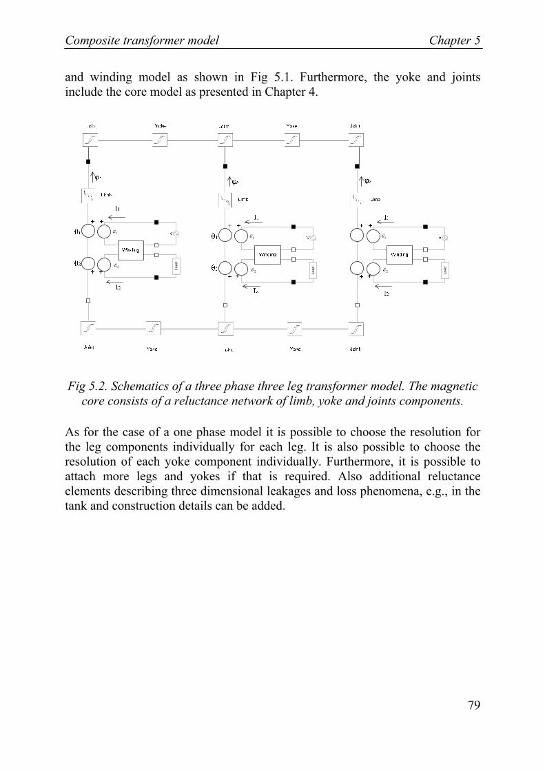
Composite transformer model Chapter 5
79
and winding model as shown in Fig 5.1. Furthermore, the yoke and joints include the core model as presented in Chapter 4.
1ε
2ε Load
1ε
2ε Load
1ε
2ε Load
Fig 5.2. Schematics of a three phase three leg transformer model. The magnetic core consists of a reluctance network of limb, yoke and joints components.
As for the case of a one phase model it is possible to choose the resolution for the leg components individually for each leg. It is also possible to choose the resolution of each yoke component individually. Furthermore, it is possible to attach more legs and yokes if that is required. Also additional reluctance elements describing three dimensional leakages and loss phenomena, e.g., in the tank and construction details can be added.


Experimental verification Chapter 6
81
Chapter 6
Experimental verification
In this chapter verifications of the magnetic core model and the composite transformer model, presented in Chapter 4 and 5 respectively, are presented. This includes verifications of the static and composite magnetization models. It also includes the verification of normal operation of a one-phase transformer model under different load conditions. Furthermore, this model is verified in no-load and non-normal operations like inrush currents and DC-magnetization.
Unfortunately, there has not been enough time to verify the detailed winding model as presented in Chapter 3. Instead a simplified winding model is used in the verification of the composite transformer model.
6.1 Core model verification
In order to verify the static and dynamic hysteresis models, a number of measurements were performed. These included measurements of static major and minor loops on electrical steels. Furthermore, dynamic measurements were performed at different frequencies and amplitudes of applied fields. The dynamic measurements were done both with controlled H- and B-field, respectively.
Thereafter, the same cases were simulated in order to verify the models. In the following section the procedure and results of the measurements and simulations are presented.

Chapter 6 Experimental verification
82
6.1.1 Static measurements
6.1.1.1 Set-up The set-up for the static measurements is as seen in Fig 6.1. The measurement is controlled from a computer, which, via a digital to analog converter (DAC), gives a voltage as input to an amplifier. The amplifier gives a current as output. The Epstein frame is a quadratic board with coils located on each side. Inside the coils flat strips of magnetic materials are placed. The current from the amplifier runs through the coils (connected in series) and creates magnetic fields along the axial direction of the strips according to Ampère’s law. There are also pickup coils (also connected in series) on each side of the frame. The pickup coils are connected to a fluxmeter, which takes the induced voltage in the coils as input and calculates the flux by Faraday’s law. Thereby, the flux density becomes:
Udt
BNA
= ∫ (6.1)
where U is the voltage over the coils, N is the number of turns of the coil and A is the cross-sectional area of the magnetic material.
Fig 6.1. Block scheme of set-up for static measurements.
In the static case the field changes so slowly that the signal from the computer can be used directly in order to give the value of the magnetic field. However, these values have to be calibrated against the real field. In order to do this the current that flows through the Epstein frames primary coil is measured. This is done with a current sensor in form of a current clamp placed around the cable
Experimental verification Chapter 6
83
between the amplifier and the Epstein frame. Knowing the number of turns in the coil the magnetic field is known by using Ampère’s law, i.e.:
NIHl
= , (6.2)
where l is the magnetic path length. In the Epstein frame used, the total number of turns is 700 both for the coils for applying the field and for the pickup coils. Moreover, the sides of the frame are 28 cm long. For the measurements, strips of magnetic materials are placed inside every coil. The strips are 28 cm long and 3 cm wide and are lapped into each other in the joints. Hereby, the effective magnetic length of each strip is only 25 cm. Furthermore, the magnetic flux will leak inside the strips in the joints and as a result the effective magnetic path length for the whole set-up is approximately 0.94 m [59].
The values of the B-field are returned back via the analog to digital converter (ADC) to the computer, where they are stored.
6.1.1.2 Major loops Static major loops of three electrical steels with different properties were measured. The applied magnetic fields were sinusoidal with frequency 1 mHz, which for the thickness of these materials are low enough to be considered as static. The following materials were measured:
• M5. Thickness 0.30 mm, width 3.0 cm, grain oriented.
• M700-50A, rolling direction. Thickness 0.50 mm, width 3.0 cm, nonoriented.
• 23ZDKH. Thickness 0.23 mm, width 3.0 cm, strongly oriented, laser-scribed*.
* As the word laser-scribe implies, a laser is used to mark dotted lines transverse to the direction of the orientation. The lines lie at a distance of a couple of centimeters and hinder the movement of domain walls when the material is exposed to a fluctuating field. This decrease the excess losses.

Chapter 6 Experimental verification
84
The measured static major loops of those steels are shown in Fig 6.2.
-800 -600 -400 -200 0 200 400 600 800
-1.5
-1
-0.5
0
0.5
1
1.5
H (A/m)
B (T
)
Fig 6.2. Static major loops for different electrical steels. Dashed line shows 23ZDKH, solid line shows M5 whereas dotted line shows M700-50A.
6.1.1.3 Minor loops In section 4.1.2.1 a demagnetization curve was shown for M700-50A, see Fig 4.3.. Many of the loops in that curve were closed or nearly closed. Some of these loops were extracted in order to use for verification of the core model. These loops are shown in Fig 6.3.

Experimental verification Chapter 6
85
-0.2 -0.15 -0.1 -0.05 0 0.05 0.1 0.15 0.2-1.5
-1
-0.5
0
0.5
1
1.5
H (kA/m)
B (T
)
Fig 6.3. Minor loops for M700-50A extracted from demagnetization curve.
6.1.2 Static simulations In this section results from simulations of major and minor loops of the material presented in the previous section are shown. These static simulations were executed in Matlab*. Firstly, simulations of major loops for three electrical steels are presented. Then, an example of simulations of minor loops is shown.
* www.matlab.com

Chapter 6 Experimental verification
86
6.1.2.1 Major loops The major loops of the three materials shown in Fig 6.2 were used as a starting point. Thereafter, it was tried to replicate these major loops as good as possible by simulations. For best possible fitting of the shapes of the loops (judged visually), the logarithmic modified arctan function shown in equation (4.17) was used together with the expression for the variable pinning strength in equation (4.18). As shown in Fig 4.13 this technique is able to yield a better fit for the major loop then using the measured anhysteretic curve. The reason for this is that the variable pinning strength was used together with the arctan function, but not with the measured anhysteretic curve. Therefore, the arctan function yields better fit for the whole major loop and was therefore used in the simulations.
In order to replicate the measured curves as good as possible the parameters in equation (4.17) and (4.18) were adapted in the simulations. This was done manually. Results for the simulation of the major loops of the three materials are shown in Fig 6.4 - Fig 6.6. The values of the adapted parameters are shown in Table 6.1 Notice that the Langevin function and other appropriate mathematical functions using the same modifications as for the arctan function is considered to yield equal results.

Experimental verification Chapter 6
87
0 100 200 300 400 500 600 700 800 900 1000
0
0.2
0.4
0.6
0.8
1
1.2
1.4
1.6
H (A/m)
B (T
)
Fig 6.4. Upper half of major loop for M700-50A. Solid line shows the measured curve and dashed line the best fitted curve from simulations.
Fig 6.5. Upper half of hysteresis loop for M5. Solid line shows the measured curve and dashed line the best fitted curve from simulations.
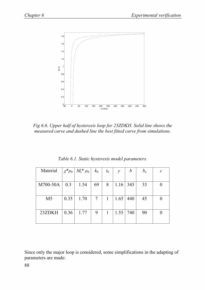
Chapter 6 Experimental verification
88
-50 0 50 100 150 200 250 300 350 400 450 5000
0.2
0.4
0.6
0.8
1
1.2
1.4
1.6
1.8
H (A/m)
B (T
)
Fig 6.6. Upper half of hysteresis loop for 23ZDKH. Solid line shows the measured curve and dashed line the best fitted curve from simulations.
Table 6.1. Static hysteresis model parameters.
Material χ*μ0 Ms* μ0 k0 t0 y b be c
M700-50A 0.3 1.54 69 8 1.16 345 33 0
M5 0.35 1.70 7 1 1.65 440 45 0
23ZDKH 0.36 1.77 9 1 1.55 740 90 0
Since only the major loop is considered, some simplifications in the adapting of parameters are made:
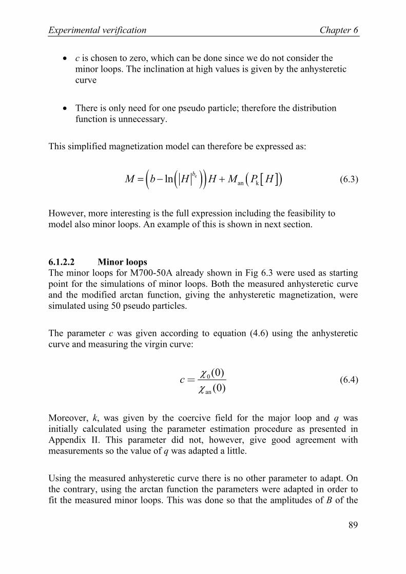
Experimental verification Chapter 6
89
• c is chosen to zero, which can be done since we do not consider the minor loops. The inclination at high values is given by the anhysteretic curve
• There is only need for one pseudo particle; therefore the distribution function is unnecessary.
This simplified magnetization model can therefore be expressed as:
( )( ) [ ]( )e
an kln bM b H H M P H= − + (6.3)
However, more interesting is the full expression including the feasibility to model also minor loops. An example of this is shown in next section.
6.1.2.2 Minor loops The minor loops for M700-50A already shown in Fig 6.3 were used as starting point for the simulations of minor loops. Both the measured anhysteretic curve and the modified arctan function, giving the anhysteretic magnetization, were simulated using 50 pseudo particles.
The parameter c was given according to equation (4.6) using the anhysteretic curve and measuring the virgin curve:
0
an
(0)(0)
c χχ
= (6.4)
Moreover, k, was given by the coercive field for the major loop and q was initially calculated using the parameter estimation procedure as presented in Appendix II. This parameter did not, however, give good agreement with measurements so the value of q was adapted a little.
Using the measured anhysteretic curve there is no other parameter to adapt. On the contrary, using the arctan function the parameters were adapted in order to fit the measured minor loops. This was done so that the amplitudes of B of the
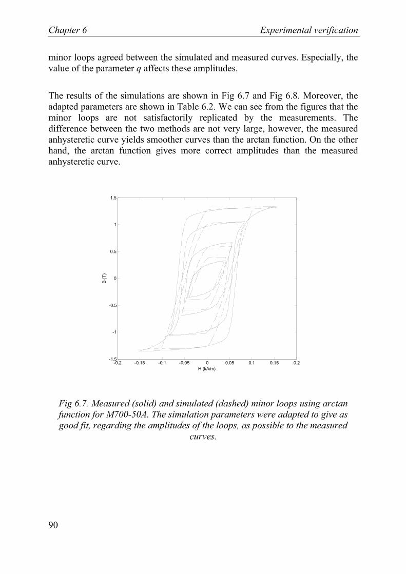
Chapter 6 Experimental verification
90
minor loops agreed between the simulated and measured curves. Especially, the value of the parameter q affects these amplitudes.
The results of the simulations are shown in Fig 6.7 and Fig 6.8. Moreover, the adapted parameters are shown in Table 6.2. We can see from the figures that the minor loops are not satisfactorily replicated by the measurements. The difference between the two methods are not very large, however, the measured anhysteretic curve yields smoother curves than the arctan function. On the other hand, the arctan function gives more correct amplitudes than the measured anhysteretic curve.
-0.2 -0.15 -0.1 -0.05 0 0.05 0.1 0.15 0.2-1.5
-1
-0.5
0
0.5
1
1.5
H (kA/m)
B (T
)
Fig 6.7. Measured (solid) and simulated (dashed) minor loops using arctan function for M700-50A. The simulation parameters were adapted to give as good fit, regarding the amplitudes of the loops, as possible to the measured
curves.

Experimental verification Chapter 6
91
-0.2 -0.15 -0.1 -0.05 0 0.05 0.1 0.15 0.2-1.5
-1
-0.5
0
0.5
1
1.5
H (kA/m)
B (T
)
Fig 6.8. Measured (solid) and simulated (dashed) minor loops using the measured anhysteretic curve for M700-50A. The simulation parameters were
adapted to give as good fit, regarding the amplitudes of the loops, as possible to the measured curves.
Table 6.2. Adapted parameters for minor loops simulations of M700-50A.
Anhysteretic curve
χ*μ0 Ms* μ0 k0 t0 y b be c q
Modified arctan
0.8 1.64 69 0 1.5 200 15 0.01 1
Measured - - 69 - - - - 0.01 0

Chapter 6 Experimental verification
92
In the simulations of the minor loops the parameters c is very small, almost zero. Furthermore, setting it to zero did not change the results noticeable.
6.1.2.3 Discussion In this thesis the parameter values of the static model has been adapted such that the simulated curves fit the measured curves. This raises the questions how to determine the parameter values and how to evaluate the best fit.
Three different methods to determine the parameter values were tested:
1) Using the procedure proposed in Appendix II.
2) Using an algorithm that iteratively adapts the values in order to minimize the area between simulated and measured curves of a branch of the major loop and the virgin curve, respectively. This algorithm was created by Dr. Julius Krah [86].
3) Adapting the values manually to fit the shapes of major loop and minor loops.
None of these methods were able to yield a good fit both for minor and major loops. This recalls the need of modifying the static model for minor loops. Especially, the description of the parameter c should be modified, e.g., as proposed in section 4.1.2.5 and 4.1.2.6.
On the other hand, it was possible to yield a good fit for the major loop using the third of the above listed methods and fitting only the major loop.
In order to evaluate the best fit there are different possibilities. The fact that the materials saturate means that the slope of the curve changes rapidly. One possibility is to judge the fit visually. Another possibility is to use a least-square method to minimize the error. A third possibility is to minimize the area between the simulated and measured curves. In order to do this the total area has to be divided into smaller elements. A fourth possibility, if the magnetization curve follows a closed loop, is to fit the area of the loop.

Experimental verification Chapter 6
93
Fitting visually requires careful examination of the simulated results not to introduce errors, however, can yield very good fit and be performed in a short time. A least-square method requires an adequate description of which residuals to minimize. If one can achieve that this method is fast and can be exact. The method of minimizing the areas between the simulated and measured curves requires an adequate weighting of the different area elements. Finally, fitting the area of the loop is easy, however, can yield simulated curve shapes that do not fit the measured curve shapes.
In this section the parameter values have been adapted manually in order to fit the shapes of simulated curves to the measured. This was done since this was a fast method and did yield good correspondence with measured curves especially for the major loops. For the simulations of the minor loops it was not possible to achieve good fit for all loops simultaneously. Therefore, the parameter values were chosen such that the amplitudes between simulations and measurements agreed as good as possible. The judging of the fitting was done visually.
6.1.3 Dynamic measurements with controlled H-field
6.1.3.1 Set-up For the dynamic measurements with controlled H-field another set-up than in the static case was used. The problem with the Epstein frame is that the large number of coil turns and the amount of magnetic materials imply a large inductance. Moreover, this inductance is strongly nonlinear due to the hysteresis effect.
Therefore, a single sheet tester (SST) which has a much smaller inductance was used. The SST used was presented in ref. [42]. It consists of two equal U-shaped yokes placed above each other, as shown in Fig 6.9. It was originally designed as a two dimensional measurements set-up (Rotational SST) with another yoke pair placed perpendicularly to and inside the first two yokes. Each yoke is encircled by a coil and the coils of both halves are connected in series which creates a magnetic field in the yokes. The magnetic field will drive a flux through the yokes, which are made of laminated steel, and the directions of the fluxes from the two yokes are so that they oppose each other where the yokes meet. Thereby, the flux is forced to return through the air window between the yokes. By placing a magnetic sheet between the yokes running from one side to

Chapter 6 Experimental verification
94
the other side, the flux will mainly flow in the material, since its permeability is much higher there than in the air. The number of turns is 50 for each coil and the horizontal distance between the yokes is 9.0 cm. For more information about the SST see ref. [42].
Fig 6.9. Cross-sectional view of a SST.
The set-up used is shown in Fig 6.10. Again, the computer gives the output signal to a DAC, which in turn provides the amplifier with a voltage. The amplifier drives a current through the coils in the SST. Inside the SST a strip of a magnetic material is placed. For measurement of the flux density a coil is surrounding the strip. The voltage over the coil is measured by a fluxmeter and the flux density is calculated in the same way as for the static set-up. For measurement of the field a Hall probe is placed as close as possible to the surface of the material. The Hall probe measures the drift of the electrons caused by the magnetic field. This probe is attached to a gaussmeter which calculates the field. Using the ADC the values of the flux density and field are provided to the computer which stores them. More information about these measurements is found in Appendix IV.
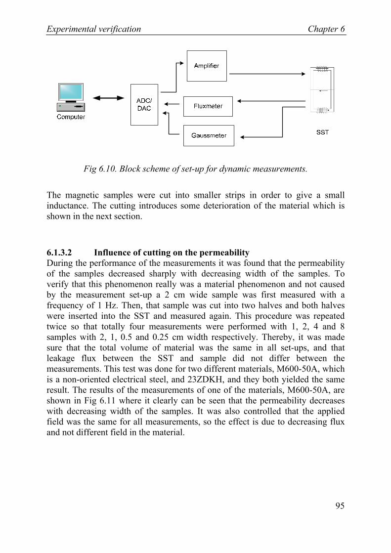
Experimental verification Chapter 6
95
Fig 6.10. Block scheme of set-up for dynamic measurements.
The magnetic samples were cut into smaller strips in order to give a small inductance. The cutting introduces some deterioration of the material which is shown in the next section.
6.1.3.2 Influence of cutting on the permeability During the performance of the measurements it was found that the permeability of the samples decreased sharply with decreasing width of the samples. To verify that this phenomenon really was a material phenomenon and not caused by the measurement set-up a 2 cm wide sample was first measured with a frequency of 1 Hz. Then, that sample was cut into two halves and both halves were inserted into the SST and measured again. This procedure was repeated twice so that totally four measurements were performed with 1, 2, 4 and 8 samples with 2, 1, 0.5 and 0.25 cm width respectively. Thereby, it was made sure that the total volume of material was the same in all set-ups, and that leakage flux between the SST and sample did not differ between the measurements. This test was done for two different materials, M600-50A, which is a non-oriented electrical steel, and 23ZDKH, and they both yielded the same result. The results of the measurements of one of the materials, M600-50A, are shown in Fig 6.11 where it clearly can be seen that the permeability decreases with decreasing width of the samples. It was also controlled that the applied field was the same for all measurements, so the effect is due to decreasing flux and not different field in the material.

Chapter 6 Experimental verification
96
-1000 -500 0 500 1000
-1.5
-1
-0.5
0
0.5
1
1.5
Magnetic field strength (A/m)
Mag
netic
flux
den
sity
(T)
2 cm1 cm0.5 cm0.25 cm
Fig 6.11. Major hysteresis loops for different sample width of M600-50A. The figure clearly shows that the permeability decreases with decreasing width.
The same phenomenon has been found for electrical steel in [61], [62] and [63] where it is shown that the cause of the decrease in permeability is due to the cutting of the material. In the cutting process the material is permanently deformed by mechanical stress close to the cutting edge in such a way that the magnetic properties are deteriorated. The deterioration can be present up to 10 mm from the edge [62]. One can easily understand that the effect of the deterioration on the measured permeability increases with decreasing width of the material.
There are at least two ways to decrease this deterioration:
1) heating of the material after the cutting to a certain temperature where recrystallization occurs [62], [63]. This is called stress-relief annealing.
2) use of waterjet cutting instead of mechanical [47]
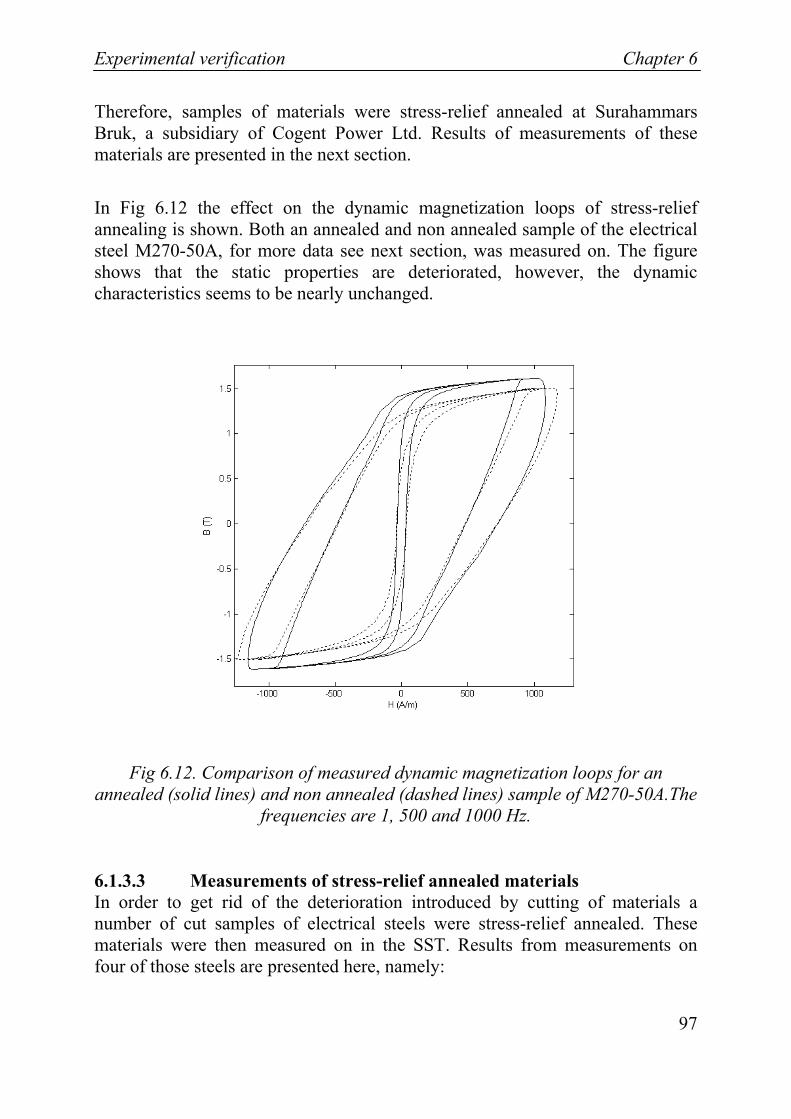
Experimental verification Chapter 6
97
Therefore, samples of materials were stress-relief annealed at Surahammars Bruk, a subsidiary of Cogent Power Ltd. Results of measurements of these materials are presented in the next section.
In Fig 6.12 the effect on the dynamic magnetization loops of stress-relief annealing is shown. Both an annealed and non annealed sample of the electrical steel M270-50A, for more data see next section, was measured on. The figure shows that the static properties are deteriorated, however, the dynamic characteristics seems to be nearly unchanged.
Fig 6.12. Comparison of measured dynamic magnetization loops for an annealed (solid lines) and non annealed (dashed lines) sample of M270-50A.The
frequencies are 1, 500 and 1000 Hz.
6.1.3.3 Measurements of stress-relief annealed materials In order to get rid of the deterioration introduced by cutting of materials a number of cut samples of electrical steels were stress-relief annealed. These materials were then measured on in the SST. Results from measurements on four of those steels are presented here, namely:

Chapter 6 Experimental verification
98
• M5, grain oriented. Thickness 0.30 mm, width 8.4 mm. Conductivity 2.08*106 S/m
• NO20, thin non-oriented. Thickness 0.20 mm, width 6.3 mm. Conductivity 1.96*106 S/m.
• M0-H, grain oriented. Thickness 0.27 mm, width 8.4 mm. Conductivity 2.09*106 S/m.
• M270-50A, non-oriented. Thickness 0.50 mm, width 6.3 mm. Conductivity 1.82*106 S/m.
Samples of the above listed materials were inserted into the SST and dynamic magnetization loops were measured at the following frequencies: 1, 50, 500, 1000 and 2000 Hz. The applied H-field was sinusoidal.
The magnetization loops of M5 at different frequencies are shown in Fig 6.13. Notice that the sampling frequency was limited. The effect of this is especially seen at 2000 Hz where the curve has sharp corners when going in and out of saturation, respectively. In reality, these corners are smooth. With at higher sampling frequency this would be seen in the measurements as well. More information about the sampling frequency is found in Appendix IV.
The loops of the other materials are shown in the verification section 6.1.5.
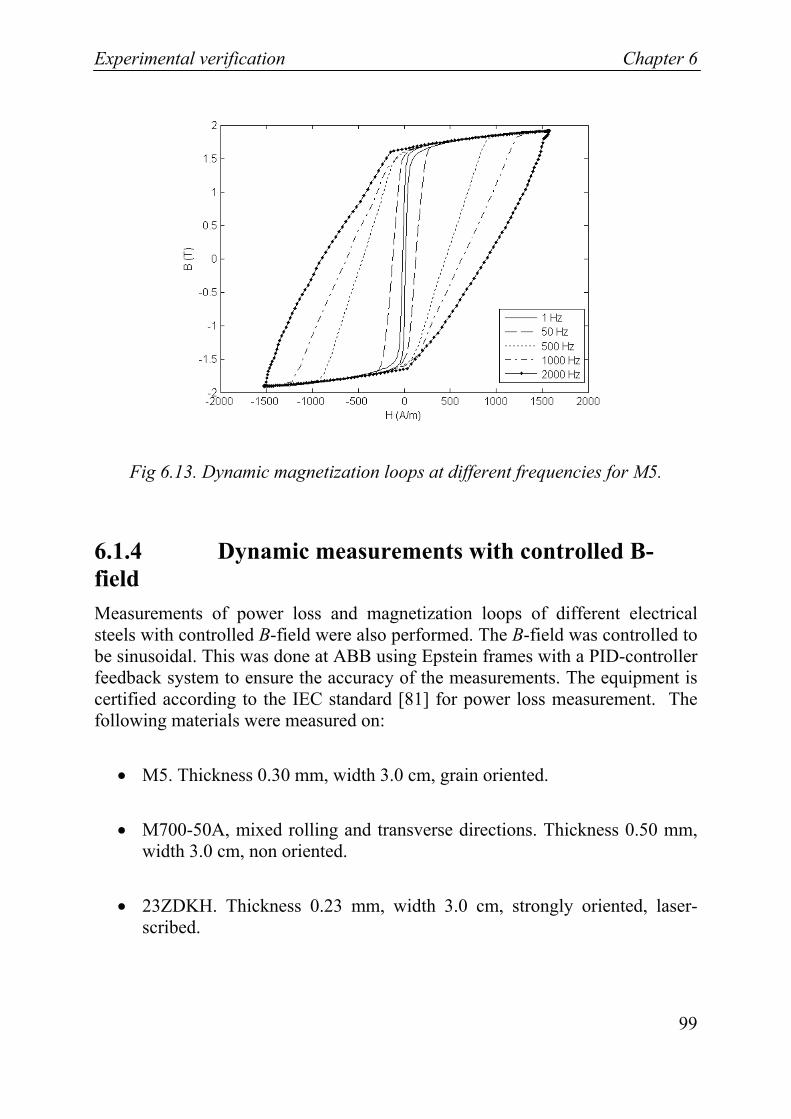
Experimental verification Chapter 6
99
Fig 6.13. Dynamic magnetization loops at different frequencies for M5.
6.1.4 Dynamic measurements with controlled B-field Measurements of power loss and magnetization loops of different electrical steels with controlled B-field were also performed. The B-field was controlled to be sinusoidal. This was done at ABB using Epstein frames with a PID-controller feedback system to ensure the accuracy of the measurements. The equipment is certified according to the IEC standard [81] for power loss measurement. The following materials were measured on:
• M5. Thickness 0.30 mm, width 3.0 cm, grain oriented.
• M700-50A, mixed rolling and transverse directions. Thickness 0.50 mm, width 3.0 cm, non oriented.
• 23ZDKH. Thickness 0.23 mm, width 3.0 cm, strongly oriented, laser-scribed.
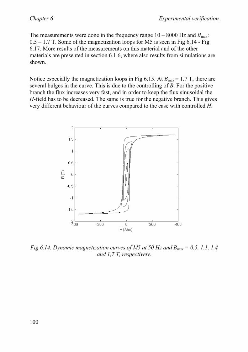
Chapter 6 Experimental verification
100
The measurements were done in the frequency range 10 – 8000 Hz and Bmax: 0.5 – 1.7 T. Some of the magnetization loops for M5 is seen in Fig 6.14 - Fig 6.17. More results of the measurements on this material and of the other materials are presented in section 6.1.6, where also results from simulations are shown.
Notice especially the magnetization loops in Fig 6.15. At Bmax = 1.7 T, there are several bulges in the curve. This is due to the controlling of B. For the positive branch the flux increases very fast, and in order to keep the flux sinusoidal the H-field has to be decreased. The same is true for the negative branch. This gives very different behaviour of the curves compared to the case with controlled H.
Fig 6.14. Dynamic magnetization curves of M5 at 50 Hz and Bmax = 0.5, 1.1, 1.4 and 1,7 T, respectively.
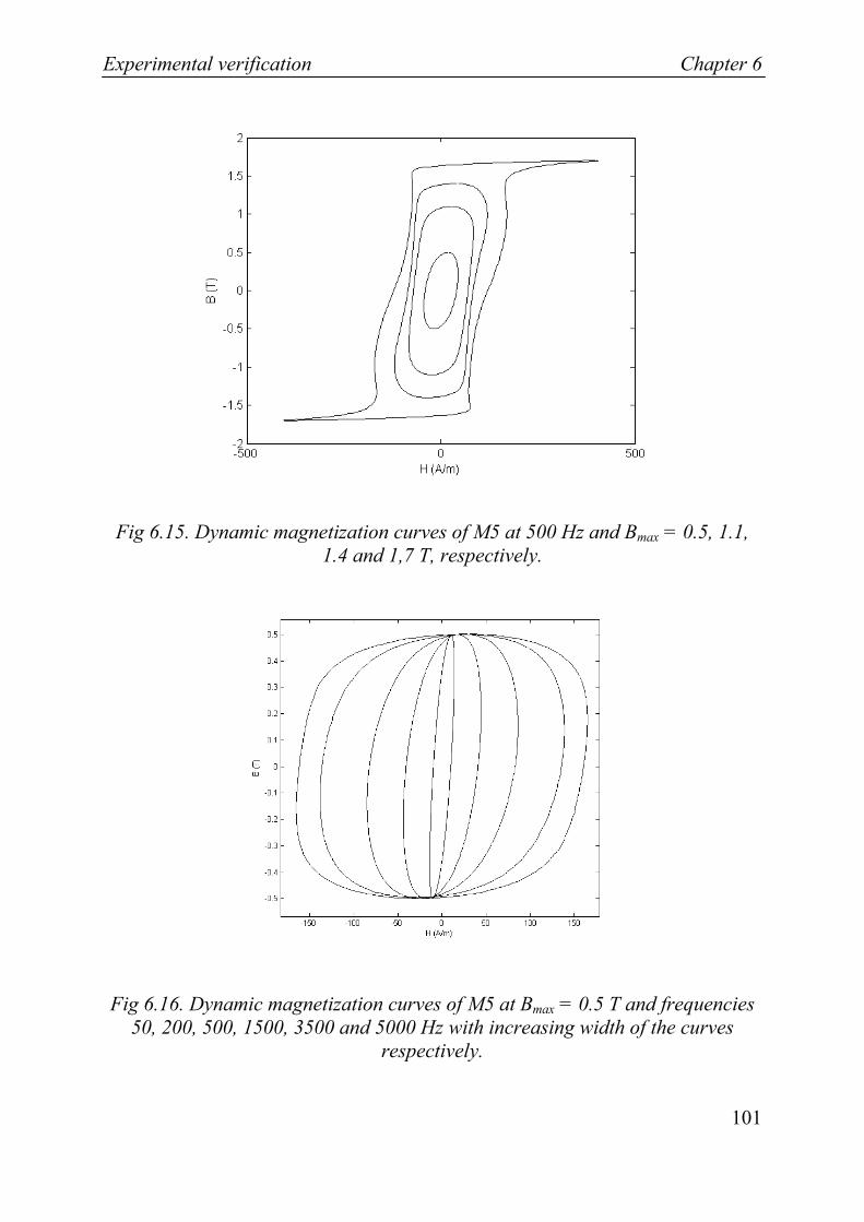
Experimental verification Chapter 6
101
Fig 6.15. Dynamic magnetization curves of M5 at 500 Hz and Bmax = 0.5, 1.1, 1.4 and 1,7 T, respectively.
Fig 6.16. Dynamic magnetization curves of M5 at Bmax = 0.5 T and frequencies 50, 200, 500, 1500, 3500 and 5000 Hz with increasing width of the curves
respectively.

Chapter 6 Experimental verification
102
Fig 6.17. Dynamic magnetization curves of M5 at Bmax = 1.7 T and frequencies 50, 200, 500 and 800 Hz with increasing width of the curves respectively
6.1.5 Dynamic simulations with controlled H-field In order to verify the dynamic magnetization model presented in section 4.3, simulations of the measured materials were performed in Dymola*. First, the cases with controlled H-field were simulated.
Simulations using the Cauer circuit model were performed for the stress-relieved materials in section 6.1.3.3. The results of this are shown in section 6.1.5.2. In order to compare the results of the model the materials were also simulated using the classical eddy current expression instead of Cauer circuits. The results of this are presented in section 6.1.5.3.
* Dymola – Dynamic Modeling Laboratory, Dynasim AB, Sweden. www.dynasim.se

Experimental verification Chapter 6
103
6.1.5.1 Simulation procedure In the measurements sinusoidal H-fields were applied and to ensure that the same waveforms were used in the simulations, the measured values of H were used as input in the simulations.
For the excess loss term (equation (2.18), all parameters are known except G and V0. The value of G is dependent on the magnetic domain structure of the material. According to ref. [19] G has a theoretically value of 0.1357 for the stripe domain structure present in electrical steels.
This leaves us with the phenomenological parameter V0. Since this parameter is a statistical parameter it is difficult (or impossible) to measure directly for these materials. However, if the assumption in ref. [44] that V0 is dependent only on the peak magnetization and not the waveform or frequency, holds, it is possible to adapt the simulated curves to the measured curves and thereby find its value.
Therefore, in this case, V0 was adapted so that the simulated magnetization curve at 50 Hz and the measured curve at the same frequency had the same energy loss for one loop. The same value of V0 was then used for the other frequencies. For the static contribution to the magnetization, the static model is adapted to the measured curves at 1 Hz. This is an approximation, however, the dynamic contribution at this frequency is very small and therefore this approximation only introduces small errors.
6.1.5.2 Simulations using Cauer circuits According to the discussion in section 4.2.1.2 it is necessary to decide how many sections to use in the Cauer circuit. In the case of simulations of sinusoidal H the curves are quite smooth and therefore the linear approach can be used. Here, it is done with 10 section and 40 % increase between each section. Conversely, when simulating with sinusoidal B the optimized approach may be needed as is shown in section 6.1.6.
The values of V0 found by fitting the simulation curve at 50 Hz to the measured curve at 50 Hz were:
• M5: V0 = 0.9 A/m
• NO20: V0 = 0.7 A/m

Chapter 6 Experimental verification
104
• M0-H: V0 = 0.8 A/m
• M270-50A: V0 = 0.3 A/m
The dynamic magnetization loops of these materials are seen in Fig 6.18 - Fig 6.21. The simulated curves follow the measured curves satisfyingly near the knees of the loops. However, close to the magnetization knee the simulated curves are sharper than the measured. Nevertheless, they replicate the shapes of the measured curves very good.
Fig 6.18. Measured (solid lines) and simulated (dashed lines) dynamic magnetization loops for M5. For the simulated results the eddy currents have
been simulated using Cauer circuits. Frequencies: 1, 50, 500, 1000 and 2000 Hz respectively with increasing width of the loops.
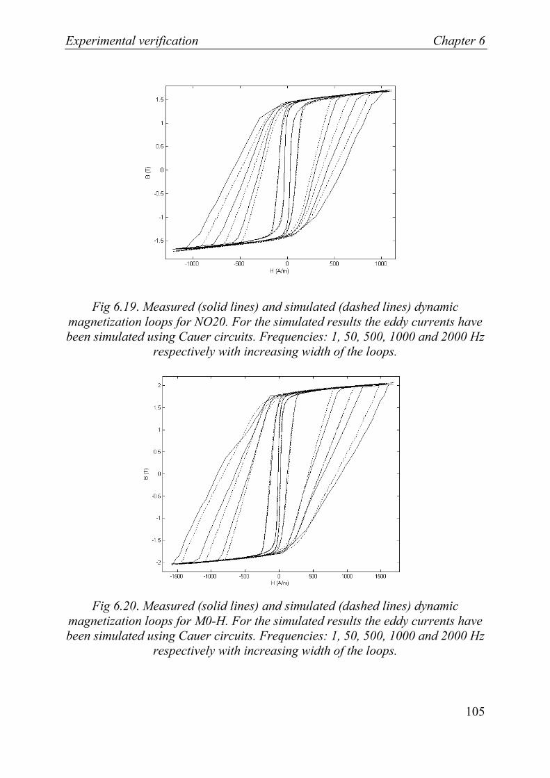
Experimental verification Chapter 6
105
Fig 6.19. Measured (solid lines) and simulated (dashed lines) dynamic magnetization loops for NO20. For the simulated results the eddy currents have been simulated using Cauer circuits. Frequencies: 1, 50, 500, 1000 and 2000 Hz
respectively with increasing width of the loops.
Fig 6.20. Measured (solid lines) and simulated (dashed lines) dynamic
magnetization loops for M0-H. For the simulated results the eddy currents have been simulated using Cauer circuits. Frequencies: 1, 50, 500, 1000 and 2000 Hz
respectively with increasing width of the loops.

Chapter 6 Experimental verification
106
Fig 6.21. Measured (solid lines) and simulated (dashed lines) dynamic
magnetization loops for M270-50A. For the simulated results the eddy currents have been simulated using Cauer circuits. Frequencies: 1, 50, 500, 1000 and
2000 Hz respectively with increasing width of the loops.
6.1.5.3 Simulations using the classical eddy currents expression The samples were also simulated using the classical eddy current expression instead of Cauer circuits as comparison. The values of V0 found by fitting the simulation curve at 50 Hz to the measured curve at 50 Hz were in this case:
• M5: V0 = 0.6 A/m
• NO20: V0 = 0.4 A/m
• M0-H: V0 = 0.5 A/m
• M270-50A: V0 = 0.01 A/m
Studying the magnetizations curves for the materials, shown Fig 6.22 - Fig 6.25, it is seen that with increasing frequency the eddy current expression becomes erroneous. This method is not capable of following the shapes of the curves,

Experimental verification Chapter 6
107
except maybe for N020, which also is the thinnest material and thereby has the least eddy current loss.
Notice also that the adapted values of V0 become lower for the method using the classical eddy current expression compared to the Cauer circuit method. This is due to the fact that the classical expression overestimates the eddy current loss and in order to compensate for that, the calculated value of the excess loss must be lower.
Fig 6.22. Measured (solid lines) and simulated (dashed lines) dynamic
magnetization loops using the classical eddy current expression for M5. Frequencies: 1, 50, 500, 1000 and 2000 Hz respectively with increasing width of
the loops.

Chapter 6 Experimental verification
108
Fig 6.23. Measured (solid lines) and simulated (dashed lines) dynamic
magnetization loops using the classical eddy current expression for NO20. Frequencies: 1, 50, 500, 1000 and 2000 Hz respectively with increasing width of
the loops.
Fig 6.24. Measured (solid lines) and simulated (dashed lines) dynamic
magnetization loops using the classical eddy current expression for M0-H Frequencies: 1, 50, 500, 1000 and 2000 Hz respectively with increasing width of
the loops.
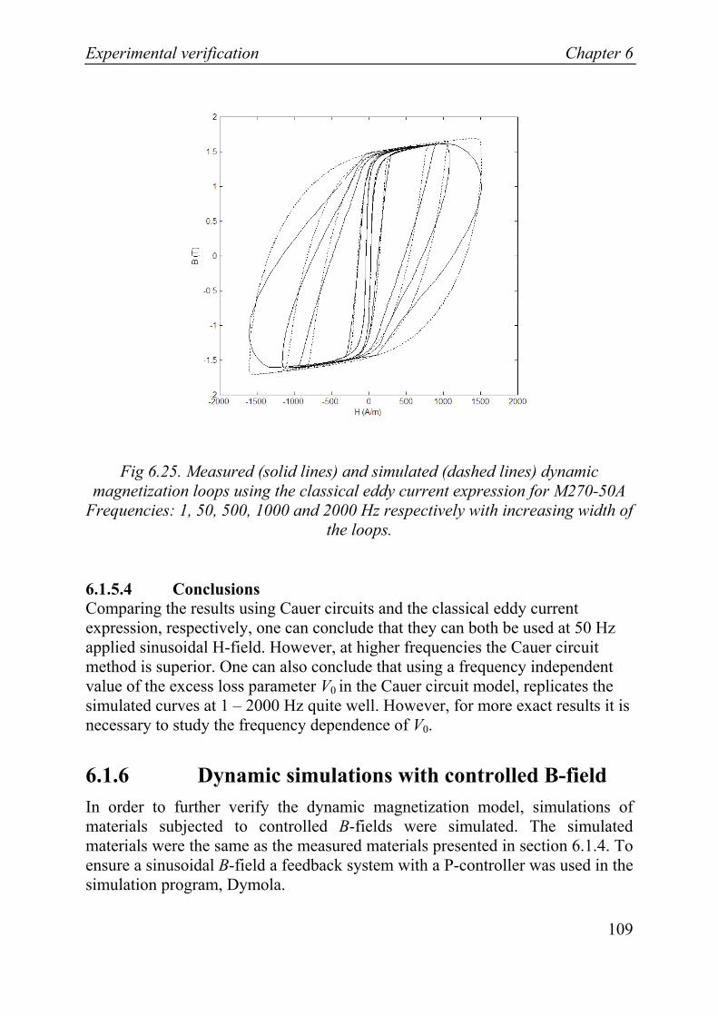
Experimental verification Chapter 6
109
Fig 6.25. Measured (solid lines) and simulated (dashed lines) dynamic magnetization loops using the classical eddy current expression for M270-50A
Frequencies: 1, 50, 500, 1000 and 2000 Hz respectively with increasing width of the loops.
6.1.5.4 Conclusions Comparing the results using Cauer circuits and the classical eddy current expression, respectively, one can conclude that they can both be used at 50 Hz applied sinusoidal H-field. However, at higher frequencies the Cauer circuit method is superior. One can also conclude that using a frequency independent value of the excess loss parameter V0 in the Cauer circuit model, replicates the simulated curves at 1 – 2000 Hz quite well. However, for more exact results it is necessary to study the frequency dependence of V0.
6.1.6 Dynamic simulations with controlled B-field In order to further verify the dynamic magnetization model, simulations of materials subjected to controlled B-fields were simulated. The simulated materials were the same as the measured materials presented in section 6.1.4. To ensure a sinusoidal B-field a feedback system with a P-controller was used in the simulation program, Dymola.

Chapter 6 Experimental verification
110
In order to get a good fit between simulated and measured curves the parameter V0 was adapted. In the case with sinusoidal H-field it was shown that adapting V0 at a low frequency yielded to low loss at higher frequencies. Therefore, in this case V0 was adapted for every frequency and amplitude of B so that the energy loss was the same in the simulated and measured case.
For the static part of the composite magnetization model, static major loops were measured for each material and the static model was adapted to these curves according to section 6.1.2. In order to model the minor loops correctly the parameters q and c in the static model were adapted to give as good agreement as possible with the measured minor loop with same amplitude.
However, since there can be a small difference between the simulated loops and the measured, this difference was compensated for. E.g. if the simulated static loss for one certain amplitude was higher than the measured loss for the same amplitude, the difference was subtracted from the simulated result of the total loss. This was done since the parameter V0 was adapted to the measured loss value. Otherwise the adapted value of V0 would be too high.
Three methods were compared:
• Linear Cauer circuit, 10 regions and 40 % increase in size between every region.
• Optimized Cauer circuit, according to section 4.2.1.2.
• Use of classical eddy current expression instead of Cauer circuits.
Furthermore, increasing the number of regions in the Cauer circuits were tested, however, the improvements were negligible. For the eddy current expression method the values of V0 were found by using equation (2.20).
The optimization of the Cauer circuit requires determination of the degree of penetration, equation (4.39). For each material the highest degree of penetration was calculated, using the highest measured frequency and highest permeability in the static major loop in the materials, i.e. the mean value between the magnetization knees. This is an approximation, however, equation (4.39), is also

Experimental verification Chapter 6
111
an approximation since it does not consider saturation and nonlinear magnetization.
In Fig 6.26 - Fig 6.29, examples of comparison between simulated and measured magnetization curves at different frequencies and Bmax = 1.7 T are shown. These cases are very interesting since they include bulges in the curves, which makes them much more difficult to simulate than straight curves. The figures show that the model replicates the simulated curves quite well for all material. In particular, the simulations of M700-50A and M5 agree well with the measurements. Moreover, for these materials the linear and optimized Cauer circuits show almost the same results. Conversely, for 23ZDKH it is seen that the optimized circuit yields much better results than the linear circuit.
It is also seen in the figures that the classical eddy current method is inferior for these cases.
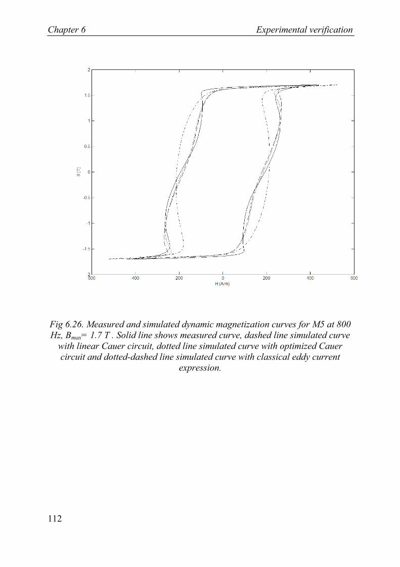
Chapter 6 Experimental verification
112
Fig 6.26. Measured and simulated dynamic magnetization curves for M5 at 800 Hz, Bmax= 1.7 T . Solid line shows measured curve, dashed line simulated curve
with linear Cauer circuit, dotted line simulated curve with optimized Cauer circuit and dotted-dashed line simulated curve with classical eddy current
expression.

Experimental verification Chapter 6
113
Fig 6.27. Measured and simulated dynamic magnetization curves for M700-50A at 800 Hz, Bmax= 1.7 T. Solid line shows measured curve, dashed line simulated
curve with linear Cauer circuit, dotted line simulated curve with optimized Cauer circuit and dotted-dashed line simulated curve with classical eddy
current expression.
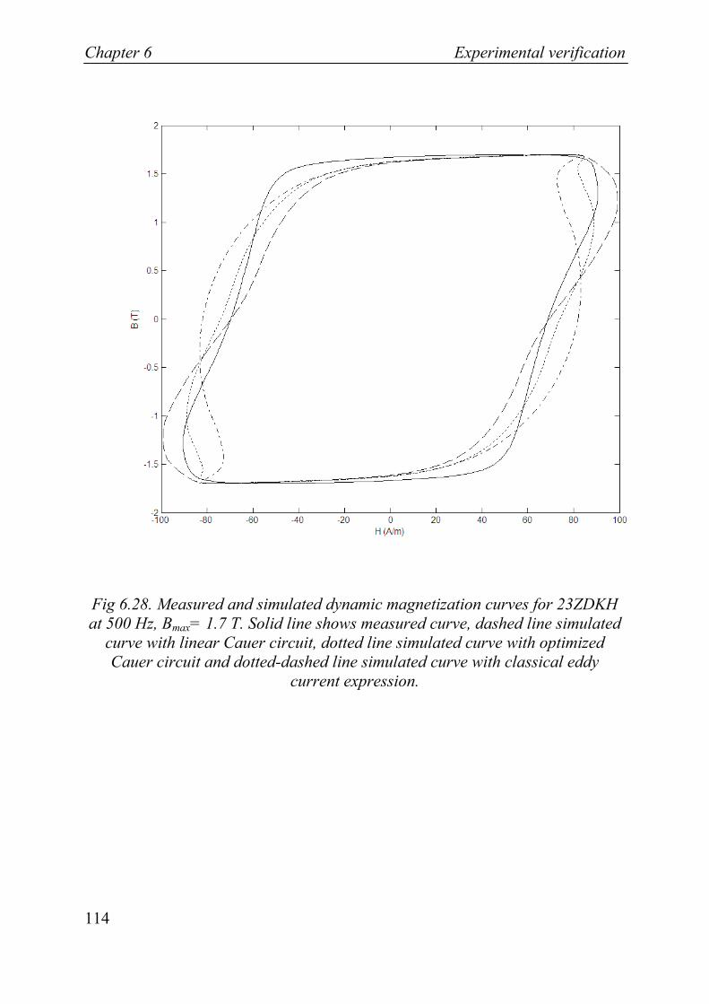
Chapter 6 Experimental verification
114
Fig 6.28. Measured and simulated dynamic magnetization curves for 23ZDKH at 500 Hz, Bmax= 1.7 T. Solid line shows measured curve, dashed line simulated
curve with linear Cauer circuit, dotted line simulated curve with optimized Cauer circuit and dotted-dashed line simulated curve with classical eddy
current expression.

Experimental verification Chapter 6
115
Fig 6.29. Measured and simulated dynamic magnetization curves for 23ZDKH at 2500 Hz, Bmax= 1.7 T. Solid line shows measured curve, dashed line simulated
curve with linear Cauer circuit, dotted line simulated curve with optimized Cauer circuit and dotted-dashed line simulated curve with classical eddy
current expression.
Some examples of simulations at different frequencies with the optimized Cauer circuit are shown for M5 and 23ZDKH in Fig 6.30 and Fig 6.31, respectively. It is seen that the broadening of the curves are replicated in a satisfying way.

Chapter 6 Experimental verification
116
Fig 6.30. Measured (solid) and simulated (dotted) dynamic magnetization curves with optimized Cauer circuit for M5 at Bmax= 0.5 T. Shown frequencies
with increasing width: 50, 500, 1500, 3500 and 5000 Hz.

Experimental verification Chapter 6
117
Fig 6.31. Measured (solid) and simulated (dotted) dynamic magnetization curves with optimized Cauer circuit for 23ZDKH at Bmax= 0.5 T. Shown
frequencies with increasing width: 50, 500, 2500, and 6500 Hz.
As previously mentioned, the value of V0 was adapted for each simulation. Moreover, the values depended on both the amplitude and frequency of B. This is shown in Fig 6.32 - Fig 6.34. It can be seen in Fig 6.32 that V0 increases with the amplitude for a fixed frequency. The increase is nearly linear until the material reaches saturation, where the its value increases faster. The same dependency has earlier been reported by other authors [44].
Furthermore, the results shown in Fig 6.33 and Fig 6.34 show that the value of V0 also increases with the frequency. However, it seems to flatten out at around 1000 Hz. This implies that the formulation of this parameter needs to be modified.

Chapter 6 Experimental verification
118
Fig 6.32. Estimated values of the parameter V0 at 50 Hz for M5 (solid) and M700-50A (dashed) at different amplitudes.
Fig 6.33. Estimated values of the parameter V0 at Bmax = 0.5 T for M5 (solid) and M700-50A(dashed) at different frequencies.

Experimental verification Chapter 6
119
Fig 6.34. Estimated values of the parameter V0 at Bmax = 1.7 T for M5 (solid) and M700-50A(dashed) at different frequencies.
6.1.6.1 Conclusions and discussion It has been shown in the previous sections that the dynamic magnetization model (Cauer circuit) is able to replicate measured curves in a satisfying way. This has been shown for both applied H-fields and B-fields for different electrical steels and for a wide frequency range.
It has also been shown that optimization of the regions in the Cauer circuit improves the results.
Furthermore, it has been shown that the excess loss parameter V0 depends both on the frequency and the amplitude of B. It can also be dependent on the waveform of B.
It should be noticed that the only adapted parameter for dynamic magnetization was V0. It is a great advantage that only one parameter needs to be adapted. This means, that if it is possible to find a frequency-dependency of V0, e.g. for a class of materials, this would yield none parameter to adapt for the dynamic magnetization. However, the parameters of the static model still would be necessary to adapt.
It may be possible to achieve even better fit by adapting the value of V0 individually for each section and/or the sizes of the sections. On the other hand,

Chapter 6 Experimental verification
120
that would make the adapting more complex and there is a trade-off between the simplicity of the model and the correspondence with measurements.
6.1.7 Estimation of the frequency dependence of excess losses One application of the Cauer circuit model is to estimate the frequency dependence of the excess losses. It was seen in the previous section that the excess loss parameter V0 was frequency dependent. However, the formulation of this parameter presumes that the field is homogenously distributed in the material. This is not the case in the considered situations and that could be one reason why V0 did not deep a constant value with increasing frequency. It should be stressed that the values of V0 were estimated. Therefore, if the variations of V0 are due to the inhomogeneous field distribution and not due to frequency dependence of the parameter in itself, still the excess losses could have a square root dependency of frequency.
It was proven by Bertotti that the excess losses had a square root dependency of frequency, however, since he used the classical eddy current expression he could only prove it up to around 300 Hz [19]. On the contrary, with the use of the dynamic magnetization model presented in this thesis it is possible to investigated the excess loss characteristics even at higher frequencies. Therefore, the excess losses of the following materials were investigated:
• M5. Thickness 0.30 mm, width 3.0 cm, grain oriented.
• M700-50A, mixed rolling and transverse directions. Thickness 0.50 mm, width 3.0 cm, nonoriented.
• 23ZDKH. Thickness 0.23 mm, width 3.0 cm, strongly oriented, laser-scribed.
• M330-35A. mixed rolling and transverse directions. Thickness 0.35 mm, width 3.0 cm, nonoriented.
The total losses were measured for these materials according to the description in section 6.1.4. Then, the static hysteresis losses were measured for the

Experimental verification Chapter 6
121
materials. Thereafter, the static and eddy current losses were simulated using optimized Cauer circuits. The difference between the measured total losses and the simulated static plus eddy current losses give the excess losses.
In Fig 6.35 – Fig 6.37 are shown the excess losses for those materials at Bmax = 0.5, 1.1 and 1.7 T, respectively. The excess losses are plotted against the square-root of frequency, in order to facilitate the verification of a square-root dependency. I.e., a linear curve means a square-root dependency. The plots show that at low frequencies, the excess loss increase is faster than linear. However, for Bmax= 0.5 T, when f 1/2 is greater than approximately 15 Hz1/2 the increase is very close to linear for all materials. Furthermore, for Bmax= 1.1 T, there is a close to linear increase for f 1/2 greater than approximately 20 Hz1/2. For Bmax= 1.7 T, the data at higher frequencies are limited, however, the increase seems to be slightly faster than linear. It should be noticed than it the latter case, the materials are run into saturation which could be the reason of the slightly different dependency.
Fig 6.35. Excess losses for different materials at Bmax= 0.5 T plotted against the square-root of frequency. Solid line = M330-35A, dashed-dotted line = M700-
50A, dashed line = M5 and dotted line = 23ZDKH.
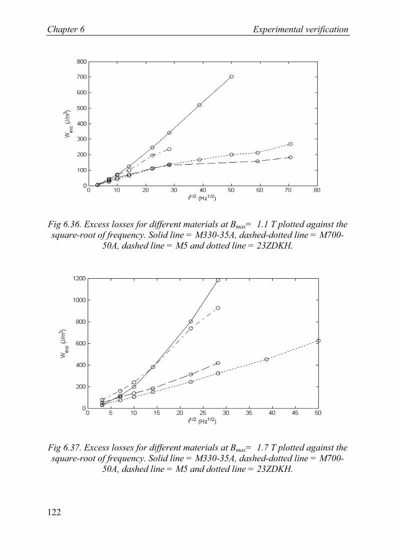
Chapter 6 Experimental verification
122
Fig 6.36. Excess losses for different materials at Bmax= 1.1 T plotted against the square-root of frequency. Solid line = M330-35A, dashed-dotted line = M700-
50A, dashed line = M5 and dotted line = 23ZDKH.
Fig 6.37. Excess losses for different materials at Bmax= 1.7 T plotted against the square-root of frequency. Solid line = M330-35A, dashed-dotted line = M700-
50A, dashed line = M5 and dotted line = 23ZDKH.

Experimental verification Chapter 6
123
6.1.7.1 Discussion It should be stressed that the results in this section strongly depends on the models used. However, it has been shown in section 6.1.6 that the dynamic magnetization model using Cauer circuits is able to replicate measured magnetization curves in a satisfying manner. It has also been shown in section 4.2.1.3 that the inhomogeneous field distribution can be satisfactorily modelled. Therefore, these results are assumed to be correct.
It is interesting that the results indicate that the excess losses have a square-root dependency of the frequency in many cases. This is what Bertotti claimed [19], [30], however, was not able to prove for higher frequencies than approximately 300 Hz.
On the contrary, it seems like the assumption that the parameter V0 is constant with frequency in ref [44] is incorrect. The reason to this incorrectness is that in that study the inhomogeneous field distributions and the saturation effects in the materials are not considered. This fact has also been pointed out by Zirka et al [31].
6.2 Transformer model verification
In order to verify the total transformer model a three-phase three-leg transformer was measured on and simulated. However, only one phase (middle leg) were measured on and simulated. The other terminals were left open during the measurements.
The transformer is at least 20 years old and some of its characteristics are unknown. The nameplate data is 4000 VA apparent power, it is D/Y – connected and the line-to-line voltage ratio is 380 / 750 V. The transformer is shown in Fig 6.38.

Chapter 6 Experimental verification
124
Fig 6.38. Transformer used for measurements.
6.2.1 Measurements In order to verify the model some of the unknown characteristics of the transformer were measured or estimated. These were:
• Number of turns. This was measured using a control winding with 20 turns and applying a voltage to the primary winding and measuring the induced voltages in the control winding and secondary winding. Since the number of turns in the control winding was known, it was possible to calculate the number of turns in the primary and secondary winding. This yielded 420 turns in the primary winding and 500 turns in the secondary winding.
• Resistance of each winding were measured to 1.67 Ω in the primary and 2.25 Ω in the secondary.
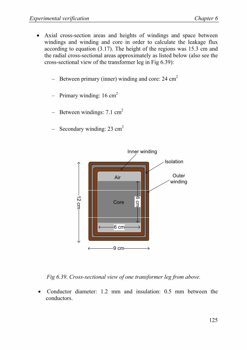
Experimental verification Chapter 6
125
• Axial cross-section areas and heights of windings and space between windings and winding and core in order to calculate the leakage flux according to equation (3.17). The height of the regions was 15.3 cm and the radial cross-sectional areas approximately as listed below (also see the cross-sectional view of the transformer leg in Fig 6.39):
– Between primary (inner) winding and core: 24 cm2
– Primary winding: 16 cm2
– Between windings: 7.1 cm2
– Secondary winding: 23 cm2
Core
Air
Inner winding
Outer winding
Isolation12 cm
9 cm
6 cm
6 cm
Fig 6.39. Cross-sectional view of one transformer leg from above.
• Conductor diameter: 1.2 mm and insulation: 0.5 mm between the conductors.

Chapter 6 Experimental verification
126
• Core cross-section: 6.00 cm x 6.12 cm. Number of laminates in the core: 120. This gave a sheet thickness of 0.50 mm.
• It was not possible to measure the B-H curves of the materials directly. Instead a static major loop was measured on the middle leg (see Fig 6.40). Moreover, this B-H curve includes all effects of the transformer, e.g., losses in joints, leakage flux, air gap losses and magnetostrictive losses due to the bolt holes. There is one bolt hole with a diameter of 15 mm in every joint. As was shown in section 6.1.3.2 magnetic materials are deteriorated by cutting. Furthermore, since the transformer is old the magnetic material can have been subjected to aging [78]. These circumstances together with the fact that the joints are not 45° mitred but 90 ° joints, is probably the main reason that the saturation level is low and the coercivity high. The magnetic flux was measured with a control winding with 20 turns wound around the middle leg and the magnetic field with a Hall probe inserted between the inner winding and the core. The Hall probe cable was very flexible and a sample holder was used to get the probe element perpendicular to the axial direction of the leg. However, the measuring equipment is sensitive to noise, which also can be seen in the figure.
Fig 6.40. Static B-H curve measured on the middle leg of the transformer.

Experimental verification Chapter 6
127
6.2.1.1 Normal operation Measurements were done under normal operation at different frequencies and with different loads on the secondary side. The frequencies were 25, 50 and 250 Hz, respectively and the loads were in the range 1 – 4000 Ω.
The measured quantities were primary and secondary voltages and currents, magnetic field strength and flux density in the core. The voltages and currents were measured using multimeters. Furthermore, the field strength and flux density were measured in the same way as described in the previous section.
The results of the measurements are shown together with the simulated results for the same operation modes in section 6.2.2.1.
6.2.1.2 Non normal operation Measurements of four different non normal operation modes were performed:
• No-load operation.
• Inrush current
• DC-magnetization
• Short-circuit
The results of these measurements are presented in sections 6.2.2.3 - 6.2.2.6.
6.2.2 Simulations A composite transformer model including a core and winding model were used in the simulations of the same operation modes as were measured.
Since the frequency was not higher than 250 Hz, a simplified winding model was used. At these low frequencies the capacitive and eddy current effects in the windings are small [1], [68], [69]. Therefore, those were omitted in the

Chapter 6 Experimental verification
128
simulations. This means that the winding model including capacitive and eddy current effects as presented in Chapter 3 has not been verified. Nevertheless, the leakage flux and resistances of the winding conductors were included in the model.
For modelling of the core it is not enough to lump all the magnetization characteristics into one component. On the contrary, a network of reluctance components has to be used. An example of such a network is shown in Fig 6.41. This type of networks can be made very detailed, however, in order to reduce the simulation time they can optionally be simplified. E.g., the yokes and the leg in one return path have usually the same properties and can therefore be lumped into one component instead of three.
Fig 6.41. Reluctance network for the transformer core with two return paths. The left hysteresis component represents the reluctance in the middle leg. The
two return paths to the right represents the reluctances in each of the other two legs. Moreover, the joints in each return path are represented by the two
shunted hysteresis components. Finally, the air gaps are represented by the linear reluctance component in the middle of the circuit.
In the figure, the joints in each return path are represented by two shunted hysteresis components, since there are two flux paths around the bolt holes in each joint (see Fig 6.42).

Experimental verification Chapter 6
129
φ
φ
Fig 6.42. Flux path in joints. The flux path is divided into two different paths in the core material. This is due to the bolt hole and gives rise to the two shunted
hysteresis components representing the joints in the reluctance network.
In Fig 6.41 the reluctance network has two returns paths, representing the two outer legs of the transformer. However, since in this thesis the transformer is only run in one phase and the two legs have the same characteristics; it is possible to simplify this network. Therefore, the two paths can be represented by one path, with double cross-sectional area in order to yield the same flux density as in the two path case. This simplified network is shown in Fig 6.43.

Chapter 6 Experimental verification
130
Fig 6.43. Simplified reluctance network. Still the left hysteresis component represents the reluctance in the middle leg and the air gap is represented by a
linear reluctance. The two return flux paths have been reduced to one path with double cross-sectional area.
In the hysteresis components in the network shown in Fig 6.43, the core model presented earlier in this thesis was implemented. However, one important task was to determine the parameters of the static hysteresis model. In order to do this the following approach was used:
Since the sheets in the core have a thickness of 0.5 mm they were supposed to be of grade M7, which is a commonly used grade and has this actual thickness. This material is grain oriented and has a magnetization loop similar to and a saturation level almost equal to M5 [85]. The latter material has been used in the core model verification. Therefore, for the static part of the magnetization model the parameters for M5 with an arctan anhysteretic curve were used. However, since the material has probably been aged; the losses are increased and thereby the coercivity is also increased [79], [80]. Therefore, parameters adapted for aging were used in the hysteresis components.
Moreover, the effect of cutting was implemented by adapting the parameters of the static part of the hysteresis components representing the joints. It was shown in section 6.1.3.2 that especially the permeability and saturation level were affected by cutting. It was found that the effect of cutting implemented in the

Experimental verification Chapter 6
131
hysteresis components representing the joints, was highly affecting the B-H curve of the transformer.
The parameters were adapted to fit a simulated static B-H curve to the measured curve, shown in Fig 6.40. The parameter values are shown in Table 6.3 and the corresponding static B-H curves in Fig 6.44. Note that the parameters for M7 governing the saturation regime is a little different from that for M5 presented in section 6.1.2. However, the resulting curve is almost the same, since different sets of parameters can yield similar curves. Also note that since a variable pinning strength is used both t0, y and k0 affect the coercivity. The values of q, c and the number of pseudo particles (25) were given by fitting of simulated minor loops to measured minor loops.
The total air gap was given by adapting the linear reluctance element with respect to the mean slope of the measured and simulated B-H curves in Fig 6.45. This yielded a total air gap length of around 50 micrometers, which seems reasonable. In that figure is shown the resulting B-H curve for the transformer when using the reluctance network with the adapted parameters due to aging and cutting.
Table 6.3. Parameter values for the different hysteresis components.
χ*μ0 Ms* μ0 k0 t0 y b be c q
M7 0.45 1.75 8 2 2.22 240 14 0.02 0
M7 aged 0.45 1.75 35 2 2.22 240 14 0.02 0
M7 aged and cut
0.35 1.65 47 2 1.2 650 14 0.02 0

Chapter 6 Experimental verification
132
Fig 6.44. Plot of static major loops for the different cases. Solid line shows simulated curve of M7, dotted line shows simulated curve of aged M7 whereas
dashed-dotted shows simulated curve of aged and cut M7.
Fig 6.45. Measured static B-H curve of the whole transformer (solid line) compared with simulated curve (dashed line).
Experimental verification Chapter 6
133
6.2.2.1 Normal operation First the measured normal operation modes with different loads were simulated.
One crucial parameter in these simulations is the parameter V0 of the excess loss term in the core model. It was shown in section 6.1.6 that this parameter increases with the amplitude of B. Moreover, it was reported in ref. [44] that this parameter is close to linear in the amplitude range 0.1 - 0.5 T. The values, of V0 as a function of Bmax were fitted at the operation mode with highest amount of core losses, i.e., 4000 Ω load at 25, 50 and 250 Hz, respectively. This gave V0 (Bmax = 0.63) = 0.11 A/m, V0 (Bmax = 0.31) = 0.03 A/m and V0 (Bmax = 0.062) = 0.008 A/m. In addition V0 (Bmax = 0) = 0 was used. The values of V0 at other amplitudes of B were then given through linear interpolation.
Measured and simulated voltages and currents are compared for different loads in Table 6.4 - Table 6.8. In the tables, index p denotes primary winding and index s secondary winding. Also the simulated value of the amplitude of B for each case is shown in the tables. The importance of the core model increases with increasing load resistance and decreasing frequency, since the core losses are high in these cases. Conversely, the importance of the winding model increases with decreasing load resistance and increasing frequency. It can be seen in the tables that for the operations with 30 – 4000 Ω load the simulated results agree very well with the measured, especially for the secondary voltage and primary current. However, it can be seen that at 1 Ω load the simulated and measured results are diverging.

Chapter 6 Experimental verification
134
Table 6.4. Measured and simulated voltages and currents of the primary and secondary winding, respectively. Load on secondary winding is 4000 Ω. Shown values are peak values. The accuracy of the measured currents is ± 2 mA and of
the measured voltages ± 1.6 V.
Frequency (Hz)
Vp (V)
Vs, meas (V)
Vs, sim (V)
Ip, meas (A)
Ip, sim (A)
Is, meas (A)
Is, sim (A)
Bmax (T)
25 146.0 174.4 173.5 0.102 0.102 0.044 0.043 0.63
50 146.0 175.1 173.5 0.084 0.084 0.044 0.043 0.31
250 146.0 175.4 173.6 0.068 0.068 0.046 0.043 0.062
Table 6.5. Measured and simulated voltages and currents of the primary and secondary winding, respectively. Load on secondary winding is 2000 Ω. Shown values are peak values. The accuracy of the measured currents is ± 2 mA and of
the measured voltages ± 1.2 V.
Frequency (Hz)
Vp (V)
Vs, meas (V)
Vs, sim (V)
Ip, meas (A)
Ip, sim (A)
Is, meas (A)
Is, sim (A)
Bmax (T)
25 120.7 143.3 143.3 0.126 0.124 0.071 0.072 0.50
50 121.2 144.0 143.9 0.111 0.114 0.072 0.072 0.26
250 121.4 144.2 144.2 0.095 0.100 0.072 0.072 0.052
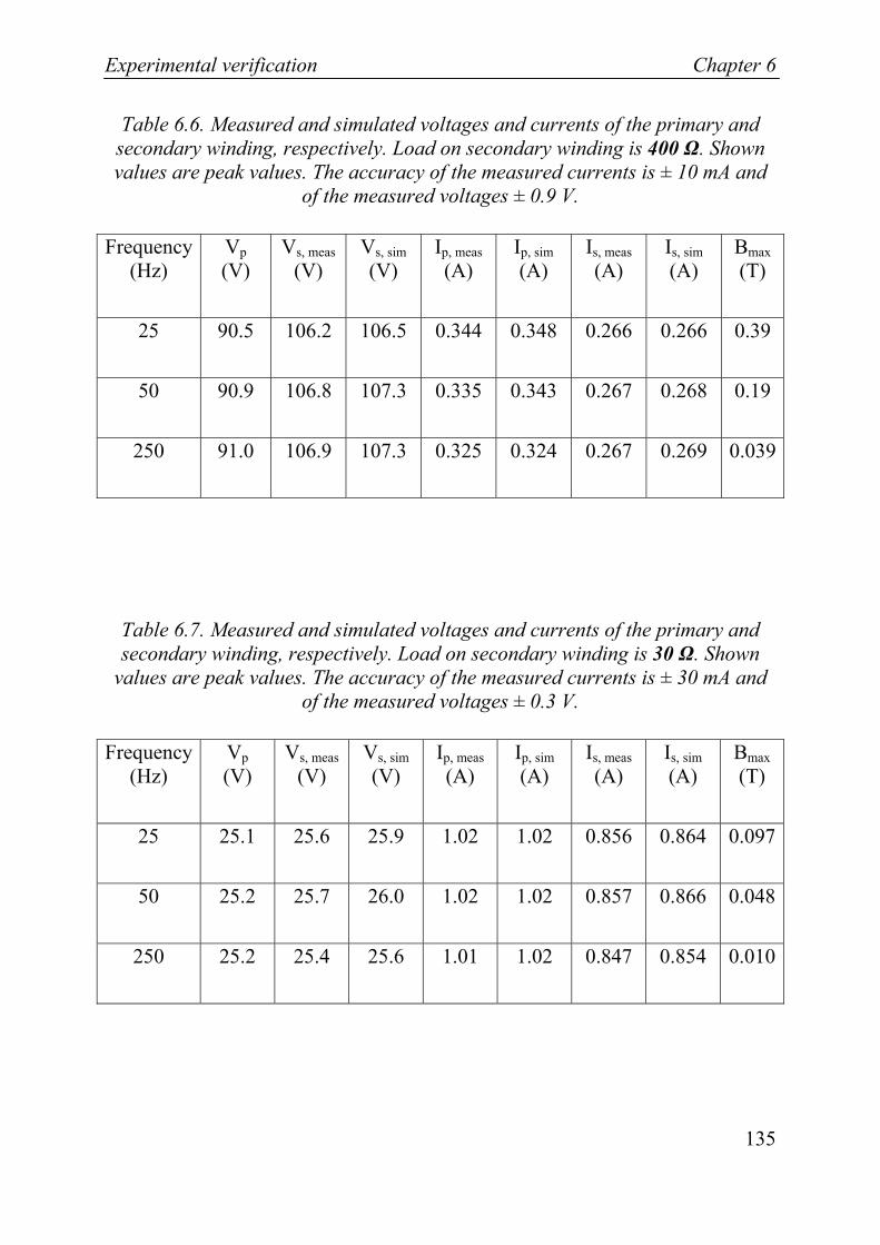
Experimental verification Chapter 6
135
Table 6.6. Measured and simulated voltages and currents of the primary and secondary winding, respectively. Load on secondary winding is 400 Ω. Shown values are peak values. The accuracy of the measured currents is ± 10 mA and
of the measured voltages ± 0.9 V.
Frequency (Hz)
Vp (V)
Vs, meas (V)
Vs, sim (V)
Ip, meas (A)
Ip, sim (A)
Is, meas (A)
Is, sim (A)
Bmax (T)
25 90.5 106.2 106.5 0.344 0.348 0.266 0.266 0.39
50 90.9 106.8 107.3 0.335 0.343 0.267 0.268 0.19
250 91.0 106.9 107.3 0.325 0.324 0.267 0.269 0.039
Table 6.7. Measured and simulated voltages and currents of the primary and secondary winding, respectively. Load on secondary winding is 30 Ω. Shown
values are peak values. The accuracy of the measured currents is ± 30 mA and of the measured voltages ± 0.3 V.
Frequency (Hz)
Vp (V)
Vs, meas (V)
Vs, sim (V)
Ip, meas (A)
Ip, sim (A)
Is, meas (A)
Is, sim (A)
Bmax (T)
25 25.1 25.6 25.9 1.02 1.02 0.856 0.864 0.097
50 25.2 25.7 26.0 1.02 1.02 0.857 0.866 0.048
250 25.2 25.4 25.6 1.01 1.02 0.847 0.854 0.010

Chapter 6 Experimental verification
136
Table 6.8. Measured and simulated voltages and currents of the primary and secondary winding, respectively. Load on secondary winding is 1 Ω. Shown
values are peak values. The accuracies of the measured currents are ± 50 mA at 25 and 50 Hz and ± 30 mA at 250 Hz. The accuracies of the measured primary
and secondary voltages are ± 0.08 V and ± 0.01 V, respectively.
Frequency (Hz)
Vp (V)
Vs,
meas (V)
Vs, sim (V)
Ip, meas (A)
Ip, sim (A)
Is, meas (A)
Is, sim (A)
Bmax (T)
25 8.94 1.78 1.88 2.11 2.24 1.78 1.88 0.02
50 8.98 1.77 1.86 2.08 2.22 1.77 1.86 0.012
250 9.04 1.32 1.33 1.58 1.56 1.34 1.33 0.004
6.2.2.2 Discussion The obtained results indicate that the model with a detailed core model and a simple winding model yields good results when the core losses are dominating. However, when the winding losses and leakage inductance increase the simplified winding model has to be replaced with a more detailed model in order to correctly replicate the measured results. One obvious source of error is the modelling of the leakage flux; since the geometrical values needed to calculate those, were not known exactly. Conversely, they were roughly estimated by visual inspection.
Unfortunately, the time limit of the project was reached before the proposed, more detailed winding model was able to be verified.
6.2.2.3 No-load operation With the secondary side unloaded, the magnetization of the core will easily go into saturation. This will affect the magnetization loop of the core and also the current in the primary winding, i.e., the magnetizing current. The shape of this
Experimental verification Chapter 6
137
current will be non-sinusoidal due to the nonlinearity of the magnetization loop of the material.
No-load currents were measured at the primary side at four different frequencies: 5, 10, 20 and 50 Hz. The 5 and 10 Hz tests were measured with amplitude of 50 and 100 V, respectively, applied to the primary winding. The 25 and 50 Hz tests were measured at the maximum amplifier output voltage, i.e. with amplitude of 146 V.
The same cases were simulated with the transformer model. The results of these simulations are shown in Fig 6.46 - Fig 6.49. It can be seen that at 5 and 10 Hz the simulations are in very good agreement with the measured curves. At 50 Hz the simulations are also in good correspondence with the measurements, however, at 20 Hz the correspondence is slightly lower. The reason to the discrepancy at the latter frequency is not known. It shall be noted that at 50 Hz the amplitude of the applied field is not high enough to bring the material into saturation. In this case the importance of the minor loop model is higher than for the other simulated cases were the major loop model is more important.

Chapter 6 Experimental verification
138
Fig 6.46. Magnetizing current in no-load operation at 5 Hz. Solid line is measured curve and dashed line simulated curve.
Fig 6.47. Magnetizing current in no-load operation at 10 Hz. Solid line is measured curve and dashed line simulated curve.

Experimental verification Chapter 6
139
Fig 6.48. Magnetizing current in no-load operation at 20 Hz. Solid line is measured curve and dashed line simulated curve.
Fig 6.49. Magnetizing current in no-load operation at 50 Hz. Solid line is measured curve and dashed line simulated curve.
Chapter 6 Experimental verification
140
6.2.2.4 Inrush current When switching in a transformer to a net, a phenomenon called inrush current can occur. In normal operation and steady state condition the magnetization loop in the core will be symmetrical around origin. However, if the transformer has been in operation and switched off, there is usually a remanent flux in the core. Therefore, when the transformer is switched in, the core will be magnetized again and due to the remanence the magnetization loop may now not be symmetrical around origin [1], [26].
This phenomenon can occur even without remanence in the core, depending on where in the voltage cycle the transformer is switched in. The time integral of the voltage gives the flux so if the switching occurs in the early part of one of the two half periods of a cycle the flux will reach high values in the end of that half period. Theoretically, the flux can reach maximum twice the normal operation flux plus the remanent flux. Moreover, it may drive the core into saturation which will give a peak current much higher than the current in steady state condition. However, due to the losses in the transformer, the steady state condition is reached after a time. For power frequencies this time is in the range of 10 – 20 seconds for modern transformer [1], [26].
In order to test the transformer model one inrush current situation when the transformer core was put into the remanent state, Br = 0.72 ± 0.008, was measured. The primary current was measured in the following condition:
• f = 50 Hz, secondary side unloaded, VAC, peak = 62.7 ± 0.5 V. Supply swith-on angle = 0 °.
The same situation was then simulated. The primary currents found from the measurements and simulations, respectively are compared in Fig 6.50 - Fig 6.52. It can be seen that the simulated currents are in good correspondence with the measured values.

Experimental verification Chapter 6
141
Fig 6.50. First 100 periods of primary winding current starting from the maximum remanent state. In this case the secondary side is unloaded. The upper
figure shows measured values and the lower picture shows simulated values.

Chapter 6 Experimental verification
142
Fig 6.51. The first ten periods of the primary winding current for the same case as in Fig 6.50. Solid line shows measured current and dashed line simulated
current.
Fig 6.52. The primary winding current after ca 50 periods for the same case as in Fig 6.50 Solid line shows measured current and dashed line simulated
current.
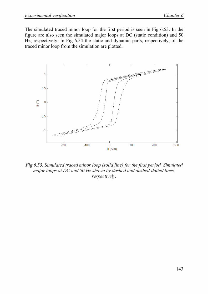
Experimental verification Chapter 6
143
The simulated traced minor loop for the first period is seen in Fig 6.53. In the figure are also seen the simulated major loops at DC (static condition) and 50 Hz, respectively. In Fig 6.54 the static and dynamic parts, respectively, of the traced minor loop from the simulation are plotted.
Fig 6.53. Simulated traced minor loop (solid line) for the first period. Simulated major loops at DC and 50 Hz shown by dashed and dashed-dotted lines,
respectively.

Chapter 6 Experimental verification
144
Fig 6.54. Minor loop contribution. Solid line shows the first traced minor loop and dashed line the static part of that loop. The static major loop (dashed-dotted
line) is shown as comparison.
It can be seen in Fig 6.51 and Fig 6.52 that the negative peak values of the measured curves is decreasing faster than the corresponding simulated curve values. It should be stressed that in this situation the magnetization is tracing minor loops as seen in Fig 6.53 and Fig 6.54. Moreover, the latter figure shows that the static part of the minor loops gives the major contribution to the losses of the dynamic minor loops when the material is close to saturation. In the showed example this is the case in the initial stage and is due to the fact that the rate of change is small there. Therefore, it is essential that the static minor loop model is correct.
Therefore, in order to improve the dynamic magnetization model for inrush currents, the static minor loop model should be improved
6.2.2.5 DC-magnetization There can be situations when a small DC-voltage or -current is added to the AC-voltage of one or both windings of the transformer. This DC-component can be due to non-balanced operation of DC-converters connected to the transformer or geomagnetically induced currents [1]. This DC-component will give an offset in the magnetization of the core and also to the currents in the windings. Furthermore, it can drive the core up into saturation and thereby increase the current dramatically.

Experimental verification Chapter 6
145
Two measurements with DC-magnetization were performed:
• VAC, peak = 10 ± 0.08 V, VDC = 0.3 ± 0.001 V, f = 50 Hz, load = 100 ohm
• VAC, peak = 25 ± 0.3 V, VDC = 0.3 ± 0.001 V, f = 50 Hz, load = 400 ohm
Before the DC-offsets were applied the transformer was demagnetized. Then the primary current was measured and the same situations were simulated. Comparisons between the measurements and simulation are seen in Fig 6.55 and Fig 6.56. It can be seen in the figures that the simulated currents are in good correspondence with the measurements. It shall be noted that the mean value of the flux density was ca 0.95 T in both situations. Comparing this with the magnetization loop of the transformer core, seen in Fig 6.40, it can be understand that some parts of the core were in saturation. Thereby, it is essential that the model replicates the real object correctly. One reason to the small discrepancies between the simulated and measured results can be due to the fact that the characteristics of the measured object are not known exactly. Another reason can be that the model is not replicating the object perfectly due to the imperfections in the minor loop model as was the case for the inrush currents.

Chapter 6 Experimental verification
146
Fig 6.55. Current in primary winding for the 100 ohm load case. Solid line shows measured current and dashed line simulated current.
Fig 6.56. Current in primary winding for the 400 ohm load case. Solid line shows measured current and dashed line simulated current.

Experimental verification Chapter 6
147
6.2.2.6 Short-circuit Under short-circuit condition at 50 Hz the measured voltage was 11.7 ± 0.2 V (rms). Measured and simulated short-circuit current were 3.51 ± 0.08 A and 3.46 A, respectively.
6.2.3 Discussion Most of the characteristics and parameters of the measured object, necessary for the model were unknown. This fact complicated the modelling process, since it required estimation and adaption of several parameters. Furthermore, it was found, when building the model, that the magnetic core of the transformer was highly degraded due to cutting and most likely also due to aging. This fact also complicated the modelling attempt, since the material parameters could not be obtained from measurements in e.g. an Epstein frame. Nevertheless, with use of a reluctance network for the core, with parameter adapted for aging and cutting of material, it was possible to achieve good correspondence between the measurements and simulations.
The best correspondence was achieved in conditions when the core losses were dominant, i.e., no-load, low load, inrush current and DC-magnetization. On the contrary, under the conditions when the winding losses, i.e., high load, were dominant, the correspondence was slightly lower. Therefore, the core model is considered to be satisfactory, even if the minor loop model can be improved further. However, the winding model should be improved. Nonetheless, with respect to the complexity of the measured object, the transformer model is considered to yield satisfactorily results.
An advantage with the proposed transformer model is the use of the detailed dynamic magnetization core model. In the core model verification section it was shown that this model yields correct results up into at least the kHz range. At low frequencies the static model is the most important, however, at higher frequencies the dynamic model becomes essential.
It is also interesting that it was possible to use a test object, with most of the parameters unknown and also highly degraded and, thereafter, build a model of that object that in high extent replicated the characteristics of the object.


Conclusions and future work Chapter 7
149
Chapter 7
Conclusions and future work
7.1 Conclusions
In this thesis, a time-domain transformer model including loss phenomena in both the core and the windings has been presented. The model includes core phenomena as magnetic static hysteresis, eddy currents and excess losses. Moreover, the model includes winding phenomena as eddy currents, capacitive effects and leakage flux.
For modelling of the core losses, Bergqvist´s lag model has been used for the static magnetization part. Some modifications of this model, e.g. regarding the anhysteretic curve, have been proposed. This model has been shown to yield good correspondence with measurements, especially for major loops.
A dynamic magnetization model using Cauer circuits for modelling of eddy currents and Bertotti´s statistical loss model for excess losses has been assessed. One benefit with the Cauer circuit model is that it automatically includes the inhomogeneous field distribution due to eddy currents. Another benefit is that for adapting the simulated curves to measured curves it is only needed to fit one parameter, V0, in the excess loss term in addition to the static magnetization model. The dynamic model has been verified to yield good agreement with measurements both for controlled sinusoidal H-fields and B-fields up to several kHz for electrical steels. Moreover, it has been shown that it is possible to investigate the inhomogeneous field distribution due to eddy current shielding in magnetic materials using this model.
Chapter 7 Conclusions and future work
150
Furthermore, the frequency dependence of excess losses has been studied using this model. The results indicate that the excess losses have a close to square-root dependency of frequency. Moreover, the statistical loss theory [19] implies that the parameter V0 should be constant with the frequency; however, it has been shown in this thesis that that is not the case for electrical steels. One reason for this can be that the field distribution is varying with the frequency and since the value of V0 is dependent on the peak magnetization, it will be affected by the field distribution.
A winding model including an analytical expression for the skin effect and proximity effect in the winding conductors has been used. Furthermore, the capacitive effects and leakage flux has been included in the model. This model has an upper theoretical frequency limit at 100 kHz.
Moreover, a composite three-phase transformer model containing the proposed core and winding models has been used. The frequency limit of this model is the same as for the winding model.
The composite one-phase transformer model containing the proposed core model and a simplified winding model has been verified through measurements on a real transformer. This has shown that the model shows good agreement with measurements in no-load conditions and in low load conditions up to 250 Hz. Furthermore, it has shown good correspondence with measurements in non-normal operation conditions like inrush current and DC-magnetization.
7.2 Future work
• The proposed winding model should be verified and its validity with respect to frequency and model parameter settings investigated.
• In the core model the static hysteresis model should be improved, especially regarding the modelling of minor loops. E.g., the distribution function of the pseudo particles and the relation between reversible and irreversible processes should be studied more in detail.

Conclusions and future work Chapter 7
151
• In the dynamic magnetization model the optimization of the Cauer circuit sections and the frequency and amplitude dependency of the parameter V0 could be studied. If it is possible to find that dependency for a class of material, this would make this model a very useful tool. Then the only necessary adapting step would be to fit the static curve to the measured static curve.
• The composite transformer model should also be validated in other operation modes like transient overvoltage.
• A more detailed reluctance network model of the transformer including three dimensional flux paths in the tank and construction details should be developed and verified.
• A static magnetization model that takes B as input and returns H should be developed.

Appendix
153
Appendix I Derivation of analytical expression for eddy currents
Here follows the derivation of the analytical expression of eddy currents as it is presented in ref. [20].
When all the elements are in steady-state condition, the quasi-static form of Ampère’s law can be written as:
∇× =H J (8.1)
We also have
σ=J E (8.2)
Since the fields in the coil vary sinusoidal we get the following relations in complex notation:
( ) ( )jˆRe tt e ω=H H (8.3)
( ) ( )jˆRe tt e ω=J J (8.4)
( ) ( )jˆRe tt e ω=E E (8.5)
( ) ( )jˆRe tt e ω=B B (8.6)
Where “^” denotes a complex amplitude and Re the real part of a complex number.

Appendix
154
Introducing the complex conjugate, denoted with “*”, in equation (8.1) and multiplying with E we get:
( )ˆ ˆ ˆ ˆ∗ ∗∇× =E H E Ji i (8.7)
Expanding the left term of this equation gives:
( ) ( ) ( )* *ˆ ˆ ˆ ˆ ˆ ˆ∗∇× = −∇ × + ∇×E H E H H Ei i i (8.8)
Faraday’s law written in complex form states:
ˆ ˆjω∇× = −E B (8.9)
Combining equations(8.7), (8.8) and (8.9) now yields:
( )* *ˆ ˆ ˆ ˆ ˆ ˆjω∗−∇ × = −E H E J H Bi i i (8.10)
Using equations (8.2), μ=B H , and the complex pointing vector
*1ˆ ˆ ˆ2
= ×P E H (8.11)
in equation (8.10) yields:
*1ˆ ˆ ˆ ˆ ˆ2 jωμσ
∗− ∇ = −P J J H Hi i i (8.12)
Suppose that the network exist inside a volume V enclosed by a surface S. Then we can integrate over V to get the total power inside the network, referring to Fig 3.2. However, Gauss theorem yields:

Appendix
155
ˆ ˆ ˆV S
dV dS∇ =∫ ∫P P ni i (8.13)
where n is a unit vector normal to S at each point. Assume that all power flow is confined to the cross sections of the input terminals. Then the complex power input is *
t tˆ ˆV I . Now the normal component of the Poynting vector can be written
in terms of the complex power input [83], [84] as:
*t t
ˆ ˆ ˆˆS
dS V I− =∫ P ni (8.14)
where tV and tI are the complex amplitudes of the voltage and current applied to the network through S. This yields:
* *t t
*
1 1ˆ ˆ ˆ ˆ ˆ ˆ ˆj2
1 ˆ ˆ ˆ ˆj2 2
V V
V V
V I dV dV
dV dV
ωμσ
ωμσ
∗
∗
⎞⎛= − ∇ = − =⎜ ⎟⎝ ⎠
= −
∫ ∫
∫ ∫
P J J H H
J J H H
i i i
i i (8.15)
Now the complex impedance Z at the terminal is
t
t
ˆ( j ) j ˆ
VZ R XI
ω = + = (8.16)
Expanding the right term of equation (8.16) by *tI gives
*
t t*
t t
ˆ ˆˆ ˆ
V IZI I
= (8.17)
Using equation (8.15) in equation (8.17) and changing the notation of the current from It to I gives
Appendix
156
** *
1 ˆ ˆ ˆ ˆ( j ) jˆˆ ˆˆ2 2V V
Z dV dVII II
ωμωσ
∗= −∫ ∫J J H Hi i (8.18)
Realizing that 2*ˆˆ ˆII I= finally yields
*2 2
1 ˆ ˆ ˆ ˆ( j ) jˆ ˆ2 2V V
Z dV dVI I
ωμωσ
∗= −∫ ∫J J H Hi i (8.19)
This equation is equal to equation (3.1).
Now we want to find J and H inside the coil. Start with the magnetic diffusion equation:
2 ddt
μσ∇ =BB (8.20)
In complex form the magnetic diffusion equation is:
2 ˆ ˆjωμσ∇ =B B (8.21)
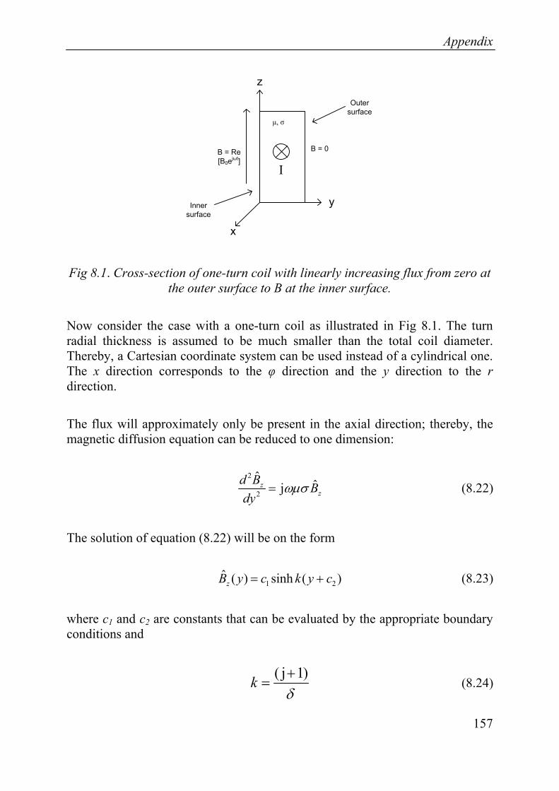
Appendix
157
I
y
x
z
B = 0B = Re [B0ejωt]
μ, σ
Outer surface
Inner surface
Fig 8.1. Cross-section of one-turn coil with linearly increasing flux from zero at the outer surface to B at the inner surface.
Now consider the case with a one-turn coil as illustrated in Fig 8.1. The turn radial thickness is assumed to be much smaller than the total coil diameter. Thereby, a Cartesian coordinate system can be used instead of a cylindrical one. The x direction corresponds to the φ direction and the y direction to the r direction.
The flux will approximately only be present in the axial direction; thereby, the magnetic diffusion equation can be reduced to one dimension:
2
2
ˆ ˆjzz
d B Bdy
ωμσ= (8.22)
The solution of equation (8.22) will be on the form
1 2ˆ ( ) sinh ( )zB y c k y c= + (8.23)
where c1 and c2 are constants that can be evaluated by the appropriate boundary conditions and
( j 1)kδ+
= (8.24)
Appendix
158
where δ is the skin-depth defined as:
2δ
ωμσ= (8.25)
According to Ampère’s law and the ampere-turn diagram the boundary conditions are:
0
ˆ ( ) 0
ˆ ( 0)
z
z
B y dIB y
lμ
= =
= = (8.26)
Here I is the current in the turn, l the axial length of the coil and d is the thickness of the turn.
The boundary condition at y = d gives:
1 2ˆ ( ) sinh ( ) 0zB y d c k d c= = + = (8.27)
The nontrivial solution of this equation is:
2c d=− (8.28)
Next, the boundary condition at y = 0 gives:
01
ˆ ( 0) sinh ( ) sinhzIB y c k d kd
lμ
= = − = − = (8.29)
This gives the constant c1 as:
01 sinh
Icl kdμ
= − (8.30)
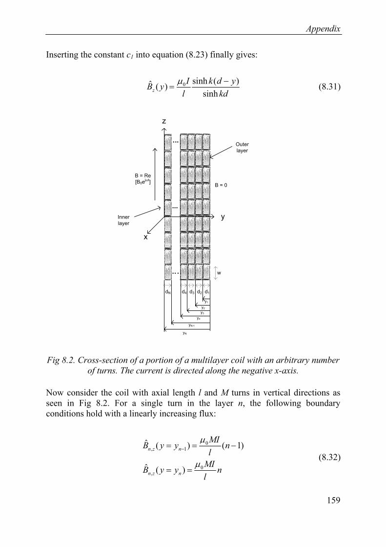
Appendix
159
Inserting the constant c1 into equation (8.23) finally gives:
0 sinh ( )ˆ ( )sinhz
I k d yB yl kdμ −
= (8.31)
y
x
z
B = 0
B = Re [B0ejωt]
Outer layer
Inner layer
w
dN d4 d3 d2 d1
yN
yN-1
y4
y3
y2
y1
Fig 8.2. Cross-section of a portion of a multilayer coil with an arbitrary number of turns. The current is directed along the negative x-axis.
Now consider the coil with axial length l and M turns in vertical directions as seen in Fig 8.2. For a single turn in the layer n, the following boundary conditions hold with a linearly increasing flux:
0, 1
0,
ˆ ( ) ( 1)
ˆ ( )
n z n
n z n
MIB y y nl
MIB y y nl
μ
μ
−= = −
= = (8.32)

Appendix
160
where M is the number of turns in every layer, I is the current in each turn and l the axial length of the coil. In the same way as for the single turn case, the flux density is found from the new boundary conditions.
This yields with d = yn - yn-1 :
0 1 0,
1
0 1 1
1
sinh ( )ˆ ( ) ( 1)sinh ( )
sinh ( ) ( 1)sinh ( )sinh ( )
n nn z
n n
n n n n
n n
MI k y y y MIB y nl k y y lMI k y y y n k y yl k y y
μ μ
μ
−
−
− −
−
− −= + − =
−
− − + − −=
−
(8.33)
This numerator can be expanded to contain y in both the terms. However, this requires lengthy calculations and will not be shown here. The final expression will then be:
( ) ( )( ) ( ) ( )( )( )( )
10,
1
ˆ sinh 1 sinhˆsinh
n nn z
n n
n k y y n k y yMIB yl k y y
μ −
−
⎡ ⎤− − − −= ⎢ ⎥
−⎢ ⎥⎣ ⎦(8.34)
From Fig 8.2 we realize that
lwM
= (8.35)
and by using the relation between field and flux density in free space we can express the field in layer n as:
( ) ( )( ) ( ) ( )( )( )( )
1,
1
ˆ sinh 1 sinhˆsinh
n nn z
n n
n k y y n k y yIH yw k y y
−
−
⎡ ⎤− − − −= ⎢ ⎥
−⎢ ⎥⎣ ⎦ (8.36)
According to Ampère’s law:
∇× =H J (8.37)

Appendix
161
The magnetic field has only a component in the z direction which results in that the current density only has a x component given by:
ˆ ( )ˆ ( ) z
xdH yJ y
dy= (8.38)
Using this expression with equation (8.36) gives:
( ) ( )( ) ( ) ( )( )( )( )
1,
1
ˆ cosh 1 coshˆsinh
n nn x
n n
n k y y n k y ykIJ yw k y y
−
−
⎡ ⎤− − − −= ⎢ ⎥
−⎢ ⎥⎣ ⎦ (8.39)
Now it is possible to use equations (8.36) and (8.39) in equation (8.19) and calculate the corresponding impedance in a turn with circumference ln in the n´th layer by the following integration:
( ) ( ) ( ) ( )1 1
2 2ˆ ˆ ˆ ˆj
ˆ ˆ2 2
n n
n n
y yn n
n x x z zy y
l w l wZ J y J y dy H y H y dyI I
ωμ
σ − −
∗ ∗= −∫ ∫ (8.40)
Carrying out this integration yields the result in equation (3.7).

Appendix
162
Appendix II Determination of parameter values in Bergqvist’s lag model
Here follows a method to determine the parameter values in Bergqvist’s lag model from measured curves.
Start with the mean pinning strength k. The value of this parameter can be found from the total loss of a static major loop in one dimensional excitation. This loss corresponds to the area of all individual pseudo particles. The area of the j:th pseudo particle with pinning λjk is 4Msλjk. If the loss is Psat, the following relation holds:
sat S 04 ( )P M k dλς λ λ
∞= ∫ (9.1)
Now k can be found through the normalization condition:
( ) 1dλς λ λ =∫ (9.2)
For anisotropic materials this procedure has to be repeated in the orthogonal directions.
The total magnetization including reversible parts is expressed as:
[ ]( )an an λ0
( ) ( )c M P dς λ λ∞
= +∫ kM M H H (9.3)
Thereby, the normalization condition is changed to:
Appendix
163
0
( ) 1d cς λ λ∞
= −∫ (9.4)
Moreover, the density function ς(λ) which gives the weight of the pseudo particles can e.g. be a Gaussian distribution:
2( )( ) e p qA λς λ − −= (9.5)
This expression contains three unknown parameters A, p and q, governing the distribution. However, this can be reduced to one through the aforementioned normalization conditions.
Inserting equation (9.5) into the second normalization condition, equation (9.4) gives:
( )( )1 erf 12Ac qp
π+ + = (9.6)
Here, erf (q) is the so called error function, defined as:
2
0
2erf ( ) eq
yq dyπ
−≡ ∫ (9.7)
Inserting equation (9.5) into the first normalization condition in equation (9.2)gives:
( )( )( )2
2 1 erf e 12
qA q qp
π −+ + = (9.8)
This has yielded two equations for the four unknown parameters c, q, p and A. Therefore, two additional parameters are needed. These can be found e.g. from measurements of a virgin curve. At small magnetization levels the virgin curve has a parabolic form, approximately (here we suppose that the material is isotropic, so the vector notation is changed to scalar):

Appendix
164
20 0( ) (0) (0)M H H Hχ κ= + (9.9)
Where χ0(0) and κ0(0) are the Rayleigh parameters found from the measurements of the virgin curve. These parameters can be used to give the additional two equations using the following method:
In the initial condition H = 0, the magnetization history is wiped out and Pλk[H] = 0 for all λ. Then when increasing H monotonically the following play operator is obtained:
λk
if [ ]
0 if H k H k
P HH k
λ λλ
⎧ − >⎪⎪=⎨⎪ <⎪⎩ (9.10)
Inserting this into equation (9.3) the model gives a virgin curve as:
( )/
an an0
( ) ( )H k
M cM H M H k dλ ς λ λ= + −∫ (9.11)
Supposing that H is small and linearizing Man around H = 0 yields:
( )/
an an0
(0) (0)H k
M cM H M H k dλ ς λ′ ′≈ + −∫ (9.12)
Which gives:
2an an
1(0) (0) (0)2
M c H Hk
χ ς χ≈ + (9.13)
Here
an an(0) (0)Mχ ′= (9.14)
Appendix
165
Using equation (9.13) with equation (9.4) yields:
2 2
an an(0) e (0)2
qAM c H Hk
χ χ−≈ + (9.15)
To get correspondence between the model and experiments we have to choose:
0
an
(0)(0)
c χχ
= (9.16)
and:
2
0 01(0) (0) (0) e (0)
2 2qA
k kκ ς χ χ−= = (9.17)
Notice that this method also requires that the anhysteretic curve is known. Now, we have four equations for the four parameters q, c, p and A, i.e. equations (9.6), (9.8), (9.16) and (9.17). This equation system can not be solved analytically, however, it can be simplified, with the following procedure:
The parameter c is trivially given through equation (9.16). The parameter p is given from equation (9.6) as:
( )( )1 erf
21
A qp
c
π +=
− (9.18)
Setting in this expression into equation (9.8) yields:
( )( )( )
( )( )( )22
2
2 11 1 erf e
1 erfqc
q qA q
ππ
−−= + +
+ (9.19)
Moreover, the parameter A is given from equation (9.17) as:
Appendix
166
2
0
2 (0)e(0)
qkA κχ
= (9.20)
Finally, inserting this expression for A and the expression for c into equation (9.19) gives:
( )( )
( )( )( )2
2
2
00
an2
(0)1 (0)e(0)
1 1 erf e(0) 1 erf
q
qq qk q
χ χχ
πκ π
−
−
⎛ ⎞⎟⎜ ⎟−⎜ ⎟⎜ ⎟⎜⎝ ⎠= + +
+ (9.21)
The only unknown parameter is now q. To find the value of q the equation has to be solved numerically.

Appendix
167
Appendix III Determination of the pseudo particle distribution function from measurements
In the proposed modification to Bergqvist’s lag model with a modified play operator, it is possible to determine the pseudo particle distribution from measured major loop and anhysteretic curve. The governing equation is:
( )an0
( )M M H k dς λ λ∞
± =∫ ∓ (10.1)
Now write this integral as a discrete sum with a set of discrete, equidistance field values hi, spanning the whole range of the major loop:
an( ) ( ) ( )i i j jj
M h hM h h hς± = Δ∑ ∓ (10.2)
Let us consider the positive branch of the major loop, M+. Then equation (10.2) can be solved for the distribution ς(hj) by numerical inversion of the matrix:
( ) ( )ij an i j jm hM h h hςΔ= − (10.3)

Appendix
168
Appendix IV Performance of dynamic measurement with controlled H-field
Hall probe
A Hall probe uses two electrodes with an electrical conducting, non-ferrous material in between. Between the electrodes a current, with current density J, is forced to pass. When inserting the probe into a magnetic field, the charge carriers experience a force according to Lorentz’s law:
0V
dVμ= ×∫∫∫F J H
This force creates a displacement of the charge carriers in the orthogonal direction to J and H, and thereby an electric field in that direction. Two electrodes are positioned in this direction and the electric field gives a voltage, U, between these electrodes. F, E and U are related through the following expressions:
Q=F E (10.4)
l
U = ∫ iE dl (10.5)
Here l is the length between the electrodes which the voltage is measured over. Furthermore, Q is the total charge of the charge carriers with total force F. If J and V are known, it is thereby possible to calculate H. This is done in a gaussmeter connected to the Hall probe.
One problem with this technique is that the charge carriers scatter into empty places in the atoms in the material. This will of course affect the induced voltage of the electrodes. Therefore, to achieve high accuracy, a long Hall probe should be used.
Appendix
169
In the measurements with the SST it was not possible to use a long Hall probe due to the limits of the SST:s dimensions. Instead a thin Hall probe that measures the field perpendicular to the probe plane, i.e. transverse, was used. It is then important that the plane of the probe is perpendicular to the applied field. Therefore, a holder was used for the probe to align it in the correct direction.
The probe had a low signal to noise ratio and a sensitivity of 10 A/m. Therefore, the B - and H - values were measured for at least 200 periods for every measurement. Thereafter, the mean value for every (H, B) – point of one magnetizing loop was calculated. These mean values were then used for plotting of the hysteresis loops.
Sampling frequency
When running dynamic measurements the ADC:s and DAC:s sampling frequencies become important, since a too low sampling frequency can introduce aliasing effects
The sampling frequency depends on the computer program that governs the output signals of the computer and reads the input signals. The highest sampling frequency that was achieved in the program was 59 kHz, which corresponds to a sampling interval of 17 μs. The sampling frequency is 29 times the measured frequencies so the Nyquist theorem (which states that the sampling frequency must be at least two times the measured frequency to be able to recreate the analog signal correctly [60]) is fulfilled.
Compensation for time lag
It was found that the output from the gaussmeter had a time delay. The reason for this is that the corrected analog output of the gaussmeter is re-created with a DAC from the sampled ADC data from the Hall probe. This raw data is scaled and corrected for several types of error such as frequency response and linearity for both the probe and gaussmeter. This processing takes time and then the data is sent to the DAC for the analog output to create the corrected waveform, which again takes time. Furthermore, the time delay increases with the frequency [82].

Appendix
170
In order to compensate for this time delay, a setup was created for measurement of the time lag between the fluxmeter and gaussmeter. A coil was placed on the surface of a magnetic sheet in the middle of the SST and connected to the fluxmeter. Then, the Hall probe was placed as close as possible to the coil and connected to the gaussmeter. Thereby, both the fluxmeter and the gaussmeter measured the field in the air and the time lag was found by comparing the signals. The following time lags for different frequencies of the applied field were found:
• 1 Hz: no measurable time lag
• 50 Hz: 10 μs
• 500 Hz: 22 μs
• 1 kHz: 37 μs
• 2 kHz: 44 μs
Then, in order to achieve the correct values during B - H curve measurements, the time lags were subtracted from the signal from the gaussmeter. This yielded synchronized signals for both the flux and field.

References
171
References [1] Å. Carlsson, Power Transformer Design Fundamentals, ABB
Transformers, Ludvika, 2000
[2] J. A. Martinez, B. A. Mork, “Transformer modelling for low- and mid-frequency transients – a review”, IEEE Transactions on Power Delivery, Vol. 20, No. 2, p 1625-1632, Apr. 2005
[3] A. Narang, R. H. Brierley, “Topology based magnetic model for steady-state and transient studies for three-phase core type transformers”, IEEE Transactions on Power Systems, Vol. 9, No. 3, pp 1337-1349, Aug. 1994
[4] B. A. Mork, “Five-legged wound-core transformer model: derivation, parameters, implementation, and evaluation”, IEEE Transactions on Power Delivery, Vol. 14, No. 4, p 1519-1526, Oct. 1999
[5] U. D. Annakkage, P. G. McLaren, E. Dirks., R. P. Jayasinghe, A. D. Parker, “A current transformer model based on the Jiles-Atherton theory of ferromagnetic hysteresis”, IEEE Transactions on Power Delivery, Vol. 15, No. 1, pp 57-61, Jan. 2000
[6] D. Dolinar, J. Pihler, B. Grcar, “Dynamic model of a three-phase power transformer”, IEEE Transactions on Power Delivery, Vol. 8, No. 4, p 1811 - 1818, Oct. 1993
[7] E. Dallago, G. Sassone, G. Venchi, “High-frequency power transformer model for circuit simulation”, IEEE Transactions on Power Delivery, Vol. 12, No. 4, p 664-670, Jul. 1997
[8] E. J. Tarasiewicz, A. S. Morched, A. Narang, E. P. Dick, “Frequency dependent eddy current models for nonlinear iron cores”, IEEE Transactions on Power Systems, Vol. 8, No. 2, pp 588-597, May 1993
[9] W. E. Archer, M. F. Deveney, R. L. Nagel, “Nonlinear transformer modeling and simulation”, Proceedings of the 37th Midwest Symposium on Circuits and Systems, pp 665-669, 1994.

References
172
[10] X. S. Chen, P. Neudorfer, “Digital modeling of modern single-phase distribution transformers”, International Conference on Advances in Power System Control, Operation and Management, 1991. APSCOM-91., Vol. 2 pp 914-920,
[11] W. Chandrasena, P. G. McLaren, U. D. Annakkage, R. P. Jayasinghe, E. Dirks, ”Simulation of eddy current effect in transformers”, Proceedings of the 2000 IEEE Canadian Conference, pp. 122 – 126
[12] W. Chandrasena, P. G. McLaren, U. D. Annakkage, R. P. Jayasinghe, ”An improved low-frequency transformer model for use in GIC studies”, IEEE Transactions on Power Delivery, Vol. 19, No. 2, p 643-651, Apr. 2004
[13] F. de Leon, A. Semlyen, “Complete transformer model for electromagnetic transients”, IEEE Transactions on Power Delivery, Vol. 9, No. 1, p 231-239, Jul. 1997
[14] F. de Leon, A. Semlyen, “Time domain modelling of eddy current effects for transformer transients”, IEEE Transactions on Power Delivery, Vol. 8, No. 1, p 271-280, Jan. 1993
[15] F. de Leon, A. Semlyen, “Efficient calculation of elementary parameters of transformers”, IEEE Transactions on Power Delivery, Vol. 7, No. 1, pp 376-383, Jan. 1992
[16] F. de Leon, A. Semlyen, “Reduced order model for transformer transients”, IEEE Transactions on Power Delivery, Vol. 7, No. 1, pp 361-369, Jan. 1992
[17] F. de Leon, A. Semlyen, “Eddy current add-on for frequency dependent representation of winding losses in transformer models used in computing electromagnetic transients”, IEE Proceedings: Generation, Transmission and Distribution, Vol. 141, No. 3, pp 209-214, May 1994
[18] F. de Leon, A. Semlyen, “Detailed modeling of eddy current effects for transformer transients”, IEEE Transactions on Power Delivery, Vol. 9, No. 2, pp 1143-1150, Apr. 1994

References
173
[19] G. Bertotti, Hysteresis in Magnetism, Academic Press, San Diego, 1998
[20] M. P. Perry, Low frequency electromagnetic design, Marcel Dekker, New York, 1985
[21] M. P. Perry, “Multiple layer series connected winding design for minimum losses”, IEEE Transactions on Power Apparatus and Systems, Vol. PAS-98, No. 1, Jan/Feb 1979
[22] M. P. Perry, “Multiple layer parallel connected air-core inductor design”, IEEE Transactions on Power Apparatus and Systems, Vol. PAS-98, No. 4, July/Aug 1979
[23] A. Bergqvist, On Magnetic Hysteresis Modeling, Ph. D. thesis, KTH, Stockholm. 1994
[24] A. Bergqvist, “A phenomenological differential-relation-based vector hysteresis model”, Journal of Applied Physics, Vol. 75, No 10, p 5484-5486, May 1994
[25] A. Bergqvist, “Magnetic vector hysteresis model with dry friction-like pinning”, Physica B: Condensed Matter, Vol. 233, No. 4, p 342-347, Jun. 1997
[26] J. J. Winders, Power Transformers: Principles and Applications, Marcel Dekker Inc., New York, 2002
[27] V. Korenivski, J. C. Slonczewski, Introduction to Spintronics, KTH, Stockholm, 2009
[28] P. Holmberg, Modelling the Transient Response of Windings, Laminated Steel Cores and Electromagnetic Power Devices by Means of Lumped Circuits, Ph. D. thesis, Uppsala University, Uppsala, 2000
[29] D. C. Jiles, Introduction to Magnetism and Magnetic Materials, Chapman and Hall, London, 1991
References
174
[30] G. Bertotti, “General Properties of Power Losses in Soft Ferromagnetic Materials”, IEEE Transactions on Magnetics, Vol. 24, No. 1, pp 621-630, Jan. 1988
[31] A. Broddefalk, M. Lindenmo, “Dependence of the power losses of a non-oriented 3% Si-steel on frequency and gauge”, Journal of Magnetism and Magnetic Materials, 304 (2006), e586-588
[32] S. E. Zirka, Y. I. Moroz, P. Marketos. A. J. Moses, “Evolution of the loss component in ferromagnetic laminations with induction level and frequency”, Journal of Magnetism and Magnetic Materials, 320 (2008), e1039-e1043
[33] S. E. Zirka, Y. I. Moroz, P. Marketos. A. J. Moses, “Viscosity-Based Magnetodynamic Model of Soft Magnetic Materials”, IEEE Transactions on Magnetics, Vol. 42, No. 9, pp 2121-2132, Sept. 2006
[34] S. E. Zirka, Y. I. Moroz, P. Marketos. A. J. Moses, “Dynamic hysteresis modelling”, Physica B, Vol. 343, No. 1-4, pp. 90-95, 2004
[35] S. E. Zirka, Y. I. Moroz, P. Marketos, A. J. Moses, D. C. Jiles, T. Matsuo, “Generalization of the classical method for calculating dynamic hysteresis loops in grain-oriented electrical steels”, IEEE Transactions on Magnetics, Vol. 44, No. 9, pp 2113-2125, Sept. 2008
[36] S. E. Zirka, Y. I. Moroz, P. Marketos. A. J. Moses, “Novel approach to modelling losses in electrical steel laminations”, The Fourth International Conference on Computation in Electromagnetics, 2002. CEM 2002.
[37] D. C. Jiles, D. L. Atherton, “Theory of magnetic hysteresis”, Journal of Magnetism and Magnetic Materials, Vol. 61, p 48-60, 1986
[38] D. C. Jiles, “A Self Consistent Generalized Model for the Calculation of Minor Loop Excursions in the Theory of Hysteresis”, IEEE Transactions on Magnetics, Vol. 28, No. 5, pp 2602-2604, Sept. 1992

References
175
[39] F. Preisach, Über die magnetische Nachwirkung”, Zeitschrift f94, pp 277-302, 1935,
[40] I. D. Mayergoyz, Mathematical Models of Hysteresis, Springer-Verlag, New York, 1991
[41] A. Ivanyi et al, Preisach Memorial Book, Akadémiai Kiadó, Budapest, 2005
[42] J. Krah, Modeling of losses in power transformers from dc to the low kilohertz range, Ph. D. thesis, KTH, Stockholm, 2005
[43] J. H. Krah, A. J. Bergqvist, “Numerical optimization of a hysteresis model”, Physica B: Condensed Matter, Vol. 343 pp 35-38, 2005
[44] E. Barbisio, F. Fiorillo, C. Cagusa, “Predicting Loss in Magnetic Steels Under Arbitrary Induction Waveform and With Minor Hysteresis Loops”, IEEE Transactions on Magnetics, Vol. 40, No. 4, p 1810-1819, Jul. 2004
[45] F. Fiorillo, A. Novikov, “Power Losses Under Sinusoidal, Trapezodial and Distorted Induction Waveform”, IEEE Transactions on Magnetics, Vol. 26, No. 5, p 2259-2561, Sep. 1990
[46] D.C. Jiles, “Modelling the Effects of Eddy Current Losses on Frequency Dependent Hysteresis in Electrically Conducting Media”, IEEE Transactions on Magnetics, Vol. 30, No. 6, p 4326-4328, Nov. 1994
[47] A. Schoppa, H. Louis, F. Pude, Ch. von Rad, “Influence of abrasive waterjet cutting on the magnetic properties of non-oriented electrical steel”, Journal of Magnetism and Magnetic Materials, Vol. 254-255, p 370-372, Jan. 2003
[48] W. Cauer, “Die Verwirklichung von Wechselstromwiderstanden vorgeschriebener Frequenzabhagigkeit (The realization of alternating-current resistances of a prescribed frequency)”, Archiv für Elektrotechnik und Machinenbau, Vol 17, No 4, p 355-388, 1926

References
176
[49] D. L. Atherton, M. Schönbächler, “Measurements of Reversible Magnetization Component”, IEEE Transactions on Magnetics, Vol. 24, No. 1, pp 616-620,Jan. 1988
[50] J. A. Szpunar, D. L. Atherton, B. Szpunar, “Analysis of the Irreversible Processes of Magnetization in Steel”, IEEE Transactions on Magnetics, Vol. 23, No. 1, pp 300-303, Jan. 1987
[51] P. Holmberg, A. Bergqvist, G. Engdahl, “Modelling eddy currents and hysteresis in a transformer laminate”, IEEE Transactions on Magnetics, Vol. 33, No. 2, pp 1306-1309, Mar. 1997
[52] P. Holmberg, A. Bergqvist, G. Engdahl, “Modelling a Magnetomechanical Drive by a Coupled Magnetic, Electrical and Mechanical Limped Circuit Approach”, Journal of Applied Physics, Vol. 81, pp. 4091-4093, Apr. 1997
[53] R. Herzog, S. Vullioud, R. Amstad, G. Gorka, P. Muellhaupt, R. Longchamp, “Self-Sensing of Non-Laminated Axial Magnetic Bearings: Modelling and Validation”, Journal of System Design and Dynamics, Vol. 3, No. 4, 2009, pp. 443-452
[54] A. Davoudi, P. L. Chapman, J. Jatskevich, A. Khaligh, “Reduced-Order Modeling of High-Fidelity Magnetic Equvivalent Circuits”, IEEE Transactions on Power Electronics, Vol. 24, No. 12, Dec. 2009
[55] E. Hallén, Electromagnetic Theory, London, 1962
[56] M. Langevin, Ann. De Chem. et. Phys. 5, 1905
[57] G. Engdahl, private communication
[58] D. Bormann, private communication
[59] J. Buck, “Automatic Hysteresisgraph Speeds Accurate Analysis of Soft Magnetic Materials”, PCIM, Feb 2000

References
177
[60] Nyquist H., "Certain topics in telegraph transmission theory," Trans. AIEE, vol. 47, p 617-644, Apr. 1928
[61] A.J. Moses, N. Derebasi, G. Loisos, A. Schoppa, “Aspects of the cut-edge effect stress on the power loss and flux density distribution in electrical steel sheets”, Journal of Magnetism and Magnetic Materials, Vol. 215-216, p 690-692, Jun. 2000
[62] T. Nakata, M. Nakano, K. Kawahara, “Effects of stress due to cutting on magnetic characteristics of silicon steel“ IEEE Translation Journal on Magnetics in Japan, Vol. 7, No. 6, p 453-457, Jun. 1992
[63] P. Carlberg, The cutting of electrical steel sheet, Surahammars bruk, Surahammar, 1971
[64] D. C. Jiles, D. L. Atherton, “Ferromagnetic hysteresis” IEEE Transactions on Magnetics, Vol. 19, No. 5, pp 2183-2185, Sep. 1983
[65] P. L. Dowell, “Effects of eddy currents in transformer windings”, Proc. Inst. Elect. Eng., Vol. 113, pp 1387-1394, Aug. 1966
[66] J. A. Ferreira, “Improved analytical modeling of conductive losses in magnetic components”, IEEE Transactions on Power Electronics, Vol. 9, No. 1, pp 127-131, Jan. 1994
[67] A. M. Urling, V. A. Niemela, G. R. Skutt, T. G. Wilson, “Characterizing high-frequency effects in transformer windings – a guide to several significant articles”, Fourth Annual IEEE Applied Power Electronics Conference and Exposition, 1989. APEC' 89. Conference Proceedings 1989
[68] A. Reatti, M. K. Kazimierczuk, “Comparison of various methods for calculating the AC resistance of inductors”, IEEE Transactions on Magnetics, Vol. 38, No. 3, pp 1512-1518, May 2002
[69] H. Tavakoli, A high frequency transformer winding model for FRA applications”, Lic. thesis, KTH , Stockholm, 2009

References
178
[70] Y. Shibuya, S. Fujita, “High frequency model and transient response of transformer windings”, IEEE/PES Transmission and Distribution Conference and Exhibition 2002: Asia Pacific, Vol. 3, pp 1839-1844, 2002
[71] A. De, N. Chatterjee, “Part winding resonance: demerit of interleaved high-voltage transformer winding”, IEE Proceedings - Electric Power Applications, Vol. 147, No. 3, pp 167-174, May 2000
[72] X. Nan, C. R. Sullivan, “An improved calculation of proximity-effect loss in high-frequency windings of round conductors”, IEEE 34th Annual Power Electronics Specialist Conference, 2003. PESC '03. Vol. 2, pp 853-860, 2003
[73] J. G. Zhu, S. Y. R. Hui, V. S. Ramsden, “Discrete modelling of magnetic cores including hysteresis eddy currents and anomalous losses” IEE Proceedings A : Science, Measurement and Technology, Vol. 140, No. 4, pp 317-320, 1993
[74] J. G. Zhu, S. Y. R. Hui, V. S. Ramsden, ”A generalized dynamic circuit model of magnetic cores for low- and high-frequency applications - Part I: Theoretical calculation of the equivalent core loss resistance”, IEEE Transactions on Power Electronics, Vol. 11, No. 2, pp. 246-250, Mar 1996
[75] S. Y. R. Hui, J. G. Zhu, V. S. Ramsden, ”A generalized dynamic circuit model of magnetic cores for low- and high-frequency applications - Part II: Circuit model formulation and implementation”, IEEE Transactions on Power Electronics, Vol. 11, No. 2, pp. 251-259, Mar 1996
[76] J. G. Zhu, S. Y. R. Hui, V. S. Ramsden, ” A dynamic equivalent circuit model for solid magnetic cores for high switching frequency operation”, IEEE Transactions on Power Electronics, Vol. 10, No. 6, pp. 791-795, Nov. 1995
[77] P. R. Wilson, J. N. Ross, A. D. Brown, “Modeling frequency-dependent losses in ferrite cores”, IEEE Transactions on Magnetics, Vol. 40, No. 3, pp 1537-1541, May 2004
References
179
[78] A. J. Moses, “Electrical steels: past, present and future developments”, IEE Proceedings, Vol 137, Pt. A, pp. 233-345, No. 5 Sept 1990
[79] M. F. de Campos, M. Emura, F. J. G. Landgraf, “Consequences of magnetic aging for iron losses in electrical steels”, Journal of Magnetism and Magnetic Materials, Vol. 304 No. 2, pp. e593-e595, September 2006
[80] K. M. Marra, F. J. G Landgraf, V. T. Buono, “Magnetic losses evolution of a semi-processed steel during forced aging treatments” Journal of Magnetism and Magnetic Materials, Vol. 320, No. 20, pp. e631-e634, October 2008
[81] IEC 60404-2, Magnetic materials – Part 2: Methods of measurement of the magnetic properties of electrical steel strip and sheet by means of an Epstein frame
[82] Private communication with Mark Green, Sypris Test & Measurement
[83] J. D. Jackson, Classical Electrodynamics, Wiley, New York, 1998
[84] R. M. Fano, L. J. Chu and R.B. Adler, Electromagnetic Fields, Energy, and Forces, Wiley, New York, 1960
[85] Electrical Steel Grain Oriented, Unisil, Unisil-H, ASTM Grades, Cogent Power Ltd
[86] J. Krah, private communication


List of symbols
181
List of Symbols
Symbol Quantity SI-Unit a Langevin function parameter A/m A area m2 A density function parameter B magnetic flux density, magnetic induction T b slope parameter m/H be slope parameter c degree of reversibility C capacitance F d thickness m E electric field strength V/m f frequency Hz G magnetic domain structure parameter H magnetic field strength A/m I electric current A J current density A/m2
k complex wave number rad/m k mean pinning strength Am2/s k0 constant pinning strength Am2/s l magnetic path length m L inductance H M magnetization A/m m magnetization of a pseudo particle A/m Man anhysteretic magnetization A/m Ms saturation magnetization A/m N number of turns in a winding n layer number in a winding np number of pseudo particles n0 phenomenological parameter P power W Pλk play operator q density function parameter R electric resistance Ω t time s
List of symbols
182
Symbol Quantity SI-Unit t0 threshold value Am2/s U voltage V V volume m3 V0 phenomenological parameter A/m W energy J/m3 w width m y slope parameter s/m3
Z impedance Ω Px […] Play-operator with size of play: x Px, c […] Play-operator with size of play: x and degree of reversibility: c S surface area m2 α modified Langevin function parameter β geometric factor for eddy currents δ skin-depth m ε electro motive force V φ magnetic flux Wb γ degree of penetration λ pseudo particle number κ Rayleigh parameter m/A ς density function μ permeability H/m μ´ differential permeability H/m μ0 permeability in free space H/m μr relative permeability σ electical conductivity S/m ℜ reluctance A/Vs χ susceptibility χan (H) susceptibility of anhysteretic curve χ´ differential susceptibility ω angular frequency rad/s θ magneto motive force A η back field A/m
List of acronyms
183
List of acronyms AC Alternating current ADC Analog to digital converter DAC Digital to analog converter DC Direct current EMF Electro motive force FDM Frequency dependent method FEM Finite element method LM Linear method MMF Magneto motive force RMS Root-mean square SST Single sheet tester