NASA Contractor Report 189067

//

_'J;3/

Electromagnetic Finite ElementsBased on a Four-Potential

Variational Principle

James Schuler and Carlos A. Felippa

University of Colorado

Boulder, Colorado

(NASA-CR-189067) ELECTROMAGNETIC FINITE

ELEPhaNTS SASED ON A FOUR-POTENTIAL

VARIATIONAL PRINCIPLE Final Report, Sep.

1989 (Colorado Univ.) 37 p CSCL

November 1991

20K

C,3/39

NgZ-14392

Unclas

0057131

Prepared for

Lewis Research Center

Under Grant NAG3-934

National Aeronautics and

Space Administration

https://ntrs.nasa.gov/search.jsp?R=19920005174 2018-08-30T01:53:47+00:00Z

ELECTROMAGNETIC FINITE ELEMENTS BASED ON

A FOUR-POTENTIAL VARIATIONAL PRINCIPLE

JAMES SCHULER

CARLOS A. FELIPPA

Department of Aerospace Engineering Sciences

and Center for Space Structures and Controls

University of Colorado

Boulder, Colorado 80309-0,_P9, USA

S_RY

We derive electromagnetic finiteelements based on a variationalprinciplethat uses the electro-

magnetic four-potentialas primary variable.This choice isused to construct elements suitablefor

downstrea_n coupling with mechanical and thermal finiteelements forthe analysisofelectromago

netic/mechanical systems that involvesuperconductors. The key advantages of the four-potential

are: the number of degrees of freedom per node remain modest as the problem dimensional-

ity increases,jump discontinuitieson interfacesare naturally _ccomodated, and staticas well

as dynamics axe included without any a prI'oriapproximations. The new elements are tested

on an axisymmetrlc problem under steady-stateforcingconditions. The resultsare in excellent

agreement with analyticalsolutions.

1. INTRODUCTION

The present work is part of a research program for the numerical simulation of electro-

magnetic/mechanical systems that involve superconductors. The simulation involves the

interaction of the following four components:

(1) Mechanical Fields: displacements, stresses, strains and mechanical forces.

(2) Thermal Fields: temperature and heat fluxes.

(3) Electromagnetic (EM) Fields: electric and magnetic field strengths and fluxes, cur-

rents and charges.

(4) Coupling Fields: the foundamental coupling effect is the constitutive behavior of

the materials involved. Particularly important are the metallurgical phase change

phenomena triggered by thermal, mechanical and EM fields.

1.I Finite Element Treatment

The first three fields (mechanical, thermal and electromagnetic) are treated by the finite

element method. This treatment produces the spatial discretization of the continuum into

mechanical, thermal and electromagnetic meshes of finite number of degrees of freedom.

The finite element discretization may be developed in two ways:

(I) Simultaneous Treatment. The whole problem is treated as an indivisible whole. The

three meshes noted above become tightly coupled, with common nodes and elements.

(2) Staged Treatment. The mechanical, thermal and electromagnetic components of the

problem are treated separately. Finite element meshes for these components may

be developed separately. Coupling effectsare viewed as information that has to be

transferred between these three meshes.

The present research follows the staged treatment. More specifically,we develop finite

element models /or the fields in isolation, and then treat coupling effects as interaction

forces between these models. This "divide and conquer" strategy is ingrained in the parti-

tioned treatment of coupled problems [4,16], which offers significant advantages in terms of

computational efficiency and software modularity. Another advantage relates to the way

research into complex problems can be made more productive. It centers on the obser-

vation that some aspects of the problem are either better understood or less physically

relevant than others. These aspects may be then temporarily left alone while efforts are

concentrated on the less developed and/or more physically important aspects. The staged

treatment is better suited to this approach.

1.2 Mechanical Elements

Mechanical elements for this research have been derived using general variational principles

that decouple the element boundary from the interior thus providing efficient ways to work

2

out coupling with non-mechanical fields. The point of departure was previous research into

the free-formulation variational principles reported in Ref. [5]. A more general formulation

for the mechanical elements, which includes the assumed natural strain formulation, was

established and reported in Refs. [5,6,14,15]. New representations of thermal fields have

not been addressed as standard formulations are considered adequate for the coupled-field

phases of this research.

2. ELECTROMAGNETIC ELEMENTS

The development of electromagnetic (EM) finite elements has not received to date the

same degree of attentiom given to mechanical and "thermal elements. Part of the reason

is the widespread use of analytical and semianalytical methods in electrical engineering.

These methods have been highly refined for specialized but important problems such as

circuits and waveguidu. Thus the advantages of finite elements in terms of generality have

not been enough to counterweight established techniques. Much of the EM finite element

work to date has been clone in England and k well described in the surveys by Davies [1]

and Trowbridge [21]. The general impression conveyed by these surveys is one of an un-

settled subject, reminiscent of the early period (1960-1970) of finite elements in structural

mechanics. A great number of formulations that combine flux, intensity, and scalar po-

tentials are described with the recommended choice varying according to the application,

medium involved (polarizable, dielectric, semiconductors, etc.) number of space dimen-

sions, time-dependent characteristics (static, quasi-static, harmonic or transient) as well

as other factors of lesser importance. The possibility of a general variational formulation

has not apparently been recognized.

In the present work, the derivation of electromagnetic (EM) elements is based on a vari-

ational formulation that uses the four-potential as primary variable. The electric field is

represented by a scalar potential and the magnetic field by a vector potential. The for-

mulation of these variational principle proceeds along lines previously developed for the

acoustic fluid problem [7,8].

The main advantages of using potentials as primary variables as opposed to the more

conventional EM finite elements based on intensity and/or flux fields are, in order or

importance:

1. Interface discontinuities are automatically taken care of without any special interven-

tion.

2. No approximations are invoked a priori since the general Maxwell equations are used.

3. The number of degrees of freedom per finite element node is kept modest as the

problem dimensionality increases.

4. Coupling with the mechanical and thermal fields, which involves derived fields, can

be naturally evaluated at the Gauss points at which derivatives of the potentials are

evaluated.

Following a recapitulation of the basic field equations, the variational principle is stated.3

The discretization of these principle into finite element equations produces semidiscrete

dynamical equations, which are specialized to the axisymmetric case. These equations are

validated in a simulation of a cylindrical conductor wire.

3. ELECTROMAGNETIC FIELD EQUATIONS

8.1 The Mazwell Equation.s

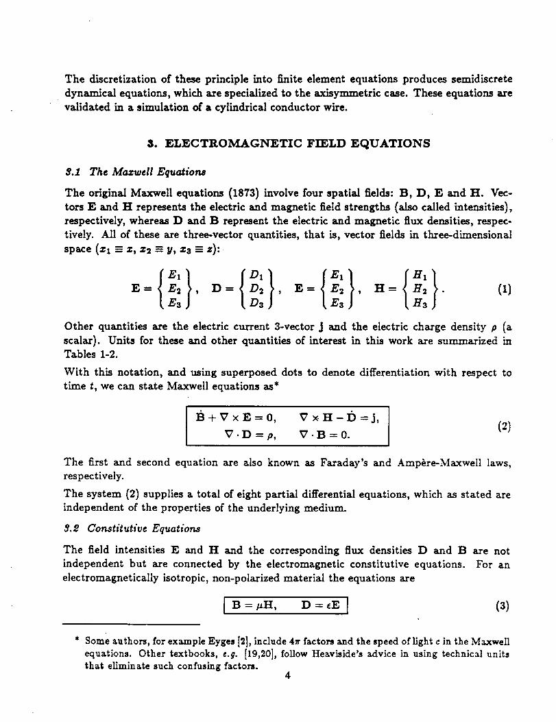
The original Maxwell equations (1873) involve four spatial fields: B, D, E and H. Vec-

tors E and H represents the electric and magnetic field strengths (also called intensities),

respectively, whereas D and B represent the electric and magnetic flux densities, respec-

tively. All of these are three-vector quantities, that is, vector fields in three-dimensional

space (zl - z, z2 - y, z3 --- z):

{ol}E= E2 , D= D2 , E= E2 , H= H2 •

E3 D3 Ea Ha

(1)

Other quantities are the electric current 3-vector j and the electric charge density p (a

scalar). Units for these and other quantities of interest in this work are summarized in

Tables 1-2.

With this notation, and using superposed dots to denote differentiation with respect to

time t, we can state Maxwell equations as*

]3+VxE=O,

V.D=p,

The first and second equation axe also known as Faxaday's and Ampere-Maxwell laws,

respectively.

The system (2) supplies a total of eight partial differential equations, which as stated are

independent of the properties of the underlying medium.

;_.P. Constitutive Equations

The field intensities E and H and the corresponding flux densities D and B are not

independent but axe connected by the electromagnetic constitutive equations. For an

electromagnetically isotropic, non-polarized material the equations axe

[ B=.uH, D=eE I (3)

* Some authors,forexample Eyges [2],include4r factorsand the speed oflightc in the Maxwell

equations. Other textbooks, e.g.[19,20],followHeaviside'sadvice in using technicalunits

that eliminatesuch confusing factors.4

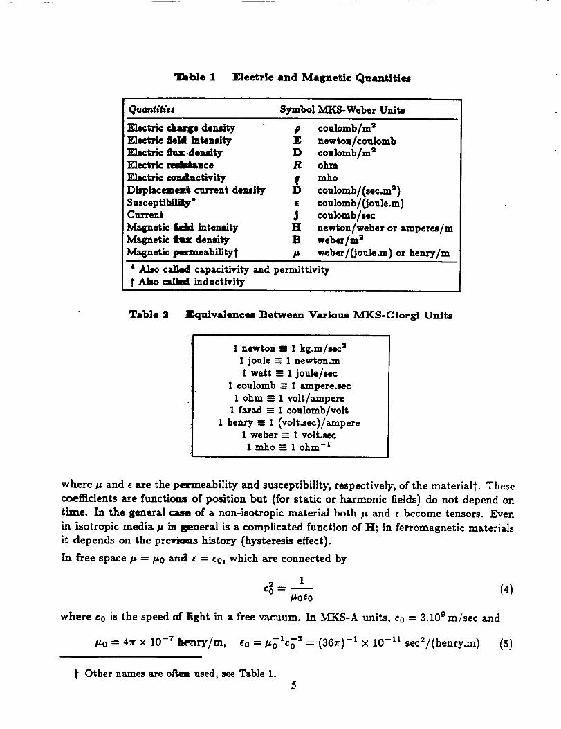
3Bable 1 FJectrtc and Magnetic Quantities

Quantitiel Symbol lvfKS-Weber Units

Electric chrome density

Electric field intensity

Electric flu densityE]ectr]c reaimka=ce

Electric condt_ctivity

Dkplacemes_ current density

Susceptlbs3i_"Current

Magnetic fidd Intensity

M_petic aix density

lV_gnetic pmrmeabiliCyt

p coulomb/m =

E newton/coulombD coulomb/m 2R ohm

f mho

D coulomb/(secan 2)

coulomb/0ouh.m )

j coulomb/Nc

H newton/weber or aanperes/m

B weber/m 2

/z weber/0oulean ) or hem'y/m

* Also callat capacitivity and permittivity

t Also called inductivity

Table 2 ]_quivl]enees Between Various I_4:KS-Glorgi Unite

1 newton -- 1 kg.m/sec 2

1 joule -- 1 newton.m

1 watt -- 1 joule/sec

1 coulomb --" 1 ampereJec

1 ohm -= 1 volt/ampere

1 farad -- 1 coulomb/volt

1 henry --" 1 (volt._ec)/ampere1 weber -- 1 volt.sec

lmho-- 1 ohm -L

where # and • are the permeability and susceptibility, respectively, of the materialt. These

coefficients are functions of position but (for static or harmonic fields) do not depend on

time. In the general case of a non-isotropic material both # and e become tensors. Even

in isotropic media # in Ileneral is a complicated function of H; in ferromagnetic materials

it depends on the previems history (hysteresis effect).

In free space/, = #o and • = co, which are connected by

/_o•o

where co is the speed of Hght in a free vacuum. In MKS-A units, co = 3.10 ° m/sec and

#o = 4_r x 10 -T henry/m, EO -- _O1CO 2 -- (36") -1 X 10 -11 sec2/(henry.m) (5)

t Other names are oftem used, see Table 1.

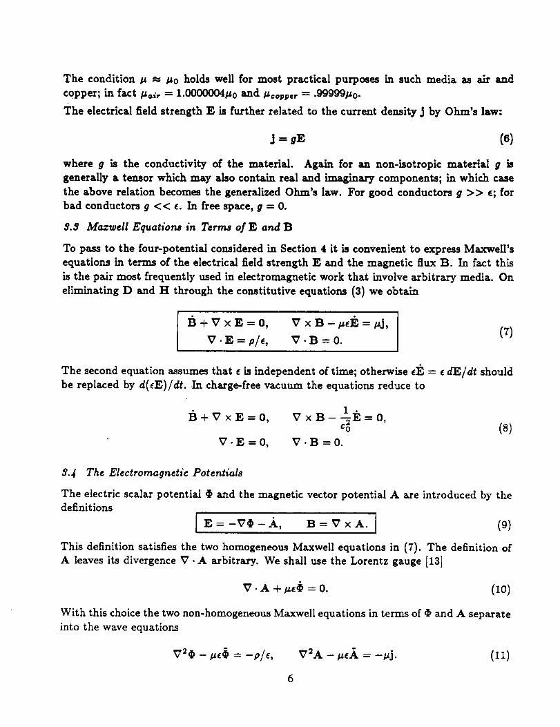
The condition # _ #o holds well for most practical purposes in such media as air and

copper; in fact/_=i, = 1.0000004#o and/_cop_=, = .99999#o.

The electrical field strength E is further related to the current density j by Ohm's law:

j = (6)

where g is the conductivity of the material. Again for an non-isotropic material g k

generally a tensor which may also contain real and imaginary components; in which case

the above relation becomes the generalized Ohm's law. For good conductors g >> e; for

bad conductors g << e. In free space, g = O.

$.$ Mazwell Equation_ in Terms of E and B

To pass to the four-potential considered in Section 4 it is convenient to express MaxwelI's

equations in terms of the electrical field strength E and the magnetic flux B. In fact this

is the pair most frequently used in electromagnetic work that involve arbitrary media. On

eliminating D and H through the constitutive equations (3) we obtain

B+VxE=O,

V .E = pl_,

V x B - #_, = #j,

V.B=0.(7)

The second equation assumes that e is independent of time; otherwise _]_ = c dE/dt should

be replaced by d(_E)/dt. In charge-free vacuum the equations reduce to

VXB-co 2 =0,

V.B-0.

(s)

&.4 The Electromagnetic Potentials

The electricscalar potential (_and the magnetic vector potential A axe introduced by the

definitions

[ E=-V_)-A, B=VxA. (9)

This definition satisfies the two homogeneous Maxwell equations in (7). The definition of

A leaves its divergence V. A arbitrary. We shall use the Lorentz gauge [13]

V.A+#E_=0. (10)

With this choice the two non-homogeneous Maxwell equations in terms of (Dand A separate

into the wave equations

V2¢, - #_ = -p/e, V2A - _X = -#j. (11)

6

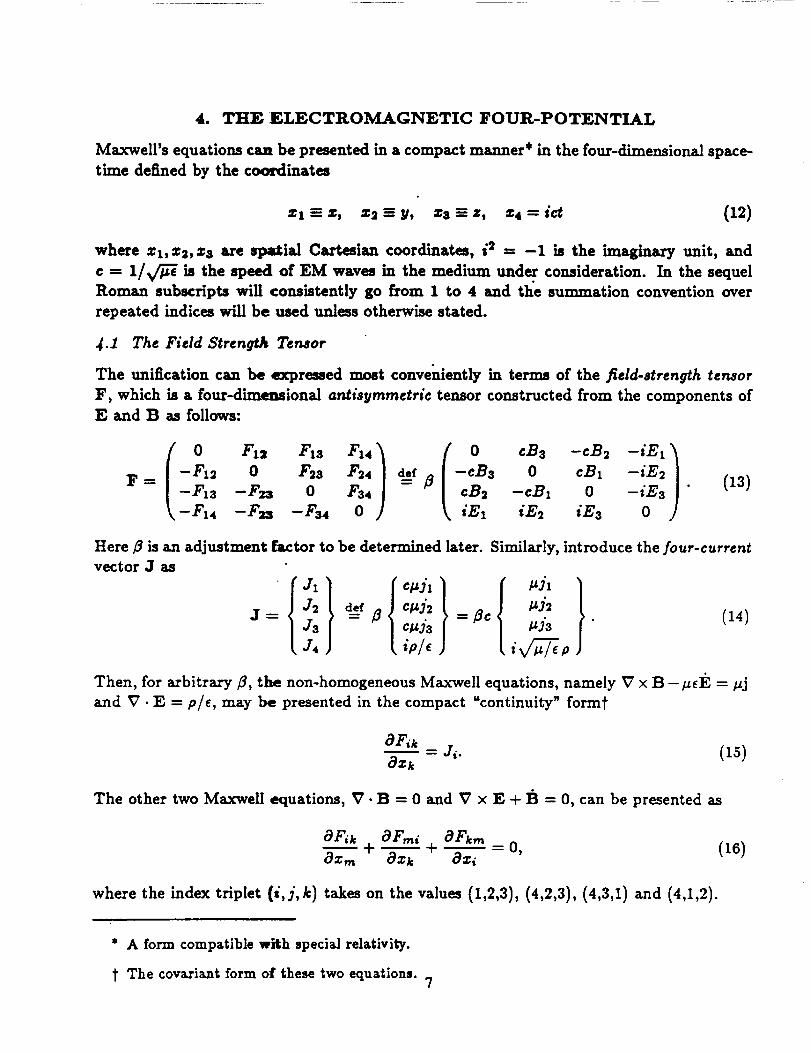
4. THE ELECTROMAGNETIC FOUR-POTENTIAL

Maxwell's equations can be presented in a compact manner* in the four-dimensional space-

time defined by the coordinates

zl=z, z2=y, za=z, z4=ict (12)

where zx, za, za are spatiM Cartesian coordinates, i _ = -I is the imaginary unit, and

e = I/v/_ is the speed of EM waves in the medium under consideration. In the sequel

Roman subscripts will consistently go from 1 to 4 and tlxe summation convention over

repeated indices will be used unless otherwise stated.

4.1 The Field Stren_h Tensor

The unification can be expressed most conveniently in terms of the field-strength terror

F, which is a four-dimemion_l antisyrnrnetri¢ tensor constructed from the components of

E and B as follows:

-F12 0 F2s F24 d.f -cBs 0 cBx -iE2 (13)F = -Fls -Fz3 0 Fs4 = /_ cBa -¢B1 0 -iEs "

-Fx4 -F_ -Fs4 0 iEx iE2 iEs 0

Here _ isan adjustment fm:tor to be determined later.Similarly,introduce the/our-current

vector J as

j 32 de__f_ cl_j2 = _c _J2 (14)Ja c js M3 "

J4 ip/( i l,

Then, for arbitrary 8, the non-homogeneous Maxwell equations, namely V x B -/_E]_ = #j

and V • E = p/_, may be presented in the compact "continuity" forint

aF k0%-[= J'" (is)

The other two Maxwell equations, V. B = 0 and V x E + ]3 = 0, can be presented a.s

OF k OFm OFkm--+--+--=0,Ox._ Ozj, Oxi

(16)

where the index triplet (i,j,k) takes on the values (1,2,3), (4,2,3), (4,3,1) and (4,1,2).

* A form compatible with specialrelativity.

t The covaxiantform of these two equations. 7

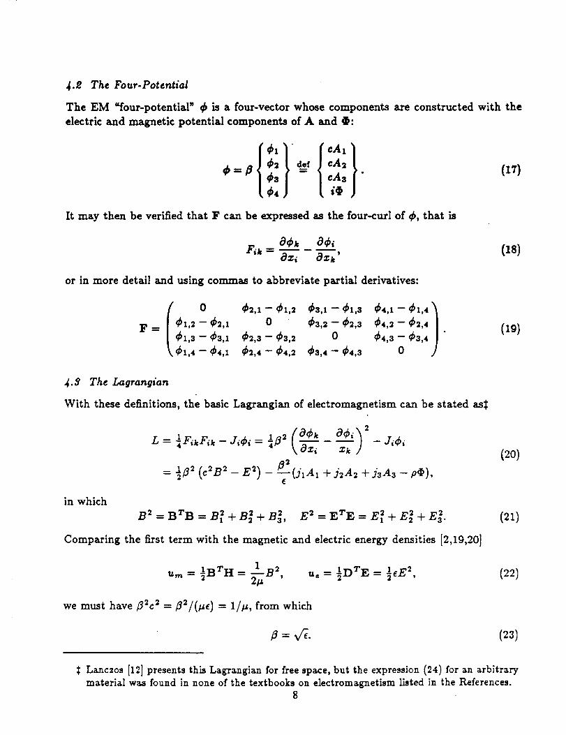
J.2 The Four-Potential

The EM _four-potential" _ is a four-vector whose components are constructed with the

electric and magnetic potential components of A and _:

{cA,}cAs "

iO

It may then be verified that F can be expressed as the four-curl of _, that is

(17)

ack (18)Fik = Ox_ axk'

or in more detail and using commas to abbreviate partial derivatives:

-- _1_2,1 0 ¢3,2 _2,3 _4,2 _2,4 •)F=

k._1,4 _4,1 ¢h,4 _4,= _s,4 ¢4,s o

(19)

_.3 The Laqranqian

With these definitions,the basic Lagrangian of electromagnetism can be stated as_

L 1 1210(_k O_)i_ 2= - = -- - J_i_F,_F_k J_ _ Oz_ zk /

_2= ½/32 (c2B 2 - E 2) - -_"(jlA1 + j2A= + jsAs - a¢),

in which

B 2=BTB=B_+B22+B_, E 2=ETE=E_+E22+E_.

Comparing the firstterm with the magnetic and electricenergy densities [2,19,20]

1 T 1 2u,_ = ½BTH = I---B2, u, ]D E == ]_E ,

2p

we must have/32c 2 = B'_/(.e) = 1//_, from which

(20)

(21)

(22)

= vq. (23)

t Lanczos [12]presents thisLagramgian for freespaxe, but the expression (24)for an arbitrary

material was found in none of the textbooks on electromagnetism listedin the References.

8

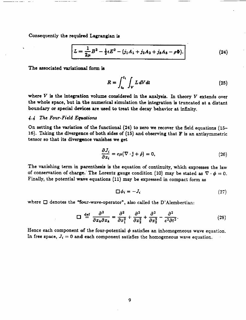
Consequently the required Lagrangian is

[ L -" _-_B2 - ½eE2 - (jIAI + j2A_ + jsAs - pO). ] (24)

The associated variational form is

R ffi f., dVdt (25)

where V is the integration volume considered in the analysis. In theory V extends over

the whole space, but in the numerical simulation the integration is truncated at a distant

boundary or special devices are used to treat the decay behavior at infinity.

4.4 The Four-Field Eqttations

On setting the variation of the functional (24) to zero we recover the field equations (15-

16). Taking the divergence of both sides of (15) and observing that F is an antisymmetric

tensor so that its divergence vanishes we get

o=-'-:.= _.(v. j + _) = 0, (2_)

The vanishing term in parenthesis is the equation of continuity, which expresses the law

of conservation of charge." The Lorentz gauge condition (10) may be stated as V • _b = 0.

Finally, the potential wave equations (11) may be expressed in compact form as

I-I_ = -Ji (27)

where [] denotes the "four-wave-operator', also called the D'Alembertian:

def 0 2 0 2 0 2 0 2 0 2

o = a=ka=k= _ +_ + a=_ _at=" (2s)

Hence each component of the four-potential _b satisfies an inhomogeneous wave equation.

In free space, Ji = 0 and each component satisfies the homogeneous wave equation.

9

5. THE AXISYMMETRIC TEST EXAMPLE

The simplest example for testing the finite element formulation based on the four-potentiaI

variational principle is provided by the axisymmetric magnetic field generated by a uniform,

steady current flowing through a straight, infinitely long conducting wire of circular cross

section. In the present Section we derive expressions for the magnetostatic fields outside

and within the conductor. These analytical solutions will be later compared with the finite

element numerical solutions.

5.1 The Free.Space Magnetic Field

To take advantage of the axisymmetric geometry we choose a cylindrical coordinate system

with the wire centerline as the longitudinal z-axis. The vector components in the cylindrical

coordinate directions r, 0 and z are denoted by

At, Bt, E1

A2, B2, E2

A3, B3, E3

in the r direction

in the 0 direction

in the z direction

The electromagnetic fields will then vary in the radial direction (r) but not in the angular

(0) and axial (z) directions. Similarly, the current density that flows in the wire has only

one nonzero component acting in the positive or negative z direction; conventionally we

select the positive direction.

In Cartesian coordinates the radial component of the electrostatic potential in free space

can be calculated from the expression (see, e.g.,[2,10,18,19,20])

fv jsA,- As----47r _ dV, (29)

where Irlisthe distance between the elemental charge J3 dV and the point in space at which

we wish to find the fieldpotential. The integralextends over the volume containing charges.

This expression serves equally well in cylindricalcoordinates. In fact, the transformation

of z components will be one to one ifthe center of the systems coincide.

As noted above the only non-vanishing component of the current vector isJ3 dS where dS

isthe elemental cross sectional area of the conductor and J3 isthe current density in the z

direction. If dL represents the differential length of the wire, then fs js dV = fs Js dS d_ =

I d£ = I dz and [r[ = v_r 2 + z 2. Substitution into Eq. (29) yields

uoI dz= .-oo + (30)

This integral diverges, but this difficultycan be overcome by taking the wire to have a

finitelength 2L symmetric with respect to the fieldpoint, that is large with respect to its

diameter. Integrating between -L and +L we get

A3(r)= _ t.v/ri+z: -'_ln z+v/r 2+z 2 .10

(31)

Expanding this equation in powers of r/L and retaining only fLrst-order terms gives

where C is an arbitrary constant. For subsequent developments it is convenient to select

C = (#oI/2_') inRT, where RT is the _truncation radius n of the finite element mesh in the

radial direction. Then

As = \_/in _ . (33)

With this normalizatima As = 0 at r = Rr. Taking the curl of A gives the B field in

cylindrical coordinates:

B=VxA= B2 = Bo = _r

O(,A_)Ia_A,A oB3 B. lr Or - r O0

It isseen that the only non-vanishing component of the magnetic flux density is

(34)

Bo - B2 = #o112 = ---OAz #oI

= -- (35)Or 2_rr"

This expression iscalled the law of Biot-Savart in the EM literature.

5.2 Magnetic Field Wi_'n the Conductor

Again restrictingour consideration to the staticcase, we have from Maxwell's equations

in their integral flux form

/c H" ds =/c#-IB" ds =/sj • dS, (36)

where C is a contour around the field point traversed counterclockwise with an oriented

differential arclength ds and dS is the oriented surface element inside the contour. The

term for the electric field disappears in this analysis because ]_ = 0. From before we know

that the right hand side of Eq. (35) is equal to the normal component of the current that

flows through the cross sectional area evaluated by the integral. In the free space case, this

is the total current that flows through the conductor. But in the conductor the amount

of current is a function of the distance r from the center. Again using I to represent the

total current carried by the conductor, and R the radius of the conductor, and assuming

an uniform current density 3"3 = I/(TrR2), the right hand side of (35) become_A

J_$ /S I /S rj. dS = JsdS = _-_ dS = I_-_.I1

(37)

Evaluating the left hand side of the integral and solving for B2 gives:

2¢•_-xB2 = I_-_, B2 = _I,- (38)2=R2"

Comparing with (34) we see that if # = _o then B2 is continuous at the wire surface 1, = R

and has the value _ol/(2_rR). But if _ _ _o there is a jump (_ - _o)I/(21rR) in B2.

The magnetic potential As within the conductor is easily computed by integrating -Bz

with respect to r:

#I• 2

A3 = 4re.R2 + C. (39)

The value of C is determined by matching (33) at • = R, since the potential must be

continuous. The result can be written

(40) ¸

The preceding expressions (33)-(40) for As could also be derived in a somewhat more direct

fashion by integrating the ordinary differential equation V2As = r-l(8(r0As/(gr)ar) =

#is to which the second of (11) reduces.

6. FINITE ELEMENT DISCRETIZATION

6.1 The Lagrangian in C_lindrical Coordinates

To construct finite element approximations we need to express the Lagrangia.n (24)

L = - - pc),

in terms of the potentials written in cylindrical coordinates.

expression of the curl (33)

B2 = (! °_4s- OA 2 )2(9z + _( _-A z(gz (ga s _ 2_r) + ( ! (9 (rA 2)or

For E 2 we need the cylindrical-coordinate gradient formulas

a+'A }i0@ , j

E= E2 = Ee =- F_'r"_2 ,

Ez E, 8@ + Jt-37 3

so that

E2 ET E (9(I) I (9(I) 2 O_(I) 3= = +-- + _+-- + +--

12

(4i)

For B 2 we can use the

21 aA1 (42)r (ge '

(43)

(44)

In the axisymmetric cue, Ax - A2 - 0; furthermore Az -- As is only a function of the

radial distance from the wire. Therefore aAa/aO = aAa/az = 0. From symmetry consid-

erations we also know that the electric field cannot vary in the 0 and z directions, which

gives a_/Sz = 8_/80 ---- 0. Finally, the only nonvmaishing current density component is

is. Consequently the I, agrangian (41) simplifies to

L = _ k O,./ - ½' _T + k-g/-/ - (y,a, - p_). (45)

6._ Conatructing EM Finite Elemer.t8

To deal with this particular axisymmetric problem a two-node "line * finite element ex-

tending in the radial r direction is sufficient. -In the following we deal with an individual

element identified by superscript e. The two element end nodes are denoted by i and j.

The electric potential • and the magnetic potential As - Az are interpolated over each

element as

0" -- N00", i_ -- N_A._, (46)

Here row vectors N 0 and N_t contain the finite element shape functions for _e and A_,

respectively, which are only functions of the radial coordinate r:

N0 = (N&(0 N&(0), N_ = <N_(,) N_,;(,)), (47)

and column vectors 0 e and A_ contain the nodal values of @ and As, respectively, which

axe only functions of time t:

Oe = {@i(t) } {Azi(t)} (48)_,;(t) ' A_= a_;(t) "

Substitution of these finite element assumptions into the Lagrangian (45) and then into

Eq. (25) yields the variational integral as sum of element contributions R - _"_e Re, where

R e ---

(49)

where V e denotes the volume of the element. Taking the variation with respect to the

element node values gives

. \ Or Or A'_+e(NeA)TN'A_L;--J3(NeA)T

i,;'S.[+ . (_,)r -'k a, / a,

(so)

13

On applying fixed-end initial conditions at t = to and t = tl and the lemma of the calculus

of variations, we proceed to equate each of the expressions in brackets to zero. From the

first bracket we obtain for each element the following second-order dynamic equations for

the magnetic potential at the nodes, which are purposedly written in a notation resembling

the mass-stiffness-force equations of mechanics:.

M_ + K_A_ = f_, (51}

where

MeA = Iv, ((N_) T N_ dV', /v 1 ((gN_t_ T ON_K_= ._ \ ar / _ dV', (52)

y_(N_)T_v'. (53)

From the second bracket we obtain for the electric potential a simpler relation which does

not involve time derivatives, i.e, is static in nature:

K;®" = f_, (54)

where

K_= ._\ a, / _ av', f_= . o(N_) r av'. (ss)

Assembling these equations in the usual way we obtain the semidiscrete master finite

element equations:

MAA3 + KAA3 = fA, (56)

K®_ = f_.

6.8 The Static Case

In time-independent problems, the term _1.3 disappears from (56) and the master finite

element equations of electromagnetostatics become

KaA3 =fa, K®@ = fv. (57)

If the current density and charge distributions are known a priori then these two equations

may be solved separately. If only the charge distribution p is known then the second

equation should be solved first to obtain the electric field E as gradient of the computed

electric potential @; then the current density j can be obtained from Ohm's law (6) and

used to computed the force vector fa of the first equation, which is then solved for the

magnetic potential. Conversely, if only the current density distribution is known a priori

the preceding steps are reversed.

For the present test problem the current distribution is assumed to be known, and we shall

be content with solving the first equation for the magnetic flux.

14

6.._ An Altcrnatine Scmidiacretizalion

If upon setting the brackets of the variation (50) to zero we multiply them through by

and 1/_, respectively, the expressions for the mass, stiffness and force matrices become

M_- • _-_ (N_)T-N_ dV', K_- o \ ar ) "_e dV ' f_ - . PjsN_T dg*'

fv ( T f; = fv ";z•k a, / .. dV.

(ss)The matrices M and K above are quite similar to the capacitance and reactance matrices,

respectively, obtained in the potential analysis of acoustic fluids [7,8]. Another attractive

feature of (58) is that Kx "- Ke if the shape functions of both potentials coalesce, as is

natural to assume. These advantages are, however, more than counterbalanced by the fact

that _jump forces n contributions to fA and f@ arise on material interfaces where _ and

E change abruptly, and the proper handling of such forces substantially complicates the

programming logic. Note that this issue does not m'ise in the treatment of homogeneous

acoustic fluids.

6.5 Applying Boundary Condition8

The finite element mesh is necessarily terminated at a finite size, which for the test prob-

lem is defined as the truncation radius R_ alluded to in Section 5.1. In static calculations

the material outside the FE mesh may be viewed as having zero permeability/_, or, equiv-

alently, infinite stiffness or zero potential. It follows that the potential value at the node

located on the truncation radius may be prescribed to be zero. This is the only essential

boundary condition necessary for this particular problem.

7. NUMERICAL VALIDATION

7.1 Finite Element Model

The test problem consists of a wire conductor of radius R transporting a unit current

density. For this problem the finite element mesh is completely defined if we specify the

radial node coordinates r_ = r_ and r_ = rn+ze for each element e. If the mesh contains Nec

elements inside the conductor, those elements are numbered e = 1, 2,... Nec and nodes

n -- 1, 2, ... !V_c + 1 starting from the conductor center outwards. The first node (n = 1)

is at the conductor center r = 0 and node n = -N'ec + 1 is placed at the conductor boundary

r ---- R. The mesh is then continued with Ne/ elements into free space, with a double

node at the counductor boundary. The last node is placed at r = RT at which point the

free space mesh is truncated; usually RT = 4R to 5R. Although the mesh appears to be

one-dimensional, a typical element actually forms a _tube n of longitudinal axis z, internal

radius r_ and external radius r_, extending a unit distance along z.15

1. loe

e. 888

e.m

0.2Re

e.eee

e. eee

w

_'%\k

\\\

\\

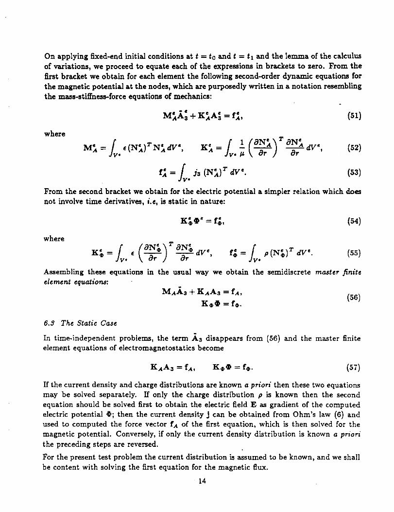
Figure 1.

1.eee _.eee r 3.8ee 4.eee 5.e88

Magnetic potential As vs. distance from center r,/_,_,, = 10.0: finite

element values (triangles) and analytical values (squares).

e. _eo

0.3_0

0.:_0

A3

O. 160

O. 080

\

",\

\-,=

a.

"a_.m.

0.000 1 I ! ' t I

C.OOO 1.000 :._eO r 3.oee 4.eoe s.ooe

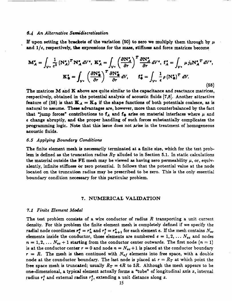
Figure 2. Magnetic potential As vs. distance from center r, /_,e = 1.0: finite

element values (triangles) and analytical values (squares).

16

1 • ?@0

1.380

1.e_e

B2

e. 680

@o340

0._

//

II

I

//

/I

/11

.t

', ,-"-'_,_-_'--'T_-_ ,-_---r--,_-.-_

0.000 1.000 2.000 r 3.000 4.000 5.000

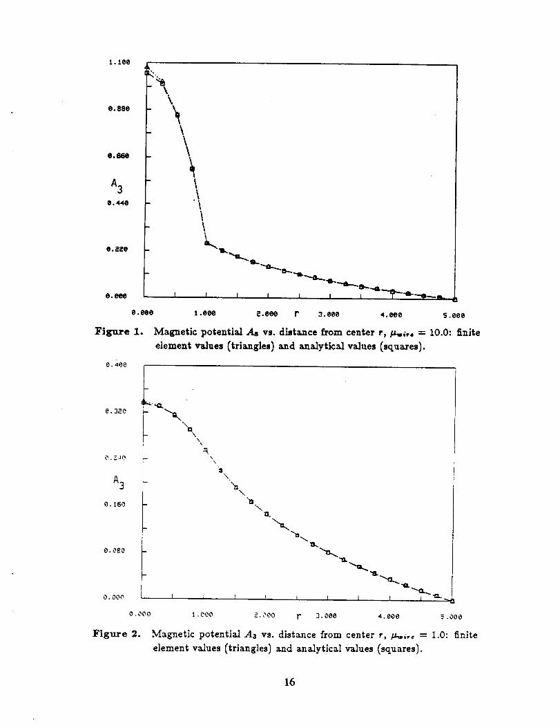
Figure 3.

0.170

Mai_etk _11x density B= vs. distance from center r, /_,_,, = I0.0:finite element value. (triangles) and analytical values (squares). Valuesshown on the interface r = 1 with dark symbols have been extrapolated

from ekment center values to display the jump more accurately; thisextrapo|Mion scheme has not been used elsewhere.

0.136

0. 102

B2

0. 068

0.034

0.000

/ \I

/

J/

//

_ /:7

//

\.

\

m.

I I I I I 1 I I

0. 000 1.000 2.000 r 3.000 4.000 5.000

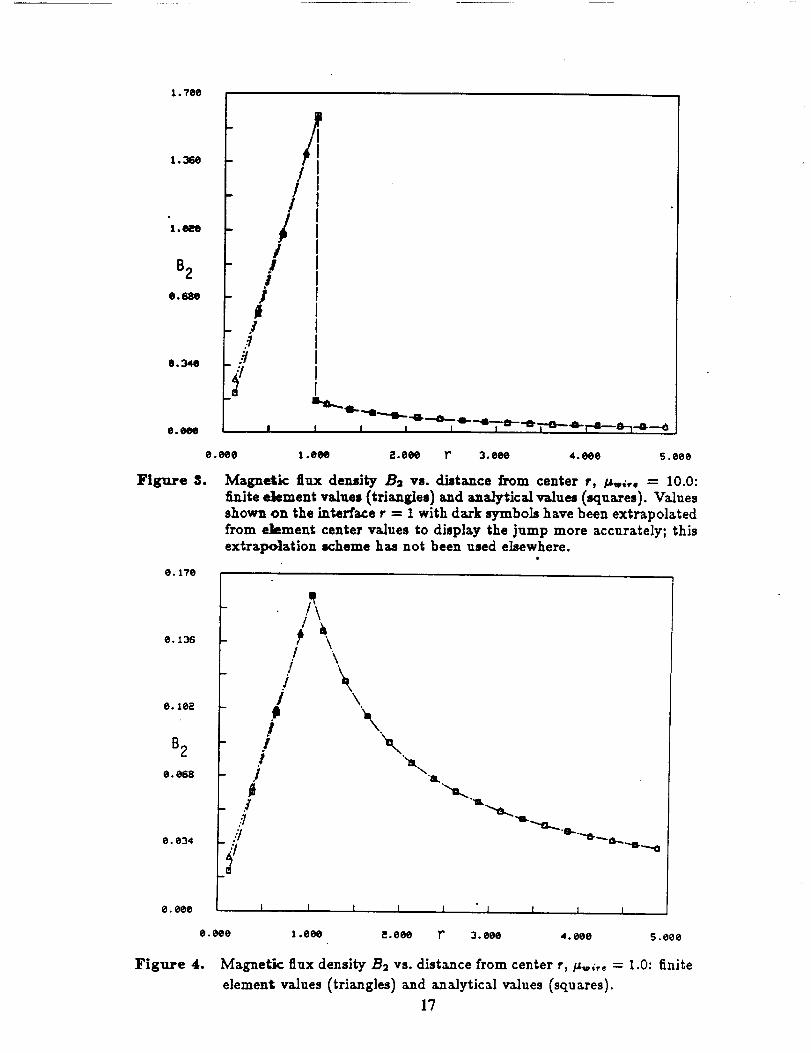
Figure 4. Magnetk flux density B2 vs. distance from center r, _;. = 1.0: finite

element vaJues (triangles) and analytical v_lues (squares).

17

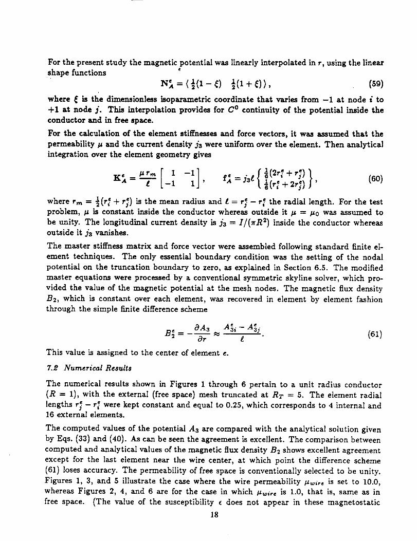
For the present study the magnetic potential was linearlyinterpolated in r, using the linear

shape functions

1N_=(½(1-_) ½(1+_)), (59)

where _ is the dimensionless isoparametric coordinate that varies from -I at node i to

+1 at node j. This interpolation provides for C o continuity of the potential inside the

conductor and in free space.

For the calculation of the element stiffnessesand force vectors, it was assumed that the

permeability # and the current density J3 were uniform over the element. Then analytical

integration over the element geometry gives

= --T- =/31 + ,;) (6O)__ , 1 e 2r_) '+

where rm -- ½ (r_ + r_) isthe mean radius and l = r_ - r_ the radial length. For the test

problem, # is constant inside the conductor whereas outside it # - #o was assumed to

be unity. The longitudinal current density isd3 = I/(7rR2) inside the conductor whereas

outside itjs vanishes.

The master stiffnessmatrix and force vector were assembled following standard finiteel-

ement techniques. The only essential boundary condition was the setting of the nodal

potential on the truncation boundary to zero, as explained in Section 6.5. The modified

master equations were processed by a conventional symmetric skyline solver, which pro-

vided the value of the magnetic potential at the mesh nodes. The magnetic flux density

62, which is constant over each element, was recovered in element by element fashion

through the simple finitedifferencescheme

OA3 (61)a--;-- l

This value is assigned to the center of element e.

7.2 Numerical Results

The numerical results shown in Figures 1 through 6 pertain to a unit radius conductor

(R = 1), with the external (free space) mesh truncated at Rr = 5. The element radial

lengths r_ - r_ were kept constant and equal to 0.25, which corresponds to 4 internal and16 external elements.

The computed values of the potential As are compared with the analytical solution given

by Eqs. (33) and (40). As can be seen the agreement is excellent. The comparison between

computed and analytical values of the magnetic flux density B2 shows excellent agreement

except for the last element near the wire center, at which point the difference scheme

(61) loses accuracy. The permeability of free space is conventionally selected to be unity.

Figures 1, 3, and 5 illustrate the case where the wire permeability #_i,_ is set to 10.0,

whereas Figures 2, 4, and 6 are for the case in which #to,re is 1.0, that is, same as in

free space. (The value of the susceptibility ( does not appear in these magnetostatic

18

e. 170

e.136

e. le2

8 2

e. 068

e. e34

6.eee

e.se6

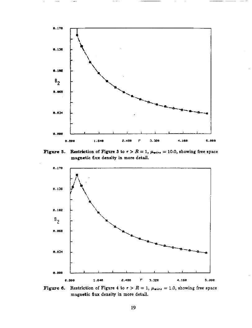
Figure 5.

e. 176

\\

\

\\

'lt'_3a,_ "

| I l I I I I I 1

1.646 2.48e r" 3.3_6 4.166 S .666

Restr_tion of Figure 3 to r > R = 1,/_;,, = 1O.0, showing free 6pace

magnetic flux density ]n more detail.

6. 136

0. 102

B2

e. 668

6. 634

e. 6e6

F]gure 6.

q

/\\

\

\

\\

"tt"" -11..... a,.. -

I I I I I I I I I

6.8ee 1.64e 2.486 r 3.3_6 4. 166 5.666

Restriction of Figure 4 to • > R = 1, _,;,o = 1.0, showing free space

magnetic flux density in more detail.

19

computations.) Figures 1 and 2 show computed and analytical magnetic potentials. The

slope discontinuity at r - 1 in Figure 1 is a consequence of the change in permeability

from the wire material to free space. Figures 3 and 4 show the computed and analytical

magnetic flux densities. As discussed in Section 5.2,the jump at r - 1 in Figure 3 is due

to the change in permeability _ from the material to free space. Figures 5 and 6 show the

computed and analytical magnetic flux densities in free space with more detail. Note that

Figures $ and 6 for r > 1 are identical; this is the expected result because, as shown in

Section 5.1, the free-space magnetic flux field depends only upon the current enclosed by

a surface integral around the wire and not on the details of the interior field distribution.

In summary, the finite element model performed very accurately in the test problem and

converged, as expected, to the analytical solution as the size of the elements decreased.

8. CONCLUSIONS

The resultsobtained in the one-dimensional steady-state case are encouraging, and appear

to be extensible to two- and three-dimensional problems without major difficulties.The

electricfieldremains effectivelydecoupled from the magnetic fieldexcept through Ohm's

law. Care must be taken, however, in modeling the forcing function terms so as to avoid

the appearance of discontinuity-induced forces at physical interfaces.

The next step in achieving the goal of a finiteelement model for a superconductor fieldisto

study the time-dependent case, starting with harmonic currents and proceeding eventually

to general transients. The code for this is currently written, but a suitable analytical

solution for comparison with computed responses is stillbeing developed.

If encouraging results are obtained in the dynamic case, thermocoupling effectswill be

added to the code. References [3,17,22]discuss several differentapproaches applicable to

various contexts (e.g. eddy currents) and these will have to be investigated for suitability

for capturing the couplings effectsthat are relevant to the superconducting problem.

After modeling the coupling effects,the next step will be to model the superconducting

fields.The feasibilityof using the current model for superconductor applications ksgreat,

as the current density of a superconductor can be approximated by the standard current

density multiplied by a constant squared. This constant is called the London penetration

depth. Other analytical models that possess similar characteristics have been developed

and are presented in Ref. [11].

2O

Acknowledsements

Thk work wM supported by NASA Lewis Research Center under Grant NAG 3-984, monitoredbyDr. C. C. ChaJnis.

Io

*

3.

.

.

.

.

.

10.

11.

12.

13.

14.

REFERENCES

Davies, J. B., The F'mite Element Method, Chapter 3 in Numerical Techn/ques/or Microwave

and Millimeter. Waee Passive Structures, T. Itoh (ed.), Wiley, New York, 1989

Eyges, L. The Claaffcal Eleefromafnetic Field, Dover, New York, 1980

Fano, R.M., Chu, L.J., and Adler, R.B., Electromagnetic Fiel&, Enerfv, and Forces, JohnWiley and Sons, Inc., New York, 1960

Felippa, C. A. and Geers, T. L., Partitioned Analysis of Coupled Mechanical Systems, Engi-

neering Computations, 5, 1988, pp. 123-133

Felippa, C. A., The Extended Free Formulation of Finite Elements in Linear Elasticity,

Journal o.f Applied Mechanicj, 86, 3, 1989, pp. 609-616

Felippa, C. A. and _d_Utel]o, C., The Variational Formulation of High-Performance Finite

Elements: Parametrized Variational Principles, (with C. ]vfilitel]o), submitted to Computers

Structurea, 1989

Felippa, C. A. and MiBtello, C., Developments in Variational Methods for High-Performance

Plate and She]] Elements, to be presented at the ASME Winter Annual Meeting, San Fran-

cisco, December 1989"

Felippa, C. A. and Ohayon, I%. Treatment of Coupled Fluid-Structure Interaction Problems

by a ]vfixed Variational Principle, Proceedinga 7th International Con/erence on Finite Ele-

ment Method8 in Fluids, ed. by T.J. Chung et._/., Univer-qity of Alabama Press, Huntsville,

AJabama, April 1989, pp. 555-563

FelJppa, C. A. and Ohayon, R. l_fixed Variational Formulation of Finite Element Analysis

of Acousto-elastic Fluid-Structure Interaction, submitted to Journ_ o/Fluids e/Structures,1989

Grant, I.S., and Phillips, W.R., Electromagnetism_ John WHey and Sons, Inc., New York,1975

Kittel, C., Introduction to Solid State Philsica, 6th. ed, John Wiley and Sons, Inc., New York,1986

Lanczos, C. The Variational Principles o/MecAanics, Univ. of Toronto Press, Toronto, 1949

Lorentz, H. A., TheorF o/Electron_, 2nd. ed, Dover, New York, 1952

MJliteilo, C. and Felippa, C. A., A Variational Justification of the Assumed Natural Strain

Formulation of Finite Elements: I. Variational Principles, (with C. ]Vfilite]]o), submitted to

Computer_ _YStructure_, 198821

15.

18.

17.

18.

19.

20.

21.

22.

l_E_tl/tello, C. and Felippa, C. A., A Variational Justification of the Assumed Natural Strain

Formulation of Finite Elements: ]I. The C"° 4-Node Plate Element, submitted to Computer_Structurea, 1988

Park, K. C. and Felippa, C. A., Partlt]oned Analysis of Coupled Systems, Chapter 3 in

Computah'onal _fothods/or _aruient Anaivaia , T. Be]ytschko and T. J. R. Hughes, eds.,North-Holland, Amsterdam-New York, 1983

Parkus, H., ed., Electromagnetic lrderacfiona in Elaatic Soil&, Springer-Verlag, Berlin, 1979

Purcell, E-M., ElectricitV and Magneti:m, Vol. 2, McGraw-Hill, New York, 1985

Rojanski, V., The Electromagnetic Field, Dover, New York, 1979

Shadowitz, A. The Electromagnetic Field, Dover, New York, 1975

Trowbridge, C. W., Numerical Solution of Electromagnetic Field Problems in Two and Three

Dimensions, Chapter 18 in Numerical Methods in Coupled Problem_, ed. by R. Lewis eLaL,Wiley, London, 1984

Yuan, K.-Y., Moon, F. C. and Abel, J. F., Elan, tic Conducting Structures in Puked Magnetic

Fields, Chapter 19 in Numerical Methods in Coupled Problenu, ed. by R. Lewis et.ai., Wiley,London, 1984

22

APPENDIX: COMPUTER PROGRAM

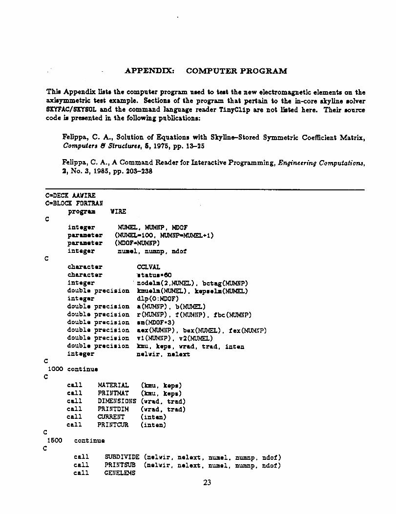
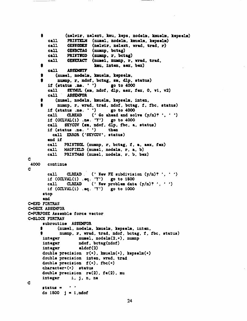
Thk Appendix lists the computerprogram usedto test the new electromagneticelementson the

aockymmetric test example. Sections of the program that pertain to the In-core skyline solver

SKYFAC/Sq_YSOL and the command language reader TlnyClip are not lkted here. Their source

code k presented in the following publications:

Fel]ppa, C. A., Solution of Equations with Skyline-Stored Symmetric Coe_cient Matrix,

Computera _ Strudurea, 5, 1975, pp. 13-25

FelJppa, C. A., A Command Reader for Interactive Programming, En_neeri.y CompufaHon_,

2, No. 3, 1985, pp. 203-238

C=DECK AAWIREC=BLOCE FORTRAN

programC

integerparameter

parameter

integerC

C1000

C

C

1500C

¥II_E

MUMEL. MUMI_, MDOF

(_OF=_)

mmel. nu_up, ndof

character

character

integer

double precision

integer

double precision

double precision

double precisiondouble precision

double precision

double precision

integer

CCLVAL

status*60

nodela(R.MUMEL), bc_ag (MUMNP)kzmela(MUMEL), kepselm(MUMEL)dlp(O :MDOF)a(_fl_4NP).b(_FO}4EL)

r(_UM_P), f(_), fbc(_P)amCMDOF*3)aex(MUMNP), bex(MUMEL), fex(MUMNP)

kmu, keps, wrad. trad. intennelwir, nelext

continue

call MATERIAL (]mu. keps)

call PRINTMAT (kmu, keps)call DIMENSIONS (wrad. trad)

call PRINTDIM (wrad. trad)call CURRENT (intan)call PRINTCUR (inten)

continue

call

call

call

SUBDIVIDE (nelwir, nelext, numel,

PRINTSUB (nelwir. nelex_, numel.GENFIENS

23

numnp, ndof)numnp, ndof)

$

$

$$

$$

(nelwir. nell. htuo kepe0 models. _nuelu. kepseln)call PRIFFELMcall GEHODEScall G_AGcall PRIIFri_D

call GEgEXACT

call ASSEMSTF

(nunel0 models0 Enuolm. kopselm)(nelwir. nelex_.._-td, trad. r)

(numnp, bctq)

(nunmp. r. bctq)(m-el. nuunp, r. wrad. trad._u, inten° aaXo bex)

call

end if

call

callcall

C

(nuael, n_lela, _uels, kepselm,

=p, r, Idol, bctq, 8a, dip, sat.tun),tf (s.Ca.Cu8 .no. ' ') go 'to 4000call KYMUL (an. ndof, dlp. sex, rex. O, vl, v2)call ASSEMFOK

(nunel. models, 1,:nuelm. kepseln. In.con.

nuunp, r. vrad. fred, ndof. bctq0 f. fbc. ate.cue)

if (s.catu8 .no. ' ") go to 4000

call CLREAD (" Go ahead and solve (y/n)? ', " ")if (CCLVAL(1) .me. "Y') go to 4000

call SKYCOV (an, ndof, cLIp, fbc, a, s.catus)if (status .me. ° ") .chert

ERR_K ('SKYCOV', Status)

PRINTSOL (numnp, r, bctq0 f0 t, aex, fmc)NAGFIELD (nuael, models, r. a, b)PRINTMAG (nuael, nodelm, r. b. bex)

4000 continue

C

call CLREAD (' hv FE subdivision (y/n)? ', ' ')if (CCLVAL(1) .ca. 'Y') go to leO0

call CLREAD (' Rev problem data (y/n)? ', ' ')if (CCLVALC1) .oq. 'Y') go to 1000

atopend

C-END FORTRAN

C=DECK ASSEMFOR

C:PURPOSE Assemble force vectorC=BLOCK FORTRAN

subroutine ASS_D4FOR

@ (numel, nodal=, kmuelm, kepselm, intau.

$ numnp, r, wrad, trad, ndof, bctag, f, fbc, status)integer nunel, models(2,*), numnpinteger rider, bctag(ndof)integer elder (2)

double precision r(*), kmuelm(*), kepselm(*)double precision inten, wrad, traddouble precision f(*), fbc(*)character* (*) st atuJ

double precision re(2), re(2), mu

integer i, j o n, ne'C

sJ;a_us - ' '

do 1500 j - 1,ndof

24

1500C

22O0

C

25OOC

3000

:_(j). o.ocont inue

do 8000 ne - 1,n_seldo 2200 i - 1,2

n - nodelaC:L ,_e):e(i) - r(n)eldofCi) - ncontinue

nu - _uela(ne)call FORCE (he, re, tnten, wrad, re, stature)

if (status .he. ' ') thencall _q,.ROR ('ASSDOFOR', status)

end if

do 2500 £ - 1,2

J - eldof (i):(J) - :CJ) *:e(_)cent inue

cent inue

do 4000 j = 1,rider

fbcCJ) - :(J)if (bctag(j) .he. o) _bc(_) -o.o

4000 cent inuereturn

endC:END FORTRAN

C--DECK ASSEMSTF

C:PURP0SE Assemble master stiffness matrix

C=BLOCK FORTRANsubroutine ASSEMSTY

$ (numel. nodelm, kzuel_, kepselm.

$ numnp, r. rider, bctag, sin. cLIp. status)character* (*) status

integer numel, nodelm(2,numel), num_p

integer ndof. bctag(ndof), dlpC0:ndof)double precision kmuelm(numel), kopselm(numel)

double precision r(ndof), sm(*)double precision re(2), sme(2,2)integer elder C2)

integer i, _, k, li, _J. n. me

C

¢

Status = ' '

2500

C

call PORMDLP (numel. nodelm, ndof, bctag, dlp)

do 2500 i - 1,abs(dlp(ndof))

smCi) = 0.0

cont inue

do 4000 ne : 1,numel

do 2200 i : L,2n = nodelm(i ,ne)

25

2200" C

C

350036OO

C4000 continue

Creturn

endC=END FORTRAN

C=DECK CURRENT

re(1)- rCn)elder(1) - ncontinue

c8_1 STIFF Cue, re, ]muelnCne). one, status):Lf (stal;us .so. " ') then

call ERa01 ('AS_'. status)end if

do 3600 i - 1,2_i - elder(1)

do 36_ J " t.2jj - e].a._(j)i_ (JJ .Is. ll) than

k- _.BCdlpCii)) - ii + JJsuck) - suck) + sueCi,J)

_d if

continue

continue

C-PURPOSE Read current intenslt 7C-BLOCK FORTRAN

subroutine CURREST (intan)

double precision DCLVAL

double precision lntencall CLREAD (' Enter current inten_itT: '. ' ')

intan - DCLVAL(I)return

end

C=END FORTRAN

C=DECK DIMENSIONS

C=PURPOSE Read problma dimensions (wire and truncation radius)C=BLOCK FORTRAN

subroutine DIMEmSIONS (wrad, trad)

double precision DCLVALdouble precision wrad. tradcallwrad mtrad -return

endC=END FORTRANC=DECK ERRORC=PURPOSE Fatal error termination subroutineC=BLOCK FORTRAN

subroutine ER3.0R (name, me|aS_e)

character*(*) name, message

CLREAD (" Enter vire radius, trunc radius: ', ' ')

DCLV*L(1)DCLVAL(2)

26

Cinteger i, I

I = len(aemsage)

do 1200 i = lea(message).1,-1

if (aemmage(i:i) .he. ' ') go to 1300

i- i

1200 coat Anus

1300 continue

print *, ' '

print *, '*** Fatal error condition detected ***'

print *, aeesage(l:l)

print *, 'Error detected by ', name

stop '*** Error stop ***'end

C=EI_D FORTI_N

C:.DECX FORCE

C=PURPOSE Compute node forces for axisTmm EM element due to jC=BLOCK FORTRAN

subroutine FORCE

$ (he, re, inten0 wTad, re, status)

int seer no

double precision re(2), inten, wrad, re(2)character* (*) status

double precision ri, rj, re, fnC

status m . .

ri - re(l)

rJ " re(2)

if (rJ .le. ri) thenwrite (status, "(A,I5) ')

$ 'FORCE: Negative or zero length, element' .noreturn

end if

rm " O. 5" (ri+rj)if (r_ .It. wrad) then

fn - (int en/(3.14159*wrad** 2) ) * (rj -ri )

re(l) = fn* (ri+ri+rj)/6.

fe(2) - fn* (ri+rJ +rj)/6.else

re(l) = 0.0

re(2) = o.oend if

return

end

C=END FORTRAN

C=DECK FORMDL o

C=PURPOSE Form diagonal location pointer (DIP) arrayC=BLOCK FORTRAN

subroutine

8integer

integer

integer

FOPJ_DLP

(numel, nodelm, ndof. bctag, dlp)numel, nodelm(2,numel), ndof

bctag(ndof), dlp(0:*)

i. j, k, n, no, eldof(2), nsk"y

27

C

1200

1600

1800

2OOO

22OO

C

C

do 1200 £ - O.-,Ao_

dlp(i)- 0continue

do 2000 no - 1 .nuneldo 1600 £ ,, 1.2

n - no4e_,,(l .no)

eldo:t(t) - ncent inuo

do 1800 t . 1.2k " elder (i)

do 1800 ] - 1,2if (eZdo_(J) .I.e. k) "r,hendip(k)- na.x(dlp(k).k-eldof(J)+1)end i_cont_ue

cent inue

do 2200 i - 1,riderdlp(1) = _p(£-I) + _p(_)cant inue

risky = ab8 (ekZp(ndo_))

print ' (/' ' No ef equations : ' "o II0)' ,riderprint '('' Avtrqe bandwidth: ",F12.1)'.floatCnsky)/ndofprint '(" Entries to store skyline:",IlO)',nsk Tprint ' ( .... )'

do 3000 i - 1.ndqfi_ (bctagCi) .he. O)

3000 cont inueret_

endC=END FOI_TRANC-DECK GF/BCTAG

dlp(i) = -absCdlp(i))

C:PURPOSE Generate pot_tial BC data by fixing e_'tez-_oit nodeC:BLOCK FOB.TI_t_

subroutine GEMBCTAG (nunmp, bctag)integer numnp, bctag(*)

integer n

do 2000 n- 1,nnxnpbctag(n) - 0

2000 c on_ inue

bctag(nu=np) = 1rmt_end

C-END FORTRANC=DECK GE_ELD4S

C_URPOSE Generate element dataC=BLOCK FORTRAN

subroutine GF_ELD4S

$ (nelwir, nelex_, kau, kep8, nodela, k:uels, kepselm)

integer nelwir, nelex_

integer nx, n, ne, node_(2,*)

28

double precision kmu. kepe. kmuelm(*), kopselm(*)nm 0

no - 0

do 2000 nx- l.nelwirn- n+l

nodelm(1.ne) - n

nodela(2.no) - n+l

l_uela(ne) = l_ukepsela(ne) = keps

2000 continue

do 3000 nx - 1.nelaxt

1,,== n+ 1

no m no ÷ 1

nodelmCl.ne) = n

nodelm(2.ne) - n÷l

li_uela(ne) - 1.0

kepse:l_(ne) - 1.03000 cent lnue

return

end

C=END FORTRAN

C=DECK GEFEXACT

C=PURP0SE Generate exact magnetic potentlal/fleld solutionsC=BLOCK FORTRAN

subroutine GF/EXACT (numel, numnp, r, wrad, trad.

$ kmu, inten, aex. bex)

integer numel _ numnpdouble precision r(*). wrad. trad. kmu. lnten

double precision aex(numnp), bex(numel)

integer n. ni

double precision c, rmC

c = - (intan/(2*3. 1415g) )*logCwrad/trad)

do 2000 n = 1.nunmpif (r(n) .It. wrad) then

aex(n) : (kmu*inten/(4*3.1415g_)) *(I. - (r (n) /wrad) **2) + c

else

aex(n) = -(inten/(2*3. 1415g)),log(r(n)/trad )end if

2000 cont inui

do 3000 ne = l,numel

rm = 0.5" (rCne) +rCne÷l))

if (rm .le. wrad) than

bex(ne) = (kmu*int en/(2,3.1415g) )* (rm/wrad** 2)else

bex(ne) = (inten/(2*3 14159))/rmend i_

3000 cont inue

ret_

end

C=END FORTRAN

C=DECK GF_ NODES

29

C-PUR_0SE Generate node date

C:BLOCX FORTRAN

subroutine GENIODES (nelvir, nelext, wrad, trad, r)

integer nel_r, nelex_

integer n, am

double precision wrad. t_rad, r(*)C

n- O

do 2000 ne - 1.nelvtr

n- n÷l

r(n) " (he-l) twrad/nelwlr

2000 continue

r(n+1) - _mddo 3000 ne - 1.aalext

n m n÷ 1

r(n) - vTad ÷ (ne-1)*(trad-_rad)/nelext

3000 cent inue

r (n+l) - trad

return

end

C=E_D FORTRAN

C:DECK MAGFIELD

C=PURPOSE Compute_l _etlc field (B) at element center

C=BLOCK FORTRAN

subroutine MAGFXELD (nuael. nodal:, r. a. b)

integer nuael, nodela(2.mmel)

double precision r(*). a(*). bCnuael)

integer ne. hA. njC

do 2000 ne - loauael

ni - nodes:(1 .he)

nj = nodel:(2.ne)

bCne) = -(a(nJ)-aCni)) ICrCnj)-r (ni))

2000 cont inue

retu_---n

end

C=END FORTRAN

C=DECK MATERIAL

C:PURPOSE Read material propertiesC'_BLOCK FORTRAN

subroutine MATERIAL (kmu, kep8)

double precision kmu. keps

double precision DCLVALcall

kzu-

kep8 =return

end

C=END FORTRAN

C=DECK PRINTCUR

C=PURPOSE Print current intensity

C=RLOCK FORTRAN

subroutine PRIFTCUR (inten)

CLREAD (" Enter kmu, keps for wire: ', " ")DCLVALCDDCX.VAL(2)

3O

double precision lnten

print ' (' " Current intensity: " ",FIe.3) ",intenreturn

end

C-END FORTRA_

C,,DECK PRIFI'DIH

CnPURPOSE Print problem diuenmions (wire and truncation radius)C_BLOCX FORTRAN

subroutine PP_FrDIN (wrad, trad)

double precision wrad, trad

print ' (" ' Wire radius : ' ' ,F10.3) ' ,wrad

print ' ("" Truncation radius : ' ' ,FlO.3)" ,tradreturn

end

C-END FORTRAN

C=DECK PRI NTELM

C-PURP0SE Print element dataC=-BLOCK FORTRA_

subroutine PI_FTEI_ (numel, nodelm, kmuelm, kepeelm)

integer i, n, numel, nodolm(2,*)

double precision kmuelm(*), kepselu(*)print *. '

print *. ' E 1 • m • n t D a t a °

print *, '

print *0

$ ' Elau I J ]mu keps'do 2000 n ,, 1.numel

print '(3I 5.21:'9.3) '. n. Cnodelm Ci. n). i-l. 2). _unuelm(n) .keps elm(n)2000 cont inue

return

and

C=END FORTRAN

C=DECK PRI NTMAG

C=PURP0SE Print computed and exact maEnetic field (B)C=BLOCK FORTRAN

subroutine PRINTMAG (numel. nodelm, r. b. bex)

integer hUmS1, nodelm(2 .numel)

double precision r(*) ,b(numel).bex(numel)

integer no. ni. njC

print *, °

print *. ' N a g n • t i c F i • 1 d'

print *. "

print *.

$ ' Elms r-center Comp-B2 Exact-B2 '

do 2000 ne = l.numel

ni = nodelm(l ,ne)

nj = nodelm(2 .ne)

print "(IS,FlO.3.2Fll.4)',ne,O.5,(r(ni)÷r(nj)).

$ b(ne) .bex (ne)

2000 cont inue

return

end

31

C-END FORTRANC-DECE PKI FFMATC=P_POSE Pr£nt natezl_ properties used in problem(>,BLOCK FORTRA_

subroutine PRIITMAT (kay. keps)

double precision ]mu, kepe

print "(" ' Rel. permeability of wire (vacuul-S) : ' ' .FIO.$) ' .kluprint ' (' ' Rel. poz_Ltttvtty of wire (vacuum=l) : "' ,F10.3) ' .kepsreturn

end

C=E_D F01tTItAN

(>,DECK PRIFrIOD

C-PURPOSE Print element dataC=BLOCK FORTRAN

subroutine PRIFTWOD (numnp, r, bctag)

integer n. nnmnp, bctag(*)double precision r(*)print *. 'print *, ' W o d • D a t a'print *. 'print *. ' Node r-coord bctag"do 2000 n = 1,_p

print "(I6.F10.3.16)'. n,r(n) .bctag(n)2000 continue

rmtu_

end

C=EI_D FOKTRAI_C,,DECK PKI NTSOL

C_POSE Print computed, and exact solutionC-BLOCK FORTRAN

subroutine PRIFTSOL (hump, r, bctag, f. a, sex, rex)

integer n. hump. bctag(numnp)double precision r(numnp) 0 f(numnp)

double precision a(numnp) o aex(numnp), fex(numnp)J

print *, 'print *. ' C o m p u t • d S o 1 u t i o n'

print *. 'print *.

$ ' Mode r bet ag Comp-f or',

$ ' Comp-A3 Exact-A3 Exact-for'do 2000 n = 1.nulnp

print '(I6.FlO.3.I6.4Fll.4) ' .n. r(n) .bctag(n).$ f (n).a(n) jsex (n),fex (n)

2000 continue

retul'nend

C-END FORTRAN

C=DECK PRINTSUB

C=PURPOSE Print subdivision data

C=BLDCK FORTRANsubroutine PRINTSUB (nelwir. nelex_, numel, numnp, ndof)

integer nelwir° nelex_c, numel, numnp, ndof

prin_ '(' ' Subdivisions in wire :'',I6) ", nelwir

32

print ' (' ' Subdivisions in free space: ' 'print ' (" Number of elements : '' .I6)'

print ' ('' Number of node points : "' .I6)"print '(" Number of dofs :",I6)'rettur_end

C-DECX SK'YCOV

C-FL_POSE Cover routine for stiffness solver

C-AUTHOR C. A. Yelippa, March 1972C-VERSION November 1982 (Fortran 77)

C-TIIISVERSION Condenmed on November 86 for ME593

C-E_JIP94ENT Machine independentC=KE_0RDS solve okyline stiffness equationC=BLOCK ABSTRACTC

C

C

C

C

C

C

C

C=END ABSTRACT

C=BLOCK USAGE

CC

CCCCC

.I6)', nelext

• numel

. n-w.p• ndof

C

C

C N

C P

C DLP

C

C

C

C U

C STATUSC

C

C

C=E_D USAGE

C=BLOCK FORTRAN

SKYCOV is a cover routine that solves the master

stiffness equation_K u " f

SEYCOV calls SKYFAC to factor the |kyllne-etoredmuter |tlffnee| matrix K. If the factorizatlon i|

eucceesful SKYCOV than calle SKYSOL to solve for u.

The calling sequence le

CALL SKYCOV (S, _T, DIP,

Input arguments :

S

C

C

C

F, U, STATUS)

Skyline stored stiffness matrix

Ovez_ritten by factorization.Number of equationsNodal force vector

Skyline diagonal location pointer

Output arguments-

subroutine$

integer

Computed displacements if no error detected.Status character variable.

blank no error detected

nonblank explanatory error message

SKYCOV

(s, n. dlp, f, u, statul)

AKGUMENTS

n, dip(O:*)

33

CCC

CCC

C

C

double precision s(*), f(*), u(*)character* (*) status

TYPE & DIMENSION

integer Adetex, negeig, i_aAl, m4AX

paraneter (]I)IAX-3000)double precision aux(_ULX), detc_, delta, DOTPRDexternal 90TPRD

LOGIC

fill.ruem ' '

ii (n .g t:. NMAX) thenwrite (statuz,* (A,I6) ')'No. of equations exceedl ",RMAXreturn

end S_call SK'Y'PAC

8 (s, O, n, n, dlp, aux, DOTPRD, .true., ._alse.,8 O, O, 0.0, detc_, ldetex, negelg, ifail)

i_ (i_aAl .go. o) thenwrite (stlatu,,"(A,Ie,A) ')

8 'Factortzation aborted at equation ',ifatl,8 ' (matrix appee4rs singular)'

rot'uLrnend i_

call SEYSOL

8 (s, n, dip, DOTPRD, O, 1, f, u, O, O, aux, delta)

returnend

(_=END FORTRAN

C=DECK STIFF

C=PUR.POSE Construc_ stiffness matrix o_ axlsTmnetric EM elementO,_LOCK FORTRAN

subroutine STIFF (he, re. mu, s, status)

lnteKer nmdouble precision re(2), au, 8(2,2)character* (*) stll.tul

double precision ri. rj, rl, rastatus = ' '

ri = re(l)rJ = re(2)rl " rj - rli_ (rl .le. 0.0) then

write (status, "(A,I5) ')

$ 'STIFF: |egative or zero length, element',noreturn

end i_

r= = O.5*(ri÷rj),(1 .I)= r=/(rl*mz)

,(=.2)= ,(1.1)

34

m(1,2)- -m(1,1)

m(2.1)- m(1.2)rat=

and

O,.EI_D FO_.'I"I_N

C-DECK SUBDIVIDE

C-PURPOSE Read Jubdlvlalon data

C-BLOCK FORTRAN

subroutine SUBDIVIDE (nelwlr, nelext, numel, numnp, ndof)

in_eger nelvlr, nolext, numelo numnp, ndof

int eKer ICLVAL

call CIJtEAD (' Subdivisions in wire: ', ' ')

nelwir - ICLVAL(1)

CLII CLRY.AD (' Subdivisions in free |pace: ', ' ')nelex¢ - ICLVALCI)

numel m nelwir + nelex¢

nuamp- numel + 1

ndof - numnpre_urn

end

C-END FORTRAN

35

FormApprovedREPORT DOCUMENTATION PAGE OMB No.0704-0188

Pulbii¢ crl_0orting burden for UliS collection of info_ is estimeled 1o average 1 hour per response, includinQ the time for reviewing instructions, searching existing data sources.

and maintaining the data needed, and completing and reviewing the collection of in(urination. Send comments regarding this burden estimate or any other aspect of this

(:ohclbe_ of Inlormation. k'w.luding suggestions for _ this burden. 1o Washington Headquarters Services. Directorate for information Operations and Reports. 1215 Jefferson

_ay. Suite 1204. Arlington. VA 22202.-,=31B2. and 1o the Off`me of Management and Budget. Plperwork Reduction Project (0704-0188). Washington. DC 20503

1. AGENCY USEONLY(Leaveblank) II2. REPORTDATE 3. REPORTTYPEAND DATESCOVERED

! November 1991 Final Contractor Report - Sept. 89

4. TI1RLEANDSUBTITLE S. FUNDINGNUMBERS

Electromagnetic Finite Elements Based on a Four-Potential

Variational Principle

L _uurrHOR(S)

lames Schuler and Carlos A. Felippa

7. PERFORMINGORGANIZATIONNAME(S)ANDADDRESS(ES)

University of Colorado

Department of Aerospace En_ring Sciences andCenter for Space Structures and ControlsBoulder, Colorado 80309

e. SPONSORING/MONITORINGAGENCYNAMES(S)AND ADDRESS(ES)

National Aeronautics and Space AdministrationLewis Research Center

_Cleveland, Ohio 44135-3191

WU- 505 - 63 - 5B

G- NAG3 - 934

11.PERFORMINGORGANIZATIONREPORTNUMBER

None

10. SPONSORING/MONITORINGAGENCYREPORTNUMBER

NASA CR- 189067

11. SUPPLEMENTARY NOTES

Project Manager, C.C. Chamis, Structures Division, NASA Lewis Research Center (216) 433-3252.

12.a. OISTRIBUTION/AVAILABILITYSTATEMENT

Unclassified - Unlimited

Subject Category 39

12b. DISTRIBUTIONCODE

13. A_ISTRACT(Maximum200worda)

'We derive electromagnetic finite elements based on a variational principle that uses the electromagnetic four-potential

as primary variable. This choice is used to construct elements suitable for downstream coupling with mechanical andlhermal finite elements for the analysis of electromagnetic/mechanical systems that involve superconductors. The key

advantages of the four-potential are: the number of degrees of freedom per node remain modest as the problemdirnensionality increases, jump discontinuities on interfaces are naturally accomodated, and static as well as dynamics

are included without any a prior/approximations. The new elements are tested on an axisymmetric problem understeady-state forcing conditions. The results are in excellent agreement with analytical solutions.

14. SUBJECTTERMS

IMixed-fieled element; Four-potential; Down-stream coupling; Superconductors; Jump

discontinuties; Static; Dynamic; Error estimates; Application examples

17. JlECURITYCLASSIFICATIONOqFREPORT

Unclassified

NSN 7'540-01-280-5500

111.IECURITY CLASSIFICATIONOF THIS PAGE

Unclassified

111.SECURITYCLASSIFICATIONOFABSTRACT

Unclassified

15. NUMBEROF PAGES36

16. PRICECODEA03

20. LIMITATIONOFABSTRACT

Standard Form298 (Rev. 2-89)Prescribed by ANSI Std. Z39-18

298-102