Ryerson UniversityDigital Commons @ Ryerson

Theses and dissertations

1-1-2010

Electro-Hydraulic Servo-Valve and Motion andControl Loading of Full Flight SimulatorWei ShiRyerson University

Follow this and additional works at: http://digitalcommons.ryerson.ca/dissertationsPart of the Aerospace Engineering Commons

This Thesis is brought to you for free and open access by Digital Commons @ Ryerson. It has been accepted for inclusion in Theses and dissertations byan authorized administrator of Digital Commons @ Ryerson. For more information, please contact bcameron@ryerson.ca.

Recommended CitationShi, Wei, "Electro-Hydraulic Servo-Valve and Motion and Control Loading of Full Flight Simulator" (2010). Theses and dissertations.Paper 1776.

A thesis

presented to Ryerson University

in partial fulfilment of the

requirements for the degree of

Master of Applied Science

in the Program of

Aerospace Engineering

Toronto, Ontario, Canada, 2010

© WEI SHI 2010

ELECTRO-HYDRAULIC SERVO-VALVE

AND

MOTION AND CONTROL LOADING OF

FULL FLIGHT SIMULATOR

by

WEI SHI

BAS (Applied Physics), Sichuan University, China, 1991

II

AUTHOR’S DECLARATION

I hereby declare that I am the sole author of this thesis.

I authorize Ryerson University to lend this thesis to other institutions or individuals for the

purpose of scholarly research.

*

I further authorize Ryerson University to reproduce this thesis by photocopying or by other

means, in total or in part, at the request of other institutions or individuals for the purpose of

scholarly research.

*

III

ABSTRACT

ELECTRO-HYDRAULIC SERVO-VALVE AND

MOTION AND CONTROL LOADING OF FULL FLIGHT SIMULATOR

Master of Applied Science, 2010

Aerospace Engineering

By Wei Shi, Ryerson University

The present thesis is on the subject of electro-hydraulic servo-valve (EHV), and motion and

control loading of a flight simulator with EHV. The fundamentals of EHV and hydraulic control

systems are discussed in Part A. An electro-hydraulic servo-valve (MOOG 760 series) and a

position servo control were constructed using an EHV and a linear hydraulic double-ended

cylinder, which was modeled mathematically and implemented symbolically by Simulink.

Part B examines the motion and control loading systems of a full flight simulator. Motion

simulation algorithms and implementation are discussed in moderate depth. As a generic

example, a typical elevator control loading channel is represented in state space; whose stability,

linkage compliance and control scheme implementation analysis are conducted in detail by

means of MATLAB. The same elevator control loading channel was symbolically modelled

through Simulink, based on the EHV/actuator model that was developed in Part A. The results

of different control schemes are discussed and compared.

IV

ACKNOWLEDGEMENTS

The simulation of aircraft motion and control loading is a complicated task involving multiple

disciplines. This thesis is based on knowledge learned in several Ryerson University graduate

courses—advanced system control, advanced fluid dynamics, computational dynamics, multi-

disciplinary design optimization of aerospace systems, and flight dynamics and control of

aircraft.

The support and assistance of Professor G. Liu, Ryerson University, is gratefully acknowledged.

The experience of working hands-on with flight simulators, and all the training received at

Flight Safety Int. have helped me to ensure the integrity of this thesis, which is greatly

appreciated. Also, without the tuition assistance received from Flight Safety Int., there would be

no premise in the endeavour of this MASc Degree.

V

DEDICATION

Without the unconditional love, patience and support of my family, finishing my graduate study

and this thesis would have been impossible. Greatest thanks to my parents, my wife, my son,

and my daughter.

VI

TABLE OF CONTENTS AUTHOR‘S DECLARATION ................................................................................................................... II

ABSTRACT ............................................................................................................................................... III

AKNOWLEDGMENTS ........................................................................................................................... IV

DEDICATION ............................................................................................................................................ V

TABLE OF CONTENTS .......................................................................................................................... VI

LIST OF FIGURES ................................................................................................................................. VIII

LIST OF EQUATION ............................................................................................................................... XI

NOMENCLATURE ................................................................................................................................ XIII

Part A: Electro-hydraulic Servo-valve ..................................................................................................... 1

1: Background .............................................................................................................................................. 1

2: Objective .................................................................................................................................................. 3

2.1 EHV ................................................................................................................................................... 3

2.2 Linear hydraulic actuator ................................................................................................................... 4

2.3 Hydraulic control system ................................................................................................................... 4

3: Mathematical modelling .......................................................................................................................... 6

3.1Torque motor ..................................................................................................................................... 6

3.2 Valve spool ....................................................................................................................................... 6

3.3 Valve flow Pressure .......................................................................................................................... 7

3.4 Piston dynamics .............................................................................................................................. 10

4: MATLAB simulation ............................................................................................................................. 11

5: Parameter table ...................................................................................................................................... 12

6: Simulation results and discussion ......................................................................................................... 14

6.1 EHV step response ......................................................................................................................... 14

6.2 Cylinder position response ............................................................................................................. 16

6.3 Sinusoidal response ........................................................................................................................ 17

7: Summary of Part A ................................................................................................................................ 20

VII

Part B: Simulator Motion and Control Loading ................................................................................... 21

8: Introduction ............................................................................................................................................ 21

9: Motion simulation .................................................................................................................................. 22

9.1 Aircraft motion equation ................................................................................................................ 22

9.2 Control derivatives .......................................................................................................................... 24

9.3 History of simulator motion ............................................................................................................ 26

9.4 Motion simulation algorithm ........................................................................................................... 29

9.5 Digital simulator motion system ..................................................................................................... 34

10: Control loading simulation ................................................................................................................... 38

10.1 Aircraft control system ................................................................................................................. 38

10.2 Control surface dynamics ............................................................................................................. 40

10.3 Simulator Aero Surface Model ..................................................................................................... 42

10.4 Analog electro-hydraulic control loading system ........................................................................ 43

10.5 State space representation ............................................................................................................ 45

10.6 Stability analysis........................................................................................................................... 49

10.7Regulatory Requirement ................................................................................................................ 51

10.8 State space model results and discussion ..................................................................................... 53

10.9 Control loading Simulink model .................................................................................................. 58

10.9.1 Position follower ................................................................................................................. 59

10.9.2 Velocity follower ................................................................................................................. 63

10.10 Digital control loading system.................................................................................................... 66

11: Electric Motion and Control Loading ................................................................................................. 70

12: Conclusions .......................................................................................................................................... 72

References .................................................................................................................................................. 74

Appendix A: Simulink Block ..................................................................................................................... 77

Appendix B: MATLAB Code .................................................................................................................... 86

VIII

LIST OF FIGURES

Fig.1 Block schematic of simulator interconnections ................................................................................. 2

Fig.2 Potential component contributions to control loading ....................................................................... 2

Fig.3 Cross section of nozzle-flapper type servo-valve .............................................................................. 3

Fig.4 Linear servo-hydraulic actuator assemblies ....................................................................................... 4

Fig.5 Block diagram of a position control hydraulic servo system .............................................................. 5

Fig.6 Physical model of electro-hydraulic servo-system ............................................................................ 5

Fig.7 Servo-valve frequency response curve .............................................................................................. 7

Fig.8 Servo-valve spool configuration ........................................................................................................ 8

Fig.9 Top level system diagram ................................................................................................................ 11

Fig.10 EHV system diagram ..................................................................................................................... 12

Fig.11 Actuator system diagram ............................................................................................................... 12

Fig.12 EHV spool displacement and flow step responses ......................................................................... 14

Fig.13 Cylinder chamber pressure responses ............................................................................................ 15

Fig.14 Cylinder position response ............................................................................................................. 16

Fig.15 Pulse responses .............................................................................................................................. 18

Fig.16 Sinusoidal responses ...................................................................................................................... 19

Fig.17 Notation for body axes ................................................................................................................... 22

Fig.18 1909 training rig for the Antoinette aircraft with pilot seat in a half-barrel ................................... 26

Fig.19 Link Trainer .................................................................................................................................... 27

Fig.20 Roeder‘s aeroplane model ............................................................................................................. 28

Fig.21 Thales flight simulator at a pitch angle .......................................................................................... 29

IX

Fig.22 Acceleration onset cueing .............................................................................................................. 30

Fig.23 Six-post synergistic motion system ............................................................................................... 31

Fig.24 Tilting the platform to provide surge acceleration ......................................................................... 31

Fig.25 Typical flight simulator installation ............................................................................................... 32

Fig.26 Classical motion algorithm ............................................................................................................ 33

Fig.27 Simplified motion system block diagram and hardware diagram ................................................ 34

Fig.28 Motion simulation algorithm (primary motion module block and motion control module) ........... 35

Fig.29 Motion servo block diagram .......................................................................................................... 37

Fig.30 Example of a typical reversible flight control system .................................................................... 38

Fig.31 Example of a typical irreversible flight control system ................................................................. 39

Fig.32 Q-feel system ................................................................................................................................. 40

Fig.33 Elevator and tab geometry ............................................................................................................. 41

Fig.34 Schematic diagram of an elevator control system ......................................................................... 41

Fig.35 Single mass aircraft control surface model .................................................................................... 43

Fig.36 Electro-hydraulic control loading system ...................................................................................... 44

Fig.37 Rigid and compliant linkage models .............................................................................................. 45

Fig.38 Bode diagram (open outer loop) .......................................................................................... 50

Fig.39 Under-damped step response .......................................................................................................... 52

Fig.40 Critically and over-damped step response ..................................................................................... 53

Fig.41 Trim force T step responses (lower damp case) ............................................................................. 54

Fig.42 Trim force T step responses (high damp case) ............................................................................... 55

Fig.43 Pilot force Fp step responses (lower damp case) ............................................................................ 56

X

Fig.44 Pilot force Fp step responses (High damp case) ............................................................................. 57

Fig.45 Linkage and Load cell .................................................................................................................... 59

Fig.46 Position inner loop control loading structure ................................................................................. 60

Fig.47 Actuator and linkage ....................................................................................................................... 60

Fig.48 Position follower trim force step responses ................................................................................... 61

Fig.49 Position follower pilot force step responses .................................................................................. 62

Fig.50 Velocity inner loop control loading structure ................................................................................. 63

Fig.51 Velocity follower trim force step responses ................................................................................... 60

Fig.52 Velocity follower pilot step responses ........................................................................................... 65

Fig.53 Model schematic ............................................................................................................................ 66

Fig.54 Topical force components .............................................................................................................. 67

Fig.55 Hardware block diagram ................................................................................................................ 67

Fig.56 Servo ............................................................................................................................................... 68

Fig.57 All-electric flight simulator block diagram ..................................................................................... 71

XI

List of Equations

Equation 1 Torque motor dynamics ............................................................................................................. 6

Equation 2 Valve spool dynamics ................................................................................................................ 7

Equation 3 General orifice flow rate ........................................................................................................... 7

Equation 4 Specific orifice flow rate ............................................................................................................ 8

Equation 5 Chamber A flow rate .................................................................................................................. 9

Equation 6 Chamber B flow rate .................................................................................................................. 9

Equation 7 Valve restriction areas ................................................................................................................ 9

Equation 8 Chamber A pressure ................................................................................................................... 9

Equation 9 Chamber B pressure ................................................................................................................... 9

Equation 10 Piston force ............................................................................................................................. 9

Equation 11 Load dynamics ...................................................................................................................... 10

Equation 12 Aircraft longitudinal equations ............................................................................................. 23

Equation 13 Aircraft Lateral equations ..................................................................................................... 23

Equation 14 State Space vector form equation .......................................................................................... 24

Equation 15 Control vector ....................................................................................................................... 24

Equation 16 Longitudinal incremental aerodynamic force and moment ................................................... 24

Equation 17 Lateral incremental aerodynamic force and moment ............................................................. 24

Equation 18 First order curve fitting ......................................................................................................... 25

Equation 19 Second order curve fitting ...................................................................................................... 25

Equation 20 Hinge moment function of elevator ...................................................................................... 41

Equation 21 Hinge moment and moment coefficient ................................................................................ 41

Equation 22 Gearing ratio .......................................................................................................................... 42

Equation 23 Elevator surface dynamics .................................................................................................... 42

Equation 24 Simulator control dynamic model ......................................................................................... 42

Equation 25 Single mass aircraft control surface model ........................................................................... 43

XII

Equation 26 Analytical model of EHV ...................................................................................................... 45

Equation 27 Actuator flow rate .................................................................................................................. 45

Equation 28 Actuator flow rate due to continuity ..................................................................................... 45

Equation 29 Control column dynamics ..................................................................................................... 46

Equation 30 Control column dynamics expression in .......................................................................... 46

Equation 31 Control column dynamics expression in .......................................................................... 46

Equation 32 Complaint linkage force expression ...................................................................................... 46

Equation 33 expression ......................................................................................................................... 46

Equation 34 Simulator control dynamic model with detail inputs ............................................................ 47

Equation 35 Load cell output .................................................................................................................... 47

Equation 36 Free control state space equation for control loading system with rigid linkage .................. 47

Equation 37 Free control state space equation for control loading system with complaint linkage .......... 48

Equation 38 Pilot control state space equation for control loading system with rigid linkage ................. 48

Equation 39 Pilot control state space equation for control loading system with complaint linkage ......... 49

Equation 40 Open loop servo control current input .................................................................................. 49

Equation 41 Open loop rigid linkage system state space equation ............................................................ 49

Equation 42 Open loop compliant linkage system state space equation ................................................... 50

XIII

Nomenclature

Total moving mass

Cylinder initial chamber volume

Piston area

Resistance to internal leakage

Resistance to external leakage

Ratio of peaking in servo valve frequency response

Servo-valve damping ratio

Servo-valve nature frequency

Servo-valve coil inductance

Servo-valve coil resistance

Saturation for torque motor

Spool radial clearance

Spool port width

Valve discharge coefficient

Fluid density

Bulk modulus

Supply pressure

Return pressure

Viscous damping coefficient

Spring stiffness

Components of resultant aerodynamic force acting on the airplane in body frame

Components of resultant external moment vector, about the mass center

Scalar components of in

XIV

Coordinates of airplane mass center relative to fixed axes

Euler angles, radians

Scalar components of angular velocity in

, Angles of elevator, rudder, and aileron

Angle of elevator trim tab

Propulsion control

Angle of attack

Moments of inertia about (x, y, z) axes

Transformation matrix from angular velocity to Euler angle rates

Rotation matrix that transforms from simulator reference frame to inertial frame

Inertial components of the simulator reference-point acceleration and position

Aero hinge moment of elevator

Dynamic pressure Q

Aero hinge moment coefficient of elevator

Cross-sectional area of actuator piston, cm2 (in

2)

Modeled damping coefficient, N-cm-sec (lb-in-sec)

Damping coefficient of linkage, N-sec/cm (lb-sec/in)

Valve current gain, cm3/sec-mA (in

3 /sec-mA)

Pressure difference of cylinder chambers

Fluid flow rate, cm3 /sec (in

3 /sec)

Component of linearized valve flow rate, cm3/sec (in

3 /sec)

Rated valve flow rate, cm3/sec (in

3/sec)

Lever arm of column base, cm (in)

Lever arm of pilot force, cm (in)

Column torque, N-cm (lb-in)

Effective volume of compressed fluid, cm 3 (in3)

XV

Displacement of column base, cm (in)

Displacement of actuator piston, cm (in)

Valve pressure gain, cm 5 /N-sec (in5/lb-sec)

Input test signal, V

Load cell force, N (lb)

Pilot input force, N (lb)

Modeled spring rate, N-cm/rad (Ib-in/rad)

Maximum value of modeled spring rate, N-cm/rad (lb-in/rad)

Current, mA

Rated valve current, mA

Modeled control inertia, N-cm-sec2 (lb-in-sec

2)

Mass moment of inertia of column, N-cm-sec2 (lb-in-sec

2)

Spring rate of linkage, N/cm (lb/in)

Transducer gain, V/N (V/lb)

Admittance of valve circuit, mA/V

Gain of potentiometer circuit, V/cm (V/in)

Distance between link attachments on bell crank, cm (in)

Distance between piston link attachment and bell crank pivot, cm (in)

1

PART A: Electro-hydraulic Servo-valve

1: Background

Fluid mechanics began to develop in two different directions at the end of 19th

century. One was

theoretical hydrodynamics, which treats fluid as frictionless and non-viscous. Although this theory of

ideal streamline fluid achieved a very high level of theoretical completeness, it was of little practical

importance. For this reason, practical engineers developed their own highly empirical science of

hydraulics [1].

Today, hydraulic control systems have gained their position in the industry because of the feature of high

torque-to-inertia ratio and big power factor. Hydraulic actuators are characterized by their ability to

impart large forces at high speeds, and are used in many industrial motion systems such as aircraft

surface control systems, weapon control systems and hydraulic press machines. Hydraulic systems are

mechanically ―stiffer,‖ resulting in higher machine frame resonant frequencies for a given power level,

higher loop gain and improved dynamic performance. They also have the feature of being self-cooled

since hydraulic fluid effectively acts as a cooling medium, carrying heat away from the actuator and flow

control components.

The study of electro-hydraulic servo-valve and hydraulic control systems serves as preparation for the

simulation of aircraft motion and control in Part B. The overall goal of this project was to fully

understand aircraft motion and control loading simulation, which were implemented in a full flight

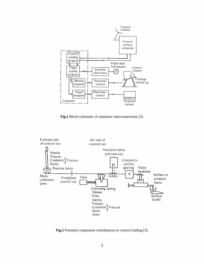
simulator such as the one in Fig.1.

The first ―ground based‖ flight simulator—Link Trainer—was built in the early 1920s by Edwin A. Link

[2]. It had a pneumatic motion platform driven by bellows, which provided pitch, roll, and yaw motion

cues. By 1969 hydraulic actuators had begun to provide motion cues in commercial flight simulators.

Shortly, the 6 degree of freedom (DOF) motion base—hydraulic driven Steward Platform—brought

simulators to their next generation. About the same time hydraulic actuators also began to replace older,

passive control feeling generators, such as mechanical springs, viscous dampers or electromechanical

brakes. Hydraulic control actuators used in flight simulators are low friction devices, controlled by

analog or digital computers to provide simulated motion and control dynamics. Fig.2 illustrates typical

components that contribute to the control feeling sensed by the pilot.

2

Fig.1 Block schematic of simulator interconnections [3].

Fig.2 Potential component contributions to control loading [3].

3

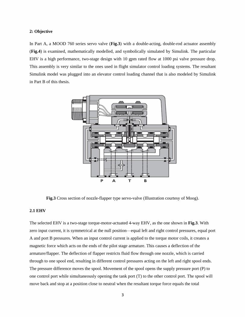
2: Objective

In Part A, a MOOD 760 series servo valve (Fig.3) with a double-acting, double-rod actuator assembly

(Fig.4) is examined, mathematically modelled, and symbolically simulated by Simulink. The particular

EHV is a high performance, two-stage design with 10 gpm rated flow at 1000 psi valve pressure drop.

This assembly is very similar to the ones used in flight simulator control loading systems. The resultant

Simulink model was plugged into an elevator control loading channel that is also modeled by Simulink

in Part B of this thesis.

Fig.3 Cross section of nozzle-flapper type servo-valve (Illustration courtesy of Moog).

2.1 EHV

The selected EHV is a two-stage torque-motor-actuated 4-way EHV, as the one shown in Fig.3. With

zero input current, it is symmetrical at the null position—equal left and right control pressures, equal port

A and port B pressures. When an input control current is applied to the torque motor coils, it creates a

magnetic force which acts on the ends of the pilot stage armature. This causes a deflection of the

armature/flapper. The deflection of flapper restricts fluid flow through one nozzle, which is carried

through to one spool end, resulting in different control pressures acting on the left and right spool ends.

The pressure difference moves the spool. Movement of the spool opens the supply pressure port (P) to

one control port while simultaneously opening the tank port (T) to the other control port. The spool will

move back and stop at a position close to neutral when the resultant torque force equals the total

4

restoring forces due to the feedback spring and the pressure difference between port A and port B. Then

the spool is held open in a state of equilibrium until the command signal changes to a new level. In

summary, the spool position is proportional to the input current with constant pressure drop across the

valve, and the flow to the load is proportional to the spool position [4].

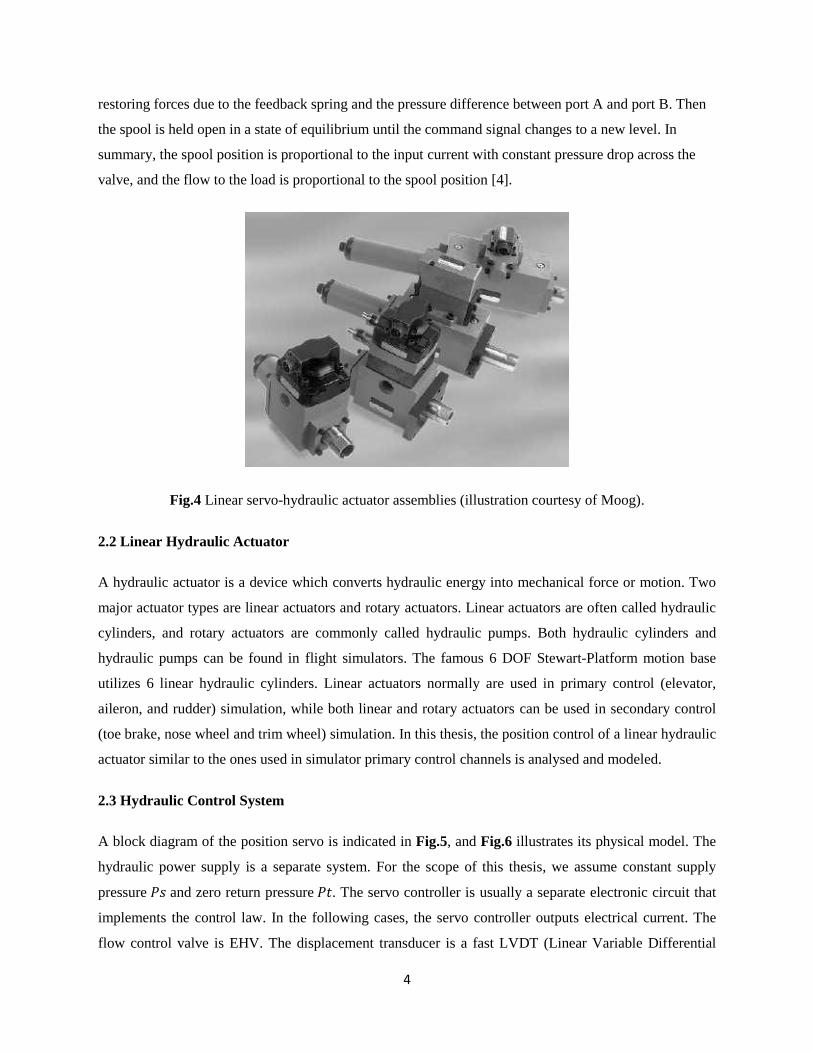
Fig.4 Linear servo-hydraulic actuator assemblies (illustration courtesy of Moog).

2.2 Linear Hydraulic Actuator

A hydraulic actuator is a device which converts hydraulic energy into mechanical force or motion. Two

major actuator types are linear actuators and rotary actuators. Linear actuators are often called hydraulic

cylinders, and rotary actuators are commonly called hydraulic pumps. Both hydraulic cylinders and

hydraulic pumps can be found in flight simulators. The famous 6 DOF Stewart-Platform motion base

utilizes 6 linear hydraulic cylinders. Linear actuators normally are used in primary control (elevator,

aileron, and rudder) simulation, while both linear and rotary actuators can be used in secondary control

(toe brake, nose wheel and trim wheel) simulation. In this thesis, the position control of a linear hydraulic

actuator similar to the ones used in simulator primary control channels is analysed and modeled.

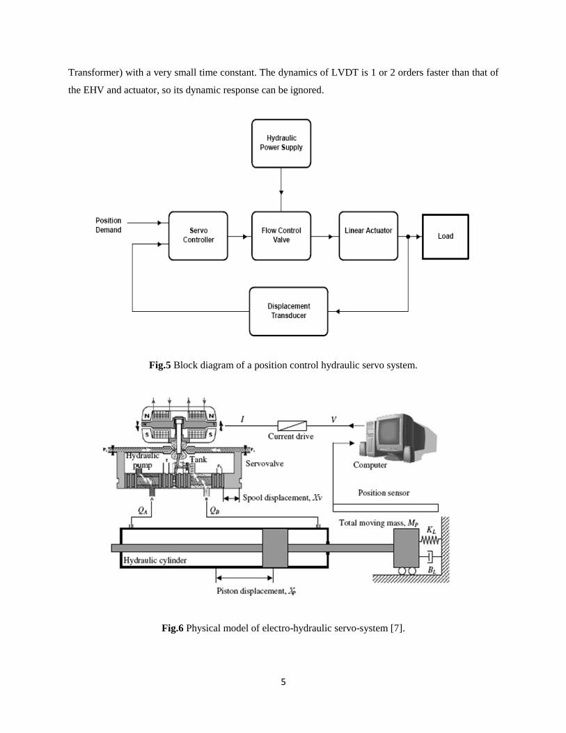
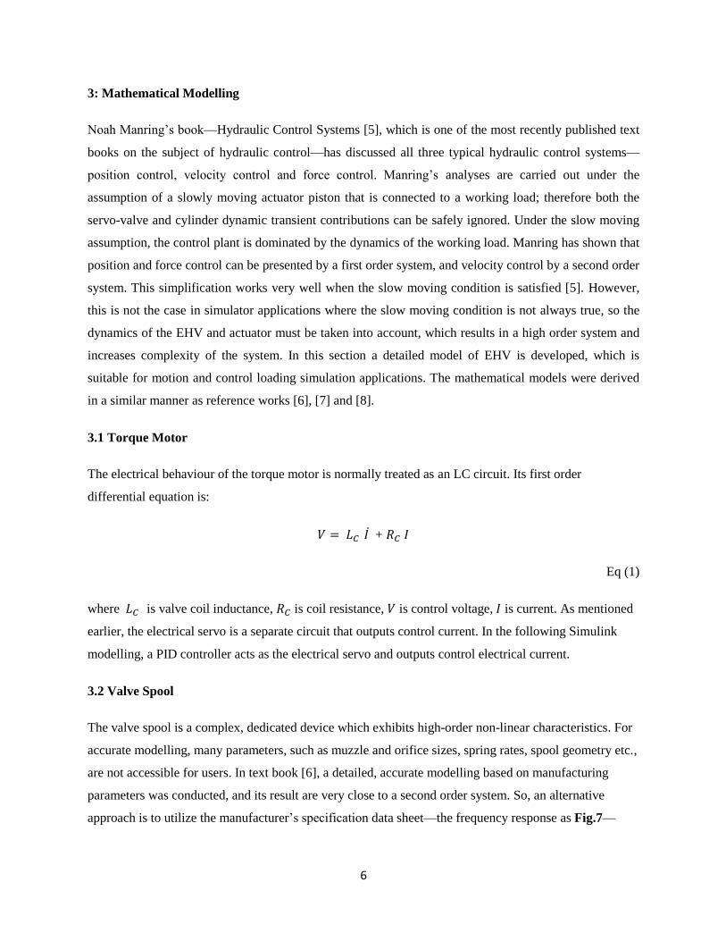
2.3 Hydraulic Control System

A block diagram of the position servo is indicated in Fig.5, and Fig.6 illustrates its physical model. The

hydraulic power supply is a separate system. For the scope of this thesis, we assume constant supply

pressure and zero return pressure . The servo controller is usually a separate electronic circuit that

implements the control law. In the following cases, the servo controller outputs electrical current. The

flow control valve is EHV. The displacement transducer is a fast LVDT (Linear Variable Differential

5

Transformer) with a very small time constant. The dynamics of LVDT is 1 or 2 orders faster than that of

the EHV and actuator, so its dynamic response can be ignored.

Fig.5 Block diagram of a position control hydraulic servo system.

Fig.6 Physical model of electro-hydraulic servo-system [7].

6

3: Mathematical Modelling

Noah Manring‘s book—Hydraulic Control Systems [5], which is one of the most recently published text

books on the subject of hydraulic control—has discussed all three typical hydraulic control systems—

position control, velocity control and force control. Manring‘s analyses are carried out under the

assumption of a slowly moving actuator piston that is connected to a working load; therefore both the

servo-valve and cylinder dynamic transient contributions can be safely ignored. Under the slow moving

assumption, the control plant is dominated by the dynamics of the working load. Manring has shown that

position and force control can be presented by a first order system, and velocity control by a second order

system. This simplification works very well when the slow moving condition is satisfied [5]. However,

this is not the case in simulator applications where the slow moving condition is not always true, so the

dynamics of the EHV and actuator must be taken into account, which results in a high order system and

increases complexity of the system. In this section a detailed model of EHV is developed, which is

suitable for motion and control loading simulation applications. The mathematical models were derived

in a similar manner as reference works [6], [7] and [8].

3.1 Torque Motor

The electrical behaviour of the torque motor is normally treated as an LC circuit. Its first order

differential equation is:

+

Eq (1)

where is valve coil inductance, is coil resistance, is control voltage, is current. As mentioned

earlier, the electrical servo is a separate circuit that outputs control current. In the following Simulink

modelling, a PID controller acts as the electrical servo and outputs control electrical current.

3.2 Valve Spool

The valve spool is a complex, dedicated device which exhibits high-order non-linear characteristics. For

accurate modelling, many parameters, such as muzzle and orifice sizes, spring rates, spool geometry etc.,

are not accessible for users. In text book [6], a detailed, accurate modelling based on manufacturing

parameters was conducted, and its result are very close to a second order system. So, an alternative

approach is to utilize the manufacturer‘s specification data sheet—the frequency response as Fig.7—

7

through which we can readily obtain the spool‘s natural frequency and damping ratio . In this case

=534 rad/s, =0.48.

Fig.7 Servo-valve frequency response curve (illustration courtesy of Moog) [4].

The corresponding second order differential equation is:

+ 2

+ =

Eq (2)

where is the servo-valve spool displacement, is the servo-valve spool natural frequency, is the

servo-valve spool damping ratio, = is the normalized input current, is the input current, and

is the saturation current for the torque motor.

3.3 Valve Flow-Pressure

The calculation of flow rate requires the classic orifice equation, which is developed based on the

Bernoilli equation and therefore is applicable for steady, incompressible, high-Reynolds-number flow.

The orifice equation is given by [10]

Q =

Eq (3)

where is the cross-sectional area of the orifice and is the discharge coefficient. When the geometry

is not exactly known, or when experimental results are not available, a sharp-edged orifice result of 0.62

8

is typically used for the discharge coefficient [10]. The significance of orifice is that it acts as the

fundamental building block in hydraulic control systems, as the P-N junction does in electro control

systems.

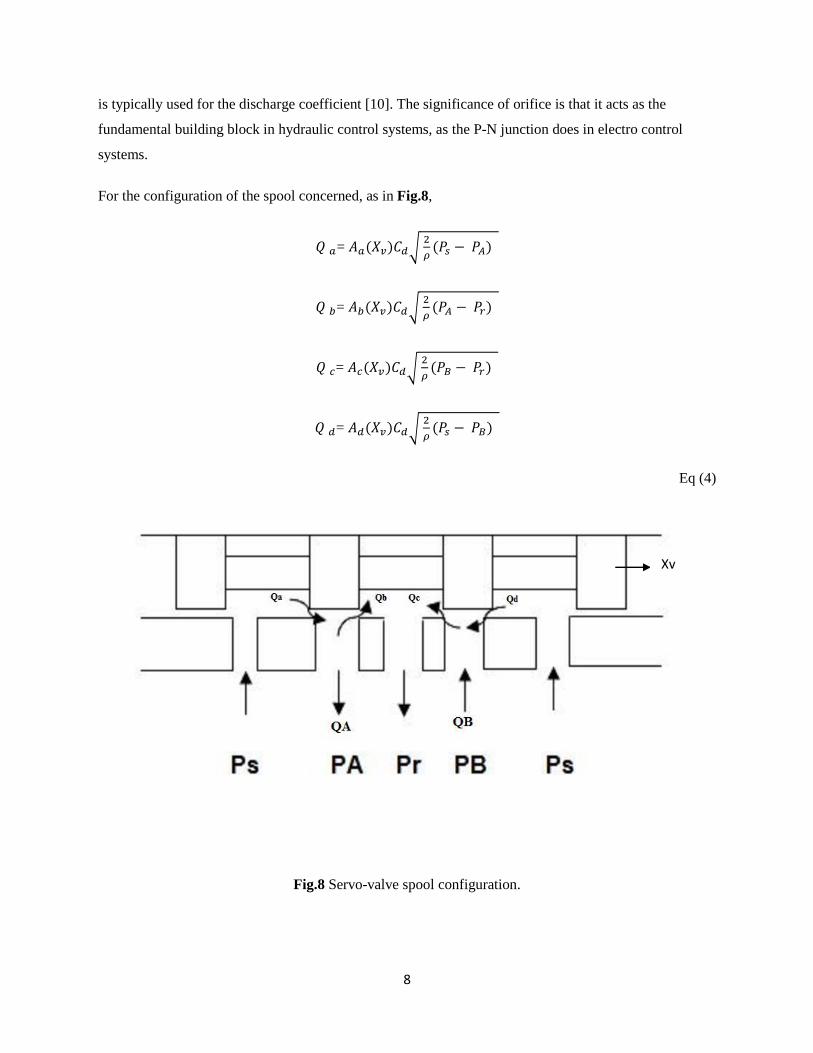
For the configuration of the spool concerned, as in Fig.8,

=

=

=

=

Eq (4)

Fig.8 Servo-valve spool configuration.

Xv

9

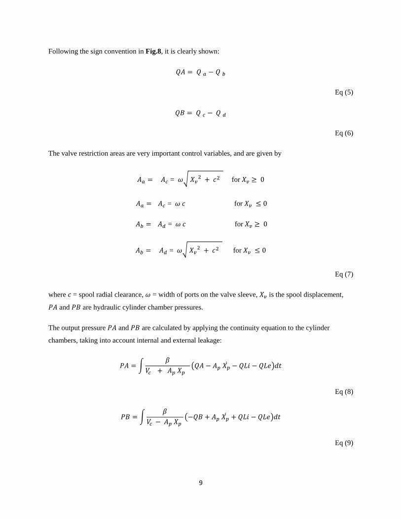
Following the sign convention in Fig.8, it is clearly shown:

Eq (5)

Eq (6)

The valve restriction areas are very important control variables, and are given by

= for

= for

= for

= for

Eq (7)

where = spool radial clearance, = width of ports on the valve sleeve, is the spool displacement,

and are hydraulic cylinder chamber pressures.

The output pressure and are calculated by applying the continuity equation to the cylinder

chambers, taking into account internal and external leakage:

Eq (8)

Eq (9)

10

where is the cylinder chamber volume in the null condition, is the piston displacement, the and

initial pressure is is the internal leakage, and is the external leakage.

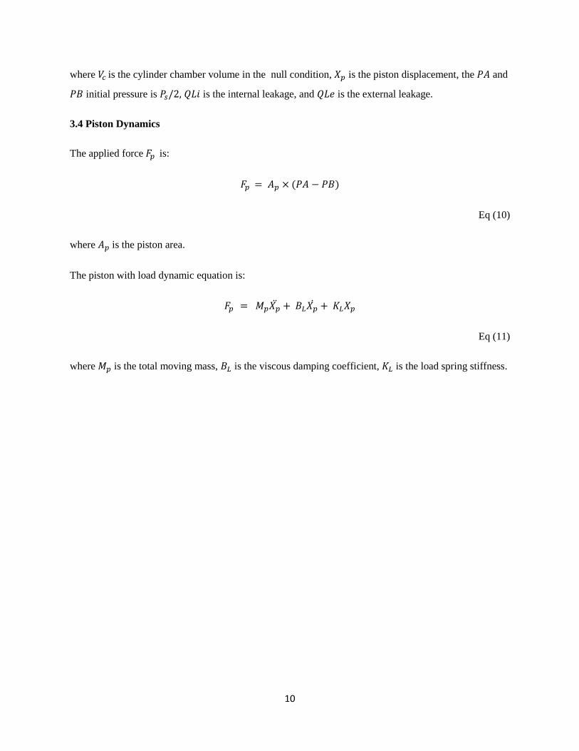
3.4 Piston Dynamics

The applied force is:

Eq (10)

where is the piston area.

The piston with load dynamic equation is:

Eq (11)

where is the total moving mass, is the viscous damping coefficient, is the load spring stiffness.

11

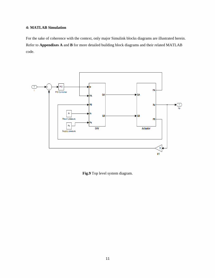
4: MATLAB Simulation

For the sake of coherence with the context, only major Simulink blocks diagrams are illustrated herein.

Refer to Appendixes A and B for more detailed building block diagrams and their related MATLAB

code.

Fig.9 Top level system diagram.

12

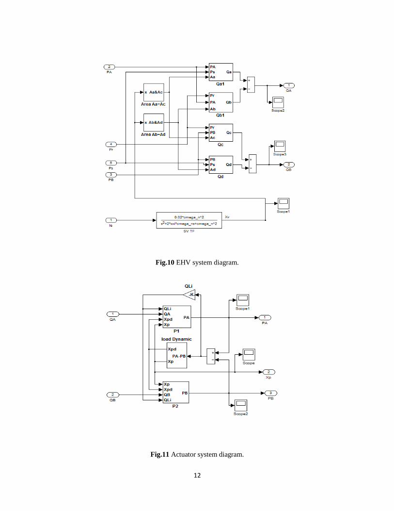
Fig.10 EHV system diagram.

Fig.11 Actuator system diagram.

13

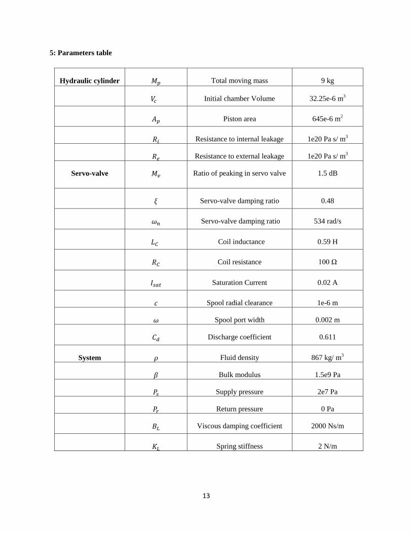
5: Parameters table

Hydraulic cylinder Total moving mass 9 kg

Initial chamber Volume 32.25e-6 m3

Piston area 645e-6 m2

Resistance to internal leakage 1e20 Pa s/ m3

Resistance to external leakage 1e20 Pa s/ m3

Servo-valve Ratio of peaking in servo valve 1.5 dB

Servo-valve damping ratio 0.48

Servo-valve damping ratio 534 rad/s

Coil inductance 0.59 H

Coil resistance 100 Ω

Saturation Current 0.02 A

Spool radial clearance 1e-6 m

Spool port width 0.002 m

Discharge coefficient 0.611

System Fluid density 867 kg/ m3

Bulk modulus 1.5e9 Pa

Supply pressure 2e7 Pa

Return pressure 0 Pa

Viscous damping coefficient 2000 Ns/m

Spring stiffness 2 N/m

14

6: Simulation Results and Discussion

6.1 EHV step response

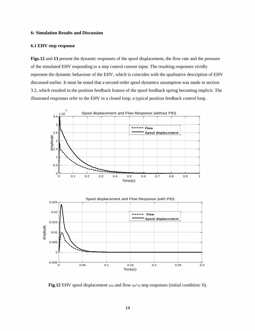
Figs.12 and 13 present the dynamic responses of the spool displacement, the flow rate and the pressure

of the simulated EHV responding to a step control current input. The resulting responses vividly

represent the dynamic behaviour of the EHV, which is coincides with the qualitative description of EHV

discussed earlier. It must be noted that a second order spool dynamics assumption was made in section

3.2, which resulted in the position feedback feature of the spool feedback spring becoming implicit. The

illustrated responses refer to the EHV in a closed loop; a typical position feedback control loop.

Fig.12 EHV spool displacement (m) and flow (m3/s) step responses (initial condition: 0).

0 0.1 0.2 0.3 0.4 0.5 0.6 0.7 0.8 0.9 10

0.5

1

1.5

2

2.5

3

3.5x 10

-3

Time(s)

Am

plit

ude

Spool displacement and Flow Response (without PID)

Flow

Spool displacement

0 0.05 0.1 0.15 0.2 0.25 0.3-0.005

0

0.005

0.01

0.015

0.02

0.025

Time(s)

Am

pltu

de

Spool displacement and Flow Response (with PID)

Flow

Spool displacement

15

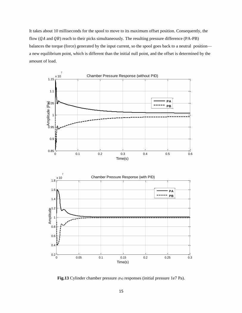
It takes about 10 milliseconds for the spool to move to its maximum offset position. Consequently, the

flow ( and ) reach to their picks simultaneously. The resulting pressure difference (PA-PB)

balances the torque (force) generated by the input current, so the spool goes back to a neutral position—

a new equilibrium point, which is different than the initial null point, and the offset is determined by the

amount of load.

Fig.13 Cylinder chamber pressure (Pa) responses (initial pressure 1e7 Pa).

0 0.1 0.2 0.3 0.4 0.5 0.60.85

0.9

0.95

1

1.05

1.1

1.15x 10

7

Time(s)

Am

plit

ude (

Pa)

Chamber Pressure Response (without PID)

PA

PB

0 0.05 0.1 0.15 0.2 0.25 0.30.2

0.4

0.6

0.8

1

1.2

1.4

1.6

1.8x 10

7

Time(s)

Am

plit

ude

Chamber Pressure Response (with PID)

PA

PB

16

Comparing different control implementations between the simple feedback and the tuned PID controller,

it can be seen that the response of the tuned PID controller is much faster than that of the unturned

simple feedback control. However, a faster response requires higher mechanical capability; in this case it

requires a bigger maximum allowable spool displacement and adequate availability of flow supply. This

can be realized in both Figs. 12 and 13. In industry practice, the choosing of EHV and a control scheme

is a trade-off between cost and performance.

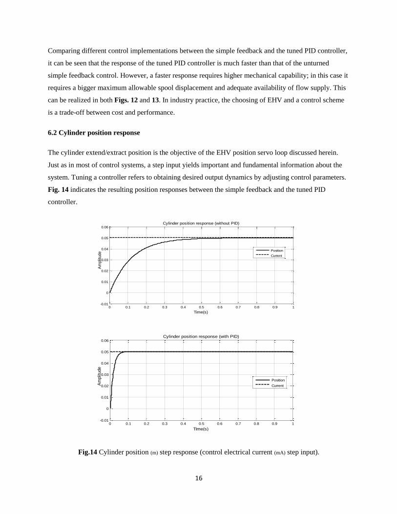
6.2 Cylinder position response

The cylinder extend/extract position is the objective of the EHV position servo loop discussed herein.

Just as in most of control systems, a step input yields important and fundamental information about the

system. Tuning a controller refers to obtaining desired output dynamics by adjusting control parameters.

Fig. 14 indicates the resulting position responses between the simple feedback and the tuned PID

controller.

Fig.14 Cylinder position (m) step response (control electrical current (mA) step input).

0 0.1 0.2 0.3 0.4 0.5 0.6 0.7 0.8 0.9 1-0.01

0

0.01

0.02

0.03

0.04

0.05

0.06

Time(s)

Am

plit

ude

Cylinder position response (without PID)

Position

Current

0 0.1 0.2 0.3 0.4 0.5 0.6 0.7 0.8 0.9 1-0.01

0

0.01

0.02

0.03

0.04

0.05

0.06

TIme(s)

Am

plit

ude

Cylinder position response (with PID)

Position

Current

17

The response of the simple feedback has longer and , obviously not the desired response. The

tuned PID controller has a satisfactory response. The PDI gain terms can be tuned according to the

Ziegler-Nichols rule. In the turning process, it was noticed that an adequate response could be obtained

by tuning the proportional gain alone. The simple feedback controller can obtain a good shape of the

position response curve by increasing the feedback gain alone. However, getting the desired output

response is not the only design objective. For example, increasing feedback gain will reduce the general

gain of the system for a given input current, and so the electric control current must be increased to get

the required position output, which means reducing the stability margin and usable working range of the

EHV. As in any product design, the controller design is an iterative process to optimize the balance

between performance, cost, system robustness and maintainability. In the case of motion and control

loading controller design, the ease of tuning the controller should also be taken into account.

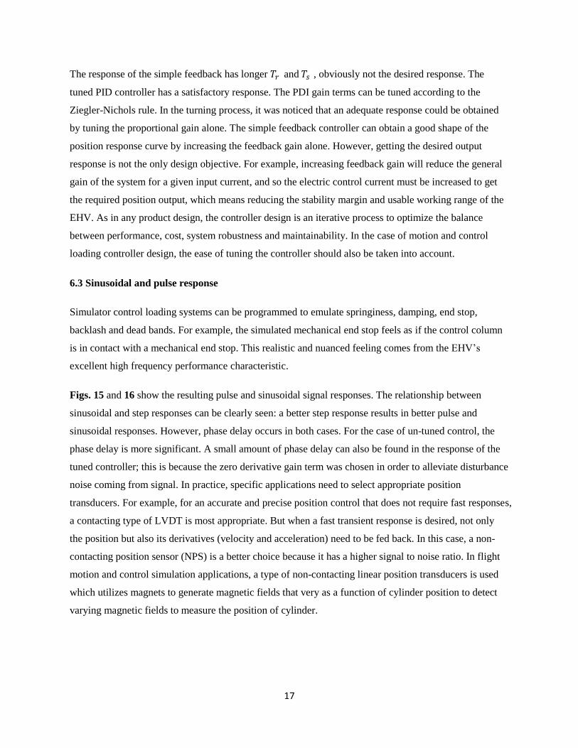
6.3 Sinusoidal and pulse response

Simulator control loading systems can be programmed to emulate springiness, damping, end stop,

backlash and dead bands. For example, the simulated mechanical end stop feels as if the control column

is in contact with a mechanical end stop. This realistic and nuanced feeling comes from the EHV‘s

excellent high frequency performance characteristic.

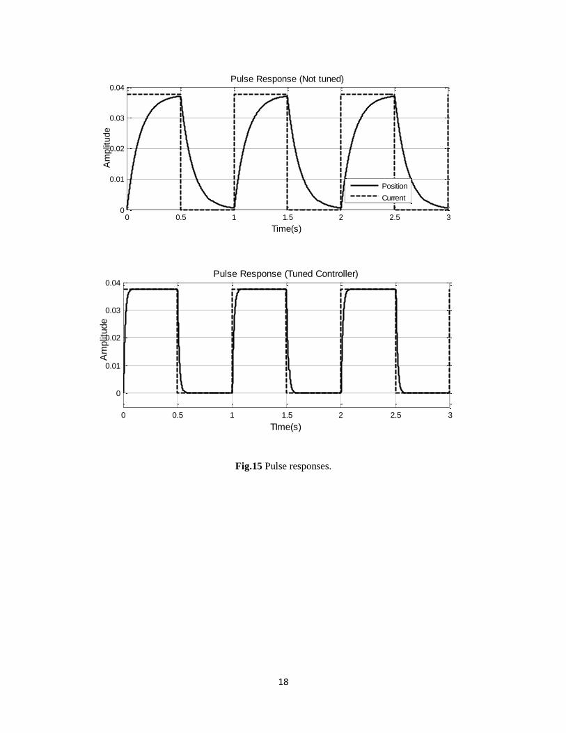
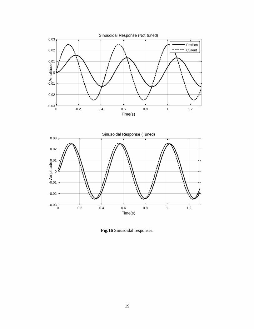
Figs. 15 and 16 show the resulting pulse and sinusoidal signal responses. The relationship between

sinusoidal and step responses can be clearly seen: a better step response results in better pulse and

sinusoidal responses. However, phase delay occurs in both cases. For the case of un-tuned control, the

phase delay is more significant. A small amount of phase delay can also be found in the response of the

tuned controller; this is because the zero derivative gain term was chosen in order to alleviate disturbance

noise coming from signal. In practice, specific applications need to select appropriate position

transducers. For example, for an accurate and precise position control that does not require fast responses,

a contacting type of LVDT is most appropriate. But when a fast transient response is desired, not only

the position but also its derivatives (velocity and acceleration) need to be fed back. In this case, a non-

contacting position sensor (NPS) is a better choice because it has a higher signal to noise ratio. In flight

motion and control simulation applications, a type of non-contacting linear position transducers is used

which utilizes magnets to generate magnetic fields that very as a function of cylinder position to detect

varying magnetic fields to measure the position of cylinder.

18

Fig.15 Pulse responses.

0 0.5 1 1.5 2 2.5 30

0.01

0.02

0.03

0.04

Time(s)

Am

plit

ude

Pulse Response (Not tuned)

Position

Current

0 0.5 1 1.5 2 2.5 3

0

0.01

0.02

0.03

0.04

TIme(s)

Am

plit

ude

Pulse Response (Tuned Controller)

19

Fig.16 Sinusoidal responses.

0 0.2 0.4 0.6 0.8 1 1.2-0.03

-0.02

-0.01

0

0.01

0.02

0.03

Time(s)

Am

plit

ude

Sinusoidal Response (Not tuned)

Position

Current

0 0.2 0.4 0.6 0.8 1 1.2-0.03

-0.02

-0.01

0

0.01

0.02

0.03

Time(s)

Am

plit

ude

Sinusoidal Response (Tuned)

20

7: Summary of Part A

An EHV Simulink model has been established based on the mechanical parameters of the EHV. This

model can serve as a platform to investigate the dynamics of EHVs, which will be used for the flight

simulators under study in Part B. It is noted that the presented model can be further refined in future

research, for example, by taking into account for friction. Although a hydraulic linear cylinder is known

as a low friction device; friction could considerably influences the high-end performance. Also as

described in section 3.2, the EHV spool dynamics was derived approximately from the resulting

characteristic response curves of the selected EHV. Obtaining of the actual manufacturing data of the

EHV will improve the fidelity of the EHV simulation.

A position servo control has been constructed using the resultant EHV Simulink model and the linear

hydraulic double-ended cylinder Simulink model. The construction of the position servo and its control

parameter tuning process revealed that the choosing of an EHV that has certain specifications to match a

particular control scheme is a trade-off between the cost of EHV and the servo control performance

required. The design is always an iterative and optimizing process.

We now move on to Part B, in which we consider aircraft motion and control loading simulation, a

practical application of electro-hydraulic servo-valve and hydraulic control servo.

21

Part B Simulator Motion and Control loading

8: Introduction

Part B of this thesis is about motion and control loading systems of flight simulators. Simulators have

utilized electro-hydraulic servo-valves as a means of actuation of motion and control loading simulation

for more than half a century. The use of EHV in simulators is an important application of EHV.

The design and development of modern aircraft makes extensive use of flight simulation. There are three

major categories of simulators [3]: in-flight simulators, ground-based researching simulators and pilot

training simulators. This thesis is concerned with only the third one–pilot training simulators. There is a

vast range of problems open to investigation on simulators, but the essential feature of all such

investigations is to introduce the pilot into a closed loop control situation. One of the most important

simulation objectives is to simulate the static and dynamic behaviour of aircraft in real flight situations. It

should be noted that it is impossible and not feasible to simulate the complete range of the flight dynamic

profile of real aircraft. Hence we focus on certain segments of the static and dynamic profile that are

needed for pilots‘ training. Currently, the simulation industry is able to provide pilots with simulators

that can comply with all regulatory specified requirements. The scope of Part B is to examine simulator

motion and control loading systems, and the goal is to fully understand the simulation of aircraft motion

and control loading.

In the following sections, motion and control loading simulation will be examined in detail. First, real

aircraft motion and control are introduced, followed by simulation algorithms and mathematical models.

An elevator control loading channel is represented in state space and also symbolically modelled using

the EHV model devolved in Part A. The focus is on control scheme implementations. Regulatory tests

and evaluation are reviewed as the final objective of the simulation. Also, industry examples of digital

hydraulic motion and control loading, and the latest electric motion and control loading systems are

introduced.

22

9: Motion simulation

9.1 Aircraft motion equation

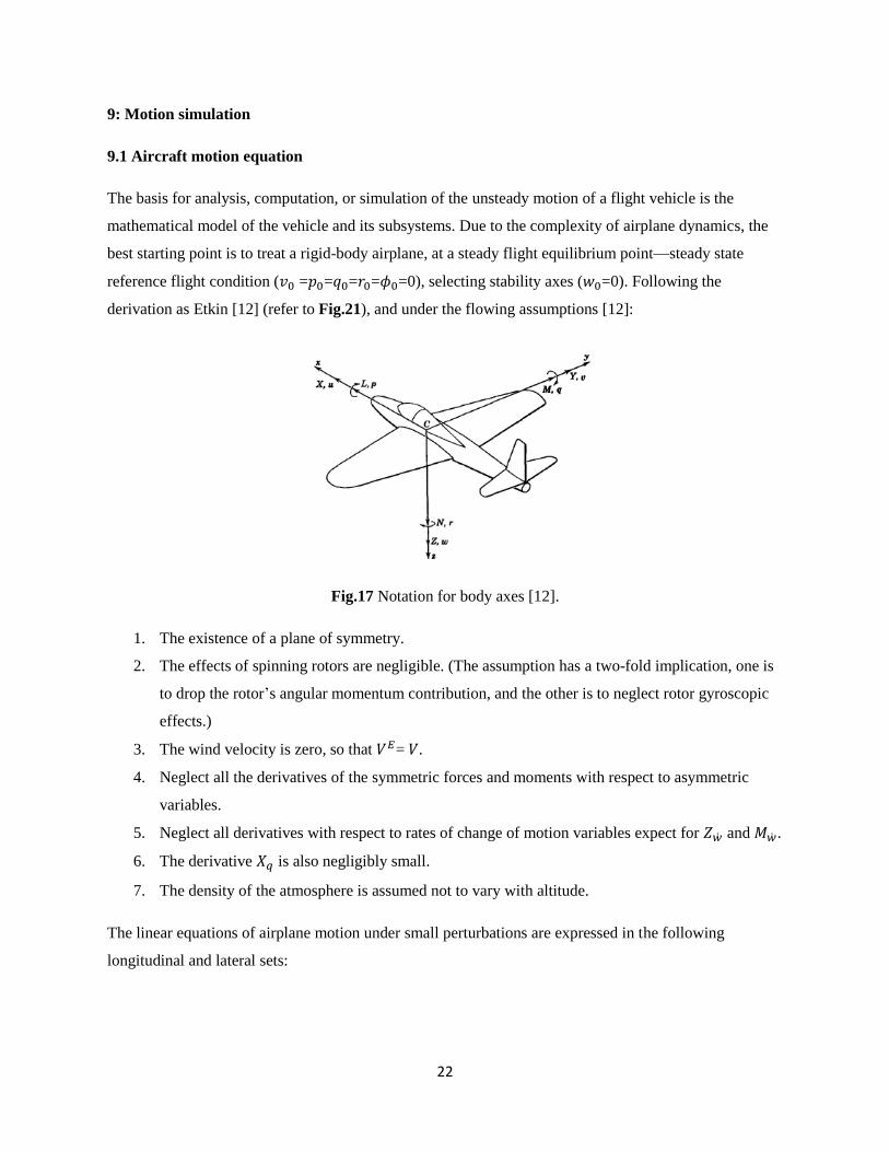
The basis for analysis, computation, or simulation of the unsteady motion of a flight vehicle is the

mathematical model of the vehicle and its subsystems. Due to the complexity of airplane dynamics, the

best starting point is to treat a rigid-body airplane, at a steady flight equilibrium point—steady state

reference flight condition ( = = = = =0), selecting stability axes ( =0). Following the

derivation as Etkin [12] (refer to Fig.21), and under the flowing assumptions [12]:

Fig.17 Notation for body axes [12].

1. The existence of a plane of symmetry.

2. The effects of spinning rotors are negligible. (The assumption has a two-fold implication, one is

to drop the rotor‘s angular momentum contribution, and the other is to neglect rotor gyroscopic

effects.)

3. The wind velocity is zero, so that = .

4. Neglect all the derivatives of the symmetric forces and moments with respect to asymmetric

variables.

5. Neglect all derivatives with respect to rates of change of motion variables expect for and .

6. The derivative is also negligibly small.

7. The density of the atmosphere is assumed not to vary with altitude.

The linear equations of airplane motion under small perturbations are expressed in the following

longitudinal and lateral sets:

23

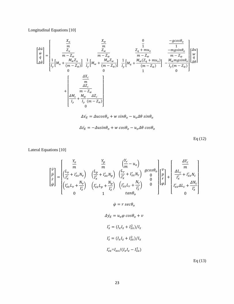
Longitudinal Equations [10]

Eq (12)

Lateral Equations [10]

=

Eq (13)

24

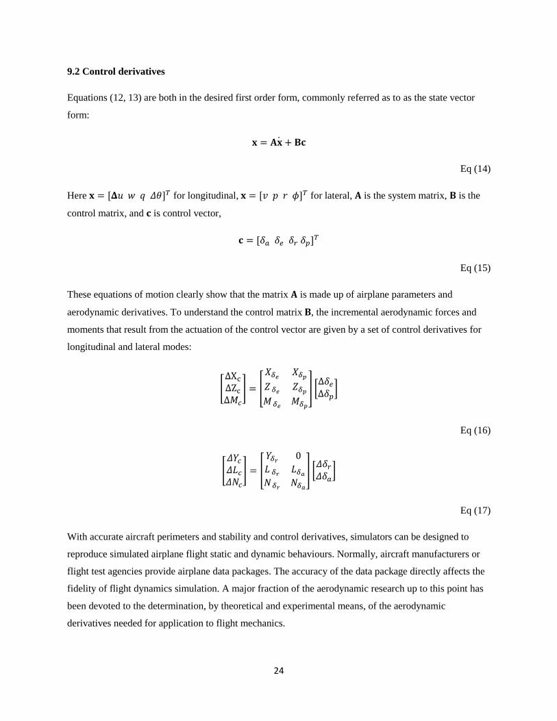
9.2 Control derivatives

Equations (12, 13) are both in the desired first order form, commonly referred as to as the state vector

form:

Eq (14)

Here for longitudinal, for lateral, is the system matrix, is the

control matrix, and is control vector,

Eq (15)

These equations of motion clearly show that the matrix is made up of airplane parameters and

aerodynamic derivatives. To understand the control matrix , the incremental aerodynamic forces and

moments that result from the actuation of the control vector are given by a set of control derivatives for

longitudinal and lateral modes:

Eq (16)

Eq (17)

With accurate aircraft perimeters and stability and control derivatives, simulators can be designed to

reproduce simulated airplane flight static and dynamic behaviours. Normally, aircraft manufacturers or

flight test agencies provide airplane data packages. The accuracy of the data package directly affects the

fidelity of flight dynamics simulation. A major fraction of the aerodynamic research up to this point has

been devoted to the determination, by theoretical and experimental means, of the aerodynamic

derivatives needed for application to flight mechanics.

25

Simulators can be made before and/or after airplanes have been manufactured. Practically, at an

airplane‘s detailed design stage, the simulated airplane simulator can be a test tool for airframe and

control system design, providing a means to evaluate alternative design strategies [3]; this application of

simulator in turn demands more thorough and accurate aircraft simulation of the simulator.

Strictly speaking, aerodynamic forces and moments are functions of state variables. Forces and moments

may need to be expressed as functions of one or more of the following: [3]

Angle of attack

Control deflections

Speed/Mach number

Rotation rate

Height

Centre gravity position

Ground proximity

Geometry (e.g., flap setting, wing sweep, leading gear)

Consequently, the aerodynamic and control derivatives are not constants, and not even linear functions of

those factors. For dealing with nonlinearity, curve fitting techniques such as polynomial curve fitting and

table look-up techniques are used.

Eq (18)

Eq (19)

The choosing of 1st order or second2

nd order depends on the nature of the derivative. For example, the

pitching moment coefficient as a function of angle of attack , the derivative plays a major role

on an airplane‘s longitudinal stability. So, the second order polynomial Eq (19) brings more fidelity in

this case.

In cases where and , are functions of the angle of attack, they are also functions of flap angle and

Mach number, so that , , are expressed as , where may be flap angle or Mach number.

Normally the data of and at specific flap angles are given, for instance. For flap angles between

the defined values, a technique is required to interpolate the appropriate valves of the dependent

26

coefficients , and . This often refers to ‗table look-up.‘ Table look-up basically refers to linear

interpolation between adjacent coordinate pairs. A significant amount of aero data look-up tables are

used in simulation software models, and especially in aerodynamic flight modules. In some special cases,

high order interpolation techniques, such as cubic spines, are used to maintain continuity of the data

slope [3].

9.3 History of simulator motion

For ground-based pilot training simulators, in addition to replicating the functionality of instrumentation

and navigation aids at the pilots‘ point of view, all the cues that pilots perceive in a real aircraft, such as

visual, sound, control feeling and motion sense, are simulated with considerable fidelity. Of these,

motion cue simulation is the most difficult because of the physical restrictions of the simulator‘s ground-

based structure.

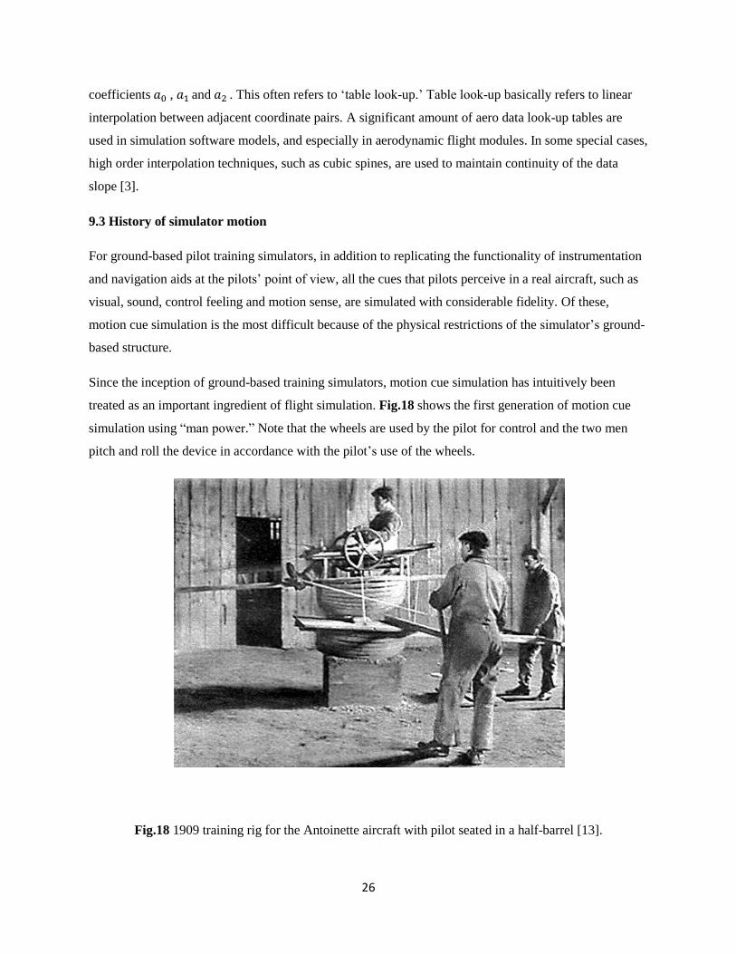
Since the inception of ground-based training simulators, motion cue simulation has intuitively been

treated as an important ingredient of flight simulation. Fig.18 shows the first generation of motion cue

simulation using ―man power.‖ Note that the wheels are used by the pilot for control and the two men

pitch and roll the device in accordance with the pilot‘s use of the wheels.

Fig.18 1909 training rig for the Antoinette aircraft with pilot seated in a half-barrel [13].

27

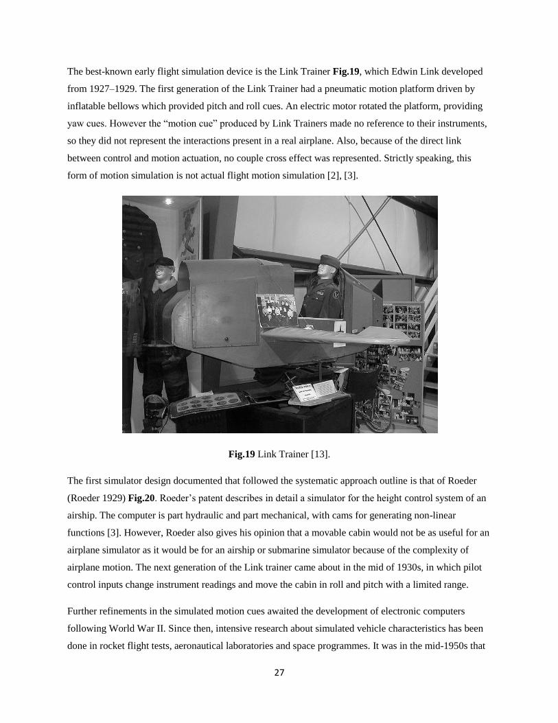
The best-known early flight simulation device is the Link Trainer Fig.19, which Edwin Link developed

from 1927–1929. The first generation of the Link Trainer had a pneumatic motion platform driven by

inflatable bellows which provided pitch and roll cues. An electric motor rotated the platform, providing

yaw cues. However the ―motion cue‖ produced by Link Trainers made no reference to their instruments,

so they did not represent the interactions present in a real airplane. Also, because of the direct link

between control and motion actuation, no couple cross effect was represented. Strictly speaking, this

form of motion simulation is not actual flight motion simulation [2], [3].

Fig.19 Link Trainer [13].

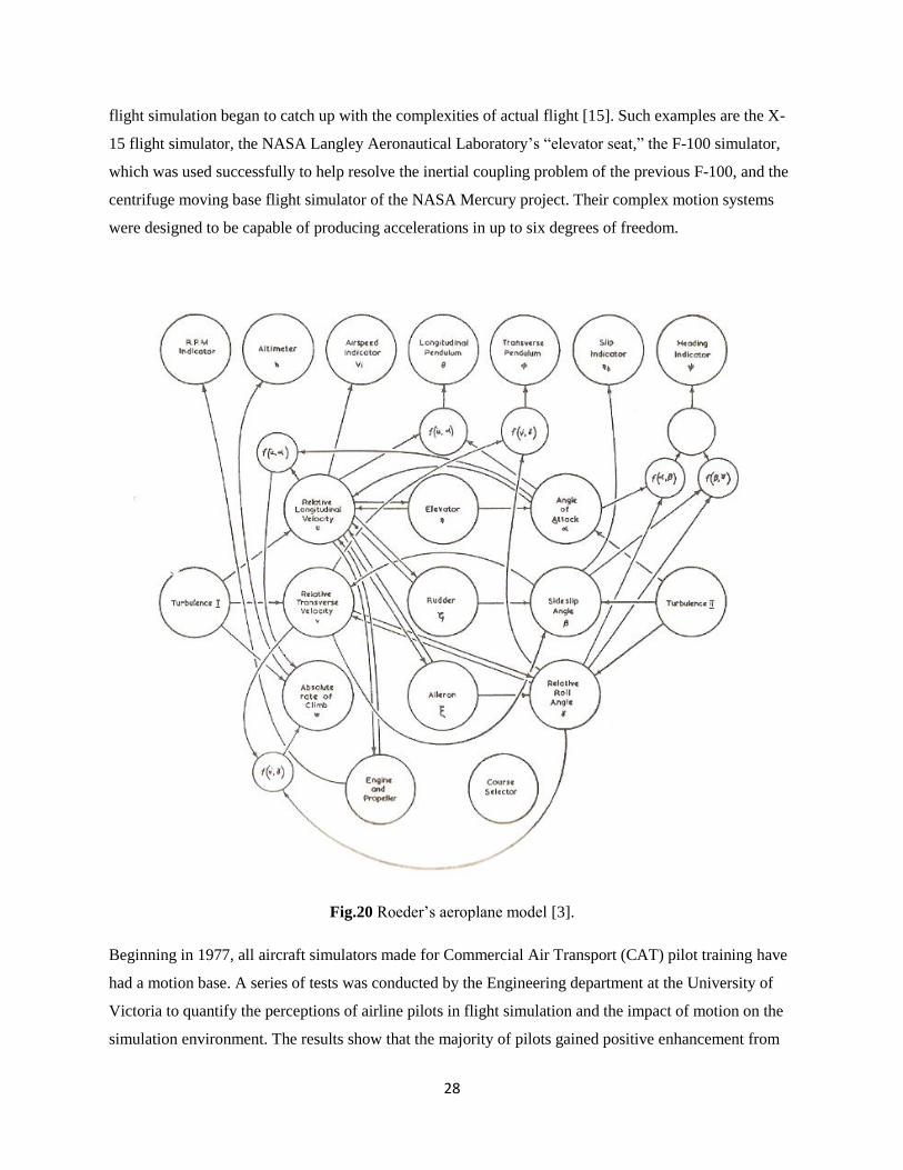
The first simulator design documented that followed the systematic approach outline is that of Roeder

(Roeder 1929) Fig.20. Roeder‘s patent describes in detail a simulator for the height control system of an

airship. The computer is part hydraulic and part mechanical, with cams for generating non-linear

functions [3]. However, Roeder also gives his opinion that a movable cabin would not be as useful for an

airplane simulator as it would be for an airship or submarine simulator because of the complexity of

airplane motion. The next generation of the Link trainer came about in the mid of 1930s, in which pilot

control inputs change instrument readings and move the cabin in roll and pitch with a limited range.

Further refinements in the simulated motion cues awaited the development of electronic computers

following World War II. Since then, intensive research about simulated vehicle characteristics has been

done in rocket flight tests, aeronautical laboratories and space programmes. It was in the mid-1950s that

28

flight simulation began to catch up with the complexities of actual flight [15]. Such examples are the X-

15 flight simulator, the NASA Langley Aeronautical Laboratory‘s ―elevator seat,‖ the F-100 simulator,

which was used successfully to help resolve the inertial coupling problem of the previous F-100, and the

centrifuge moving base flight simulator of the NASA Mercury project. Their complex motion systems

were designed to be capable of producing accelerations in up to six degrees of freedom.

Fig.20 Roeder‘s aeroplane model [3].

Beginning in 1977, all aircraft simulators made for Commercial Air Transport (CAT) pilot training have

had a motion base. A series of tests was conducted by the Engineering department at the University of

Victoria to quantify the perceptions of airline pilots in flight simulation and the impact of motion on the

simulation environment. The results show that the majority of pilots gained positive enhancement from

29

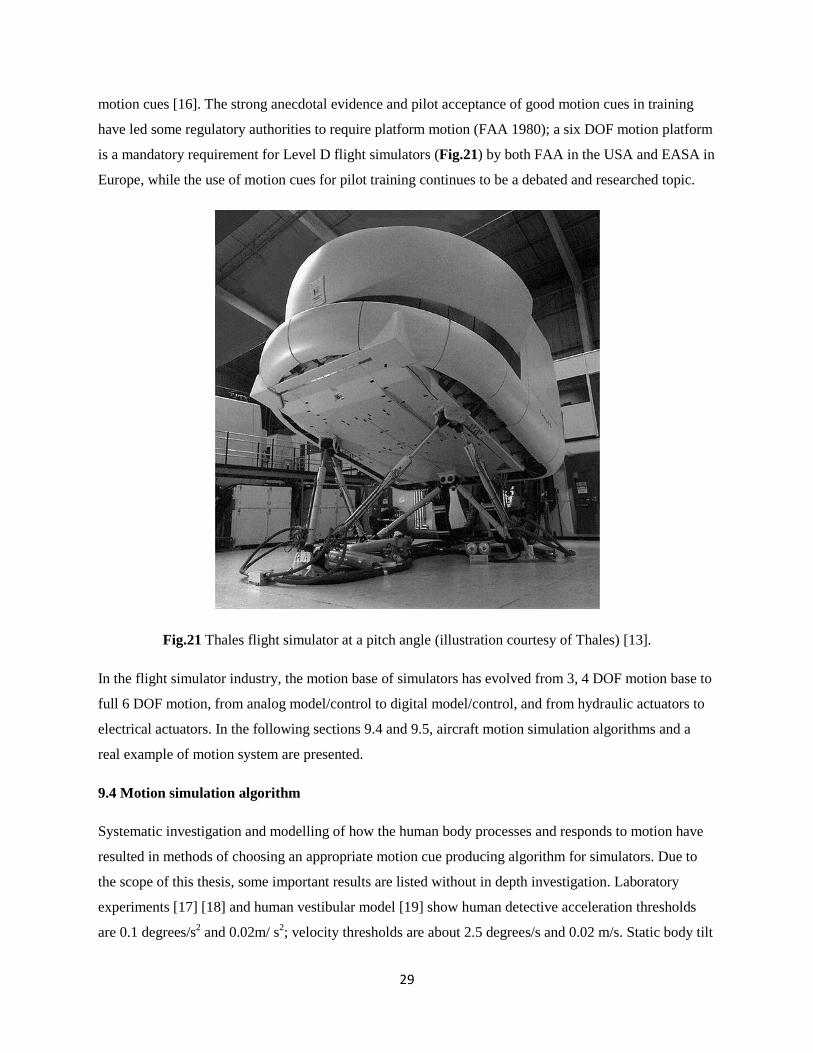
motion cues [16]. The strong anecdotal evidence and pilot acceptance of good motion cues in training

have led some regulatory authorities to require platform motion (FAA 1980); a six DOF motion platform

is a mandatory requirement for Level D flight simulators (Fig.21) by both FAA in the USA and EASA in

Europe, while the use of motion cues for pilot training continues to be a debated and researched topic.

Fig.21 Thales flight simulator at a pitch angle (illustration courtesy of Thales) [13].

In the flight simulator industry, the motion base of simulators has evolved from 3, 4 DOF motion base to

full 6 DOF motion, from analog model/control to digital model/control, and from hydraulic actuators to

electrical actuators. In the following sections 9.4 and 9.5, aircraft motion simulation algorithms and a

real example of motion system are presented.

9.4 Motion simulation algorithm

Systematic investigation and modelling of how the human body processes and responds to motion have

resulted in methods of choosing an appropriate motion cue producing algorithm for simulators. Due to

the scope of this thesis, some important results are listed without in depth investigation. Laboratory

experiments [17] [18] and human vestibular model [19] show human detective acceleration thresholds

are 0.1 degrees/s2 and 0.02m/ s

2; velocity thresholds are about 2.5 degrees/s and 0.02 m/s. Static body tilt

30

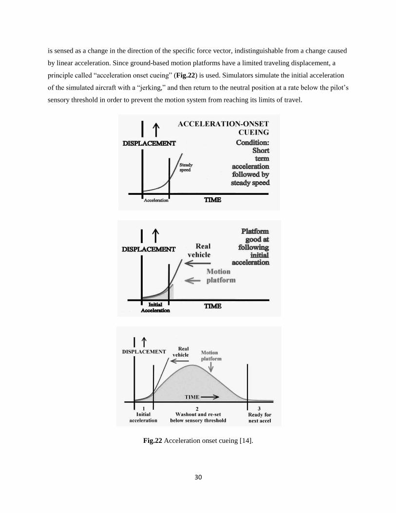
is sensed as a change in the direction of the specific force vector, indistinguishable from a change caused

by linear acceleration. Since ground-based motion platforms have a limited traveling displacement, a

principle called ―acceleration onset cueing‖ (Fig.22) is used. Simulators simulate the initial acceleration

of the simulated aircraft with a ―jerking,‖ and then return to the neutral position at a rate below the pilot‘s

sensory threshold in order to prevent the motion system from reaching its limits of travel.

Fig.22 Acceleration onset cueing [14].

31

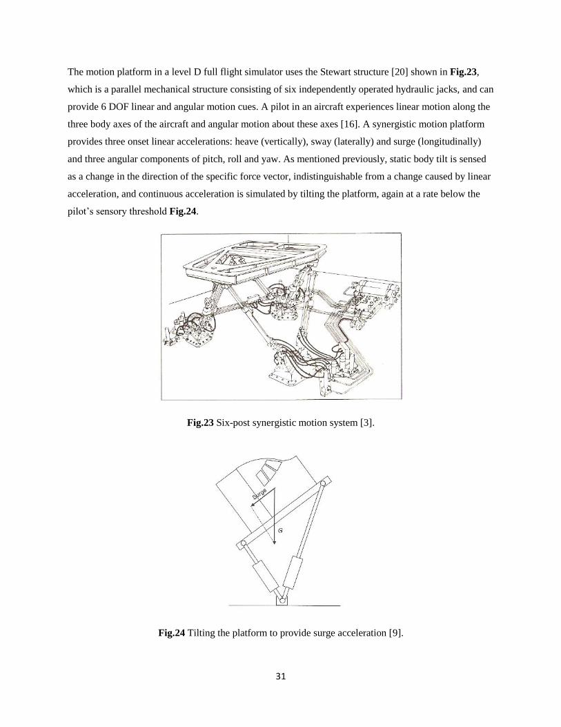
The motion platform in a level D full flight simulator uses the Stewart structure [20] shown in Fig.23,

which is a parallel mechanical structure consisting of six independently operated hydraulic jacks, and can

provide 6 DOF linear and angular motion cues. A pilot in an aircraft experiences linear motion along the

three body axes of the aircraft and angular motion about these axes [16]. A synergistic motion platform

provides three onset linear accelerations: heave (vertically), sway (laterally) and surge (longitudinally)

and three angular components of pitch, roll and yaw. As mentioned previously, static body tilt is sensed

as a change in the direction of the specific force vector, indistinguishable from a change caused by linear

acceleration, and continuous acceleration is simulated by tilting the platform, again at a rate below the

pilot‘s sensory threshold Fig.24.

Fig.23 Six-post synergistic motion system [3].

Fig.24 Tilting the platform to provide surge acceleration [9].

32

Several different manufacturers have designed and manufactured their own kinds of motion systems

based on the Steward platform, with different cylinder diameters and lengths and different servo control

implementations. The first generation was an analog control 6-DOF motion base. A digital motion

system is functionally identical to the analog motion system but is realized in a digital format. The

benefit of digital over analog is commonly realized as that of any other production. Improvements of the

digital motion system over analog motion base are its user-friendly interface, the ease of motion cue

tuning and maintainability.

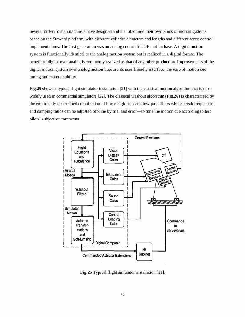
Fig.25 shows a typical flight simulator installation [21] with the classical motion algorithm that is most

widely used in commercial simulators [22]. The classical washout algorithm (Fig.26) is characterized by

the empirically determined combination of linear high-pass and low-pass filters whose break frequencies

and damping ratios can be adjusted off-line by trial and error—to tune the motion cue according to test

pilots‘ subjective comments.

Fig.25 Typical flight simulator installation [21].

33

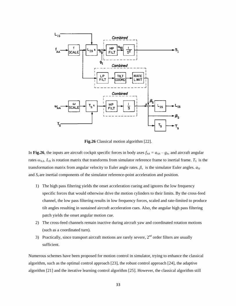
Fig.26 Classical motion algorithm [22].

In Fig.26, the inputs are aircraft cockpit specific forces in body axes fAA = aAA – gA, and aircraft angular

rates ωAA. LIS is rotation matrix that transforms from simulator reference frame to inertial frame. TS is the

transformation matrix from angular velocity to Euler angle rates. βs is the simulator Euler angles. aSI

and SI are inertial components of the simulator reference-point acceleration and position.

1) The high pass filtering yields the onset acceleration cueing and ignores the low frequency

specific forces that would otherwise drive the motion cylinders to their limits. By the cross-feed

channel, the low pass filtering results in low frequency forces, scaled and rate-limited to produce

tilt angles resulting in sustained aircraft acceleration cues. Also, the angular high pass filtering

patch yields the onset angular motion cue.

2) The cross-feed channels remain inactive during aircraft yaw and coordinated rotation motions

(such as a coordinated turn).

3) Practically, since transport aircraft motions are rarely severe, 2nd

order filters are usually

sufficient.

Numerous schemes have been proposed for motion control in simulator, trying to enhance the classical

algorithm, such as the optimal control approach [23], the robust control approach [24], the adaptive

algorithm [21] and the iterative learning control algorithm [25]. However, the classical algorithm still

34

dominates simulator manufacturing in the industry because 1) it is mathematically and computationally

simple, and hence computationally cheap, and 2) it is relatively transparent to the designer, and therefore

pilots‘ complaints can often be easily rectified [22].

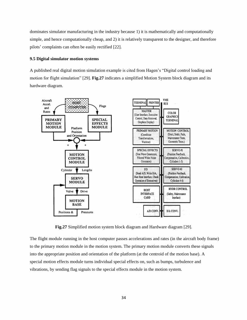
9.5 Digital simulator motion systems

A published real digital motion simulation example is cited from Hagen‘s ―Digital control loading and

motion for flight simulation‖ [29]. Fig.27 indicates a simplified Motion System block diagram and its

hardware diagram.

Fig.27 Simplified motion system block diagram and Hardware diagram [29].

The flight module running in the host computer passes accelerations and rates (in the aircraft body frame)

to the primary motion module in the motion system. The primary motion module converts these signals

into the appropriate position and orientation of the platform (at the centroid of the motion base). A

special motion effects module turns individual special effects on, such as bumps, turbulence and

vibrations, by sending flag signals to the special effects module in the motion system.

35

The hardware diagram demonstrates the computer structure of the motion system that uses a number of

processors running in parallel based on the VME bus. The iteration rate reaches up to the order of KHz;

control loops can be run smoothly in real time. There are six separated executives running on six cards:

primary motion, special effects, motion control, servo #1, servo #2 and I/O. The master card acts as

master executive of the system. It also runs the analysis and design programs—DIGITAL, which is used

for designing and turning the motion system servo.

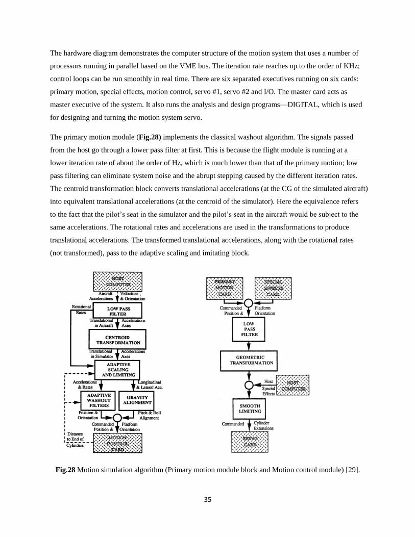
The primary motion module (Fig.28) implements the classical washout algorithm. The signals passed

from the host go through a lower pass filter at first. This is because the flight module is running at a

lower iteration rate of about the order of Hz, which is much lower than that of the primary motion; low

pass filtering can eliminate system noise and the abrupt stepping caused by the different iteration rates.

The centroid transformation block converts translational accelerations (at the CG of the simulated aircraft)

into equivalent translational accelerations (at the centroid of the simulator). Here the equivalence refers

to the fact that the pilot‘s seat in the simulator and the pilot‘s seat in the aircraft would be subject to the

same accelerations. The rotational rates and accelerations are used in the transformations to produce

translational accelerations. The transformed translational accelerations, along with the rotational rates

(not transformed), pass to the adaptive scaling and imitating block.

Fig.28 Motion simulation algorithm (Primary motion module block and Motion control module) [29].

36

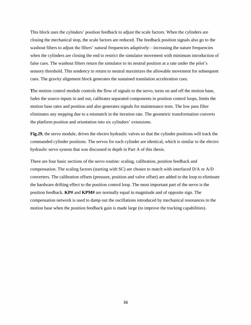
This block uses the cylinders‘ position feedback to adjust the scale factors. When the cylinders are

closing the mechanical stop, the scale factors are reduced. The feedback position signals also go to the

washout filters to adjust the filters‘ natural frequencies adaptively—increasing the nature frequencies

when the cylinders are closing the end to restrict the simulator movement with minimum introduction of

false cues. The washout filters return the simulator to its neutral position at a rate under the pilot‘s

sensory threshold. This tendency to return to neutral maximizes the allowable movement for subsequent

cues. The gravity alignment block generates the sustained translation acceleration cues.

The motion control module controls the flow of signals to the servo, turns on and off the motion base,

fades the source inputs in and out, calibrates separated components in position control loops, limits the

motion base rates and position and also generates signals for maintenance tests. The low pass filter

eliminates any stepping due to a mismatch in the iteration rate. The geometric transformation converts

the platform position and orientation into six cylinders‘ extensions.

Fig.29, the servo module, drives the electro hydraulic valves so that the cylinder positions will track the

commanded cylinder positions. The servos for each cylinder are identical, which is similar to the electro

hydraulic servo system that was discussed in depth in Part A of this thesis.

There are four basic sections of the servo routine: scaling, calibration, position feedback and

compensation. The scaling factors (starting with SC) are chosen to match with interfaced D/A or A/D

converters. The calibration offsets (pressure, position and valve offset) are added to the loop to eliminate

the hardware drifting effect to the position control loop. The most important part of the servo is the

position feedback. KP# and KPM# are normally equal in magnitude and of opposite sign. The

compensation network is used to damp out the oscillations introduced by mechanical resonances in the

motion base when the position feedback gain is made large (to improve the tracking capabilities).

37

Fig.29 Motion servo block diagram [29].

38

10: Control loading simulation

10.1 Aircraft control system

From the pilots‘ perspective, simulator control loading system should be a replica of the control system

of the simulated aircraft in terms of controlling and feeling. Here controlling means the pilot

operates/controls the flying of simulator as if using aircraft controls to fly the aircraft. Loading refers to

the pilot‘s perception of the same dynamic feeling in the simulator as in the simulated aircraft when

moving controls. Before discussing simulator control loading systems in detail, it will help to review real

aircraft control systems to realize the objective of simulator control loading simulation.

There are three main classes of aircraft control systems when it comes to the control feeling—reversible,

classical irreversible and flight by wire control systems.

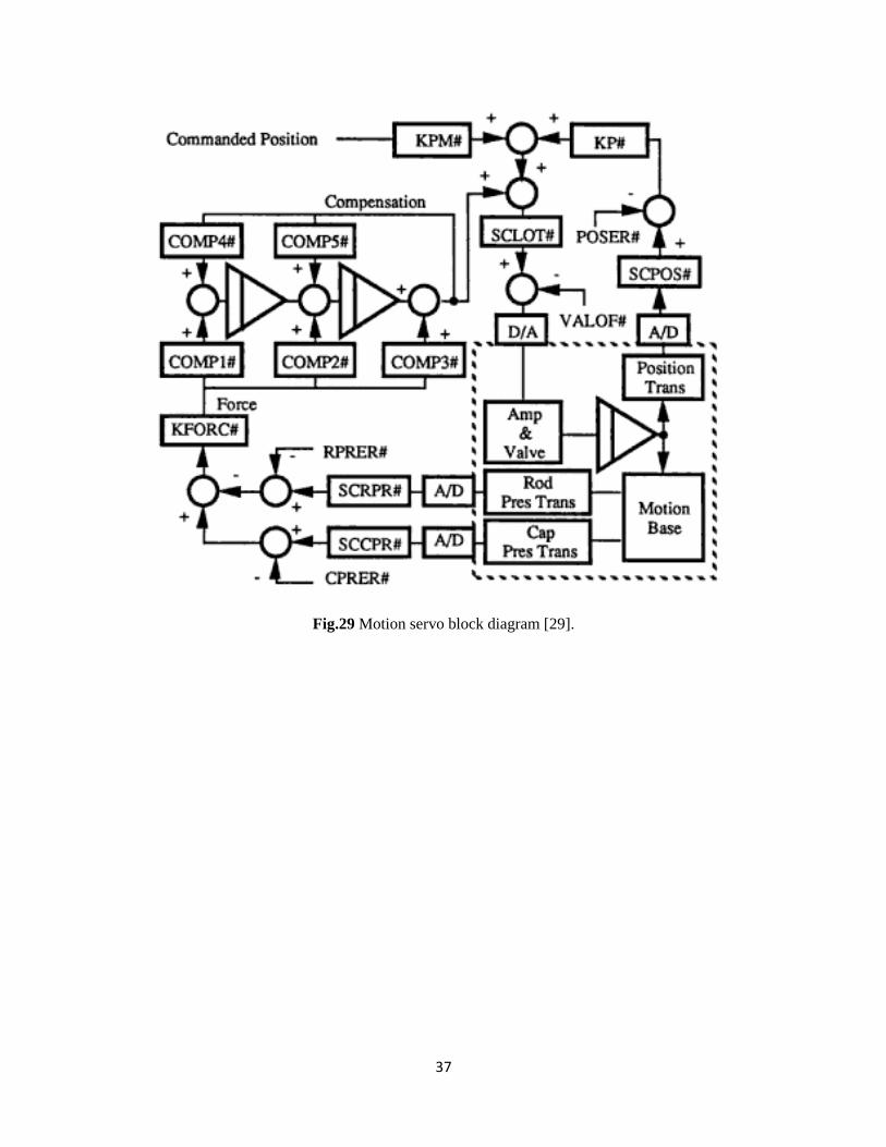
Reversible flight control systems: cockpit controls are directly mechanically linked with aircraft

control surfaces. Consequently, movement of the aerodynamic surface controls results in

movement of the cockpit controls Fig.30, and the aerodynamic forces feedback to the hands of

pilots directly.

Fig.30 Example of a typical reversible flight control system [26].

39

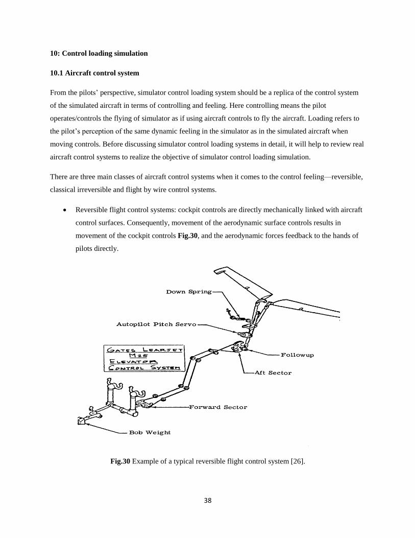
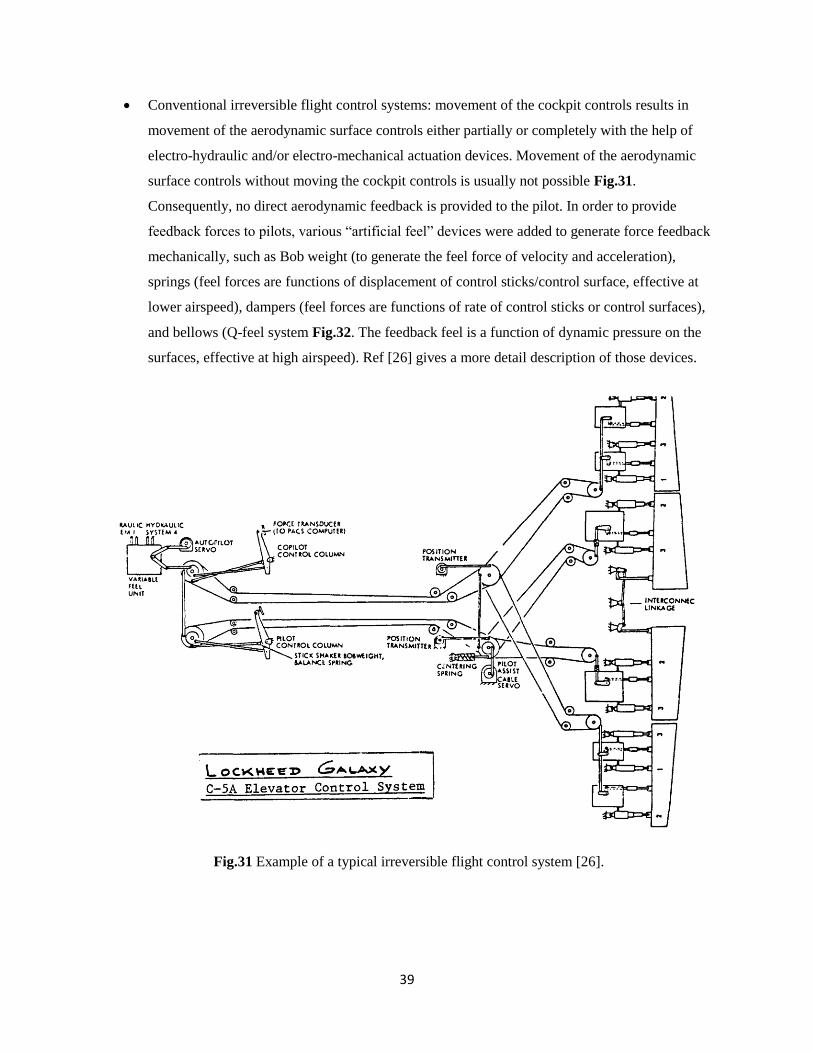
Conventional irreversible flight control systems: movement of the cockpit controls results in

movement of the aerodynamic surface controls either partially or completely with the help of

electro-hydraulic and/or electro-mechanical actuation devices. Movement of the aerodynamic

surface controls without moving the cockpit controls is usually not possible Fig.31.

Consequently, no direct aerodynamic feedback is provided to the pilot. In order to provide

feedback forces to pilots, various ―artificial feel‖ devices were added to generate force feedback

mechanically, such as Bob weight (to generate the feel force of velocity and acceleration),

springs (feel forces are functions of displacement of control sticks/control surface, effective at

lower airspeed), dampers (feel forces are functions of rate of control sticks or control surfaces),

and bellows (Q-feel system Fig.32. The feedback feel is a function of dynamic pressure on the

surfaces, effective at high airspeed). Ref [26] gives a more detail description of those devices.

Fig.31 Example of a typical irreversible flight control system [26].

40

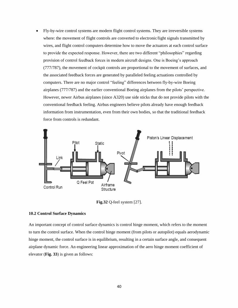
Fly-by-wire control systems are modern flight control systems. They are irreversible systems

where: the movement of flight controls are converted to electronic/light signals transmitted by

wires, and flight control computers determine how to move the actuators at each control surface

to provide the expected response. However, there are two different ―philosophies‖ regarding

provision of control feedback forces in modern aircraft designs. One is Boeing‘s approach

(777/787), the movement of cockpit controls are proportional to the movement of surfaces, and

the associated feedback forces are generated by paralleled feeling actuations controlled by

computers. There are no major control ―feeling‖ differences between fly-by-wire Boeing

airplanes (777/787) and the earlier conventional Boeing airplanes from the pilots‘ perspective.

However, newer Airbus airplanes (since A320) use side sticks that do not provide pilots with the

conventional feedback feeling. Airbus engineers believe pilots already have enough feedback

information from instrumentation, even from their own bodies, so that the traditional feedback

force from controls is redundant.

Fig.32 Q-feel system [27].

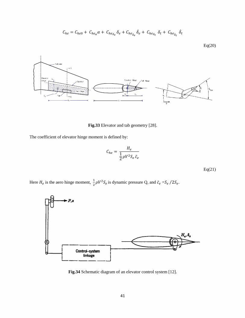
10.2 Control Surface Dynamics

An important concept of control surface dynamics is control hinge moment, which refers to the moment

to turn the control surface. When the control hinge moment (from pilots or autopilot) equals aerodynamic

hinge moment, the control surface is in equilibrium, resulting in a certain surface angle, and consequent

airplane dynamic force. An engineering linear approximation of the aero hinge moment coefficient of

elevator (Fig. 33) is given as follows:

41

Eq(20)

Fig.33 Elevator and tab geometry [28].

The coefficient of elevator hinge moment is defined by:

Eq(21)

Here is the aero hinge moment,

is dynamic pressure Q, and = .

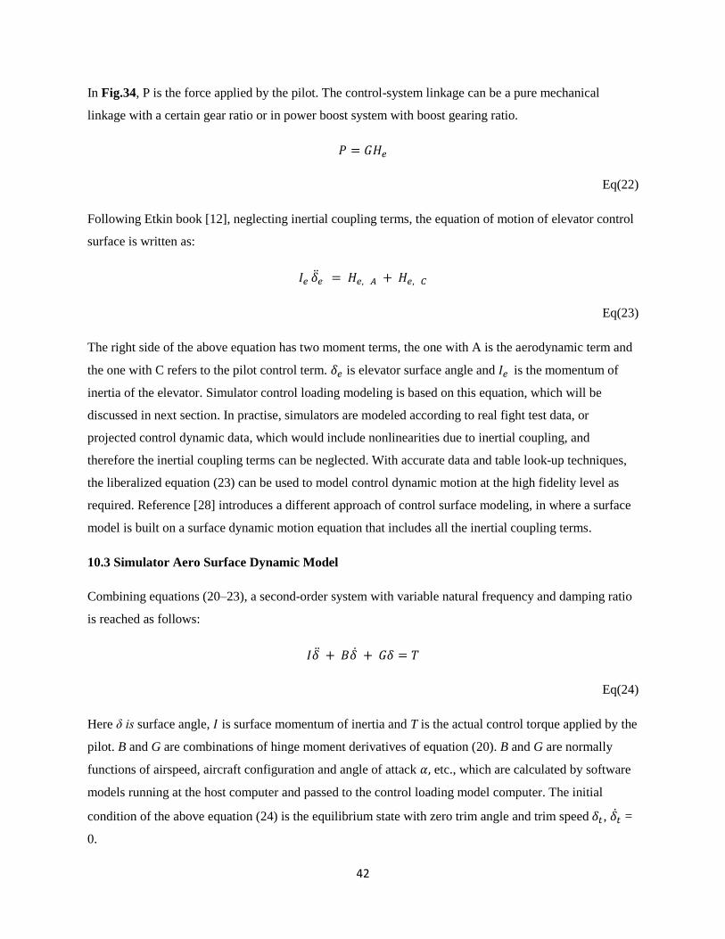
Fig.34 Schematic diagram of an elevator control system [12].

42

In Fig.34, P is the force applied by the pilot. The control-system linkage can be a pure mechanical

linkage with a certain gear ratio or in power boost system with boost gearing ratio.

Eq(22)

Following Etkin book [12], neglecting inertial coupling terms, the equation of motion of elevator control

surface is written as:

Eq(23)

The right side of the above equation has two moment terms, the one with A is the aerodynamic term and

the one with C refers to the pilot control term. is elevator surface angle and is the momentum of

inertia of the elevator. Simulator control loading modeling is based on this equation, which will be

discussed in next section. In practise, simulators are modeled according to real fight test data, or

projected control dynamic data, which would include nonlinearities due to inertial coupling, and

therefore the inertial coupling terms can be neglected. With accurate data and table look-up techniques,

the liberalized equation (23) can be used to model control dynamic motion at the high fidelity level as

required. Reference [28] introduces a different approach of control surface modeling, in where a surface

model is built on a surface dynamic motion equation that includes all the inertial coupling terms.

10.3 Simulator Aero Surface Dynamic Model

Combining equations (20–23), a second-order system with variable natural frequency and damping ratio

is reached as follows:

Eq(24)

Here δ is surface angle, is surface momentum of inertia and T is the actual control torque applied by the

pilot. B and G are combinations of hinge moment derivatives of equation (20). B and G are normally

functions of airspeed, aircraft configuration and angle of attack etc., which are calculated by software

models running at the host computer and passed to the control loading model computer. The initial

condition of the above equation (24) is the equilibrium state with zero trim angle and trim speed , =

0.

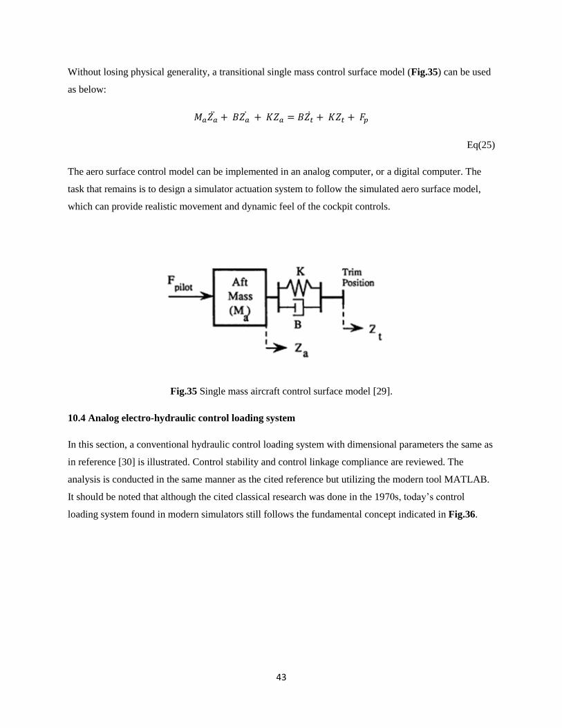
43

Without losing physical generality, a transitional single mass control surface model (Fig.35) can be used

as below:

Eq(25)

The aero surface control model can be implemented in an analog computer, or a digital computer. The

task that remains is to design a simulator actuation system to follow the simulated aero surface model,

which can provide realistic movement and dynamic feel of the cockpit controls.

Fig.35 Single mass aircraft control surface model [29].

10.4 Analog electro-hydraulic control loading system

In this section, a conventional hydraulic control loading system with dimensional parameters the same as

in reference [30] is illustrated. Control stability and control linkage compliance are reviewed. The

analysis is conducted in the same manner as the cited reference but utilizing the modern tool MATLAB.

It should be noted that although the cited classical research was done in the 1970s, today‘s control

loading system found in modern simulators still follows the fundamental concept indicated in Fig.36.

44

Fig.36 Electro-hydraulic control loading system [30].

As Fig.36 indicates, this control loading system includes two closed-loops. The inner loop is an electro-

hydraulic position control servo as described in part A of this thesis. The analog computer runs the aero

surface model defined by Eq (24). The analog model can be programmed to provide a wide range of

dynamic characteristics of control loads that occur in real aircraft. When the outer loop is closed, the

actuator follows the analog computer model. Basically the control law is reference model following. The

complexity of this system is that the output— (and also ), and input— are exerted in the same

place—the column. The pilot input force is sensed by a load cell; the same load cell that also senses

output acceleration.

Like any mechanical structure, the inherited natural frequency will cause resonance phenomena when the

appropriate conditions are satisfied, which could cause undesired low frequency oscillation and loading

effects in the output. One of important tasks is to eliminate these oscillations. Traditionally, compliant

factors are taken into consideration in designing control loading systems such as shown in Fig.37. The

hypothesis of mechanical compliance in the control linkage was substantiated by comparing the

behaviour of a mathematical model of the system with experimental data. The compliant linkage spring

rate and damping coefficient c are chosen to fit the experimental result. Both the model of rigid and

compliant linkage will be compared in the following section.

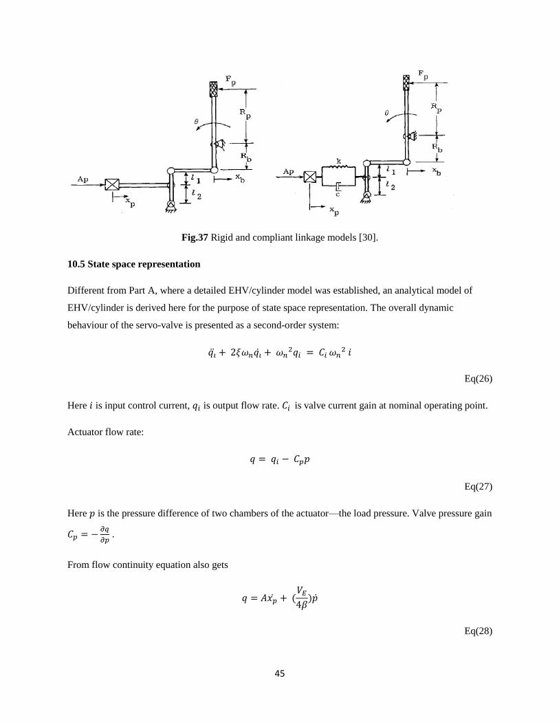
45

Fig.37 Rigid and compliant linkage models [30].

10.5 State space representation

Different from Part A, where a detailed EHV/cylinder model was established, an analytical model of

EHV/cylinder is derived here for the purpose of state space representation. The overall dynamic

behaviour of the servo-valve is presented as a second-order system:

Eq(26)

Here is input control current, is output flow rate. is valve current gain at nominal operating point.

Actuator flow rate:

Eq(27)

Here is the pressure difference of two chambers of the actuator—the load pressure. Valve pressure gain

.

From flow continuity equation also gets

Eq(28)

46

Here A is the actuator piston area, is the displacement of actuator piston, is the effective volume of

compressed fluid, and is the bulk modulus.

The control column dynamic

Eq(29)

Expressed in terms of the displacement of the base of the column

Eq(30)

Here is the lever arm of pilot force, is the lever arm of pilot force, is the linkage ratio, and is

the moment of inertia of column.

For rigid linkage model, the above equation can be expressed in terms of actuator displacement

Eq(31)

For complaint linkage, spring rate k and damping coefficient c have to be included in the equation

Eq(32)

Rearranged in the following manner

Eq(33)

Take a close look at the output of the linkage load cell, which inputs to the computer model. The model

equation is rewritten here

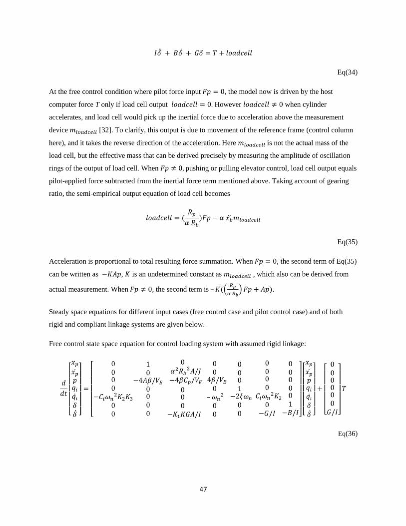
47

Eq(34)

At the free control condition where pilot force input , the model now is driven by the host

computer force T only if load cell output However when cylinder

accelerates, and load cell would pick up the inertial force due to acceleration above the measurement

device [32]. To clarify, this output is due to movement of the reference frame (control column

here), and it takes the reverse direction of the acceleration. Here is not the actual mass of the

load cell, but the effective mass that can be derived precisely by measuring the amplitude of oscillation

rings of the output of load cell. When pushing or pulling elevator control, load cell output equals

pilot-applied force subtracted from the inertial force term mentioned above. Taking account of gearing

ratio, the semi-empirical output equation of load cell becomes

Eq(35)

Acceleration is proportional to total resulting force summation. When , the second term of Eq(35)

can be written as , is an undetermined constant as , which also can be derived from

actual measurement. When , the second term is –

.

Steady space equations for different input cases (free control case and pilot control case) and of both

rigid and compliant linkage systems are given below.

Free control state space equation for control loading system with assumed rigid linkage:

–

Eq(36)

48

Free control state space equation for control loading system with assumed complaint linkage:

Eq(37)

Pilot control state space equation for control loading system with assumed rigid linkage:

–

Eq(38)

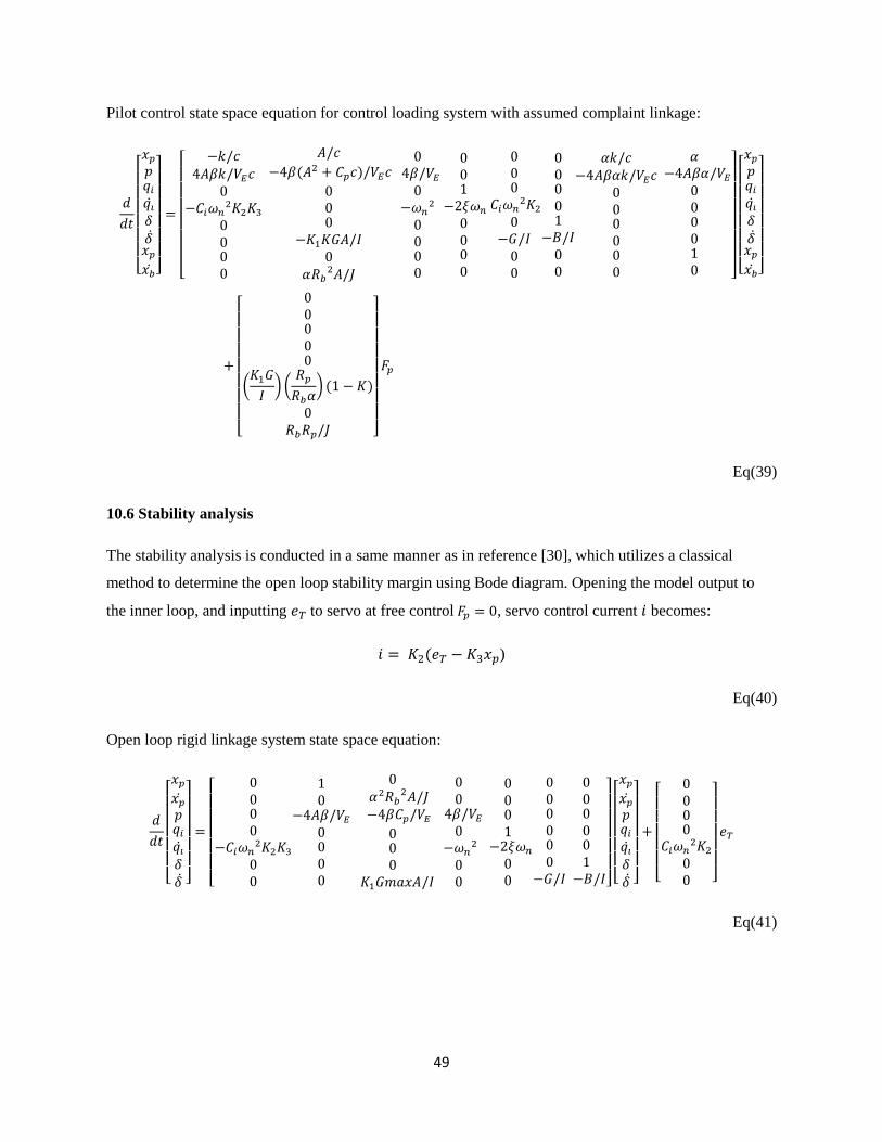
49

Pilot control state space equation for control loading system with assumed complaint linkage:

Eq(39)

10.6 Stability analysis

The stability analysis is conducted in a same manner as in reference [30], which utilizes a classical

method to determine the open loop stability margin using Bode diagram. Opening the model output to

the inner loop, and inputting to servo at free control , servo control current becomes:

)

Eq(40)

Open loop rigid linkage system state space equation:

Eq(41)

50

Open loop compliant linkage system state space equation:

Eq(42)

The resulting Bode diagram (Fig.45) depicts both rigid and compliant systems‘ frequency responses

for easy comparison. The particular simulated mode with parameters ,

, . It clearly indicates that the compliance of linkage results in

insatiability at a frequency of about 12 Hz. In simulators, periodically pushing/pulling at certain

frequencies could excite control oscillation, and eventually triggers a safety protection circuit that is

designed to power off the control loading when the oscillation exceeds its limits. A qualitative

explanation is that the natural frequency of the mechanical system is excited, causing resonance.

Fig.38 Bode diagram (open outer loop).

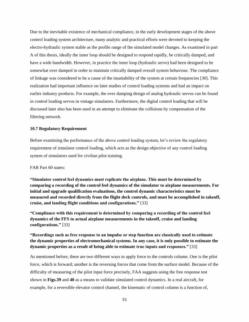
51

Due to the inevitable existence of mechanical compliance, in the early development stages of the above

control loading system architecture, many analytic and practical efforts were devoted to keeping the

electro-hydraulic system stable as the profile range of the simulated model changes. As examined in part

A of this thesis, ideally the inner loop should be designed to respond rapidly, be critically damped, and

have a wide bandwidth. However, in practice the inner loop (hydraulic servo) had been designed to be

somewhat over damped in order to maintain critically damped overall system behaviour. The compliance

of linkage was considered to be a cause of the insatiability of the system at certain frequencies [30]. This

realization had important influence on later studies of control loading systems and had an impact on

earlier industry products. For example, the over damping design of analog hydraulic servos can be found

in control loading servos in vintage simulators. Furthermore, the digital control loading that will be

discussed later also has been used in an attempt to eliminate the collisions by compensation of the

filtering network.

10.7 Regulatory Requirement

Before examining the performance of the above control loading system, let‘s review the regulatory

requirement of simulator control loading, which acts as the design objective of any control loading

system of simulators used for civilian pilot training.

FAR Part 60 states:

“Simulator control feel dynamics must replicate the airplane. This must be determined by

comparing a recording of the control feel dynamics of the simulator to airplane measurements. For

initial and upgrade qualification evaluations, the control dynamic characteristics must be

measured and recorded directly from the flight deck controls, and must be accomplished in takeoff,

cruise, and landing flight conditions and configurations.” [33]

“Compliance with this requirement is determined by comparing a recording of the control feel

dynamics of the FFS to actual airplane measurements in the takeoff, cruise and landing

configurations.” [33]

“Recordings such as free response to an impulse or step function are classically used to estimate

the dynamic properties of electromechanical systems. In any case, it is only possible to estimate the

dynamic properties as a result of being able to estimate true inputs and responses.” [33]

As mentioned before, there are two different ways to apply force to the controls column. One is the pilot

force, which is forward; another is the reversing forces that come from the surface model. Because of the

difficulty of measuring of the pilot input force precisely, FAA suggests using the free response test

shown in Figs.39 and 40 as a means to validate simulated control dynamics. In a real aircraft, for

example, for a reversible elevator control channel, the kinematic of control column is a function of,

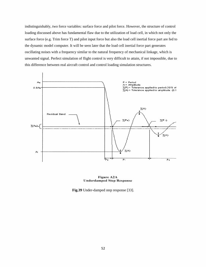
52

indistinguishably, two force variables: surface force and pilot force. However, the structure of control

loading discussed above has fundamental flaw due to the utilization of load cell, in which not only the

surface force (e.g. Trim force T) and pilot input force but also the load cell inertial force part are fed to

the dynamic model computer. It will be seen later that the load cell inertial force part generates

oscillating noises with a frequency similar to the natural frequency of mechanical linkage, which is

unwanted signal. Perfect simulation of flight control is very difficult to attain, if not impossible, due to

this difference between real aircraft control and control loading simulation structures.

Fig.39 Under-damped step response [33].

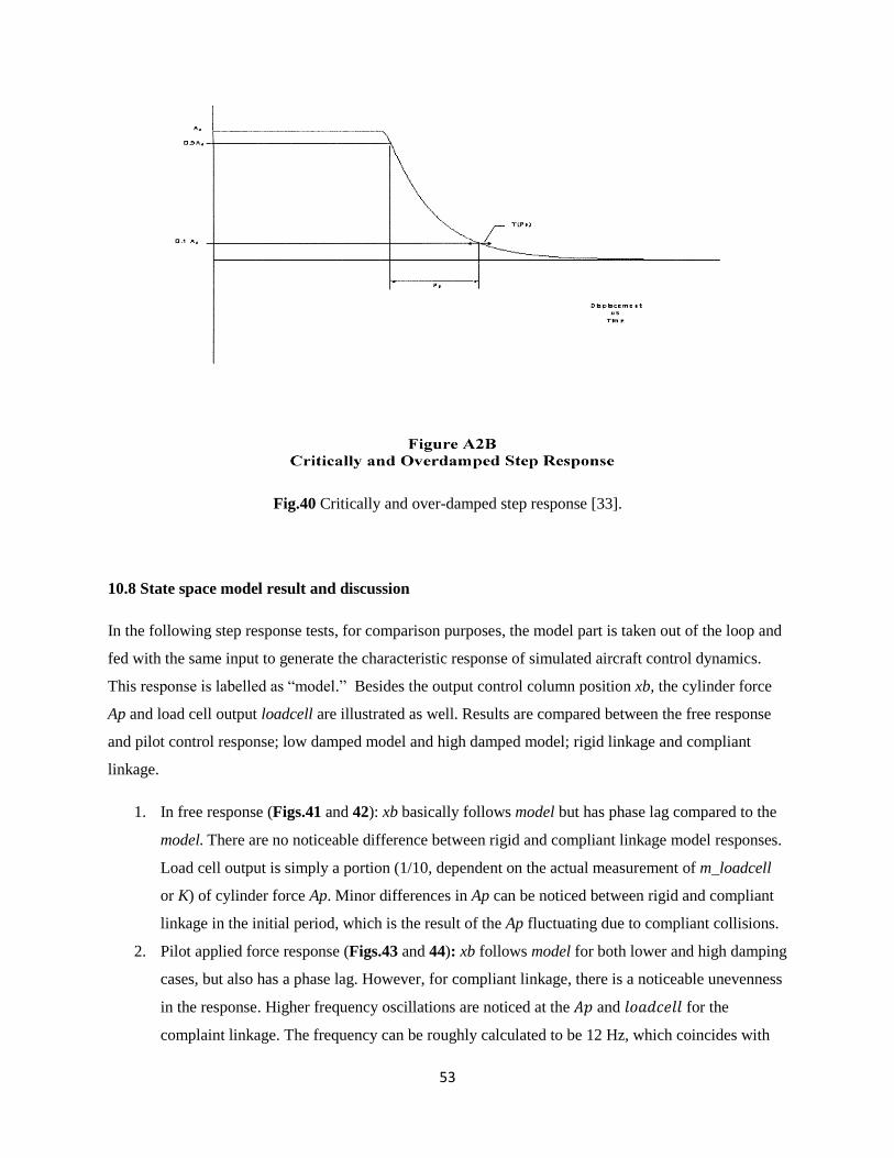
53

Fig.40 Critically and over-damped step response [33].

10.8 State space model result and discussion

In the following step response tests, for comparison purposes, the model part is taken out of the loop and

fed with the same input to generate the characteristic response of simulated aircraft control dynamics.

This response is labelled as ―model.‖ Besides the output control column position xb, the cylinder force

Ap and load cell output loadcell are illustrated as well. Results are compared between the free response

and pilot control response; low damped model and high damped model; rigid linkage and compliant

linkage.

1. In free response (Figs.41 and 42): xb basically follows model but has phase lag compared to the

model There are no noticeable difference between rigid and compliant linkage model responses.

Load cell output is simply a portion (1/10, dependent on the actual measurement of m_loadcell

or K) of cylinder force Ap. Minor differences in Ap can be noticed between rigid and compliant

linkage in the initial period, which is the result of the Ap fluctuating due to compliant collisions.

2. Pilot applied force response (Figs.43 and 44): xb follows model for both lower and high damping

cases, but also has a phase lag. However, for compliant linkage, there is a noticeable unevenness

in the response. Higher frequency oscillations are noticed at the and for the

complaint linkage. The frequency can be roughly calculated to be 12 Hz, which coincides with

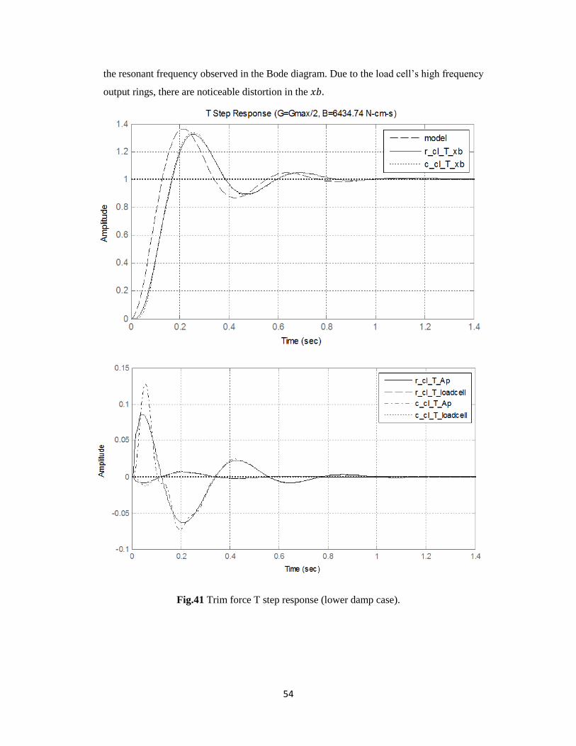
54

the resonant frequency observed in the Bode diagram. Due to the load cell‘s high frequency

output rings, there are noticeable distortion in the

Fig.41 Trim force T step response (lower damp case).

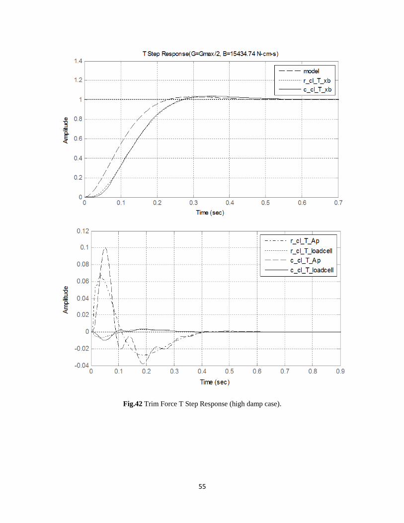
55

Fig.42 Trim Force T Step Response (high damp case).

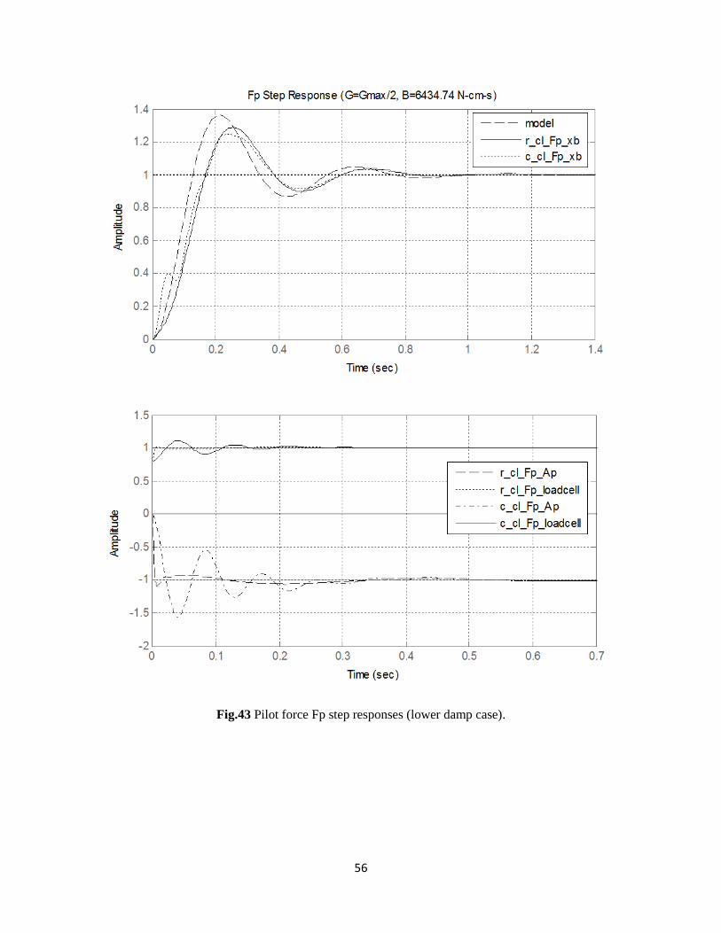
56

Fig.43 Pilot force Fp step responses (lower damp case).

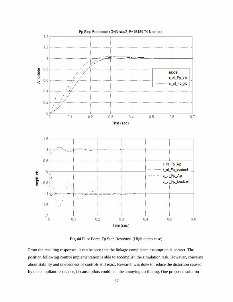
57

Fig.44 Pilot Force Fp Step Response (High damp case).

From the resulting responses, it can be seen that the linkage compliance assumption is correct. The

position following control implementation is able to accomplish the simulation task. However, concerns

about stability and unevenness of controls still exist. Research was done to reduce the distortion caused

by the compliant resonance, because pilots could feel the annoying oscillating. One proposed solution

58

was to use state feedback networked with a gain matrix optimized by quadratic optimal method [30]. The

optimization computing was resorted to as a discrete dynamic programming algorithm, which can reach

a result similar to that of using the MATLAB command lpr, but is much more tedious. This proposed

new structure has influenced the next generation of digital control loading systems.

10.9 Control loading Simulink Model

Simulink modeling of control loading utilizes the resultant EHV/cylinder model that was developed in

Part A. The EHV/cylinder Simulink model that was developed is plugged into the same control loading

channel discussed in previous sections. The compliance of linkage is also taken into account. A

symbolical model with the same control implementation—model position following—is constructed first,

then followed by a different control scheme implementation—model velocity following.

The linkage model is demonstrated in Fig.45. It includes the model of compliance of linkage with a

natural frequency of 12 Hz. It has also incorporated the semi-empirical load cell model. The assumption

is that the linkage is frictionless in both static and Coulomb. It must be noted that frictions that exist in

real aircraft control channels could be simulated by particular software algorithms and sent to the control

loading by the host computer, which is different from that of the control loading linkage. Certainly the

load cell will affected by the friction force. However, in normal working conditions, the friction

concerned is very small, and can be safety ignored. When the friction of the linkage becomes abnormal,

in some cases, pilot can ―feel‖ it, which indicates that control loading system maintenance is required.

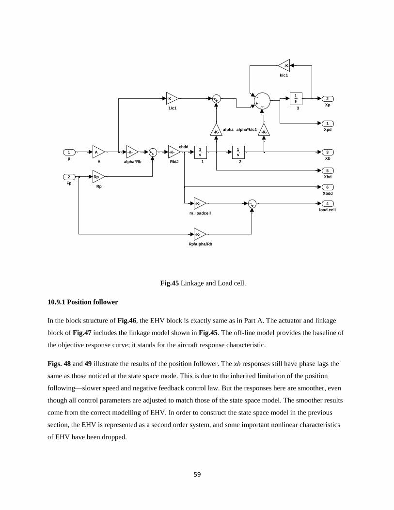
59

Fig.45 Linkage and Load cell.

10.9.1 Position follower

In the block structure of Fig.46, the EHV block is exactly same as in Part A. The actuator and linkage

block of Fig.47 includes the linkage model shown in Fig.45. The off-line model provides the baseline of

the objective response curve; it stands for the aircraft response characteristic.

Figs. 48 and 49 illustrate the results of the position follower. The xb responses still have phase lags the

same as those noticed at the state space mode. This is due to the inherited limitation of the position

following—slower speed and negative feedback control law. But the responses here are smoother, even

though all control parameters are adjusted to match those of the state space model. The smoother results

come from the correct modelling of EHV. In order to construct the state space model in the previous

section, the EHV is represented as a second order system, and some important nonlinear characteristics

of EHV have been dropped.

xbdd

6

Xbdd

5

Xbd

4

load cell

3

Xb

2

Xp

1

Xpd

-K-

m_loadcell

-K-

k/c1

-K-alpha*k/c1

-K-

alpha*Rb

-K-alpha

-K-

Rp/alpha/Rb

Rp

Rp

-K-

Rb/J

A

A

-K-

1/c1

1

s

3

1

s

2

1

s

1

2

Fp

1

p

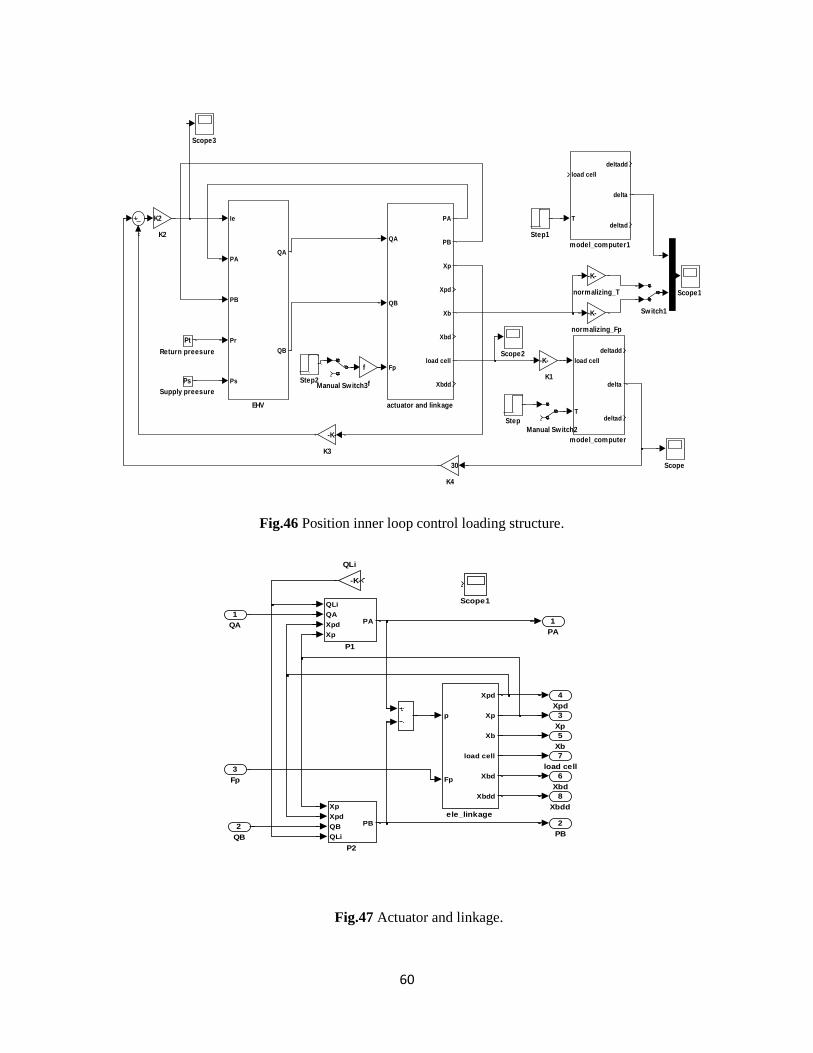
60

Fig.46 Position inner loop control loading structure.

Fig.47 Actuator and linkage.

-K-

normalizing_T

-K-

normalizing_Fp

load cell

T

deltadd

delta

deltad

model_computer1

load cell

T

deltadd

delta

deltad

model_computer

f

f

QA

QB

Fp

PA

PB

Xp

Xpd

Xb

Xbd

load cell

Xbdd

actuator and linkage

Switch1

Ps

Supply preesure

Step2

Step1

Step

Scope3

Scope2

Scope1

Scope

Pt

Return preesure

Manual Switch3

Manual Switch2

30

K4

-K-

K3

K2

K2

-K-

K1

Ie

PA

PB

Pr

Ps

QA

QB

EHV

8

Xbdd

7

load cell

6

Xbd

5

Xb

4

Xpd

3

Xp

2

PB

1

PA

p

Fp

Xpd

Xp

Xb

load cell

Xbd

Xbdd

ele_linkage

Scope1

-K-

QLi

Xp

Xpd

QB

QLi

PB

P2

QLi

QA

Xpd

Xp

PA

P1

3

Fp

2

QB

1

QA

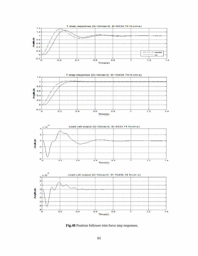
61

Fig.48 Position follower trim force step responses.

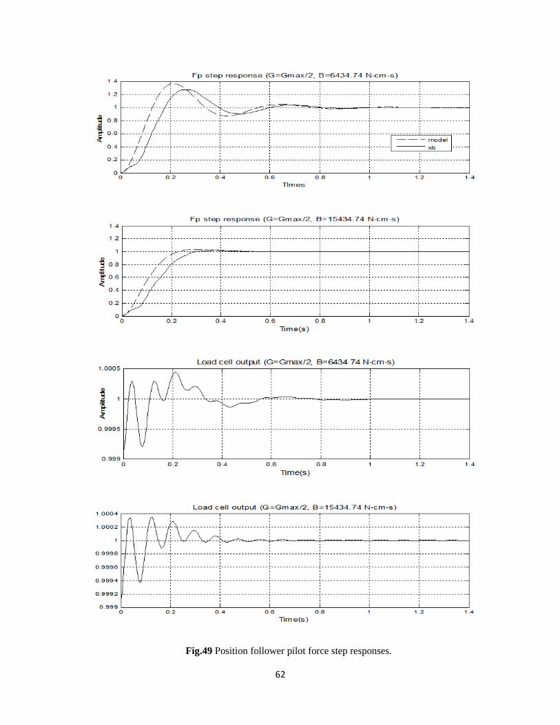
62

Fig.49 Position follower pilot force step responses.

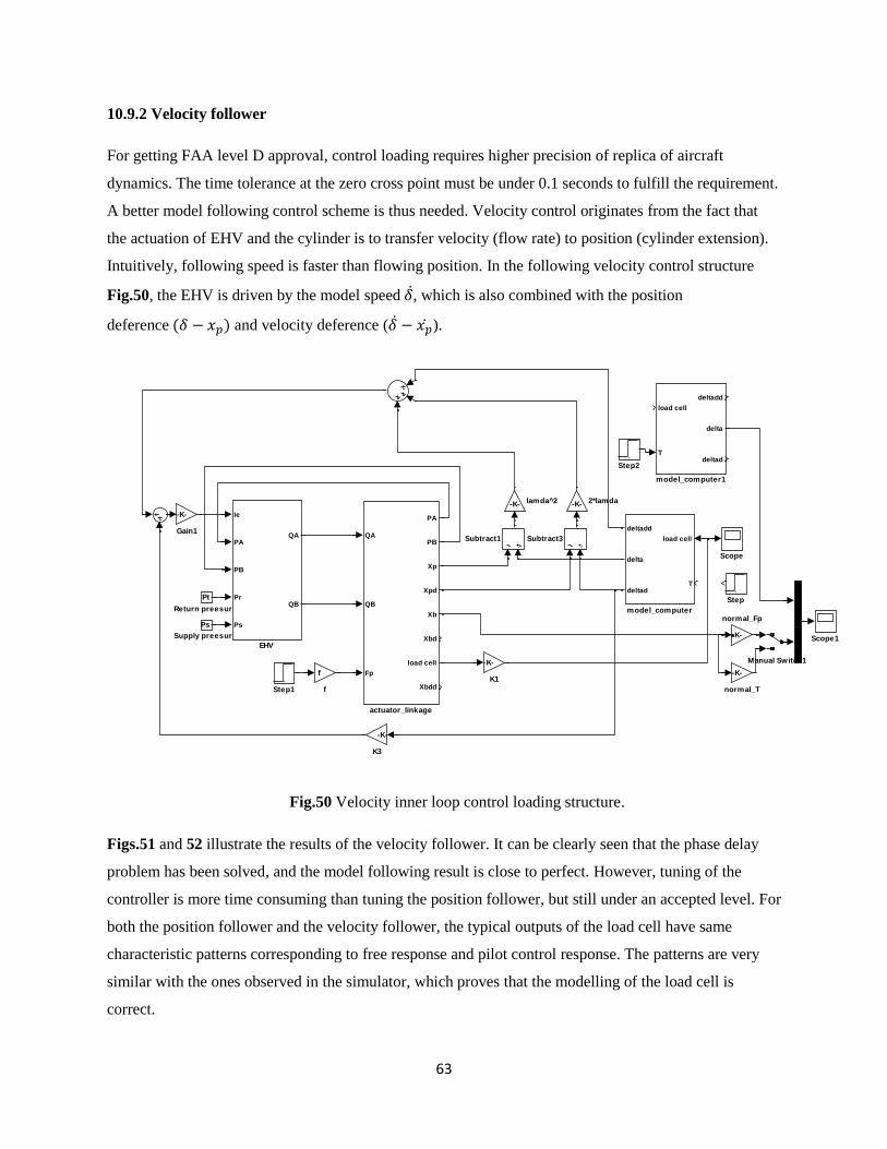
63

10.9.2 Velocity follower

For getting FAA level D approval, control loading requires higher precision of replica of aircraft

dynamics. The time tolerance at the zero cross point must be under 0.1 seconds to fulfill the requirement.

A better model following control scheme is thus needed. Velocity control originates from the fact that

the actuation of EHV and the cylinder is to transfer velocity (flow rate) to position (cylinder extension).

Intuitively, following speed is faster than flowing position. In the following velocity control structure

Fig.50, the EHV is driven by the model speed , which is also combined with the position

deference and velocity deference ( ).

Fig.50 Velocity inner loop control loading structure.

Figs.51 and 52 illustrate the results of the velocity follower. It can be clearly seen that the phase delay

problem has been solved, and the model following result is close to perfect. However, tuning of the

controller is more time consuming than tuning the position follower, but still under an accepted level. For

both the position follower and the velocity follower, the typical outputs of the load cell have same

characteristic patterns corresponding to free response and pilot control response. The patterns are very

similar with the ones observed in the simulator, which proves that the modelling of the load cell is

correct.

-K-

normal_T

-K-

normal_Fp

load cell

T

deltadd

delta

deltad

model_computer1

load cell

T

deltadd

delta

deltad

model_computer

-K- lamda^2

f

f

QA

QB

Fp

PA

PB

Xp

Xpd

Xb

Xbd

load cell

Xbdd

actuator_linkage

Ps

Supply preesure

Subtract3Subtract1

Step2

Step1

Step

Scope1

Scope

Pt

Return preesure

Manual Switch1

-K-

K3

-K-

K1

-K-

Gain1

Ie

PA

PB

Pr

Ps

QA

QB

EHV

-K- 2*lamda

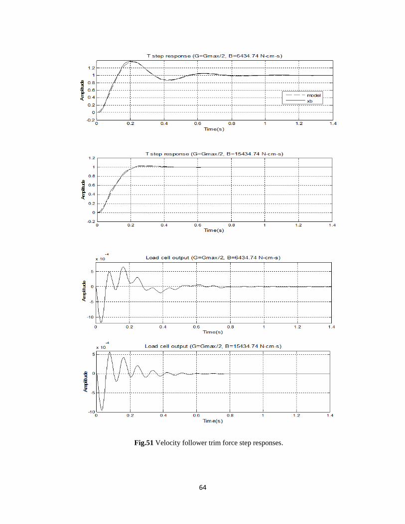
64

Fig.51 Velocity follower trim force step responses.

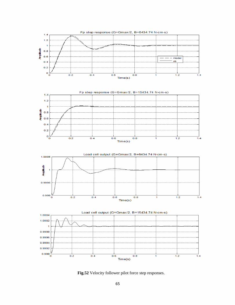
65

Fig.52 Velocity follower pilot force step responses.

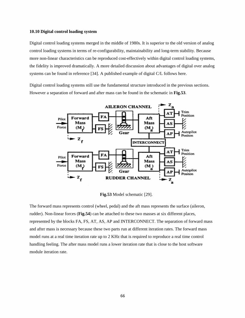
66

10.10 Digital control loading system

Digital control loading systems merged in the middle of 1980s. It is superior to the old version of analog

control loading systems in terms of re-configurability, maintainability and long-term stability. Because

more non-linear characteristics can be reproduced cost-effectively within digital control loading systems,

the fidelity is improved dramatically. A more detailed discussion about advantages of digital over analog

systems can be found in reference [34]. A published example of digital C/L follows here.

Digital control loading systems still use the fundamental structure introduced in the previous sections.

However a separation of forward and after mass can be found in the schematic in Fig.53.

Fig.53 Model schematic [29].

The forward mass represents control (wheel, pedal) and the aft mass represents the surface (aileron,

rudder). Non-linear forces (Fig.54) can be attached to these two masses at six different places,

represented by the blocks FA, FS, AT, AS, AP and INTERCONNECT. The separation of forward mass

and after mass is necessary because these two parts run at different iteration rates. The forward mass

model runs at a real time iteration rate up to 2 KHz that is required to reproduce a real time control

handling feeling. The after mass model runs a lower iteration rate that is close to the host software

module iteration rate.

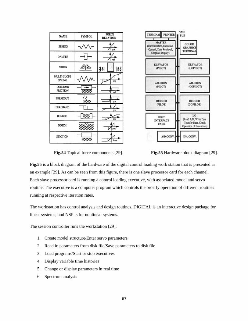
67

Fig.54 Topical force components [29]. Fig.55 Hardware block diagram [29].

Fig.55 is a block diagram of the hardware of the digital control loading work station that is presented as

an example [29]. As can be seen from this figure, there is one slave processor card for each channel.

Each slave processor card is running a control loading executive, with associated model and servo

routine. The executive is a computer program which controls the orderly operation of different routines

running at respective iteration rates.

The workstation has control analysis and design routines. DIGITAL is an interactive design package for

linear systems; and NSP is for nonlinear systems.

The session controller runs the workstation [29]:

1. Create model structure/Enter servo parameters

2. Read in parameters from disk file/Save parameters to disk file

3. Load programs/Start or stop executives

4. Display variable time histories

5. Change or display parameters in real time

6. Spectrum analysis

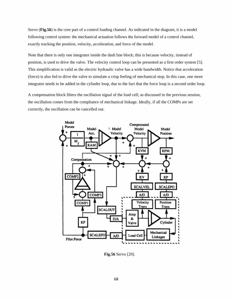
68

Servo (Fig.56) is the core part of a control loading channel. As indicated in the diagram, it is a model

following control system: the mechanical actuation follows the forward model of a control channel,

exactly tracking the position, velocity, acceleration, and force of the model.

Note that there is only one integrator inside the dash line block; this is because velocity, instead of

position, is used to drive the valve. The velocity control loop can be presented as a first order system [5].

This simplification is valid as the electric hydraulic valve has a wide bandwidth. Notice that acceleration

(force) is also fed to drive the valve to simulate a crisp feeling of mechanical stop. In this case, one more

integrator needs to be added in the cylinder loop, due to the fact that the force loop is a second order loop.

A compensation block filters the oscillation signal of the load cell; as discussed in the previous session,

the oscillation comes from the compliance of mechanical linkage. Ideally, if all the COMPs are set

correctly, the oscillation can be cancelled out.

Fig.56 Servo [29].

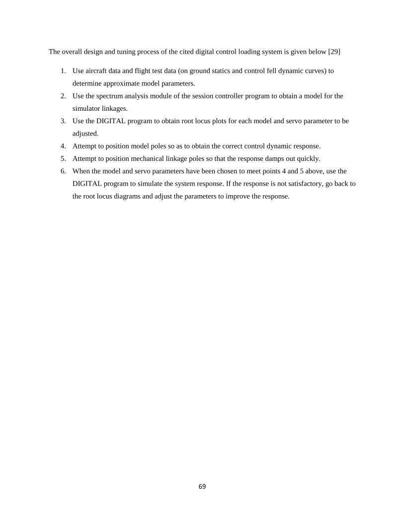
69

The overall design and tuning process of the cited digital control loading system is given below [29]

1. Use aircraft data and flight test data (on ground statics and control fell dynamic curves) to

determine approximate model parameters.

2. Use the spectrum analysis module of the session controller program to obtain a model for the

simulator linkages.

3. Use the DIGITAL program to obtain root locus plots for each model and servo parameter to be

adjusted.

4. Attempt to position model poles so as to obtain the correct control dynamic response.

5. Attempt to position mechanical linkage poles so that the response damps out quickly.

6. When the model and servo parameters have been chosen to meet points 4 and 5 above, use the

DIGITAL program to simulate the system response. If the response is not satisfactory, go back to

the root locus diagrams and adjust the parameters to improve the response.

70

11: Electrical control loading and motion

There is always room for improvement. In 2006, the world‘s first electrical motion and control loading

full-flight simulator was honoured with a Level D certificate by FAA. While it fully met the performance

specifications, the advantages that electrical motion and control loading bring to the pilot training

industry are [35]

Higher energy efficiency of up to 80% over the hydraulic counterpart. This is because electrical

systems do not need to maintain a high hydraulic pressure source.

Higher uptime from maintenance. Maintenance of hydraulic system is tedious and both labour

and materials are costly compared to that of electric systems.

Less-costly infrastructure, because there is no need to build a hydraulic pressure supply room

and hydraulic hoses ditches.

More environmentally friendly, due to the lack of hydraulic fluid leak, and the lack of noise

generated from hydraulic pressure pump.

Just like any technical innovation, the development of electrical motion and control loading faced

challenges. For motion systems, the plant ( simulator platform) has a very high payload, which was never

a problem for hydraulic cylinders due to their big power factor; and there is a safety issue when

electricity power is interrupted, which wasn‘t a problem for hydraulic system because the pressure

reserved in hydraulic accumulators could bring the simulator back to its ‗parking‘ position. For control

loading, there were concerns about the residual torques of the motor, which might be felt around the

control center position.

Inspired by industry demand initiative, engineers have resolved those challenges. With the help of

advances in processing technology and high-power devices techniques, high-power servo-drives have

been developed; high-energy magnets have boosted power density in brushless motors; ball-screw

technology devices have been used to translate rotation into linear movement; and a special cushion has

been designed to prevent the actuators from damaging the end stop [35]. All the efforts make up the most

important component—electric actuators. For control loading, model-follower force-loop technology has

been implemented. Linear electric actuators that are used for primary control are equipped with position

feedback encoders [36].

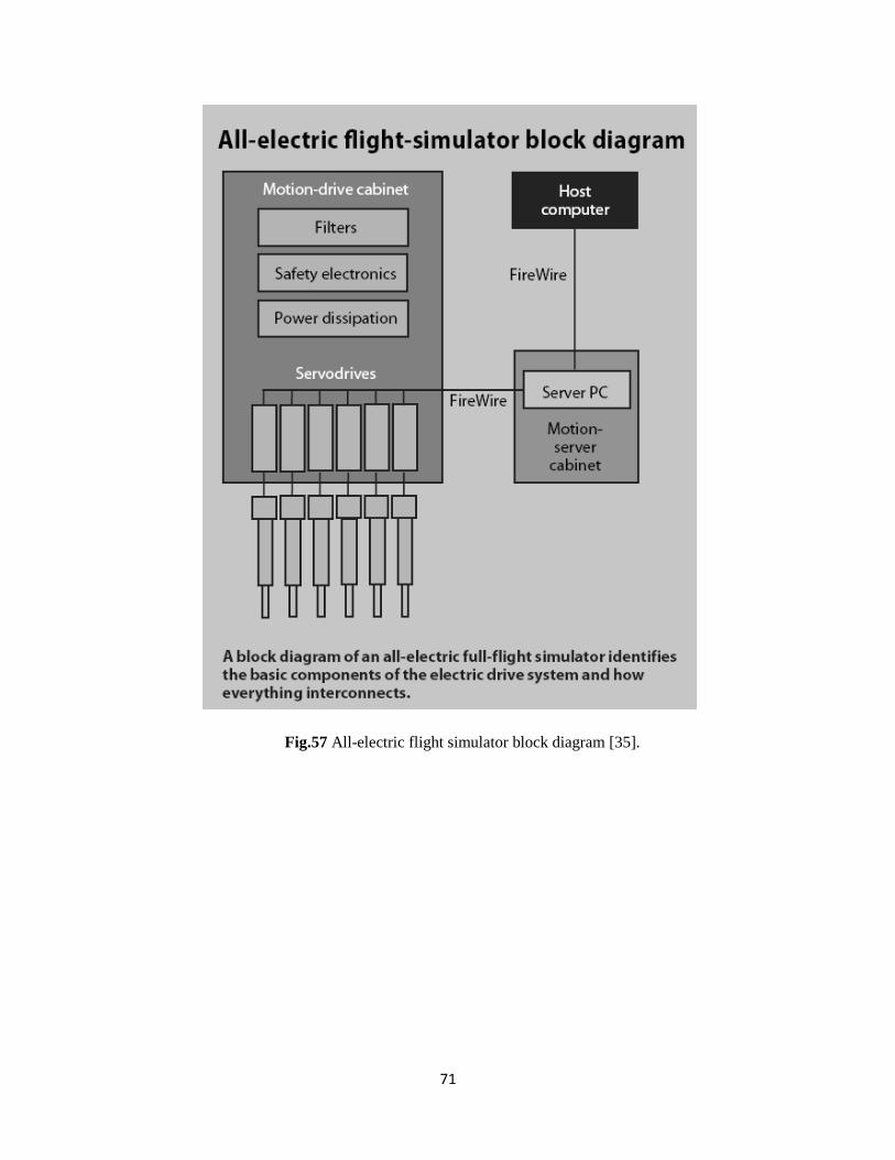
71

Fig.57 All-electric flight simulator block diagram [35].

72

12: Conclusion

A generic approach is proposed to study the aircraft motion and control loading simulation with a

particular focus on simulation algorithms and control scheme implementations. This approach has

greatly improved the understanding of this subject.

As the core part of this project, the symbolic modelling of control loading channels by Simulink is

effective and validated. In industry practice, control loading model tuning and control parameter tuning

are tedious and time-consuming tasks. One reason for this is the uncertainty of output of the load cell.

Ideally, the output of the load cell is the pilot input force. But in reality, as can be observed in flight

simulators, there are unwanted rings or oscillating ―noise‖ existing with pilot force output. The load cell

outputs modelling simulation results (Figs.51 and 52) are similar to the ones observed in simulators. The

analytical correctness comes from the detailed model of EHV/actuator, the consideration of linkage

compliance, and the correct mathematical modelling of the load cell. To the author‘s knowledge, this

particular mathematical modelling had never been presented in any of the referenced works of this thesis.

The significance of the model is that a filtering method can be developed based on the analytical result of

load cell; eventually a perfect matching between model and actuation can be achieved cost-effectively by

filtering unwanted signals.

Reviewing the history of aircraft motion and control simulation: from simplest man-power to hydraulic

power and on to electrical power; from analog model/servo to digital model/servo; from position-loop to

velocity loop and to force-loop, the fulfilling of industry demands with available resources takes priority

than the pursuing of technical performance. The construction and control parameter tuning of the

different model followers during this research revealed the design of control simulation is an iterative

and optimizing process, and is a trade-off between the control performance, cost, maintainability, and the

ease of tuning. The researches of this thesis provide an effective means and platform for further design

optimization, system reliability, and prognostic analyses.

The accuracy of the motion simulation algorithm is dependent on the accuracy of the theory of motion

cue perception mechanisms of human beings. It can be speculated that the next generation of motion

simulation will benefit from the latest psychophysical research results of human sensory mechanisms

about visual, motion and tactile cues. For control dynamic simulation, the MRAC (model-reference

adaptive control) technique theoretically can reach perfect model following. However the bottle-neck is

to sense all the required feedback signals accurately, especially force or acceleration, using cost-efficient

methods. The motion and control loading models presented in this thesis also can be utilized for the

73

research of next generation motion simulation, for designing control observers, and for testing different

position transducers.

74

References

[1] H. Schlichting, Boundary-Layer Theory, 7th

Ed. Mcgraw-Hill, 1979, p. 1.

[2] R. C. A‘Harrah, Flight Simulation, Past, Present, and Future, AIAA Paper No. 65-480, AIAA

Second Annual Meeting, San Francisco, CA, 1965, pp. 371-386.

[3] J. M. Rolfe, K. J. Staples, Flight Simulation, Cambridge, London, 1986, pp.79, 86, 111-122.

[4]Moog Inc., Moog 760 Series Servovalves, Moog Inc., 2007, pp. 2-4.

[5] N. D. Manring, Hydraulic Control Systems, John Wiley & Sons, Inc., 2005, Chapter 7.

[6] M. G. Rabie, Fluid Power Engineering, Mcgraw-Hill, 2009, Chapter 10.

[7] M. Kalyoncu, M. Haydim, ―Mathematical Modelling and fuzzy logic based position control of an

electrohydraulic servosystem with internal leakage,‖ Mechatronics, 19, 2009, pp. 847-858.

[8] R. Poley, DSP Control of Electro-Hydraulic Servo Actuators, Texas Instruments Application Report,

2005.

[9] D. Allerton, Principles of Flight Simulation, John Wiley & Sons, Inc. 2009, p. 429.

[10] H. E. Merritt, Hydraulic Control Systems, Wiley, 1967, pp. 39-43.

[11] Moog Inc.. Electrohydraulic Valve, A Technical Look. Retrieved March 8, 2010, from

http://www.moog.com/literature/ICD/Valves-Introduction.pdf

[12] B. Etkin, Dynamics of Flight, Stability and Control, John Wiley & Sons, 1996, Chapter 4, 7.

[13] Wikipedia, Pictures, Retrieved March 8, 2010, from http://en.wikipedia.org/wiki/Flight_simulator

[14] Wikipedia, Acceleration onset cueing, Retrieved July 8, 2010, from

http://en.wikipedia.org/wiki/Acceleration_onset_cueing

75

[15] C. C. Clark, Human control performance and tolerance under severe complex wave form vibration

and review of flight simulation, with a preliminary historic review of flight simulation, Accession No.

62N14482, NASA 1962, pp. 176-194.

[16] L. D. Reid, M. A. Nahon, ―Response of airline pilots to variations in flight simulator motion

algorithms,‖Journal of Aircraft, 25 (7), 1988, pp. 639–646.

[17] R. J. A. W. Hosman, J. C. van der Vaart, Thresholds of Motion Perception and Parameters of

Vestibular Models Obtained from Test in a Motion simulator, Effects of Vestibular and Motion

Perception on Task Performance, Memorandum M-372. Delft, Technische Hogeschool Delft, 1980.

[18] J. L. Meiry, The Vestibular System and Human Dynamic Space Orientation, Report No. NASA-CR-

122692,T-65-1, NASA, 1966.

[19] C. C. Ormsby, Model of Human Dynamic Orientation, Report No. NASA-CR-132537, NASA, 1974.

[20] D. Stewart, ―A platform with six-degree-of-freedom,‖ Proceedings in the Institution of mechanical

Engineers, 180, 1(5), 1965, pp.371-386.

[21] M. A. Nahon, L. D. Reid, ―Adaptive Simulator Motion Software with Supervisory Control,‖

Journal of Guidance, Control, and Dynamics, 15(2), 1992, pp. 376-383.

[22] M. A. Nahon, L. D. Reid, “Simulator Motion-drive Algorithms: A designer‘s Perspective,” Journal

of Guidance, Control, and Dynamics, 13(2), 1990, pp. 356-362.

[23] S. K. Advani, M. A. Nahon, N. Haeck, J. Albronda, ―Optimization of Six-Degrees-of-Freedom

Motion Systems for Flight Simulators,‖ Journal of Aircraft, 36(5), 1997, pp. 819-826.

[24] M. Idan, D. Sahar, Robust controller for a dynamic six degree of freedom flight simulator, AIAA

Flight Simulation Technologies Conference, San Diego, CA, July 1996.

[25] P. R. Grant, S. K. Advani, An Iterative Learning Control Algorithm for Simulator Motion System

Control, AIAA Modeling and Simulation Technologies Conference and Exhibit, Hilton Head, SC,

August 2007.

76

[26] J. Roskam, Airplane Flight Dynamics and Automatic Flight Controls, Roskam Aviation and

Engineering Corporation, 1979, pp. 300-305.

[27] Jeppesen Sanderson, Inc., Airframes and Systems, Jeppesen, Sanderson, Inc., 2005, p. (5)33.

[28] D. P. Coiro, A. De Marco, F. Nicolosi, A 6DOF Flight Simulation Environment for General

Aviation Aircraft with Control Loading Reproduction, AIAA Modeling and Simulation Technologies

Conference and Exhibit, Hilton Head, SC, August 2007.

[29] M. T. Hagan, J. O. Hamalainen, N. M. Sammur, G. Guimaraes, C. D. Latino, ―Digital control

loading and motion for flight simulation,‖ Progress in simulation, Volume 2, edited by G. W. Zobrist, J.

V. Leonard, 1994, pp. 52-87.

[30] P. R. Johansen, R. E. Bardusc, Analysis and compensation of an aircraft simulator control loading

system with compliant linkage, NASA TN D-7747, 1974.

[31] R. V. P., Billy R. Asbworth, The effect odd digital computing on the performance of a closed-loop

control-loading system, NASA TN D-8371, 1976.

[32] A. Gerretsen, M. Mulder, M.M. van Paassen, Comparison of position-loop, velocity-loop and force-

loop based control loading architectures, AIAA Modeling and Simulation Technologies Conference and

Exhibit, San Francisco, CA, August 2005.

[33] National Simulator Program, 14 CFR Part 60 NSP Consolidated Version, Retrieved March8, 2010,

from http://www.faa.gov/about/initiatives/nsp/media/consolidated_version.pdf

[34] J. Cooper, M. Rutherford, and M. McKinnon, ―Digital control loading and motion—the final word?‖

ICAO Bulletin, May 1986, pp. 30-33.

[35] S. Murthy, Electrifying the feel of flight, Penton Media, Inc., 2009.

[36] Moog Inc., Control loading solution, Moog Inc., 2009.

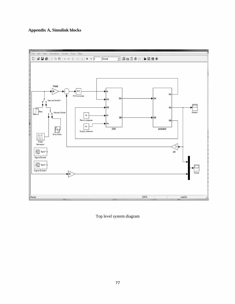
77

Appendix A, Simulink blocks

Top level system diagram

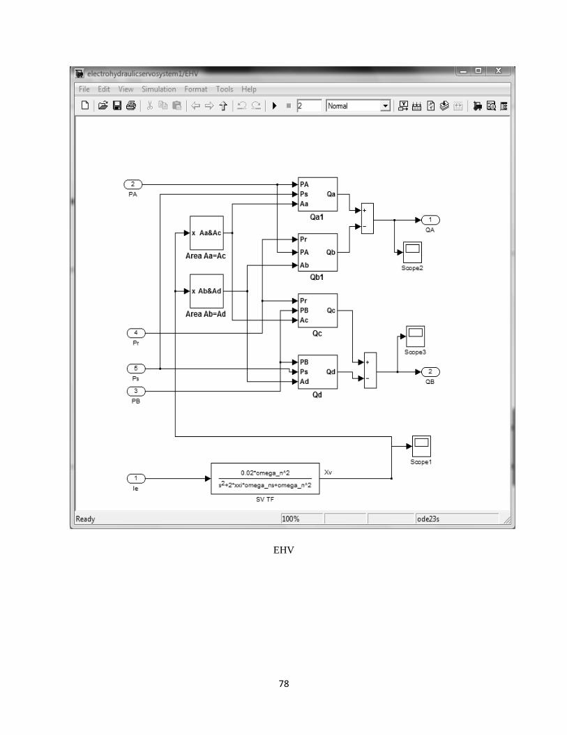
78

EHV

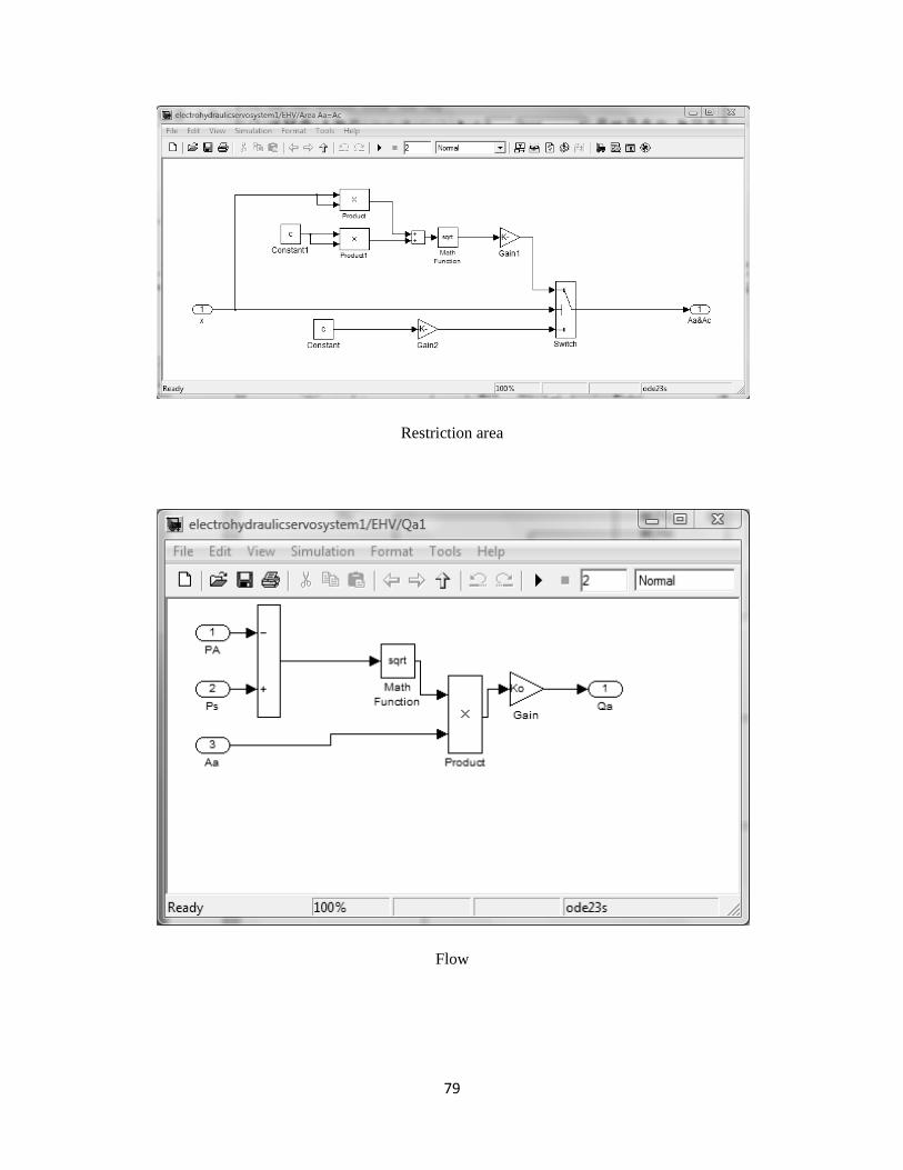
79

Restriction area

Flow

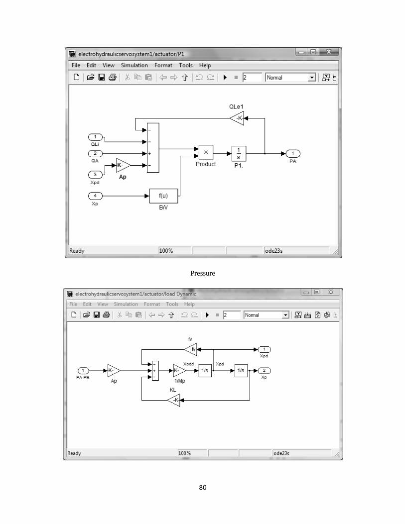
80

Pressure

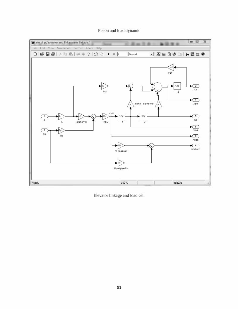
81

Piston and load dynamic

Elevator linkage and load cell

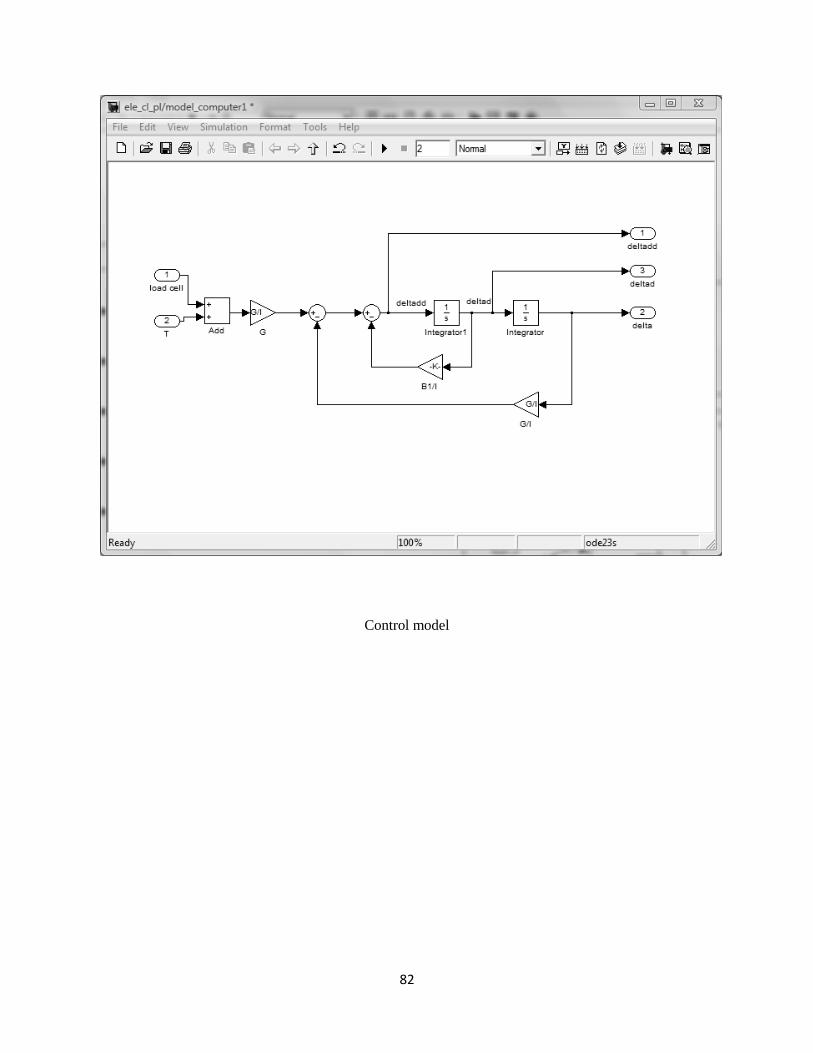
82

Control model

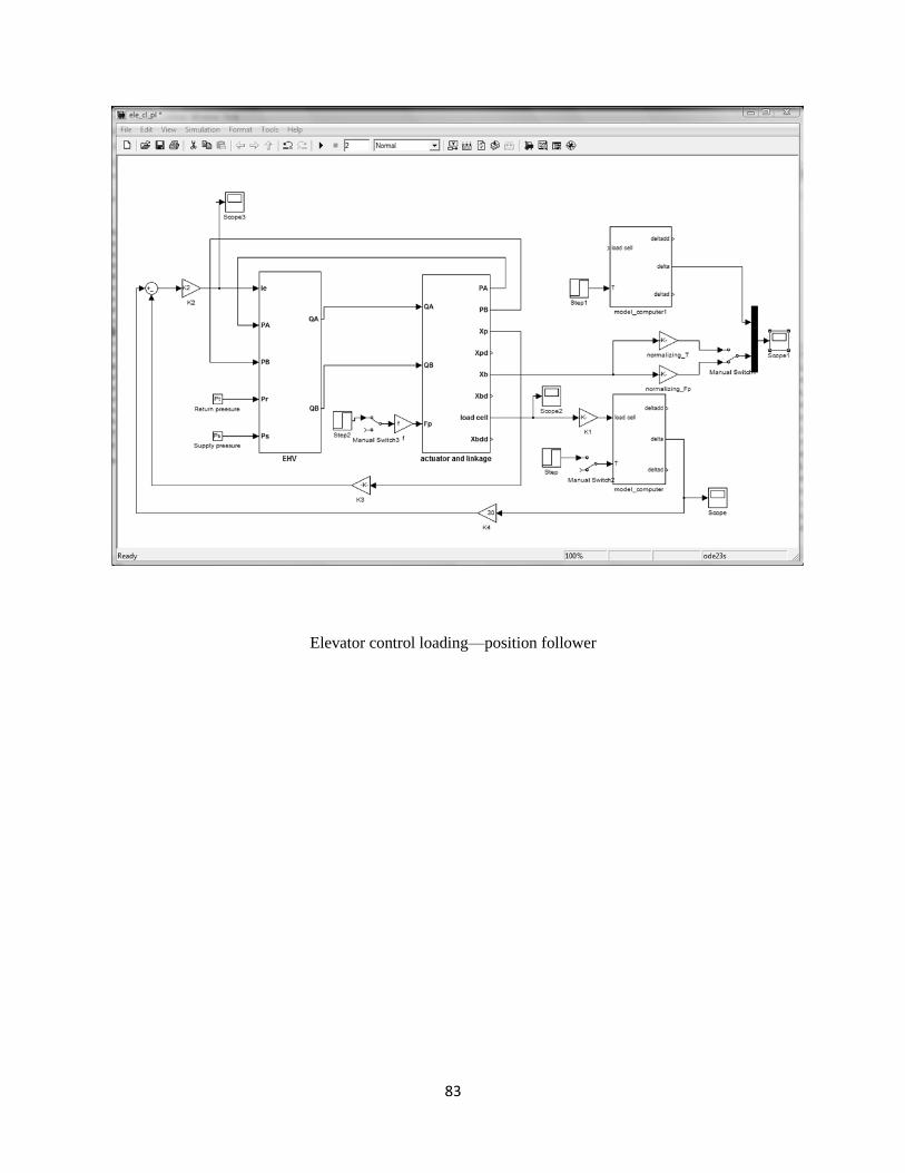
83

Elevator control loading—position follower

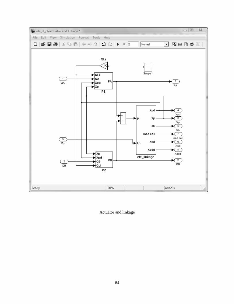
84

Actuator and linkage

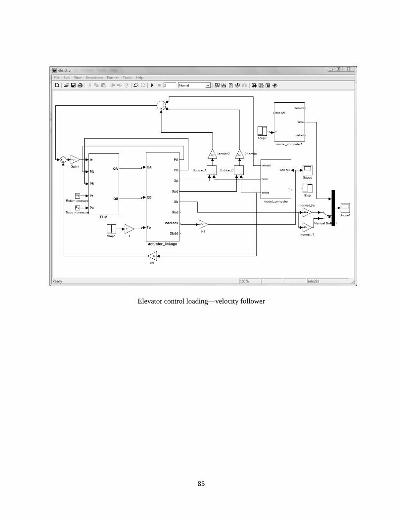
85

Elevator control loading—velocity follower

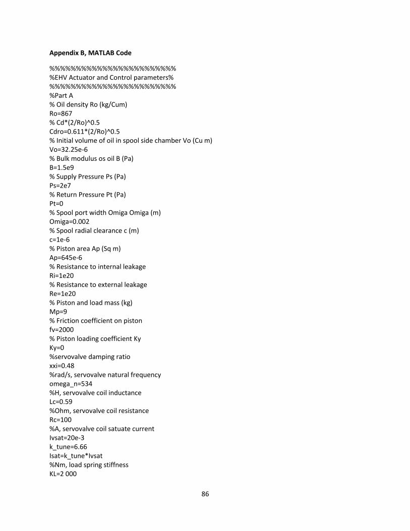
86

Appendix B, MATLAB Code

%%%%%%%%%%%%%%%%%%%%%%%% %EHV Actuator and Control parameters% %%%%%%%%%%%%%%%%%%%%%%%% %Part A % Oil density Ro (kg/Cum) Ro=867 % Cd*(2/Ro)^0.5 Cdro=0.611*(2/Ro)^0.5 % Initial volume of oil in spool side chamber Vo (Cu m) Vo=32.25e-6 % Bulk modulus os oil B (Pa) B=1.5e9 % Supply Pressure Ps (Pa) Ps=2e7 % Return Pressure Pt (Pa) Pt=0 % Spool port width Omiga Omiga (m) Omiga=0.002 % Spool radial clearance c (m) c=1e-6 % Piston area Ap (Sq m) Ap=645e-6 % Resistance to internal leakage Ri=1e20 % Resistance to external leakage Re=1e20 % Piston and load mass (kg) Mp=9 % Friction coefficient on piston fv=2000 % Piston loading coefficient Ky Ky=0 %servovalve damping ratio xxi=0.48 %rad/s, servovalve natural frequency omega_n=534 %H, servovalve coil inductance Lc=0.59 %Ohm, servovalve coil resistance Rc=100 %A, servovalve coil satuate current Ivsat=20e-3 k_tune=6.66 Isat=k_tune*Ivsat %Nm, load spring stiffness KL=2 000

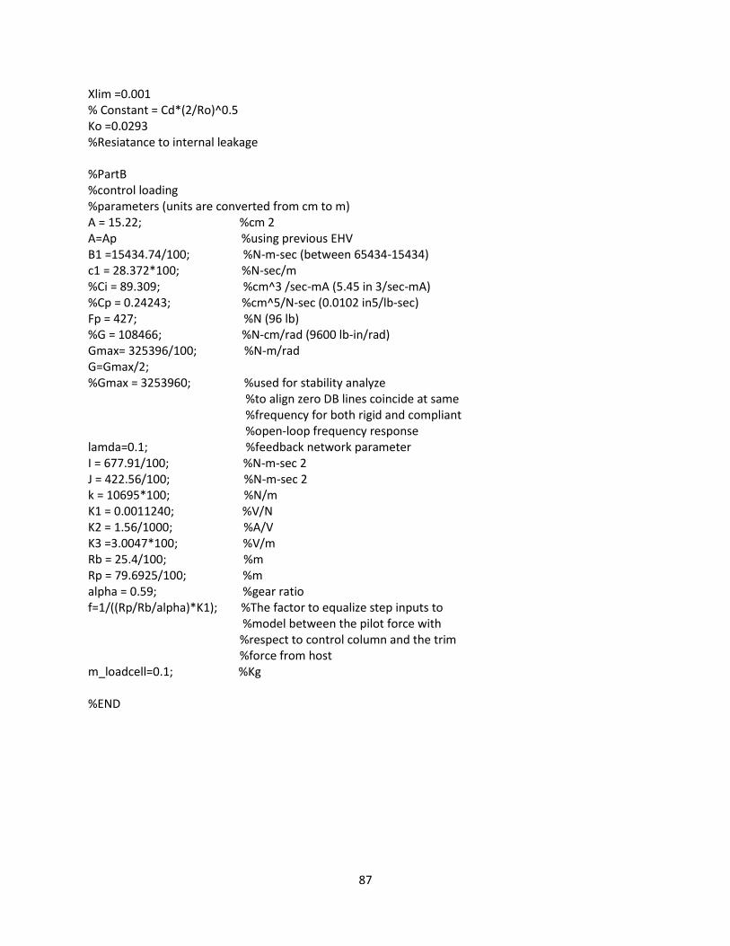
87

Xlim =0.001 % Constant = Cd*(2/Ro)^0.5 Ko =0.0293 %Resiatance to internal leakage %PartB %control loading %parameters (units are converted from cm to m) A = 15.22; %cm 2 A=Ap %using previous EHV B1 =15434.74/100; %N-m-sec (between 65434-15434) c1 = 28.372*100; %N-sec/m %Ci = 89.309; %cm^3 /sec-mA (5.45 in 3/sec-mA) %Cp = 0.24243; %cm^5/N-sec (0.0102 in5/lb-sec) Fp = 427; %N (96 lb) %G = 108466; %N-cm/rad (9600 lb-in/rad) Gmax= 325396/100; %N-m/rad G=Gmax/2; %Gmax = 3253960; %used for stability analyze %to align zero DB lines coincide at same %frequency for both rigid and compliant %open-loop frequency response lamda=0.1; %feedback network parameter I = 677.91/100; %N-m-sec 2 J = 422.56/100; %N-m-sec 2 k = 10695*100; %N/m K1 = 0.0011240; %V/N K2 = 1.56/1000; %A/V K3 =3.0047*100; %V/m Rb = 25.4/100; %m Rp = 79.6925/100; %m alpha = 0.59; %gear ratio f=1/((Rp/Rb/alpha)*K1); %The factor to equalize step inputs to %model between the pilot force with %respect to control column and the trim %force from host m_loadcell=0.1; %Kg %END

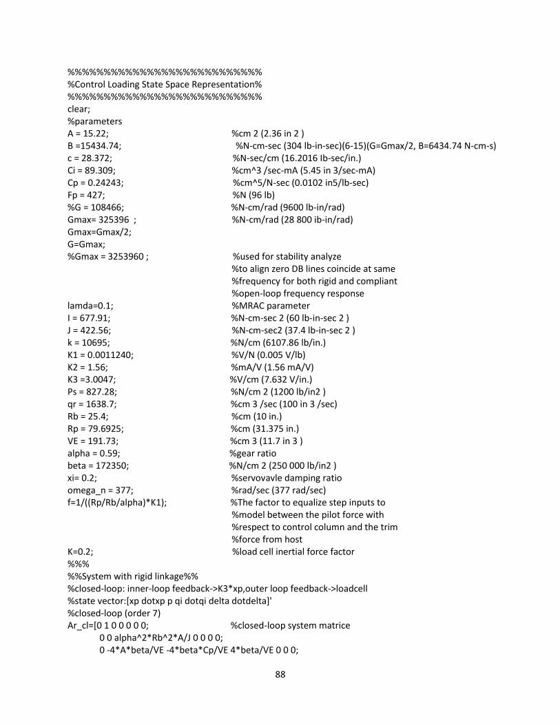
88

%%%%%%%%%%%%%%%%%%%%%%%%%%% %Control Loading State Space Representation% %%%%%%%%%%%%%%%%%%%%%%%%%%% clear; %parameters A = 15.22; %cm 2 (2.36 in 2 ) B =15434.74; %N-cm-sec (304 lb-in-sec)(6-15)(G=Gmax/2, B=6434.74 N-cm-s) c = 28.372; %N-sec/cm (16.2016 Ib-sec/in.) Ci = 89.309; %cm^3 /sec-mA (5.45 in 3/sec-mA) Cp = 0.24243; %cm^5/N-sec (0.0102 in5/lb-sec) Fp = 427; %N (96 lb) %G = 108466; %N-cm/rad (9600 lb-in/rad) Gmax= 325396 ; %N-cm/rad (28 800 ib-in/rad) Gmax=Gmax/2; G=Gmax; %Gmax = 3253960 ; %used for stability analyze %to align zero DB lines coincide at same %frequency for both rigid and compliant %open-loop frequency response lamda=0.1; %MRAC parameter I = 677.91; %N-cm-sec 2 (60 lb-in-sec 2 ) J = 422.56; %N-cm-sec2 (37.4 lb-in-sec 2 ) k = 10695; %N/cm (6107.86 lb/in.) K1 = 0.0011240; %V/N (0.005 V/lb) K2 = 1.56; %mA/V (1.56 mA/V) K3 =3.0047; %V/cm (7.632 V/in.) Ps = 827.28; %N/cm 2 (1200 lb/in2 ) qr = 1638.7; %cm 3 /sec (100 in 3 /sec) Rb = 25.4; %cm (10 in.) Rp = 79.6925; %cm (31.375 in.) VE = 191.73; %cm 3 (11.7 in 3 ) alpha = 0.59; %gear ratio beta = 172350; %N/cm 2 (250 000 lb/in2 ) xi= 0.2; %servovavle damping ratio omega_n = 377; %rad/sec (377 rad/sec) f=1/((Rp/Rb/alpha)*K1); %The factor to equalize step inputs to %model between the pilot force with %respect to control column and the trim %force from host K=0.2; %load cell inertial force factor %%% %%System with rigid linkage%% %closed-loop: inner-loop feedback->K3*xp,outer loop feedback->loadcell %state vector:[xp dotxp p qi dotqi delta dotdelta]' %closed-loop (order 7) Ar_cl=[0 1 0 0 0 0 0; %closed-loop system matrice 0 0 alpha^2*Rb^2*A/J 0 0 0 0; 0 -4*A*beta/VE -4*beta*Cp/VE 4*beta/VE 0 0 0;

89

0 0 0 0 1 0 0; -Ci*omega_n^2*K2*K3 0 0 -omega_n^2 -2*xi*omega_n Ci*omega_n^2*K2 0; 0 0 0 0 0 0 1; 0 0 -K*K1*G*A/I 0 0 -G/I -B/I]; Br_cl_Fp=f*[0 alpha*Rb*Rp/J 0 0 0 0 (1-K)*(Rp/Rb/alpha)*K1*G/I]'; %input Br_cl_F=f*[0 0 0 0 0 0 0; %n x n form 0 0 0 0 0 0 alpha*Rb*Rp/J; 0 0 0 0 0 0 0; 0 0 0 0 0 0 0; 0 0 0 0 0 0 0; 0 0 0 0 0 0 0; 0 0 0 0 0 0 (1-K)*(Rp/Rb/alpha)*K1*G/I]; Br_cl_T=[0 0 0 0 0 0 G/I]'; %input trim force Cr_cl_xb=[1/alpha/0.62 0 0 0 0 0 0]; %output xb. normalized divider: %0.56 fot T input %0.62 for Fp input Cr_cl_Ap=[0 0 A*K1 0 0 0 0]; %output Ap Cr_cl_T_loadcell=[0 0 -0.1*A*K1 0 0 0 0]; %m_loadcell=0.1 Cr_cl_Fp_loadcell=[0 0 -K*A*K1 0 0 0 0]; Dr_cl_Fp_loadcell=[0 0 0 0 0 0 f*(1-K)*(Rp/Rb/alpha)*K1]; D=zeros; %Fp %closed-loop (Fp-->xb) r_cl_Fp_xb=ss(Ar_cl,Br_cl_Fp,Cr_cl_xb,D); %closed-loop (Fp-->Ap) r_cl_Fp_Ap=ss(Ar_cl,Br_cl_F,Cr_cl_Ap,D); %closed-loop (Fp-->loadcell) r_cl_Fp_loadcell=ss(Ar_cl,Br_cl_F,Cr_cl_Fp_loadcell,Dr_cl_Fp_loadcell); %T %closed-loop (T-->xp) r_cl_T_xb=ss(Ar_cl,Br_cl_T,Cr_cl_xb,D); %closed-loop (T-->Ap) r_cl_T_Ap=ss(Ar_cl,Br_cl_T,Cr_cl_Ap,D); %closed-loop (T-->loadcell) r_cl_T_loadcell=ss(Ar_cl,Br_cl_T,Cr_cl_T_loadcell,D) %open loop(delta), eT input,i=K2*Ci*(eT-K3*xp) +f*(1-K)*(Rp/Rb/alpha)*K1) %state vector:[xp dotxp p qi dotqi delta dotdelta]' %rank(Ar_op)=7 Ar_op=[0 1 0 0 0 0 0; %open loop system matrice 0 0 alpha^2*Rb^2*A/J 0 0 0 0; 0 -4*A*beta/VE -4*beta*Cp/VE 4*beta/VE 0 0 0; 0 0 0 0 1 0 0; -Ci*omega_n^2*K2*K3 0 0 -omega_n^2 -2*xi*omega_n 0 0; 0 0 0 0 0 0 1; 0 0 K1*Gmax*A/I 0 0 -G/I -B/I]; Br_op_eT= [0 0 0 0 Ci*omega_n^2*K2 0 0]'; %input eT Cr_op_del=[0 0 0 0 0 1 0]; %output delta

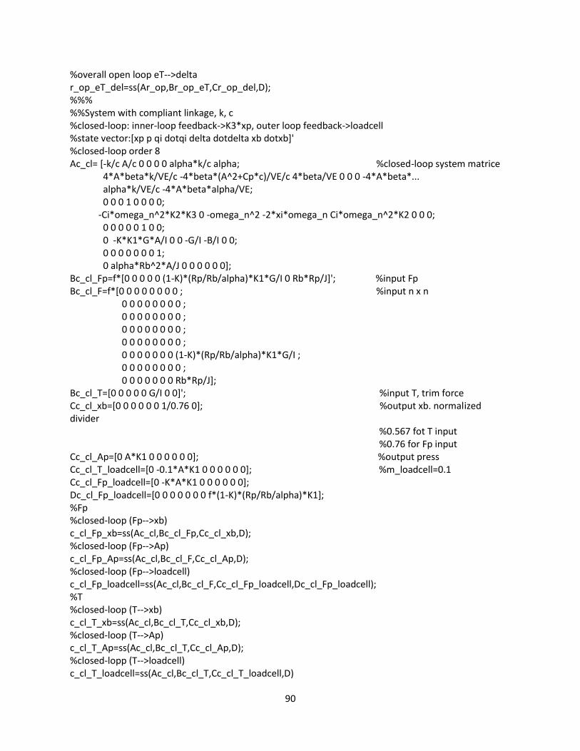
90

%overall open loop eT-->delta r_op_eT_del=ss(Ar_op,Br_op_eT,Cr_op_del,D); %%% %%System with compliant linkage, k, c %closed-loop: inner-loop feedback->K3*xp, outer loop feedback->loadcell %state vector:[xp p qi dotqi delta dotdelta xb dotxb]' %closed-loop order 8 Ac_cl= [-k/c A/c 0 0 0 0 alpha*k/c alpha; %closed-loop system matrice 4*A*beta*k/VE/c -4*beta*(A^2+Cp*c)/VE/c 4*beta/VE 0 0 0 -4*A*beta*... alpha*k/VE/c -4*A*beta*alpha/VE; 0 0 0 1 0 0 0 0; -Ci*omega_n^2*K2*K3 0 -omega_n^2 -2*xi*omega_n Ci*omega_n^2*K2 0 0 0; 0 0 0 0 0 1 0 0; 0 -K*K1*G*A/I 0 0 -G/I -B/I 0 0; 0 0 0 0 0 0 0 1; 0 alpha*Rb^2*A/J 0 0 0 0 0 0]; Bc_cl_Fp=f*[0 0 0 0 0 (1-K)*(Rp/Rb/alpha)*K1*G/I 0 Rb*Rp/J]'; %input Fp Bc_cl_F=f*[0 0 0 0 0 0 0 0 ; %input n x n 0 0 0 0 0 0 0 0 ; 0 0 0 0 0 0 0 0 ; 0 0 0 0 0 0 0 0 ; 0 0 0 0 0 0 0 0 ; 0 0 0 0 0 0 0 (1-K)*(Rp/Rb/alpha)*K1*G/I ; 0 0 0 0 0 0 0 0 ; 0 0 0 0 0 0 0 Rb*Rp/J]; Bc_cl_T=[0 0 0 0 0 G/I 0 0]'; %input T, trim force Cc_cl_xb=[0 0 0 0 0 0 1/0.76 0]; %output xb. normalized divider %0.567 fot T input %0.76 for Fp input Cc_cl_Ap=[0 A*K1 0 0 0 0 0 0]; %output press Cc_cl_T_loadcell=[0 -0.1*A*K1 0 0 0 0 0 0]; %m_loadcell=0.1 Cc_cl_Fp_loadcell=[0 -K*A*K1 0 0 0 0 0 0]; Dc_cl_Fp_loadcell=[0 0 0 0 0 0 0 f*(1-K)*(Rp/Rb/alpha)*K1]; %Fp %closed-loop (Fp-->xb) c_cl_Fp_xb=ss(Ac_cl,Bc_cl_Fp,Cc_cl_xb,D); %closed-loop (Fp-->Ap) c_cl_Fp_Ap=ss(Ac_cl,Bc_cl_F,Cc_cl_Ap,D); %closed-loop (Fp-->loadcell) c_cl_Fp_loadcell=ss(Ac_cl,Bc_cl_F,Cc_cl_Fp_loadcell,Dc_cl_Fp_loadcell); %T %closed-loop (T-->xb) c_cl_T_xb=ss(Ac_cl,Bc_cl_T,Cc_cl_xb,D); %closed-loop (T-->Ap) c_cl_T_Ap=ss(Ac_cl,Bc_cl_T,Cc_cl_Ap,D); %closed-lopp (T-->loadcell) c_cl_T_loadcell=ss(Ac_cl,Bc_cl_T,Cc_cl_T_loadcell,D)

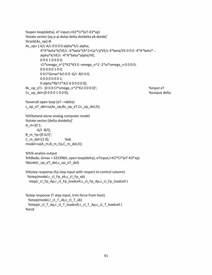
91

%open loop(delta), eT input,i=K2*Ci*(eT-K3*xp) %state vector:[xp p qi dotqi delta dotdelta xb dotxb]' %rank(Ac_op)=8 Ac_op= [-k/c A/c 0 0 0 0 alpha*k/c alpha; 4*A*beta*k/VE/c -4*beta*(A^2+Cp*c)/VE/c 4*beta/VE 0 0 0 -4*A*beta*... alpha*k/VE/c -4*A*beta*alpha/VE; 0 0 0 1 0 0 0 0; -Ci*omega_n^2*K2*K3 0 -omega_n^2 -2*xi*omega_n 0 0 0 0; 0 0 0 0 0 1 0 0; 0 K1*Gmax*A/I 0 0 -G/I -B/I 0 0; 0 0 0 0 0 0 0 1; 0 alpha*Rb^2*A/J 0 0 0 0 0 0]; Bc_op_eT= [0 0 0 Ci*omega_n^2*K2 0 0 0 0]'; %input eT Cc_op_del=[0 0 0 0 1 0 0 0]; %output delta %overall open loop (eT-->delta) c_op_eT_del=ss(Ac_op,Bc_op_eT,Cc_op_del,D); %%%stand alone analog computer model %state vector:[delta dotdelta]' A_m=[0 1; -G/I -B/I]; B_m_Fp=[0 G/I]'; C_m_del=[1 0]; %xb model=ss(A_m,B_m_Fp,C_m_del,D); %%% analize output %%Bode, Gmax = 3253960, open loop(delta), eTinput,i=K2*Ci*(eT-K3*xp) %bode(r_op_eT_del,c_op_eT_del) %%step response (Fp step input with respect to control column) %step(model,r_cl_Fp_xb,c_cl_Fp_xb) step(r_cl_Fp_Ap,r_cl_Fp_loadcell,c_cl_Fp_Ap,c_cl_Fp_loadcell ) %step response (T step input, trim force from host) %step(model,r_cl_T_xb,c_cl_T_xb) %step(r_cl_T_Ap,r_cl_T_loadcell,c_cl_T_Ap,c_cl_T_loadcell ) %end