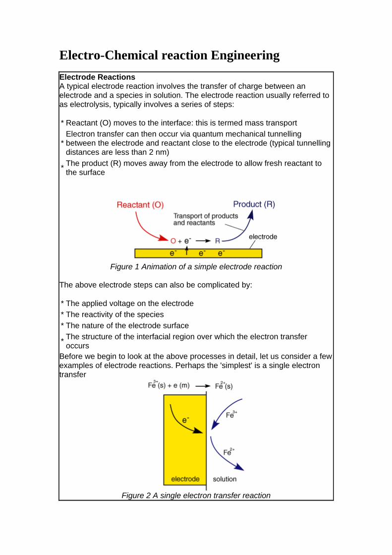
Electro-Chemical reaction Engineering Electrode Reactions A typical electrode reaction involves the transfer of charge between an electrode and a species in solution. The electrode reaction usually referred to as electrolysis, typically involves a series of steps:

* Reactant (O) moves to the interface: this is termed mass transport

* Electron transfer can then occur via quantum mechanical tunnelling between the electrode and reactant close to the electrode (typical tunnelling distances are less than 2 nm)

* The product (R) moves away from the electrode to allow fresh reactant to the surface

Figure 1 Animation of a simple electrode reaction

The above electrode steps can also be complicated by:

* The applied voltage on the electrode * The reactivity of the species * The nature of the electrode surface

* The structure of the interfacial region over which the electron transfer occurs

Before we begin to look at the above processes in detail, let us consider a few examples of electrode reactions. Perhaps the 'simplest' is a single electron transfer

Figure 2 A single electron transfer reaction

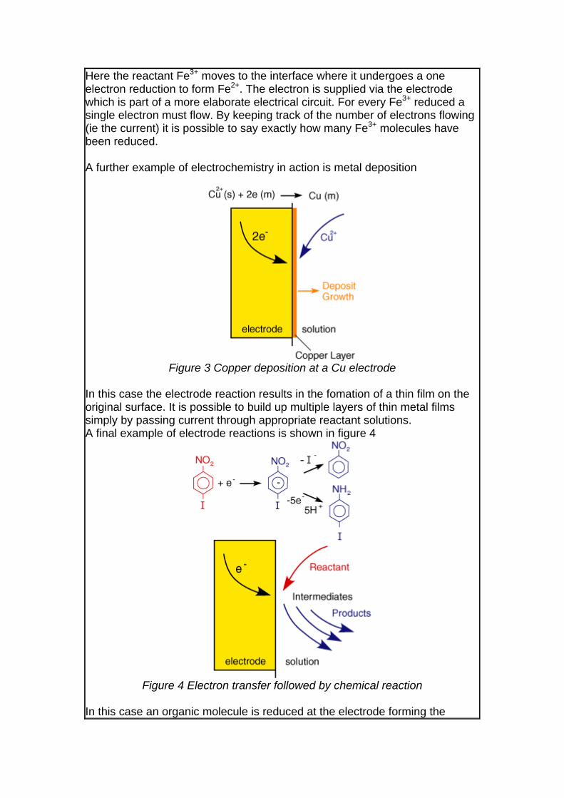
Here the reactant Fe3+ moves to the interface where it undergoes a one electron reduction to form Fe2+. The electron is supplied via the electrode which is part of a more elaborate electrical circuit. For every Fe3+ reduced a single electron must flow. By keeping track of the number of electrons flowing (ie the current) it is possible to say exactly how many Fe3+ molecules have been reduced. A further example of electrochemistry in action is metal deposition

Figure 3 Copper deposition at a Cu electrode

In this case the electrode reaction results in the fomation of a thin film on the original surface. It is possible to build up multiple layers of thin metal films simply by passing current through appropriate reactant solutions. A final example of electrode reactions is shown in figure 4

Figure 4 Electron transfer followed by chemical reaction

In this case an organic molecule is reduced at the electrode forming the

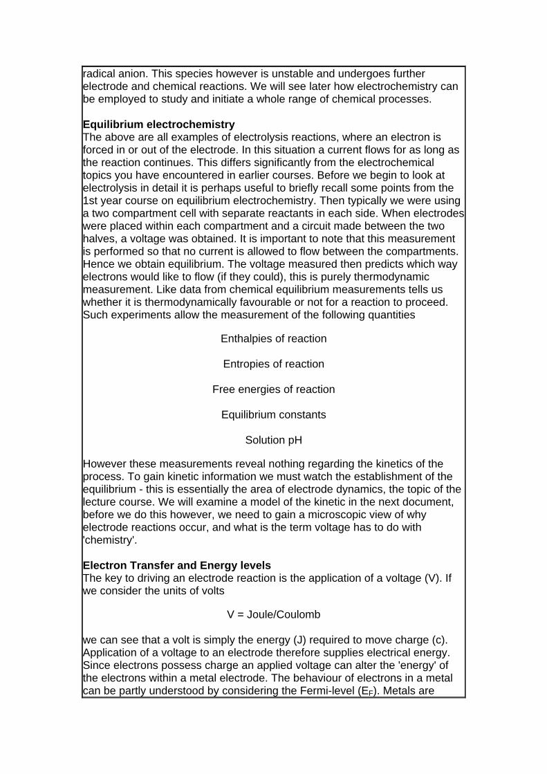
radical anion. This species however is unstable and undergoes further electrode and chemical reactions. We will see later how electrochemistry can be employed to study and initiate a whole range of chemical processes. Equilibrium electrochemistry The above are all examples of electrolysis reactions, where an electron is forced in or out of the electrode. In this situation a current flows for as long as the reaction continues. This differs significantly from the electrochemical topics you have encountered in earlier courses. Before we begin to look at electrolysis in detail it is perhaps useful to briefly recall some points from the 1st year course on equilibrium electrochemistry. Then typically we were using a two compartment cell with separate reactants in each side. When electrodes were placed within each compartment and a circuit made between the two halves, a voltage was obtained. It is important to note that this measurement is performed so that no current is allowed to flow between the compartments. Hence we obtain equilibrium. The voltage measured then predicts which way electrons would like to flow (if they could), this is purely thermodynamic measurement. Like data from chemical equilibrium measurements tells us whether it is thermodynamically favourable or not for a reaction to proceed. Such experiments allow the measurement of the following quantities

Enthalpies of reaction

Entropies of reaction

Free energies of reaction

Equilibrium constants

Solution pH

However these measurements reveal nothing regarding the kinetics of the process. To gain kinetic information we must watch the establishment of the equilibrium - this is essentially the area of electrode dynamics, the topic of the lecture course. We will examine a model of the kinetic in the next document, before we do this however, we need to gain a microscopic view of why electrode reactions occur, and what is the term voltage has to do with 'chemistry'. Electron Transfer and Energy levels The key to driving an electrode reaction is the application of a voltage (V). If we consider the units of volts

V = Joule/Coulomb we can see that a volt is simply the energy (J) required to move charge (c). Application of a voltage to an electrode therefore supplies electrical energy. Since electrons possess charge an applied voltage can alter the 'energy' of the electrons within a metal electrode. The behaviour of electrons in a metal can be partly understood by considering the Fermi-level (EF). Metals are

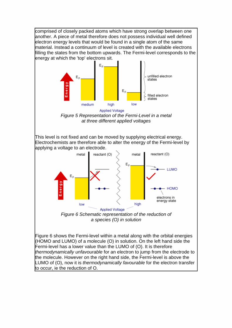
comprised of closely packed atoms which have strong overlap between one another. A piece of metal therefore does not possess individual well defined electron energy levels that would be found in a single atom of the same material. Instead a continuum of level is created with the available electrons filling the states from the bottom upwards. The Fermi-level corresponds to the energy at which the 'top' electrons sit.

Figure 5 Representation of the Fermi-Level in a metal

at three different applied voltages This level is not fixed and can be moved by supplying electrical energy. Electrochemists are therefore able to alter the energy of the Fermi-level by applying a voltage to an electrode.

Figure 6 Schematic representation of the reduction of

a species (O) in solution Figure 6 shows the Fermi-level within a metal along with the orbital energies (HOMO and LUMO) of a molecule (O) in solution. On the left hand side the Fermi-level has a lower value than the LUMO of (O). It is therefore thermodynamically unfavourable for an electron to jump from the electrode to the molecule. However on the right hand side, the Fermi-level is above the LUMO of (O), now it is thermodynamically favourable for the electron transfer to occur, ie the reduction of O.

Figure 7 Animation of the reduction of

a species (O) in solution Whether the process occurs depends upon the rate (kinetics) of the electron transfer reaction and the next document describes a model which explains this behaviour

Introduction As we have noted in the first section it is possible to transfer electrons between an electrode and a chemical species in solution. This process is called electrolysis and results in a reactant undergoing an oxidation or reduction reaction. Unlike equilibrium measurements recorded using a two electrode, two compartment cell, electrolysis results in the flow of current around an electrical circuit. This current can be controlled by a number of factors, the two most common are (i) the rate of electron transfer between the metal and species in solution and (ii) the transport of material to and from the electrode interface.

Kinetics of Electron Transfer In this section we will develop a quantitative model for the influence of the electrode voltage on the rate of electron transfer. For simplicity we will consider a single electron transfer reaction between two species (O) and (R)

The current flowing in either the reductive or oxidative steps can be predicted using the following expressions

For the reduction reaction the current (ic) is related to the electrode area (A), the surface concentration of the reactant [O]o, the rate constant for the

electron transfer (kRed or kOx) and Faraday's constant (F). A similar expression is valid for the oxidation, now the current is labeled (ia), with the surface concentration that of the species R. Similarly the rate constant for electron transfer corresponds to that of the oxidation process. Note that by definition the reductive current is negative and the oxidative positive, the difference in sign simply tells us that current flows in opposite directions across the interface depending upon whether we are studying an oxidation or reduction.To establish how the rate constants kOx and kRed are influenced by the applied voltage we will use transition state theory from chemical kinetics. You will recall that in this theory the reaction is considered to proceed via an energy barrier. The summit of this barrier is referred to as the transition state.

The rate of reaction for a chemical process (eg)

is predicted by an equation of the form

where the term in the exponential is the free energy change in taking the reactant from its initial value to the transition state divided by the temperature and gas constant. This free energy plot is also qualitatively valid for electrode reactions

where the free energy plot below corresponds to the thermodynamic response at a single fixed voltage.

Using this picture the activation free energy for the reduction and oxidation reactions are

and so the corresponding reaction rates are given by

So for a single applied voltage the free energy profiles appear qualitatively to be the same as corresponding chemical processes. However if we now plot a series of these free energy profiles as a function of voltage it is apparent that the plots alter as a function of the voltage. It is important to note that the left hand side of the figure corresponding to the free energy of R is invariant with voltage, whereas the right hand side ( O + e) shows a strong dependence.

At voltage V1 the formation of the species O is thermodynamically favoured.

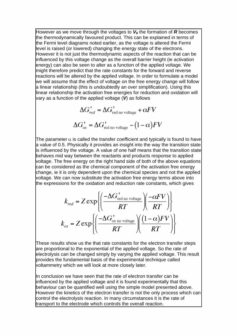
However as we move through the voltages to V6 the formation of R becomes the thermodynamically favoured product. This can be explained in terms of the Fermi level diagrams noted earlier, as the voltage is altered the Fermi level is raised (or lowered) changing the energy state of the electrons. However it is not just the thermodynamic aspects of the reaction that can be influenced by this voltage change as the overall barrier height (ie activation energy) can also be seen to alter as a function of the applied voltage. We might therefore predict that the rate constants for the forward and reverse reactions will be altered by the applied voltage. In order to formulate a model we will assume that the effect of voltage on the free energy change will follow a linear relationship (this is undoubtedly an over simplification). Using this linear relationship the activation free energies for reduction and oxidation will vary as a function of the applied voltage (V) as follows

The parameter α is called the transfer coefficient and typically is found to have a value of 0.5. Physically it provides an insight into the way the transition state is influenced by the voltage. A value of one half means that the transition state behaves mid way between the reactants and products response to applied voltage. The free energy on the right hand side of both of the above equations can be considered as the chemical component of the activation free energy change, ie it is only dependent upon the chemical species and not the applied voltage. We can now substitute the activation free energy terms above into the expressions for the oxidation and reduction rate constants, which gives

These results show us the that rate constants for the electron transfer steps are proportional to the exponential of the applied voltage. So the rate of electrolysis can be changed simply by varying the applied voltage. This result provides the fundamental basis of the experimental technique called voltammetry which we will look at more closely later. In conclusion we have seen that the rate of electron transfer can be influenced by the applied voltage and it is found experimentally that this behaviour can be quantified well using the simple model presented above. However the kinetics of the electron transfer is not the only process which can control the electrolysis reaction. In many circumstances it is the rate of transport to the electrode which controls the overall reaction.

Introduction In this section two closely related forms of voltammetry are introduced

* Linear Sweep Voltammetry * Cyclic Voltammetry

We shall see how these measurements can be employed to study the electron transfer kinetics and transport properties of electrolysis reactions.

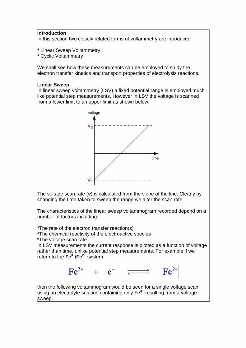
Linear Sweep In linear sweep voltammetry (LSV) a fixed potential range is employed much like potential step measurements. However in LSV the voltage is scanned from a lower limit to an upper limit as shown below.

The voltage scan rate (v) is calculated from the slope of the line. Clearly by changing the time taken to sweep the range we alter the scan rate.

The characteristics of the linear sweep voltammogram recorded depend on a number of factors including:

*The rate of the electron transfer reaction(s) *The chemical reactivity of the electroactive species *The voltage scan rate In LSV measurements the current response is plotted as a function of voltage rather than time, unlike potential step measurements. For example if we return to the Fe3+/Fe2+ system

then the following voltammogram would be seen for a single voltage scan using an electrolyte solution containing only Fe3+ resulting from a voltage sweep.

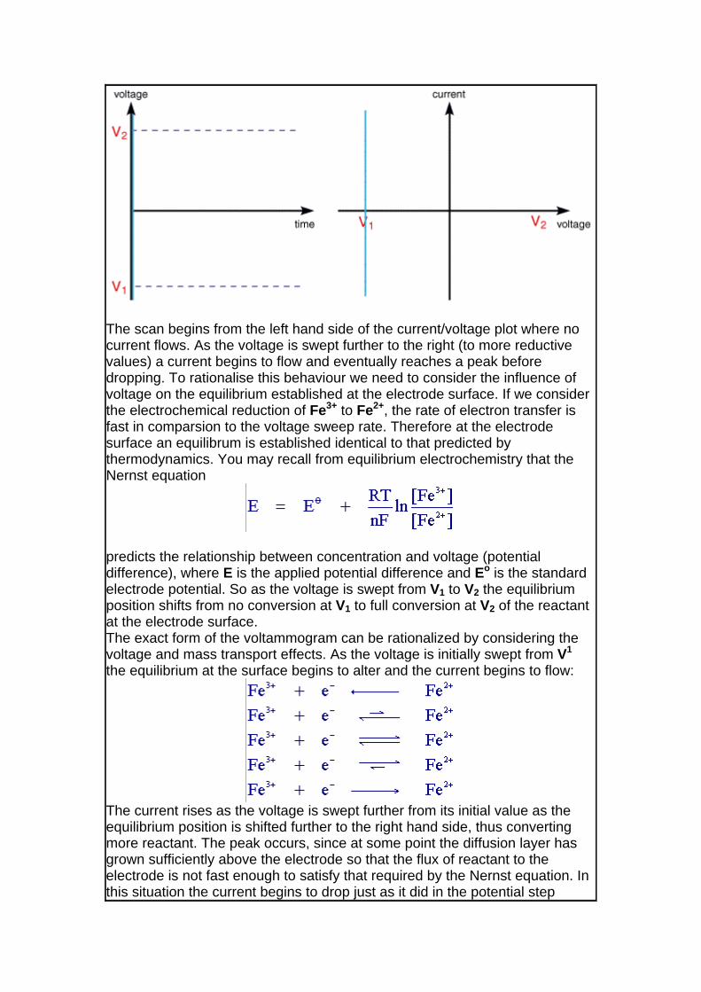
The scan begins from the left hand side of the current/voltage plot where no current flows. As the voltage is swept further to the right (to more reductive values) a current begins to flow and eventually reaches a peak before dropping. To rationalise this behaviour we need to consider the influence of voltage on the equilibrium established at the electrode surface. If we consider the electrochemical reduction of Fe3+ to Fe2+, the rate of electron transfer is fast in comparsion to the voltage sweep rate. Therefore at the electrode surface an equilibrum is established identical to that predicted by thermodynamics. You may recall from equilibrium electrochemistry that the Nernst equation

predicts the relationship between concentration and voltage (potential difference), where E is the applied potential difference and Eo is the standard electrode potential. So as the voltage is swept from V1 to V2 the equilibrium position shifts from no conversion at V1 to full conversion at V2 of the reactant at the electrode surface. The exact form of the voltammogram can be rationalized by considering the voltage and mass transport effects. As the voltage is initially swept from V1 the equilibrium at the surface begins to alter and the current begins to flow:

The current rises as the voltage is swept further from its initial value as the equilibrium position is shifted further to the right hand side, thus converting more reactant. The peak occurs, since at some point the diffusion layer has grown sufficiently above the electrode so that the flux of reactant to the electrode is not fast enough to satisfy that required by the Nernst equation. In this situation the current begins to drop just as it did in the potential step

measurements. In fact the drop in current follows the same behaviour as that predicted by the Cottrell equation.

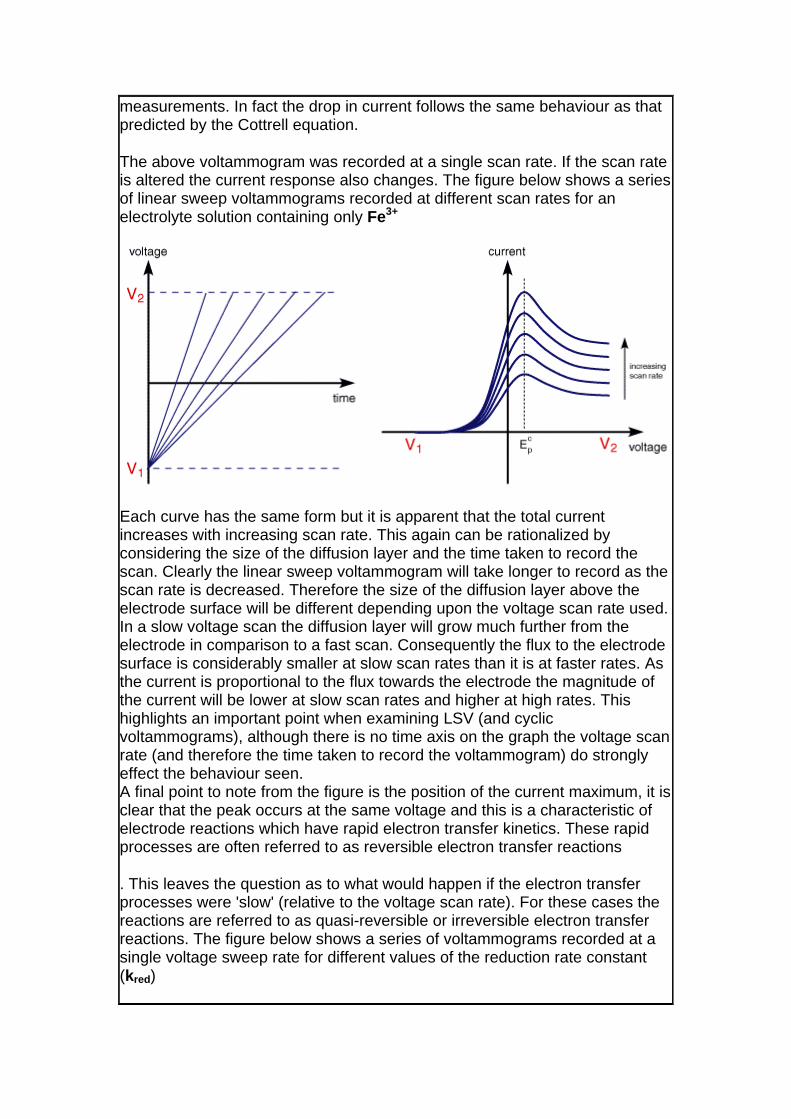
The above voltammogram was recorded at a single scan rate. If the scan rate is altered the current response also changes. The figure below shows a series of linear sweep voltammograms recorded at different scan rates for an electrolyte solution containing only Fe3+

Each curve has the same form but it is apparent that the total current increases with increasing scan rate. This again can be rationalized by considering the size of the diffusion layer and the time taken to record the scan. Clearly the linear sweep voltammogram will take longer to record as the scan rate is decreased. Therefore the size of the diffusion layer above the electrode surface will be different depending upon the voltage scan rate used. In a slow voltage scan the diffusion layer will grow much further from the electrode in comparison to a fast scan. Consequently the flux to the electrode surface is considerably smaller at slow scan rates than it is at faster rates. As the current is proportional to the flux towards the electrode the magnitude of the current will be lower at slow scan rates and higher at high rates. This highlights an important point when examining LSV (and cyclic voltammograms), although there is no time axis on the graph the voltage scan rate (and therefore the time taken to record the voltammogram) do strongly effect the behaviour seen. A final point to note from the figure is the position of the current maximum, it is clear that the peak occurs at the same voltage and this is a characteristic of electrode reactions which have rapid electron transfer kinetics. These rapid processes are often referred to as reversible electron transfer reactions

. This leaves the question as to what would happen if the electron transfer processes were 'slow' (relative to the voltage scan rate). For these cases the reactions are referred to as quasi-reversible or irreversible electron transfer reactions. The figure below shows a series of voltammograms recorded at a single voltage sweep rate for different values of the reduction rate constant (kred)

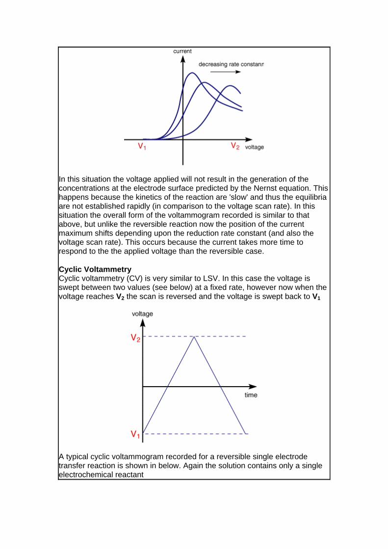
In this situation the voltage applied will not result in the generation of the concentrations at the electrode surface predicted by the Nernst equation. Thishappens because the kinetics of the reaction are 'slow' and thus the equilibria are not established rapidly (in comparison to the voltage scan rate). In this situation the overall form of the voltammogram recorded is similar to that above, but unlike the reversible reaction now the position of the current maximum shifts depending upon the reduction rate constant (and also the voltage scan rate). This occurs because the current takes more time to respond to the the applied voltage than the reversible case.

Cyclic Voltammetry Cyclic voltammetry (CV) is very similar to LSV. In this case the voltage is swept between two values (see below) at a fixed rate, however now when the voltage reaches V2 the scan is reversed and the voltage is swept back to V1

A typical cyclic voltammogram recorded for a reversible single electrode transfer reaction is shown in below. Again the solution contains only a single electrochemical reactant

The forward sweep produces an identical response to that seen for the LSV experiment. When the scan is reversed we simply move back through the equilibrium positions gradually converting electrolysis product (F2+ back to reactant (Fe3+). The current flow is now from the solution species back to the electrode and so occurs in the opposite sense to the forward seep but otherwise the behaviour can be explained in an identical manner. For a reversible electrochemical reaction the CV recorded has certain well defined characteristics.

I) The voltage separation between the current peaks is

II) The positions of peak voltage do not alter as a function of voltage scan rateIII) The ratio of the peak currents is equal to one

IV) The peak currents are proportional to the square root of the scan rate

The influence of the voltage scan rate on the current for a reversible electron transfer can be seen below

As with LSV the influence of scan rate is explained for a reversible electron transfer reaction in terms of the diffusion layer thickness. The CV for cases where the electron transfer is not reversible show considerably different behaviour from their reversible counterparts. The figure below shows the voltammogram for a quasi-reversible reaction for different values of the reduction and oxidation rate constants.

The first curve shows the case where both the oxidation and reduction rate constants are still fast, however, as the rate constants are lowered the curves shift to more reductive potentials. Again this may be rationalized in terms of the equilibrium at the surface is no longer establishing so rapidly. In these cases the peak separation is no longer fixed but varies as a function of the scan rate. Similarly the peak current no longer varies as a function of the square root of the scan rate.

By analysing the variation of peak position as a function of scan rate it is possible to gain an estimate for the electron transfer rate constants.

Introduction Cyclic voltammetry can be used to investigate the chemical reactivity of species. To illustrate this let us consider a few possible reactions.

First consider the EC reaction:

The notation for electrolysis reactions was first proposed by Testa and Reinmuth with any electrode steps being labeled E and any chemical steps labeled C. Hence the above reaction is referred to as the EC reaction. The mass transport equations for this reaction when diffusional transport is dominant are

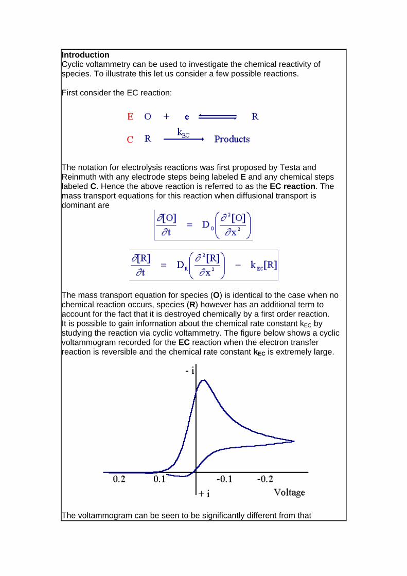
The mass transport equation for species (O) is identical to the case when no chemical reaction occurs, species (R) however has an additional term to account for the fact that it is destroyed chemically by a first order reaction. It is possible to gain information about the chemical rate constant kEC by studying the reaction via cyclic voltammetry. The figure below shows a cyclic voltammogram recorded for the EC reaction when the electron transfer reaction is reversible and the chemical rate constant kEC is extremely large.

The voltammogram can be seen to be significantly different from that

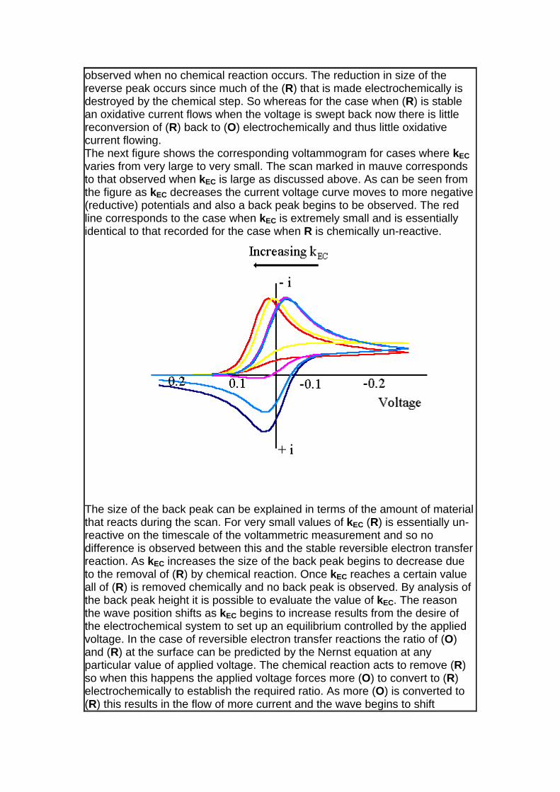
observed when no chemical reaction occurs. The reduction in size of the reverse peak occurs since much of the (R) that is made electrochemically is destroyed by the chemical step. So whereas for the case when (R) is stable an oxidative current flows when the voltage is swept back now there is little reconversion of (R) back to (O) electrochemically and thus little oxidative current flowing. The next figure shows the corresponding voltammogram for cases where kEC varies from very large to very small. The scan marked in mauve corresponds to that observed when kEC is large as discussed above. As can be seen from the figure as kEC decreases the current voltage curve moves to more negative (reductive) potentials and also a back peak begins to be observed. The red line corresponds to the case when kEC is extremely small and is essentially identical to that recorded for the case when R is chemically un-reactive.

The size of the back peak can be explained in terms of the amount of material that reacts during the scan. For very small values of kEC (R) is essentially un-reactive on the timescale of the voltammetric measurement and so no difference is observed between this and the stable reversible electron transfer reaction. As kEC increases the size of the back peak begins to decrease due to the removal of (R) by chemical reaction. Once kEC reaches a certain value all of (R) is removed chemically and no back peak is observed. By analysis of the back peak height it is possible to evaluate the value of kEC. The reason the wave position shifts as kEC begins to increase results from the desire of the electrochemical system to set up an equilibrium controlled by the applied voltage. In the case of reversible electron transfer reactions the ratio of (O) and (R) at the surface can be predicted by the Nernst equation at any particular value of applied voltage. The chemical reaction acts to remove (R) so when this happens the applied voltage forces more (O) to convert to (R) electrochemically to establish the required ratio. As more (O) is converted to (R) this results in the flow of more current and the wave begins to shift

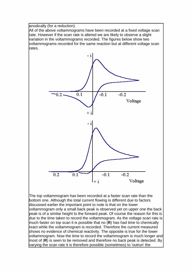
anodically (for a reduction). All of the above voltammograms have been recorded at a fixed voltage scan rate. However if the scan rate is altered we are likely to observe a slight variation in the voltammograms recorded. The figures below show two voltammograms recorded for the same reaction but at different voltage scan rates.

The top voltammogram has been recorded at a faster scan rate than the bottom one. Although the total current flowing is different due to factors discussed earlier the important point to note is that on the lower voltammogram only a small back peak is observed yet on upper one the back peak is of a similar height to the forward peak. Of course the reason for this is due to the time taken to record the voltammogram. As the voltage scan rate is much faster on top scan it is possible that no (R) has had time to chemically react while the voltammogram is recorded. Therefore the current measured shows no evidence of chemical reactivity. The opposite is true for the lower voltammogram. Now the time to record the voltammogram is much longer and most of (R) is seen to be removed and therefore no back peak is detected. By varying the scan rate it is therefore possible (sometimes) to 'outrun' the

chemical reaction. The EC mechanism is perhaps the simplest example of a coupled homogeneous chemical reaction. A slightly more complex case is the ECE reaction

The first step is similar to the EC process. However now the product for the chemical reaction (S) is also electrochemically active. The figure below shows the voltammogram for an ECE mechanism where the product (S) is more difficult to reduce than the starting material (O).

The scan starts from the left hand side and the first feature is the reduction of (O) to (R). However now if the scan is taken further a new peak is observed for the reduction of (S) to (T). On the reverse scan a back peak is seen for the (S/T) couple but only a small peak is observed for the (O/R) couple. Clearly for this reaction the chemical rate constant is 'fast' (compared to the voltage scan rate) and so almost all of (R) is removed by chemical reaction. Slightly different behaviour is seen if the product (S) is more easy to reduce:

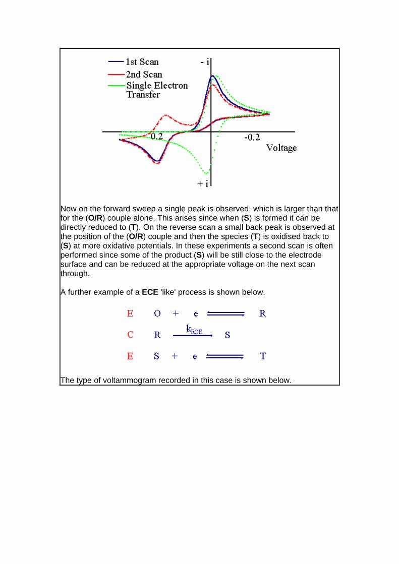
Now on the forward sweep a single peak is observed, which is larger than that for the (O/R) couple alone. This arises since when (S) is formed it can be directly reduced to (T). On the reverse scan a small back peak is observed at the position of the (O/R) couple and then the species (T) is oxidised back to (S) at more oxidative potentials. In these experiments a second scan is often performed since some of the product (S) will be still close to the electrode surface and can be reduced at the appropriate voltage on the next scan through.

A further example of a ECE 'like' process is shown below.

The type of voltammogram recorded in this case is shown below.

See if you can rationalize the behaviour here!

The final electrochemical mechanism we shall consider is a catalytic one

This reaction is referred to as the EC' mechanism. The prime (') on the C representing a catalytic process. In this case the chemical reaction regenerates the starting material (O). The figure below shows the corresponding cyclic voltammogram recorded for these types of reactions with different quantities of (Y) added to the solution

The current voltage curve with the lowest current corresponds to the case where no (Y) has been added to the solution and therefore no chemical

reaction occurs. However as (Y) is added the reaction can begin and for a fixed scan rate and concentration of (Y), the current will be higher than when no (Y) is present in solution. This of course is due to the fact that the reactant (O) is regenerated during the reaction and can therefore react again at the electrode surface. As the quantity of (Y) is increased the current also increases since more chemical reaction occurs. Fuel cell Introduction In this section we outline the key principles and processes occurring within a range of different fuel cells.

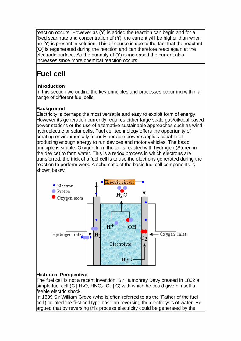
Background Electricity is perhaps the most versatile and easy to exploit form of energy. However its generation currently requires either large scale gas/oil/coal based power stations or the use of alternative sustainable approaches such as wind, hydroelectric or solar cells. Fuel cell technology offers the opportunity of creating environmentally friendly portable power supplies capable of producing enough energy to run devices and motor vehicles. The basic principle is simple: Oxygen from the air is reacted with hydrogen (Stored in the device) to form water. This is a redox process in which electrons are transferred, the trick of a fuel cell is to use the electrons generated during the reaction to perform work. A schematic of the basic fuel cell components is shown below

Historical Perspective The fuel cell is not a recent invention. Sir Humphrey Davy created in 1802 a simple fuel cell (C | H2O, HNO3| O2 | C) with which he could give himself a feeble electric shock. In 1839 Sir William Grove (who is often referred to as the 'Father of the fuel cell') created the first cell type base on reversing the electrolysis of water. He argued that by reversing this process electricity could be generated by the

reaction of hydrogen and oxygen together. Though the first fuel cell is nearly two centuries old, its development towards real world applications has been relatively slow. This is in part is due to the 'success' of the internal combustion engine which although inefficient, produces more than enough power for general applications in a range of industries. Another aspect holding back the successful application of fuel cells has also been the relatively complex materials science/chemistry which has to be optimised.

The term 'fuel cell' was first used by Ludwig Mond and Charles Langer in 1889, and this was followed by extensive work to try and develop usable devices. 1932 saw the first successful application of a fuel cell and this was demonstrated by Francis Bacon, By 1959 Bacon and coworkers demonstrated a 5KW system which was capable of powering welding machinery. Also around this period Harry Karl Ihrig demonstrated a 20 horse power tractor driven by Fuel cells. The 1960's saw a rapid expansion of research within the area, partly driven by funding from NASA who were looking for low weight, clean and highly efficient electricity sources for their space programme. An added bonus of the hydrogen fuel cell is the production of water (and heat) which was also extremely useful within their space craft.

In the period 1970-1990, Japanese companies also became a big investors in fuel cell research. By the 1980s Japan had small scale power stations operating and extensive interest from the automotive industry. For further details and links to a range of companies currently involved in fuel cell technology see: Construction and Applications of fuel cells

Operating Principles Fuel cells are often referred to as continuously operating batteries. They exploit electrolysis reactions in a similar manner to traditional batteries however the reagents are constantly resupplied to the cell and hence they do not become discharged like traditional batteries. An animation of the basic operation of a hydrogen fuel cell can be found at http://www.ballard.com/pem_animation.asp. In this case the two fuels are oxygen and hydrogen producing water (and heat) as the products. The hydrogen is fed to the 'fuel electrode' where it is oxidised into H+ ions. The oxygen is fed to the 'air electrode' where it is reduced to OH- ions through reaction with water in the electrolyte. Both those ions meet in the electrolyte between the two electrodes to form water. During this process, the electrons taken from the hydrogen are taken into a external electric circuit before returning to the cathode to form the OH- ions.

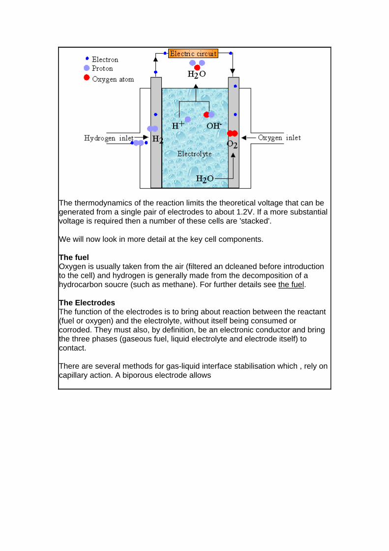
The thermodynamics of the reaction limits the theoretical voltage that can be generated from a single pair of electrodes to about 1.2V. If a more substantial voltage is required then a number of these cells are 'stacked'.

We will now look in more detail at the key cell components.

The fuel Oxygen is usually taken from the air (filtered an dcleaned before introduction to the cell) and hydrogen is generally made from the decomposition of a hydrocarbon soucre (such as methane). For further details see the fuel.

The Electrodes The function of the electrodes is to bring about reaction between the reactant (fuel or oxygen) and the electrolyte, without itself being consumed or corroded. They must also, by definition, be an electronic conductor and bring the three phases (gaseous fuel, liquid electrolyte and electrode itself) to contact.

There are several methods for gas-liquid interface stabilisation which , rely on capillary action. A biporous electrode allows

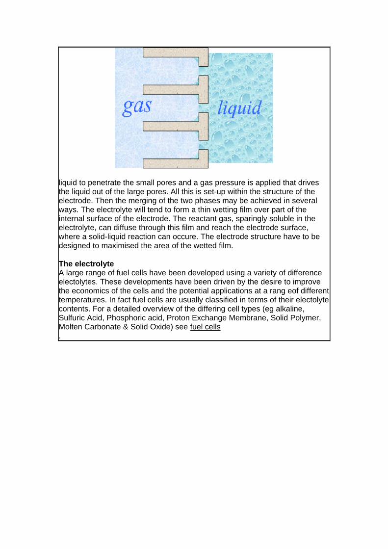
liquid to penetrate the small pores and a gas pressure is applied that drives the liquid out of the large pores. All this is set-up within the structure of the electrode. Then the merging of the two phases may be achieved in several ways. The electrolyte will tend to form a thin wetting film over part of the internal surface of the electrode. The reactant gas, sparingly soluble in the electrolyte, can diffuse through this film and reach the electrode surface, where a solid-liquid reaction can occure. The electrode structure have to be designed to maximised the area of the wetted film.

The electrolyte A large range of fuel cells have been developed using a variety of difference electolytes. These developments have been driven by the desire to improve the economics of the cells and the potential applications at a rang eof different temperatures. In fact fuel cells are usually classified in terms of their electolyte contents. For a detailed overview of the differing cell types (eg alkaline, Sulfuric Acid, Phosphoric acid, Proton Exchange Membrane, Solid Polymer, Molten Carbonate & Solid Oxide) see fuel cells .

Micro-Reactor

Introduction The application of microfabrication technologies in the field of (electro)chemical microreactor design has led to an explosion of new potential (electro)analytical devices. In this section we briefly examine the development of microelectrochemical reactors which exploit hydrodynamic conditions to create new devices for the investigation of electrolysis reactions and analytical sensing.

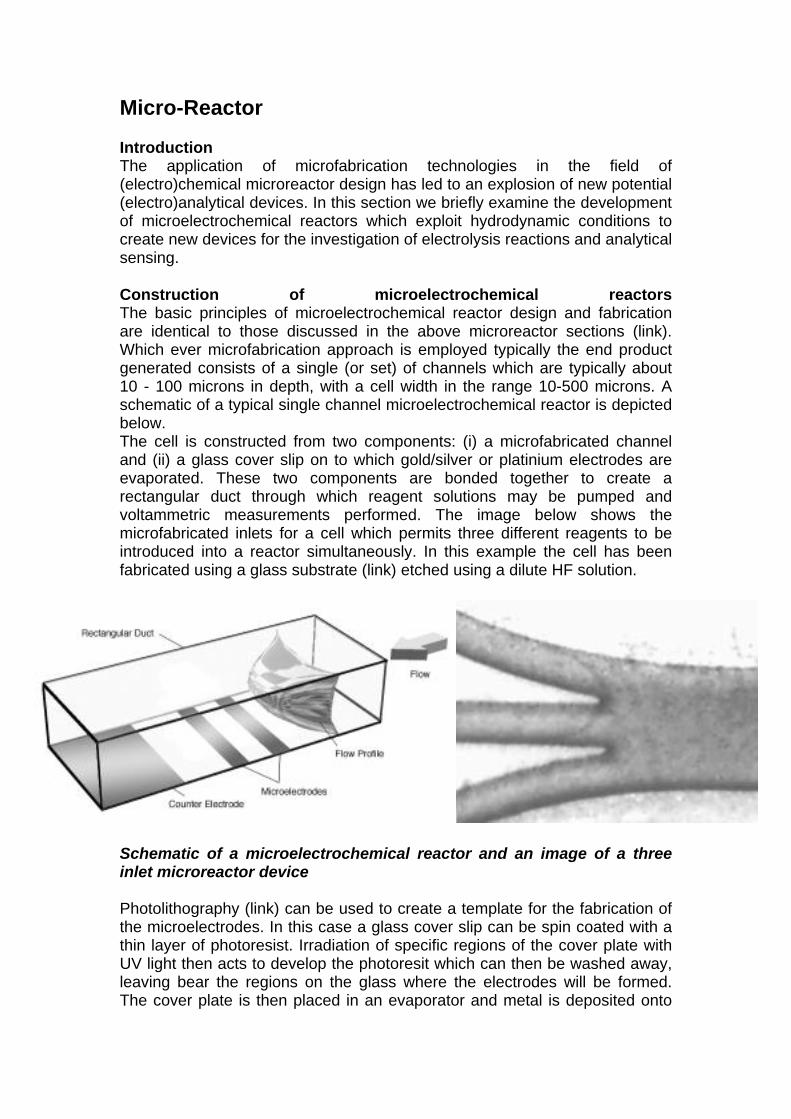
Construction of microelectrochemical reactors The basic principles of microelectrochemical reactor design and fabrication are identical to those discussed in the above microreactor sections (link). Which ever microfabrication approach is employed typically the end product generated consists of a single (or set) of channels which are typically about 10 - 100 microns in depth, with a cell width in the range 10-500 microns. A schematic of a typical single channel microelectrochemical reactor is depicted below. The cell is constructed from two components: (i) a microfabricated channel and (ii) a glass cover slip on to which gold/silver or platinium electrodes are evaporated. These two components are bonded together to create a rectangular duct through which reagent solutions may be pumped and voltammetric measurements performed. The image below shows the microfabricated inlets for a cell which permits three different reagents to be introduced into a reactor simultaneously. In this example the cell has been fabricated using a glass substrate (link) etched using a dilute HF solution.

Schematic of a microelectrochemical reactor and an image of a three inlet microreactor device Photolithography (link) can be used to create a template for the fabrication of the microelectrodes. In this case a glass cover slip can be spin coated with a thin layer of photoresist. Irradiation of specific regions of the cover plate with UV light then acts to develop the photoresit which can then be washed away, leaving bear the regions on the glass where the electrodes will be formed. The cover plate is then placed in an evaporator and metal is deposited onto

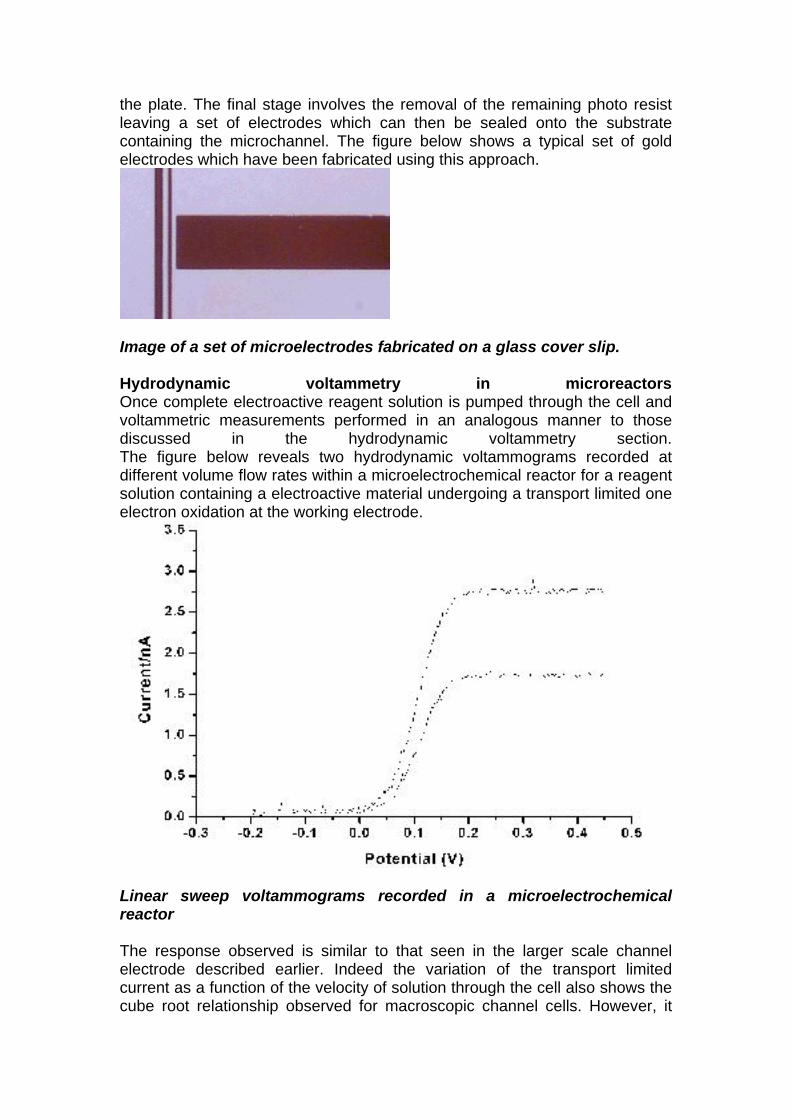
the plate. The final stage involves the removal of the remaining photo resist leaving a set of electrodes which can then be sealed onto the substrate containing the microchannel. The figure below shows a typical set of gold electrodes which have been fabricated using this approach.

Image of a set of microelectrodes fabricated on a glass cover slip. Hydrodynamic voltammetry in microreactors Once complete electroactive reagent solution is pumped through the cell and voltammetric measurements performed in an analogous manner to those discussed in the hydrodynamic voltammetry section. The figure below reveals two hydrodynamic voltammograms recorded at different volume flow rates within a microelectrochemical reactor for a reagent solution containing a electroactive material undergoing a transport limited one electron oxidation at the working electrode.

Linear sweep voltammograms recorded in a microelectrochemical reactor The response observed is similar to that seen in the larger scale channel electrode described earlier. Indeed the variation of the transport limited current as a function of the velocity of solution through the cell also shows the cube root relationship observed for macroscopic channel cells. However, it

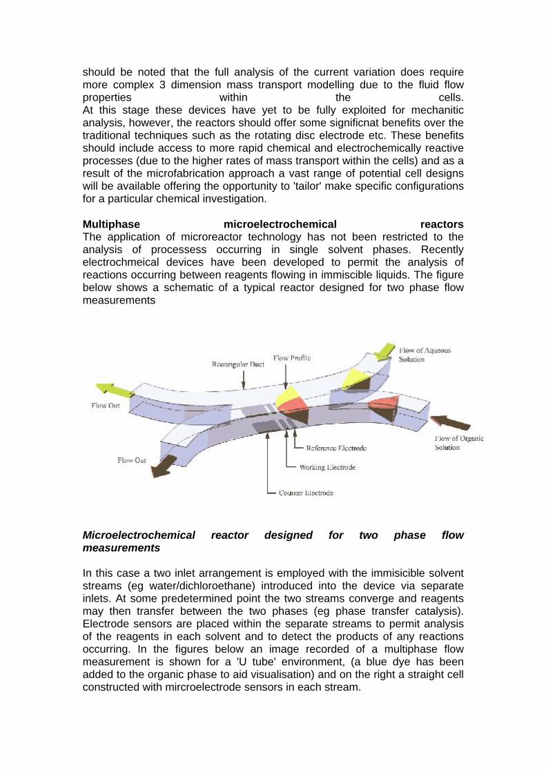
should be noted that the full analysis of the current variation does require more complex 3 dimension mass transport modelling due to the fluid flow properties within the cells. At this stage these devices have yet to be fully exploited for mechanitic analysis, however, the reactors should offer some significnat benefits over the traditional techniques such as the rotating disc electrode etc. These benefits should include access to more rapid chemical and electrochemically reactive processes (due to the higher rates of mass transport within the cells) and as a result of the microfabrication approach a vast range of potential cell designs will be available offering the opportunity to 'tailor' make specific configurations for a particular chemical investigation.

Multiphase microelectrochemical reactors The application of microreactor technology has not been restricted to the analysis of processess occurring in single solvent phases. Recently electrochmeical devices have been developed to permit the analysis of reactions occurring between reagents flowing in immiscible liquids. The figure below shows a schematic of a typical reactor designed for two phase flow measurements

Microelectrochemical reactor designed for two phase flow measurements In this case a two inlet arrangement is employed with the immisicible solvent streams (eg water/dichloroethane) introduced into the device via separate inlets. At some predetermined point the two streams converge and reagents may then transfer between the two phases (eg phase transfer catalysis). Electrode sensors are placed within the separate streams to permit analysis of the reagents in each solvent and to detect the products of any reactions occurring. In the figures below an image recorded of a multiphase flow measurement is shown for a 'U tube' environment, (a blue dye has been added to the organic phase to aid visualisation) and on the right a straight cell constructed with mircroelectrode sensors in each stream.

Images of devices used for immiscible two phase flow investigations This microreactor approach also permits more complex multiphase flow conditions to be examined. For example in the images below the approach has been extended to a three phase environment, where in this case three solvent streams containing different chemical reagents may be brought together at a predetermined point to permit chemical reaction. The figure on the left below shows the three inlet arrangement and on the right an image taken about 2.5 cms from the inlet region. It is apparent that a chemical reaction has occurred in this case an interfacial electron transfer has created the coloured product in the central stream.

Images of devices used for immiscible three phase flow investigations as a random walk model.