elastic foundation, nonlinear beam, parametric...

Journal of Mechanical Engineering and Automation 2012, 2(6): 114-134

DOI: 10.5923/j.jmea.20120206.02

Parametric Study of Nonlinear Beam Vibration Resting

on Linear Elastic Foundation

Salih N Akour

Sustainable and Renewable Energy Program, College of Engineering, University of Sharjah, PO Box 27272, Sharjah, UAE

Abstract Nonlinear beam resting on linear elastic foundation and subjected to harmonic excitation is investigated. The

beam is simply supported at both ends. Both linear and nonlinear analyses are carried out. Hamilton’s principle is utilized

in deriv ing the governing equations. Well known forced duffing oscillator equation is obtained. The equation is analyzed

numerically using Runk-Kutta technique. Three main parameters are investigated: the damping coefficient, the natural

frequency, and the coefficient of the nonlinearity. Stability reg ions for first mode analyses are unveiled. Comparison

between the linear and the nonlinear model is presented. It is shown that first mode shape the natural frequency could be

approximated as square root of the sum of squares of both natural frequency of the beam and the foundation. The stretching

potential energy is proved to be responsible for generating the cubic nonlinearity in the system.

Keywords Elastic Foundation, Nonlinear Beam, Parametric Study

1. Introduction

Beams on elastic foundations received great attention of

researches due to its wide applicat ions in engineering. The

model of the beam resting on a nonlinear support represents

a large class of mechanical systems, such as, vibrating

machines on elastic foundations, pipelines transversally

supported, disc brake pad, shafts supported on ball, roller,

or journal bearings, network of beams in the construction of

floor systems for ships, buildings, bridges, submerged

floating tunnels, railroad tracks etc. The elastic foundation

for the beam part is supplied by the resilience of the

adjoining portions of a continuous elastic structure. Hetenyi

[1] and Timoshenko[2] p resented an analytical solution for

beams on elastic supports using classical differential

equation approach, and considering several loading and

boundary conditions.

It is well known in engineering that a beam supported by

discrete elastic supports spaced at equal intervals acts

analogously to a beam on an elastic foundation and that the

appropriateness of that analogy depends on the flexural

rig idity of the beam as well as the stiffness and spacing of

the supports. Ellington investigated conditions under which

a beam on discrete elastic supports could be treated as

equivalent to a beam on elastic foundation[3].

Beams resting on elastic foundations have been studied

extensively over the years due to the wide application of

* Corresponding author:

[email protected] (Salih N Akour)

Published online at http://journal.sapub.org/jmea

Copyright © 2012 Scientific & Academic Publishing. All Rights Reserved

this system in engineering. This system according to the

literature can be d ivided at least into three categories.

The first category is “linear beam on linear elastic founda

tion”. Example of this type can be found in references[4]-[1

5]. The applications in this category include but not limited

to Euler - Bernoulli beam, Timoshenko beam, Winkler

foundation, Pasternak foundation, tensionless foundation,

single parameter or two parameter foundation, static loading,

harmonic loading and moving loading.

For example the Winkler foundation model represents the

simplest form of these types of beams. In this model the

foundation is treated essentially as an array of closely

spaced but non-interacting springs, each having a spring

stiffness that equals the foundation modulus divided by the

spacing between springs. The Pasternak foundation is

extension of Winkler foundation by introducing shear

interaction between springs. It is assumed that the top ends

of the springs are connected to an incompressible layer that

resists only transverse shear deformation. Tensionless

foundation is similar to Winkler foundation but the springs

do not carry any tension load.

The second category is “linear beam on nonlinear elastic

foundation[16]-[20]. In this category the foundation is

considered to have nonlinear stiffness. Also this type

includes different boundary and loading conditions

according to the engineering application.

The third category is nonlinear beam on linear elastic

foundation[21]-[33]. Usually the beam nonlinearity means

large deflections. Most of the studies related to this category

have analyzed the system either using boundary element

method or boundary integral equation method. Similar to

the above two categories, there is wide variety of boundary

115 Journal of Mechanical Engineering and Automation 2012, 2(6): 114-134

and loading conditions being applied to such system

according to the application.

Nonlinear beam subjected to harmonic d istributed load

resting on linear elastic foundation is investigated in this

research. The study is carried out in the view of the

linearized model of the system. Well known duffing

equation is obtained using Hamilton’s princip le. Three main

parameters are investigated: the damping coefficient, the

natural frequency, and the coefficient o f the nonlinear term.

The effect of these parameters on the system stability is

unveiled. Up to the author’s knowledge, this work is not

published in the literature.

2. Problem Statement

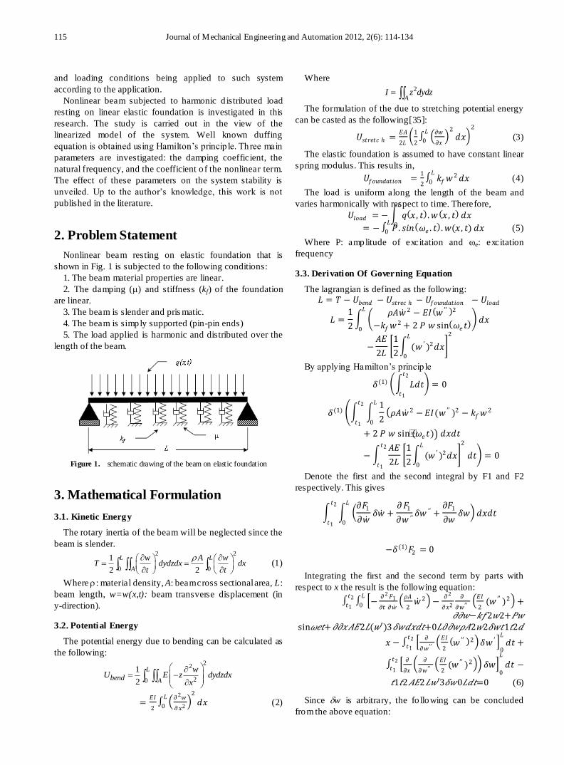
Nonlinear beam resting on elastic foundation that is

shown in Fig. 1 is subjected to the following conditions:

1. The beam material properties are linear.

2. The damping () and stiffness (kf) of the foundation

are linear.

3. The beam is slender and pris matic.

4. The beam is simply supported (pin-pin ends)

5. The load applied is harmonic and distributed over the

length of the beam.

Figure 1. schematic drawing of the beam on elastic foundation

3. Mathematical Formulation

3.1. Kinetic Energy

The rotary inertia of the beam will be neglected since the

beam is slender. 2 2

0 0

1

2 2

L L

A

w A wT dydzdx dx

t t

(1)

Where : material density, A: beam cross sectional area, L:

beam length, w=w(x,t): beam transverse displacement (in

y-direction).

3.2. Potential Energy

The potential energy due to bending can be calculated as

the following: 2

2

20

1

2

L

Abendw

U E z dydzdxx

=𝐸𝐼

2

𝜕2𝑤

𝜕𝑥2

2𝐿

0 𝑑𝑥 (2)

Where 2

AI z dydz

The formulation of the due to stretching potential energy

can be casted as the following[35]:

𝑈𝑠𝑡𝑟𝑒𝑡𝑐 ℎ =𝐸𝐴

2𝐿

1

2

𝜕𝑤

𝜕𝑥

2𝐿

0 𝑑𝑥 2

(3)

The elastic foundation is assumed to have constant linear

spring modulus. This results in,

𝑈𝑓𝑜𝑢𝑛𝑑𝑎𝑡𝑖𝑜𝑛 =1

2 𝑘𝑓𝑤

2𝐿

0 𝑑𝑥 (4)

The load is uniform along the length of the beam and

varies harmonically with respect to time. Therefore,

𝑈𝑙𝑜𝑎𝑑 = − 𝑞 𝑥 , 𝑡 . 𝑤 𝑥 , 𝑡 𝐿

0

𝑑𝑥

= − 𝑃 . 𝑠𝑖𝑛 𝜔𝑒 . 𝑡 . 𝑤(𝑥 , 𝑡)𝐿

0 𝑑𝑥 (5)

Where P: amplitude of excitation and e: excitation

frequency

3.3. Derivation Of Governing Equation

The lagrangian is defined as the following:

𝐿 = 𝑇 − 𝑈𝑏𝑒𝑛𝑑 − 𝑈𝑠𝑡𝑟𝑒𝑐 ℎ − 𝑈𝑓𝑜𝑢𝑛𝑑𝑎𝑡𝑖𝑜𝑛 − 𝑈𝑙𝑜𝑎𝑑

𝐿 =1

2

𝜌𝐴𝑤 2 − 𝐸𝐼 𝑤 ′′ 2

−𝑘𝑓𝑤2 + 2 𝑃 𝑤 sin 𝜔𝑒𝑡

𝐿

0

𝑑𝑥

−𝐴𝐸

2𝐿 1

2 (𝑤 ′ )2𝑑𝑥

𝐿

0

2

By applying Hamilton’s princip le

𝛿(1) 𝐿𝑑𝑡𝑡2

𝑡1

= 0

𝛿(1) 1

2 𝜌𝐴𝑤 2 −𝐸𝐼(𝑤 ′′ )2 − 𝑘𝑓𝑤

2𝐿

0

𝑡2

𝑡1

+ 2 𝑃 𝑤 sin(𝜔𝑒𝑡) 𝑑𝑥𝑑𝑡

− 𝐴𝐸

2𝐿 1

2 (𝑤 ′ )2𝑑𝑥

𝐿

0

2

𝑑𝑡𝑡2

𝑡1

= 0

Denote the first and the second integral by F1 and F2

respectively. This gives

𝜕𝐹1

𝜕𝑤 𝛿𝑤 +

𝜕𝐹1

𝜕𝑤 ′′𝛿𝑤 ′′ +

𝜕𝐹1

𝜕𝑤𝛿𝑤

𝐿

0

𝑡2

𝑡1

𝑑𝑥𝑑𝑡

−𝛿(1)𝐹2 = 0

Integrating the first and the second term by parts with

respect to x the result is the following equation:

−𝜕2 𝐹1

𝜕𝑡 𝜕𝑤

𝜌𝐴

2𝑤 2 −

𝜕2

𝜕𝑥2

𝜕

𝜕𝑤′′ 𝐸𝐼

2(𝑤 ′′ )2 +

𝐿

0

𝑡2

𝑡1

𝜕𝜕𝑤−𝑘𝑓2𝑤2+𝑃𝑤 sin𝜔𝑒𝑡+𝜕𝜕𝑥𝐴𝐸2𝐿(𝑤′)3𝛿𝑤𝑑𝑥𝑑𝑡+0𝐿𝜕𝜕𝑤𝜌𝐴2𝑤2𝛿𝑤𝑡1𝑡2𝑑

𝑥 − 𝜕

𝜕𝑤′′

𝐸𝐼

2 𝑤 ′′ 2 𝛿𝑤 ′

0

𝐿𝑡2

𝑡1𝑑𝑡 +

𝜕

𝜕𝑥

𝜕

𝜕𝑤′′

𝐸𝐼

2(𝑤 ′′ )2 𝛿𝑤

0

𝐿

𝑑𝑡 −𝑡2

𝑡1

𝑡1𝑡2𝐴𝐸2𝐿𝑤′3𝛿𝑤0𝐿𝑑𝑡=0 (6)

Since w is arbitrary, the fo llowing can be concluded

from the above equation:

Salih N Akour: Parametric Study of Nonlinear Beam Vibration Resting on Linear Elastic Foundation 116

The governing equation comes from setting the

expression within the brackets in Equation (6) equal to zero.

Upon carrying out the indicated differentiations, the

governing can be rewritten as

𝑤 + 𝛼𝑤 𝑖𝑣 + 𝑘𝑤 − 𝛽𝜕(𝑤 ,)3

𝜕𝑥= 𝑝sin(𝜔𝑒 𝑡) (7)

where

𝛼 =𝐸𝐼

𝜌𝐴 , 𝑘 =

𝑘𝑓

𝜌𝐴 𝑎𝑛𝑑 𝛽 =

𝐸

2𝜌𝐿

It is obvious that Equation (7) is the duffing oscillator

equation. This equation is going to be recasted into a more

familiar form in the next section. The boundary and init ial

conditions can be obtained from the remain ing terms in

Equation (6).

The boundary conditions at x=0 and x=L are

Either EIw ′′ is zero or w ′ is prescribed (8a)

Either EIw ′′ is zero or w is prescribed (8b)

Either EA

2 L(w ′ )3 is zero or w is prescribed (8c)

Boundary conditions Equation (8a) correspond to end

moments and slopes respectively. In Equation (8b), w

corresponds to end displacement, and in Equation (8c) the

first condition corresponds to pre-stretching. For the pinned

ends, the boundary conditions are:

𝑤 0 = 𝑤 𝐿 = 0

𝐸𝐼𝑤 ′′ 0 = 𝐸𝐼𝑤 ′′ 𝐿 = 0

These boundary conditions must be satisfied by the mode

shapes of the system. This fact will be used in the following

sections as the criteria fo r selecting the form of the mode

shape equation.

Finally the in itial conditions for t = t1 and t = t2 are

Either 𝜌𝐴

2(𝑤) 2 is zero or 𝑤 is prescribed

In this case, it will be assumed that the system starts from

rest i.e. the initial d isplacement and velocity is zero.

3.4. Discretization and linearization

The following expression is used for w(x, t) in order to

discretize the problem

𝑤 𝑥 , 𝑡 = 𝑤𝑛 𝑡 𝑠𝑖𝑛

𝑛𝜋𝑥

𝐿 𝑁

𝑛=1 (9)

For simplicity the limits of the above summat ion, the

subscript of w, and the time dependence of w will be

implied in the equations that follow. It is evident from

Equation (9) that the pinned ends boundary condition

Equation (8a) are satisfied since transverse displacements at

0 and L are zero, and the end slopes are free (implying zero

bending moments at the ends). Equation (9) represents

series summation of N modes each has time dependent

amplitude response, 𝑤𝑛 (𝑡) with spatial sine function.

Substituting Equation (9) into the original integral

expressions for the kinetic and potential energy of Equation

(1) through Equation (5) then applying the Lagrangian and

utilizing the orthogonality, the following equation comes

out:

𝐿 = 𝑇 − 𝑈 =𝜌𝐴

4 𝑤 2 −

𝐸𝐼𝜋4

4𝐿3 𝑛4𝑤2

−𝜋4𝐴𝐸

32𝐿3 𝑛2𝑤2 2 −

𝑘𝑓 𝐿

4 𝑤2 (10)

Lagrangian’s equation for each mode can be written as

the following: 𝑑

𝑑𝑡

𝜕𝐿

𝜕𝑤 𝑛 −

𝜕𝐿

𝜕𝑤 𝑛= 0 𝑓𝑜𝑟 𝑛 = 1,2, …… , 𝑁 (11)

Substituting Equation (10) in Equation (11) and carry out

the differentiat ion yields, 𝜌𝐴𝐿

2𝑤 𝑛 +

𝐸𝐼𝜋4𝑛4

2𝐿3𝑤𝑛 +

𝑘𝑓𝐿

2𝑤𝑛 +

𝐸𝐴𝜋4 𝑛2

8𝐿3 𝑚2 𝑤𝑚

2𝑁𝑚 =1

𝑤𝑛 = 0 (12)

A simplified form of Equation (12) results after

rearranging the coefficients and defining some new

coefficients. The concise form and the coefficient

definit ions are

w n+ ω02n4 1+

2

𝑛4 + 1

42 𝑛2 𝑚2 𝑤𝑚

2𝑁𝑚 =1 𝑤𝑛 = 0 (13)

Where

ω02 =

𝐸𝐼 𝜋4

𝜌𝐴 𝐿4,

2 =ωf2

ω02 ,ωf

2 =𝑘𝑓

𝜌𝐴 𝑎𝑛𝑑 =

𝐼

𝐴

Writing Equation (13) for a single mode and inserting the

linear damping term g ives,

w n+ 2μ𝑤 𝑛 + ω02n4 1+

2

𝑛4 𝑤𝑛 +

ω02n2

42 𝑤𝑛3 = 0 (14)

Where µ is the damping coefficient

This makes it clear that the above equation represent

unforced damped duffing oscillator. Recasting Equation (14)

into the following:

𝑤 + 2μ𝑤 + 𝜔2𝑤 + 𝛼 𝑤3 = 0 (15)

Where

𝜔2 = ω02n4 1+

2

𝑛4 𝑎𝑛𝑑 𝛼 =

ω02n2

42

In order to linearize the system for the first mode (n=1)

the system is converted into first order ordinary differential

equations by the following substitution

𝑋 = 𝑤 → 𝑋 = 𝑤 𝑌 = 𝑤 → 𝑌 = 𝑤

Applying this to Equation (15)

𝑋 = 𝑌 , 𝑌 = − 2μ𝑌 − 𝜔2𝑋 − 𝛼 𝑋3

𝑌 = 0 , − 2μ𝑌 − 𝜔2𝑋 − 𝛼 𝑋3 = 0

From the above equations it is obvious that (0, 0) is the

only critical point for the system. So the equivalent linear

system is obtained by expanding the above equation using

Taylor series about (0, 0), so the remain ing linear terms are

𝑋 = 𝑌 , 𝑌 = − 2μ𝑌 − 𝜔2𝑋

The corresponding Jacobi matrix is

𝐽 = 0 1

−𝜔2 − 2μ

So the Eigenvalues of J are

1 ,2 = −𝜇 ± 𝜇2 − 𝜔2

2 − 𝑝 + 𝑞 = 0,

𝑤ℎ𝑒𝑟𝑒 𝑝 = −2µ 𝑎𝑛𝑑 𝑞 = 𝜔2

Introducing as

= µ2 − 𝜔2

the following can be said about (0, 0):

a. For 𝜇 > 0 :


Stable attractive node for ≥ 0

Stable spiral attractive node < 0

b. Stable center if 𝜇 = 0 ;

c. Unstable if 𝜇 < 0.

The general solution of the linearized unforced system is

𝑋 𝑡 = 𝐶1𝑒1 𝑡 + 𝐶2𝑒

2 𝑡

𝑋 𝑡 = 𝑒−µ𝑡(𝐶1𝑒− 𝑡 + 𝐶2𝑒

𝑡)

Applying the init ial conditions (0) = 𝑥0 , 𝑋 (0) = 𝑥 0 the

constants of integration are going to be as the following:

𝐶1 = − 𝜇 𝑥0 − 𝑥 0

2 ,

𝐶2 = + 𝜇 𝑥0 + 𝑥 0

2

3.5. Simulation of the nonlinear system

𝑤 + 2μ𝑤 + 𝜔2𝑤 + 𝛼 𝑤3 = 𝑃 sin(𝜔𝑒 𝑡) (16)

where

𝜔2 = ω02 n4 1+

2

𝑛4 ,

2 =ωf

2

ω02 , 𝛼 =

ω02 n2

42

, ω02 =

𝐸𝐼𝜋4

𝜌𝐴𝐿4 , 𝑛 = 1, ωf

2 =𝑘𝑓

𝜌𝐴,

𝑎𝑛𝑑

= 𝐼

𝐴

It is obvious that the strength of the nonlinearity is

inversely proportional to the square of the radius of gyration

of the beam. This indicates that the nonlinearity remains

weak as long as the beam is relat ively slender as assumed in

this study. Finally, the frequency equation can be simplified

to 𝜔2 = ω02 + ωf

2.

The apparent natural frequency of the system is the

square root of the sum of the squares of the natural

frequencies of the beam and the elastic foundation.

The nonlinear second order ordinary d ifferential equation

is converted into a system of first order o rdinary d ifferential

equations. This is suitable fo r numerical study using

Runge-Kutta Techniques.

𝑍 = 𝑤 𝑍 = 𝑤 = 𝑃 sin(𝜔𝑒 𝑡) − 2μ𝑤 − 𝜔2𝑤 − 𝛼 𝑤3 (17)

4. Results and Discussion

The results for simply supported beam on elastic

foundation are presented in Figures 2 through 6, Table 1

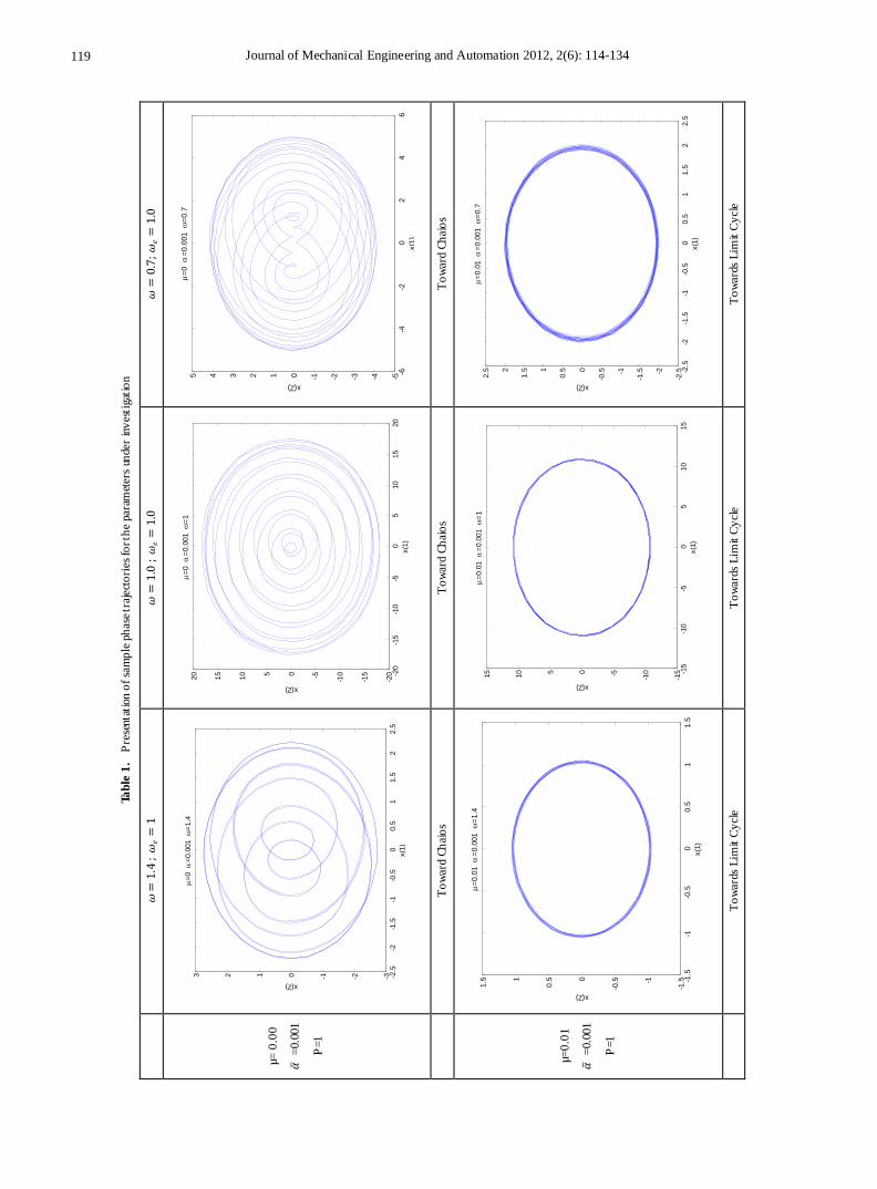
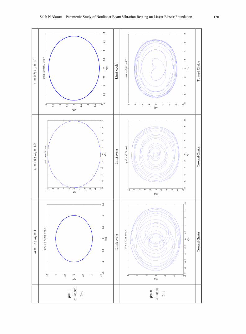
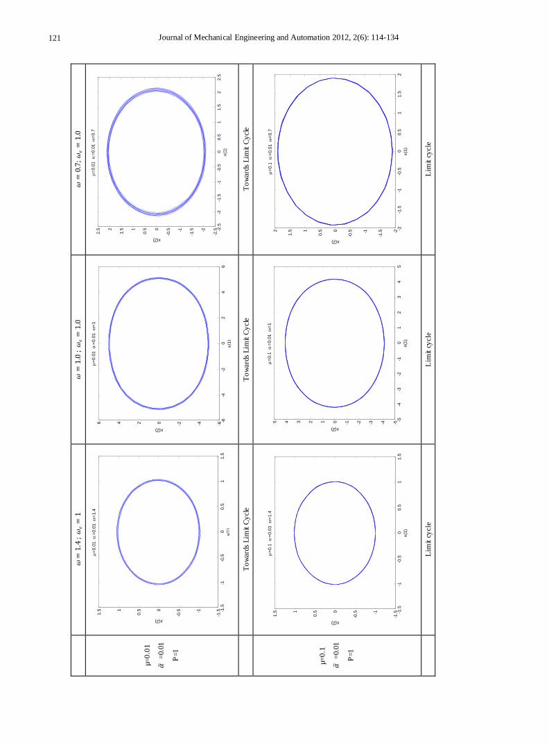
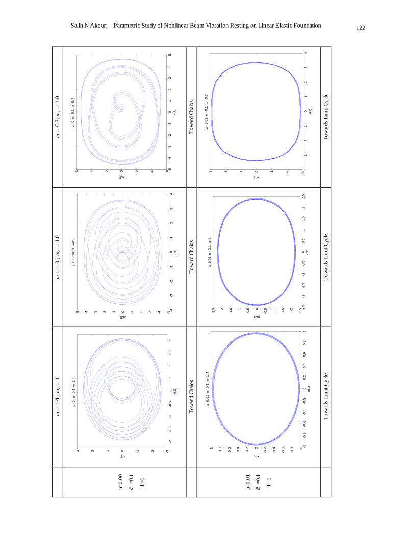
and Table 2. Figures 2 through 6 present the results of the

linearized model whereas Table 1, 2 and 3 represent the

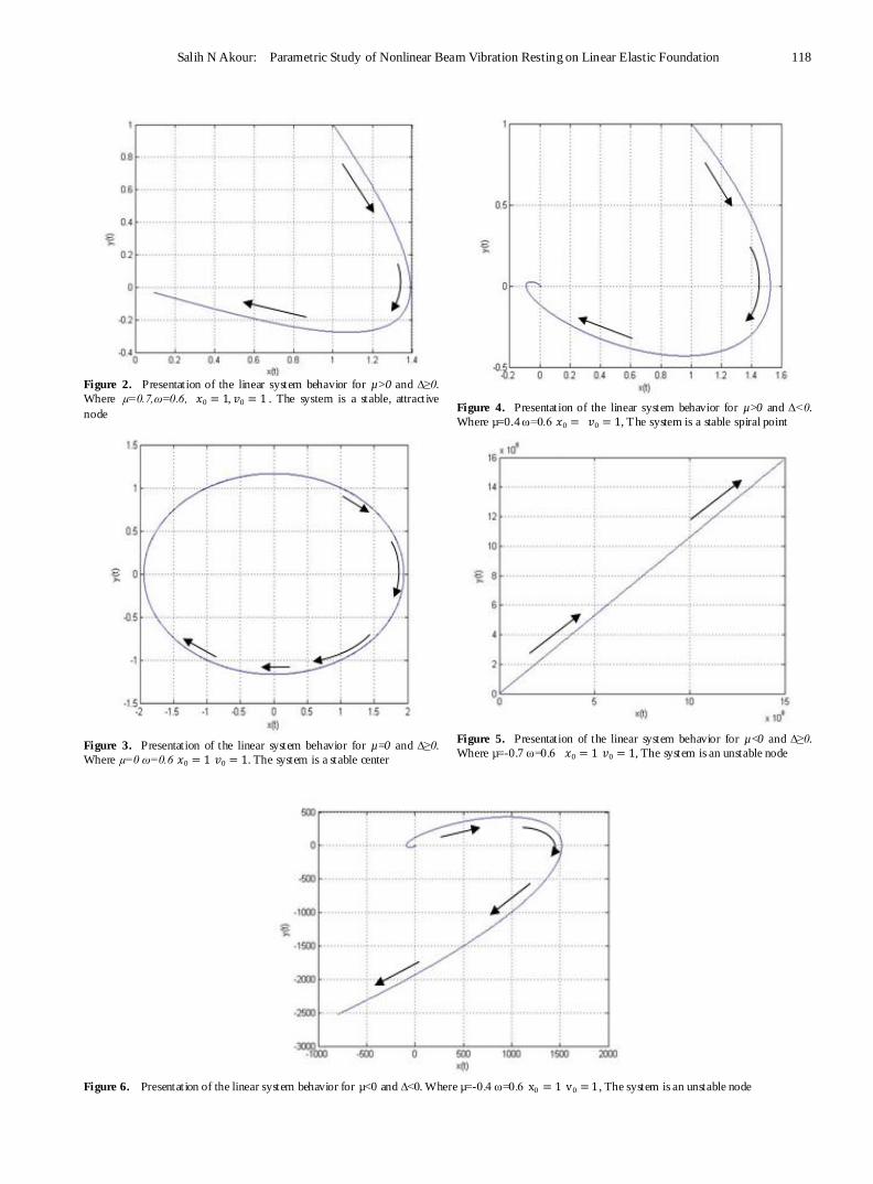
results of the nonlinear model. Figure 2 present the linear

system behavior for µ>0 and ∆≥0. It is obvious that the

system is stable attractive node. Table 1 represents sample

phase diagrams of the studied ranges. Figure 3 shows stable

centre for the linear system of µ=0 and ∆≥0. Figure 4

presents stable spiral for the linear system behavior of µ>0

and ∆<0. In Figures 2, 3 and 4 the system is stable however

in Figures 5 and 6 it is not stable. The behavior in both

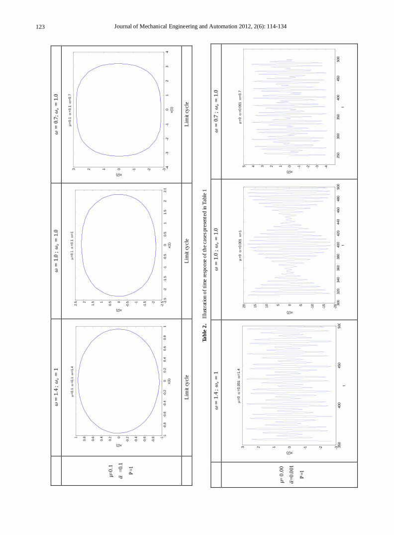
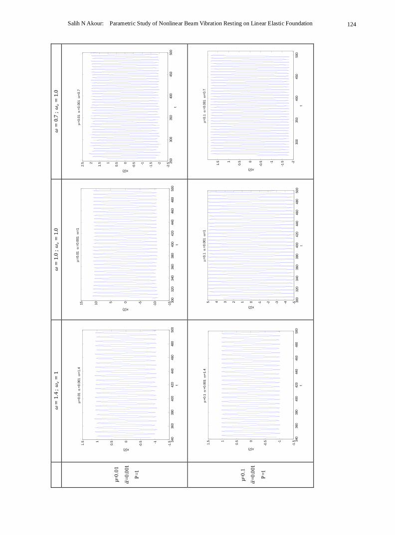
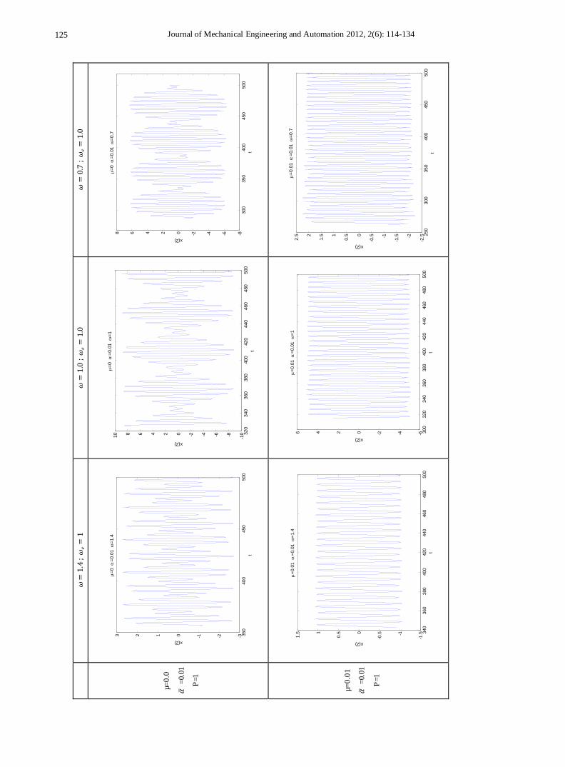
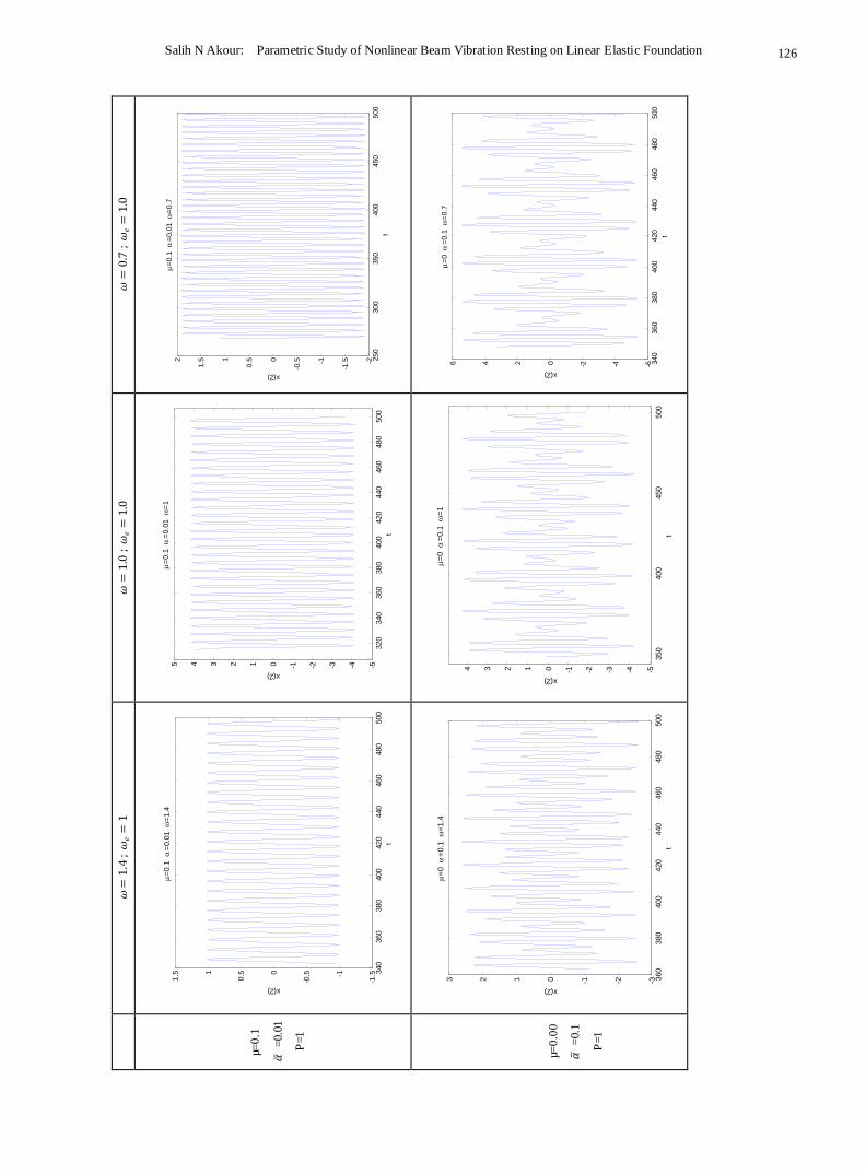
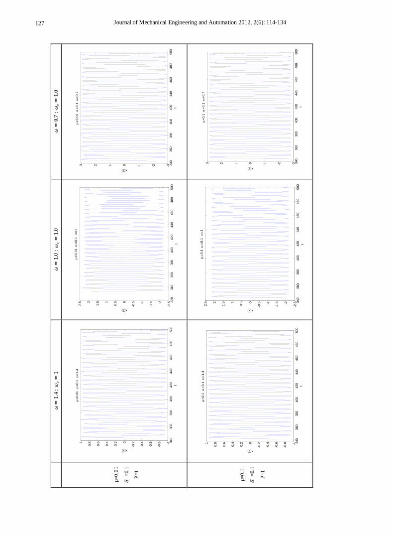
Figures 5 and 6 is unstable node. Table 2 shows the time

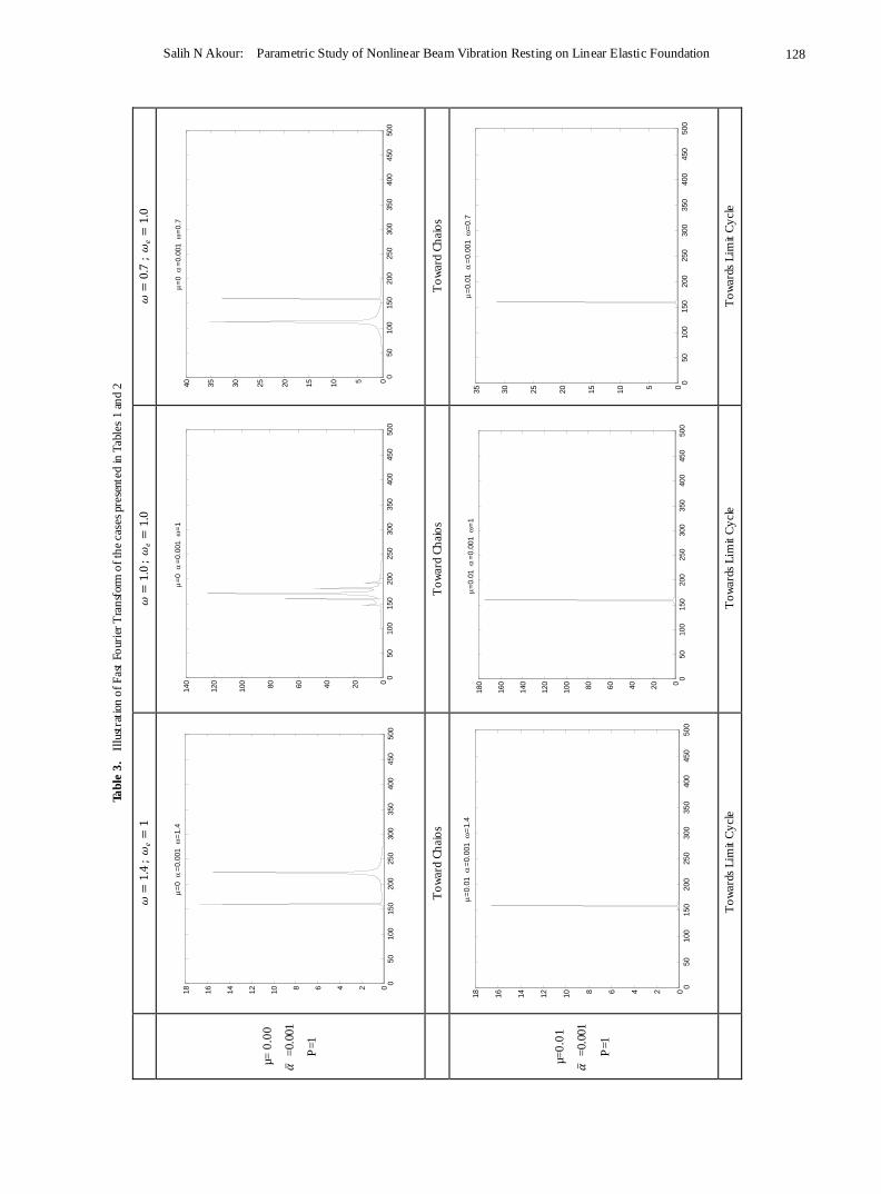
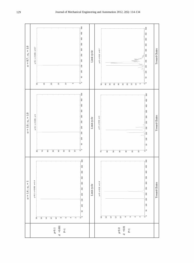
response for those cases that are presented in Table 1,

whereas the corresponding frequency spectra (Fast Fourier

Transform-FFT) for those cases presented in both Tables 1

and 2. The phase portraits and the time response are

collected after long period of t ime to be sure that the system

has passed the transient range. The duffing Equation (16) is

converted into system of first order ord inary d ifferential

equation as shown in Equation (17) and solved using

MATLAB package by utilizing the Runga-Kutta ODE

(Ordinary Differential Equation) solver. The equation

which represents the system under investigation is of cubic

nonlinearity with harmonic excitation.

The sample results present the effect of damping when

the system has weak, medium and strong nonlinearity for

excitation frequencies below, at and above resonance. The

whole study is considering weak nonlinearity that does not

exceed α =0.1 and those levels of weak, medium and

strong within that range. Only the first mode is considered

in this study. The parameters range covered in this

investigation are for =0.0 through 0.1, α = 0.001 through

0.1 and natural frequency = 0.7 through 1.4. It can be seen

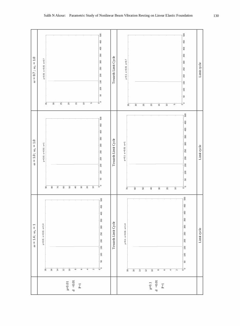
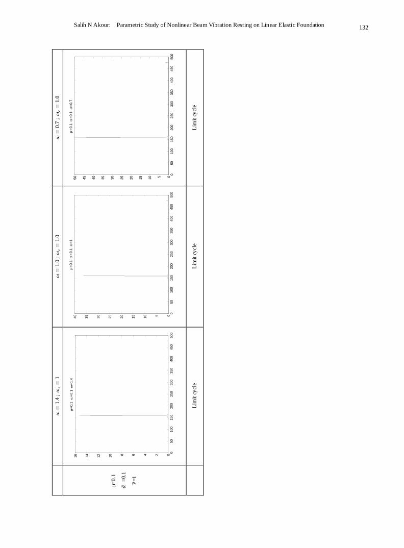
from Table 1 that when there is no damping the system is

tending toward chaos however when little damping is

applied the system is tending towards limit cycle.

It is obvious that the damping and the nonlinearity are the

most effective parameters in controlling the chaotic

behavior of the system. As long as the radius of gyration for

the beam under consideration is large i.e., the beam is more

towards slender, the nonlinearity is going to be weak. This

means that the contribution of the stretching energy to the

behavior of the system is going to be low. The damping

system dissipates the oscillat ing energy and provides a

control over the system behavior. For the linear system, as

long as damping coefficient is positive, the transient

response is going to decrease exponentially and the forcing

excitation response is bounded even at resonance. For

undamped linear system the forcing excitation response is

not bounded and the response is increasing with time. For

the nonlinear system, the response is tending toward chaos

as it can be seen in Tab le 1 for =0.0. However when the

damping increases the system is transferring from chaos to

limit cycle. It is obvious in Table 3 that all cases of =0.0

have Double period, Trip le period, or, Chaotic response.

The response of those double period cases shows amplitude

modulation whereas those cases where their frequencies are

very close show beating phenomenon. For the resonance

case of no damping i.e., the excitation frequency equals the

natural frequency, the linear system has increasing

amplitude response whereas the nonlinear system is tending

towards chaos with bounded amplitude. It is obvious that

the nonlinear cases (within the range of investigation) are

tending towards chaos as long as there is no damping in the

system.


Figure 2. Presentation of the linear system behavior for µ>0 and ∆≥0.

Where µ=0.7,ω=0.6, 𝑥0 = 1, 𝑣0 = 1 . The system is a stable, attractive

node

Figure 3. Presentation of the linear system behavior for µ=0 and ∆≥0.

Where µ=0 ω=0.6 𝑥0 = 1 𝑣0 = 1. The system is a stable center

Figure 4. Presentation of the linear system behavior for µ>0 and ∆<0.

Where µ=0.4 ω=0.6 𝑥0 = 𝑣0 = 1, The system is a stable spiral point

Figure 5. Presentation of the linear system behavior for µ<0 and ∆≥0.

Where µ=-0.7 ω=0.6 𝑥0 = 1 𝑣0 = 1, The system is an unstable node

Figure 6. Presentation of the linear system behavior for µ<0 and ∆<0. Where µ=-0.4 ω=0.6 x0 = 1 v0 = 1 , The system is an unstable node

1

Journ

al o

f M

echan

ical

En

gineer

ing

and

Auto

mat

ion

2012, 2(6

): 1

14

-134

Ta

ble

1.

Pre

senta

tion

of

sam

ple

ph

ase

traj

ecto

ries

fo

r th

e par

amet

ers

under

inv

esti

gat

ion

𝜔

=1

.4 ;

𝜔𝑒

=1

𝜔

=1

.0 ;

𝜔𝑒

=1

.0

𝜔=

0.7

; 𝜔

𝑒=

1.0

µ=

0.0

0

𝛼

=0.0

01

P=1

T

ow

ard C

hai

os

To

war

d C

hai

os

To

war

d C

hai

os

µ=

0.0

1

𝛼

=0.0

01

P=1

T

ow

ards

Lim

it C

ycl

e T

ow

ards

Lim

it C

ycl

e T

ow

ards

Lim

it C

ycl

e

-2.5

-2-1

.5-1

-0.5

00.5

11.5

22.5

-3-2-10123

=0

=0.0

01

=1.4

x(1

)

x(2)

-20

-15

-10

-50

510

15

20

-20

-15

-10-505

10

15

20

=

0

=0.0

01

=1

x(1

)

x(2)

-6-4

-20

24

6-5-4-3-2-1012345

=

0

=0.0

01

=0.7

x(1

)

x(2)

-1.5

-1-0

.50

0.5

11.5

-1.5-1

-0.50

0.51

1.5

=

0.0

1

=0.0

01

=1.4

x(1

)

x(2)

-15

-10

-50

510

15

-15

-10-505

10

15

=

0.0

1

=0.0

01

=1

x(1

)

x(2)

-2.5

-2-1

.5-1

-0.5

00.5

11.5

22.5

-2.5-2

-1.5-1

-0.50

0.51

1.52

2.5

=

0.0

1

=0.0

01

=0.7

x(1

)

x(2)

Journal of Mechanical Engineering and Automation 2012, 2(6): 114-134 119

Sal

ih N

Akour:

Par

amet

ric

Stu

dy

of

Nonlinea

r B

eam

Vib

rati

on R

esti

ng

on L

inea

r E

last

ic F

oundat

ion

2

𝜔

=1

.4 ;

𝜔𝑒

=1

𝜔

=1

.0 ;

𝜔𝑒

=1

.0

𝜔=

0.7

; 𝜔

𝑒=

1.0

µ=

0.1

𝛼

=0.0

01

P=1

L

imit c

ycl

e L

imit c

ycl

e L

imit c

ycl

e

µ=

0.0

𝛼

=0.0

1

P=1

T

ow

ard C

hai

os

To

war

d C

hai

os

To

war

d C

hai

os

-1.5

-1-0

.50

0.5

11.5

-1.5-1

-0.50

0.51

1.5

=

0.1

=0.0

01

=1.4

x(1

)

x(2)

-5-4

-3-2

-10

12

34

5-5-4-3-2-1012345

=

0.1

=0.0

01

=1

x(1

)

x(2)

-2-1

.5-1

-0.5

00.5

11.5

2-2

-1.5-1

-0.50

0.51

1.52

=

0.1

=0.0

01

=0.7

x(1

)

x(2)

-2.5

-2-1

.5-1

-0.5

00.5

11.5

22.5

-3-2-10123

=0

=0.0

1

=1.4

x(1

)

x(2)

-10

-8-6

-4-2

02

46

810

-10-8-6-4-202468

10

=

0

=0.0

1

=1

x(1

)

x(2)

-8-6

-4-2

02

46

8-8-6-4-202468

=

0

=0.0

1

=0.7

x(1

)

x(2)


3

Journ

al o

f M

echan

ical

En

gineer

ing

and

Auto

mat

ion

2012, 2(6

): 1

14

-134

𝜔

=1

.4 ;

𝜔𝑒

=1

𝜔

=1

.0 ;

𝜔𝑒

=1

.0

𝜔=

0.7

; 𝜔

𝑒=

1.0

µ=

0.0

1

𝛼

=0.0

1

P=1

T

ow

ards

Lim

it C

ycl

e T

ow

ards

Lim

it C

ycl

e T

ow

ards

Lim

it C

ycl

e

µ=

0.1

𝛼

=0.0

1

P=1

L

imit c

ycl

e L

imit c

ycl

e L

imit c

ycl

e

-1.5

-1-0

.50

0.5

11.5

-1.5-1

-0.50

0.51

1.5

=

0.0

1

=0.0

1

=1.4

x(1

)

x(2)

-6-4

-20

24

6-6-4-20246

=

0.0

1

=0.0

1

=1

x(1

)

x(2)

-2.5

-2-1

.5-1

-0.5

00.5

11.5

22.5

-2.5-2

-1.5-1

-0.50

0.51

1.52

2.5

=

0.0

1

=0.0

1

=0.7

x(1

)

x(2)

-1.5

-1-0

.50

0.5

11.5

-1.5-1

-0.50

0.51

1.5

=

0.1

=0.0

1

=1.4

x(1

)

x(2)

-5-4

-3-2

-10

12

34

5-5-4-3-2-1012345

=

0.1

=0.0

1

=1

x(1

)

x(2)

-2-1

.5-1

-0.5

00.5

11.5

2-2

-1.5-1

-0.50

0.51

1.52

=

0.1

=0.0

1

=0.7

x(1

)

x(2)


Sal

ih N

Akour:

Par

amet

ric

Stu

dy

of

Nonlinea

r B

eam

Vib

rati

on R

esti

ng

on L

inea

r E

last

ic F

oundat

ion

4

𝜔

=1

.4 ;

𝜔𝑒

=1

𝜔

=1

.0 ;

𝜔𝑒

=1

.0

𝜔=

0.7

; 𝜔

𝑒=

1.0

µ=

0.0

0

𝛼

=0.1

P=1

T

ow

ard C

hai

os

To

war

d C

hai

os

To

war

d C

hai

os

µ=

0.0

1

𝛼

=0.1

P=1

T

ow

ards

Lim

it C

ycl

e T

ow

ards

Lim

it C

ycl

e T

ow

ards

Lim

it C

ycl

e

-2-1

.5-1

-0.5

00.5

11.5

2-3-2-10123

=

0

=0.1

=1.4

x(1

)

x(2)

-4-3

-2-1

01

23

4-5-4-3-2-1012345

=

0

=0.1

=1

x(1

)

x(2)

-5-4

-3-2

-10

12

34

5-6-4-20246

=

0

=0.1

=0.7

x(1

)

x(2)

-1-0

.8-0

.6-0

.4-0

.20

0.2

0.4

0.6

0.8

1-1

-0.8

-0.6

-0.4

-0.20

0.2

0.4

0.6

0.81

=

0.0

1

=0.1

=1.4

x(1

)

x(2)

-2.5

-2-1

.5-1

-0.5

00.5

11.5

22.5

-2.5-2

-1.5-1

-0.50

0.51

1.52

2.5

=

0.0

1

=0.1

=1

x(1

)

x(2)

-4-3

-2-1

01

23

4-3-2-10123

=

0.0

1

=0.1

=0.7

x(1

)

x(2)


5

Journ

al o

f M

echan

ical

En

gineer

ing

and

Auto

mat

ion

2012, 2(6

): 1

14

-134

𝜔

=1

.4 ;

𝜔𝑒

=1

𝜔

=1

.0 ;

𝜔𝑒

=1

.0

𝜔=

0.7

; 𝜔

𝑒=

1.0

µ=

0.1

𝛼

=0.1

P=1

L

imit c

ycl

e L

imit c

ycl

e L

imit c

ycl

e

Ta

ble

2.

Il

lust

rati

on

of

tim

e re

spo

nse

of

the

case

s pre

sente

d in

Tab

le 1

𝜔

=1

.4 ;

𝜔𝑒

=1

𝜔

=1

.0 ;

𝜔𝑒

=1

.0

𝜔=

0.7

; 𝜔

𝑒=

1.0

µ=

0.0

0

𝛼 =

0.0

01

P=1

-1-0

.8-0

.6-0

.4-0

.20

0.2

0.4

0.6

0.8

1-1

-0.8

-0.6

-0.4

-0.20

0.2

0.4

0.6

0.81

=

0.1

=0.1

=1.4

x(1

)

x(2)

-2.5

-2-1

.5-1

-0.5

00.5

11.5

22.5

-2.5-2

-1.5-1

-0.50

0.51

1.52

2.5

=

0.1

=0.1

=1

x(1

)

x(2)

-4-3

-2-1

01

23

4-3-2-10123

=

0.1

=0.1

=0.7

x(1

)

x(2)

350

400

450

500

-3-2-10123

t

x(2)

=

0

=0.0

01

=1.4

300

320

340

360

380

400

420

440

460

480

500

-20

-15

-10-505

10

15

20

t

x(2)

=

0

=0.0

01

=1

250

300

350

400

450

500

-4-3-2-1012345

t

x(2)

=

0

=0.0

01

=0.7


Sal

ih N

Akour:

Par

amet

ric

Stu

dy

of

Nonlinea

r B

eam

Vib

rati

on R

esti

ng

on L

inea

r E

last

ic F

oundat

ion

6

𝜔

=1

.4 ;

𝜔𝑒

=1

𝜔

=1

.0 ;

𝜔𝑒

=1

.0

𝜔=

0.7

; 𝜔

𝑒=

1.0

µ=

0.0

1

𝛼 =

0.0

01

P=1

µ=

0.1

𝛼 =

0.0

01

P=1

340

360

380

400

420

440

460

480

500

-1.5-1

-0.50

0.51

1.5

t

x(2)

=

0.0

1

=0.0

01

=1.4

300

320

340

360

380

400

420

440

460

480

500

-15

-10-505

10

15

t

x(2)

=

0.0

1

=0.0

01

=1

250

300

350

400

450

500

-2.5-2

-1.5-1

-0.50

0.51

1.52

2.5

t

x(2)

=

0.0

1

=0.0

01

=0.7

340

360

380

400

420

440

460

480

500

-1.5-1

-0.50

0.51

1.5

t

x(2)

=

0.1

=0.0

01

=1.4

300

320

340

360

380

400

420

440

460

480

500

-5-4-3-2-1012345

t

x(2)

=

0.1

=0.0

01

=1

300

350

400

450

500

-2

-1.5-1

-0.50

0.51

1.5

t

x(2)

=

0.1

=0.0

01

=0.7


7

Journ

al o

f M

echan

ical

En

gineer

ing

and

Auto

mat

ion

2012, 2(6

): 1

14

-134

𝜔

=1

.4 ;

𝜔𝑒

=1

𝜔

=1

.0 ;

𝜔𝑒

=1

.0

𝜔=

0.7

; 𝜔

𝑒=

1.0

µ=

0.0

𝛼

=0.0

1

P=1

µ=

0.0

1

𝛼

=0.0

1

P=1

350

400

450

500

-3-2-10123

t

x(2)

=

0

=0.0

1

=1.4

320

340

360

380

400

420

440

460

480

500

-10-8-6-4-202468

10

t

x(2)

=

0

=0.0

1

=1

300

350

400

450

500

-8-6-4-202468

t

x(2)

=

0

=0.0

1

=0.7

340

360

380

400

420

440

460

480

500

-1.5-1

-0.50

0.51

1.5

t

x(2)

=

0.0

1

=0.0

1

=1.4

300

320

340

360

380

400

420

440

460

480

500

-6-4-20246

t

x(2)

=

0.0

1

=0.0

1

=1

250

300

350

400

450

500

-2.5-2

-1.5-1

-0.50

0.51

1.52

2.5

t

x(2)

=

0.0

1

=0.0

1

=0.7


Sal

ih N

Akour:

Par

amet

ric

Stu

dy

of

Nonlinea

r B

eam

Vib

rati

on R

esti

ng

on L

inea

r E

last

ic F

oundat

ion

8

𝜔

=1

.4 ;

𝜔𝑒

=1

𝜔

=1

.0 ;

𝜔𝑒

=1

.0

𝜔=

0.7

; 𝜔

𝑒=

1.0

µ=

0.1

𝛼

=0.0

1

P=1

µ=

0.0

0

𝛼

=0.1

P=1

340

360

380

400

420

440

460

480

500

-1.5-1

-0.50

0.51

1.5

t

x(2)

=

0.1

=0.0

1

=1.4

320

340

360

380

400

420

440

460

480

500

-5-4-3-2-1012345

t

x(2)

=

0.1

=0.0

1

=1

250

300

350

400

450

500

-2

-1.5-1

-0.50

0.51

1.52

t

x(2)

=

0.1

=0.0

1

=0.7

360

380

400

420

440

460

480

500

-3-2-10123

t

x(2)

=

0

=0.1

=1.4

350

400

450

500

-5-4-3-2-101234

t

x(2)

=

0

=0.1

=1

340

360

380

400

420

440

460

480

500

-6-4-20246

t

x(2)

=

0

=0.1

=0.7


9

Journ

al o

f M

echan

ical

En

gineer

ing

and

Auto

mat

ion

2012, 2(6

): 1

14

-134

𝜔

=1

.4 ;

𝜔𝑒

=1

𝜔

=1

.0 ;

𝜔𝑒

=1

.0

𝜔=

0.7

; 𝜔

𝑒=

1.0

µ=

0.0

1

𝛼

=0.1

P=1

µ=

0.1

𝛼

=0.1

P=1

340

360

380

400

420

440

460

480

500

-1

-0.8

-0.6

-0.4

-0.20

0.2

0.4

0.6

0.81

t

x(2)

=

0.0

1

=0.1

=1.4

320

340

360

380

400

420

440

460

480

500

-2.5-2

-1.5-1

-0.50

0.51

1.52

2.5

t

x(2)

=

0.0

1

=0.1

=1

340

360

380

400

420

440

460

480

500

-3-2-10123

t

x(2)

=

0.0

1

=0.1

=0.7

340

360

380

400

420

440

460

480

500

-1

-0.8

-0.6

-0.4

-0.20

0.2

0.4

0.6

0.81

t

x(2)

=

0.1

=0.1

=1.4

340

360

380

400

420

440

460

480

500

-2.5-2

-1.5-1

-0.50

0.51

1.52

2.5

t

x(2)

=

0.1

=0.1

=1

340

360

380

400

420

440

460

480

500

-3-2-10123

t

x(2)

=

0.1

=0.1

=0.7


Sal

ih N

Akour:

Par

amet

ric

Stu

dy

of

Nonlinea

r B

eam

Vib

rati

on R

esti

ng

on L

inea

r E

last

ic F

oundat

ion

10

Ta

ble

3.

Il

lust

rati

on

of

Fas

t Fo

uri

er T

ran

sform

of

the

case

s pre

sente

d in

Tab

les

1 a

nd 2

𝜔

=1

.4 ;

𝜔𝑒

=1

𝜔

=1

.0 ;

𝜔𝑒

=1

.0

𝜔=

0.7

; 𝜔

𝑒=

1.0

µ=

0.0

0

𝛼

=0.0

01

P=1

T

ow

ard C

hai

os

To

war

d C

hai

os

To

war

d C

hai

os

µ=

0.0

1

𝛼

=0.0

01

P=1

T

ow

ards

Lim

it C

ycl

e T

ow

ards

Lim

it C

ycl

e T

ow

ards

Lim

it C

ycl

e

050

100

150

200

250

300

350

400

450

500

02468

10

12

14

16

18

=

0

=0.0

01

=1.4

050

100

150

200

250

300

350

400

450

500

0

20

40

60

80

100

120

140

=

0

=0.0

01

=1

050

100

150

200

250

300

350

400

450

500

05

10

15

20

25

30

35

40

=

0

=0.0

01

=0.7

050

100

150

200

250

300

350

400

450

500

02468

10

12

14

16

18

=

0.0

1

=0.0

01

=1.4

050

100

150

200

250

300

350

400

450

500

0

20

40

60

80

100

120

140

160

180

=

0.0

1

=0.0

01

=1

050

100

150

200

250

300

350

400

450

500

05

10

15

20

25

30

35

=

0.0

1

=0.0

01

=0.7


11

Journ

al o

f M

echan

ical

En

gineer

ing

and

Auto

mat

ion

2012, 2(6

): 1

14

-134

𝜔

=1

.4 ;

𝜔𝑒

=1

𝜔

=1

.0 ;

𝜔𝑒

=1

.0

𝜔=

0.7

; 𝜔

𝑒=

1.0

µ=

0.1

𝛼

=0.0

01

P=1

L

imit c

ycl

e L

imit c

ycl

e L

imit c

ycl

e

µ=

0.0

𝛼

=0.0

1

P=1

T

ow

ard C

hai

os

To

war

d C

hai

os

To

war

d C

hai

os

050

100

150

200

250

300

350

400

450

500

02468

10

12

14

16

18

=

0.1

=0.0

01

=1.4

050

100

150

200

250

300

350

400

450

500

0

10

20

30

40

50

60

70

80

=

0.1

=0.0

01

=1

050

100

150

200

250

300

350

400

450

500

05

10

15

20

25

30

=

0.1

=0.0

01

=0.7

050

100

150

200

250

300

350

400

450

500

02468

10

12

14

16

18

=

0

=0.0

1

=1.4

050

100

150

200

250

300

350

400

450

500

0

10

20

30

40

50

60

70

=

0

=0.0

1

=1

050

100

150

200

250

300

350

400

450

500

05

10

15

20

25

30

35

40

45

50

=

0

=0.0

1

=0.7


Sal

ih N

Akour:

Par

amet

ric

Stu

dy

of

Nonlinea

r B

eam

Vib

rati

on R

esti

ng

on L

inea

r E

last

ic F

oundat

ion

12

𝜔

=1

.4 ;

𝜔𝑒

=1

𝜔

=1

.0 ;

𝜔𝑒

=1

.0

𝜔=

0.7

; 𝜔

𝑒=

1.0

µ=

0.0

1

𝛼

=0.0

1

P=1

T

ow

ards

Lim

it C

ycl

e T

ow

ards

Lim

it C

ycl

e T

ow

ards

Lim

it C

ycl

e

µ=

0.1

𝛼

=0.0

1

P=1

L

imit c

ycl

e L

imit c

ycl

e L

imit c

ycl

e

050

100

150

200

250

300

350

400

450

500

02468

10

12

14

16

18

=

0.0

1

=0.0

1

=1.4

050

100

150

200

250

300

350

400

450

500

0

10

20

30

40

50

60

70

80

90

=

0.0

1

=0.0

1

=1

050

100

150

200

250

300

350

400

450

500

05

10

15

20

25

30

35

=

0.0

1

=0.0

1

=0.7

050

100

150

200

250

300

350

400

450

500

02468

10

12

14

16

18

=

0.1

=0.0

1

=1.4

050

100

150

200

250

300

350

400

450

500

0

10

20

30

40

50

60

70

=

0.1

=0.0

1

=1

050

100

150

200

250

300

350

400

450

500

05

10

15

20

25

30

35

=

0.1

=0.0

1

=0.7


13

Journ

al o

f M

echan

ical

En

gineer

ing

and

Auto

mat

ion

2012, 2(6

): 1

14

-134

𝜔

=1

.4 ;

𝜔𝑒

=1

𝜔

=1

.0 ;

𝜔𝑒

=1

.0

𝜔=

0.7

; 𝜔

𝑒=

1.0

µ=

0.0

0

𝛼

=0.1

P=1

T

ow

ard C

hai

os

To

war

d C

hai

os

To

war

d C

hai

os

µ=

0.0

1

𝛼

=0.1

P=1

T

ow

ards

Lim

it C

ycl

e T

ow

ards

Lim

it C

ycl

e T

ow

ards

Lim

it C

ycl

e

050

100

150

200

250

300

350

400

450

500

02468

10

12

14

16

18

20

=

0

=0.1

=1.4

050

100

150

200

250

300

350

400

450

500

05

10

15

20

25

30

=

0

=0.1

=1

050

100

150

200

250

300

350

400

450

500

05

10

15

20

25

30

=

0

=0.1

=0.7

050

100

150

200

250

300

350

400

450

500

02468

10

12

14

16

=

0.0

1

=0.1

=1.4

050

100

150

200

250

300

350

400

450

500

05

10

15

20

25

30

35

40

=

0.0

1

=0.1

=1

050

100

150

200

250

300

350

400

450

500

0

10

20

30

40

50

60

=

0.0

1

=0.1

=0.7


Sal

ih N

Akour:

Par

amet

ric

Stu

dy

of

Nonlinea

r B

eam

Vib

rati

on R

esti

ng

on L

inea

r E

last

ic F

oundat

ion

14

𝜔

=1

.4 ;

𝜔𝑒

=1

𝜔

=1

.0 ;

𝜔𝑒

=1

.0

𝜔=

0.7

; 𝜔

𝑒=

1.0

µ=

0.1

𝛼

=0.1

P=1

L

imit c

ycl

e L

imit c

ycl

e L

imit c

ycl

e

050

100

150

200

250

300

350

400

450

500

02468

10

12

14

16

=

0.1

=0.1

=1.4

050

100

150

200

250

300

350

400

450

500

05

10

15

20

25

30

35

40

=

0.1

=0.1

=1

050

100

150

200

250

300

350

400

450

500

05

10

15

20

25

30

35

40

45

50

=

0.1

=0.1

=0.7



5. Conclusions

The behavior of nonlinear beam on elastic foundation is

unveiled. It is found that the system is stable and

controllable as long as the damping coefficient is non zero

and positive. As the nonlinearity increases more damping is

required to prevent it from moving towards chaos. For first

mode shape the natural frequency could be calculated as

square root of the sum of squares of both natural frequency

of the beam and the foundation. The strength of the

nonlinearity is inversely proportional to the square of the

radius of gyration, i.e. as long as the beam more towards

slender the nonlinearity is weaker. The stretching potential

energy is responsible for generating the cubic nonlinearity

in the system.

REFERENCES

[1] Hetenyi, Beams on elastic foundations, Ann Arbor, MI: University of Michigan Press, USA, 1946, 1961.

[2] S. Timoshenko’ Strength of materials, Part II, advanced theory and problems. 3rd ed., Princeton, NJ: Van Nostrand,

USA, 1956.

[3] J.P. Ellington, “The beam on discrete elastic supports”,

Bulletin of the International Railway Congress Association, vol. 34, no. 12, pp. 933–941, 1957.

[4] Sato Motohiro, Kanie Shunji and Mikami Takashi, “Structural modeling of beams on elastic foundations with elasticity couplings”, Mechanics Research Communications,

vol. 34, no. 5-6, pp. 451–459, 2007.

[5] C. Miranda and K. Nair, “Finite beams on elastic foundation”, ASCE Journal of Structure Division, vol. 92, no. ST2, Paper 4778, pp. 131–142, 1966.

[6] T. M. Wang and J. E., Stephens, “Natural frequencies of Timoshenko beams on Pasternak foundations”, Journal of

Sound and Vibration, vol. 51, no. 2, pp. 149–155, 1977.

[7] T. M. Wang and L. W., Gagnon, “Vibrations of continuous

Timoshenko beams on Winkler-Pasternak foundations”, Journal of Sound and Vibration, vol. 59, no. 2, pp. 211–220, 1978.

[8] M. Eisenberger and J. Clastornik, “Beams on variable two-parameter elastic foundation”, Journal of Engineering

Mechanics, vol. 113, no. 10, pp. 1454-1466, 1987.

[9] Wang C M, Lam K Y, He X O. Exact solution for

Timoshenko beams on elastic foundations using Green’s functions. Mechanics of Structures & Machines, vol. 26, no. 1, pp. 101-113, 1998.

[10] R. H. Gutierrez, P. A. Laura and R. E. Rossi, “Fundamental

frequency of vibration of a Timoshenko beam of non-uniform thickness”, Journal of Sound and Vibration, vol. 145, no. 2, pp. 341-344, 1991.

[11] W. L. Cleghorn and B. Tabarrok, “Finite element formulation of tapered Timoshenko beam for free lateral vibration

analysis”, Journal of Sound and Vibration, vol. 152, no. 3, pp.

461–470, 1992.

[12] Faruk Fırat Çalım, “Dynamic analysis of beams on

viscoelastic foundation”, European Journal of Mechanics A/Solids, vol. 28, no. 3, pp. 469-476, 2009.

[13] L. SUN, “A Closed-Form Solution Of A Bernoulli-Euler Beam On A Viscoelastic Foundation Under Harmonic Line Loads”, Journal of Sound and vibration, vol. 242, no. 4, 10

May 2001, pp. 619–627.

[14] Seong-Min Kim, “Stability and dynamic response of

Rayleigh beam–columns on an elastic foundation under moving loads of constant amplitude and harmonic variation”, Engineering Structures, vol. 27, no. 6, May 2005, pp.

869–880.

[15] A. Garinei, “Vibrations of simple beam-like modelled bridge

under harmonic moving loads”, International Journal of Engineering Science, vol. 44, no. 11–12, July 2006, pp. 778–787.

[16] Mo Yihua, Ou Li and Zhong Hongzhi, “Vibration Analysis of

Timoshenko Beams on a Nonlinear Elastic Foundation”, Tsinghua Science And Technology, vol. 14, no. 3, June 2009, pp. 322–326

[17] F. W. Beaufait and P. W. Hoadley, “Analysis of elastic beams on nonlinear foundations”, Computers and Structures, vol. 12,

no. 5, November 1980, pp. 669–676.

[18] Birman V., “On the effects of nonlinear elastic foundation on

free vibration of beams”, ASME Journal of Applied Mechanics, vol. 53, no. 2, p. 471-473, 1986.

[19] N. R. Naidu and G. V. Rao, “Free vibration and stability behavior of uniform beams and columns on non-linear elastic foundation”, Computers & Structures, vol. 58, no. 6, pp.

1213–1215, 1996.

[20] Pellicano and F. Mastroddi, “Nonlinear Dynamics of a Beam

on Elastic Foundation”, Nonlinear Dynamics, vol. 14, no. 4, pp. 335-355, 1997.

[21] Ashraf Ayoub, “Mixed formulation of nonlinear beam on foundation elements”, Computers and Structures, vol. 81, no.

7, pp. 411–421, 2003.

[22] J. T. Katsikadelis, and A. E. Armenakas, “Analysis of

clamped plates on elastic foundation by boundary integral equation method”, Journal of Applied Mechanics, ASME, vol. 51, no. 3, pp. 574–580, 1984.

[23] J. Puttonen and P. Varpasuo, “Boundary element analysis of a plate on elastic foundations” International Journal of

Numerical Methods in Engineering, vol. 23, no. 2, pp. 287–303, 1986.

[24] T. Horibe, “An analysis for large deflection problems of beams on elastic foundations by boundary integral equation method”, Transaction of Japan Society of Mechanical

Engineers (JSME)-Part A, vol. 53, no. 487, pp. 622-629, 1987.

[25] E. J. Sapountakis and J. T. Katsikadelis, “Unilaterally supported plates on elastic foundations by Boundary element method”, Journal of Applied Mechanics, ASME, vol. 59, no.

3, pp. 580-586, 1992.

[26] Horibe, T., “Boundary Integral Equation Method Analysis for Beam-Columns on Elastic Foundation”, Transaction of Japan


Society of Mechanical Engineers (JSME)-Part A, vol. 62, no. 601, pp. 2067-2071, 1996.

[27] Tadashi Horibe and Naoki Asano, “Large Deflection Analysis of Beams on Two-Parameter Elastic Foundation Using the Boundary Integral Equation Method”, Transaction

of Japan Society of Mechanical Engineers (JSME), Part A, vol. 53, no. 487, pp. 622-629, 1987.

[28] N. Kamiya, and Y. Sawaki, “An Integral Equation Approach to Finite Deflection of Elastic Plates, Load-deflection curves of beam on Pasternak foundation” International Journal

Non-Linear Mechanics, vol. 17, no. 3, pp. 187–194, 1982.

[29] S. Miyake, M. Nonaka, and N. Tosaka, “Geometrically

Nonlinear Bifurcation Analysis of Elastic Arch by the Boundary-Domain Element Method”, Editors: Masataka Tanaka, C. A. Brebbia and T. Honma, Boundary Elements

XII: Applications in stress analysis, potential and diffusion,

Computational Mechanics Publications, vol. 1, pp. 503-514, 1990.

[30] S. Lenci and A. M. Tarantino, “Chaotic Dynamics of an Elastic Beam Resting on a Winkler-type Soil”, Chaos, Solutions & Fractals, vol. 7, no. 10, pp. 1601–1614, 1996.

[31] B. Kang and C.A. Tan, “Nonlinear response of a beam under distributed moving contact load”, Communications in

Nonlinear Science and Numerical Simulation, vol. 11, no. 2, pp. 203–232, 2006

[32] I Coskun and H. Engin, “Non-Linear Vibrations of a Beam on an Elastic Foundation”, Journal of Sound and Vibration, vol. 223, no. 3, pp. 335–354, 1999.

[33] Tanaka, M., Matsumoto, T. and Zheng, Z., “BEM Analyses of Finite Deflection Problems for von Karman-Type Plates”,

Transactions of the Japan Society of Mechanical Engineers- Part A, vol. 61 no. 589, , pp. 2079-2085, 1995.

elastic foundation, nonlinear beam, parametric...

Documents