elastic effects in superposed fluids
TRANSCRIPT

Elastic effects in superposed fluidsAmey Joshi
Citation: Physics of Fluids (1994-present) 26, 024113 (2014); doi: 10.1063/1.4866608 View online: http://dx.doi.org/10.1063/1.4866608 View Table of Contents: http://scitation.aip.org/content/aip/journal/pof2/26/2?ver=pdfcov Published by the AIP Publishing Articles you may be interested in Electric field and van der Waals force induced instabilities in thin viscoelastic bilayers Phys. Fluids 24, 074106 (2012); 10.1063/1.4736549 Effect of normal and parallel magnetic fields on the stability of interfacial flows of magnetic fluids in channels Phys. Fluids 22, 022103 (2010); 10.1063/1.3327283 Electric field effect on a two-fluid interface instability in channel flow for fast electric times Phys. Fluids 20, 031702 (2008); 10.1063/1.2897313 Relativistic hydrodynamics of magnetic and dielectric fluids in interaction with the electromagnetic field J. Chem. Phys. 120, 3598 (2004); 10.1063/1.1642612 Numerical simulations of fingering instabilities in miscible magnetic fluids in a Hele-Shaw cell and the effects ofKorteweg stresses Phys. Fluids 15, 1086 (2003); 10.1063/1.1558317
This article is copyrighted as indicated in the article. Reuse of AIP content is subject to the terms at: http://scitation.aip.org/termsconditions. Downloaded to IP:
95.136.80.51 On: Wed, 02 Apr 2014 16:01:33
PHYSICS OF FLUIDS 26, 024113 (2014)
Elastic effects in superposed fluidsAmey Joshia)
Tata Consultancy Services, Pioneer Building, International Tech Park, Whitefield Road,Bangalore 560066, India
(Received 18 August 2013; accepted 7 February 2014; published online 28 February 2014)
A non-uniform electric field of suitable gradient can make specific weights of twosuperposed dielectric fluids identical. If the fluids are Newtonian, this choice ofelectric field makes the interface resilient to small perturbations, even if the fluidon the top is heavier than the one at bottom. On the other hand, if the fluids areviscoelastic, the interface continues to remain unstable. We point out that althoughthe right choice of electric field succeeds in overcoming the effects of gravity, thefluids’ elasticity makes the interface unstable. The same effect can be achieved inthe case of paramagnetic or ferro-fluids in presence of a non-uniform magnetic field.C© 2014 AIP Publishing LLC. [http://dx.doi.org/10.1063/1.4866608]
I. INTRODUCTION
Lord Rayleigh1 proved that the equilibrium of a stratified liquid is unstable if its density riseswith height. Sir Geoffrey Ingram Taylor2 demonstrated that this situation is equivalent to a lighterfluid accelerating against a heavier one. In one of our earlier papers3 we showed that a non-uniformelectric field alters the specific weight of a fluid. We also showed that it is possible to choose agradient to equalize the specific weights of superposed fluids. Such a choice makes an arrangementof a heavy dielectric fluid on top of a lighter dielectric fluid resilient to small perturbations of theinterface between them. We derived the result for fluids without elasticity. In this paper, I extendthat treatment to elastic fluids.
Effects of fluids’ elasticity on stability of their flows have been known for a long time. Geisekus4
predicted that in the limit of Taylor number Ta going to zero, Taylor-Couette flow of a viscoelasticfluid becomes unstable when the second normal stress difference is positive and large comparedwith the first. Since the instability was predicted in the regime Ta → 0, that is, when the inertia wasnegligible, Geisekus concluded that it was because of the fluid’s elasticity. Muller et al.5 reportedan experiment in which they observed a purely elastic instability in a Taylor-Couette flow whenthe Deborah number of the flow exceeded a critical value. They analyzed the instability withinlinear regime and found that the critical Deborah number depends on the gap between the rotatingcylinders. They also noted that in most polymeric fluids, Geisekus’ criterion for instability cannot befulfilled. Renardy6 showed purely elastic instability in two-fluid flows. He showed that, even if thedensity and viscosity of the superposed fluids match in a plane Couette flow, an elastic stratificationis enough to make the interface unstable. Su and Khomami7 found similar effects in Poiseuille flowof superposed fluids. They found that the interface between the fluids is unstable if more than halfof the channel’s height is filled by the fluid with lesser elasticity among the two. In another paper8
they show that the instability is a result of a discontinuity in the first normal stress difference atthe interface of superposed fluids. Recently, Suman and Kumar9 showed that elasticity of liquidsmanifests as an “effective inertia.” They showed that vertical vibrations of a viscoelastic liquid areunstable in the limit of zero inertia. In the same limit, vertical vibrations of a Newtonian fluid wereshown to be stable. They concluded that the instability was due to the fluid’s elasticity. Elasticityintroduced inertia-like terms in their equations, leading to instability of their solution. The idea of
a)Also at Physics Department, Bangalore University, Bangalore, India. Electronic mail: [email protected]
1070-6631/2014/26(2)/024113/20/$30.00 C©2014 AIP Publishing LLC26, 024113-1
This article is copyrighted as indicated in the article. Reuse of AIP content is subject to the terms at: http://scitation.aip.org/termsconditions. Downloaded to IP:
95.136.80.51 On: Wed, 02 Apr 2014 16:01:33
024113-2 Amey Joshi Phys. Fluids 26, 024113 (2014)
checking behavior of fluids in the limit of zero inertia was also used in the much older work of Aitkenand Wilson.10 They studied Rayleigh-Taylor instability in Maxwell and Jeffreys fluids. They foundthat the instability persists even in the limit of zero inertia and concluded that it is caused by elasticityalone. This paper is similar, in the sense that an appropriate electric field gradient eliminates thedifference in inertia of the superposed fluids. The instability of the arrangement is therefore attributedto the fluids’ elasticity. Saasan and Tyvand11 studied Rayleigh-Taylor instability in a Maxwell fluidand concluded that elasticity of the fluids leads to an increase in the maximum growth rate andcorresponding wave numbers, when compared to fluids that are only viscous. Saasan and Hassager12
extended the treatment to Jeffreys fluid. Piriz et al.13 studied Rayleigh-Taylor instability in elasticsolids. They considered the onset of instability at the interface between two solids and a solid anda fluid. Dimonte14 studied the effect of elasticity on Rayleigh-Taylor instability and the relatedRichtmyer-Meshkov instability. He reported that considering fluids to be elastic allowed a betteragreement of theory with observation of geophysical phenomena like formation of salt domes.Joseph et al.15 studied Rayleigh-Taylor instability in the form of breakup of viscoelastic drops. Theirtheory explained the observations in one of their prior experiments16 that elasticity of fluids madethe drops more susceptible to breakup. In this paper, I will analyze the problem in a more traditionalsetup, where the viscoelastic fluids are merely superposed on each other (that is, I do not study thebreakup of drops). I will show that, contrary to the Newtonian case, matching specific weights ofsuperposed elastic fluids does not make an arrangement of a heavy fluid on top of a lighter onestable.
In Sec. II, I review the mathematical analysis of small perturbations in a viscoelastic fluid. I thenargue, by using a very simple model, how elasticity of fluids can affect their stability. In Sec. IV, Isummarize the effect of a non-uniform electric (magnetic) field on dielectric (paramagnetic) fluids.I then set up the basic equations of the problem and solve them assuming that the perturbations aresmall enough to ignore quadratic and higher order quantities in the perturbed quantities. Section VIdiscusses the inferences of the analysis. In Sec. VII, I derive the differential equation for the timeevolution of perturbation and apply it to an ideal elastic fluid. Appendix A to the paper describes thestress in fluids due to electric and magnetic fields. I derive an expression for force density from thestress and use it in Appendix B to show that it is possible to set up a non-uniform field to match thespecific weights of superposed fluids. Appendix C to this paper carries proofs of theorems mentionedin Sec. V.
II. VISCOELASTIC FLUIDS SUBJECT TO SMALL PERTURBATIONS
Constitutive relations of linear viscoelastic fluids can be written in an integral form as17
τ = −∫ t
−∞G(t − t ′)γ (t ′)dt ′, (1)
where G(t − t′) is the relaxation modulus, τ is deviatoric part of the total stress tensor π , and γ
is the rate of strain tensor. I shall use bold Greek symbols to denote second order tensors and boldRoman symbols to denote vectors. I shall also use a convention, popular in Physics, of writing thetotal stress tensor as
π = pδ + τ , (2)
where p is the pressure and δ is a unit tensor or rank 2. The law of conservation of momentum forviscoelastic fluids is given by the Cauchy equation,
ρ u = −∇ · π + f . (3)
In this equation, ρ is the density of the fluid, u is the velocity of a fluid parcel, u is its convectivederivative, and f is the density of a body force. Using Eqs. (1) and (2) in Eq. (3) and assuming thatthe only body force is that due to gravity, we have
ρ
(∂u∂t
+ u · ∇u)
= −∇ p +∫ t
−∞G(t − t ′)∇ · γ (t ′)dt ′ + ρg. (4)
This article is copyrighted as indicated in the article. Reuse of AIP content is subject to the terms at: http://scitation.aip.org/termsconditions. Downloaded to IP:
95.136.80.51 On: Wed, 02 Apr 2014 16:01:33
024113-3 Amey Joshi Phys. Fluids 26, 024113 (2014)
I will now illustrate that the entire machinery, developed for analyzing Rayleigh-Taylor instability inNewtonian fluids,18 can be reused for linear viscoelastic fluids by replacing the constant viscosity μ
of Newtonian fluids with a complex viscosity η∗ characterizing a viscoelastic fluid. The illustrationis an adaptation of a result about behavior of viscoelastic fluids under small oscillations, proved inthe book of Bird et al.19 Let the velocity field be perturbed so that it is expressed as u = u(0) + u(1),the superscript “(0)” indicating the base flow and the superscript “(1)” indicating perturbation.Let the pressure and density be written in a similar fashion. If the perturbations are small, quadraticand higher order terms in perturbed quantities can be ignored to give,
ρ(0) ∂u(1)
∂t= −∇ p(1) +
∫ t
−∞G(t − t ′)∇ · γ (1)dt ′ + ρ(1) g, (5)
where γ (1) is the rate of strain tensor due to perturbation alone and I have used the fact that for afluid initially at rest u(0) = 0. If the fluid is incompressible,
∇ · γ (1) = �u(1),
where � is the Laplacian operator. Therefore,
ρ(0) ∂u(1)
∂t= −∇ p(1) +
∫ t
−∞G(t − t ′)�u(1)(t ′)dt ′ + ρ(1) g. (6)
Assume a normal mode expansion of the form u(1) = A exp(nt + i k · x), where n is complex andonly the real part of the expression is physically significant. The perturbation in pressure field issimilarly written as p(1) = B exp(nt + i k · x). Substituting it in the above equation we get
nρ(0)u(1) = −k p(1) − k2∫ t
−∞G(t − t ′)u(1)(t ′)dt ′ + ρ(1) g. (7)
Equation (7) can be written in a simpler form as
nρ(0)u(1) = −k p(1) − k2η∗u(1) + ρ(1) g, (8)
where the complex viscosity, η∗ (the superscript ∗ denotes the complex conjugate) is defined as19
η∗ =∫ ∞
0G(s) exp(−ns)ds. (9)
I can include the effect of surface tension in Eq. (6) by adding a term −(γ∇ · n(1))ezδ(z − z(0)),where γ is the interfacial tension, n(1) is the normal to the perturbed interface, δ(·) is the Dirac deltafunction, and the unperturbed interface is at z = z(0) , to get
ρ(0) ∂u(1)
∂t= −∇ p(1) +
∫ t
−∞G(t − t ′)�u(1)(t ′)dt ′ + ρ(1) g −
(γ∇ · n(1))ezδ(z − z(0)). (10)
III. A SIMPLE MODEL OF ELASTIC INSTABILITY
I will demonstrate the influence of elasticity on stability of fluids through a simple model.Consider a stratified fluid whose density depends on the z coordinate. Let the gravitational accel-eration also be along the z axis. Let a fluid parcel at a point z be exchanged with the one at z + h.If the fluid is incompressible, the volume of the parcel does not change as it gets to the positionz + h. Since it displaces a fluid of density ρ(z + h), it experiences a buoyancy force (ρ(z) − ρ(z+ h))g. If the fluid is elastic, the fluid parcel will also experience an additional force −k1h, wherek1 is a parameter describing elasticity of the fluid. The fluid’s viscosity will contribute a drag forceof the form −k2dh/dt, where k2 is a damping constant. Newton’s second law, applied to the fluid
This article is copyrighted as indicated in the article. Reuse of AIP content is subject to the terms at: http://scitation.aip.org/termsconditions. Downloaded to IP:
95.136.80.51 On: Wed, 02 Apr 2014 16:01:33
024113-4 Amey Joshi Phys. Fluids 26, 024113 (2014)
parcel gives
ρd2h
dt2= −(ρ(z + h) − ρ(z))g − k1h − k2
dh
dt. (11)
For small h, up to which the linear form of elastic force holds good, we can ignore higher than linearterms in the Taylor expansion of ρ(z + h) to get
ρd2h
dt2= −
(d(ρg)
dz+ k1
)h − k2
dh
dt. (12)
The quantity ρg on the right hand side is the specific weight.If the fluid were not elastic and an electric (or magnetic) field was chosen to erase the variation
in specific weight then viscous drag will cause a displaced parcel to slow down at an exponentialrate. Presence of the elastic force introduces an oscillatory behavior to the fluid parcel’s motion.The oscillatory component makes the motion susceptible to resonance with modes of perturbationmatching with the oscillation’s natural frequency. Thus, an arrangement that was stable in absenceof elasticity, is now unstable.
IV. FLUID IN ELECTRIC OR MAGNETIC FIELDS
The effect of a non-uniform, static, electric, or magnetic field, along or against the direction ofgravity, on a fluid can be expressed in terms of an effective acceleration due to gravity. The fieldschange the specific weight of the fluids. Our previous papers3, 20 had derived an expression for theeffect. However, there was an error in one of the formulas. I therefore quote the corrected formulasin this section and derive them once again in Appendix B to this paper.
If a fluid is exposed to a non-uniform electric field E = E(z)ez , ez denoting a unit vector alongthe z axis, then it experiences an effective acceleration due to gravity given by
ge = g + 2K 2e
E(0−)
ρ
∂ E
∂z, (13)
where the constants Ke depends only on the molecular and bulk properties of the fluids. It is expressedas
K 2e = ε0ρ
(∂κe
∂ρ
)T
− ε0κe
2, (14)
where ρ is the fluid’s density, κe is the relative permittivity, ε0 is the permittivity of free space, andT is the absolute temperature. The fluid’s permittivity is ε = κeε0.
If a fluid is exposed to a non-uniform magnetizing field H = H (z)ez , then it experiences aneffective acceleration due to gravity given by
gm = g + 2K 2m
H (0−)
ρ
∂ H
∂z, (15)
where the constants Km depends only on the molecular and bulk properties of the fluids. It isexpressed as
K 2m = μ0ρ
(∂κm
∂ρ
)T
− μ0κm
2, (16)
where ρ is the fluid’s density, κm is the relative permeability, μ0 is the permeability of free space,and T is the absolute temperature. The fluid’s permeability is μ = κmμ0.
Since the pair of equations describing the effect of electric fields is very similar to the pairdescribing the effect of magnetic fields, we can develop a theory for both simultaneously, using aneffective acceleration due to gravity g. It will be equal to ge in the case of an electric field and gm inthe case of a magnetic field.
This article is copyrighted as indicated in the article. Reuse of AIP content is subject to the terms at: http://scitation.aip.org/termsconditions. Downloaded to IP:
95.136.80.51 On: Wed, 02 Apr 2014 16:01:33
024113-5 Amey Joshi Phys. Fluids 26, 024113 (2014)
V. LINEAR ANALYSIS
Let us consider perturbations in a stratified fluid at rest whose density varies in the z directionalone. We can use the results of this analysis to the case of superposed fluids, each with a uniformdensity, by assuming that the function ρ(z) is discontinuous at their interface z = z(0) and by addingan interfacial tension term. Let the components of perturbed velocity u(1) be (u(1), v(1), w(1)). Weassume the fluid to be incompressible. Therefore, ∇ · u = 0. Since u = u(0) + u(1), and u(0) = 0,the condition of incompressibility gives
∂u(1)
∂x+ ∂v(1)
∂y+ ∂w(1)
∂z= 0. (17)
The equation of continuity, after assuming u(0) = 0 and using Eq. (17), is
∂ρ
∂t
(1)
+ w(1) ∂ρ
∂z
(0)
= 0. (18)
Assuming a normal mode expansion of the form exp(nt + i k · x), where n is complex and only thereal part of the expression is physically significant, and writing Eq. (6) in component form
ρ(0)nu(1) = −ikx p(1) +∫ t
−∞G(t − t ′)(D2 − k2)u(1)(t ′)dt ′, (19)
ρ(0)nv(1) = −iky p(1) +∫ t
−∞G(t − t ′)(D2 − k2)v(1)(t ′)dt ′, (20)
ρ(0)nw(1) = −Dp(1) +∫ t
−∞G(t − t ′)(D2 − k2)w(1)(t ′)dt ′ − ρ(1)g. (21)
Similarly, Eq. (17) becomes
ikx u(1) + ikyv(1) + Dw(1) = 0, (22)
where D ≡ d/dz and Eq. (18) becomes
nρ(1) + w(1) Dρ(0) = 0. (23)
Multiplying Eq. (19) by −ikx, Eq. (20) by −iky, adding them and using (22) in the result, we get
ρ(0)nDw(1) = −k2 p(1) +∫ t
−∞G(t − t ′)(D2 − k2)Dw(1)dt ′, (24)
where k2 = (k2x + k2
y). Theorem 1 (proved in Appendix C) allows us to write the last term ofEq. (24) in terms of complex viscosity as
ρ(0)nDw(1) = −k2 p(1) + η∗(D2 − k2)Dw(1). (25)
Using Eq. (23) we can express ρ(1) as −w(1) Dρ(0)/n in (21). If we also write the result in terms ofcomplex viscosity, we get
ρ(0)nw(1) = −Dp(1) + η∗(D2 − k2)w(1) + gw(1) Dρ(0)
n. (26)
I can include the case of superposed fluids by adding a term corresponding to interfacial tension tothe above equation. If the interface at z = z(0) is perturbed by a quantity ξ then the normal to theperturbed interface is21
n(1) = − ∇ξ
|∇ξ | = −ξ,x ex + ξ,y ey − ez√ξ 2,x + ξ 2
,y + 1, (27)
where the subscript notation for partial derivatives is used. That is, ξ,x is the partial derivative ofξ with respect to x. I use Eq. (10) instead of Eq. (6) to derive Eqs. (19)–(21). Continuing in same
This article is copyrighted as indicated in the article. Reuse of AIP content is subject to the terms at: http://scitation.aip.org/termsconditions. Downloaded to IP:
95.136.80.51 On: Wed, 02 Apr 2014 16:01:33
024113-6 Amey Joshi Phys. Fluids 26, 024113 (2014)
manner, I find that Eq. (26) is modified to
ρ(0)nw(1) = −Dp(1) + η∗(D2 − k2)w(1) + gw(1) Dρ(0)
n− k2γ z(1)δ(z − z(0)). (28)
Let the fluids be confined between two rigid boundaries z = 0 and z = d. Since the tangential andnormal velocities vanish at solid boundaries, we have w(1) = 0 and Dw(1) = 0 at both, z = 0 andz = d. Equations (25) and (28) are coupled eigenvalue relations for the functions w(1) and p(1) witheigenvalue n. Let ni and nj be two eigenvalues with the corresponding eigenfunctions (w(1)
i , p(1)i )
and (w(1)j , p(1)
j ). For the eigenvalue ni, Eq. (28) is
Dp(1)i = −niρ
(0)wi(1) + η∗(D2 − k2)w(1)
i + gw(1)i Dρ(0)
ni− k2γ z(1)δ(z − z(0)). (29)
Since
w(1)i = dz(1)
dt, (30)
the normal mode expansion of z(1) gives w(1)i = z(1)ni . Therefore,
Dp(1)i = −niρ
(0)wi(1) + η∗(D2 − k2)w(1)
i + gw(1)i Dρ(0)
ni− k2γ
w(1)i
niδ(z − z(0)). (31)
Multiply by w(1)j and integrate between z = 0 and z = d, to get
∫ d
0w
(1)j Dp(1)
i dz = −ni
∫ d
0ρ(0)wi
(1)w(1)j dz + η∗
∫ d
0[(D2 − k2)w(1)
i ]w(1)j dz +
g
ni
∫ d
0w
(1)j w
(1)i Dρ(0)dz − k2γ
ni
∫ d
0w
(1)j w
(1)i δ(z − z(0))dz. (32)
The boundary conditions on w(1)j allow us to write the left hand side as
−∫ d
0p(1)
i Dw(1)j dz,
which, after substituting for p(1)i from Eq. (25) becomes
−∫ d
0
{[−niρ(0)
k2+ η∗
k2(D2 − k2)
]Dw
(1)i
}Dw
(1)j dz = I1 + I2,
where
I1 =∫ d
0
[niρ
(0)
k2+ η∗
]Dw
(1)i Dw
(1)j dz,
I2 = −∫ d
0
{η∗
k2D2(Dw
(1)i )
}Dw
(1)j dz. (33)
The form of I2 can be simplified after integrating by parts to
I2 = η∗
k2
∫ d
0(D2w
(1)i )(D2w
(1)j )dz.
This article is copyrighted as indicated in the article. Reuse of AIP content is subject to the terms at: http://scitation.aip.org/termsconditions. Downloaded to IP:
95.136.80.51 On: Wed, 02 Apr 2014 16:01:33
024113-7 Amey Joshi Phys. Fluids 26, 024113 (2014)
Equation (32), therefore becomes∫ d
0
[niρ
(0)
k2+ η∗
]Dw
(1)i Dw
(1)j dz + η∗
k2
∫ d
0(D2w
(1)i )(D2w
(1)j )dz =
−ni
∫ d
0ρ(0)wi
(1)w(1)j dz + η∗
∫ d
0[(D2 − k2)w(1)
i ]w(1)j dz
+ g
ni
∫ d
0w
(1)j w
(1)i Dρ(0)dz − k2γ
ni
∫ d
0w
(1)j w
(1)i δ(z − z(0))dz (34)
or
−ni
∫ d
0
{ρ(0)wi
(1)w(1)j + ρ(0)
k2Dw
(1)i Dw
(1)j
}dz + g
ni
∫ d
0w
(1)j w
(1)i Dρ(0)dz
−k2γ
ni
∫ d
0w
(1)j w
(1)i δ(z − z(0))dz =
η∗∫ d
0
{Dw
(1)i Dw
(1)j + x
k2(D2w
(1)i )(D2w
(1)j ) − ((D2 − k2)w(1)
i )w(1)j
}dz. (35)
Simplifying the last term on the right hand side and integrating the result by parts we have
−ni
∫ d
0
{ρ(0)wi
(1)w(1)j + ρ(0)
k2Dw
(1)i Dw
(1)j
}dz + g
ni
∫ d
0w
(1)j w
(1)i Dρ(0)dz
−k2γ
ni
∫ d
0w
(1)j w
(1)i δ(z − z(0))dz =
η∗∫ d
0
{k2w
(1)i w
(1)j + 2Dw
(1)i Dw
(1)j + x
k2(D2w
(1)i )(D2w
(1)j )
}dz. (36)
Equation (36) leads us to the following two theorems (proved in Appendix C):
1. For an eigenvalue ni of Eq. (36) we have
(n2i − (n∗
i )2)I3 = (n∗i η − niη
∗)I4, (37)
where
I3 =∫ d
0
{ρ(0)|w(1)
i |2 + ρ(0)
k2|Dw
(1)i |2
}dz > 0, (38)
I4 =∫ d
0
{k2|w(1)
i |2 + 2|Dw(1)i |2 + |D2w
(1)i |2
k2
}dz > 0. (39)
2. For an eigenvalue ni of Eq. (36) we have
(n∗i − ni )I5 +
(g
ni− g
n∗i
)I6 −
(k2γ
ni− k2γ
n∗i
)I7 = 0, (40)
where
I5 =∫ d
0
{ρ(0)|w(1)
i |2 + ρ(0)
k2|Dw
(1)i |2
}dz > 0, (41)
I6 =∫ d
0|w(1)
i |2 Dρ(0)dz, (42)
I7 =∫ d
0|w(1)
i |2δ(z − z(0))dz > 0. (43)
This article is copyrighted as indicated in the article. Reuse of AIP content is subject to the terms at: http://scitation.aip.org/termsconditions. Downloaded to IP:
95.136.80.51 On: Wed, 02 Apr 2014 16:01:33
024113-8 Amey Joshi Phys. Fluids 26, 024113 (2014)
The integral I6 depends on whether density of the fluids increases or decreases with height. I6 > 0when the fluid is heavier at the top.
VI. DISCUSSION OF RESULTS
The main results of the analysis of Sec. V are Eqs. (37) and (40). Writing them together onceagain
(n2i − (n∗
i )2)I3 = (n∗i η − niη
∗)I4, (44)
(n∗i − ni )
(I5 + g I6
|ni |2 − k2γ I7
|ni |2)
= 0. (45)
I will first check if they reduce to known facts in simpler cases. For example,
1. If the fluids were Newtonian instead of viscoelastic, η = η∗ and Eq. (44) will imply
Re(ni ) = − I4
2I3η < 0. (46)
Equation (44) was derived under the assumption that ni was complex. Therefore, Eq. (46) tellsus that oscillatory modes, if they exist, are stable. It tallies with Chandrasekhar’s18 inferencefrom his Eq. (86) of section (93).
2. Suppose the fluids are Newtonian and I6 > 0, that is the density of fluid rises with z. Further,suppose that there are no electric or magnetic fields. That is g = g. Equation (45) implies thatone of the following equations is true:
(n∗i − ni ) = 0, (47)
(I5 + gI6
|ni |2 − k2γ I7
|ni |2)
= 0. (48)
If there were no surface tension, as in the case of a stratified fluid, Eq. (48) cannot be true.Therefore, the only way to satisfy Eq. (45) is to insist on truth of Eq. (47). Which means thatif I6 > 0, there are no oscillatory modes. These equations, on their own, are not enough totell whether the non-oscillatory modes are stable or not. Chandrasekhar’s treatise18 shows thatthey are unstable.
3. In the case of superposed Newtonian fluids such that the heavier fluid is at the top, I6 > 0 andγ �= 0. If we choose the electric (or magnetic) field gradient such that g = 0 then Eq. (45) canbe true even without insisting that ni be real. However, even in this case, because η is real,Eq. (46) is true and oscillatory modes stay stable. This tallies with our earlier result3 that it ispossible to choose an electric field gradient such that an arrangement of a heavy Newtonianfluid on top of a lighter one can be made stable.
Let us now apply Eqs. (44) and (45) to viscoelastic fluids. Now η is complex. Therefore, the onlyinformation we can get from Eq. (44) is by writing ni = a + bi to get
b = aIm(η)I4
2aI3 + Re(η)I4. (49)
1. If we assume that the upper fluid is lighter then I6 < 0. Equation (45) can be satisfied if anyone or both of Eqs. (47) and (48) are true. Let us, for the moment, assume that Eq. (48) is true.Therefore,
|ni |2 = (a2 + b2) =(
k2γ I7 − gI6
I5
)=
(k2γ I7 + g|I6|
I5
). (50)
This article is copyrighted as indicated in the article. Reuse of AIP content is subject to the terms at: http://scitation.aip.org/termsconditions. Downloaded to IP:
95.136.80.51 On: Wed, 02 Apr 2014 16:01:33
024113-9 Amey Joshi Phys. Fluids 26, 024113 (2014)
We now use the form of b derived in Eq. (49) to get a quartic equation in a,
a4 I 23 + a3 I3 I4Re(η) +
(|η|2 I 2
4
4− |ni |2 I 2
3
)a2−
|ni |2 I3 I4Re(η)a − |ni |2Re2(η)I 24
4= 0. (51)
Since |ni|2 > 0, by Descartes’ rule of signs, mentioned in Appendix C to this paper, Eq. (51)has at least one positive root. Therefore, oscillatory modes could be unstable. However, onphysical grounds, we know that perturbations in a fluid stratified such that it is heavier at thebottom will always fade. We are therefore left with no choice but to assume that Eq. (47) istrue, which means that ni is real. Thus, there are no oscillatory modes even if the lower fluidis heavier than the upper one.
2. I will now examine the main result of this paper. Suppose the fluids are viscoelastic and I6 > 0,that is the density of fluid rises with z. Further, let the stratification be due to superpositionof uniform fluids of differing densities. Therefore, γ cannot be zero. The stratification, left toitself, is unstable and the instability is due to a heavy fluid on top of a lighter one. It is possibleto erase this difference by choosing a field gradient such that g = 0 at the interface. In thatcase, Eq. (45) can be satisfied without forcing ni to be real. The real part of ni then satisfies thequartic equation (51) that has at least one positive root. The corresponding perturbation modesare unstable. This instability is solely due to elastic nature of the fluids.
VII. INSTABILITY IN AN IDEAL ELASTIC FLUID
In Sec. III, I presented a very simple model of how elasticity can cause instability in a stratifiedfluid. In this section, I will derive a differential equation of evolution of w(1) and show how elasticitymakes certain arrangement of fluids unstable, which would otherwise have been stable. UsingEq. (25) in Eq. (28) I get
D
{ρ(0) Dw(1) − η∗
n(D2 − k2)Dw(1)
}= k2
{ρ(0)w(1) − η∗
n(D2 − k2)w(1)
}+
k2
{− gw(1) Dρ(0)
n2+ k2
n2γw(1)δ(z − z(0))
}. (52)
This equation is analogous to Eq. (41) of Chandrasekhar’s18 section 91, except that in this case theviscosity is a complex constant. I will solve it with the following conditions at the interface z = z(0)
between the fluids,
1. w(1) is continuous;2. Dw(1) is continuous; and3. η∗(D2 + k2)w(1) is continuous.
To examine the effect of elasticity on the instability, let me consider the fluids to be inviscid butelastic, that is, η∗ = −iη′′. In the regions of constant ρ(0) and η*, Eq. (52) simplifies to(
1 − ν∗
n(D2 − k2)
)(D2 − k2)w(1) = 0, (53)
where the complex kinematic viscosity is
ν∗ = ν ′ − iν ′′ = η∗
ρ(0). (54)
In the case of an ideal elastic fluid, Eq. (52) becomes(1 − (−iν ′′)
n(D2 − k2)
)(D2 − k2)w(1) = 0. (55)
This article is copyrighted as indicated in the article. Reuse of AIP content is subject to the terms at: http://scitation.aip.org/termsconditions. Downloaded to IP:
95.136.80.51 On: Wed, 02 Apr 2014 16:01:33
024113-10 Amey Joshi Phys. Fluids 26, 024113 (2014)
Following Chandrashekar,18 I assume that the two fluids have same complex kinematic viscosity toget the dispersion relation,
y4 + 4βy3 + 2(1 − 6β)y2 − 4(1 − 3β)y + (1 − 4β) + Q(α1 − α2) + Q1/3S = 0, (56)
where
y = √x + 1, (57)
x = n
k2(−iν ′′), (58)
Q = g
k3(−iν ′′)2, (59)
S = γ
(ρ(0)1 + ρ
(0)2 )(gν ′′4)1/3
, (60)
β = α1α2, (61)
α1 = ρ(0)1
(ρ(0)1 + ρ
(0)2 )
, (62)
α2 = ρ(0)2
(ρ(0)1 + ρ
(0)2 )
. (63)
The reader may refer to section 94 of Chandrasekhar’s treatise18 for the steps leading to the dispersionrelation from the differential equation and its boundary conditions. If we choose the electric field sothat g = 0, the dispersion relation simplifies to
(y − 1)(y3 + (4β + 1)y2 + (3 − 8β)y + (4β − 1)
) = 0. (64)
The nature of the instability depends on the roots of the cubic equation (y3 + (4β + 1)y2 + (3 − 8β)y+ (4β − 1)) = 0. From Eqs. (61), (62), and (64), it is clear that 0 < β ≤ 0.25. For this range of β, thediscriminant of the cubic equation ( − 1024β3 − 2048β2 + 1280β − 276) is negative. Therefore,the cubic equation has one real root and two complex roots. The complex roots are conjugates ofeach other.
The interface between the fluids is unstable if Re(n) > 0. Using Eqs. (57) and (58), this conditionis equivalent to Re(y)Im(y) > 0. When there are two complex roots, conjugates of each other, it iseasy to verify that for one of them Re(y)Im(y) > 0. Alternatively, using Routh-Hurwitz theorem,22
one can prove that Re(y) < 0. Therefore, if a + |b|i and a − |b|i are two roots, then for the secondroot, since a = Re(y) < 0, Re(y)Im(y) > 0.
If I were to repeat this analysis for fluids without elasticity, then Re(n) > 0 if (Re2(y) − Im2(y)− 1) > 0. There is no analytical criterion to decide the sign of (Re2(y) − Im2(y) − 1). However, anumerical search resulted in no such y, indicating that the arrangement of fluids is stable.
APPENDIX A: ELECTRIC AND MAGNETIC STRESS IN FLUIDS
1. Volume forces in dielectric fluids
Stress inside a fluid dielectric in presence of an electric field E, in SI units, is given by23
π e = pδ +(
ε
2E2 − ρ
E2
2
∂ε
∂ρ
)δ − ε E E. (A1)
It reduces to Maxwell stress tensor if the electric field is in vacuum. In that case, ε = ε0, the constantpermittivity of free space, and there is no hydrostatic pressure. Equation (A1) then becomes
π e =(ε0
2E2
)δ − ε0 E E. (A2)
This article is copyrighted as indicated in the article. Reuse of AIP content is subject to the terms at: http://scitation.aip.org/termsconditions. Downloaded to IP:
95.136.80.51 On: Wed, 02 Apr 2014 16:01:33
024113-11 Amey Joshi Phys. Fluids 26, 024113 (2014)
Maxwell stress tensor arises in the equation of conservation of linear momentum of a system ofcharges and fields. A closer look at the development of momentum conservation law tells us thatthe tensor is applicable only to vacuum macroscopic and microscopic fields.24 Using it in the caseof dielectric fluid in an electric field is tantamount to ignoring its material properties.
The stress tensor of Eq. (A1) can be used directly if we are interested in surface boundaryconditions or surface effects. For example, in the case of a thin polymer film sandwiched betweenparallel electrode plates, but with an air gap between the film and the top electrode, the continuityof stress gives
π e · n = π ′e · n, (A3)
where π e is the stress tensor inside the film, π ′e is that in the air gap, and n is a unit normal to the
film’s surface. The air gap can be treated as a vacuum. In that case, if E ′n and E ′
t are the normal andtangential components (with respect to the film’s plane) of the electric field, then
π ′e · e3 = ε0
2(E ′2
n + E ′2t )e3, (A4)
while
π e · e3 =(
p0 − ρE2
2
∂ε
∂ρ
)e3 + ε0κ
2(E2
n − E2t )e3. (A5)
If there is no tangential field, Et = E ′t = 0. The boundary condition of continuity of normal com-
ponent of electric displacement gives κ En = E ′n . This gives the pressure at the upper surface of the
film as
p0 = ρE2
2
∂ε
∂ρ− ε0 E2
2κ(κ − 1). (A6)
This agrees with the expression used in the paper by Schaffer et al.,25 although they ignore the firstterm on the right hand side. Landau and Lifshitz,26 however, include both the terms.
Many times, one is interested in knowing the effect of electric field on a volume element of thefluid. In such situations, one needs the volume force density. It can be derived from the stress as
f e = −∇ · π e. (A7)
Using Eq. (A1) and the fact that for a static electric field ∇ × E = 0, we get
f e = −∇ p + ρ f E − ε0 E2
2∇κe + ε0
2∇
(E2ρ
∂κe
∂ρ
), (A8)
where κe is the relative permittivity, that is, ε = κeε0 and ρ f is the density of free charges. Whilederiving Eq. (A8) I used the Gauss law ∇ · D = ρ f , where the electric displacement D = ε E. Anideal dielectric fluid does not have free charges, therefore, ρ f = 0 and we get the expression fordensity of body force as
f e = −∇ p − ε0 E2
2∇κe + ε0
2∇
(E2ρ
∂κe
∂ρ
). (A9)
In this expression, the second term on the right hand side is non-zero only if there is a permittivitygradient, which happens only in the case of superposed fluids, stratified fluids or if there is atemperature gradient in the fluid. The third term on the right hand side is called the electrostrictionforce. It can be simplified using the Clausius-Mossotti relation,27
κe − 1
κe + 2= Naρα
3M, (A10)
where Na is the Avogadro constant, α is the molecular polarizability, and M is the molecular weight.Equation (A10) immediately gives
ρ∂κe
∂ρ= κ2
e + κe − 2
3. (A11)
This article is copyrighted as indicated in the article. Reuse of AIP content is subject to the terms at: http://scitation.aip.org/termsconditions. Downloaded to IP:
95.136.80.51 On: Wed, 02 Apr 2014 16:01:33
024113-12 Amey Joshi Phys. Fluids 26, 024113 (2014)
Thus, the electrostriction force is non-zero only if the electric field and/or the electric permittivityare non-uniform.
2. Volume forces in paramagnetic fluids
Stress inside a paramagnetic fluid in presence of a static magnetization field H is likewise givenby
πm = pδ +(
μ
2H 2 − ρ
H 2
2
∂μ
∂ρ
)δ − μH H . (A12)
It reduces to Maxwell stress tensor only if there is no matter in the region of the magnetic field. Thevolume force f m due to the stress tensor is f m = −∇ · πm . Using Eq. (A12), the fact that for astatic magnetization field ∇ × H = J , and the fact that ∇ · B = ∇ · (μH) = 0, we get
f m = −∇ p + J × B − μ0 H 2
2∇κm + μ0
2∇
(H 2ρ
∂κm
∂ρ
), (A13)
where κm is the relative permittivity, that is, μ = κmμ0 and J is the current density. If there is nofree current in the fluids, the expression for density of body force is
f m = −∇ p − μ0 H 2
2∇κm + μ0
2∇
(H 2ρ
∂κm
∂ρ
). (A14)
The Clausius-Mossotti relation is valid for relative magnetic permeability as well.
APPENDIX B: EFFECT OF ELECTRIC AND MAGNETIC FIELDS ON SPECIFIC WEIGHT
I demonstrate the effect of a gradient of an applied electric or magnetic field on the fluid’sspecific weight. To do so, I employ the example of linear analysis of instability of an interfacebetween perfect fluids. Developing the framework for perfect fluids allows us to focus on the effectof fields without getting obscured by the peculiarities of non- Newtonian constitutive relations.Further, the analysis is derived for the general case of Kelvin-Helmholtz instability. I shall derivethe conditions for Rayleigh-Taylor instability as a special case. I shall also demonstrate that themathematical structure of the electric field problem is similar to that of the magnetic field and that asingle framework that analyzes both can be developed. Although this analysis was presented in oneof our prior papers,20 there was an error in it. I present the analysis again after correcting the error.
Let us consider the stability of the interface between perfect fluids in presence of electric andmagnetic fields. Let ρ1 and ρ2 be densities of lower and upper fluids, respectively. Let both ofthem have a uniform base velocity u(0)
1 = U1ex and u(0)2 = U2ex , respectively, in the X direction. ex
denotes the unit vector in the X direction. Let the interface between the fluids be at z = 0.The mechanical energy of perfect fluids with irrotational flow, in presence of external conser-
vative forces, can be described by the Bernoulli equation,
− ∂φ
∂t+ u2
2+ p
ρ+ � = F(t), (B1)
where F(t) is an arbitrary function of time, � is potential due to external fields, u = −∇φ, and φ
is the velocity potential. The unperturbed velocity potential for lower fluid is −U1x. Since the fluidsare perfect and incompressible, Kelvin’s vorticity theorem assures that if the flow was irrotationalto begin with, the velocities induced because of perturbations will also be irrotational.28 Let theperturbed potential be
φ1 = φ(0)1 + φ
(1)1 = −U x + φ
(1)1 . (B2)
This article is copyrighted as indicated in the article. Reuse of AIP content is subject to the terms at: http://scitation.aip.org/termsconditions. Downloaded to IP:
95.136.80.51 On: Wed, 02 Apr 2014 16:01:33
024113-13 Amey Joshi Phys. Fluids 26, 024113 (2014)
Since the fluids are incompressible, �φ1 = 0. Therefore, Eq. (B2) implies that �φ(1)1 = 0.
Likewise, if φ(1)2 is the perturbed potential of the upper fluid, then �φ
(1)2 = 0. In terms of velocity
potential of the lower fluid, the velocity of perturbed surface is
ξ (1) = −∂φ(1)1
∂z, (B3)
where ξ (1) is the z coordinate of the perturbed interface, the overhead dot denotes the time derivative.Similar equation holds good for the upper fluid. An arbitrary perturbation of the surface and thecorresponding velocity potentials can be expanded in terms of normal modes as
ξ (1) = A exp(nt + ikx), (B4)
φ(1)1 = C1 exp(nt + ikx + kz), (B5)
φ(1)2 = C2 exp(nt + ikx − kz). (B6)
The perturbations are written in a manner so that they vanish away from the interface. SubstitutingEqs. (B4) to (B6) in (B3) and its analog for upper fluid, at z = 0:
−kC1 = n A + ikU1 A, (B7)
kC2 = n A + ikU2 A. (B8)
The third equation for finding the unknowns in Eqs. (B4) to (B6) follows from the continuity ofpressure across the interface. Assuming a surface tension γ at the interface, we have at z = 0,
p1 − E21
2ρ1
∂ε1
∂ρ1+ ε1
2E2
1 = p2 − E22
2ρ2
∂ε2
∂ρ2+ ε2
2E2
2 − γ∂2ξ (1)
∂x2, (B9)
where p1 and p2 are total pressure in lower and upper fluids, respectively. We can write it in simpleform as
p1 − K 21e E2
1 = p2 − K2e E22 − γ
∂2ξ (1)
∂x2, (B10)
where
K 21e = ρ1
∂ε1
∂ρ1− ε1
2, (B11)
K 22e = ρ2
∂ε2
∂ρ2− ε2
2(B12)
are constants depending only on the molecular and bulk properties of the fluids. For an incompressiblefluid in a gravitational field,
�1 = gξ (1). (B13)
Using Eqs. (B1) and (B13) in Eq. (B10),
ρ1
(∂φ1
∂t− u2
1
2− gξ (1)
)− K 2
1e E21 = ρ2
(∂φ2
∂t− u2
2
2− gξ (1)
)− K 2
2e E22 +
F(t) − γ∂2ξ (1)
∂x2, (B14)
where F(t) = ρ2F2(t) − ρ1F1(t). Under unperturbed conditions, with u1 = U1, u2 = U2, φ(1)1 = 0,
φ(1)2 = 0, and ξ (1) = 0, Eq. (B14) becomes
− ρ1U 2
1
2− K 2
1e E2(0−) = −ρ2U 2
2
2− K 2
2e E2(0+) + F(t), (B15)
This article is copyrighted as indicated in the article. Reuse of AIP content is subject to the terms at: http://scitation.aip.org/termsconditions. Downloaded to IP:
95.136.80.51 On: Wed, 02 Apr 2014 16:01:33
024113-14 Amey Joshi Phys. Fluids 26, 024113 (2014)
where E(0−) and E(0+) are the electric fields just below and above the interface. Substituting F(t)from the above equation in (B14), noting that u1 = U1 + u(1)
1 , u2 = U2 + u(1)2 , and using the linear
(small amplitude) approximation,
ρ1
[∂φ
(1)1
∂t− U1
∂φ(1)1
∂x− g1eξ
(1)
]= ρ2
[∂φ
(1)2
∂t− U2
∂φ(1)1
∂x− g2eξ
(1)
]− γ
∂2ξ (1)
∂x2, (B16)
where the “effective acceleration due to gravity” in each fluid is given by
g1e = g + 2K 21e
E(0−)
ρ1
∂ E1
∂z(B17)
and
g2e = g + 2K 22e
E(0+)
ρ2
∂ E2
∂z. (B18)
Using Eqs. (B4) to (B6) in (B16) we get the third equation in the unknowns A, C, and C′ from whichwe get the dispersion relation
in
k= ρ1U1 + ρ2U2
ρ1 + ρ2±
[ρ1g1e − ρ2g2e
k(ρ1 + ρ2)+ kγ
ρ1 + ρ2− ρ1ρ2(U1 − U2)2
(ρ1 + ρ2)2
]1/2
. (B19)
In absence of electric field g1e = g2e = g and the dispersion relation reduces to the one inLamb’s treatise.29 Thus the effect of an applied electric field gradient is to alter the specific weightρ g. By choosing the value of the gradient ∂E/∂z, we can effectively increase or decrease specificweight to our advantage.
We get the relations for magnetizing field gradients from Eqs. (B17) and (B18) by replacing ε0
by μ0, κe by κm, Ke by Km, and E by H. They are
g1m = g + 2K 21m
H (0−)
ρ1
∂ H1
∂z(B20)
and
g2m = g + 2K 22m
H (0+)
ρ2
∂ H2
∂z. (B21)
The constants K1m and K2m, given by Eqs. (B22) and (B23), depend only on the molecular and bulkproperties of the fluids:
K 21m = ρ1
∂μ1
∂ρ1− μ1
2, (B22)
K 22m = ρ1
∂μ2
∂ρ2− μ2
2. (B23)
The dispersion relation, likewise, will be
in
k= ρ1U1 + ρ2U2
ρ1 + ρ2±
[ρ1g1m − ρ2g2m
k(ρ1 + ρ2)+ kγ
ρ1 + ρ2− ρ1ρ2(U1 − U2)2
(ρ1 + ρ2)2
]1/2
. (B24)
The form of Eqs. (B17) and (B18) ((B20) and (B21)) tells that it is possible to choose magnetic(electric) fields gradients such that ρ1g1m = ρ2g2m (ρ1g1e = ρ2g2e).
This article is copyrighted as indicated in the article. Reuse of AIP content is subject to the terms at: http://scitation.aip.org/termsconditions. Downloaded to IP:
95.136.80.51 On: Wed, 02 Apr 2014 16:01:33
024113-15 Amey Joshi Phys. Fluids 26, 024113 (2014)
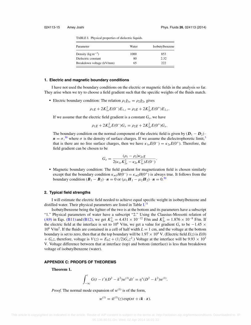
TABLE I. Physical properties of dielectric liquids.
Parameter Water Isobutylbenzene
Density (kg m−3) 1000 853Dielectric constant 80 2.32Breakdown voltage (kV/mm) 65 222
1. Electric and magnetic boundary conditions
I have not used the boundary conditions on the electric or magnetic fields in the analysis so far.They arise when we try to choose a field gradient such that the specific weights of the fluids match.
� Electric boundary condition: The relation ρ1g1e = ρ2g2e gives
ρ1g + 2K 21e E(0−)E1,z = ρ2g + 2K 2
2e E(0+)E2,z .
If we assume that the electric field gradient is a constant Ge, we have
ρ1g + 2K 21e E(0−)Ge = ρ2g + 2K 2
2e E(0+)Ge.
The boundary condition on the normal component of the electric field is given by (D1 − D2) ·n = σ ,30 where σ is the density of surface charges. If we assume the dielectrophoretic limit,3
that is there are no free surface charges, then we have κ1eE(0−) = κ2eE(0+). Therefore, thefield gradient can be chosen to be
Ge = (ρ1 − ρ2)κ2eg
2(κ1e K 22e − κ2e K 2
1e)E(0−).
� Magnetic boundary condition: The field gradient for magnetization field is chosen similarlyexcept that the boundary condition κm1H(0−) = κm2H(0+) is always true. It follows from theboundary condition (B1 − B2) · n = 0 or (μ1 H1 − μ2 H2) · n = 0.30
2. Typical field strengths
I will estimate the electric field needed to achieve equal specific weight in isobutylbenzene anddistilled water. Their physical parameters are listed in Table I.31
Isobutylbenzene being the lighter of the two is at the bottom and its parameters have a subscript“1.” Physical parameters of water have a subscript “2.” Using the Clausius-Mossotti relation of(A9) in Eqs. (B11) and (B12), we get K 2
1e = 4.431 × 10⁻¹² F/m and K 22e = 1.876 × 10⁻⁸ F/m. If
the electric field at the interface is set to 106 V/m, we get a value for gradient Ge to be −1.45 ×10⁶ V/m2. If the fluids are contained in a cell of half width L = 1 cm, and the voltage at the bottomboundary is set to zero, then that at the top boundary will be 1.97 × 10⁴ V. (Electric field E(z) is E(0)+ Gez, therefore, voltage is V (z) = E0z + (1/2)Gez2.) Voltage at the interface will be 9.93 × 10³
V. Voltage difference between that at interface (top) and bottom (interface) is less than breakdownvoltage of isobutylbenzene (water).
APPENDIX C: PROOFS OF THEOREMS
Theorem 1. ∫ t
−∞G(t − t ′)(D2 − k2)w(1)dt ′ = η∗(D2 − k2)w(1).
Proof. The normal mode expansion of w(1) is of the form,
w(1) = w(1)(z) exp(nt + i k · x).
This article is copyrighted as indicated in the article. Reuse of AIP content is subject to the terms at: http://scitation.aip.org/termsconditions. Downloaded to IP:
95.136.80.51 On: Wed, 02 Apr 2014 16:01:33
024113-16 Amey Joshi Phys. Fluids 26, 024113 (2014)
Therefore, the left hand side (LHS) becomes
L H S =∫ t
−∞G(t − t ′)(D2 − k2)w(1)(z) exp(nt ′ + i k · x)dt ′
= (D2 − k2)w(1)(z) exp(i k · x)∫ t
−∞G(t − t ′) exp(nt ′)dt ′.
A transformation s = t − t′ simplifies the integral to∫ t
−∞G(t − t ′) exp(nt ′)dt ′ = exp(nt)
∫ ∞
0G(s) exp(−ns)ds = exp(nt)η∗.
Therefore,
L H S = (D2 − k2)w(1)(z) exp(i k · x) exp(nt)η∗ = η∗(D2 − k2)w(1). (C1)
�
Theorem 2. For an eigenvalue ni of equation (36) we have
(n2i − (n∗
i )2)I3 = (n∗i η − niη
∗)I4, (C2)
where I3 > 0, I4 > 0 and
I3 =∫ d
0
{ρ(0)|w(1)
i |2 + ρ(0)
k2|Dw
(1)i |2
}dz, (C3)
I4 =∫ d
0
{k2|w(1)
i |2 + 2|Dw(1)i |2 + |D2w
(1)i |2
k2
}dz. (C4)
Proof. One form of Eq. (36) is
g∫ d
0w
(1)j w
(1)i Dρ(0)dz − k2γ
∫ d
0w
(1)j w
(1)i δ(z − z(0))dz =
n2i
∫ d
0
{ρ(0)wi
(1)w(1)j + ρ(0)
k2Dw
(1)i Dw
(1)j
}dz+
niη∗∫ d
0
{k2w
(1)i w
(1)j + 2Dw
(1)i Dw
(1)j + (D2w
(1)i )(D2w
(1)j )
k2
}dz.
(C5)
Interchanging i and j,
g∫ d
0w
(1)j w
(1)i Dρ(0)dz − k2γ
∫ d
0w
(1)j w
(1)i δ(z − z(0))dz =
n2j
∫ d
0
{ρ(0)wi
(1)w(1)j + ρ(0)
k2Dw
(1)i Dw
(1)j
}dz+
n jη∗∫ d
0
{k2w
(1)i w
(1)j + 2Dw
(1)i Dw
(1)j + (D2w
(1)i )(D2w
(1)j )
k2
}dz.
(C6)
This article is copyrighted as indicated in the article. Reuse of AIP content is subject to the terms at: http://scitation.aip.org/termsconditions. Downloaded to IP:
95.136.80.51 On: Wed, 02 Apr 2014 16:01:33
024113-17 Amey Joshi Phys. Fluids 26, 024113 (2014)
If n j = n∗i , then
g∫ d
0|w(1)
i |2 Dρ(0)dz − k2γ
∫ d
0|w(1)
i |2δ(z − z(0))dz =
(n∗i )2
∫ d
0
{ρ(0)|w(1)
i |2 + ρ(0)
k2|Dw
(1)i |2
}dz+
n∗i η
∫ d
0
{k2|w(1)
i |2 + 2|Dw(1)i |2 + |D2w
(1)i |2
k2
}dz.
(C7)
Under the same assumptions, Eq. (C5) becomes
g∫ d
0|w(1)
i |2 Dρ(0)dz − k2γ
∫ d
0|w(1)
i |2δ(z − z(0))dz =
(ni )2∫ d
0
{ρ(0)|w(1)
i |2 + ρ(0)
k2|Dw
(1)i |2
}dz+
niη∗∫ d
0
{k2|w(1)
i |2 + 2|Dw(1)i |2 + |D2w
(1)i |2
k2
}dz.
(C8)
Subtracting Eq. (C7) from Eq. (C8),
(n2i − (n∗
i )2)∫ d
0
{ρ(0)|w(1)
i |2 + ρ(0)
k2|Dw
(1)i |2
}dz =
(n∗i η − niη
∗)∫ d
0
{k2|w(1)
i |2 + 2|Dw(1)i |2 + |D2w
(1)i |2
k2
}dz. (C9)
The integrands in the above equation are positive definite and so are the limits, therefore the integralsthemselves are positive. We can write Eq. (C9) in a simpler form as
(n2i − (n∗
i )2)I3 = (n∗i η − niη
∗)I4, (C10)
where I3 > 0, I4 > 0 and
I3 =∫ d
0
{ρ(0)|w(1)
i |2 + ρ(0)
k2|Dw
(1)i |2
}dz, (C11)
I4 =∫ d
0
{k2|w(1)
i |2 + 2|Dw(1)i |2 + |D2w
(1)i |2
k2
}dz. (C12)
�Theorem 3. For an eigenvalue ni of Eq. (36) we have
(n∗i − ni )I5 +
(g
ni− g
n∗i
)I6 −
(k2γ
ni− k2γ
n∗i
)I7 = 0, (C13)
This article is copyrighted as indicated in the article. Reuse of AIP content is subject to the terms at: http://scitation.aip.org/termsconditions. Downloaded to IP:
95.136.80.51 On: Wed, 02 Apr 2014 16:01:33
024113-18 Amey Joshi Phys. Fluids 26, 024113 (2014)
where
I5 =∫ d
0
{ρ(0)|w(1)
i |2 + ρ(0)
k2|Dw
(1)i |2
}dz > 0, (C14)
I6 =∫ d
0|w(1)
i |2 Dρ(0)dz, (C15)
I7 =∫ d
0|w(1)
i |2δ(z − z(0))dz > 0. (C16)
Proof. Proof of Theorem 2 involved manipulating a form of Eq. (36). If we continue with thatequation in its original form and interchange i and j, we get
−n j
∫ d
0
{ρ(0)w
(1)j w
(1)i + ρ(0)
k2Dw
(1)j Dw
(1)i
}dz + g
n j
∫ d
0w
(1)i w
(1)j Dρ(0)dz
−k2γ
n j
∫ d
0w
(1)i w
(1)j δ(z − z(0))dz =
η∗∫ d
0
{k2w
(1)j w
(1)i + 2Dw
(1)j Dw
(1)i + x
k2(D2w
(1)j )(D2w
(1)i )
}dz.
(C17)
Subtracting it from Eq. (36), we get
(n j − ni )∫ d
0
{ρ(0)w
(1)j w
(1)i + ρ(0)
k2Dw
(1)j Dw
(1)i
}dz+
(g
ni− g
n j
)∫ d
0w
(1)i w
(1)j Dρ(0)dz−
(k2γ
ni− k2γ
n j
) ∫ d
0w
(1)i w
(1)j δ(z − z(0))dz = 0. (C18)
If we now choose n j = n∗i , we can write Eq. (C18) as
(n∗i − ni )I5 +
(g
ni− g
n∗i
)I6 −
(k2γ
ni− k2γ
n∗i
)I7 = 0, (C19)
where
I5 =∫ d
0
{ρ(0)|w(1)
i |2 + ρ(0)
k2|Dw
(1)i |2
}dz > 0, (C20)
I6 =∫ d
0|w(1)
i |2 Dρ(0)dz, (C21)
I7 =∫ d
0|w(1)
i |2δ(z − z(0))dz > 0. (C22)
This article is copyrighted as indicated in the article. Reuse of AIP content is subject to the terms at: http://scitation.aip.org/termsconditions. Downloaded to IP:
95.136.80.51 On: Wed, 02 Apr 2014 16:01:33
024113-19 Amey Joshi Phys. Fluids 26, 024113 (2014)
The sign of I6 depends on the density gradient. It is positive if density increases with increasingz and is negative if density decreases with increasing z. We can simplify (C19) to get
(n∗i − ni )
(I5 + g I6
|ni |2 − k2γ I7
|ni |2)
= 0. (C23)
�
1. Descartes rule of signs
Descartes rule of signs32 is
1. If the terms of a single-variable polynomial with real coefficients are ordered by descendingvariable exponent, then the number of positive roots of the polynomial is either equal to thenumber of sign differences between consecutive nonzero coefficients, or is less than it by aneven number. Multiple roots of the same value are counted separately.
2. As a corollary of the point 1, the number of negative roots is the number of sign changes aftermultiplying the coefficients of odd-power terms by 1, or fewer than it by a multiple of 2.
1 J. W. Strutt, “Investigation of the character of the equilibrium of an incompressible heavy fluid of variable density,” Proc.London Math. Soc. s1-14, 170–177 (1882).
2 G. I. Taylor, “The instability of liquid surfaces when accelerated in a direction perpendicular to their plane,” Proc. R. Soc.(London) A 201, 192–196 (1950).
3 A. Joshi, M. Radhakrishna, and N. Rudraiah, “Rayleigh-Taylor instability in dielectric fluids,” Phys. Fluids 22, 064102(2010).
4 H. Geisekus, “Zur stabilitat von stromungen viskoelastischer flussigkeiten-1. ebene and kreisformige couette-stromung,”Rheol. Acta 5, 239 (1966).
5 S. H. Muller, R. G. Larson, and E. S. G. Shaqfeh, “A purely elastic transition in Taylor-Couette flow,” Rheol. Acta 28,499–503 (1989).
6 Y. Renardy, “Stability of the interface in two-layer Couette flow of upper convected Maxwell liquids,” J. Non-NewtonianFluid Mech. 28, 99–115 (1988).
7 Y.-Y. Su and B. Khomami, “Interfacial stability of multilayer viscoelastic fluids in slit and converging channel diegeometries,” J. Rheol. 36, 357 (1992).
8 Y. Su and B. Khomami, “Purely elastic interfacial instabilities in superposed flow of polymeric fluids,” Rheol. Acta 31,413–420 (1992).
9 B. Suman and S. Kumar, “Surfactant and elasticity induced inertialess instabilities in vertically vibrated liquids,” J. FluidMech. 610, 407–423 (2008).
10 L. Aitken and S. Wilson, “Rayleigh-Taylor instability in elastic liquids,” J. Non-Newtonian Fluid Mech. 49, 13–22(1993).
11 A. Saasen and P. A. Tyvand, “Rayleigh-Taylor instability and Rayleigh-type waves on a Maxwell-fluid,” Z. Angew. Math.Phys. 41, 284–293 (1990).
12 A. Saasen and O. Hassager, “Gravity waves and Rayleigh Taylor instability on a Jeffrey-fluid,” Rheol. Acta 30, 301–306(1991).
13 A. R. Piriz, J. J. L. Cela, O. D. Cortazar, N. A. Tahir, and D. H. H. Hoffmann, “Rayleigh-Taylor instability in elastic solids,”Phys. Rev. E 72, 056313 (2005).
14 G. Dimonte, “Nonlinear evolution of the Rayleigh-Taylor and Richtmyer-Meshkov instabilities,” Phys. Plasmas 6, 2009(1999).
15 D. Joseph, G. Beavers, and T. Funada, “Rayleigh-Taylor instability of viscoelastic drops at high Weber numbers,” J. FluidMech. 453, 109–132 (2002).
16 D. D. Joseph, J. Belanger, and G. Beavers, “Breakup of a liquid drop suddenly exposed to a high-speed airstream,” Int. J.Multiphase Flow 25, 1263–1303 (1999).
17 R. B. Bird, R. C. Armstrong, and O. Hassager, Dynamics of Polymeric Liquids (John Wiley & Sons Inc, 1977), Vol. 1,p. 263.
18 S. Chandrasekhar, Hydrodynamic and Hydromagnetic Stability, International Series of Monographs on Physics Vol. 1(Clarendon, Oxford, 1961).
19 R. B. Bird, R. C. Armstrong, and O. Hassager, Dynamics of Polymeric Liquids (John Wiley & Sons Inc, 1977), Vol. 1,pp. 264–265.
20 A. S. Joshi, M. Radhakrishna, and N. Rudraiah, “Kelvin-Helmholtz instability in viscoelastic fluids in presence of electro-magnetic fields,” Phys. Fluids 23, 094107 (2011).
21 G. K. Batchelor, An Introduction to Fluid Dynamics (Cambridge University Press, 2000), pp. 63–64.22 I. S. Gradshteyn and I. M. Ryzhik, Tables of Integrals, Series, and Products, 6th ed. (Academic Press, San Diego, CA,
2000), p. 1076.23 L. D. Landau, E. M. Lifshitz, and L. P. Pitaevskii, Electrodynamics of Continuous Media, 1st Indian reprint ed. (Butterworth-
Heinemann, Oxford, UK, 2005), Eq. (15.7), p. 61.
This article is copyrighted as indicated in the article. Reuse of AIP content is subject to the terms at: http://scitation.aip.org/termsconditions. Downloaded to IP:
95.136.80.51 On: Wed, 02 Apr 2014 16:01:33
024113-20 Amey Joshi Phys. Fluids 26, 024113 (2014)
24 J. D. Jackson, Classical Electrodynamics, 3rd ed. (John Wiley & Sons (Asia) Pte Ltd., Singapore, 1999), pp. 258–262.25 E. Schaffer, T. Thurn-Albrecht, T. P. Russell, and U. Steiner, “Electrohydrodynamic instabilities in polymer films,”
Europhys. Lett. 53, 518 (2001).26 L. D. Landau, E. M. Lifshitz, and L. P. Pitaevskii, Electrodynamics of Continuous Media, 1st Indian reprint ed. (Butterworth-
Heinemann, Oxford, UK, 2005), Eq. (15.11), p. 62.27 W. K. H. Panofsky and M. Phillips, Classical Electricity and Magnetism, 2nd ed. (Dover Publications, New York, 1955),
p. 39.28 A. Rai-Choudhuri, The Physics of Fluids and Plasmas: An Introduction for Astrophysicists (Cambridge University Press,
1998), pp. 141–145.29 H. Lamb, Hydrodynamics, 6th ed. (Cambridge University Press, 1932).30 J. D. Jackson, Classical Electrodynamics, 3rd ed. (John Wiley & Sons (Asia) Pte Ltd., Singapore, 1999), p. 18.31 CRC Handbook of Physics and Chemistry, 90th ed., edited by D. R. Lide (CRC Press, Boca Raton, FL, 2009).32 X. Wang, “A simple proof of Descartes’s rule of signs,” Am. Math. Mon. 111, 525–526 (2004).
This article is copyrighted as indicated in the article. Reuse of AIP content is subject to the terms at: http://scitation.aip.org/termsconditions. Downloaded to IP:
95.136.80.51 On: Wed, 02 Apr 2014 16:01:33