Technical Report Documentation Page 1. Report No. FHWA/TX-03/0-2107-1

2. Government Accession No.

3. Recipient's Catalog No.

4. Title and Subtitle EL PASO TRANSIMS CASE STUDY

5. Report Date April 2003

6. Performing Organization Code

7. Author(s) Larry Rilett, Akshit Kumar, and Srikar Doddi

8. Performing Organization Report No. Report 0-2107-1 10. Work Unit No. (TRAIS)

9. Performing Organization Name and Address Texas Transportation Institute The Texas A&M University System College Station, Texas 77843-3135

11. Contract or Grant No. Project No. 0-2107 13. Type of Report and Period Covered Research: September 2000 – August 2001

12. Sponsoring Agency Name and Address Texas Department of Transportation Research and Technology Implementation Office P. O. Box 5080 Austin, Texas 78763-5080

14. Sponsoring Agency Code

15. Supplementary Notes Research performed in cooperation with the Texas Department of Transportation and the U.S. Department of Transportation, Federal Highway Administration. Research Project Title: Mobile Source Emission Modeling: Methods, Sensitivity, and Analysis of Assumptions 16. Abstract The Transportation Analysis and Simulation System (TRANSIMS), which was developed as part of the Travel Model Improvement Program (TMIP), has been touted by its backers as a replacement for the four-step planning model. TRANSIMS is an integrated system of travel forecasting models which is designed to give transportation planners accurate, complete information on traffic impacts, congestion, and pollutant emissions. Because TRANSIMS represents a significant shift from the current state of practice, the transportation planning community will need to spend significant human and capital resources preparing for the transition. This report will provide some insight into these transitional issues based on research on the El Paso planning network in Texas. This report is comprised of three main sections. First the report provides a detailed overview of the TRANSIMS architecture. It is subsequently compared and contrasted with the four-step planning process. The next section describes the detailed data requirements, provides a description of the steps taken to create a TRANSIMS network for El Paso, and discusses the microsimulation results. Because TRANSIMS 1.1, which was used in this research, did not contain all the modules the research primarily focused on the microsimulation and emissions modules. Lastly, the TRANSIMS emission estimation process is described. Subsequently, this module is compared and contrasted to the MOBILE5 suite of emissions models. A “lessons learned” section is provided at the end of each section outlining the important findings. 17. Key Words TRANSIMS, Emissions, Four-Step Model

18. Distribution Statement No restrictions. This document is available to the public through NTIS: National Technical Information Service 5285 Port Royal Road Springfield, Virginia 22161

19. Security Classif.(of this report) Unclassified

20. Security Classif.(of this page) Unclassified

21. No. of Pages 98

22. Price

Form DOT F 1700.7 (8-72) Reproduction of completed page authorized

EL PASO TRANSIMS CASE STUDY

by

Larry Rilett Associate Research Engineer Texas Transportation Institute

Akshit Kumar

Graduate Assistant Researcher Texas Transportation Institute

Srikar Doddi

Graduate Assistant Researcher Texas Transportation Institute

Product 2107-1 Project Number 0-2107

Research Project Title: Mobile Source Emission Modeling: Methods, Sensitivity, and Analysis of Assumptions

Sponsored by the Texas Department of Transportation

In Cooperation with the U.S. Department of Transportation Federal Highway Administration

April 2003

TEXAS TRANSPORTATION INSTITUTE The Texas A&M University System College Station, Texas 77843-3135

v

DISCLAIMER

The contents of this report reflect the views of the authors, who are responsible for the

facts and the accuracy of the data presented herein. The contents do not necessarily reflect the

official view or policies of the Federal Highway Administration (FHWA) or the Texas

Department of Transportation (TxDOT). This report does not constitute a standard, specification,

or regulation. The United States Government and the State of Texas do not endorse products or

manufacturers. Trade or manufacturers’ names appear herein solely because they are considered

essential to the object of this report. Larry R. Rilett, Ph.D., was the research supervisor for this

project.

vi

ACKNOWLEDGMENTS

The research team would like to acknowledge the cooperation of individuals at the Texas

Department of Transportation as well as individuals with state and local agencies who assisted in

the development of this report, from data collection to final review. The team also acknowledges

the Federal Highway Administration and the Texas Department of Transportation as sponsors of

this research project. Additionally, the research team acknowledges the guidance and assistance

of the project director, Mr. Mark Hodges of the Texas Department of Transportation. This

project was conducted in cooperation with TxDOT and FHWA.

vii

TABLE OF CONTENTS

Page LIST OF FIGURES ..................................................................................................................... viii LIST OF TABLES.......................................................................................................................... x CHAPTER ONE—INTRODUCTION........................................................................................ 1-1 CHAPTER TWO—TRANSPORTATION ANALYSIS AND SIMULATION SYSTEM (TRANSIMS)................................................................................................................... 2-1 2.1 Overview of TRANSIMS ....................................................................................... 2-1 2.2 Comparison of TRANSIMS with the Four-Step Model ......................................... 2-4

2.3 Traffic Microsimulation.......................................................................................... 2-7 2.3.1 Traditional Supply Relationships.................................................................. 2-7 2.3.2 TRANSIMS Supply Relationship................................................................. 2-8 2.3.3 Fundamental Properties of TRANSIMS..................................................... 2-12 2.3.4 Modeling Interrupted Flow Facilities ......................................................... 2-18 2.3.5 Analysis of Output ...................................................................................... 2-19

2.4 Lessons Learned.................................................................................................... 2-22 CHAPTER THREE—THE EL PASO CASE STUDY............................................................... 3-1 3.1 Methodology........................................................................................................... 3-1 3.2 El Paso Network Conversion .................................................................................. 3-4

3.2.1 Node and Link Information Conversion ....................................................... 3-6 3.2.2 Traffic Signal Control ................................................................................. 3-14

3.3 El Paso Case Study Demand Conversion ............................................................. 3-17 3.4 El Paso Microsimulation Results .......................................................................... 3-19 3.5 Lessons Learned.................................................................................................... 3-25 CHAPTER FOUR—EMISSIONS ESTIMATION ..................................................................... 4-1 4.1 TRANSIMS Emissions Estimator Module............................................................. 4-1

4.1.1 Fleet Composition......................................................................................... 4-2 4.1.2 Fleet Status.................................................................................................... 4-3 4.1.3 Fleet Dynamics ............................................................................................. 4-6

4.2 The MOBILE5a Emissions Model ....................................................................... 4-14 4.3 Comparison between TRANSIMS and MOBILE5a Emissions Rates ................. 4-21 4.4 El Paso Case Study Results .................................................................................. 4-23 4.5 Lessons Learned.................................................................................................... 4-33 REFERENCES ............................................................................................................................ 5-1

viii

LIST OF FIGURES Figure Page 2.1 TRANSIMS Architecture ................................................................................................ 2-2 2.2 Comparison of Four-Step and TRANSIMS Architecture................................................ 2-5 2.3 Sample Speed-Time Plot for an Individual Vehicle ...................................................... 2-11 2.4 Free Flow Speed versus Parameter pnoise ....................................................................... 2-14 2.5 Speed versus Flow for Different Aggregation Intervals for I-10 Corridor in Houston, Texas .............................................................................................................. 2-16 2.6 Speed versus Flow for Different pnoise Values for I-10 Corridor in Houston, Texas .............................................................................................................. 2-17 2.7a Contour Plot of Speed on North Dallas Tollway, Dallas, Texas (pnoise = 0.2) ............... 2-21 2.7b Contour Plot of Speed on North Dallas Tollway, Dallas, Texas (pnoise = 0.3) ............... 2-21 3.1 Modification of TRANSIMS Architecture ...................................................................... 3-2 3.2 Study Methodology.......................................................................................................... 3-3 3.3 El Paso, Texas, Network.................................................................................................. 3-5 3.4 Downtown El Paso, Texas, Network ............................................................................... 3-5 3.5 Schematic Diagram of a Pocket Lane.............................................................................. 3-9 3.6 Lane Connectivity Example........................................................................................... 3-12 3.7 Turning Movement Example ......................................................................................... 3-13 3.8 El Paso Functional Classification Histogram ................................................................ 3-21 3.9 El Paso Network Length by Functional Classification .................................................. 3-21 3.10 Number of Completed Trips versus Iteration Number .................................................. 3-22 3.11 Total Travel Time by Functional Classification ............................................................ 3-24 4.1 Light-Duty Vehicle Emissions Estimation Methodology................................................ 4-2 4.2 Emissions Multiplier for One Hour Soak Time by Start/Stop Cycle............................... 4-5 4.3 Power versus Speed Bin................................................................................................... 4-9 4.4 Fuel Consumption Rate versus Speed Bin..................................................................... 4-10 4.5 NOx Emissions Rate versus Speed Bin ......................................................................... 4-11 4.6 CO Emissions Rate versus Speed Bin ........................................................................... 4-11 4.7 HC Emissions Rate versus Speed Bin ........................................................................... 4-12 4.8 El Paso Vehicle Mix for MOBILE5a Vehicle Categories ............................................. 4-20 4.9 El Paso MOBILE5a CO Emissions Rate versus Speed ................................................. 4-20 4.10 El Paso MOBILE5a NOx Emissions Rate versus Speed............................................... 4-21 4.11 Comparison between CO Emissions Rates for TRANSIMS and MOBILE5a.............. 4-22 4.12 Comparison between NOx Emissions Rates for TRANSIMS and MOBILE5a............ 4-23 4.13 El Paso Case Study Estimated System Emissions ......................................................... 4-24 4.14 Estimated CO Emissions by Functional Classification ................................................. 4-25 4.15 Estimated NOx Emissions by Functional Classification ............................................... 4-25 4.16 Estimated HC Emissions by Functional Classification ................................................. 4-26 4.17 Estimated Fuel Consumption by Functional Classification........................................... 4-27 4.18 Comparison of Estimated CO Emissions from TRANSIMS and MOBILE5a.............. 4-28 4.19 Comparison of Estimated NOx Emissions from TRANSIMS and MOBILE5a............ 4-29

ix

4.20 Speed versus Box Number for Arterial Link 4607 ........................................................ 4-30 4.21 CO Emissions versus Box Number for Arterial Link 4607........................................... 4-31 4.22 NOx Emissions versus Box Number for Arterial Link 4607......................................... 4-32

x

LIST OF TABLES Table Page

2.1 Maximum Link Speed (miv ) Conversion Table ............................................................... 2-9

3.1 Required El Paso TRANSIMS Files................................................................................ 3-6 3.2 Node File.......................................................................................................................... 3-7 3.3 Link File........................................................................................................................... 3-8 3.4 Pocket Lane File ............................................................................................................ 3-10 3.5 Lane Connectivity File................................................................................................... 3-14 3.6 Unsignalized Intersection File ....................................................................................... 3-15 3.7 Signalized Intersection File............................................................................................ 3-15 3.8 Signal Timing File ......................................................................................................... 3-16 3.9 Traffic Signal Phasing File ............................................................................................ 3-17 3.10 Parking File.................................................................................................................... 3-18 3.11 Study Area File .............................................................................................................. 3-18 3.12 El Paso Functional Classification .................................................................................. 3-20 4.1 Vehicle Categories ........................................................................................................... 4-3 4.2 Link to Velocity Summary File ....................................................................................... 4-6

1-1

CHAPTER 1–INTRODUCTION

It has long been recognized that the traditional four-step travel demand model is not

robust enough to analyze adequately many of the issues facing transportation planners.

Sustainable development, environmental impacts of proposed projects, and Intelligent

Transportation Systems (ITS) deployment are examples of some current topics of interest. One

potential solution has been to adopt stochastic, microscopic based models that can model

individual demand responses to changes in supply. One of the most comprehensive of these

models is the Transportation Analysis and Simulation System (TRANSIMS) which was

developed as part of the Travel Model Improvement Program (TMIP) (Weiner and Ducca,

1999). Because TRANSIMS represents a significant shift from the current state of the practice,

the transportation planning community will need to spend significant human and capital

resources preparing for the transition. This report will provide some insight into these

transitional issues based on research on the El Paso planning network in Texas.

TRANSIMS is an integrated system of travel forecasting models that is designed to give

transportation planners accurate, complete information on traffic impacts, congestion, and

pollution. The underlying philosophy of the approach is to model individual travelers and their

behavior. It was created at Los Alamos National Laboratory (LANL) under the sponsorship of

the U.S. Department of Transportation, the Environmental Protection Agency (EPA), and the

Department of Energy. The general approach is to create a virtual metropolitan region which

includes a complete representation of a region’s individuals, activities, and transportation

infrastructure. The individuals plan their trips to satisfy their desired activity patterns. The

movements of every individual in the metropolitan area across all modes of the transportation

systems are simulated on a second-by-second basis. The goal is to produce realistic traffic

dynamics so that users can obtain accurate vehicle pollutant emissions and fuel consumption

estimates. Similar to the four-step transportation model TRANSIMS is a sequential (not

simultaneous) model which means that there is an explicit feedback loop whereby the individual

travelers’ reactions to information about the satisfaction of their preferences is modeled.

TRANSIMS consists of five modules: a population synthesizer, an activity generator, a trip

planner, a traffic microsimulation and an emissions estimator. This project was conducted using

1-2

TRANSIMS 1.0 and TRANSIMS 1.1, and because these versions consist primarily of the traffic

microsimulation and emissions estimator, the researcher primarily focused on these modules.

The report is divided into four chapters. The second chapter provides a detailed overview

of the TRANSIMS architecture. Subsequently the architecture of the traditional four-step

planning model is compared and contrasted with the TRANSIMS architecture. The third chapter

consists of two sections. The first section describes the creation of the supply and demand files

for TRANSIMS. With respect to the supply information the basic strategy was to use as much

information from the existing planning network as possible. A number of heuristics were created

to populate the network with information, such as traffic signal locations and signal timing plans,

that was unattainable. The demand information was translated from the TRANPLAN

origin/destination (OD) matrix. Because TRANSIMS does not use zones the zonal movements

were translated into individual trips to and from parking lots located on links throughout the

zone. The second section describes the feedback methodology and presents the final

microsimulation results. A number of sensitivity analyses were conducted. Chapter 4 examines

the emissions estimation process. The first section describes the emissions model for

TRANSIMS and the required input. The model is compared and contrasted to the MOBILE5

emissions model which is the state of practice in most of the United States, including Texas. The

emissions are subsequently calculated for the El Paso network using both approaches. A

“lessons learned” section is provided at the end of each chapter.

2-1

CHAPTER 2–TRANSPORTATION ANALYSIS AND SIMULATION SYSTEM

This chapter is divided into two sections. The first section provides an overview of the

TRANSIMS architecture. Subsequently, the TRANSIMS methodology is compared and

contrasted to the traditional four-step model. The second section provides a detailed description

of the traffic microsimulation module. The fundamental properties are described and the

importance of calibration is illustrated. Particular focus is provided on describing the changes

transportation planners will encounter if microsimulation approaches are adopted for long-term

planning.

2.1 OVERVIEW OF TRANSIMS

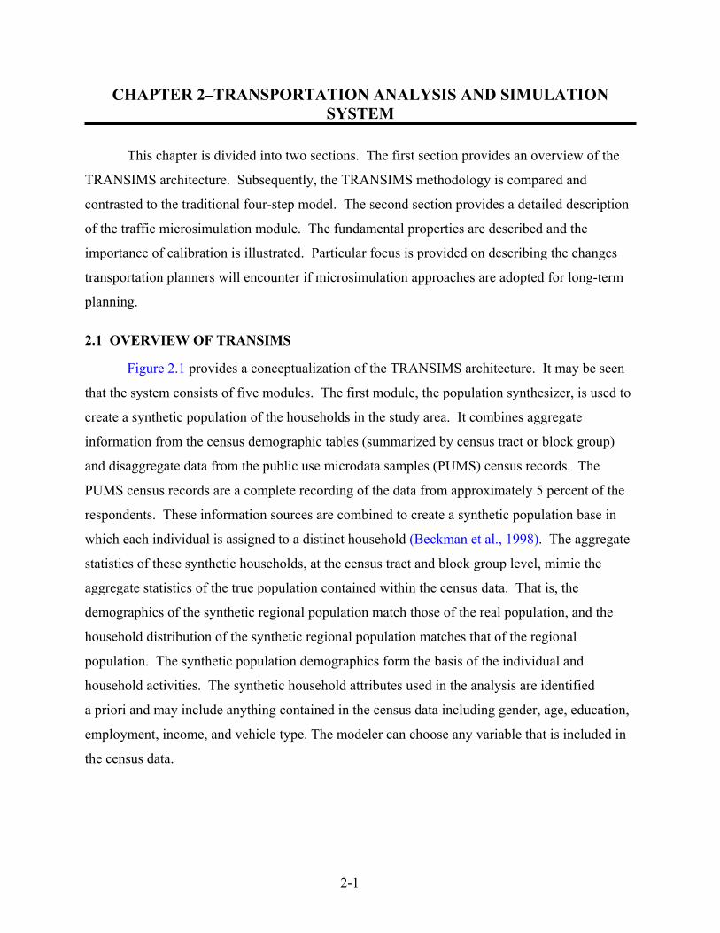
Figure 2.1 provides a conceptualization of the TRANSIMS architecture. It may be seen

that the system consists of five modules. The first module, the population synthesizer, is used to

create a synthetic population of the households in the study area. It combines aggregate

information from the census demographic tables (summarized by census tract or block group)

and disaggregate data from the public use microdata samples (PUMS) census records. The

PUMS census records are a complete recording of the data from approximately 5 percent of the

respondents. These information sources are combined to create a synthetic population base in

which each individual is assigned to a distinct household (Beckman et al., 1998). The aggregate

statistics of these synthetic households, at the census tract and block group level, mimic the

aggregate statistics of the true population contained within the census data. That is, the

demographics of the synthetic regional population match those of the real population, and the

household distribution of the synthetic regional population matches that of the regional

population. The synthetic population demographics form the basis of the individual and

household activities. The synthetic household attributes used in the analysis are identified

a priori and may include anything contained in the census data including gender, age, education,

employment, income, and vehicle type. The modeler can choose any variable that is included in

the census data.

2-2

Figure 2.1. TRANSIMS Architecture.

The second module, the household activity generator, identifies the set of “potential”

daily activities of each synthetic individual in each of the synthetic households. The input to this

module is the synthetic household population, a regional activity survey, and the network data

(both activity locations/land use and transportation network). The activity travel survey must

have a 24-hour or longer duration, be representative of the population, and include all activities

and trips of each member of the household. At the completion of this step the daily activities for

each member of each synthetic household are identified. The total number of trips each

individual is scheduled to complete can be obtained by counting the number of location changes

in their daily list of activities. In essence, the list of activities defines the daily trip chain(s)

desired by each traveler in the population and would be analogous to the information contained

in a traditional travel diary. For illustration purposes, a distinction is made in Figure 2.1 between

the list of activities and the activity attributes. The attributes of the activities would normally

include such things as activity priority, start time, duration, constraints, mode preference, and

possible locations.

The third module, the route planner, identifies the transportation routes for each trip

output from the second module in order to meet the individual travelers’ goals. Note that the

route attributes in the TRANSIMS context include not only what links a traveler would use but

also information such as mode, changes in mode, parking locations, and traveling companions.

5) Emissions Estimation

4) Microsimulation

3) Route Planner

1) Population Synthesizer (Generation of Synthetic Population)

2) Activity Generator Activities Activity Attributes

A B C

2-3

The input to the process includes traveler information and activity information from module 2 as

well as network information. Network information would include link location, link travel times

for each mode, mode accessibility, and so on. Note that all of the information associated with

each route (i.e., departure time, links used by mode, expected travel time, etc.) for each trip is

enumerated and output explicitly. In other words, the output from the route planner is a

complete enumeration of the transportation demand by mode and disaggregated by time of

departure.

The fourth module, the microsimulation, uses the route plans from module 3 as input and

simulates the transportation network at a microscopic level of detail, albeit at a lower fidelity

than most traffic operations models (LANL, 1998). In effect, module 4 simulates the interaction

between demand (the synthetic population’s desire to travel between activity locations) and

supply (the ability of the transportation system to meet this demand) for each mode over the

entire simulation period. In other words, the entire 24-hour transportation system dynamics are

modeled. As would be expected, the network data for each mode is a required input. The output

of the microsimulation module can be aggregated to any desired level. For example, it is

possible to obtain information on each traveler on a second-by-second basis. Alternatively, the

data may be aggregated both spatially (sub-link level to total network) and temporally (1 second

to 24-hour period) depending on the wishes of the modeler.

Once a TRANSIMS simulation is complete, the output from the microsimulation is used

to calculate various measures of effectiveness. Because the module is microsimulation-based

and every traveler and vehicle is modeled explicitly, the user has considerable flexibility in

choosing which metrics to use. Note that while the vehicles are modeled at a microscopic level

of detail, their emissions are not estimated within the microsimulation module. They are

estimated instead from the aggregate output data as shown in module 5 in Figure 2.1. The

developers adopted this approach because the microsimulation module is based on cellular

automata (CA) rules, which will be discussed in detail in the following sections. The important

point is that while TRANSIMS has been calibrated to macroscopic flow observations there is no

guarantee that the microscopic speed profiles are accurate or even reasonable (Nagel et al., 1997;

Williams et al., 1999; Zietsman and Rilett, 2001). Therefore, the individual vehicle speed

profiles, and associated accelerations and decelerations cannot be used for calculating vehicle

emissions.

2-4

Because of the inherent complexity associated with demand estimation, TRANSIMS

models the traveler’s decision making, an inherently simultaneous process, in a sequential

manner with appropriate feedback loops. For example, in order to identify accurately a traveler’s

activities or plans (i.e., module 2), the level of service (LOS) attributes, such as travel time, of

the different modes by time of day need to be known. The attributes will clearly not be known

until the microsimulation module (i.e., module 4) is complete. Therefore, during the first

iteration the LOS values are estimated. If the estimated LOS values and the resulting output

LOS values do not match, then the user makes adjustments and repeats the process as shown in

Figure 2.1. That is, the simulated activities as defined by arrow A, the activity attributes

(location, time, etc.) as defined by arrow B, and the routes (departure time, links used, etc.) as

defined by arrow C may be changed as a result of new LOS values output from the

microsimulation module. It is important to note that the feedback can take place in a variety of

ways. The optimal configuration of the iterations or feedback loops and the conditions, if any,

under which this process converges, are ongoing research topics (Smith et al., 2000).

2.2 COMPARISON OF TRANSIMS WITH THE FOUR-STEP MODEL

Because of the long history of the four-step model in transportation planning, there is a

natural tendency to discuss TRANSIMS using traditional planning terminology. In one sense

this is reasonable because the underlying conceptualization of the transportation demand/supply

process for both approaches is essentially the same. In addition, while the underlying process is

simultaneous in nature both approaches are iterative as evidenced by the feedback steps

associated with them. However, a direct comparison is problematic because TRANSIMS

represents a fundamental shift, rather than an incremental change, in the implementation of the

underlying conceptualization.

Obviously the key difference between the approaches is that TRANSIMS is

microsimulation based and is therefore capable of modeling the stochastic and dynamic attributes

of the transportation system. Each traveler’s activities, for example, are considered across the

entire day as a single entity or chain. Thus all of the major lifestyle and travel decisions such as

what activities to participate in, when to participate in the activities, where to participate, what

mode to use, or what route to choose can be made in a consistent manner at the individual

traveler level. This ability is not remotely possible with the macroscopic four-step model. In

2-5

addition, because TRANSIMS is stochastic, the LOS values can have confidence and/or

tolerance intervals associated with them. In contrast, the four-step model tends to have varying

levels of detail at each step. For example, traditionally trip distribution is aggregate and mode

choice is disaggregate, and the four steps are basically treated independently of each other.

Therefore, the ability to model decisions consistently and at a disaggregate level across all four

steps and to put confidence bounds on the resulting estimates is problematic, at best, for the

macroscopic four-step model.

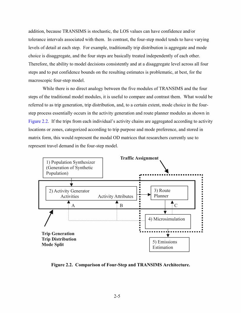
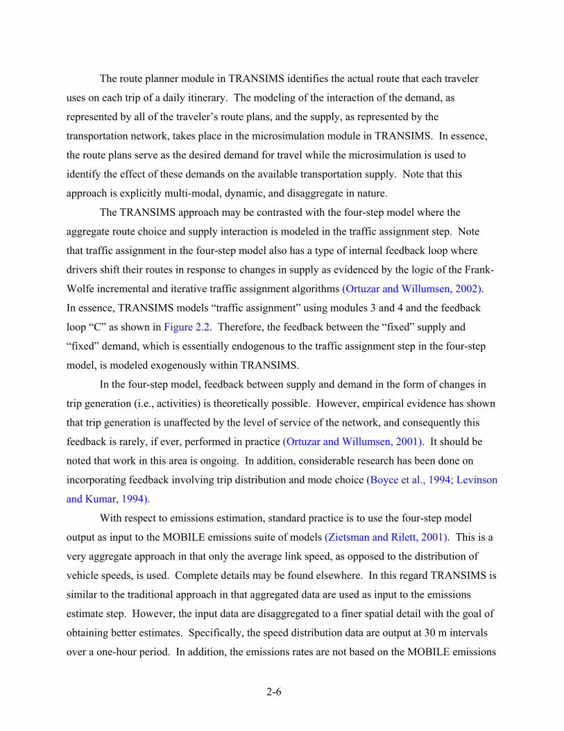
While there is no direct analogy between the five modules of TRANSIMS and the four

steps of the traditional model modules, it is useful to compare and contrast them. What would be

referred to as trip generation, trip distribution, and, to a certain extent, mode choice in the four-

step process essentially occurs in the activity generation and route planner modules as shown in

Figure 2.2. If the trips from each individual’s activity chains are aggregated according to activity

locations or zones, categorized according to trip purpose and mode preference, and stored in

matrix form, this would represent the modal OD matrices that researchers currently use to

represent travel demand in the four-step model.

Figure 2.2. Comparison of Four-Step and TRANSIMS Architecture.

5) Emissions Estimation

4) Microsimulation

3) Route Planner

1) Population Synthesizer (Generation of Synthetic Population)

2) Activity Generator Activities Activity Attributes

A

B C

Traffic Assignment

Trip Generation Trip Distribution Mode Split

2-6

The route planner module in TRANSIMS identifies the actual route that each traveler

uses on each trip of a daily itinerary. The modeling of the interaction of the demand, as

represented by all of the traveler’s route plans, and the supply, as represented by the

transportation network, takes place in the microsimulation module in TRANSIMS. In essence,

the route plans serve as the desired demand for travel while the microsimulation is used to

identify the effect of these demands on the available transportation supply. Note that this

approach is explicitly multi-modal, dynamic, and disaggregate in nature.

The TRANSIMS approach may be contrasted with the four-step model where the

aggregate route choice and supply interaction is modeled in the traffic assignment step. Note

that traffic assignment in the four-step model also has a type of internal feedback loop where

drivers shift their routes in response to changes in supply as evidenced by the logic of the Frank-

Wolfe incremental and iterative traffic assignment algorithms (Ortuzar and Willumsen, 2002).

In essence, TRANSIMS models “traffic assignment” using modules 3 and 4 and the feedback

loop “C” as shown in Figure 2.2. Therefore, the feedback between the “fixed” supply and

“fixed” demand, which is essentially endogenous to the traffic assignment step in the four-step

model, is modeled exogenously within TRANSIMS.

In the four-step model, feedback between supply and demand in the form of changes in

trip generation (i.e., activities) is theoretically possible. However, empirical evidence has shown

that trip generation is unaffected by the level of service of the network, and consequently this

feedback is rarely, if ever, performed in practice (Ortuzar and Willumsen, 2001). It should be

noted that work in this area is ongoing. In addition, considerable research has been done on

incorporating feedback involving trip distribution and mode choice (Boyce et al., 1994; Levinson

and Kumar, 1994).

With respect to emissions estimation, standard practice is to use the four-step model

output as input to the MOBILE emissions suite of models (Zietsman and Rilett, 2001). This is a

very aggregate approach in that only the average link speed, as opposed to the distribution of

vehicle speeds, is used. Complete details may be found elsewhere. In this regard TRANSIMS is

similar to the traditional approach in that aggregated data are used as input to the emissions

estimate step. However, the input data are disaggregated to a finer spatial detail with the goal of

obtaining better estimates. Specifically, the speed distribution data are output at 30 m intervals

over a one-hour period. In addition, the emissions rates are not based on the MOBILE emissions

2-7

model but rather the highly disaggregate Comprehensive Modal Emissions Model (CMEM)

model (Barth et al., 1997). Empirically derived relationships are used to translate the aggregated

TRANSIMS output into a form that can be used with CMEM (Williams et al., 1999). A detailed

description of the emissions module is provided in Chapter 3.

2.3 TRAFFIC MICROSIMULATION

The research conducted in this project was originally conducted using TRANSIMS 1.0,

which was the first release available to universities and contained only the traffic

microsimulation module. TRANSIMS 1.1, which was released in July 2001, included the

emissions estimator for light-duty gasoline vehicles (LDV). Subsequently all of the scenarios

were rerun so that autoemissions could be obtained. Because the research focused mainly on the

microsimulation and emissions modules, an overview of their logic is provided in the following

sections.

2.3.1 Traditional Supply Relationships

Typical highway link supply functions that are used in planning are deterministic and

macroscopic. Traditionally travel time has been used to represent impedance, and the most

widely used supply model in planning applications in the United States has been the Bureau of

Public Roads (BPR) function as shown in Equation 2.1 (U.S. Department of Commerce, 1964,

Ortuzar and Willumsen, 2001).

T Tvci i

f i

i

= +

1 α

β [2.1]

where: Ti =

Ti

f = vi =

ci = α,β =

travel time on link i (seconds); free flow travel time on link i (seconds). Usually calculated as the quotient of the posted speed (or 85th percentile speed) and the link length); volume on link i; practical capacity on link i; and calibration parameters. Recommended values are 0.15 and 4, respectively (U.S. Department of Commerce, 1964).

2-8

Note that the term practical capacity derives from the 1950 Highway Capacity Manual

(HCM), and this definition has not been used in any HCM version since then (Highway Research

Board, 1950). The practical capacity is based on a qualitative assessment of congestion and can

range from 40 to 75 percent of the “possible” capacity (Highway Research Board, 1950) where

“possible” capacity is equivalent to the capacity as referenced in every HCM since 1965. The

most recent version of the HCM defines capacity as:

The maximum flow rate at which persons or vehicles can be reasonably expected to traverse a point or uniform segment of a lane or roadway during a specified period under given roadway, geometric, traffic, environmental, and control conditions, usually expressed as vehicles per hour, passenger cars per hour, or persons per hour (Transportation Research Board, 2000).

The difference in definition between practical capacity and capacity has often led to

misunderstandings because 1) link volumes that are higher than practical capacity may be used in

Equation 2.1 and these volumes may be misinterpreted as being impossible to achieve even

though they may be lower than the link capacity, and 2) capacity values are often used in place

of practical capacity without changing the calibration factors in Equation 2.1.

Note that the Texas Department of Transportation (TxDOT) uses a series of travel time-

flow curves in their models. Researchers have developed these travel time-flow curves for

different roadway classifications (Dresser and Williams, 1995). Regardless of which

deterministic model is used there are a number of problems associated with these capacity

restraint travel time equations including 1) travel time is treated as being independent of the

traffic conditions on the link (number of people merging, diverging, weaving) and of the volume

and movements on opposing links, 2) the dynamic and stochastic effects of demand are ignored,

3) driver behavior is assumed to be constant, 4) volumes greater than capacity are allowed, and

5) queues are not adequately modeled in the congested regime. Because of these limitations the

ability to model new initiatives, such as sustainable growth policies and ITS implementation, are

limited.

2.3.2 TRANSIMS Supply Relationship

The TRANSIMS uninterrupted flow model for traffic is based on particle hopping or

(CA) theory. The resolution of the model may be categorized as “fine” because it models each

2-9

vehicle and driver in a discrete manner. It may be considered large scale because it is capable of

modeling the entire transportation network from highways to individual local roads and

driveways. It can be classified as low fidelity because it has few update rules and hence the

model can run very fast on computers. The goal of the TRANSIMS model was not to accurately

represent small-scale dynamics but rather to model the large-scale dynamics that are important

from a planning perspective (Nagel et al., 1998).

The TRANSIMS highway supply relationship is based on a cellular automata

microsimulation, and as such, all key traffic properties are derived from individual vehicle

trajectories. At a fundamental level the relationships contained in empirical models such as the

Highway Capacity Model are based on the same type of data–aggregated information from

individual vehicles. However, because the vehicle trajectories are modeled explicitly in the CA

model and may be readily accessed, the modeler has considerable leeway in choosing techniques

for identifying the key traffic properties. For example, the modeler can choose the aggregation

methods with respect to both space (e.g., one cell to entire link) and time (e.g., one second to one

day). Note that in the HCM the fundamental flow parameters are usually based on point

observations over a fifteen-minute period (TRB, 2000).

The CA model is conceptually quite simple and it is this simplicity that allows it to be

used in a reasonable amount of time for the simulation of traffic networks down to the local road

and driveway level of detail. Each roadway lane is subdivided into cells that are 7.5 m in length.

Each cell can be either occupied by a vehicle or empty. The vehicles are moved through the

network by a set of rules and the velocity of a given vehicle is an integer number and ranges

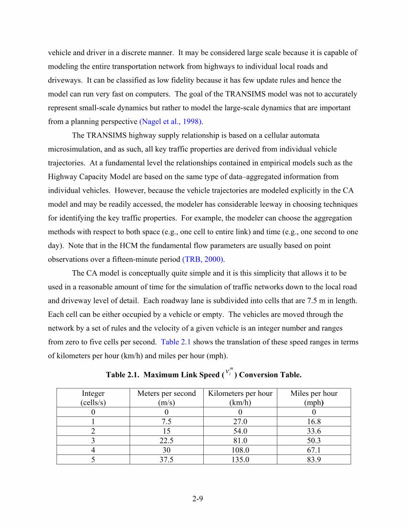
from zero to five cells per second. Table 2.1 shows the translation of these speed ranges in terms

of kilometers per hour (km/h) and miles per hour (mph).

Table 2.1. Maximum Link Speed (miv ) Conversion Table.

Integer (cells/s)

Meters per second (m/s)

Kilometers per hour (km/h)

Miles per hour (mph)

0 0 0 0 1 7.5 27.0 16.8 2 15 54.0 33.6 3 22.5 81.0 50.3 4 30 108.0 67.1 5 37.5 135.0 83.9

2-10

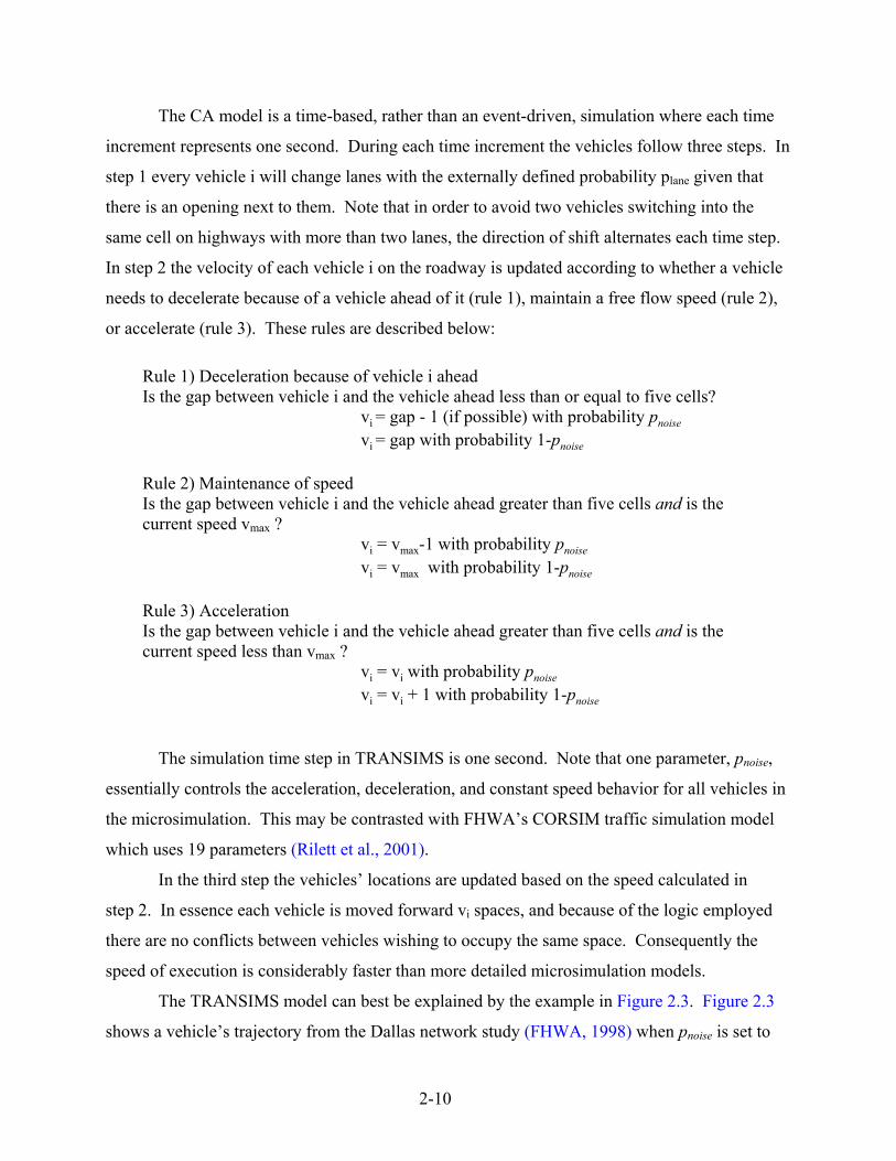
The CA model is a time-based, rather than an event-driven, simulation where each time

increment represents one second. During each time increment the vehicles follow three steps. In

step 1 every vehicle i will change lanes with the externally defined probability plane given that

there is an opening next to them. Note that in order to avoid two vehicles switching into the

same cell on highways with more than two lanes, the direction of shift alternates each time step.

In step 2 the velocity of each vehicle i on the roadway is updated according to whether a vehicle

needs to decelerate because of a vehicle ahead of it (rule 1), maintain a free flow speed (rule 2),

or accelerate (rule 3). These rules are described below:

Rule 1) Deceleration because of vehicle i ahead Is the gap between vehicle i and the vehicle ahead less than or equal to five cells? vi = gap - 1 (if possible) with probability pnoise

vi = gap with probability 1-pnoise

Rule 2) Maintenance of speed Is the gap between vehicle i and the vehicle ahead greater than five cells and is the current speed vmax ? vi = vmax-1 with probability pnoise

vi = vmax with probability 1-pnoise

Rule 3) Acceleration Is the gap between vehicle i and the vehicle ahead greater than five cells and is the current speed less than vmax ? vi = vi with probability pnoise

vi = vi + 1 with probability 1-pnoise

The simulation time step in TRANSIMS is one second. Note that one parameter, pnoise,

essentially controls the acceleration, deceleration, and constant speed behavior for all vehicles in

the microsimulation. This may be contrasted with FHWA’s CORSIM traffic simulation model

which uses 19 parameters (Rilett et al., 2001).

In the third step the vehicles’ locations are updated based on the speed calculated in

step 2. In essence each vehicle is moved forward vi spaces, and because of the logic employed

there are no conflicts between vehicles wishing to occupy the same space. Consequently the

speed of execution is considerably faster than more detailed microsimulation models.

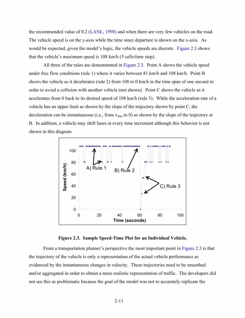
The TRANSIMS model can best be explained by the example in Figure 2.3. Figure 2.3

shows a vehicle’s trajectory from the Dallas network study (FHWA, 1998) when pnoise is set to

2-11

the recommended value of 0.2 (LANL, 1998) and when there are very few vehicles on the road.

The vehicle speed is on the y-axis while the time since departure is shown on the x-axis. As

would be expected, given the model’s logic, the vehicle speeds are discrete. Figure 2.3 shows

that the vehicle’s maximum speed is 108 km/h (5 cells/time step).

All three of the rules are demonstrated in Figure 2.3. Point A shows the vehicle speed

under free flow conditions (rule 1) where it varies between 81 km/h and 108 km/h. Point B

shows the vehicle as it decelerates (rule 2) from 108 to 0 km/h in the time span of one second in

order to avoid a collision with another vehicle (not shown). Point C shows the vehicle as it

accelerates from 0 back to its desired speed of 108 km/h (rule 3). While the acceleration rate of a

vehicle has an upper limit as shown by the slope of the trajectory shown by point C, the

deceleration can be instantaneous (i.e., from vmax to 0) as shown by the slope of the trajectory at

B. In addition, a vehicle may shift lanes at every time increment although this behavior is not

shown in this diagram.

Figure 2.3. Sample Speed-Time Plot for an Individual Vehicle.

From a transportation planner’s perspective the most important point in Figure 2.3 is that

the trajectory of the vehicle is only a representation of the actual vehicle performance as

evidenced by the instantaneous changes in velocity. These trajectories need to be smoothed

and/or aggregated in order to obtain a more realistic representation of traffic. The developers did

not see this as problematic because the goal of the model was not to accurately replicate the

0

20

40

60

80

100

0 20 40 60 80 100Time (seconds)

Spee

d (k

m/h

)

A) Rule 1 B) Rule 2

C) Rule 3

2-12

movement of individual vehicles but rather to model the aggregate traffic behavior (Nagel et al.,

1997). Thus, the model is calibrated to macroscopic traffic measurements, and this is why the

emissions model does not use the individual trajectories from the simulated vehicles as input but

rather data that have been aggregated over space and time (Williams et al., 1999). This point

was made in Figure 2.1 where it was shown that the emissions are calculated in a separate

module rather than being calculated directly within the microsimulation.

2.3.3 Fundamental Properties of TRANSIMS

Typically transportation professionals model the highway supply relationship using a

speed-volume-density function (TRB, 2000). Obviously the TRANSIMS speed-volume-density

relationship cannot be identified a priori based on the CA rules, and therefore must be identified

from the simulation results. In this situation the speed-volume-density and associated link

attributes, such as link capacity, are emergent from the model.

The boundary conditions for link speed are zero and the free flow speed (vf). In most

planning-based supply models the free flow speed would be simply equal to the free flow speed

(or speed limit) as input by the user. In the TRANSIMS model, however, while the user

specifies a maximum speed on a link, this is not equal to the free flow speed. Rather, the free

flow speed is calculated by taking the average value of the speed of vehicles when they are not

impeded by other vehicles. For example, the vehicle in Figure 2.3 is traveling unimpeded from

time zero to 60 seconds, and the output average speed for this vehicle is approximately

105 km/h. This approach to identifying free flow speed corresponds to the definition of free

flow speed in the HCM:

“the average speed of vehicles over a basic freeway segment or a multilane

highway under conditions of low volume, in veh/h (TRB, 2000).”

It is important to note that the free flow speed for a given link can be estimated prior to

the simulation model being run using Equation 2.2 (LANL, 1998).

( ) ( ) noise

minoise

minoise

mi

fi pvpvpvv −=−+−= 11 [2.2]

where: f

iv =

free flow speed on link i (cells/s). Discrete value in range 0-5 cells/s or 0-27 km/h;

2-13

miv = maximum speed on link i (cells/s). Discrete value in range 0-5 cells/s or

0-27 km/h; and pnoise = global calibration parameter related to driving characteristics of population.

Range is approximately 0.0 – 0.3. Default value is 0.2.

Because TRANSIMS is a simulation model the actual output free flow speed on average

will be equal to the value calculated in Equation 2.2 but will, in all likelihood, be slightly

different due to the stochastic nature of the model. In summary, the user sets the link free flow

speed which the model calculates internally using the link variable miv and the global variable

pnoise.

In essence the output from TRANSIMS microsimulation has to be aggregated in order to

obtain link attributes such as free flow speed and other data that are derived from the simulation

such as vehicle emissions. It would be expected based on an examination of Equation 2.2 that as

pnoise increases the free flow speed decreases. However, under certain circumstances the free

flow speed will have a discrete increase when pnoise is increased. The reasons for this

counterintuitive behavior lie in the discrete nature of the CA model. In the TRANSIMS model

the speed limit on each link is input in terms of km/h. This input value is subsequently converted

to a step/second speed, and it is unlikely that the input speed will translate into one of the

acceptable integer values shown in Table 2.1. Therefore, Equation 2.3, which was identified

directly from the TRANSIMS code, is used to transition between the input speed value and the

value that is actually used.

L

round =

+ noise

sim

i pv

v [2.3]

where: siv = input speed on link i (m/s). (This is referred to as speed limit of link in the

TRANSIMS user manual); and L = length of cell in m/cell (7.5 m by definition).

The round function in Equation 2.3 rounds the real number down if the value to the right

of the decimal point is less than 0.5 and up if is equal to or greater than 0.5. The maximum

speed on a link is a function of the input speed limit, the fixed cell length value, and the input

value of pnoise. In essence, TRANSIMS attempts to find the integer value of miv which makes

fiv ,

as defined in Equation 2.2, as close as possible to the input speed limit. Equations 2.2 and 2.3

2-14

show that while in general miv decreases as pnoise increases, at certain locations the value for

miv can have a large and discrete increase with a small increase in pnoise. Figure 2.4 illustrates the

relationship between input speed limit and the free flow speed where the y-axis represents the

free flow speed, the x-axis represents the value of pnoise, and the numbers on the graph indicate

the input speed limit. When the link speed is input as 100 km/h the estimated free flow speed

will be approximately 108 km/h, 100 km/h, and 94.5 km/h when pnoise is 0.0, 0.29, and 0.5,

respectively. This may be contrasted to an input free flow speed of 90 km/h which ranges from

81 km/h to 76.5 km/h for pnoise values of 0.0 to 0.166, respectively, and then has the same values

as that of a 100 km/h input free flow speed for pnoise values greater than 0.166. Interestingly, the

microsimulation model can only model a link speed of 90 km/h, when the input speed limit is 90

km/h, if the pnoise value is 0.665. There is no difference in free flow speeds that have input link

speeds of 70 km/h and 80 km/h. Therefore, it would be impossible to analyze the effect on link

properties, such as the amount of air pollution associated with a link, when the link speed limit is

decreased from 80 km/h to 70 km/h because the model would not be able to differentiate

between the two situations. Clearly, the TRANSIMS model has an implicit accuracy level which

transportation planners will need to understand before they can analyze the simulation results.

Figure 2.4. Free Flow Speed versus Parameter pnoise.

For transportation planners the important point to realize is that the nature of the

TRANSIMS CA model means that they will have to undergo a fundamental change in how they

think about supply relationships in their analyses. In order to model a fundamental property such

0

20

40

60

80

100

120

140

0 0.1 0.2 0.3 0.4 0.5 0.6pnoise

Free

Flow

Spee

d(k

m/h

) 120 km/h100 km/h

90 km/h70 and 80 km/h

60 km/h

2-15

as free flow speed they will have to choose an appropriate value of pnoise and miv . One of the

advantages to TRANSIMS is that the modeling system is modular and transparent. Therefore, it

is relatively easy to change the source code to avoid some of the counterintuitive behavior shown

above or even to substitute a different microsimulation model. In summary transportation

planners will have to keep a number of points in mind when using this new generation of models.

In particular, 1) some of the boundary conditions are not emergent and will need to be estimated

ahead of time; 2) because of the nature of the model small changes in calibration parameters,

such as pnoise, may have relatively large effects on traffic parameters such as free flow speed; 3) it

is a discrete model so at the individual vehicle profile level rounding will occur; 4) only the

aggregated traffic flow output has been calibrated; and 5) it is extremely important for the

modelers to have a good understanding of the logic of the model and its implications on results.

The boundary conditions for the density on a given link i will be 0 and the jam density

( jiρ ). The HCM defines jam density as “the density at which congestion becomes so severe that

all movements of persons or vehicles stop, usually expressed as vehicles per km per lane” (TRB,

2000). Because of the discrete nature of the model, jiρ is effectively equal to the situation when

all of the cells are filled. Given that the cell size is 7.5 m, jam density is equivalent to one

vehicle per 7.5 m per lane or 133 vehicles per km per lane (LANL, 1998).

The boundary conditions for volume are dependent on the boundary conditions for

density and speed. At the boundary conditions of zero speed and free flow speed (or 0 density

and jam density) the link volume is zero.

The speed-density-volume relationship is emergent from the model once the boundary

conditions are set. One of the most important link parameters used by transportation planners in

analyzing a network is link capacity. As discussed above, in most planning models capacity is

deterministic and identified exogenous to the model as was shown in Equation 2.1. While the

TRANSIMS model includes a capacity attribute in the input field, it is not used within the

program. Instead the value of capacity is emergent from the model.

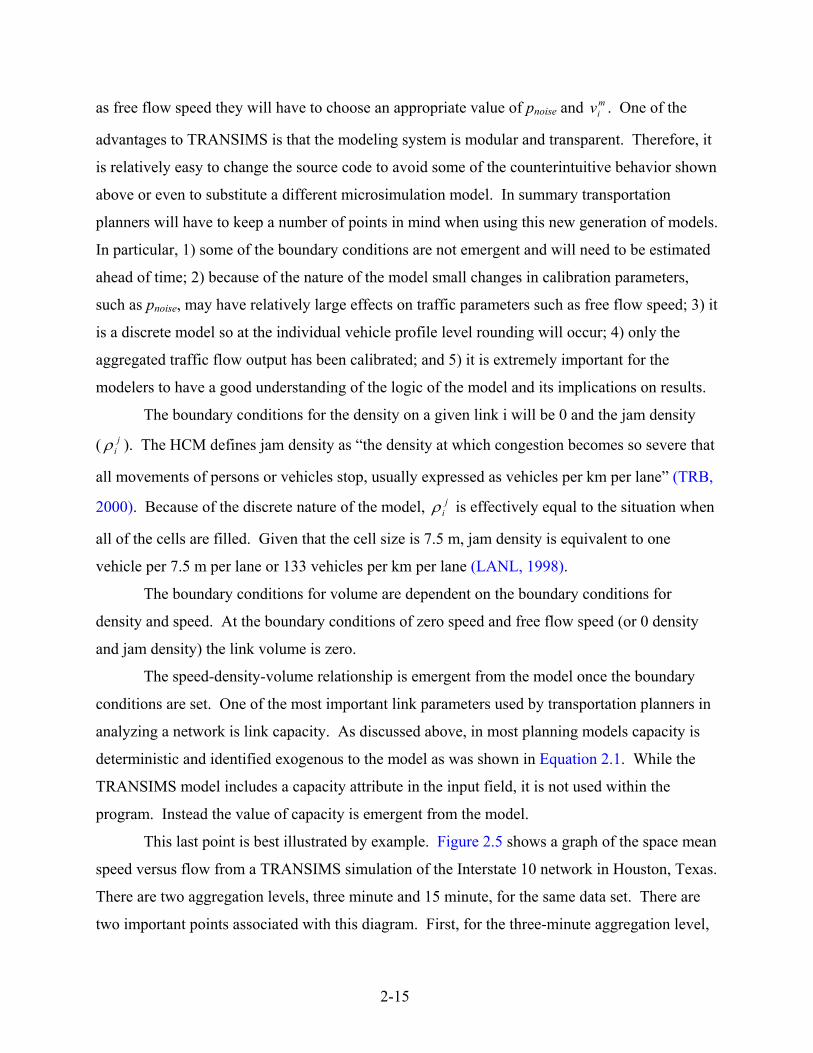
This last point is best illustrated by example. Figure 2.5 shows a graph of the space mean

speed versus flow from a TRANSIMS simulation of the Interstate 10 network in Houston, Texas.

There are two aggregation levels, three minute and 15 minute, for the same data set. There are

two important points associated with this diagram. First, for the three-minute aggregation level,

2-16

which is the value used in the LANL calibrations, the capacity is approximately 2050 veh/h/lane.

The speed-flow diagram may be contrasted with traditional planning supply models, such as the

0

20

40

60

80

100

120

0 500 1000 1500 2000

Flow (veh/h per lane)

Spee

d (k

m/h

)

3 minute15 minute

Aggregation Level

Figure 2.5. Speed versus Flow for Different Aggregation Intervals for I-10 Corridor in

Houston, Texas.

Bureau of Public Roads function, where volumes greater than capacity are allowed (U.S.

Department of Commerce, 1964). The second point is that this capacity value was never input

into the model – rather it was identified (or emerged) from the microsimulation. However,

because capacity is emergent, transportation planners will have to be more knowledgeable about

traffic engineering concepts. For example, capacity is defined with respect to a specific time

period and therefore different temporal aggregation periods will result in different estimates of

capacity for the same input data. Figure 2.6 shows that the capacity for the 15-minute

aggregation level, which is the time period used in the HCM, is approximately 1700 veh/h/lane.

This is not unexpected, as the measured capacity tends to decrease as observation times increase.

It is proposed in this report that the HCM definition of 15 minutes be adopted uniformly by the

TxDOT transportation planning group so that 1) the definition is consistent with traffic

operations definitions, and 2) results can be compared readily across different planning agencies

with input from traffic operations groups.

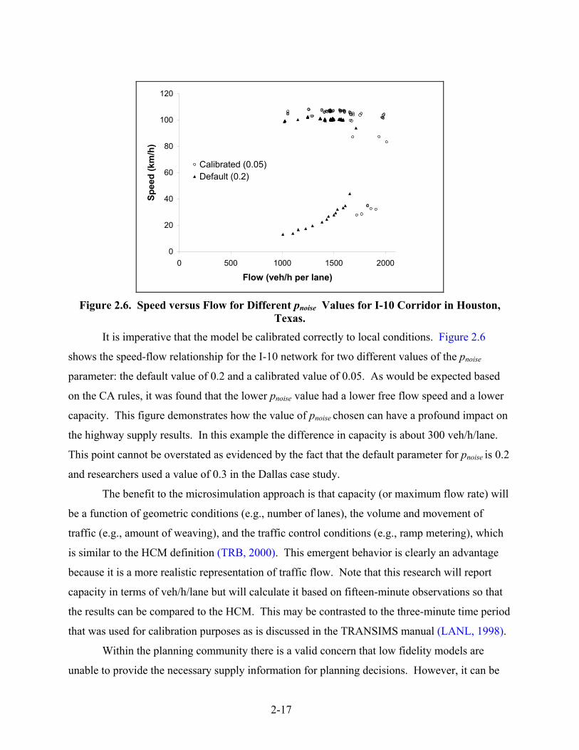
2-17

0

20

40

60

80

100

120

0 500 1000 1500 2000

Flow (veh/h per lane)

Spee

d (k

m/h

)Calibrated (0.05)Default (0.2)

Figure 2.6. Speed versus Flow for Different pnoise Values for I-10 Corridor in Houston,

Texas.

It is imperative that the model be calibrated correctly to local conditions. Figure 2.6

shows the speed-flow relationship for the I-10 network for two different values of the pnoise

parameter: the default value of 0.2 and a calibrated value of 0.05. As would be expected based

on the CA rules, it was found that the lower pnoise value had a lower free flow speed and a lower

capacity. This figure demonstrates how the value of pnoise chosen can have a profound impact on

the highway supply results. In this example the difference in capacity is about 300 veh/h/lane.

This point cannot be overstated as evidenced by the fact that the default parameter for pnoise is 0.2

and researchers used a value of 0.3 in the Dallas case study.

The benefit to the microsimulation approach is that capacity (or maximum flow rate) will

be a function of geometric conditions (e.g., number of lanes), the volume and movement of

traffic (e.g., amount of weaving), and the traffic control conditions (e.g., ramp metering), which

is similar to the HCM definition (TRB, 2000). This emergent behavior is clearly an advantage

because it is a more realistic representation of traffic flow. Note that this research will report

capacity in terms of veh/h/lane but will calculate it based on fifteen-minute observations so that

the results can be compared to the HCM. This may be contrasted to the three-minute time period

that was used for calibration purposes as is discussed in the TRANSIMS manual (LANL, 1998).

Within the planning community there is a valid concern that low fidelity models are

unable to provide the necessary supply information for planning decisions. However, it can be

2-18

argued that even simple microsimulation models are vastly superior to macroscopic models, such

as the BPR equation, which cannot model realistically oversaturated roadway conditions. Tests

on two freeway networks in Houston indicated that TRANSIMS, using calibrated parameters,

could replicate observed volumes to within 10 percent during congested conditions and within

1 percent during uncongested conditions (Rilett et al., 2000). More importantly, a similar

analysis using the high fidelity CORSIM traffic operations model found comparable error rates

with respect to estimated speeds and travel times. Therefore, while further study on different

freeways and operating conditions is necessary, the preliminary results indicate that TRANSIMS

is as accurate as the state of the practice (high fidelity traffic operations models with respect to

modeling freeway sections).

2.3.4 Modeling Interrupted Flow Facilities

Modeling interrupted flow conditions, such as roadways with signalized intersections, is

inherently more complex than modeling uninterrupted flow conditions such as freeways.

Because interrupted flow conditions are a function of more variables, the number of CA

operating rules was increased for vehicles at traffic signals (LANL, 1993). When a vehicle

approaches an intersection it is forced to queue if it does not have permission to proceed (i.e.,

traffic signal is red) or if it is unable to initiate its maneuver (i.e., when the gap in the conflicting

traffic stream is too small). If it is allowed to enter the intersection it is placed in a queue buffer

for the duration of its movement in the intersection. The duration consists of the input parameter

dwell time (i.e., time it takes to make the movement) plus any delay time due to conflicts with

other vehicles. For example, if the vehicle cannot enter the downstream link because of the

presence of another vehicle, it will “stay” in the intersection until the other vehicle has moved

downstream. Note that once a vehicle enters the intersection, such issues as conflicts, size

constraints, and similar factors are not examined. Full details of the CA logic for intersections

can be found elsewhere (Nagel et al., 1997).

In order to study the traffic signal logic, TRANSIMS was calibrated to the observed

volume and control delay at a diamond interchange in College Station, Texas (Rilett and Kim,

2001). The calibrated pnoise parameter was 0.3 and the calibrated dwell time parameter was five

seconds which may be contrasted to the default values of 0.2 and two seconds, respectively. As

discussed previously, the highway calibrations identified pnoise to be 0.1. Because pnoise is a

global parameter it is hypothesized that the different calibration values found in the highway and

2-19

diamond interchange analyses could be problematic when networks that have both urban

freeways and traffic signals have to be calibrated. A logical solution might be to allow pnoise to

vary by the type of link although the method for implementing this concept would need further

study.

The TRANSIMS results were compared to results from the Texas Transportation

Institute’s (TTI) macroscopic traffic signal optimization package, PASSER III, and results from

the microsimulation traffic operations analysis model CORSIM. For the observed conditions

PASSER III, CORSIM and TRANSIMS all were able to represent adequately the demand within

1 percent and to estimate the control delay to within 5 percent. The fact that the TRANSIMS

traffic signal logic had the same error range as the high fidelity CORSIM model and the

macroscopic PASSER III model gives credence to the basic low fidelity approach.

Researchers conducted a series of sensitivity analyses to test the conditions under which

TRANSIMS, CORSIM, and PASSER III gave similar results. The variables examined were the

type of phase sequence, the offset, the cycle length, the traffic demand, and the signal spacing.

CORSIM tended to follow similar patterns to PASSER III for all of the analyses. In addition, all

three models predict similar control delay values as a function of cycle. Similar results were

found when sensitivity analyses were performed on offset, traffic demand, and signal spacing.

TRANSIMS was less sensitive, however, to the latter variables as compared to CORSIM. In

addition, it was found that phase sequence had no effect on the simulated results.

2.3.5 Analysis of Output

One of the main advantages of the microsimulation approach is that there are

significantly more options when it comes to analyzing data output. Because each simulated

traveler is tracked individually, the user has the option of choosing any level of disaggregation

for analyzing the data. For example, the information can be output by type of trip, by trip

location, by traveler characteristics, or by other factors depending on the needs of the end

decision maker. In addition, because of the stochastic nature of the model, not only the means

but also the standard errors of all estimated values can be derived. Therefore, it is considerably

easier to develop and calculate meaningful measures of effectiveness as compared to the output

from the four-step process.

The potential of TRANSIMS to provide customized data for analysis was shown in an

ITS automatic data collection study. In particular, TRANSIMS was used to compare and

2-20

contrast the output from automatic vehicle identification (AVI) and inductance loop ITS data

collection systems for vehicle emissions analysis (Zietsman and Rilett, 2001). It was shown that

loop detector data could result in relatively large under-estimations of vehicular emissions

whereas AVI data produced results that were close to those obtained based on complete

knowledge of the movement of the vehicles. Because similarly accurate results were obtained

from CORSIM, this study illustrates the point that low fidelity microscopic models such as

TRANSIMS can be used to analyze ITS technologies—something that cannot be done

adequately with the macroscopic four-step model.

In addition, information can be identified on the entire network or on specific

components of it, such as specific links or corridors. The ability to choose the output format has

proven invaluable when calibrating the model to both inductance loop and automatic vehicle

identification data (Rilett et al., 2000). As an example, the output data may be manipulated to

match that from real time ITS data collection systems. Figure 2.7a illustrates a contour plot of

speed profiles along the North Central Expressway corridor in Dallas, Texas. The x-axis

represents distance while the y-axis represents time of day. Light gray represents uncongested

conditions (>80 km/h) and dark gray represents congested conditions (<20 km/h). Figure 2.7a

shows that the speeds are relatively high except for some severe congestion at approximately the

13 km point which begins at approximately 8:00 a.m. and lasts until approximately 10:00 a.m.

This congestion begins to spill upstream at approximately 9:00 a.m. Because ITS information,

such as spot speeds from inductance loops, often are displayed as contour plots, a comparison

between the simulated and real data can be accomplished easily. In addition, the ability to access

realistic simulation data and to display it in contour plot format will allow planners to identify

where bottlenecks are likely to occur in the future as demand, geometric alignment, and so on

change. Lastly, Figure 2.7b shows a contour plot from the same corridor where it is clear that

the speeds are fairly uniform and the corridor is mildly congested. Note that the only difference

between the two graphs is that the results in Figure 2.7a were based on the default pnoise value of

0.2 while the results from Figure 2.7b were based on the pnoise value of 0.3 that was used in the

2-21

9 8 . 7 8 0 5 9 8 . 8 4 9 4 9 9 . 6 1 1 7 9 5 . 8 5 8 0 9 9 . 0 0 0 0 8 7 . 7 5 0 0 1 0 3 . 2 3 5 3 9 9 . 2 4 3 2 9 8 . 7 4 2 9 9 8 . 6 0 8 7 9 3 . 4 4 6 8 9 8 . 3 5 7 1 9 8 . 3 5 7 11 0 0 . 1 1 2 4 9 9 . 2 1 2 6 9 9 . 0 6 2 1 9 3 . 1 0 3 4 8 4 . 8 5 7 1 9 1 . 0 0 0 0 9 6 . 4 2 8 6 9 8 . 5 7 7 2 9 8 . 7 4 2 9 1 0 0 . 2 8 5 7 9 6 . 2 7 5 6 1 0 0 . 5 1 0 9 9 9 . 2 4 3 2

9 9 . 3 1 0 3 9 9 . 4 3 1 8 9 8 . 5 7 4 9 9 4 . 8 0 9 2 1 0 2 . 8 0 7 7 9 3 . 1 2 2 4 9 5 . 6 2 5 0 1 0 0 . 0 9 6 3 9 9 . 9 6 6 9 9 9 . 9 4 8 6 9 4 . 1 1 4 3 9 9 . 7 8 2 6 9 9 . 2 4 3 29 9 . 5 9 0 2 9 9 . 2 9 9 5 9 8 . 6 5 3 8 9 7 . 3 3 9 1 9 9 . 0 0 0 0 9 3 . 0 3 6 1 9 9 . 7 8 2 6 9 9 . 2 6 4 0 1 0 0 . 1 7 3 9 9 9 . 4 2 8 6 9 6 . 3 7 6 2 9 9 . 3 8 9 8 9 8 . 0 3 8 8

1 0 0 . 0 0 0 0 9 8 . 5 1 6 4 9 8 . 2 1 8 0 9 6 . 4 7 6 4 1 0 0 . 6 7 8 0 9 5 . 4 1 7 5 1 0 6 . 0 7 1 4 9 8 . 6 6 6 2 1 0 1 . 1 0 6 4 9 8 . 3 8 7 4 9 3 . 9 3 5 4 9 9 . 7 8 2 6 9 7 . 5 6 5 21 0 1 . 2 5 0 0 9 7 . 6 9 7 4 9 8 . 6 5 3 8 9 7 . 5 0 0 0 9 5 . 8 0 6 5 8 6 . 8 4 5 4 1 0 5 . 8 8 2 4 9 7 . 3 7 4 3 1 0 0 . 3 3 5 5 9 9 . 9 1 1 9 9 3 . 3 7 3 2 9 9 . 4 7 3 7 1 0 0 . 0 1 5 6

9 9 . 3 6 0 0 9 8 . 8 9 5 3 9 8 . 7 1 7 1 9 9 . 8 1 0 4 1 0 0 . 3 3 7 8 8 8 . 8 6 0 8 9 6 . 8 4 7 8 9 9 . 3 8 1 0 1 0 0 . 2 3 2 0 1 0 1 . 3 9 5 7 9 4 . 8 1 6 6 1 0 0 . 5 1 0 9 9 9 . 9 1 8 49 7 . 7 9 5 3 9 7 . 9 1 1 1 9 9 . 1 4 8 2 9 7 . 5 9 0 4 1 0 0 . 8 6 7 9 8 9 . 8 5 6 0 9 7 . 7 5 8 6 9 8 . 4 6 3 7 9 9 . 2 6 8 1 9 8 . 8 4 7 5 9 1 . 6 1 8 4 9 9 . 3 8 9 8 1 0 2 . 0 0 0 09 9 . 7 4 5 2 9 8 . 4 3 7 5 9 8 . 7 4 8 8 9 6 . 0 7 9 1 9 6 . 7 7 5 3 8 9 . 7 5 3 4 9 8 . 7 8 0 5 9 5 . 7 4 4 5 9 9 . 2 8 3 2 9 8 . 9 4 0 6 9 4 . 7 7 8 5 1 0 0 . 0 0 0 0 9 9 . 5 1 2 29 8 . 7 0 2 0 9 7 . 9 9 2 1 9 8 . 1 9 2 3 9 7 . 9 8 3 9 1 0 0 . 2 8 5 7 8 8 . 1 6 5 9 9 3 . 3 8 3 5 9 7 . 8 5 2 3 1 0 0 . 2 1 3 2 9 8 . 6 8 0 2 9 3 . 9 7 7 8 9 9 . 1 9 4 5 9 8 . 7 0 9 79 9 . 1 4 5 5 9 7 . 9 3 4 8 9 8 . 8 7 5 7 9 8 . 0 6 3 0 9 5 . 5 3 8 5 9 0 . 1 4 0 1 1 0 2 . 1 0 0 8 9 6 . 6 9 8 1 9 9 . 6 4 5 6 9 8 . 3 1 0 0 9 3 . 3 3 4 8 1 0 0 . 1 7 8 6 1 0 0 . 0 0 0 09 9 . 8 1 0 4 9 7 . 9 4 2 8 9 8 . 6 3 4 1 9 6 . 6 9 7 7 9 3 . 2 6 0 9 8 4 . 3 7 5 0 9 9 . 2 0 9 3 9 3 . 5 0 4 2 9 9 . 6 9 2 3 9 6 . 6 0 3 7 9 3 . 3 4 7 5 9 9 . 3 1 9 9 9 8 . 6 7 7 59 9 . 2 9 0 3 9 7 . 5 3 0 1 9 8 . 1 6 3 0 9 7 . 5 1 6 9 9 4 . 3 7 3 8 8 1 . 6 1 1 1 9 4 . 5 0 0 0 9 3 . 4 6 1 5 9 9 . 7 1 8 6 9 6 . 1 9 2 3 9 2 . 4 1 1 6 1 0 0 . 5 6 7 4 9 9 . 4 9 9 49 9 . 8 7 3 1 9 7 . 8 3 4 4 9 8 . 8 4 3 9 9 7 . 7 0 9 8 9 3 . 2 9 8 4 7 7 . 0 6 5 9 9 0 . 0 0 0 0 8 7 . 3 3 5 1 1 0 0 . 2 4 6 6 9 1 . 5 7 3 7 8 9 . 9 4 1 2 9 9 . 4 1 2 1 9 9 . 4 3 9 9

1 0 0 . 0 0 0 0 9 8 . 1 2 9 7 9 8 . 7 0 1 3 9 6 . 7 1 6 4 8 9 . 5 9 7 8 8 0 . 4 2 3 3 8 6 . 5 7 1 4 8 9 . 4 3 4 5 9 9 . 2 2 8 9 9 3 . 5 4 7 2 8 8 . 2 3 9 4 1 0 0 . 7 2 1 0 9 9 . 0 7 2 31 0 0 . 5 0 6 1 9 8 . 5 3 7 2 9 7 . 0 5 9 1 9 6 . 0 6 8 2 9 2 . 3 3 1 6 8 0 . 1 7 0 8 9 1 . 2 5 4 4 9 1 . 9 0 1 5 9 9 . 3 2 7 1 9 4 . 5 0 0 0 9 2 . 9 4 5 8 9 9 . 9 9 4 7 9 9 . 0 8 5 7

9 8 . 6 9 5 4 9 7 . 8 4 2 2 9 7 . 6 3 7 5 9 4 . 1 8 6 0 9 4 . 9 1 7 5 8 2 . 4 6 8 0 9 6 . 3 6 0 4 9 1 . 8 4 8 9 9 9 . 9 0 5 8 9 5 . 0 5 9 0 9 2 . 1 1 6 9 1 0 0 . 2 7 8 1 1 0 0 . 4 2 3 31 0 0 . 2 8 5 7 9 7 . 2 9 3 7 9 7 . 6 5 1 2 9 5 . 3 5 7 1 9 7 . 2 4 7 8 7 7 . 8 7 4 6 8 8 . 7 1 4 3 8 4 . 1 2 1 9 9 9 . 5 7 1 1 9 2 . 6 1 3 0 8 9 . 5 4 1 0 9 9 . 2 5 6 3 1 0 1 . 1 0 1 3

9 8 . 5 7 8 4 9 6 . 9 1 3 2 9 8 . 1 3 6 6 9 6 . 7 0 3 2 9 4 . 6 9 5 7 7 8 . 9 3 5 5 7 6 . 3 5 7 5 4 9 . 4 7 3 1 9 7 . 0 7 8 7 9 7 . 2 0 0 0 9 2 . 8 8 7 5 9 9 . 4 7 3 7 9 9 . 0 4 5 09 8 . 8 7 0 1 9 5 . 2 4 0 8 9 6 . 0 6 0 7 9 7 . 0 1 1 6 9 3 . 2 1 9 0 7 5 . 7 0 5 9 8 1 . 0 0 0 0 3 2 . 4 5 0 5 9 8 . 6 2 0 3 9 3 . 5 4 6 9 9 1 . 1 3 8 3 9 9 . 7 0 6 6 9 9 . 9 0 8 59 7 . 8 2 4 4 9 6 . 2 9 1 5 9 7 . 4 2 7 1 9 8 . 4 6 2 3 9 2 . 7 5 9 3 7 8 . 3 1 0 8 9 7 . 0 5 4 1 2 5 . 7 5 4 1 9 8 . 5 2 6 3 9 5 . 5 1 6 7 9 1 . 7 4 8 6 1 0 0 . 0 7 2 7 1 0 0 . 1 4 5 59 7 . 3 3 9 1 9 3 . 9 1 6 4 9 6 . 5 1 5 3 9 7 . 7 7 1 6 8 8 . 2 9 7 3 7 9 . 6 3 4 4 9 9 . 8 0 2 0 2 8 . 0 8 8 9 9 7 . 2 1 2 4 9 5 . 0 9 5 4 9 0 . 5 1 6 1 9 9 . 7 8 2 6 9 9 . 2 9 2 09 7 . 6 0 2 2 9 0 . 4 9 7 9 9 5 . 1 2 6 9 9 7 . 6 2 7 1 8 7 . 2 8 1 6 8 4 . 2 2 3 4 8 7 . 4 4 3 2 3 0 . 4 5 6 4 9 8 . 6 2 0 3 9 7 . 5 9 7 6 9 4 . 0 0 2 4 9 9 . 8 6 0 1 9 9 . 9 4 9 79 8 . 8 0 8 5 8 9 . 8 4 3 0 9 4 . 5 6 7 9 9 6 . 9 7 6 2 8 5 . 3 0 8 5 7 9 . 9 8 9 8 8 7 . 9 4 6 1 1 9 . 6 3 8 4 9 8 . 3 4 1 5 9 7 . 3 1 3 2 8 9 . 5 1 4 2 9 9 . 6 0 9 4 9 9 . 7 4 2 59 4 . 6 6 0 3 8 8 . 7 5 4 2 9 3 . 5 2 7 5 9 7 . 9 8 1 8 8 1 . 3 6 3 8 7 9 . 6 8 1 0 9 3 . 8 2 9 8 1 7 . 9 3 8 1 9 6 . 9 5 3 3 9 2 . 0 7 1 2 5 6 . 7 9 3 1 9 9 . 9 8 3 2 9 9 . 9 8 6 49 5 . 9 4 8 8 8 2 . 4 8 6 5 9 2 . 3 6 6 1 9 5 . 7 9 7 8 8 6 . 0 0 3 9 8 3 . 2 5 8 4 9 4 . 7 5 9 6 1 6 . 5 7 2 1 9 8 . 0 9 9 2 9 2 . 9 2 9 5 5 0 . 8 8 3 7 9 9 . 8 8 2 4 9 9 . 6 5 1 39 3 . 8 8 0 9 8 6 . 5 7 5 1 9 4 . 3 5 9 5 9 8 . 0 7 4 0 8 1 . 6 0 3 8 8 1 . 2 8 8 2 9 8 . 7 3 5 9 2 0 . 2 6 8 4 9 7 . 3 8 4 0 9 4 . 7 0 9 1 4 8 . 3 2 5 9 9 9 . 0 5 0 5 9 9 . 9 6 6 99 4 . 7 8 0 1 7 8 . 9 3 9 6 9 1 . 8 0 4 5 9 6 . 7 0 1 5 7 5 . 5 0 8 5 8 1 . 0 5 7 2 9 4 . 8 0 4 9 2 5 . 5 6 8 7 9 9 . 1 8 4 8 9 5 . 9 5 6 1 4 0 . 3 2 7 2 1 0 0 . 6 2 1 6 1 0 0 . 5 3 7 29 4 . 0 2 5 0 6 9 . 9 0 8 4 7 8 . 7 1 2 1 9 8 . 3 9 3 8 7 6 . 7 0 8 6 8 2 . 7 1 0 9 9 7 . 6 8 2 9 2 6 . 2 3 1 0 9 6 . 6 3 7 9 9 5 . 0 0 2 2 3 7 . 3 7 4 4 9 9 . 6 6 8 6 1 0 0 . 0 6 6 49 5 . 3 7 3 1 6 4 . 4 8 6 7 6 1 . 7 5 6 0 9 6 . 3 6 4 2 8 3 . 2 3 5 7 8 4 . 0 2 1 8 9 5 . 3 8 3 2 3 2 . 4 6 9 1 9 6 . 6 6 5 3 9 5 . 4 9 2 5 4 5 . 5 1 0 4 9 9 . 6 0 2 2 1 0 0 . 5 2 7 69 5 . 0 2 0 5 6 7 . 6 1 6 4 4 8 . 5 5 2 6 9 6 . 1 2 5 7 8 6 . 5 2 3 7 8 1 . 6 0 4 1 8 7 . 9 8 7 2 3 1 . 2 1 7 3 9 8 . 9 9 4 9 9 2 . 6 7 3 3 3 6 . 4 1 3 5 9 9 . 6 2 6 0 1 0 0 . 0 4 5 59 5 . 3 7 9 1 7 2 . 8 5 0 5 3 8 . 3 4 0 0 9 3 . 7 8 4 6 8 4 . 2 8 3 8 8 5 . 4 7 6 7 9 6 . 5 9 2 8 2 1 . 1 1 5 1 9 9 . 2 8 2 1 9 6 . 2 0 2 8 4 3 . 8 2 8 9 9 9 . 5 2 8 1 9 9 . 4 0 4 08 9 . 0 5 5 2 8 7 . 1 4 6 4 3 7 . 8 3 0 2 9 6 . 5 5 6 3 9 1 . 8 6 6 4 8 4 . 9 6 7 2 9 8 . 0 9 3 5 1 8 . 9 6 8 8 9 8 . 5 2 6 3 9 4 . 4 2 6 2 3 3 . 6 4 1 5 9 9 . 2 1 0 4 9 9 . 9 8 9 69 2 . 1 7 1 8 7 4 . 2 2 0 5 4 7 . 9 9 9 0 9 7 . 4 5 0 9 9 0 . 2 2 7 8 5 5 . 5 5 4 0 1 8 . 8 6 9 9 1 0 . 3 8 9 2 9 8 . 1 0 2 2 9 0 . 7 6 8 4 4 2 . 8 6 1 1 9 9 . 3 7 1 1 9 9 . 8 3 7 89 2 . 0 2 7 1 7 0 . 9 0 1 8 4 3 . 9 5 7 4 9 6 . 7 0 9 2 7 8 . 0 2 1 8 2 5 . 9 6 8 2 1 1 . 1 0 2 0 1 4 . 6 0 9 4 9 9 . 5 7 6 8 9 6 . 4 1 2 3 4 2 . 8 7 7 1 9 9 . 7 4 6 5 9 9 . 6 8 8 89 5 . 5 5 0 7 6 8 . 7 5 4 5 4 4 . 4 3 7 1 9 7 . 5 1 0 9 2 8 . 5 4 8 8 2 1 . 3 9 6 1 1 3 . 5 7 9 9 9 . 7 4 4 3 9 7 . 8 3 9 7 9 4 . 7 1 9 3 4 3 . 8 1 7 9 9 7 . 8 2 7 6 9 9 . 8 0 9 49 3 . 1 5 6 8 8 4 . 8 8 0 2 4 7 . 0 7 8 5 8 1 . 3 8 0 4 1 8 . 6 6 1 9 1 3 . 8 3 6 2 8 . 3 2 4 5 1 0 . 0 2 7 2 9 7 . 2 7 1 5 9 4 . 5 7 3 0 3 7 . 2 3 8 1 9 7 . 6 0 3 4 9 9 . 7 7 5 58 6 . 1 3 6 9 7 2 . 4 7 9 6 4 4 . 8 0 3 5 6 9 . 4 0 2 5 1 4 . 2 3 0 2 1 1 . 7 8 8 1 7 . 0 5 0 2 9 . 6 5 3 2 9 7 . 8 8 9 6 9 6 . 2 0 7 9 3 6 . 3 0 9 8 9 9 . 1 1 9 6 9 9 . 0 8 2 39 4 . 0 4 5 6 8 3 . 1 4 0 9 5 0 . 7 2 4 2 5 2 . 0 8 6 1 5 . 6 6 3 9 7 . 7 7 6 6 5 . 9 2 9 4 9 . 5 8 8 4 9 7 . 6 4 1 0 9 4 . 4 4 7 5 3 1 . 7 3 0 5 9 8 . 8 7 6 0 9 8 . 8 4 1 79 3 . 5 4 2 3 7 4 . 6 4 6 5 4 6 . 9 4 3 0 9 1 . 4 6 6 8 2 0 . 8 2 3 7 1 5 . 9 3 4 7 1 3 . 0 1 8 1 1 2 . 4 6 4 1 9 8 . 4 7 3 7 9 7 . 0 4 9 3 2 4 . 1 7 7 0 9 9 . 7 4 2 5 9 9 . 6 1 4 69 2 . 0 6 0 8 7 5 . 8 6 5 7 4 4 . 7 8 0 9 9 5 . 7 5 2 3 6 0 . 3 2 8 1 1 9 . 9 2 3 3 9 . 4 9 4 0 1 0 . 1 2 4 4 9 9 . 2 9 8 6 9 4 . 6 4 3 9 3 9 . 9 2 5 9 9 9 . 2 0 1 4 1 0 0 . 3 8 8 89 2 . 0 5 9 0 8 0 . 0 8 4 7 4 8 . 8 5 7 1 9 5 . 9 4 9 0 4 5 . 3 5 4 7 1 4 . 1 2 6 0 9 . 0 0 3 7 8 . 6 6 8 3 9 7 . 4 6 9 2 9 4 . 8 5 8 9 5 1 . 1 1 2 6 9 8 . 7 3 2 6 9 9 . 2 6 1 59 5 . 5 0 6 1 9 0 . 7 8 7 2 5 9 . 6 2 6 8 9 8 . 1 2 7 1 3 6 . 1 7 0 2 2 1 . 6 3 4 3 9 . 0 9 1 5 1 0 . 8 2 1 6 9 8 . 1 7 1 0 9 7 . 9 2 0 0 3 7 . 7 3 0 2 9 8 . 1 5 5 4 9 9 . 3 8 0 59 3 . 2 8 2 9 8 8 . 0 4 8 9 8 8 . 8 5 4 5 9 8 . 4 1 9 1 9 0 . 6 8 7 0 2 5 . 5 9 6 1 1 0 . 6 0 0 6 9 . 7 2 8 5 9 8 . 4 2 0 2 9 5 . 6 6 3 6 4 5 . 9 2 7 0 9 8 . 1 6 4 7 1 0 0 . 2 2 6 79 0 . 8 6 3 2 8 0 . 7 2 2 4 9 0 . 9 5 8 7 9 8 . 0 6 6 9 8 0 . 7 7 6 1 2 3 . 1 2 2 8 6 . 8 2 9 3 9 . 0 4 5 1 9 7 . 4 4 3 6 9 7 . 6 7 4 8 4 5 . 1 7 9 9 9 8 . 2 1 3 5 9 9 . 2 5 9 39 2 . 2 5 9 9 8 7 . 1 0 9 5 7 9 . 4 8 6 7 9 7 . 4 7 5 5 8 2 . 3 6 5 4 2 7 . 3 7 7 3 9 . 8 1 0 6 9 . 7 5 6 9 9 7 . 9 4 7 0 9 7 . 3 9 4 8 4 7 . 6 3 4 7 9 9 . 0 3 7 3 9 8 . 1 4 9 29 4 . 8 1 0 2 8 2 . 0 1 5 7 5 2 . 3 4 9 3 9 2 . 4 5 9 8 8 2 . 8 6 0 5 6 8 . 6 2 1 1 2 2 . 1 1 8 3 1 0 . 7 7 1 3 9 7 . 6 2 7 1 9 8 . 6 3 8 5 1 7 . 0 8 7 7 9 8 . 5 1 4 8 9 8 . 6 6 4 99 2 . 9 4 3 7 8 0 . 1 7 6 6 4 1 . 0 3 7 6 7 5 . 7 3 6 5 9 0 . 4 1 8 6 8 6 . 7 1 2 2 9 9 . 0 4 8 9 8 . 6 3 6 0 9 8 . 9 0 5 9 9 7 . 2 0 0 0 3 4 . 2 5 7 6 9 9 . 2 3 5 2 9 9 . 3 0 9 59 4 . 9 7 2 4 8 8 . 4 0 6 7 7 5 . 3 0 5 3 3 1 . 2 6 9 7 8 4 . 1 1 5 4 8 4 . 6 4 6 3 9 8 . 8 0 8 5 9 . 6 9 6 1 9 8 . 4 1 3 5 9 7 . 0 4 4 5 2 5 . 6 2 0 5 9 9 . 1 6 6 7 9 9 . 5 8 3 99 6 . 6 9 2 8 9 1 . 2 9 2 0 9 5 . 0 0 7 9 9 7 . 7 1 8 5 9 0 . 3 3 1 8 7 9 . 0 2 5 1 9 7 . 3 8 8 1 1 3 . 3 1 3 9 9 8 . 7 1 0 4 9 7 . 7 8 5 0 2 4 . 3 3 4 8 9 9 . 3 8 9 8 9 9 . 6 9 2 39 7 . 0 8 0 5 9 4 . 8 7 1 4 9 5 . 5 5 0 9 9 8 . 6 4 1 7 8 4 . 1 8 9 0 8 1 . 5 7 5 7 9 0 . 4 0 1 8 1 2 . 3 3 5 3 9 9 . 0 7 2 0 9 7 . 6 5 0 2 2 2 . 5 8 0 9 9 9 . 4 4 6 8 9 8 . 9 3 7 19 8 . 0 6 9 4 9 1 . 3 2 8 0 9 5 . 2 8 0 3 9 6 . 7 0 5 9 9 3 . 3 6 5 9 8 5 . 1 6 2 2 9 9 . 2 6 4 7 9 . 7 3 9 3 9 8 . 3 4 1 5 9 6 . 8 1 9 6 3 9 . 0 6 0 3 1 0 0 . 4 3 1 7 9 9 . 5 1 2 29 7 . 6 3 6 8 9 4 . 1 5 0 6 9 4 . 8 9 8 3 9 8 . 0 2 3 1 9 2 . 5 2 0 9 8 4 . 2 7 5 9 9 7 . 1 3 8 8 1 1 . 3 5 3 1 9 6 . 4 7 4 9 9 7 . 1 6 0 2 4 0 . 3 0 7 7 9 9 . 2 5 9 5 1 0 0 . 3 2 1 39 7 . 9 8 6 8 9 4 . 5 5 3 7 9 6 . 9 6 4 4 9 8 . 2 7 2 1 9 9 . 0 0 0 0 8 1 . 9 1 9 0 9 5 . 9 3 4 1 1 7 . 7 3 9 0 9 9 . 0 0 0 0 9 6 . 7 8 2 8 6 0 . 9 7 4 9 1 0 0 . 1 6 4 6 9 9 . 7 4 6 99 7 . 8 1 9 3 9 5 . 6 6 5 6 9 6 . 4 7 1 9 9 7 . 9 3 6 8 8 6 . 6 6 0 1 8 2 . 4 0 8 7 9 7 . 3 6 3 6 1 5 . 1 4 8 2 9 7 . 9 2 4 0 9 5 . 4 2 6 6 9 3 . 0 9 9 0 1 0 0 . 2 7 4 8 9 9 . 3 6 8 29 8 . 1 8 1 8 9 5 . 9 1 7 4 9 8 . 1 3 6 0 9 7 . 7 9 1 3 9 0 . 8 8 5 2 8 1 . 2 3 1 4 9 9 . 1 3 4 3 1 2 . 8 0 9 6 9 7 . 3 1 5 1 9 7 . 8 1 1 3 9 6 . 3 5 2 7 1 0 0 . 3 3 6 6 9 9 . 0 8 5 79 7 . 6 7 3 1 9 7 . 4 3 4 9 9 6 . 9 3 7 8 9 8 . 7 0 9 7 9 4 . 9 1 7 5 8 0 . 8 6 4 8 9 6 . 0 7 3 6 9 7 . 8 3 6 3 9 9 . 6 6 8 3 9 5 . 5 4 9 6 9 3 . 2 6 9 3 1 0 0 . 1 3 9 5 9 8 . 5 4 2 4

Distance Along Corridor0 km 21 km

Time

6 AM

10 AM

Figure 2.7a. Contour Plot of Speed on North Dallas Tollway, Dallas, Texas (pnoise = 0.2).

7 5 . 1 5 7 5 . 3 6 7 5 . 5 6 7 4 . 9 1 7 4 . 2 5 7 3 . 6 0 7 9 . 0 2 7 5 . 7 4 7 7 . 8 4 7 6 . 2 4 7 5 . 7 2 7 4 . 0 3 7 6 . 5 07 5 . 3 5 7 5 . 0 0 7 5 . 2 8 7 3 . 9 4 7 6 . 6 5 7 6 . 7 8 7 9 . 4 1 7 5 . 9 1 7 6 . 3 8 7 4 . 7 7 7 2 . 8 5 7 4 . 6 3 7 6 . 5 07 6 . 0 1 7 5 . 5 5 7 4 . 6 0 7 4 . 9 7 7 5 . 3 0 7 4 . 3 6 7 6 . 4 2 7 5 . 3 5 7 6 . 4 6 7 5 . 8 1 7 3 . 6 4 7 5 . 6 6 7 5 . 7 17 5 . 4 7 7 5 . 8 0 7 5 . 1 0 7 5 . 5 1 7 8 . 1 6 7 3 . 8 9 7 1 . 0 5 7 4 . 8 8 7 6 . 0 8 7 5 . 3 1 7 3 . 8 4 7 6 . 5 0 7 6 . 0 57 6 . 1 9 7 5 . 2 3 7 5 . 4 0 7 4 . 2 6 7 6 . 8 7 7 2 . 3 4 7 5 . 7 3 7 4 . 9 2 7 5 . 4 6 7 5 . 3 7 7 2 . 4 5 7 5 . 6 6 7 5 . 7 17 5 . 8 8 7 4 . 7 7 7 5 . 1 2 7 4 . 4 2 6 9 . 0 7 7 1 . 2 2 6 9 . 7 8 7 4 . 7 6 7 5 . 7 7 7 5 . 6 4 7 3 . 5 0 7 6 . 2 2 7 6 . 2 77 6 . 3 9 7 4 . 8 4 7 4 . 9 6 7 5 . 8 3 7 4 . 2 5 7 1 . 5 0 7 9 . 5 8 7 4 . 6 4 7 6 . 8 0 7 4 . 9 8 7 4 . 0 2 7 5 . 1 6 7 6 . 1 37 6 . 0 9 7 5 . 6 2 7 5 . 3 9 7 5 . 3 5 7 3 . 3 8 7 6 . 4 7 7 3 . 8 7 7 4 . 8 4 7 5 . 2 5 7 4 . 5 4 7 2 . 5 0 7 6 . 2 7 7 5 . 5 37 5 . 5 3 7 4 . 7 3 7 5 . 2 1 7 4 . 3 1 7 3 . 5 9 7 1 . 6 6 7 3 . 9 7 7 4 . 9 0 7 5 . 7 9 7 4 . 4 1 7 2 . 7 8 7 5 . 5 2 7 5 . 6 07 5 . 6 2 7 4 . 7 6 7 4 . 7 3 7 5 . 1 2 6 9 . 7 3 6 7 . 8 9 7 1 . 7 9 7 4 . 6 2 7 4 . 8 7 7 5 . 2 3 7 3 . 4 9 7 5 . 4 9 7 5 . 9 17 5 . 6 6 7 4 . 9 1 7 5 . 2 0 7 4 . 5 4 7 2 . 2 4 7 1 . 9 7 7 6 . 6 2 7 4 . 2 6 7 5 . 9 3 7 4 . 8 6 7 2 . 1 2 7 5 . 7 4 7 5 . 3 47 5 . 3 0 7 5 . 0 1 7 5 . 2 4 7 4 . 3 1 7 5 . 6 3 6 8 . 4 0 7 3 . 9 2 7 3 . 2 9 7 5 . 5 6 7 4 . 4 4 7 2 . 8 5 7 5 . 9 0 7 5 . 8 47 5 . 6 0 7 4 . 9 2 7 4 . 8 7 7 5 . 0 6 7 0 . 5 3 7 0 . 6 0 7 6 . 0 6 7 3 . 1 8 7 5 . 6 4 7 3 . 2 8 7 1 . 4 8 7 5 . 2 7 7 5 . 6 67 5 . 4 7 7 4 . 6 5 7 5 . 5 1 7 4 . 1 7 7 0 . 6 6 6 9 . 3 9 7 2 . 4 1 7 2 . 3 0 7 5 . 2 9 7 3 . 1 2 7 2 . 6 0 7 6 . 0 7 7 5 . 2 37 5 . 5 2 7 4 . 6 4 7 4 . 6 1 7 4 . 0 4 7 4 . 2 5 6 9 . 9 6 7 0 . 5 3 7 0 . 5 8 7 5 . 5 2 7 3 . 1 2 7 1 . 3 9 7 4 . 9 5 7 5 . 6 97 5 . 0 4 7 4 . 7 1 7 5 . 0 2 7 3 . 2 4 7 0 . 9 3 7 0 . 3 2 6 7 . 6 7 7 0 . 8 4 7 5 . 4 7 7 3 . 1 1 7 2 . 6 4 7 5 . 9 1 7 6 . 0 47 4 . 5 5 7 4 . 6 7 7 4 . 1 8 7 3 . 9 5 7 2 . 4 4 6 8 . 9 6 6 8 . 8 6 7 0 . 6 2 7 5 . 2 4 7 2 . 0 7 7 1 . 9 8 7 5 . 6 8 7 5 . 6 27 4 . 6 7 7 4 . 3 1 7 4 . 8 9 7 4 . 1 7 7 3 . 1 9 6 7 . 5 4 6 7 . 2 1 7 0 . 6 4 7 4 . 7 7 7 3 . 4 1 7 2 . 4 5 7 6 . 4 5 7 5 . 5 17 5 . 2 2 7 4 . 0 4 7 4 . 3 6 7 3 . 6 7 7 1 . 3 8 6 8 . 6 0 7 0 . 8 1 6 9 . 0 2 7 5 . 1 3 7 1 . 2 6 7 1 . 8 5 7 5 . 6 8 7 5 . 8 37 5 . 0 0 7 3 . 9 3 7 3 . 8 2 7 3 . 5 0 6 7 . 9 6 6 6 . 6 0 6 7 . 0 8 7 0 . 7 0 7 5 . 4 2 7 1 . 4 0 7 2 . 0 7 7 5 . 8 4 7 5 . 7 87 4 . 9 8 7 3 . 6 3 7 4 . 3 5 7 5 . 3 8 6 4 . 4 7 6 6 . 0 2 7 4 . 8 1 7 1 . 9 9 7 5 . 4 0 7 3 . 1 2 7 1 . 0 9 7 5 . 6 1 7 5 . 4 97 4 . 4 3 7 2 . 4 0 7 4 . 7 1 7 4 . 8 2 6 8 . 6 9 6 7 . 8 1 7 0 . 8 3 7 2 . 7 5 7 5 . 5 3 7 2 . 3 8 7 1 . 1 3 7 5 . 7 5 7 5 . 9 17 4 . 0 7 7 2 . 0 8 7 3 . 7 7 7 4 . 3 0 6 3 . 7 1 6 9 . 4 6 7 4 . 5 4 7 2 . 4 1 7 5 . 2 4 7 2 . 3 8 7 2 . 5 8 7 5 . 3 6 7 5 . 4 97 4 . 1 2 7 1 . 8 2 7 3 . 5 1 7 5 . 0 1 7 1 . 5 2 6 7 . 6 9 7 1 . 1 7 7 1 . 3 8 7 5 . 5 6 7 1 . 5 2 7 2 . 1 7 7 5 . 6 2 7 5 . 3 57 3 . 7 5 7 0 . 9 8 7 2 . 9 1 7 4 . 7 7 6 5 . 7 5 6 6 . 4 3 7 1 . 5 3 7 0 . 4 7 7 5 . 1 3 7 1 . 8 4 7 2 . 3 5 7 5 . 7 6 7 6 . 1 07 0 . 5 3 6 8 . 6 1 7 2 . 3 5 7 4 . 1 9 6 9 . 9 6 6 9 . 0 8 7 2 . 3 4 7 2 . 9 6 7 5 . 1 3 7 2 . 0 7 7 1 . 8 8 7 5 . 6 0 7 5 . 1 07 3 . 4 8 6 9 . 4 7 7 2 . 1 9 7 4 . 7 2 6 8 . 3 8 6 9 . 7 4 7 4 . 7 3 7 3 . 1 0 7 5 . 0 8 7 0 . 2 7 7 2 . 6 3 7 5 . 1 6 7 5 . 0 47 1 . 0 0 6 4 . 6 5 7 1 . 8 8 7 4 . 5 7 6 5 . 4 9 6 7 . 2 0 7 3 . 2 3 7 4 . 0 8 7 5 . 4 6 7 1 . 9 4 7 1 . 5 7 7 5 . 6 0 7 5 . 4 97 1 . 8 0 5 4 . 2 7 6 8 . 6 4 7 4 . 4 8 6 3 . 9 4 6 5 . 4 4 7 2 . 3 5 7 4 . 2 3 7 5 . 3 8 7 1 . 1 6 7 1 . 9 2 7 5 . 3 0 7 4 . 7 67 2 . 9 7 6 7 . 1 4 6 5 . 6 4 7 4 . 7 6 6 6 . 8 8 6 8 . 9 7 7 5 . 0 9 7 3 . 6 4 7 5 . 3 9 7 2 . 0 2 7 1 . 6 0 7 5 . 6 0 7 5 . 4 17 1 . 6 0 6 6 . 1 6 5 9 . 9 7 7 4 . 7 3 6 6 . 1 7 6 7 . 8 9 7 3 . 0 8 7 3 . 1 0 7 4 . 8 9 7 3 . 1 7 7 2 . 6 8 7 4 . 9 8 7 5 . 4 07 1 . 5 7 6 4 . 7 7 5 0 . 4 0 7 4 . 2 6 6 8 . 6 0 6 7 . 9 4 7 3 . 9 3 6 9 . 0 0 7 4 . 9 5 7 3 . 3 1 7 2 . 1 4 7 5 . 4 1 7 5 . 0 07 1 . 8 9 6 9 . 9 5 5 1 . 2 3 7 5 . 2 2 6 8 . 1 8 7 0 . 3 8 7 4 . 3 8 7 2 . 9 5 7 5 . 2 8 7 1 . 0 2 7 2 . 4 1 7 5 . 5 2 7 5 . 5 17 1 . 9 5 6 5 . 4 5 5 3 . 5 6 7 4 . 3 6 6 8 . 0 1 6 9 . 9 7 7 3 . 5 1 7 4 . 5 7 7 5 . 3 8 7 3 . 4 3 7 2 . 6 4 7 6 . 1 2 7 5 . 4 07 1 . 2 0 6 4 . 3 5 4 6 . 2 1 7 4 . 5 4 6 7 . 8 1 6 6 . 2 7 7 4 . 7 0 7 3 . 8 0 7 5 . 1 6 6 9 . 4 1 7 1 . 2 5 7 5 . 1 7 7 5 . 5 37 3 . 9 8 6 4 . 0 8 4 8 . 3 4 7 5 . 0 5 6 9 . 3 9 7 0 . 9 8 7 0 . 6 9 7 3 . 4 8 7 5 . 3 5 7 0 . 0 5 7 1 . 7 7 7 5 . 5 7 7 5 . 2 67 1 . 2 7 6 8 . 8 9 4 6 . 9 5 7 4 . 7 7 6 9 . 5 8 6 9 . 4 8 7 2 . 8 0 7 3 . 3 6 7 5 . 1 3 7 0 . 6 8 5 7 . 0 9 7 5 . 8 8 7 4 . 6 97 1 . 1 7 6 4 . 1 7 5 0 . 3 2 7 3 . 9 6 6 6 . 1 0 7 0 . 3 9 7 3 . 3 2 7 3 . 3 7 7 5 . 3 6 7 2 . 7 6 4 7 . 4 1 7 5 . 1 7 7 5 . 4 07 2 . 5 2 6 7 . 2 4 5 1 . 3 1 7 4 . 0 2 7 0 . 7 7 6 6 . 6 4 7 3 . 0 9 6 8 . 9 3 7 4 . 8 9 6 9 . 5 2 5 7 . 1 9 7 5 . 9 9 7 5 . 3 67 3 . 1 1 6 7 . 3 9 5 3 . 1 2 7 4 . 2 6 6 7 . 6 3 6 6 . 1 0 7 4 . 8 4 4 6 . 1 7 7 5 . 3 7 7 1 . 9 4 6 6 . 7 0 7 5 . 3 9 7 5 . 8 17 0 . 9 9 6 7 . 8 9 4 3 . 5 9 7 4 . 3 2 6 3 . 6 4 6 5 . 4 4 7 0 . 5 1 4 6 . 5 9 7 4 . 7 2 7 0 . 5 0 7 1 . 6 8 7 5 . 5 0 7 5 . 8 27 3 . 1 7 7 0 . 4 7 4 8 . 7 3 7 4 . 4 9 6 8 . 8 5 6 9 . 5 8 6 7 . 0 9 5 5 . 7 1 7 4 . 5 3 7 3 . 2 1 7 2 . 0 5 7 5 . 1 3 7 5 . 3 77 3 . 1 5 7 1 . 0 1 6 3 . 6 1 7 4 . 8 5 7 0 . 0 6 7 1 . 1 6 7 3 . 7 1 6 5 . 0 1 7 4 . 3 8 7 1 . 4 7 7 1 . 5 2 7 5 . 9 9 7 4 . 8 87 2 . 4 6 6 8 . 8 1 7 3 . 0 7 7 4 . 7 6 6 8 . 9 9 6 9 . 9 3 7 4 . 8 2 7 1 . 5 2 7 5 . 3 4 7 3 . 8 5 7 2 . 4 8 7 5 . 6 8 7 5 . 1 17 1 . 9 8 6 6 . 7 1 7 3 . 0 6 7 4 . 9 0 6 9 . 2 4 7 2 . 5 0 7 3 . 4 5 7 3 . 6 3 7 5 . 6 2 7 2 . 5 0 7 2 . 2 9 7 5 . 2 6 7 5 . 9 87 2 . 3 7 6 9 . 9 6 7 2 . 9 0 7 5 . 1 1 6 1 . 5 1 6 8 . 9 1 7 4 . 5 5 7 1 . 0 4 7 5 . 3 6 7 2 . 5 4 7 2 . 6 8 7 5 . 7 1 7 5 . 2 77 3 . 0 0 6 7 . 8 0 7 2 . 2 1 7 4 . 8 9 7 0 . 0 2 6 8 . 1 8 7 4 . 7 5 7 4 . 0 0 7 5 . 4 2 7 3 . 0 0 7 3 . 1 5 7 5 . 3 2 7 5 . 3 57 2 . 9 7 6 8 . 4 3 7 2 . 0 9 7 4 . 9 0 6 8 . 9 5 7 0 . 7 9 7 2 . 1 6 7 1 . 8 9 7 5 . 0 0 7 2 . 0 5 7 1 . 1 6 7 6 . 1 0 7 5 . 5 37 3 . 6 0 7 1 . 4 8 7 3 . 8 9 7 4 . 9 2 6 8 . 1 6 7 1 . 8 3 7 2 . 8 6 7 4 . 1 5 7 5 . 2 7 7 3 . 3 7 7 2 . 7 2 7 5 . 9 6 7 5 . 4 17 3 . 0 1 7 1 . 1 8 7 3 . 6 3 7 5 . 2 0 6 6 . 4 2 7 1 . 5 1 7 0 . 5 0 7 3 . 4 8 7 5 . 5 7 7 2 . 5 0 7 2 . 2 5 7 5 . 6 2 7 5 . 4 57 4 . 4 4 7 3 . 3 7 7 3 . 2 4 7 5 . 1 0 6 8 . 9 6 6 9 . 0 8 7 2 . 6 2 7 3 . 6 8 7 4 . 4 9 7 3 . 0 7 7 1 . 9 1 7 5 . 2 9 7 4 . 7 57 4 . 5 4 7 1 . 7 7 7 3 . 6 5 7 4 . 4 0 6 6 . 7 7 7 0 . 7 2 7 3 . 5 9 7 4 . 3 6 7 5 . 1 3 7 3 . 8 7 7 1 . 8 3 7 5 . 5 8 7 5 . 3 77 5 . 2 4 7 2 . 8 1 7 3 . 8 6 7 4 . 8 0 6 6 . 8 8 7 0 . 1 2 7 5 . 2 5 7 4 . 0 7 7 5 . 4 4 7 2 . 4 6 7 1 . 5 4 7 5 . 7 1 7 5 . 2 77 5 . 3 1 7 3 . 2 2 7 3 . 9 8 7 4 . 8 8 7 0 . 7 1 6 9 . 3 0 7 5 . 0 4 7 3 . 5 0 7 5 . 2 8 7 1 . 7 8 7 2 . 2 2 7 5 . 7 7 7 5 . 6 67 5 . 0 8 7 3 . 5 9 7 4 . 4 8 7 5 . 5 8 7 3 . 1 5 7 2 . 2 6 7 5 . 4 5 7 3 . 3 6 7 5 . 4 7 7 3 . 2 0 7 3 . 3 6 7 5 . 8 4 7 5 . 3 67 4 . 4 3 7 3 . 9 8 7 4 . 7 2 7 4 . 6 3 7 3 . 1 6 7 0 . 6 7 7 0 . 0 2 7 4 . 4 6 7 6 . 0 2 7 3 . 4 2 7 2 . 3 2 7 5 . 3 7 7 5 . 6 17 5 . 0 4 7 3 . 8 7 7 4 . 0 2 7 4 . 9 8 7 1 . 4 4 7 2 . 4 9 7 4 . 1 1 7 3 . 7 6 7 5 . 2 5 7 3 . 1 6 7 3 . 1 5 7 5 . 5 8 7 5 . 3 8

Distance Along Corridor0 km 21 km

Time

6 AM

10 AM

Figure 2.7b. Contour Plot of Speed on North Dallas Tollway, Dallas, Texas (pnoise = 0.3).

2-22

original Dallas case study (FHWA, 1998). The significant differences between the two graphs

illustrate the sensitivity of the results to the input parameters and reinforces the fact that

transportation planners will have to have a good understanding of the underlying

microsimulation theory if they are to implement TRANSIMS correctly.

Because the output capabilities of TRANSIMS are considerably greater than traditional

four-step models, transportation planners, similar to traffic engineers in the traffic operations

field, will need to select consistent definitions and data analysis methodologies. For example,

one benefit of the microsimulation approach is that capacity or maximum flow rate will be a

function of geometric conditions (e.g., number of lanes), the volume and movement of traffic

(e.g., amount of weaving), and the traffic control conditions (e.g., ramp metering), which is

similar to the HCM definition (TRB, 2000). Therefore capacity can be identified using standard

techniques from the TRANSIMS results.

2.4 LESSONS LEARNED

There are a number of important lessons derived from this chapter and these are listed

below:

1. TRANSIMS is a fundamental shift from the four-step model. TRANSIMS is a complete microsimulation of people and households, their interactions, their activity patterns, and their transportation decisions. The model handles all decisions in a consistent manner and models an entire 24-hour period. If planning agencies in Texas were to adopt the model, the skill set of transportation planners would have to be enlarged, particularly in the area of traffic flow theory.

2. Transportation planning and traffic engineering concepts will be more coordinated. Because TRANSIMS is microsimulation based, there is the potential to define the transportation planning concept of supply in the same manner as in the transportation operations field. Therefore, while TRANSIMS will require a more thorough understanding of fundamental transportation concepts by transportation planning professionals, it should allow more consistent modeling approaches across the different transportation subdisciplines. If motivated correctly concepts such as link capacity will have the same meaning when used by TxDOT’s transportation planners and traffic engineers.

3. Key planning variables, such as capacity, are emergent (e.g., output). Many of the important planning variables are emergent from the model – they are not preprogrammed. For example, while the TRANSIMS network files have a field for link capacity, the link capacity that is input is never used within the program. Rather, capacity is an emergent

2-23

property that is an output of the simulation. Therefore, transportation planners will be able to examine capacity effects of policy changes, geometric changes, traffic signal timing changes, and so forth in a unified and consistent manner.

4. The low fidelity TRANSIMS microsimulation has a similar level of accuracy to the high fidelity traffic operations model CORSIM. The low fidelity traffic microsimulation module of TRANSIMS provides results that are comparable with high fidelity traffic microsimulation models such as CORSIM when both are properly calibrated. This is important, as the model has to be credible to traffic engineers if it is to be successfully introduced. For Texas networks it is imperative that the model be calibrated to actual conditions. For example, the capacity would be 300 veh/h/lane lower if the default parameter values, rather than the calibrated values, were used for the Houston I-10 network.

5. Underlying theory behind TRANSIMS will need to be understood in detail by transportation planners. While the microsimulation approach provides the opportunity to examine questions that are not possible with current four-step models, it is important to realize that TRANSIMS has an implicit accuracy level which transportation planners will need to understand fully before it can be used. For example, it was shown that it would be impossible to analyze the difference in pollutant emissions when a link speed limit is decreased from 80 km/h to 70 km/h because the model was not designed to differentiate between the two speed limits.

3-1

CHAPTER 3–THE EL PASO CASE STUDY

This chapter describes the methodology used to model the El Paso transportation network

and the modeling results. It is divided into three sections. The first is a description of the

modeling methodology employed in the El Paso case study. The second section describes the

procedures used to create the El Paso network and demand files. While the goal was to use as

much of the information contained in the existing TRANPLAN files a number of heuristics were

necessary to estimate missing information. The last section describes the case study and

microsimulation results under different test scenarios.

3.1 METHODOLOGY

The goals of the El Paso case study were threefold: 1) to develop a methodology for

using TRANSIMS in a Texas environment; 2) to identify what additional data needs, beyond

those used in the current four-step process, are needed for implementation; and 3) to model the

interaction between the demand and supply in El Paso using TRANSIMS. TRANSIMS version

1.0 was originally planned to be used in the study which meant that modules 2 (activity

generator), 3 (route planner), and 5 (emissions estimator) were not available. Consequently, the

original research focused on module 4 (microsimulation) which is the supply side of

TRANSIMS. By necessity the demand, in the form of an origin-destination matrix, was obtained

from the current El Paso TRANPLAN planning model. The methodology is shown in Figure 3.1

where modules 1, 2, and 3 are replaced with the TRANPLAN OD file. Subsequently,

TRANSIMS version 1.1 was released in July 2001. Because this version included the emissions

estimator for LDVs it was decided to use this version so that the emissions estimation module

could be included in the analysis. Therefore, researchers modified the El Paso network to fit the

new specifications of TRANSIMS 1.1, the scenarios were rerun, and the emissions estimates

were obtained.

Figure 3.2 shows a schematic diagram of the study methodology. Note that the overall

approach is similar to what was employed in the Dallas case study (FHWA, 1998). Two inputs

were required from the current El Paso TRANPLAN planning model. The first was the network

data shown as box A in Figure 3.2. These data were converted into the TRANSIMS format as

shown by arrow A, and the resulting data are illustrated by box B. There are two important

points related to this translation. Because TRANSIMS requires considerably more data than is in

3-2

the TRANPLAN network data, a number of assumptions were required to aid in the transition.

The translation and associated assumptions will be discussed in detail in the following sections.

Secondly, the lowest roadway classification in the TRANPLAN network is essentially the

collector level. This was also the lowest roadway classification in the TRANSIMS network.

Therefore even though TRANSIMS can model local streets the researchers did not do so.

Figure 3.1. Modification of TRANSIMS Architecture.

The second input was the demand as represented by the TRANPLAN OD matrix, which

is shown in Box C in Figure 3.2. These data were converted in a two-step process. First the

TRANPLAN OD matrix, as represented by daily volumes moving from a given origin zone to a

given destination zone, is disaggregated to an individual traveler level. The origin zones and

destination zones locations are modeled within the TRANSIMS network as “parking lots” on

links rather than as specific zones. Note that these parking lots are not zones in the traditional

transportation planning sense but rather represent activity locations that can be located on any

link in the network. The conversion process is illustrated by arrow B1 and the resulting file is

shown by box D. Subsequently, the routes are identified on the TRANSIMS network for each

traveler based on assumed link travel times. This conversion is illustrated by arrow B2 and the

resulting route plan file (i.e., beginning parking location, ending parking location, time of

5) Emissions Estimation

4) Microsimulation

3) Route Planner

1) Population Synthesizer (Generation of Synthetic Population)

2) Activity Generator Activities Activity Attributes

A B C

TRANPLAN Origin-Destination Matrix

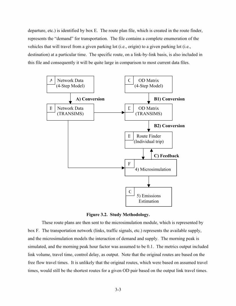
3-3

departure, etc.) is identified by box E. The route plan file, which is created in the route finder,

represents the “demand” for transportation. The file contains a complete enumeration of the

vehicles that will travel from a given parking lot (i.e., origin) to a given parking lot (i.e.,

destination) at a particular time. The specific route, on a link-by-link basis, is also included in

this file and consequently it will be quite large in comparison to most current data files.

Figure 3.2. Study Methodology.

These route plans are then sent to the microsimulation module, which is represented by

box F. The transportation network (links, traffic signals, etc.) represents the available supply,

and the microsimulation models the interaction of demand and supply. The morning peak is

simulated, and the morning peak hour factor was assumed to be 0.1. The metrics output included

link volume, travel time, control delay, as output. Note that the original routes are based on the

free flow travel times. It is unlikely that the original routes, which were based on assumed travel

times, would still be the shortest routes for a given OD pair based on the output link travel times.

A) Conversion B1) Conversion

B2) Conversion

C) Feedback

Network Data (4-Step Model)

A

Network Data (TRANSIMS)

B

OD Matrix (4-Step Model)

C

OD Matrix (TRANSIMS)

D

Route Finder (Individual trip)

E

4) 4) Microsimulation F

5) Emissions Estimation

G

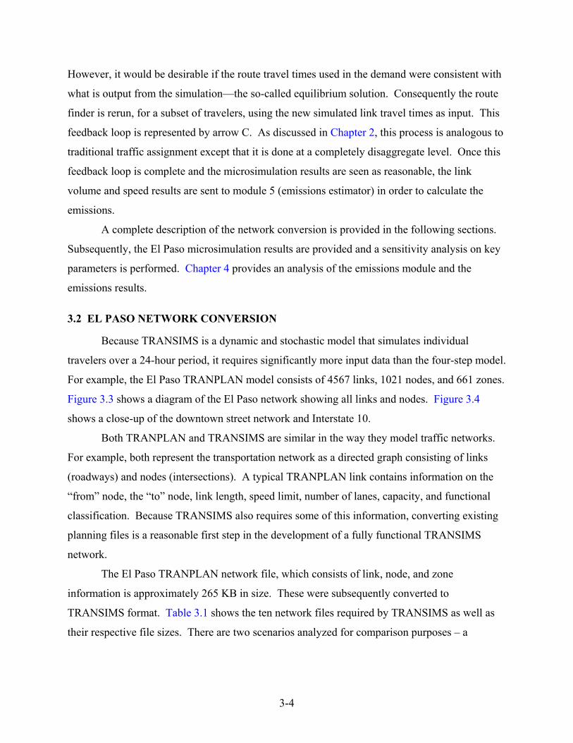
3-4

However, it would be desirable if the route travel times used in the demand were consistent with

what is output from the simulation—the so-called equilibrium solution. Consequently the route

finder is rerun, for a subset of travelers, using the new simulated link travel times as input. This

feedback loop is represented by arrow C. As discussed in Chapter 2, this process is analogous to

traditional traffic assignment except that it is done at a completely disaggregate level. Once this

feedback loop is complete and the microsimulation results are seen as reasonable, the link

volume and speed results are sent to module 5 (emissions estimator) in order to calculate the

emissions.

A complete description of the network conversion is provided in the following sections.

Subsequently, the El Paso microsimulation results are provided and a sensitivity analysis on key

parameters is performed. Chapter 4 provides an analysis of the emissions module and the

emissions results.

3.2 EL PASO NETWORK CONVERSION

Because TRANSIMS is a dynamic and stochastic model that simulates individual

travelers over a 24-hour period, it requires significantly more input data than the four-step model.

For example, the El Paso TRANPLAN model consists of 4567 links, 1021 nodes, and 661 zones.

Figure 3.3 shows a diagram of the El Paso network showing all links and nodes. Figure 3.4

shows a close-up of the downtown street network and Interstate 10.

Both TRANPLAN and TRANSIMS are similar in the way they model traffic networks.

For example, both represent the transportation network as a directed graph consisting of links

(roadways) and nodes (intersections). A typical TRANPLAN link contains information on the

“from” node, the “to” node, link length, speed limit, number of lanes, capacity, and functional

classification. Because TRANSIMS also requires some of this information, converting existing

planning files is a reasonable first step in the development of a fully functional TRANSIMS

network.

The El Paso TRANPLAN network file, which consists of link, node, and zone

information is approximately 265 KB in size. These were subsequently converted to

TRANSIMS format. Table 3.1 shows the ten network files required by TRANSIMS as well as

their respective file sizes. There are two scenarios analyzed for comparison purposes – a

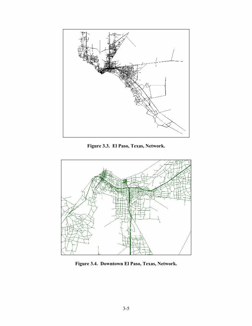
3-5

Figure 3.3. El Paso, Texas, Network.

Figure 3.4. Downtown El Paso, Texas, Network.

3-6

network with no pocket lanes and a network with pocket lanes. The network details will be

described in greater detail in later sections of this report. The size of each file is also shown, and

it can be seen that considerably more data storage is required for TRANSIMS than TRANPLAN.

This reflects the greater informational requirement for TRANSIMS as well as the fact that the

information is typically stored at the individual element level rather than aggregated. For

example, the individual links comprising the route every traveler will take as they journey from

their origin link to their destination link is stored. In contrast, TRANPLAN only stores the

aggregate OD demand, and the routes are calculated endogenously as part of the traffic

assignment step. Each file type, along with the underlying conversion process, will be discussed

in detail in the following sections.

Table 3.1. Required El Paso TRANSIMS Files.

TRANSIMS Files

No Pocket Lane

Scenario (KB)

Pocket Lane Scenario

(KB)

Node (ELPASO_NODE.tbl) 106 106

Link (ELPASO_LINK.tbl) 1488 1488

Pocket Lane (ELPASO_POCKET.tbl) 0.1 160

Lane Connectivity (ELPASO_CONNECTIVITY.tbl) 623 740

Parking Lot (ELPASO_PARKING.tbl) 133 133

Unsignalized Control (ELPASO_UNSIGNALIZED.tbl) 8 8

Signalized Control (ELPASO_SIGNALIZED.tbl) 48 48

Signal Timing (ELPASO_TIMING.tbl) 0.4 0.4

Phasing (ELPASO_PHASING.tbl) 465 465

Study Area (ELPASO_STUDYAREA.tbl) 79 79

TOTAL 2950.5 3227.4

3.2.1 Node and Link Information Conversion

Table 3.2 shows the attributes of the TRANSIMS node file. It can be seen that there are

three attributes: Node ID, X-Coordinate, and Y-Coordinate and these are directly analogous to

the TRANPLAN attributes. Because there was a direct relationship the conversion was

relatively straightforward.

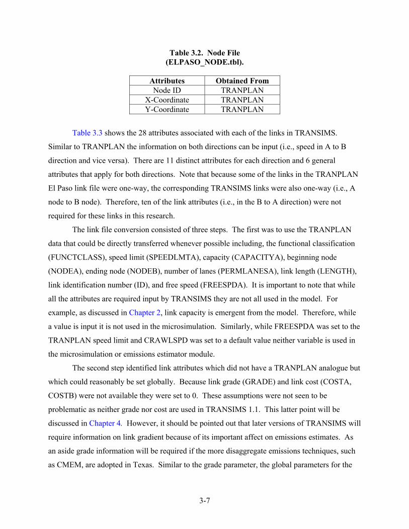
3-7

Table 3.2. Node File (ELPASO_NODE.tbl).

Attributes Obtained From Node ID TRANPLAN

X-Coordinate TRANPLAN Y-Coordinate TRANPLAN

Table 3.3 shows the 28 attributes associated with each of the links in TRANSIMS.

Similar to TRANPLAN the information on both directions can be input (i.e., speed in A to B

direction and vice versa). There are 11 distinct attributes for each direction and 6 general

attributes that apply for both directions. Note that because some of the links in the TRANPLAN

El Paso link file were one-way, the corresponding TRANSIMS links were also one-way (i.e., A

node to B node). Therefore, ten of the link attributes (i.e., in the B to A direction) were not

required for these links in this research.

The link file conversion consisted of three steps. The first was to use the TRANPLAN

data that could be directly transferred whenever possible including, the functional classification

(FUNCTCLASS), speed limit (SPEEDLMTA), capacity (CAPACITYA), beginning node

(NODEA), ending node (NODEB), number of lanes (PERMLANESA), link length (LENGTH),

link identification number (ID), and free speed (FREESPDA). It is important to note that while

all the attributes are required input by TRANSIMS they are not all used in the model. For

example, as discussed in Chapter 2, link capacity is emergent from the model. Therefore, while

a value is input it is not used in the microsimulation. Similarly, while FREESPDA was set to the

TRANPLAN speed limit and CRAWLSPD was set to a default value neither variable is used in

the microsimulation or emissions estimator module.

The second step identified link attributes which did not have a TRANPLAN analogue but

which could reasonably be set globally. Because link grade (GRADE) and link cost (COSTA,

COSTB) were not available they were set to 0. These assumptions were not seen to be

problematic as neither grade nor cost are used in TRANSIMS 1.1. This latter point will be

discussed in Chapter 4. However, it should be pointed out that later versions of TRANSIMS will

require information on link gradient because of its important affect on emissions estimates. As

an aside grade information will be required if the more disaggregate emissions techniques, such

as CMEM, are adopted in Texas. Similar to the grade parameter, the global parameters for the

3-8

presence of a two-way left-turn lane (TWOWAYTURN) and color (COLOR) were assumed both

to be zero. Note that it would be relatively easy to code the color by functional classification.

As well, the two-way left-turn lane is not available in this version of TRANSIMS.

Table 3.3. Link File (ELPASO_LINK.tbl).

Attributes Directional

Attribute Obtained from:

NODEA TRANPLAN NODEB TRANPLAN PERMLANESA TRANPLAN THRUA Conversion3 LEFTPCKTSA Conversion3 RGHTPCKTSA Conversion3 SPEEDLMTA TRANPLAN FREESPDA TRANPLAN CRAWLSPDA 8.94 mi/h 1 SETBACKA Conversion3 CAPACITYA TRANPLAN2 COSTA 01 PERMLANESB TRANPLAN THRUB Conversion3 LEFTPCKTSB Conversion3 RGHTPCKTSB Conversion3 SPEEDLMTB TRANPLAN FREESPDB TRANPLAN CRAWLSPDB 8.94 mi/h 1 SETBACKB Conversion3 CAPACITYB TRANPLAN2 COSTB 01 ID No TRANPLAN LENGTH No TRANPLAN FUNCTCLASS No TRANPLAN GRADE No 01 COLOR No 01 TWOWAYTURN No 01

1 Global assumption for all links. 2 Taken from TRANPLAN file but not used in TRANSIMS. 3 Converted from TRANPLAN file. Actual value depends on link

attributes.

3-9

The third step was the most complicated because it involved estimating link attributes

that did not exist in the TRANPLAN files and could not reasonably be set globally. One of the

most critical is the presence of pocket lanes. Figure 3.5 shows a schematic diagram of pocket

lanes. The lanes can be placed at either end of a link in both directions. Pocket lanes may be

considered turning bays on arterial type streets and merge/diverge lanes on freeways.

Figure 3.5. Schematic Diagram of a Pocket Lane.

Because there were not enough resources to empirically enumerate the turning bays (and

their attributes) these attributes were estimated. Basically any links downstream of an on-ramp

had a pocket lane added at its upstream end to model the merging of traffic. Similarly any links

upstream of an on-ramp had a pocket lane added to the downstream end to model the diverging

maneuver. On the street network all links that had a functional classification of arterial roadway

had left and right pocket lanes added to their downstream ends to model left-turning behavior.

The estimation of the pocket lane is problematic as it could add capacity to the system that might

not actually exist.

The link file does not contain the necessary detail to fully describe the pocket lanes, and

therefore a pocket lane file, shown in Table 3.4, is required. The information that was input was

consistent with the conversion methodology discussed previously. The LINK and NODE

attribute information are consistent with the link file. A unique identifier (ID) was added for

Pocket Lane Pocket Lane

Pocket Lane Pocket Lane

Pocket Lane Length ~ f (roadway type, link length)

3-10

each pocket lane. The length of the pocket lane (LENGTH) was estimated as the lesser of one

half the link length or 200 m (i.e., six-vehicle length). The offset is in reference to the

downstream node, and for turn lanes this was set to zero. The style refers to the type of pocket

lane used, and this is a function of whether the link is on the street or highway network.

In TRANSIMS the link and lane choices drivers face as they come to the end of a lane

need to be explicitly enumerated. This is done through the lane connectivity table that

enumerates which lanes on the downstream links a driver on a given lane can use. The driver is

prohibited from using any lane/link combination not contained in this table.

Table 3.4. Pocket Lane File (ELPASO_POCKET.tbl).

Attribute Obtained from: OFFSET Function of merge/diverge lane2 LENGTH Function of link length2 LINK TRANPLAN3 ID Unique identifier2 LANE Function of link type1 NODE TRANPLAN3 STYLE Function of link type1

1 Default values used in conversion process. 2 Assigned in conversion process. 3 Consistent with link file.

Figure 3.6 shows a hypothetical example of lane connectivity. Consider a vehicle

traveling down link A. If the vehicle is in lane A1 it would only be allowed to continue on to

link C using only lane C1. In contrast, if the vehicle were traveling in lane A2 it could continue

on to link C (lane C2) or link D (lane D1). If the vehicle entered the pocket lane (lane PA1) it

could turn left onto link B using lane B1.

Needless to say it is critically important for the lane connectivity to be correct. The route

selection algorithm uses the lane connectivity file to identify the link/lane combinations that a

particular vehicle will use to get from its origin to its destination. Obviously, poor or inaccurate

connections, such as allowing a left turn movement from lane A2 to lane B1, could potentially

lead to spurious results. In addition, if difficult or impossible maneuvers are added it will lead to

errors in the microsimulation. For example, if a driver wished to turn onto lane B1 of link B but

3-11

could not get over in time to enter the pocket lane, the microsimulator would simply remove the

vehicle from the simulation (LANL, 2000).

The calculation of the lane connectivity for the El Paso network was a two-step process.

The first step was to identify the potential downstream links and the type of movement (i.e., left

turn, through movement, right turn) required to enter them. Identifying the number of

downstream links was relatively straightforward in that it was a simple enumeration of the links

which have a given link’s end node as their beginning node. However, identifying the type of

turn was a bit more challenging. In this situation an algorithm was written that identified the

vectors for the upstream and downstream links. The angle between the vectors was calculated,

and the turn type was calculated based on this angle. Figure 3.7 shows a conceptualization of

this process. For a given upstream link, if the relative angle was less than 120 degrees it was a

right turn, if it was greater than 240 degrees it was a left turn, and anything else was a through

movement.

3-12

Figure 3.6. Lane Connectivity Example.

PA1

A1

A2

B1

C1

C2

D1Link A

Link D

Link C

Link B

3-13

Figure 3.7. Turning Movement Example.

The second step was to identify the lane connectivity between the links. Similar to the

pocket lane analysis it was impractical to collect empirical data for the entire El Paso network.

Instead an algorithm was developed to automatically connect the lanes based on the number of

lanes on the upstream link, the number of downstream links, the number of lanes in each

downstream link, the presence and type of pocket lanes, and the type of turning movements

identified in the first step. In general through lanes were connected, left lanes (or left pocket

lanes) were connected to the leftmost lane of the downstream link for left turns, and right lanes

(or right pocket lanes) were connected to the rightmost lane of the downstream link for right

turns.

Table 3.5 shows the lane connectivity file format. Basically there is a line for each lane

of each link, and it shows the link and the lane with which it is connected. Needless to say

identifying the link connectivity empirically would be problematic as the requirements are very

Through Movement

Right Turn

Left Turn

Upstream Link

3-14

data intensive. It is unlikely any traffic department, let alone a metropolitan planning

organization, would have this data available. In order for TRANSIMS to be applied at a

practical level a comprehensive database would have to be developed, perhaps as part of a larger

geographic information system (GIS), or the conversion process would have to be automated as

was done in this research.

Table 3.5. Lane Connectivity File (ELPASO_CONNECTIVITY.tbl).

Attribute Obtained From NODE TRANPLAN2 INLINK TRANPLAN2 INLANE Lane number2 OUTLINK TRANPLAN2 OUTLANE Lane identifier1

1 Assigned in conversion process. 2 Consistent with TRANSIMS node and/or

link file.

3.2.2 Traffic Signal Control

In addition to identifying the lane connectivity, the type of signal control at the end of

each link needs to be identified. In the case of signalized intersections the attributes of the signal

timing plan need to be described in detail. Similar to the link connectivity problem there were

not enough resources to collect empirical information on the traffic signal control at every

intersection. Consequently this process was automated as well.

The first step was to identify the type of intersection at the end of each link. For

freeways this is relatively straightforward as they are modeled as a series of connected, uni-

directional links. Consequently, there are no signal controls at the end of these links. For the

arterial roadway network the process was more complicated. First, researchers identified the

presence of an intersection based on the presence of conflicting links and their angle to each

other. Depending on the functional classification of the intersecting roads the type of

intersection was identified. For example, if a collector road intersected with an arterial road then

it was assumed that the collector was stop controlled. In contrast, the intersection of an arterial

roadway and an arterial roadway was assumed to be controlled by a traffic signal.

3-15

Table 3.6 shows the input of the unsignalized intersection attribute file. For each node in

the network the type of control (stop, yield, uncontrolled) for each inbound link is defined.

Table 3.7 shows the attributes required for the intersections that are signalized. This file

indicates which node is signalized, the type of signalization, which plan it is running, the time

the plan starts, and the offset. These latter two are set to zero in this research indicating that

there is no coordination across traffic signals. It was assumed that all traffic signals operated on

fixed time because the peak hour was being modeled.

Table 3.6. Unsignalized Intersection File

(ELPASO_UNSIGNALIZED.tbl).

Attribute Obtained from: NODE INLINK SIGN

TRANPLAN2 TRANPLAN2 Function of Link Class1

1 Assigned in conversion process. 2 Consistent with node and/or link file.

Table 3.7. Signalized Intersection File (ELPASO_SIGNALIZED.tbl).

Attribute

Obtained from:

NODE TRANPLAN3 TYPE T1 PLAN 1,2, or 32 Function of link types OFFSET 01 START TIME 0:001

1 Default values used in conversion process. 2 Assigned in conversion process. 3 Consistent with node file.

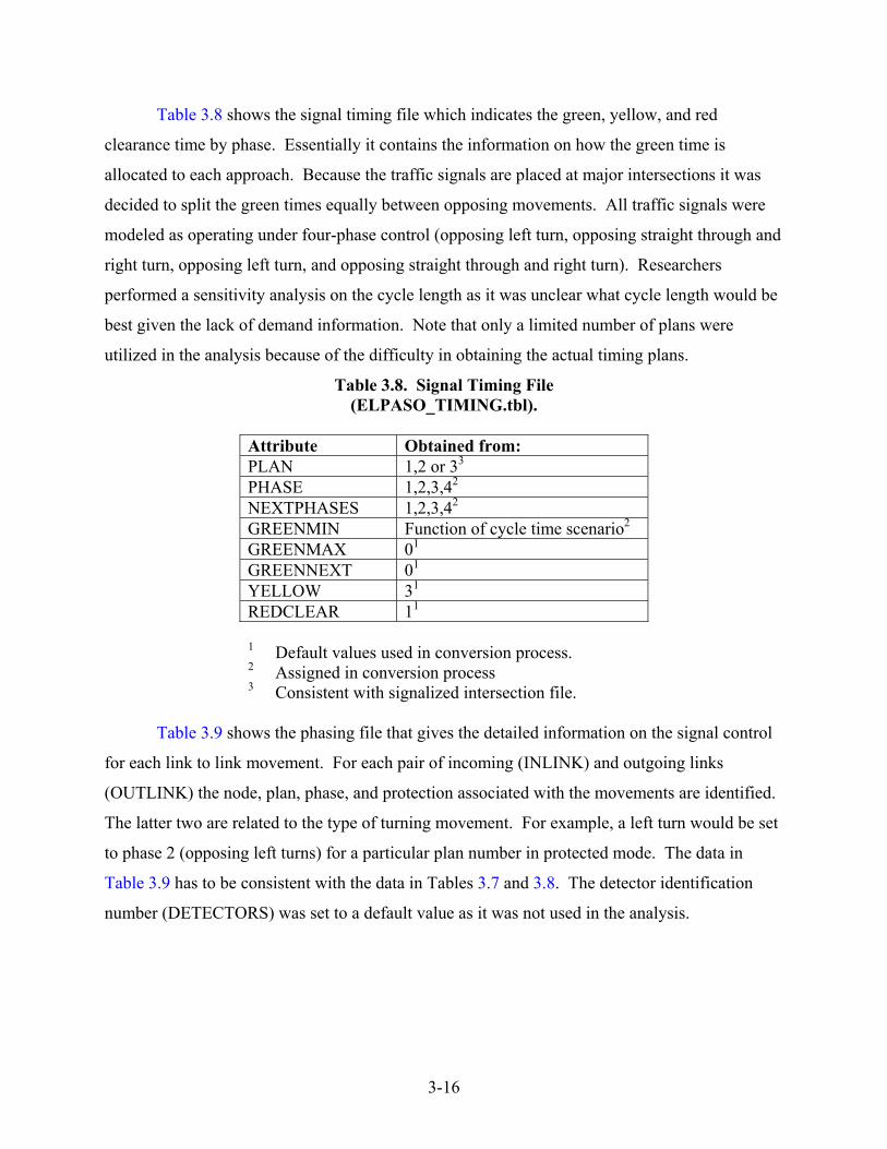
3-16

Table 3.8 shows the signal timing file which indicates the green, yellow, and red

clearance time by phase. Essentially it contains the information on how the green time is

allocated to each approach. Because the traffic signals are placed at major intersections it was

decided to split the green times equally between opposing movements. All traffic signals were

modeled as operating under four-phase control (opposing left turn, opposing straight through and

right turn, opposing left turn, and opposing straight through and right turn). Researchers

performed a sensitivity analysis on the cycle length as it was unclear what cycle length would be

best given the lack of demand information. Note that only a limited number of plans were

utilized in the analysis because of the difficulty in obtaining the actual timing plans.

Table 3.8. Signal Timing File (ELPASO_TIMING.tbl).

Attribute Obtained from: PLAN 1,2 or 33 PHASE 1,2,3,42 NEXTPHASES 1,2,3,42 GREENMIN Function of cycle time scenario2 GREENMAX 01 GREENNEXT 01 YELLOW 31 REDCLEAR 11

1 Default values used in conversion process. 2 Assigned in conversion process 3 Consistent with signalized intersection file.

Table 3.9 shows the phasing file that gives the detailed information on the signal control

for each link to link movement. For each pair of incoming (INLINK) and outgoing links

(OUTLINK) the node, plan, phase, and protection associated with the movements are identified.

The latter two are related to the type of turning movement. For example, a left turn would be set

to phase 2 (opposing left turns) for a particular plan number in protected mode. The data in

Table 3.9 has to be consistent with the data in Tables 3.7 and 3.8. The detector identification

number (DETECTORS) was set to a default value as it was not used in the analysis.

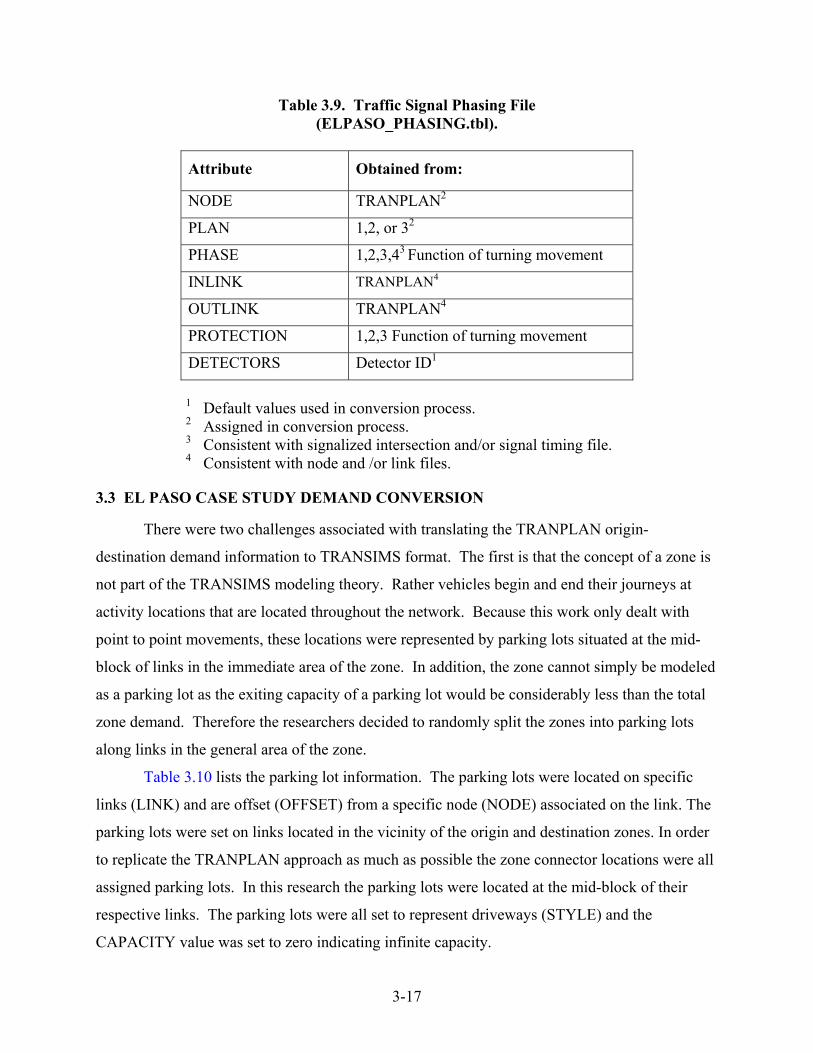
3-17

Table 3.9. Traffic Signal Phasing File (ELPASO_PHASING.tbl).

Attribute Obtained from:

NODE TRANPLAN2

PLAN 1,2, or 32

PHASE 1,2,3,43 Function of turning movement

INLINK TRANPLAN4

OUTLINK TRANPLAN4

PROTECTION 1,2,3 Function of turning movement

DETECTORS Detector ID1

1 Default values used in conversion process. 2 Assigned in conversion process. 3 Consistent with signalized intersection and/or signal timing file. 4 Consistent with node and /or link files.

3.3 EL PASO CASE STUDY DEMAND CONVERSION

There were two challenges associated with translating the TRANPLAN origin-

destination demand information to TRANSIMS format. The first is that the concept of a zone is

not part of the TRANSIMS modeling theory. Rather vehicles begin and end their journeys at

activity locations that are located throughout the network. Because this work only dealt with

point to point movements, these locations were represented by parking lots situated at the mid-

block of links in the immediate area of the zone. In addition, the zone cannot simply be modeled

as a parking lot as the exiting capacity of a parking lot would be considerably less than the total

zone demand. Therefore the researchers decided to randomly split the zones into parking lots

along links in the general area of the zone.

Table 3.10 lists the parking lot information. The parking lots were located on specific

links (LINK) and are offset (OFFSET) from a specific node (NODE) associated on the link. The

parking lots were set on links located in the vicinity of the origin and destination zones. In order

to replicate the TRANPLAN approach as much as possible the zone connector locations were all

assigned parking lots. In this research the parking lots were located at the mid-block of their

respective links. The parking lots were all set to represent driveways (STYLE) and the

CAPACITY value was set to zero indicating infinite capacity.

3-18

Table 3.10. Parking File (ElPASO_PARKING.tbl).

Attribute Obtained from: GENERIC T1

OFFSET TRANPLAN (Mid-link) 1

CAPACITY 01

LINK TRANPLAN (Link ID) 3

ID TRANPLAN3

NODE TRANPLAN3

STYLE DRVWY1 (driveway)

ZONE Zone ID4

1 Default values used in conversion process 2 Consistent with node and link files. 3 Consistent with TRANPLAN zone information.

Table 3.11. Study Area File (ELPASO_STUDYAREA.tbl).

Attribute Obtained from:

ID Link ID2

BUFFER 0,11

1 Default values used in conversion process. 2 Consistent with node and link files.

Once the parking lots associated with each zone were identified a representative fraction

of the demand was assigned to travel between these parking lots. If aggregated the total parking

lot to parking lot demand would equal the zone to zone demand. The individual vehicle

movements were translated from the aggregated parking lot to parking lot demand randomly and

dispersed throughout the simulation period. For example, if the demand from parking lot A to

3-19

parking lot B was 10 vehicles then 10 individual vehicles would be generated with departure

times spaced randomly throughout the hour based on a Poisson distribution with a mean time of

six minutes.

The second challenge was to create the individual plans or routes that these vehicles

would follow. This required the demand information (as described by the point to point

movement of all the individual vehicles as well as the supply information (link connectivity and

link attributes). A shortest-path algorithm was used to calculate the route on a link (and lane) by

link (and lane) basis. By the time the OD information was disaggregated to individual vehicles

and a separate path identified for each vehicle, the original TRANPLAN OD file increased from

500 KB to 50 MB.

3.4 EL PASO MICROSIMULATION RESULTS

The 1997 El Paso network consists of 4567 links and is 1539.2 km in length. There are

13 link types in the network, and the functional classification is shown in Table 3.12. Figure 3.8

shows the number of links by functional classification while Figure 3.9 shows the network km by

functional classification. The principal roadways modeled are freeways (including ramps and

frontage roads), arterial roadways, and collectors which account for approximately 16, 40, and 7

percent of the network, respectively. The local roads are modeled by the zone connectors which

account for approximately 36 percent of the network.

Once the network and demand files were created TRANSIMS was run using the

methodology shown previously in Figure 3.2. Specifically the input was fed into the

microsimulation module (box F) and the output was obtained. While the demand was assumed

to be constant the drivers were modeled as having the capability of changing their routes (box E).

In order to avoid oscillations because of every traveler changing their routes in response to

updated travel times, it was decided to only allow a fraction of the vehicles to reroute at any one

iteration. Note that the TRANSIMS route planner module was not available in version 1.1 so the

plans were created using a simple routing program. The process was iterated until the aggregate

results were stabilized and at each iteration 10 percent of the drivers were given new routes. The

decision to only consider aggregate values, such as total system travel time, was adopted because

the concept of user equilibrium does not exist in dynamic and stochastic networks of the type

modeled by TRANSIMS. Therefore, it was decided to use a stability metric to judge how well a

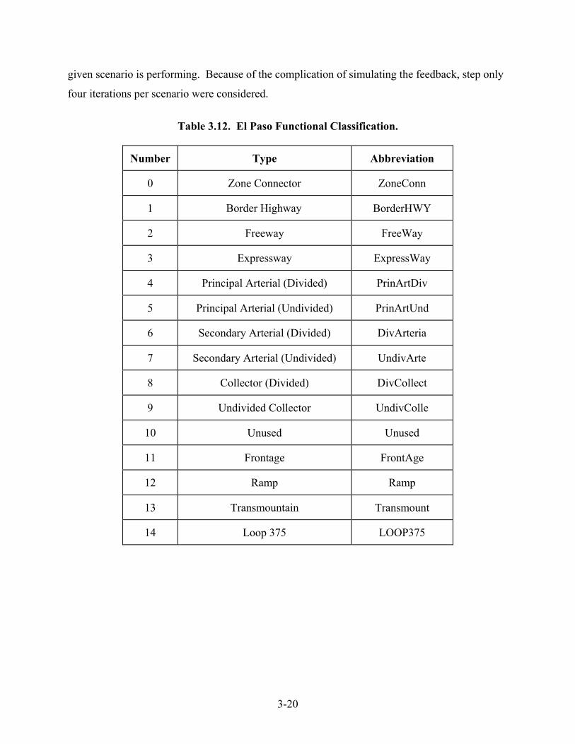
3-20

given scenario is performing. Because of the complication of simulating the feedback, step only

four iterations per scenario were considered.

Table 3.12. El Paso Functional Classification.

Number Type Abbreviation

0 Zone Connector ZoneConn

1 Border Highway BorderHWY

2 Freeway FreeWay

3 Expressway ExpressWay

4 Principal Arterial (Divided) PrinArtDiv

5 Principal Arterial (Undivided) PrinArtUnd

6 Secondary Arterial (Divided) DivArteria

7 Secondary Arterial (Undivided) UndivArte

8 Collector (Divided) DivCollect

9 Undivided Collector UndivColle

10 Unused Unused

11 Frontage FrontAge

12 Ramp Ramp

13 Transmountain Transmount

14 Loop 375 LOOP375

3-21

0

200

400

600

800

1000

1200

1400

1600

1800

ZoneC

onn

BorderH

WY

FreeW

ay

Expres

sWay

PrinArtD

iv

PrinArtU

nd

DivArte

ria

UndivA

rte

DivColl

ect

UndivC

olle

FrontAge

Ramp

Transm

ount

LOOP37

5

Functional Classification

Num

ber o

f Lin

ks

Figure 3.8. El Paso Functional Classification Histogram.

0

100

200

300

400

500

600

700

800

900

1000

ZoneC

onn

BorderH

WY

FreeW

ay

Expres

sWay

PrinArtD

iv

PrinArtU

nd

DivArte

ria

UndivA

rte

DivColl

ect

UndivC

olle

FrontA

geRam

p

Transm

ount

LOOP37

5

Functional Classification

Kilo

met

ers

Figure 3.9. El Paso Network Length by Functional Classification.

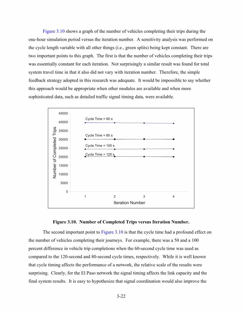
3-22

Figure 3.10 shows a graph of the number of vehicles completing their trips during the

one-hour simulation period versus the iteration number. A sensitivity analysis was performed on

the cycle length variable with all other things (i.e., green splits) being kept constant. There are

two important points to this graph. The first is that the number of vehicles completing their trips

was essentially constant for each iteration. Not surprisingly a similar result was found for total

system travel time in that it also did not vary with iteration number. Therefore, the simple

feedback strategy adopted in this research was adequate. It would be impossible to say whether

this approach would be appropriate when other modules are available and when more

sophisticated data, such as detailed traffic signal timing data, were available.

Figure 3.10. Number of Completed Trips versus Iteration Number.

The second important point to Figure 3.10 is that the cycle time had a profound effect on

the number of vehicles completing their journeys. For example, there was a 50 and a 100

percent difference in vehicle trip completions when the 60-second cycle time was used as

compared to the 120-second and 80-second cycle times, respectively. While it is well known

that cycle timing affects the performance of a network, the relative scale of the results were

surprising. Clearly, for the El Paso network the signal timing affects the link capacity and the

final system results. It is easy to hypothesize that signal coordination would also improve the

0

5000

10000

15000

20000

25000

30000

35000

40000

45000

1 2 3 4

Iteration Number

Num

bero

fCom

plet

edTr

ips

Cycle Time = 60 s

Cycle Time = 80 s

Cycle Time = 100 s

Cycle Time = 120 s

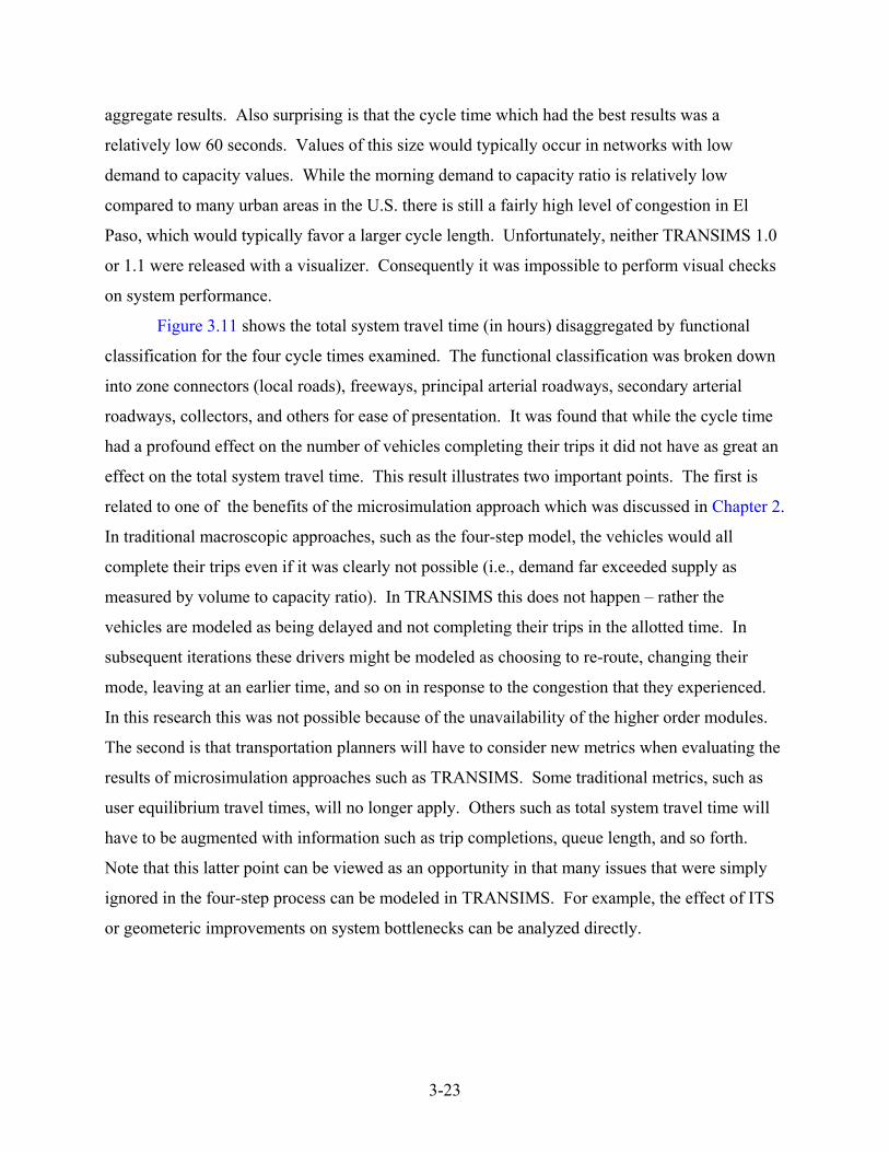
3-23

aggregate results. Also surprising is that the cycle time which had the best results was a

relatively low 60 seconds. Values of this size would typically occur in networks with low

demand to capacity values. While the morning demand to capacity ratio is relatively low

compared to many urban areas in the U.S. there is still a fairly high level of congestion in El

Paso, which would typically favor a larger cycle length. Unfortunately, neither TRANSIMS 1.0

or 1.1 were released with a visualizer. Consequently it was impossible to perform visual checks

on system performance.

Figure 3.11 shows the total system travel time (in hours) disaggregated by functional

classification for the four cycle times examined. The functional classification was broken down

into zone connectors (local roads), freeways, principal arterial roadways, secondary arterial

roadways, collectors, and others for ease of presentation. It was found that while the cycle time

had a profound effect on the number of vehicles completing their trips it did not have as great an

effect on the total system travel time. This result illustrates two important points. The first is

related to one of the benefits of the microsimulation approach which was discussed in Chapter 2.

In traditional macroscopic approaches, such as the four-step model, the vehicles would all

complete their trips even if it was clearly not possible (i.e., demand far exceeded supply as

measured by volume to capacity ratio). In TRANSIMS this does not happen – rather the

vehicles are modeled as being delayed and not completing their trips in the allotted time. In

subsequent iterations these drivers might be modeled as choosing to re-route, changing their

mode, leaving at an earlier time, and so on in response to the congestion that they experienced.

In this research this was not possible because of the unavailability of the higher order modules.

The second is that transportation planners will have to consider new metrics when evaluating the

results of microsimulation approaches such as TRANSIMS. Some traditional metrics, such as

user equilibrium travel times, will no longer apply. Others such as total system travel time will

have to be augmented with information such as trip completions, queue length, and so forth.

Note that this latter point can be viewed as an opportunity in that many issues that were simply

ignored in the four-step process can be modeled in TRANSIMS. For example, the effect of ITS

or geometeric improvements on system bottlenecks can be analyzed directly.

3-24

0

1000

2000

3000

4000

5000

6000

7000

8000

9000

ZoneConnectors

Freeways PrincipalArterials

SecondaryArterials

Collector Others

Functional Classification

Tota

l Tra

vel T

ime

(hou

rs) 60

80100120

Cycle Time

Figure 3.11. Total Travel Time by Functional Classification

The bulk of the total travel time is experienced on the local streets (i.e., zone connectors)

which is not surprising given that 1) these roadways account for 36 percent of the network size,

and 2) that all trips either begin or end at a parking lot located on these facilities. Note that

principal arterial roadways have the greatest contribution to the total system travel time with both

freeways and secondary arterial roadways experiencing approximately the same amount of travel

time. These findings reflect the larger scope of the arterial roadways in the El Paso network and

the better performance of the freeway system in that it is less congested in relation to the street

system. It is hypothesized that the relatively high values of congestion on the street network is

the result of poor signal location and/or timing rather than something explicitly related to the El

Paso network. More accurate data or better estimation techniques could reduce the estimated

travel time on these facilities. This result again indicates the importance of proper data before

the results from these detailed microsimulation systems can be used with confidence.

3-25

3.5 LESSONS LEARNED

There are a number of lessons identified in this chapter and these are summarized below:

1. TRANSIMS requires substantially more and different input data than the four-step process. The amount of data required for TRANSIMS is considerably more than for TRANPLAN. While TRANPLAN keeps all network information on a single file, TRANSIMS employs 12 files for this purpose. In the case of the El Paso network the original TRANPLAN file was approximately 400 KB in size while the converted files – without the addition of the local roads – was on the order of 3,340 KB in size.

2. Estimation techniques will need to be developed for some of the input data not currently collected. Because TRANSIMS models transportation supply in much more detail, more information is required, and this information is often not readily available. For example, unlike TRANPLAN, both pocket lane (i.e., turning bays) locations and pocket lane length are required by TRANSIMS. In addition, the allowable movements from each lane on a given link to all the downstream lanes that it connects to needs to be defined explicitly in lane connectivity tables. For the El Paso case study heuristic algorithms were used to populate the pocket lane and lane connectivity data fields.

Perhaps more problematic is that traffic signal information (i.e., location and timing plans) is required in TRANSIMS but is not available in TRANPLAN data sets. If this information is available at all, it is often stored by different agencies and/or departments. Needless to say it will not be a small task to collect this information for the base year model and to predict this information for future year scenarios.

There are two potential solutions to the above problems. The first solution would be to develop a comprehensive database, perhaps in the form of a geographic information system. Detailed geometric and traffic control information could be stored in a centralized way for use by traffic engineers, design professionals, and transportation planners. The second solution would be to use standard signal optimization programs, such as TRANSYT 7-F and PASSER III, to estimate the signal timing plans and offsets. However, these programs require approach volumes. Consequently, if these signal optimization programs were employed then a feedback loop would be required to ensure that the assumed approach volumes were consistent with the modeled approach volumes. To the author’s knowledge this type of feedback has never been studied, and the viability of such an approach is unclear.

3. TRANSIMS will require more sophisticated error checking than the four-step

model. TRANSIMS calculates the travel demand internally, and therefore OD tables from existing files will not need to be converted. However, existing OD files are useful for comparing the supply relationships of the models by assuming constant travel “demand” as was done in the Dallas, Texas, case study. Because each traveler’s route is defined explicitly, the routing files are very large. Another problem with the conversion is that error-checking requirements are increased considerably. In TRANSIMS release 1.1, which was used in the research described in this report, there is literally no

3-26

error-checking capability and the problems in converting network files are myriad. Because the final release will have error-checking capability, techniques for addressing this issue were not discussed in detail.

4. Future year forecasts will have to be more sophisticated than presently used.

TRANSIMS was designed to model individual households, which means that the traditional concept of zones does not apply to TRANSIMS. In effect, each household is modeled as a separate entity, and therefore zones and zone collector information can be eliminated. However, transportation modelers will need to obtain detailed network information on the local streets for future years. Needless to say, how best to estimate this type of future data is an open and important research topic.

5. TRANSIMS can be implemented in an incremental manner in Texas. There are two

basic approaches for implementing TRANSIMS. The first is to use the full version where all five modules are employed. This would entail a significant amount of preparation and the implementation effort would be substantial. The second is to utilize the superior supply modeling, and in particular the traffic microsimulation and emissions estimation modules, together with demand represented by OD matrices obtained from a traditional four-step model. This was the approach adopted in this research. It was shown that it was possible to develop the more complex network files and demand files from existing data files. It should be noted that it was difficult to definitively examine the quality of the TRANSIMS results because 1) the traffic signal locations were based on an algorithmic process, 2) the traffic signal timings were not coordinated, 3) the lane connectivity and pocket lane information were developed through the use of an algorithmic process, and 4) the graphical user interface is not included in version 1.1 and consequently a visual check of the network and assignment could not be done. The results showed that TRANSIMS was sensitive to different signal timing characteristics and geometric conditions. The potential benefit is a more realistic representation of traffic conditions than would be obtainable from traditional macroscopic link speed-volume relationships that are currently used. For example, changes in traffic operations (i.e., ITS), geometric characteristics (additional lanes on ramps), and/or physical capacity (i.e., new roadways) could be modeled in a consistent and realistic manner – something that is not possible using the four-step model.

4-1

CHAPTER 4–EMISSIONS ESTIMATION

The emissions estimator module is used to estimate fuel consumption and pollutant

emissions, hydrocarbon (HC), carbon monoxide (CO), and nitrogen oxides (NOx), associated

with a particular traffic microsimulation run. The methodology is disaggregate in nature

although the input is aggregated over space (i.e., 30 m sections of roadway) and time (i.e., one

hour).

This chapter will focus on the theory behind the emissions estimator module. The

procedure will be illustrated using the microsimulation results described in Chapter 3. The first

section of the chapter describes the TRANSIMS emissions estimation procedure. The next

section examines the emissions methodology of the MOBILE suite of models which is the

current state of the practice for estimating emissions in Texas. A comparison between the two

approaches is provided. Lastly, the results from the El Paso test case are provided and discussed.

4.1 TRANSIMS EMISSIONS ESTIMATOR MODULE

There are many factors which affect emissions rates including vehicle type, engine status,

vehicle speed, vehicle acceleration, and vehicle power demand (Barth et al., 1997). For example,

when a vehicle experiences a very hard acceleration the engine enters an enrichment phase in

which it releases more than a normal amount of pollutants. Greater than normal emissions can

also be experienced when a vehicle travels uphill on a steep grade even if it simply maintains its

speed. The CMEM model can estimate emissions for individual vehicles provided detailed

information on acceleration, speed, power, and so on are available (Barth et al., 1997). Because

of its ability to model all components of the driving cycle it was used as the basis of the

TRANSIMS methodology. While the TRANSIMS low fidelity microsimulation may accurately

represent aggregate traffic dynamics it clearly does not estimate the detailed information required

by CMEM as was demonstrated in Chapter 2. Consequently, the developers of TRANSIMS

decided to augment the aggregate output from the microsimulation with empirical information on

power demands experienced under typical traffic conditions. This approach was shown in

Figure 2.1 where the emissions estimator is shown as a separate module and is run after the

microsimulation stage is complete. Figure 4.1 shows the light-duty vehicle (LDV) estimation

module and it can be seen that there are three inputs to the emissions module: 1) fleet

composition, 2) fleet status, and 3) fleet dynamics.

4-2

Figure 4.1. Light-Duty Vehicle Emissions Estimation Methodology

4.1.1 Fleet Composition

The fleet composition, as shown by box 1 in Figure 4.1, typically would be developed

within the population synthesizer module. That is, the attributes of the synthetic individuals and

households also would include the type and characteristics of their vehicle(s). These attributes

would be derived from vehicle registration data, inspection and maintenance testing, or data

developed for input to the MOBILE5a emissions model. In the full version of TRANSIMS there

are 28 vehicle categories. As shown in Table 4.1 these categories are based on vehicle

classification, emissions control technology, type of fuel system, emissions standard level, power

Microsimulation Results 1) Fleet Composition Synthetic Vehicle Population

2) Fleet Status • 3 levels of soak

time • 8 levels of

“start/stop” cycles

3) Fleet Dynamics • 30 m segments • 1 hour duration • Six speed bins • (0,1,2,3,4,5 cells/s or 0,

16.8, 33.6, 50.3, 67.1, 83.9 mph)

4) LDV Aggregate Dynamic Submodule

• 30 m segments • 1 hour duration • 20 speed bins (4 mph

increments) • 34 power ratios

5) LDV Tailpipe Emissions • Fuel consumption • HC, CO, NOx

4-3

to weight ratio and emitter level (Barth et al., 1997). Because the population synthesizer was not

used in this research all emissions estimates are based on the default vehicle types which are

representative of the fleet in southern California. Because the vehicle fleet in TRANSIMS 1.1,

which was used in this research, is composed entirely of light-duty vehicles, this chapter

primarily will focus on the emissions estimation for this type of vehicle.

4.1.2 Fleet Status

The second input, fleet status, is a measure of when and where the vehicles on a given

link have been operating. This is shown as box 2 in Figure 4.1, and the information is obtained

from the microsimulation results. The vehicles are classified in two ways. The first

categorization is by soak time, which is the amount of time between the current start of operation

and the last trip. In the full version of TRANSIMS there are three soak times’ categories: 20

minutes, one hour, and five hours. For each soak time group the vehicles are further divided by

the integrated product of speed and acceleration since their engine was started for the current

trip. The integrated product of speed and acceleration are analogous to start/stop cycles as will

be discussed later. There are eight categories where the first group represents vehicles with cold

engines (i.e., highest polluting), and the eighth group represents vehicles with optimally warm

engine temperatures (i.e., lowest polluting). In summary, the fleet status is a three by eight table

containing the proportion of simulated vehicles in each of the 24 categories that operate on a

given link for each hour of simulation time.

Table 4.1. Vehicle Categories.

No. Category/Type 1 Normal emitting, no catalyst car 2 High emitting, no catalyst car 3 Normal emitting, 2-way catalyst car 4 High emitting, 2-way catalyst car 5 Normal emitting, 3-way catalyst, carbureted car 6 High emitting, 3-way catalyst, carbureted car 7 Normal emitting, 3-way catalyst with fuel injection, >50K miles, low power/weight car 8 Normal emitting, 3-way catalyst with fuel injection, >50K miles, high power/weight car 9 Normal emitting, 3-way catalyst with fuel injection, <50K miles, low power/weight car 10 Normal emitting, 3-way catalyst with fuel injection, <50K miles, high power/weight car 11 High emitting, 3-way catalyst with fuel injection car 12 Normal emitting, Tier 1, >50K miles, low power/weight car 13 Normal emitting, Tier 1, >50K miles, high power/weight car

4-4

No. Category/Type 14 Normal emitting, Tier 1, <50K miles, low power/weight car 15 Normal emitting, Tier 1, <50K miles, high power/weight car 16 High emitting, Tier 1 car 17 Normal emitting, Pre-1979 (<=8500 gross vehicle weight) truck 18 High emitting, Pre-1979 (<=8500 gross vehicle weight) truck 19 Normal emitting, 1979-1983 (<=8500 gross vehicle weight) truck 20 High emitting, 1979-1983 (<=8500 gross vehicle weight) truck 21 Normal emitting, 1984-1987 (<=8500 gross vehicle weight) truck 22 High emitting, 1984-1987 (<=8500 gross vehicle weight) truck 23 Normal emitting, 1988-1993 (<=3750 loaded vehicle weight) truck 24 Normal emitting, 1988-1993 (>3750 loaded vehicle weight) truck 25 High emitting, 1988-1993 truck 26 Normal emitting, Tier 1, LDT2/3 (3751-5750 loaded vehicle weight or Alt. loaded

vehicle weight) truck 27 Normal emitting, Tier 1, LDT4 (6001-8500 gross vehicle weight, > 5750 Alt. loaded

vehicle weight) truck 28 High emitting Tier 1 truck

The objective of grouping the vehicles in this manner is to identify the fraction of

vehicles on each link still suffering from the effects of cold engine starts or which are operating

below the optimal catalyst temperature. In general, the colder the engine the higher the

emissions and fuel consumption. In addition, the longer the soak time the longer it takes for the

engine and catalyst to reach the optimal temperature. The LDVs (i.e., gasoline-fueled passenger

cars) tailpipe emissions estimator, which is indicated by box 5 in Figure 4.1, calculates the

emissions for traffic on the network assuming that all vehicles are at the optimal engine

temperature. The base emissions estimates subsequently are adjusted to reflect the status of the

vehicles on the link.

There is a separate multiplier for each parameter (i.e., HC, CO, NOx, and fuel

consumption) for each of the 24 groups. The multiplier represents the percent increase (or

decrease) in pollutants coming from vehicles in that stage of engine warm-up relative to an

optimally warm engine. These multipliers are based on empirical measurements of vehicles in

the southern California area. These vehicles followed a specific trajectory, which involved

starting from a near stop, accelerating to a typical arterial roadway speed, and then decelerating

to a near stop (U.S. Environmental Protection Agency, 1993). The same trajectory was repeated

over 10 cycles. The Comprehensive Modal Emissions Model (Barth et al., 1997) was used to

estimate the emissions associated with the empirical driving trajectories. The LANL researchers

4-5

calculated these emissions assuming four different soak times: 0 minutes, 20 minutes, 1 hour,

and 5 hours. The emissions for the non-zero soak times were compared to the emissions for the

zero soak time, and the pollutant multipliers were calculated for each of the eight start/stop

cycles and three soak time combinations. Specific details of the procedure for calculating these

multipliers may be found elsewhere (Williams et al., 1999).

The only multipliers released in TRANSIMS version 1.1 were for the one-hour soak time

and these are shown in Figure 4.2. It can be seen that for HC and CO as the number of start/stop

cycles increases (i.e., the engines became warmer) the multiplier for pollutants generally

decreases. For example, the HC multiplier for the first start/stop group is 2.7 and decreases to 1

for the eighth start/stop cycle. Note that the multiplier for the eighth start/stop cycle for all

parameters is 1 indicating that the engine is at the optimally warm temperature. In general, the

CO emissions multiplier follows a similar pattern to HC although the multipliers are smaller.

Interestingly, the CO multiplier for the fifth and sixth start/stop cycle is less than 1 indicating the

cooler engine in this range produces less CO emissions than the fully warmed engine, all else

being equal. In contrast, the NOx multiplier decreases until the fourth start/stop cycle after

which it increases up to the seventh start/stop cycle. The fuel consumption multiplier ranges

from 1.07 to 1.1 indicating that the fuel consumption for a non-optimally warm engine ranges

from 7 to 10 percent higher than that of an optimally warm engine. However, fuel consumption

is least affected by start/stop cycle as evidenced by the relatively small multiplier values and the

fact that there is no discernible relationship between the multiplier and the start/stop cycle.

0

0.5

1

1.5

2

2.5

3

1 2 3 4 5 6 7 8Start/Stop Cycle

Emis

sion

Mul

tiplie

r

HCCONOxFuel Consumption

Figure 4.2. Emissions Multiplier for One Hour Soak Time by Start/Stop Cycle.

4-6

4.1.3 Fleet Dynamics

The third input, fleet dynamics, refers to the microsimulation output and is shown by

box 3 in Figure 4.1. The individual vehicle data from the microsimulation is aggregated both

spatially (e.g., into 30 m segments along each link) and temporally (e.g., sixty-minute time

intervals).

For each 30 m block the number of vehicles that experience a given speed (over one

second) are counted and output. There are six speed bins as shown in Table 4.2 and range from

0 to 5 cells/s (0-83.9 mph) in increments of 1 cell/s (16.8 mph). Note that the count is not simply

the volume crossing the block. Rather it represents the number of vehicles in a given 30 m block

experiencing a given speed over a one-second period. For example, if a vehicle traveled across a

given 30 m (4 cell) block at a speed of 1 cell/s then four observations would be added to the

1 cell/s speed bin counter. Conversely, if the vehicle traveled at a speed of 4 cells/s then one

observation would be added to the 4 cells/s speed bin counter.

Table 4.2. Link to Velocity Summary File (emissions.vel file).

Name Definition LINK Link ID being reported. NODE Node ID from which the vehicles were traveling away. DISTANCE Ending distance of the box (in meters) from the setback of the node from

which the vehicles were traveling away. TIME Current time (seconds from midnight). COUNT0 Number of vehicles with velocities in the range (0, 7.5). COUNT1 Number of vehicles with velocities in the range (7.5, 15). COUNT2 Number of vehicles with velocities in the range (15, 22.5). COUNT3 Number of vehicles with velocities in the range (22.5, 30). COUNT4 Number of vehicles with velocities in the range (30, 37.5). COUNT5 Number of vehicles with velocities in the range (37.5, infinity).

Vehicle speeds are given in steps per second. Conversion rates to mi/h are given in Table 2.1.

As mentioned earlier the relationships between emissions, speed, and power are highly

non-linear. In addition, the TRANSIMS microsimulation output is not detailed enough to model

acceleration and power at an individual vehicle level. Because the microsimulation module only

provides average conditions over an hour period at fixed points in space the LDV Aggregate

Dynamic Submodule (box 4 in Figure 4.1) was developed to translate this information into

detailed power estimates that could be used to model emissions. Basically the distribution of

4-7

hard accelerations (where the engine enters enrichment) and the distribution of hard

decelerations for vehicles on all types of roadways including freeways, arterials, collector, and so

forth are estimated from the microsimulation output. From this the power requirements are

derived as measured by the product of speed and acceleration. A separate methodology was

developed for estimating the power requirements for vehicles accelerating after stopping at a

traffic signal and for vehicles which accelerate as they proceed down an on-ramp.

The translation process consists of two parts. One translation consists of approximating a

continuous speed distribution from the discrete speed input data shown in Table 4.2. A series of

line segments is used to approximate the desired distribution. The end result is that the vehicles

in the six speed bins (0,1…5 cells/s) are translated into 20 speed bins which have ranges of

4 mph (0-4, 4-8, 8-12). In addition, the proportion of vehicles in each speed bin that are

experiencing a specific power demand, as measured by the velocity-acceleration product, is

required. Empirical test vehicle data from the EPA were used to develop the relationship

between the aggregate data and the required power estimates (U.S. EPA, 1993). It is important

to note that it is the tails of the power (i.e., acceleration and speed product) distribution that are

the focus of the estimation procedure because of the relatively high emissions rates associated

with vehicles operating under these conditions.

Most of the vehicles are assumed to have an insignificant power requirement as measured

by the velocity acceleration product. In essence, they are assumed to have the same pollutant

emissions rate as vehicles that are traveling at a constant velocity. Of course, the emissions vary

according to the value of the constant velocity.

A proportion of the vehicles are modeled as having higher (lower) emissions because

they are experiencing higher (lower) power demands. For example, high power demands for

vehicles experiencing a positive acceleration are “defined by velocity-acceleration greater than

50 mph squared per second which corresponds with the 10 percent point on the cumulative

distribution” (LANL, 2000). These 10 percent of the vehicles are further subdivided into 15

equal high power categories. The vehicles in the 15 high power categories are modeled

separately, even though their proportion of the total number of vehicles is quite low, because

1) the power rates within the 15 have considerable variation in emissions rates, and 2) all 15

categories have considerably higher emissions rates than vehicles that are not experiencing

“significant” changes in speed. The LANL researchers conducted a similar analysis to model

4-8

vehicles experiencing a hard deceleration. A velocity acceleration product higher than 50 mph

squared per second is considered the threshold for high power and a product of –50 is the

threshold for low power. Note that the methodology explicitly accounts for congestion. For

example, a greater portion of vehicles will be modeled as experiencing hard accelerations and

decelerations on a congested network than on an uncongested network. Empirical data on

individual LDV trajectories on different types of roadways were used to develop the appropriate

equations (Effa and Larson, 1993). In addition, the methodology also accounts for grade effects.

Because TRANSIMS 1.1 did not have this capability it is not described in this report, and this is

why the default value of the grades were set to zero. A detailed description of the methodology

for translating the aggregate microsimulation speed output into detailed

speed/acceleration/power output may be found elsewhere (Williams et al., 1999).

Figure 4.1 shows that the output of the LDV Aggregate Dynamic Submodule is an array

which contains a count of the vehicles in each 30 m segment over a one-hour period which are

categorized as belonging to one of 20 four-mph speed bins and one of 34 different power levels

based on their acceleration speed product (i.e., power). Of these 34 different power levels, 18

are high power levels, 15 are low power levels, and one is an insignificant power level. Note

that, in general, the majority of vehicles will belong to this last category. This 20 by 34 array is

calculated for each 30 m segment of roadway and is input to the LDV emissions estimator.

For every power level there is a corresponding emissions rate for each pollutant. The

CMEM model was used to develop the emissions rates for each cell of the corresponding speed –

power levels (Barth et al., 1997). That is, there is a separate emissions rate for each of the 20

speed bins and each of the 34 power levels. The emissions rates were based on factors including

proportions of vehicles with higher mileage, catalyst type, model year, power-to-weight ratio,

and so forth. The synthetic vehicle population, box 1 in Figure 4.1, is used to obtain this

information and, as discussed previously, the default parameters were used. In addition, the

difference in emissions between vehicles with constant power trajectories and those with the

same speed and power, but with a step change in power over the previous second, is calculated.

Researchers used this information to address history effects. A detailed description of the

emissions estimation methodology may be found elsewhere (LANL, 2001).

The concepts discussed above are best represented graphically. Figure 4.3 shows the

relationship between acceleration and speed for six representative power levels. Each function

4-9

represents a constant power level where power is defined as the product of acceleration and

speed and the units are in mph2/s. For example, point A on the topmost function represents an

acceleration of 50 mph/s and a speed of 6 mph (i.e., the midpoint of the 4-8 mph speed bin)

which corresponds to a power of 300 mph2/s. Every point on this topmost function has the same

power value of 300 mph2/s. The -300, -180, and -60 mph2/s power levels correspond to the 15th,

9th, and 3rd low power levels, respectively. These functions all represent vehicles undergoing a

deceleration. The 60, 180, and 300 mph2/s power levels correspond to the 3rd, 9th, and 15th power

-150

-100

-50

0

50

100

150

2 6 10 14 18 22 26 30 34 38 42 46 50 54 58 62 66 70 74 78

Speed (mph)

Acc

eler

atio

n (m

ph/s

)

-300 -180-6060180300

Power (mph2/s)

A

Figure 4.3. Power versus Speed Bin.

levels, respectively and represent vehicles undergoing an acceleration. The -300, -180 and -60

mph2/s power levels are mirror images of the 300, 180, and 60 mph2/s power levels, respectively.

As would be expected, as the speed increases the absolute value of the acceleration decreases and

tends to level off at the higher speeds. Therefore, vehicles that are allocated to the higher speed

bins will have a correspondingly lower absolute value of acceleration. Note that the

acceleration-speed function for the insignificant power level (i.e., the ones most vehicles will be

allocated to) is equal to zero indicating that the vehicles in this group do not have power

demands that would adversely affect the emissions rates.

The fuel consumption rate versus speed bin is shown in Figure 4.4. It can be seen that for

the vehicles experiencing decelerations the fuel consumption is constant up to the 60-64 mph

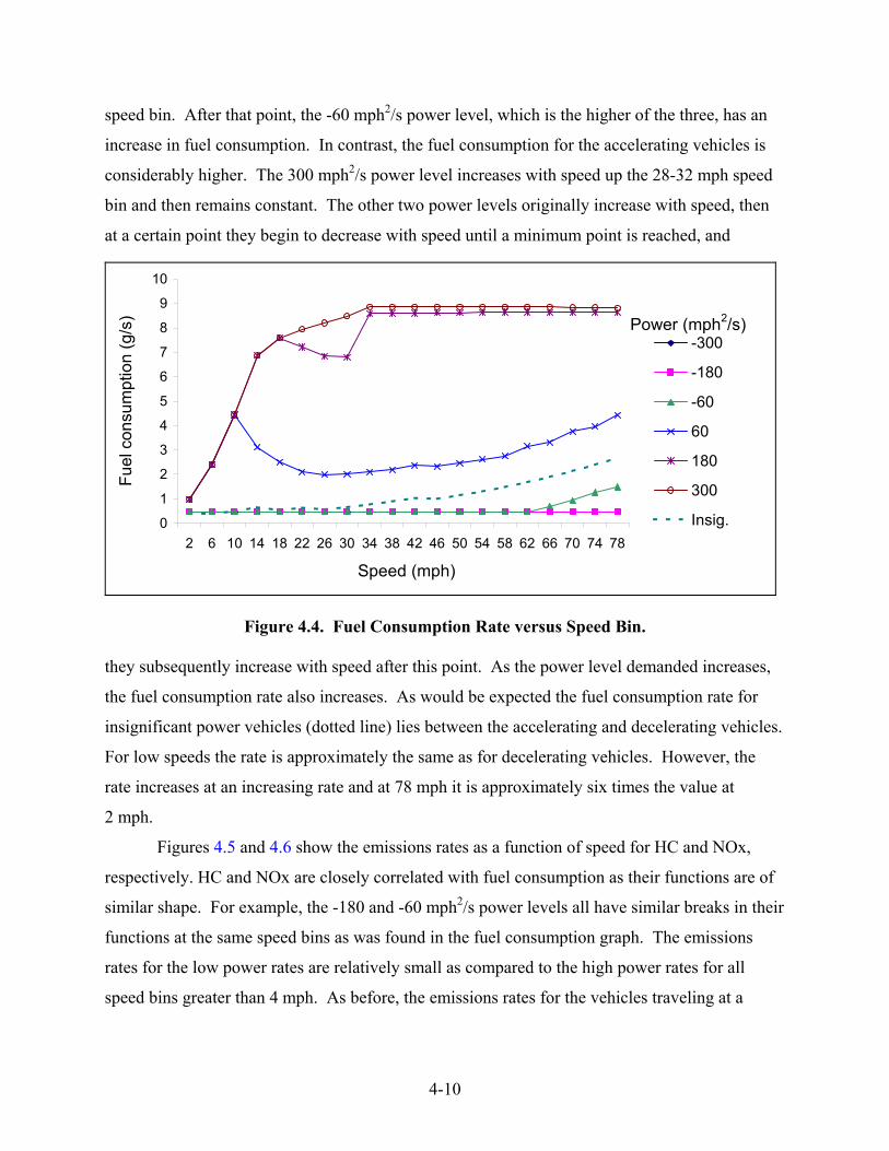
4-10

speed bin. After that point, the -60 mph2/s power level, which is the higher of the three, has an

increase in fuel consumption. In contrast, the fuel consumption for the accelerating vehicles is

considerably higher. The 300 mph2/s power level increases with speed up the 28-32 mph speed

bin and then remains constant. The other two power levels originally increase with speed, then

at a certain point they begin to decrease with speed until a minimum point is reached, and

0

1

2

3

4

5

6

7

8

9

10

2 6 10 14 18 22 26 30 34 38 42 46 50 54 58 62 66 70 74 78

Speed (mph)

Fuel

con

sum

ptio

n (g

/s)

-300

-180

-60

60

180

300

Insig.

Power (mph2/s)

Figure 4.4. Fuel Consumption Rate versus Speed Bin. they subsequently increase with speed after this point. As the power level demanded increases,

the fuel consumption rate also increases. As would be expected the fuel consumption rate for

insignificant power vehicles (dotted line) lies between the accelerating and decelerating vehicles.

For low speeds the rate is approximately the same as for decelerating vehicles. However, the

rate increases at an increasing rate and at 78 mph it is approximately six times the value at

2 mph.

Figures 4.5 and 4.6 show the emissions rates as a function of speed for HC and NOx,

respectively. HC and NOx are closely correlated with fuel consumption as their functions are of

similar shape. For example, the -180 and -60 mph2/s power levels all have similar breaks in their

functions at the same speed bins as was found in the fuel consumption graph. The emissions

rates for the low power rates are relatively small as compared to the high power rates for all

speed bins greater than 4 mph. As before, the emissions rates for the vehicles traveling at a

4-11

constant speed (insignificant power requirement) lie between the rates for the accelerating and

decelerating vehicles.

Figure 4.5. NOx Emissions Rate versus Speed Bin.

Figure 4.6. CO Emissions Rate versus Speed Bin.

0

0.02

0.04

0.06

0.08

0.1

0.12

0.14

0.16

2 6 10 14 18 22 26 30 34 38 42 46 50 54 58 62 66 70 74 78

Speed (mph)

NO

x E

mis

sion

Rat

e (g

/s)

-300 -180-6060180300Insig.

Power (mph2/s)

0

1

2

3

4

5

6

7

8

2 6 10 14 18 22 26 30 34 38 42 46 50 54 58 62 66 70 74 78

Speed (mph)

CO

Em

issi

on R

ate

(g/s

)

-300 -180-6060180300Insig.

Power (mph2/s)

4-12

The HC emissions rate as a function of speed for the six representative power levels is

shown in Figure 4.7. The deceleration relationships start off relatively high as compared to the

acceleration scenarios and decrease with speed bin. In contrast, the accelerating vehicles

increase with speed bin, achieve a maximum value, and then decrease. Note that the highest

power relationship has two peaks: one at the 16-20 mph speed bin and the other at the 32-36 mph

speed bin. The highest rates of emissions for the highest power levels, 180 mph2/s and

300 mph2/s, occur between 10 and 38 mi/h. The HC emissions rates for the vehicles

experiencing constant speed (or insignificant power requirements) are relatively constant and

approximately equal to the rates for the vehicles with low deceleration values.

0

0.2

0.4

0.6

0.8

1

1.2

1.4

1.6

2 6 10 14 18 22 26 30 34 38 42 46 50 54 58 62 66 70 74 78Speed (mph)

HC

Em

issi

on R

ate

(g/s

)

-300 -180-6060180300Insig.

Power (mph2/s)

Figure 4.7. HC Emissions Rate versus Speed Bin.

Figures 4.5 through 4.7 illustrate the highly non-linear relationship between emissions

rate, power (i.e., acceleration-speed product), and speed. Simply using the aggregate speed value

for a given section of roadway over a specific period of time would not be appropriate. In

general, the emissions estimate would be underestimated considerably. This is an illustration of

the mathematical concept that “the function of the average is not equal to the average of the

function.” The important point is that if the TRANSIMS developers had simply used an average

acceleration/power for all vehicles on the link, together with the CMEM emissions model, they

would have seriously underestimated emissions. Consequently, they developed a methodology

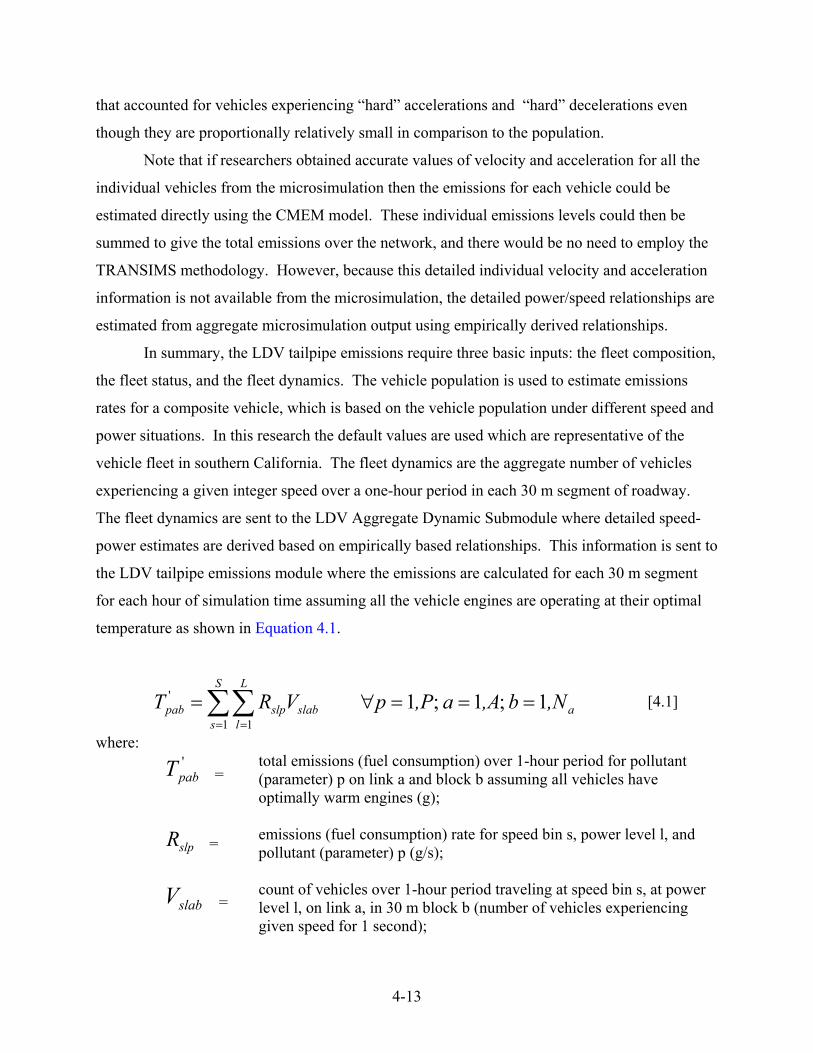
4-13

that accounted for vehicles experiencing “hard” accelerations and “hard” decelerations even

though they are proportionally relatively small in comparison to the population.

Note that if researchers obtained accurate values of velocity and acceleration for all the

individual vehicles from the microsimulation then the emissions for each vehicle could be

estimated directly using the CMEM model. These individual emissions levels could then be

summed to give the total emissions over the network, and there would be no need to employ the

TRANSIMS methodology. However, because this detailed individual velocity and acceleration

information is not available from the microsimulation, the detailed power/speed relationships are

estimated from aggregate microsimulation output using empirically derived relationships.

In summary, the LDV tailpipe emissions require three basic inputs: the fleet composition,

the fleet status, and the fleet dynamics. The vehicle population is used to estimate emissions

rates for a composite vehicle, which is based on the vehicle population under different speed and

power situations. In this research the default values are used which are representative of the

vehicle fleet in southern California. The fleet dynamics are the aggregate number of vehicles

experiencing a given integer speed over a one-hour period in each 30 m segment of roadway.

The fleet dynamics are sent to the LDV Aggregate Dynamic Submodule where detailed speed-

power estimates are derived based on empirically based relationships. This information is sent to

the LDV tailpipe emissions module where the emissions are calculated for each 30 m segment

for each hour of simulation time assuming all the vehicle engines are operating at their optimal

temperature as shown in Equation 4.1.

a

S

s

L

lslabslppab ,Nb,Aa,PpVRT 1 ;1 ;1

1 1

' ===∀= ∑∑= =

[4.1]

where: '

pabT = total emissions (fuel consumption) over 1-hour period for pollutant (parameter) p on link a and block b assuming all vehicles have optimally warm engines (g);

slpR = emissions (fuel consumption) rate for speed bin s, power level l, and

pollutant (parameter) p (g/s);

slabV =

count of vehicles over 1-hour period traveling at speed bin s, at power level l, on link a, in 30 m block b (number of vehicles experiencing given speed for 1 second);

4-14

Na = number of 30 m blocks on link a;

S = number of speed bins (i.e., 20);

L = number of power levels (i.e., 34);

A = number of links in network; and

P = number of parameters (i.e., 4 – HC, NOx, CO, and fuel consumption).

These emissions are subsequently adjusted using multipliers which account for the fact

that different parts of the fleet will have engine temperatures that are non-optimal as shown in

Equation 4.2.

a

C

i

C

jpabijpabpab ,Nb,Aa,PpMTT

s T

1 ;1 ;1 1 1

' ===∀= ∑∑= =

[4.2]

where:

pabijM = multiplier rate for pollutant (parameter p), link a, block b, start/stop cycle category i, and soak time j;

Cs = number of start/stop cycle categories (8); and

CT = number of soak time categories (3 – 1 in TRANSIMS 1.1).

The data can subsequently be aggregated over the entire network as shown in Equation 4.3.

,PpTTA

a

N

bpabp

a

1 1 1

' =∀= ∑∑= =

[4.3]

where:

pT = total emissions (fuel consumption) over 1-hour period over entire network for parameter p.

Note that the analyst can aggregate the data in any number of ways such as link type,

time of day, and so forth as will be demonstrated later in this chapter.

4.2 THE MOBILE5A EMISSIONS MODEL

The MOBILE5a vehicular emissions model, developed by the Environmental Protection

Agency was used for comparison purposes. The researchers used MOBILE5a in this study

4-15

because it has been widely adopted across North America. MOBILE6, which has recently been

released can be considered an improvement on MOBILE5a because its emissions rates are

developed for a number of different roadway types and for different levels of congestion.

Additionally, MOBILE6 makes it possible to model on-cycle and off-cycle emissions. The basic

logic and building blocks of the two models are the same, however, so it is hypothesized that the

general research results will also be applicable for MOBILE6.

The basic emissions rates for MOBILE5a were determined through actual vehicle tests on

a dynamometer. The rollers of the dynamometer apply forces to the drive wheels of the vehicle

to simulate the loading experienced in actual driving conditions. Vehicles are “driven” through

the standard federal testing procedure (FTP) drive cycle, which is designed to be indicative of

driving patterns in urban areas. Emissions for various vehicle classes, model years, and operating

conditions are recorded with special measuring equipment. Basic emissions rate equations are

then developed for each pollutant, vehicle type and model year (U.S. Environmental Protection

Agency, 2002).

MOBILE5a uses a variety of factors related to the specified conditions to convert the

basic emissions rates into final emissions rates. Note that these functions are not widely

published and most were identified directly from the MOBILE5a source code (Jordan, 1996;

Cottrell, 1992). The pollutants examined in this research are hydrocarbons, carbon monoxide,

and nitrogen oxides. The composite emissions rate for a given pollutant type, vehicle class,

model year and speed is derived as the product of the basic emissions rate and a number of

correction factors that are related to the model years and operating characteristics of the vehicles.

The general relationship for computing the MOBILE5a emissions rate is shown in Equation 4.4.

,J,P; j,Y; p,N; yiDHSRFCBC iyiyiyiyiyiypjiypiypj 1111 1 ====∀+++++= where: iypjC1 = composite emissions rate for vehicle class i, model year y, pollutant

p, and speed index j (g/km);

iypB = base emissions rate for vehicle class i, model year y, and pollutant p (g/km);

iypjC = composite correction factor for vehicle class i, model year y, pollutant p, and speed index j ;

iyF = refueling factor for vehicle class i and model year y ( p = HC);

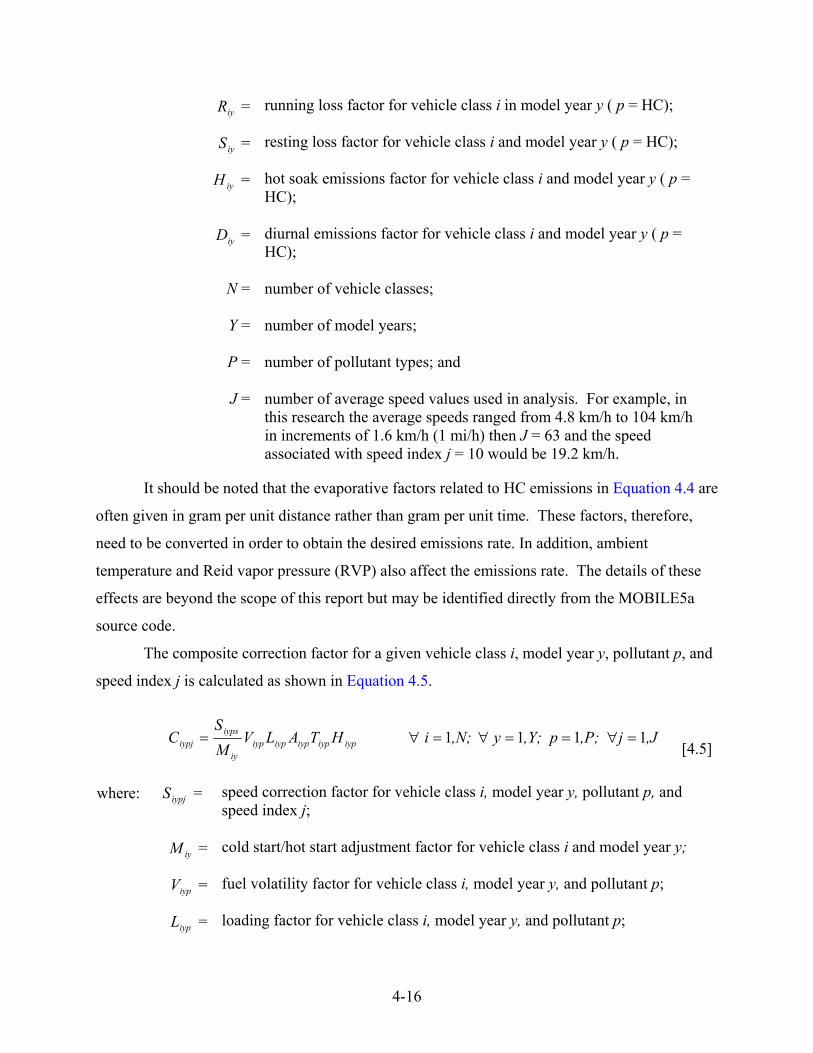
4-16

iyR = running loss factor for vehicle class i in model year y ( p = HC);

iyS = resting loss factor for vehicle class i and model year y ( p = HC);

iyH = hot soak emissions factor for vehicle class i and model year y ( p = HC);

iyD = diurnal emissions factor for vehicle class i and model year y ( p = HC);

N = number of vehicle classes;

Y = number of model years;

P = number of pollutant types; and

J = number of average speed values used in analysis. For example, in this research the average speeds ranged from 4.8 km/h to 104 km/h in increments of 1.6 km/h (1 mi/h) then J = 63 and the speed associated with speed index j = 10 would be 19.2 km/h.

It should be noted that the evaporative factors related to HC emissions in Equation 4.4 are

often given in gram per unit distance rather than gram per unit time. These factors, therefore,

need to be converted in order to obtain the desired emissions rate. In addition, ambient

temperature and Reid vapor pressure (RVP) also affect the emissions rate. The details of these

effects are beyond the scope of this report but may be identified directly from the MOBILE5a

source code.

The composite correction factor for a given vehicle class i, model year y, pollutant p, and

speed index j is calculated as shown in Equation 4.5.

,Jj,P; ,Y; p y ,N; iHTALVMS

C iypiypiypiypiypiy

iypsiypj 111 1 =∀==∀=∀=

[4.5]

where: iypjS = speed correction factor for vehicle class i, model year y, pollutant p, and speed index j;

iyM = cold start/hot start adjustment factor for vehicle class i and model year y;

iypV = fuel volatility factor for vehicle class i, model year y, and pollutant p;

iypL = loading factor for vehicle class i, model year y, and pollutant p;

4-17

iypA = air conditioning factor for vehicle class i, model year y, and pollutant p;

iypT = trailer towing factor for vehicle class i, model year y, and pollutant p; and

iypH = humidity factor for vehicle class i, model year y, and pollutant p (p= NOX).

The speed correction factor is shown in Equation 4.6. Note that these equations apply

only to post-1976 model years and other functions are used for earlier model years.

( )x

2

x

NO ;1

11 543exp

)NO1 ;1

11 21

==∀

=∀=∀++=

≠=∀=∀

=∀=∀+=

p,Jj

,Y; y,N; iskskkS

,P (p p ,Jj

,Y; y,N; iks

kS

jiypjjiypjiypjiypj

iypjj

iypjiypj

[4.6]

where: js = speed associated with speed index j (km/h).

The cold start/hot start adjustment factor for a given vehicle class i and model year y is

calculated using Equation 4.7.

YyNixwxw

M iyiyiyiyiy ,1 ;,1

161

26

1

==∀

−−+

+=

−

[4.7]

where: iyw = fraction of vehicle class i and model year y in hot start mode, and

iyx = fraction of vehicle class i and model year y in cold start mode. Once the composite emissions rate, iypjC1 , is identified an aggregate emissions rate by

pollutant and vehicle class is calculated as shown in Equation 4.8.

JjPpNizCCY

yiyjiypjipj ,1 ;,1 ;,1 12

1===∀= ∑

=

[4.8]

where: ipjC2 = composite emissions rate for vehicle class i, pollutant p, and speed index j (g/km); and

iyjz = fraction of total vehicle kilometers of travel VKT for vehicle class i contributed by model year y for speed index j.

4-18

It is important to note that emissions on a gram-per-second basis are not calculated in the

MOBILE5a model. The emissions rates are developed in terms of grams of pollutant per

distance traveled, because vehicle kilometers of travel and average speed per link can be

obtained from the output of transportation planning models. The total amount of pollutant p

emitted in a given traffic network can, therefore, readily be calculated by summing the product

of the emissions rate and the vehicle kilometers of travel for each vehicle class (categorized by

average speed) as shown in Equation 4.9.

∑∑= =

=∀=N

i

J

jijipjp PpvCT

1 1,1 2

[4.9]

where: ijv = vehicle kilometers of travel for vehicle class i traveling at the speed associated with speed index j. Note that the VKT implicitly assumes a time unit (i.e., per month, per year); and

pT = total amount of pollutant p produced (g). Note that this is expressed in the same units (i.e., per month, per year) as ijv .

Given the eight vehicle classifications, three pollutants, 50 model years, and the large

number of causal variables, the task of writing out all of the equations in the MOBILE5a model

would be quite burdensome. Consequently a computer program has been written to perform the

calculations for the analyst.

While the emissions rates used in Equation 4.9 are calculated for an individual test

vehicle traveling at an average speed, there is no standard protocol for identifying the VKT for

each vehicle class i and speed j ( ijv ). Typically, a macroscopic four-step transportation model is

used to identify ijv , and there are two important points related to this fact. The first is that for a

given link the recorded VKT by vehicle class is based on an average speed for all vehicle classes

because only one speed value per link is output. That is, unlike TRANSIMS, MOBILE5a only

considers average speed conditions. Secondly, there are no specifications on the appropriate link

length or time interval for analyses purposes. This potentially could be problematic because the

average speed used in Equation 4.5 will be a function of the temporal and spatial aggregation

length used to calculate the average speed.

4-19

Because the goal is to compare the two models the TRANSIMS output will be used as

input to the MOBILE5a model. Specifically, the traffic data will be aggregated by link over a

one-hour period. The average speed and the volume of vehicles on each link will be output.

Similar to the TRANSIMS study only LDVs will be considered. It should be noted that for the

El Paso network LDVs make up 93, 99, and 91 percent of the vehicle mix on the collectors,

arterial roadways, and freeways, respectively as shown in Figure 4.8. The component emissions

rates, as defined in Equation 4.4, will be used for the analysis. These rates were obtained from

MOBILE5a and do reflect El Paso specific factors including vehicle type, proportion of vehicles

in cold start, and so on. Subsequently, Equation 4.10 will be used to calculate the total emissions

by pollutant for each link using the link volume and average speed output from the TRANSIMS

microsimulation module.

,A,P; apLCV

Ta

paapa 11 ==∀=

[4.10]

where: paC = MOBILE5a LDV composite emissions rate for pollutant p on link a (g/km). Based on average speed on link a. The rate includes effects of model year, start-up, evaporation, and so forth;

Va = volume on link i (veh/h); and

La = length of link A (km).

Figure 4.9 shows the MOBILE5a CO emissions rate versus speed for LDV and heavy-

duty gasoline vehicles (HDGV). Both lines are convex in shape—for low speeds the emissions

rates are relatively high, they decrease down to a minimum (i.e., approximately 45 mph for

HDGV and 52 mph for LDV) and then subsequently increase with speed. The HDGV emissions

rates range from 150 to 300 percent greater than the LDV emissions rates. Note that MOBILE5a

only provides emissions rates for speeds of 65 mph or lower.

Figure 4.10 shows the MOBILE5a NOx emissions rate versus speed for LDV and HDGV

vehicles. Similar to the HC curves the LDV emissions rates also are convex in shape; however

the effect is not as great. For speeds less than 55 mph the emissions rate is approximately 2

grams per mile. In contrast, the HDGV emissions rate is linear and increases with speed. The

HDGV emissions rates range from 170 to 300 percent greater than the LDV emissions rates.

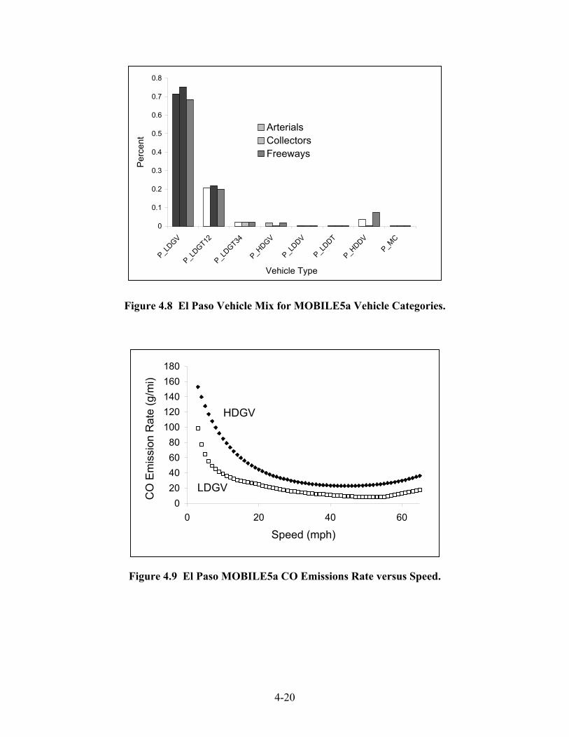
4-20

Figure 4.8 El Paso Vehicle Mix for MOBILE5a Vehicle Categories.

Figure 4.9 El Paso MOBILE5a CO Emissions Rate versus Speed.

020406080

100120140160180

0 20 40 60

Speed (mph)

CO

Em

issi

on R

ate

(g/m

i)

HDGV

LDGV

0

0.1

0.2

0.3

0.4

0.5

0.6

0.7

0.8

P_LDGV

P_LDGT12

P_LDGT34

P_HDGV

P_LDDV

P_LDDT

P_HDDV

P_MC

Vehicle Type

Per

cent

ArterialsCollectorsFreeways

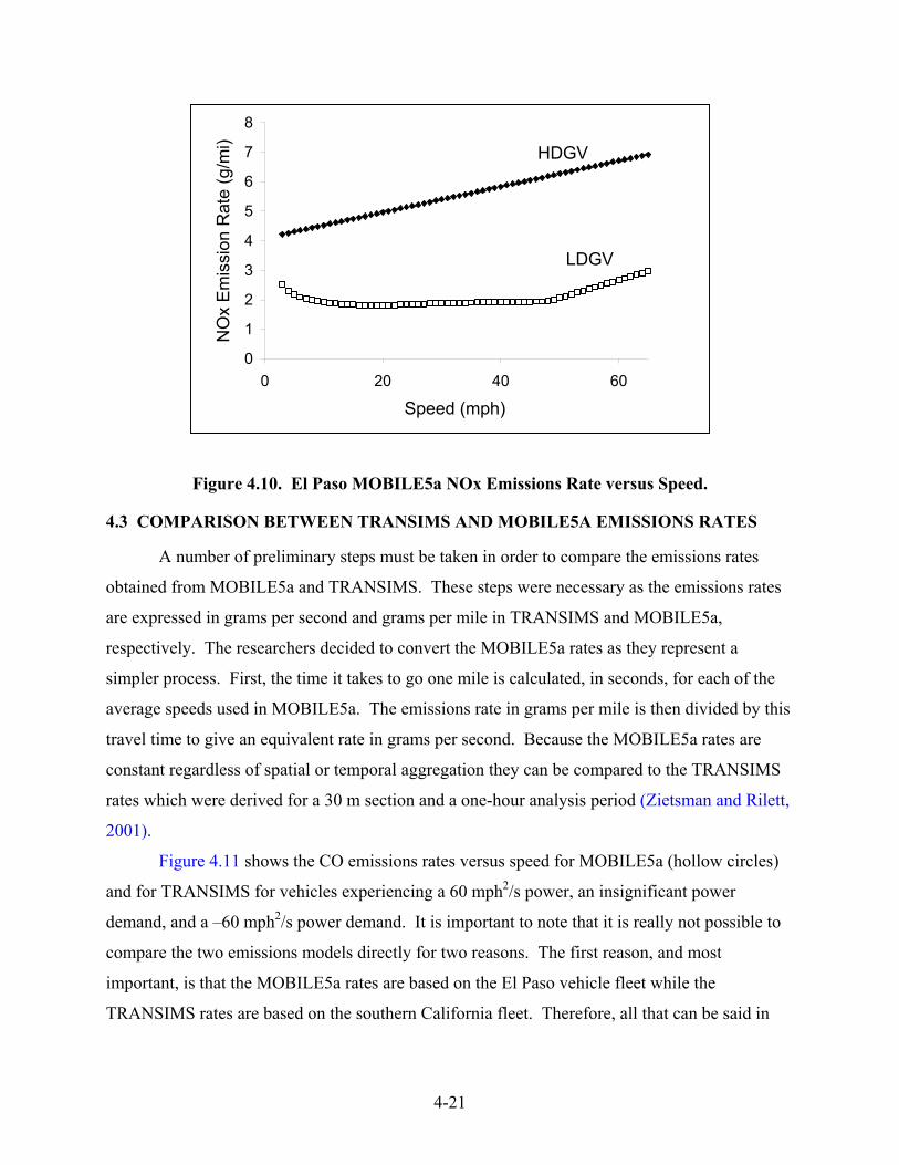
4-21

Figure 4.10. El Paso MOBILE5a NOx Emissions Rate versus Speed.

4.3 COMPARISON BETWEEN TRANSIMS AND MOBILE5A EMISSIONS RATES

A number of preliminary steps must be taken in order to compare the emissions rates

obtained from MOBILE5a and TRANSIMS. These steps were necessary as the emissions rates

are expressed in grams per second and grams per mile in TRANSIMS and MOBILE5a,

respectively. The researchers decided to convert the MOBILE5a rates as they represent a

simpler process. First, the time it takes to go one mile is calculated, in seconds, for each of the

average speeds used in MOBILE5a. The emissions rate in grams per mile is then divided by this

travel time to give an equivalent rate in grams per second. Because the MOBILE5a rates are

constant regardless of spatial or temporal aggregation they can be compared to the TRANSIMS

rates which were derived for a 30 m section and a one-hour analysis period (Zietsman and Rilett,

2001).

Figure 4.11 shows the CO emissions rates versus speed for MOBILE5a (hollow circles)

and for TRANSIMS for vehicles experiencing a 60 mph2/s power, an insignificant power

demand, and a –60 mph2/s power demand. It is important to note that it is really not possible to

compare the two emissions models directly for two reasons. The first reason, and most

important, is that the MOBILE5a rates are based on the El Paso vehicle fleet while the

TRANSIMS rates are based on the southern California fleet. Therefore, all that can be said in

0

1

2

3

4

5

6

7

8

0 20 40 60

Speed (mph)

NO

x E

mis

sion

Rat

e (g

/mi) HDGV

LDGV

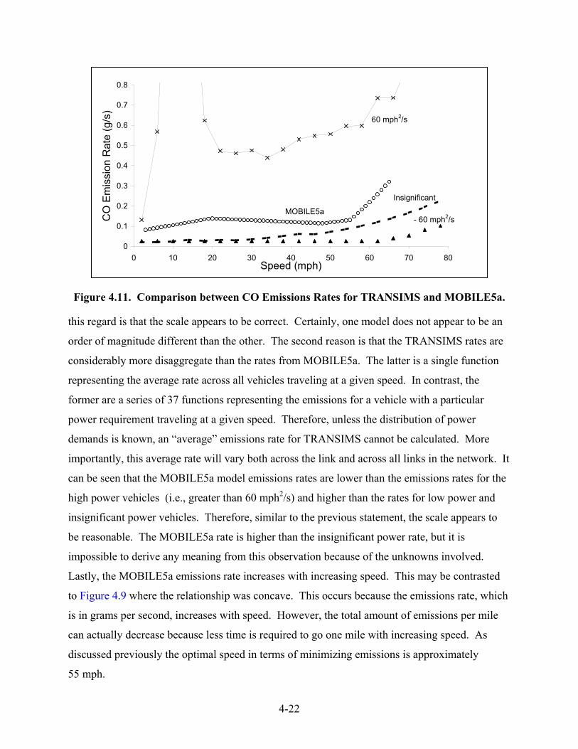
4-22

Figure 4.11. Comparison between CO Emissions Rates for TRANSIMS and MOBILE5a.

this regard is that the scale appears to be correct. Certainly, one model does not appear to be an

order of magnitude different than the other. The second reason is that the TRANSIMS rates are

considerably more disaggregate than the rates from MOBILE5a. The latter is a single function

representing the average rate across all vehicles traveling at a given speed. In contrast, the

former are a series of 37 functions representing the emissions for a vehicle with a particular

power requirement traveling at a given speed. Therefore, unless the distribution of power

demands is known, an “average” emissions rate for TRANSIMS cannot be calculated. More

importantly, this average rate will vary both across the link and across all links in the network. It

can be seen that the MOBILE5a model emissions rates are lower than the emissions rates for the

high power vehicles (i.e., greater than 60 mph2/s) and higher than the rates for low power and

insignificant power vehicles. Therefore, similar to the previous statement, the scale appears to

be reasonable. The MOBILE5a rate is higher than the insignificant power rate, but it is

impossible to derive any meaning from this observation because of the unknowns involved.

Lastly, the MOBILE5a emissions rate increases with increasing speed. This may be contrasted

to Figure 4.9 where the relationship was concave. This occurs because the emissions rate, which

is in grams per second, increases with speed. However, the total amount of emissions per mile

can actually decrease because less time is required to go one mile with increasing speed. As

discussed previously the optimal speed in terms of minimizing emissions is approximately

55 mph.

0

0.1

0.2

0.3

0.4

0.5

0.6

0.7

0.8

0 10 20 30 40 50 60 70 80Speed (mph)

CO

Em

issi

on R

ate

(g/s

)60 mph2/s

- 60 mph2/s

Insignificant

MOBILE5a

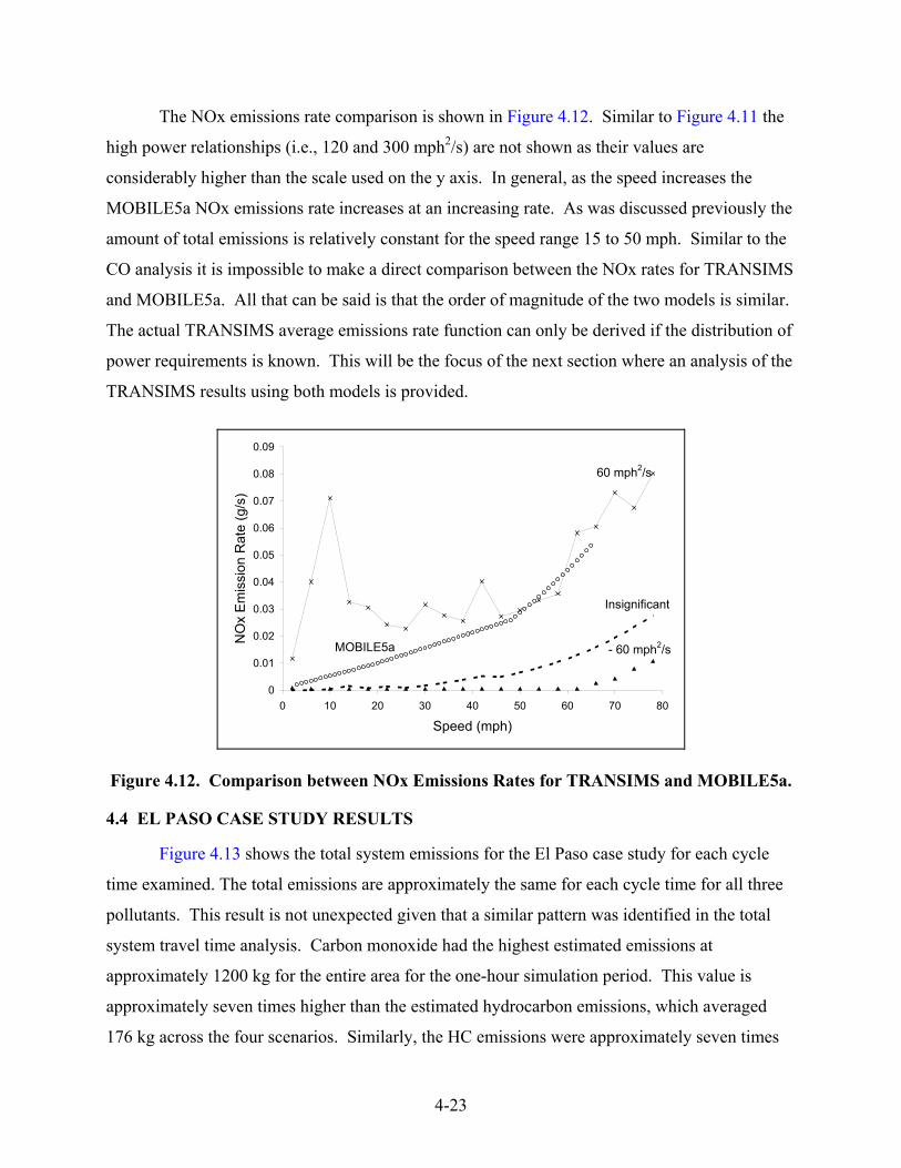
4-23

The NOx emissions rate comparison is shown in Figure 4.12. Similar to Figure 4.11 the

high power relationships (i.e., 120 and 300 mph2/s) are not shown as their values are

considerably higher than the scale used on the y axis. In general, as the speed increases the

MOBILE5a NOx emissions rate increases at an increasing rate. As was discussed previously the

amount of total emissions is relatively constant for the speed range 15 to 50 mph. Similar to the

CO analysis it is impossible to make a direct comparison between the NOx rates for TRANSIMS

and MOBILE5a. All that can be said is that the order of magnitude of the two models is similar.

The actual TRANSIMS average emissions rate function can only be derived if the distribution of

power requirements is known. This will be the focus of the next section where an analysis of the

TRANSIMS results using both models is provided.

0

0.01

0.02

0.03

0.04

0.05

0.06

0.07

0.08

0.09

0 10 20 30 40 50 60 70 80

Speed (mph)

NO

x E

mis

sion

Rat

e (g

/s)

60 mph2/s

- 60 mph2/s

Insignificant

MOBILE5a

Figure 4.12. Comparison between NOx Emissions Rates for TRANSIMS and MOBILE5a.

4.4 EL PASO CASE STUDY RESULTS

Figure 4.13 shows the total system emissions for the El Paso case study for each cycle

time examined. The total emissions are approximately the same for each cycle time for all three

pollutants. This result is not unexpected given that a similar pattern was identified in the total

system travel time analysis. Carbon monoxide had the highest estimated emissions at

approximately 1200 kg for the entire area for the one-hour simulation period. This value is

approximately seven times higher than the estimated hydrocarbon emissions, which averaged

176 kg across the four scenarios. Similarly, the HC emissions were approximately seven times

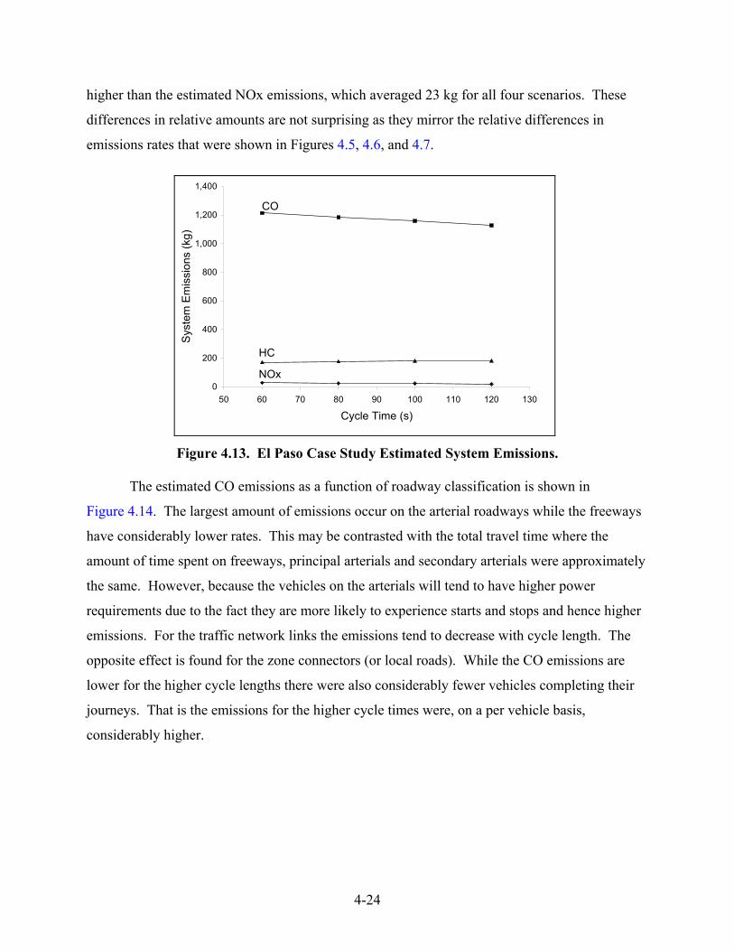
4-24

higher than the estimated NOx emissions, which averaged 23 kg for all four scenarios. These

differences in relative amounts are not surprising as they mirror the relative differences in

emissions rates that were shown in Figures 4.5, 4.6, and 4.7.

0

200

400

600

800

1,000

1,200

1,400

50 60 70 80 90 100 110 120 130

Cycle Time (s)

Sys

tem

Em

issi

ons

(kg)

HC

NOx

CO

Figure 4.13. El Paso Case Study Estimated System Emissions.

The estimated CO emissions as a function of roadway classification is shown in

Figure 4.14. The largest amount of emissions occur on the arterial roadways while the freeways

have considerably lower rates. This may be contrasted with the total travel time where the

amount of time spent on freeways, principal arterials and secondary arterials were approximately

the same. However, because the vehicles on the arterials will tend to have higher power

requirements due to the fact they are more likely to experience starts and stops and hence higher

emissions. For the traffic network links the emissions tend to decrease with cycle length. The

opposite effect is found for the zone connectors (or local roads). While the CO emissions are

lower for the higher cycle lengths there were also considerably fewer vehicles completing their

journeys. That is the emissions for the higher cycle times were, on a per vehicle basis,

considerably higher.

4-25

0

100,000

200,000

300,000

400,000

500,000

600,000

Zone C

onne

ctors

Freeway

s

Princip

al Arte

rials

Secon

dary

Arteria

ls

Collec

tors

Other

Functional Classification

CO

Em

issi

ons

(g)

6080100120

Cycle Time (s)

Figure 4.14. Estimated CO Emissions by Functional Classification.

Figure 4.15 shows the NOx emissions as a function of roadway classification. There is a

similar relationship to that of the CO emissions. However, it should be noted that the relative

differences, across road types and across cycle times, are more pronounced. The similarity in

pattern between the HC and NOx results should not be surprising because their respective

emissions rate functions, shown in Figures 4.5 and 4.6, also had similar shapes.

0

2,000

4,000

6,000

8,000

10,000

12,000

Zone C

onne

ctors

Freeway

s

Princip

al Arte

rials

Secon

dary

Arteria

ls

Collec

tors

Other

Functional Classification

NO

x E

mis

sion

s (g

) 6080100120

Cycle Time (s)

Figure 4.15. Estimated NOx Emissions by Functional Classification.

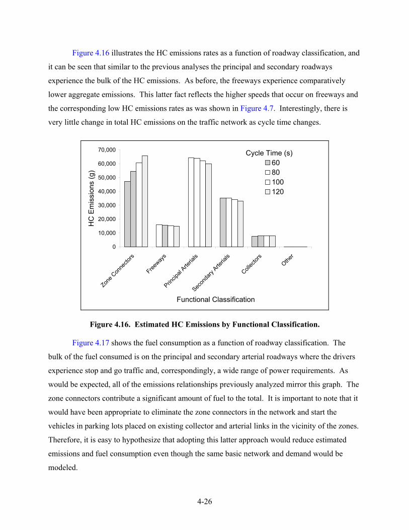
4-26

Figure 4.16 illustrates the HC emissions rates as a function of roadway classification, and

it can be seen that similar to the previous analyses the principal and secondary roadways

experience the bulk of the HC emissions. As before, the freeways experience comparatively

lower aggregate emissions. This latter fact reflects the higher speeds that occur on freeways and

the corresponding low HC emissions rates as was shown in Figure 4.7. Interestingly, there is

very little change in total HC emissions on the traffic network as cycle time changes.

0

10,000

20,000

30,000

40,000

50,000

60,000

70,000

Zone C

onne

ctors

Freeway

s

Princip

al Arte

rials

Secon

dary

Arteria

ls

Collec

tors

Other

Functional Classification

HC

Em

issi

ons

(g)

6080100120

Cycle Time (s)

Figure 4.16. Estimated HC Emissions by Functional Classification.

Figure 4.17 shows the fuel consumption as a function of roadway classification. The

bulk of the fuel consumed is on the principal and secondary arterial roadways where the drivers

experience stop and go traffic and, correspondingly, a wide range of power requirements. As

would be expected, all of the emissions relationships previously analyzed mirror this graph. The

zone connectors contribute a significant amount of fuel to the total. It is important to note that it

would have been appropriate to eliminate the zone connectors in the network and start the

vehicles in parking lots placed on existing collector and arterial links in the vicinity of the zones.

Therefore, it is easy to hypothesize that adopting this latter approach would reduce estimated

emissions and fuel consumption even though the same basic network and demand would be

modeled.

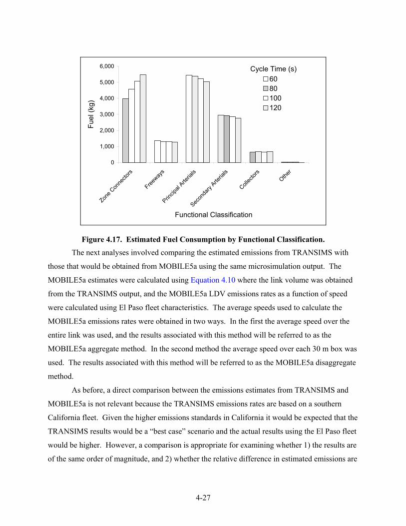
4-27

0

1,000

2,000

3,000

4,000

5,000

6,000

Zone C

onne

ctors

Freeway

s

Princip

al Arte

rials

Secon

dary

Arteria

ls

Collec

tors

Other

Functional Classification

Fuel

(kg)

6080100120

Cycle Time (s)

Figure 4.17. Estimated Fuel Consumption by Functional Classification.

The next analyses involved comparing the estimated emissions from TRANSIMS with

those that would be obtained from MOBILE5a using the same microsimulation output. The

MOBILE5a estimates were calculated using Equation 4.10 where the link volume was obtained

from the TRANSIMS output, and the MOBILE5a LDV emissions rates as a function of speed

were calculated using El Paso fleet characteristics. The average speeds used to calculate the

MOBILE5a emissions rates were obtained in two ways. In the first the average speed over the

entire link was used, and the results associated with this method will be referred to as the

MOBILE5a aggregate method. In the second method the average speed over each 30 m box was

used. The results associated with this method will be referred to as the MOBILE5a disaggregate

method.

As before, a direct comparison between the emissions estimates from TRANSIMS and

MOBILE5a is not relevant because the TRANSIMS emissions rates are based on a southern

California fleet. Given the higher emissions standards in California it would be expected that the

TRANSIMS results would be a “best case” scenario and the actual results using the El Paso fleet

would be higher. However, a comparison is appropriate for examining whether 1) the results are

of the same order of magnitude, and 2) whether the relative difference in estimated emissions are

4-28

similar across facility types. For ease of presentation all the TRANSIMS results are for a cycle

length of 60 seconds. However, similar results were found for the other three scenarios.

Figure 4.18 shows the estimated CO emissions as a function of functional classification.

There are two points to this figure. The first point is that both models had the same relative

pattern. The principal and secondary arterial roadways experienced considerably higher

emissions than the freeways even though they all experienced approximately the same total

travel time. It is hypothesized that the greater amount of accelerations and decelerations due to

traffic signals and general congestion resulted in higher emissions on these types of roadways.

The second point is that the emissions from TRANSIMS are approximately one quarter those

estimated using the MOBILE5a model. Note that the MOBILE5a CO emissions rates (in g/s)

were considerably higher than the insignificant power TRANSIMS CO emissions rates for all

speeds as was shown in Figure 4.11. It is hypothesized that there were not a lot of high power

demand vehicles modeled in the microsimulation module. If there had been the increased

emissions associated with these vehicles would have helped to minimize the difference in

emissions estimates.

0

500

1,000

1,500

2,000

2,500

Zone C

onne

ctors

Freeway

s

Princip

al Arte

rials

Secon

dary

Arteria

ls

Collec

tors

Other

Functional Classification

CO

Em

issi

ons

(kg)

TRANSIMSAggregate MOBILE5a

Figure 4.18. Comparison of Estimated CO Emissions from TRANSIMS and MOBILE5a (cycle length = 60 seconds).

4-29

The estimated NOx emissions by functional classification are shown in Figure 4.19.

There are two important points to this graph. The first is that a similar relationship to the CO

graph is obtained in that both emissions models had similar patterns with respect to roadway

classification. The second is that the difference between TRANSIMS and MOBILE5a is more

pronounced in that the former are approximately 5 to 10 percent of the latter. A difference in

estimated emissions is not unexpected because of the relatively larger difference in NOx

emissions rates between the two emissions models as was shown in Figure 4.12. Because the

relative difference in NOx emissions rates are substantially greater than the relative difference in

CO emissions rates there is a greater difference between TRANSIMS and MOBILE5a in relative

estimated emissions in Figure 4.19 as compared to Figure 4.18.

0

50

100

150

200

250

300

ZoneConnectors

Freeways PrincipalArterials

SecondaryArterials

Collectors Other

Functional Classification

NO

x E

mis

sion

s (k

g)

TRANSIMSAggregate MOBILE5a

Figure 4.19. Comparison of Estimated NOx Emissions from TRANSIMS and MOBILE5a (cycle length = 60 seconds).

A further analysis was conducted at the link level to examine differences in the emissions

models at a more disaggregate level. Figure 4.20 shows the average speed (per 30 m box) as a

function of box length for link 4607 which is a high speed primary arterial roadway. The link is

downstream from a traffic signal, and the average speed of vehicles increases as distance from

the traffic signal increases. After 120 m the average speed levels off at approximately 62 mph.

The average speeds over each 30 m box will be used as input to the MOBILE5a disaggregate

4-30

method. Also shown in Figure 4.20 is the average speed over the link which is 58 mph. The

average speed over the entire link will be used as input to the MOBILE5a aggregate method.

0

10

20

30

40

50

60

70

1 2 3 4 5 6 7 8 9 10 11 12 13 14 15 16

Box Number (box length = 30 m)

Spe

ed (m

ph)

Average Speed over Link

Figure 4.20. Speed versus Box Number for Arterial Link 4607 (cycle length = 60 seconds).

Figure 4.21 shows the CO emissions, in terms of grams emitted per 30 m block for one

hour, as a function of the box location. The first seven boxes (or 210 m) TRANSIMS estimated

the CO emissions to be approximately 6 g per box. Further down the link the emissions per box

decrease considerably. The higher upstream emissions are caused by the higher power rate, and

correspondingly higher emissions rates are associated with the vehicles accelerating to a higher

speed as was shown in Figure 4.20. There are a few CO emissions spikes (i.e., boxes 9, 11, and

14), and it is not clear why these occur given the average speed is relatively constant from

boxes 5 through 16.

4-31

0

10

20

30

40

50

60

1 2 3 4 5 6 7 8 9 10 11 12 13 14 15 16

Box Number (box length = 30 m)

CO

Em

issi

ons

(g/b

ox)

TRANSIMS

Disaggregate MOBILE5a

Aggregate MOBILE5a

Figure 4.21. CO Emissions versus Box Number for Arterial Link 4607 (cycle length = 60 seconds).

The aggregate MOBILE5a CO emissions per box are shown by a straight line as they are

constant because the average link speed is used to identify the emissions rates. Similar to the

system results the estimated CO emissions from MOBILE5a are considerably higher than those

of TRANSIMS because the relative difference in CO emissions rates between the models is

smaller at the higher speeds as was shown in Figure 4.11. The estimated aggregate CO

emissions were approximately four times greater than those estimated by TRANSIMS for this

link.

The MOBILE5a disaggregate emissions results are also shown in Figure 4.21. It can be

seen that for every box the estimated CO emissions using the disaggregate approach are higher

than those estimated using the aggregate approach. This is not unexpected because the optimal

MOBILE5a CO emissions rate occurs at approximately 58 mph as was shown in Figure 4.9.

Because the boxes all experienced lower or higher average speeds their estimated emissions

would also be higher. These results indicate the importance of defining the spatial (and

temporal) aggregation level in a consistent manner when using the MOBILE suite of models.

The aggregation issue pertains to not only TRANSIMS output, but also to 1) output from all

microsimulation models such as CORSIM and 2) output from traditional four-step models.

Because of the convex shape of the LDV emissions curves smaller aggregation intervals will

4-32

tend to result in higher estimated emissions, all else being equal. The amount of difference in the

estimated emissions will be a function of the link speed and aggregation size.

Figure 4.22 shows the NOx emissions, in terms of grams emitted per 30 m block for one

hour, as a function of the box location. Similar to the CO analysis the NOx emissions are higher

in the upstream sections than the downstream sections. It is hypothesized that this is caused by

the higher power demands required for accelerating to the higher speeds. As before boxes 9 and

11 had emissions spikes. Interestingly, box 14 had the lowest value of any section of link 4607.

While the aggregate MOBILE5a NOx emissions for this link are approximately 35 percent

higher than the aggregate TRANSIMS emissions they are of the same relative magnitude. The

MOBILE5a dissagregate method estimated emissions are also shown in this graph. On average

these are 5 percent higher than the aggregate estimated emissions. Boxes 1 through 3 had lower

emissions as compared to the aggregate approach because the emissions rates for lower speeds

are lower than that of the average link speed as shown in Figure 4.10. As before, the aggregation

size affected the MOBILE5a emissions estimates, all else being equal, because of the non-linear

relationship between emissions rate and speed.

0

1

2

3

4

5

6

7

8

1 2 3 4 5 6 7 8 9 10 11 12 13 14 15 16

Box Number (box length = 30m)

NO

x E

mis

sion

s (g

/box

)

TRANSIMSDisaggregate MOBILE5a Aggregate MOBILE5a

Figure 4.22. NOx Emissions versus Box Number for Arterial Link 4607 (cycle length = 60 seconds).

4-33

4.5 LESSONS LEARNED

There are a number of lessons identified in this chapter and these are summarized below:

1. TRANSIMS emissions are estimated using aggregated output. While the TRANSIMS traffic module simulates vehicles individually, the fidelity level chosen is not conducive to estimating emissions directly from the trajectories using disaggregate models such as CMEM. Rather aggregate output, in the form of the number of vehicles achieving one of six integer speeds over a one-hour period in each 30 m block, is output. The emissions are estimated in a two-step process. First the aggregate output is further disaggregated into 18 speed bins and 34 power levels (as defined by the acceleration speed product) based on empirically derived relationships. An emissions rate, which is based on the CMEM model, is associated with each of the 18 by 34 cells. The product of the volume and associated emissions rate for each cell is calculated, and the total is summed to give the hourly emissions per 30 m block. This estimate is subsequently adjusted using predefined multipliers that account for the fact that not all vehicles are operating with optimally warm engines.

2. There are a number of fundamental differences between MOBILE5a and the TRANSIMS emissions module. Similar to the MOBILE5a model the TRANSIMS emissions module accounts for cold start, warmth of engine, vehicle type, and so on. The fundamental difference is that the MOBILE5a suite of models only considers an average rate of emissions. This rate is not a function of spatial or temporal aggregation – that is, the rate is the same if the link length is 30 m or 300 m and is the same if the analysis time is one minute or one hour. More importantly, extreme conditions, when the engine can transition to an enrichment phase and where the emissions are significantly higher, are explicitly considered in TRANSIMS. While a direct comparison of the emissions rates was impossible because of different fleet compositions, the order of magnitude of the emissions rates are similar.

3. It is currently impossible to state definitively that TRANSIMS will have higher or lower emissions estimates than the MOBILE5 suite of models. There are many factors that effect the TRANSIMS emissions estimates including fleet type, power requirements, traffic signal settings, and so forth. Consequently, it is impossible to state a priori whether the rates will be higher or lower for a given situation. It is possible to hypothesize that in highly congested networks where there is significant stopping and accelerating that TRANSIMS will estimate higher emissions as compared to networks that have low levels of congestion. This is because it explicitly accounts for excessive emissions associated with these maneuvers.

It was found that TRANSIMS estimated considerably lower emissions for both CO and NOx as compared to MOBILE5a using the same microsimulation data as input. This result reflected 1) that the MOBILE5a emissions rates are higher than TRANSIMS emissions rates for “insignificant” power requirements, 2) that the El Paso microsimulation results did not have a large number of vehicles experiencing high power requirements (which would have increased the TRANSIMS estimated emissions), and 3)

4-34

the fact that the TRANSIMS emissions rates were based on southern California data while the MOBILE5a rates were based on El Paso data.

5-1

REFERENCES

1. Barth, M., T. Younglove, T. Wenzel, G. Scora, F. An, M. Ross, and J. Norbeck. “Analysis of Modal Emissions for a Diverse In-Use Vehicle Fleet,” Transportation Research Record 1587, TRB, National Research Council, Washington, D.C., 1997, pp. 73-84.

2. Beckman, Richard J., Keith A. Baggerley, and Michael D. McKay. “Creating Synthetic

Baseline Populations,” Transportation Research A, 30, Number 6, pp. 415-429. 3. Boyce, D.E., M.R. Lupa and Y.F. Zhang. “Introducing “Feedback Into the Four-Step

Travel Forecasting Procedure versus Equilibrium Solution of a Combined Model,” Transportation Research Record 1443, TRB, National Research Council, Washington, D.C., 1994, pp. 64-74.

4. Cottrell, W.D., “Comparisons of Vehicular Emissions in Free-Flow and Congestion

Using MOBILE 4 and Highway Performance Monitoring System” Transportation Research Record 1366, Transportation Research Board, National Research Council, Washington, D. C., 1992, pp. 75-82.

5. Dresser, G. and T. Williams. “Texas TRANPLAN Applications Guide 1995”, Research

Report 974-10F, TX94/947-10F, Texas Transportation Institute, The Texas A&M University System, College Station, TX, 1995.

6. Effa, Robert C. and Lawrence C. Larson. “Development of Real-World Driving Cycles

for Estimating Facility-Specific Emissions from Light-Duty Vehicles,” Specialty Conference on the Emission Inventory: Perception and Reality, AWMA, Pasadena, California, October 18- 20, 1993.

7. Federal Highway Administration, Travel Model Improvement Program (TMIP).

“TRANSIMS—The Dallas Case Study,” FHWA-PD-99-006 HEP-22/12-98(1.5M)QE, January 1998.

8. Highway Research Board, Highway Capacity Manual, National Research Council,

Washington, D.C., 1950. 9. Jordan, D. C. Measures of Responsibility for Pollution and their Application in Road

Pricing. Master of Science Thesis, University of Alberta, Canada, 1996. 10. Levinson, David and Ajay Kumar. “Integrating Feedback into Transportation Model:

Structure and Application,” Transportation Research Record 1413, TRB, National Research Council, Washington, D.C., 1994, pp. 70-77.

11. Los Alamos National Laboratory, “TRANSIMS User Notebook: Version 1.0”, Los

Alamos National Laboratory, Report LA-UR-98-848, April 1998.

5-2

12. Nagel, K., P. Stretz, M. Pieck, S. Lecky, R. Donnelly, and C.L. Barrett. “TRANSIMS Traffic Flow Characteristics,” Los Alamos National Laboratory, Report LA-UR-97-3530, July 1997.

13. Ortuzar, J. and L. Willumsen, Modelling Transport, 2nd Edition, John Wiley and Sons,

1994. 14. Rilett, L.R. and K. Kim. “A Comparison of the TRANSIMS and CORSIM Traffic Signal

Simulation Modules,” Transportation Research Record, TRB, National Research Council, Washington, D.C., Accepted for Publication.

15. Rilett, L.R., K. Kim and B. Raney. “A Comparison of the Low Fidelity TRANSIMS and

High Fidelity CORSIM Highway Simulation Models using ITS Data,” Transportation Research Record 1739, TRB, National Research Council, Washington, D.C., 2000, pp. 1-8.

16. Rilett, LR and K-O Kim. “Comparison of TRANSIMS and CORSIM Traffic Signal

Simulation Modules,” Transportation Research Record 1748, TRB, National Research Council, Washington, D.C., 2001, pp. 18-25.

17. Smith, J.P., S. Eubank, K. Campbell, B.W. Bush, M.V. Marathe, R.J. Beckman, and C.L.

Barrett. “Feedback Research: Information Flow in TRANSIMS,” presented at the Transportation Research Board 79th Annual Meeting, Washington, DC, 12 January 2000.

18. Transportation Research Board, Highway Capacity Manual, Special Report 290, National

Research Council, Washington, D.C., 2000. 19. U.S. Department of Commerce, Bureau of Public Roads, Traffic Assignment Manual,

1964. 20. Weiner, Ed and Fred Ducca. “Upgrading Travel Demand Forecasting Capabilities,” ITE

Journal, Volume 69, Number 7, July 1999, pp. 28-33. 21. Williams, M.D., G. Thayer, M.J. Barth, and L.L. Smith. “The TRANSIMS Approach to

Emissions Estimation,” Los Alamos National Laboratory, LA-UR 99-471, 1999. 22. Williams, M.D., G. Thayer, and L.L. Smith. “A Comparison of Emissions Estimated in

the TRANSIMS approach with those Estimated from Continuous Speeds and Accelerations,” Los Alamos National Laboratory, LA-UR 98-3162, 1998.

23. United States Environmental Protection Agency (U.S. EPA). “Federal Test Procedure

Review Project: Preliminary Technical Report,” EPA 420-R-93-007, Office of Air and Radiation, Washington, D.C., 1993.

24. United States Environmental Protection Agency (U.S. EPA) , http://www.epa.gov/.

Washington, D.C., accessed January 2001.

5-3

25. Zietsman, J. and L.R. Rilett. “Analysis of Aggregation Effects in Vehicular Emission

Estimation,” Transportation Research Record 1750, TRB, National Research Council, Washington, D.C., 2001, pp. 56-63.