Eight-year Climatology of Dust Optical Depth on Mars

L. Montabonea,b,c,∗, F. Forgeta, E. Milloura, R. J. Wilsond, S. R. Lewise,B. A. Cantorf, D. Kassg, A. Kleinbohlg, M. T. Lemmonh, M. D. Smithi,

M. J. Wolffj

aLaboratoire de Meteorologie Dynamique, Universite Pierre et Marie Curie, Paris,France.

bDepartment of Physics, University of Oxford, Oxford, UK.cSpace Science Institute, Boulder, CO, USA.

dGFDL, Princeton, NJ, USA.eDepartment of Physical Sciences, The Open University, UK.

fMalin Space Science Systems, San Diego, CA, USA.gJPL, Pasadena, CA, USA.

hTexas A&M University, College Station, TX, USA.iNASA Goddard Space Flight Center, Greenbelt, MD, USA.

jSpace Science Institute, Boulder, CO, USA.

Abstract

We have produced a multiannual climatology of airborne dust from Martianyear 24 to 31 using multiple datasets of retrieved or estimated column opticaldepths. The datasets are based on observations of the Martian atmospherefrom April 1999 to July 2013 made by different orbiting instruments: theThermal Emission Spectrometer (TES) aboard Mars Global Surveyor, theThermal Emission Imaging System (THEMIS) aboard Mars Odyssey, and theMars Climate Sounder (MCS) aboard Mars Reconnaissance Orbiter (MRO).The procedure we have adopted consists of gridding the available retrievals ofcolumn dust optical depth (CDOD) from TES and THEMIS nadir observa-tions, as well as the estimates of this quantity from MCS limb observations.Our gridding method calculates averages on a regularly spaced, but possiblyincomplete, spatio-temporal grid, using an iterative procedure weighted inspace, time, and retrieval uncertainty. In order to evaluate strengths andweaknesses of the resulting gridded maps, we associate values of weighted

∗Laboratoire de Meteorologie Dynamique, Universite Pierre et Marie Curie, Tour 45-55,3eme etage, 4, place Jussieu, 75252 Paris Cedex 05, France.

Email address: lmontabone@SpaceScience.org (L. Montabone)

Preprint submitted to Icarus August 18, 2018

arX

iv:1

409.

4841

v1 [

astr

o-ph

.EP]

17

Sep

2014

standard deviation with every grid point average, and compare with indepen-dent observations of CDOD by PanCam cameras and Mini-TES spectrome-ters aboard the Mars Exploration Rovers (“Spirit” and “Opportunity”), aswell as the Compact Reconnaissance Imaging Spectrometer for Mars aboardMRO. We have statistically analyzed the irregularly gridded maps to providean overview of the dust climatology on Mars over eight years, specifically inrelation to its interseasonal and interannual variability. Finally, we have pro-duced multiannual, regular daily maps of CDOD by spatially interpolatingthe irregularly gridded maps using a kriging method. These synoptic mapsare used as dust scenarios in the Mars Climate Database version 5, and areuseful in many modelling applications in addition to forming a basis for in-strument intercomparisons. The derived dust maps for the eight availableMartian years (currently version 1.5) are publicly available and distributedwith open access.

Keywords: Mars, atmosphere, Martian dust, Dust climatology, Martiandust storms

1. Introduction

The dust cycle is currently considered as the key process controllingthe variability of the Martian climate at interseasonal and interannual timescales, as well as the weather variability at much shorter time scales. Theatmospheric thermal and dynamical structures, as well as the transport ofaerosols and chemical species, are all strongly dependent on the dust spatio-temporal distribution, particle sizes, and optical properties.

Since the first scientific observations of a planet-encircling dust stormby ground-based telescopes in the late 50’s, dust has been one of the mainobjectives of many of the spacecraft missions to Mars over more than 40years. Recent and ongoing missions, such as Mars Global Surveyor (MGS),Mars Odyssey (ODY), Mars Express, Mars Exploration Rover (MER), MarsReconnaissance Orbiter (MRO), and Mars Science Laboratory, have includedspectrometers, radiometers or imagers to measure radiances at wavelengthssensitive to dust.

Atmospheric dust can be qualitatively observed by spacecraft cameras,such as the Mars Orbiter Camera (MOC) aboard MGS, and the Mars ColorImager (MARCI) aboard MRO (See Cantor et al., 2001; Cantor, 2007, 2008;Wang and Richardson, 2013, for dust climatologies based on camera observa-

2

tions, as well as the Mars Daily Weather websites1). One of the key physicalparameters used to quantify the presence of mineral dust in the atmosphereis the column (or total) optical depth (or optical thickness). It is a measure ofthe fraction of radiation at a specific wavelength that would be removed fromthe vertical component of a beam during its path through the atmosphereby absorption and scattering due to airborne dust. It can also be definedas the integral over an atmospheric column of the profile of the extinctionopacity (or extinction coefficient), where extinction accounts for absorptionand scattering.

The column optical depth is the product of dust retrievals when the ra-diances are obtained by nadir-viewing instruments. Profiles of extinctionopacity can be derived from radiances measured by limb-viewing instru-ments, providing important information on the vertical extension of the dust.Other important properties related to dust, such as the size distribution andthe optical parameters, are more difficult to retrieve from direct measure-ments of radiances (Clancy et al., 2003; Wolff and Clancy, 2003; Wolff et al.,2006, 2009). The knowledge of the spatio-temporal distribution of dust is ofprimary importance to produce quantitative estimates of dust mass mixingratios, and calculate the atmospheric heating rates due to absorption andscattering of solar and infrared (IR) radiation by airborne particles. Thesecalculations are the basis for describing the thermal forcing in Mars atmo-spheric models, and producing accurate predictions of the atmospheric state.

The choice of scenarios (i.e. spatio-temporal distributions) of dust opticaldepth has a significant impact on Martian global climate model (GCM) sim-ulations. Model studies have often been carried out with analytical specifica-tions of dust distributions, both in the horizontal and in the vertical (Forgetet al., 1999; Montmessin et al, 2004; Kuroda et al., 2008). More recently,modeling groups have been carrying out simulations with more realistic hor-izontal dust distributions, tied to TES observations (Guzewich et al., 2013a;Wang and Richardson, 2013; Kavulich et al., 2013). We propose in this pa-per to create a well-documented set of dust scenarios to be used in modelexperiments. Although we focus our attention on the column-integrated dustdistribution, it should be noted that the spatial variation of the vertical dis-tribution of dust also plays a significant role in thermal response (see e.g.

1http://www.msss.com/mars images/moc/weather reports/ for MOC,http://www.msss.com/msss images/latest weather.html for MARCI.

3

Guzewich et al., 2013a). There are a number of approaches to represent thisvertical structure, which is beyond the scope of this paper.

To date, there exist several datasets of retrieved column dust optical depth(CDOD) for Mars, spanning more than 20 Martian years (MY) since theMariner era. These datasets are highly heterogeneous, as they have been cre-ated using data from different instruments having different geometric views,spatial and temporal coverage, as well as different observing wavelengths.Nonetheless, we show in this paper that at least some of these datasets canbe appropriately used to quantitatively reconstruct the recent dust clima-tology on Mars, and characterize the variability over many seasonal cycles.This paper seeks to produce a continuous, multiannual climatology of CDODfrom early March 1999 (solar longitude Ls ∼ 104◦ in MY 24) to the end ofJuly 2013 (Ls = 360◦ in MY 31). During this period of time, the Ther-mal Emission Spectrometer (TES, Christensen et al., 2001) aboard MGS,the Thermal Emission Imaging System (THEMIS, Christensen et al., 2004)on ODY, and the Mars Climate Sounder (MCS, McCleese et al., 2007) onMRO provided global coverage of radiance observations at IR wavelengths,from which Smith et al. (2003); Smith (2004, 2009); Kleinbohl et al. (2009)obtained direct retrievals of CDOD or estimates of this quantity from theintegrated extinction profiles.

While images from orbiting spacecraft can provide information over largeareas on the planet at any given time, observations of IR radiances fromorbiting instruments have a very discrete coverage in longitude and localtime due to the choice of orbit geometry. MGS and MRO, for instance, havesun-synchronous, nearly 2-hour polar orbits, which provide good latitudecoverage but only sample about a dozen longitudes, usually at close to twofixed local times of day except when crossing the poles (dust can often only beretrieved in the daytime, restricting further to one local time). Because duststorms on Mars have a wide range of spatial and temporal scales (Cantor,2007; Wang et al., 2003, 2005), these discrete observations can affect thespace-time representation of dust storm activity. Extrapolating the datacollected along orbit tracks to a broader range of local time and longitudeintroduces even more biases. Synoptic maps produced using simple averagebinning may alter the representation of rapidly evolving dust distribution.

We have developed a gridding methodology that is specifically adapted toheterogeneous observations, and to the discrete longitudinal/temporal cover-age typical of spacecraft data acquisition. The objective is to produce daily,regularly gridded maps of absorption CDOD at 9.3 µm for several consec-

4

utive Martian years (dust opacity in absorption is less dependent on theparticle size than in extinction). To achieve the goal, we have adopted a two-step procedure. The first step consists in calculating iteratively averages andstandard deviations of observations on a regularly spaced but likely incom-plete spatio-temporal grid, after having binned the data using time windowsof different size, and applied appropriate weighting functions in space, time,and retrieval uncertainty at each iteration. We have established acceptancecriteria for the gridded values, based on the number of reliable observationsin each bin. We have used this first product to statistically study the dustvariability over almost eight complete Martian years. The second step con-sists in producing regular, daily maps of CDOD by spatially interpolatingand/or extrapolating the irregularly gridded maps, using a kriging method(see e.g. Journel and Huijbregts, 1978, for a general introduction on the tech-nique). This multiannual series of synoptic maps of CDOD is used for thedust scenarios in the GCM simulations that produce the current version ofthe Mars Climate Database (MCD version 5.1, Millour et al., 2014).

We provide open access to both the irregularly gridded and regularlykriged datasets, to foster scientific analyses and applications of the long-term Martian dust climatology. The most up-to-date version of these prod-ucts (currently v1.5) can be downloaded in the form of NetCDF files fromthe MCD project website2, hosted by the Laboratoire de Meteorologie Dy-namique (LMD). We also provide atlases of these maps as supplementarymaterial of this publication.

The outline of this paper is the following. Section 2 describes the instru-ments and data we have used to produce the dust climatology. We providedetails of the time coverage, data quality control, processing, and uncertain-ties for each instrument. In Section 3 we introduce the iterative weightedbinning methodology we have adopted to create irregularly gridded (but reg-ularly spaced) CDOD maps from the spacecraft observations. Section 4 isdevoted to discuss the internal validation of the gridded maps, as well as thevalidation with independent observations. We report in Section 5 the sta-tistical analysis of the dust climatology, in relation to the intraseasonal andinterannual variabilities. In Section 6 we discuss the assumptions we havemade and the kriging technique we have applied, with the purpose of pro-ducing regular and complete maps to be used as dust scenarios. A summary

2The URL to access the website is: http://www-mars.lmd.jussieu.fr/

5

is outlined in Section 7, including a discussion on future developments.

2. Spacecraft, instruments and observations

Mars Global Surveyor started its science mapping phase in March 1999(Ls ∼ 104◦, MY 24), after a lengthy period of aerobraking. Only about sixmonths of global observations are available in MY 23 during the aerobraking,when the spacecraft orbit was still very elliptical (6 hour orbit instead of thenominal 2 hour mapping phase orbit). MGS stopped working properly inNovember 2006, and the mission was officially ended in January 2007.

Mars Odyssey started its mapping phase in February 2002 (Ls ∼ 330◦,MY 25) and is still working at the time of writing. It is the longest runningspacecraft orbiting an extra-terrestrial planet to date.

Mars Reconnaissance Orbiter started its mapping phase in November2006 (Ls ∼ 128◦, MY 28) and, although it encountered a few problems thatkept it in safe mode for an extended period at the end of 2009, is currentlyoperating nominally.

The Mars Exploration Rovers “Spirit” and “Opportunity” started theirmissions on Mars respectively on 4th January 2004 and 25th January 2004(Ls ∼ 328◦ and Ls ∼ 339◦, MY 26). Spirit ceased communications withEarth in March 2010 (Ls ∼ 67◦, MY 30), whereas Opportunity is still activeon the surface of the planet.

For building the dust climatology described in this paper, we have usedCDOD retrievals and estimates obtained from the following instruments ob-serving at IR wavelengths:

• TES aboard MGS, from Ls = 103.6◦ in MY 24 to Ls = 82.5◦ in MY 27.After this date, the number and quality of TES observations rapidlydecreased (August 2004). CDOD retrievals (Smith, 2004) are in absorp-tion (scattering is not modeled) from nadir observations at wavelengthscentered around 1075 cm−1 (9.3 µm). Local times are narrowly cen-tered around 2pm at most latitudes, except when the orbit crosses highlatitudes.

• THEMIS aboard ODY, from Ls = 0◦ in MY 26 (we did not use ob-servations taken at the end of MY 25) to Ls = 360◦ in MY 31. Theinstrument is still working at the time of writing. CDOD retrievals(Smith et al., 2003; Smith, 2009) are in absorption from nadir observa-tions at wavelengths centered around 1075 cm−1 (9.3 µm) as for TES.

6

Local times are between 2.30pm and 6pm at most equatorial and mid-latitudes (except for latitudes polewards of |60◦|).

• MCS aboard MRO, from Ls = 111.3◦ in MY 28 to Ls = 360◦ in MY 31.MCS was switched on in September 2006 before the official beginningof MRO primary science phase, but had a long period in MY 28 (be-tween 9th February and 14th June 2007) during which a mechanicalproblem preventing the use of its elevation actuator forced the teamto keep it in limb-staring mode. The event precluded any nadir oroff-nadir observation during this period, with the effect of limiting thevertical extension of the retrieved profiles (including those of extinctionopacity) in the lower part of the atmosphere. Since 9th October 2007,off-nadir measurements with surface incidence angles between about60◦ and 70◦ have resumed with nearly every limb sequence, but forretrievals of aerosol extinction opacities only limb views are currentlyused. Kleinbohl et al. (2009) obtained profiles of dust extinction opac-ity from limb observations at wavelengths centered around 463 cm−1

(21.6 µm) as standard MCS product. In this paper we have used esti-mates of CDOD from the limb observations, as detailed in Section 2.1.2.Local times are centered around 3am and 3pm at most latitudes, ex-cept when the orbit crosses the polar region. Since 13th September2010 (Ls = 146◦, MY 30) MCS has also been able to observe cross-track, thus providing information in a range of local times at selectedpositions during MRO orbits (Kleinbohl et al., 2013). We include thesecross-track observations in our gridding, when available.

For the validation of the gridded maps with independent observations, wehave used retrievals of near-IR and IR CDOD from the following instruments:

• PanCam cameras (Bell et al., 2003) aboard MER-A “Spirit” and MER-B “Opportunity”, respectively from Ls ∼ 328◦ and Ls ∼ 339◦ in MY 26.Spirit PanCam stopped providing measurements after Ls ∼ 67◦ inMY 30. Lemmon et al. (2014) have retrieved CDOD from upward-looking nadir observations at wavelengths centred around 880 nm (nearIR) and 440nm (visible blue). In this work we use only retrievals at 880nm. There are no significant differences between the values providedat the two wavelengths.

• Mini-TES aboard MER “Spirit” and “Opportunity” (Christensen et al.,2003), starting from the same times as PanCam cameras until Ls ∼ 191◦

7

(Spirit) and Ls ∼ 269◦ (Opportunity) in MY 28. After Ls ∼ 269◦ thedetectors were covered by dust from the MY 28 planet-encircling duststorm and became unreliable. Smith et al. (2006) have retrieved CDODfrom upward-looking nadir observations at IR wavelengths centeredaround 1075 cm−1 (9.3 µm).

• CRISM (Murchie et al., 2007) aboard MRO, from Ls ∼ 133◦ in MY 28until Ls = 360◦ in MY 30. CDOD retrievals have been obtained fromnadir observations at wavelengths centred around 900 nm (Wolff et al.,2009). Although there are CRISM observations available after Ls =360◦ in MY 30, and CRISM is still working at the time of writing, weare not using these observations in the present work because an issueof truncated EPFs in MY 31 requires further investigation.

Figure A.1 shows a summary of the time periods for which observationsfrom the above mentioned instruments are available, together with the timelimits within which we have used them in this paper.

— Figure A.1 —

In addition to CDOD data, we have also used visible wide-angle picturesfrom MGS/MOC (Malin et al., 2010), and visible pictures from MRO/MARCI(Bell et al., 2009). The main purpose is to compare the evolution of selecteddust storms in the reconstructed CDOD maps to the daily evolution thatcan be appreciated in camera images of the Martian surface.

2.1. Data quality control

Before using the CDOD datasets retrieved from the different instruments,we have firstly checked the values against quality control criteria to eliminateunreliable data.

For all datasets, negative values are only allowed if the sum of the valueand the associated uncertainty (see Section 2.3) is non-negative. Althougha single negative measurement (in this specific case a ‘measurement’ corre-sponds to a ‘retrieval’) can be considered unphysical, the weight of negativemeasurements must be taken into account in statistical calculations to pre-vent biases towards statistically non-zero values. It is anticipated that boththe gridded values described in Section 3 and the interpolated ones describedin Section 6 are only accepted if they are positive, otherwise they are replacedby a minimum positive value of 0.02.

8

For specific datasets, we have adopted the following quality control crite-ria. We show in Figures A.2 and A.3 the number of CDOD retrievals usedin the present work.

2.1.1. TES and THEMIS

For TES, we have retained CDOD observations flagged as “good quality”by the TES team, which passed additional quality control criteria. Specifi-cally, we require that the surface temperature is greater than 220 K (Smith,2004), the difference between surface temperature and maximum atmospherictemperature is greater than 5 K, the radiance fit residual is lower than 20,the opacity of the carbon dioxide hot bands is between -0.01 and 0.05, andthe water ice opacity is greater than -0.05 (the negative value threshold isconstrained by the uncertainty). The surface temperature threshold insuresa good signal-to-noise ratio, whereas the threshold on the temperature dif-ference between surface and atmosphere prevents unreliable retrievals whenthe temperature contrast is too small. The latter case is particularly validduring high dust loading conditions, as showed by results from the Geophys-ical Fluid Dynamics Laboratory GCM (GFDL-GCM) and comparison withMOC images during the 2001 planet-encircling dust storm (Wilson et al.,2011). With the choice of these quality control criteria, retrievals are practi-cally limited to daytime conditions over ice-free surfaces, and may be reducedduring intense dust storms (see Figs A.2 and A.3).

THEMIS CDOD retrievals include several “framelets” in the same “im-age”, i.e. several values within the same stripe of observations. Only thelast framelet of each image is properly calibrated, but in this study we haveconsidered all available framelets to increase the number of THEMIS obser-vations, especially in MY 27 when we use no other observations. We associatea slightly larger uncertainty to non-calibrated framelets, as explained in Sec-tion 2.3. For quality control purposes, we have retained CDOD values whenthe rms residual from the aerosol opacity fit is lower than 0.4, and the surfacetemperature is greater than 210 K.

2.1.2. MCS

MCS observes the atmosphere in limb and off-nadir modes, which has theadvantage of allowing the retrieval of vertical profiles of dust opacity, but hasthe disadvantage of not being able to observe the first few kilometres abovethe ground (depending on the angle of observation). In order to estimatethe column optical depth for aerosol dust, the MCS team has integrated the

9

full profile of dust extinction opacity produced by the retrieval algorithm(v4.0 is the version used in this work) after a successful retrieval. The pro-file is extended upward and downward under the assumption of well mixeddust, based on the last valid value. The standard retrieved dust profile isoften truncated when regions have measured radiances that are not fit bythe forward radiative model within defined thresholds in dust, water ice ortemperature. In the upper levels, the minimum extinction coefficient thresh-old for dust is 10−9 km−1. In the lower levels, the profiles can get saturatedby high opacity values, exceeding the threshold of 10−3 km−1 (Kleinbohl etal., 2009). Column optical depth estimates, on the other hand, use non-truncated profiles to make sure all available and reasonable information istaken into account. The MCS dust profiles cannot be retrieved down to thesurface, and the dust in the un-retrieved part of the profile can account for asignificant fraction of the total dust column. Estimates of CDOD from MCSobservations, therefore, are likely to introduce errors attributable to eitherthe extrapolation to the surface under the well mixed assumption or the useof dust opacity values at altitudes where the fit to observed radiances is notwithin the standard threshold. This problem may be particularly acute inlight of evidence of elevated dust layers (Heavens et al., 2011; Guzewich etal., 2013b).

MCS CDOD estimates can be fairly inaccurate if the lowest retrieved levelof dust opacity is above ∼ 20 km altitude, depending on the time of the yearand the dust/water ice conditions. We have therefore retained CDODs thatcorrespond to dust extinction profiles with valid values at least at or below25 km altitude. Dayside retrievals are particularly affected by low altitudeaereosols. To prevent large extrapolation of dust extinction coefficient tothe surface during daytime observations, we only accept estimated daytimeCDODs when the corresponding extinction profile has valid values below 8km altitude.

Furthermore, we have rejected CDOD estimates when the temperatureprofile dropped below the condensation temperature of carbon dioxide atsome pressure levels, because CO2 ice opacity can affect retrievals of dustopacity at those levels (carbon dioxide ice opacity is not currently takeninto account in MCS retrievals). It is worth mentioning that this selectionmight introduce a systematic bias, especially during the northern spring andsummer seasons in the tropics. TES provides daytime CDODs while MCSestimates of CDOD in this season are largely based on nighttime viewing,because daytime clouds in the aphelion tropical belt limit the success of

10

retrievals.

— Figure A.2 —

— Figure A.3 —

2.2. Data processing

The CDODs from TES/THEMIS and MCS are retrieved at different IRwavelengths, in absorption for TES/THEMIS and in extinction for MCS,which prevents the direct comparison. We account for this problem by con-verting the estimated MCS extinction CDODs at 21.6 µm into equivalentabsorption CDODs at 9.3 µm. We carry out the conversion by multiplyingthe MCS values by a factor 2.7, which takes into account the effective dustparticle radius (1.06 µm) and variance (0.3) used in the retrievals (version4.0, Kleinbohl et al., 2009, 2011). It is worth mentioning that the dust sizedistribution is maintained fixed throughtout all seasons and locations.

We use CDOD from PanCam cameras aboard MER-A and MER-B roversat the near-IR wavelength of 880 nm. CRISM CDOD retrievals are obtainedat the near-IR wavelength of 900 nm. When using PanCam and CRISM forvalidating the gridded maps in Section 4, we have to account for the dif-ferences between the absorption-only gridded values at 9.3 µm and the fullextinction near-IR retrievals. This is done by converting the gridded val-ues into equivalent visible values. The process firstly converts values fromabsorption-only at 9.3 µm to full-extinction values by multiplying by a factor1.3 (Smith, 2004; Wolff and Clancy, 2003), then converts the latter to meanvisible values by multiplying by a factor 2.0, consistent with 1.5- to 2.0-µmdust particles (Clancy et al., 2003; Lemmon et al., 2004; Wolff et al., 2006).Overall, the factor we use to convert from absorption-only at 9.3 µm to equiv-alent full-extinction visible is 2.6. This factor, though, is affected by largeerrors, deriving from both the conversion to extinction (Smith, 2004), andthe infrared-to-visible conversion (Lemmon et al., 2004; Wolff et al., 2006),see also Section 2.3. This is the reason why we have decided to provide ourgridded products at the original IR wavelengths, despite the advantage ofproducing equivalent visible CDOD maps for global and mesoscale atmo-spheric models, whose radiation schemes usually compute dust heating ratesbased on mean visible opacities using assumed IR/visible ratios.

In order to calculate spatial averages, we require that CDODs are normal-ized to a reference pressure level, hence eliminating the effect of topographic

11

inhomogeneities. The retrieved values are divided by the surface pressureat the appropriate location and time of year, extracted from the pres0 toolincluded in the MCD v4.3 (Millour et al., 2011), and multiplied by 610 Pa,which is our choice for the reference pressure level. The CDODs used in thepresent study, therefore, are equivalent to integrate or extrapolate the opticaldepth down to 610 Pa at all locations on the planet, under the assumption ofwell-mixed dust. See Section 2.3 for a discussion of uncertainties associatedto surface pressure.

2.3. Data uncertainties

We have estimated the uncertainty of each single CDOD value that wehave used in this work. The total uncertainty of an observation is providedas the propagation of single uncertainties detailed in this Section, for eachinstrument. The error propagation is carried out using relative errors, whichhighly simplify the formulas. The squared relative propagated error reducesto the sum of squared relative errors on each independent variable whenoperations among variables include only multiplications and divisions, as inour case.

An uncertainty that is common to all observations is associated to thevalue of the surface pressure extracted from the MCD v4.3, which is usedto extrapolate CDODs to a specific pressure level. After the correctionsfor topography and total mass of the atmosphere, which are carried outwithin the pres0 routine of the MCD, the largest sources of surface pressurevariability on Mars are the weather systems, mainly in the form of duststorms and high latitude winter baroclinic waves. In order to account forthis variability, we have extracted the day-to-day RMS of surface pressurefrom the MCD (see the MCD Detailed Design Document associated to theversion of the database described in Millour et al., 2011) to build a 5◦ solarlongitude ×5◦ latitude array. We provide an estimate of the surface pressureuncertainty associated to the specific location and season of an observationby interpolating this array.

2.3.1. TES and THEMIS

Retrievals of CDOD from TES and THEMIS observations come with anassociated nominal uncertainty, estimated by taking into account randomerrors in the instrument and calibration, as well as possible systematic errorsin the retrieval algorithms. Smith (2004) gives an estimate for the totaluncertainty in TES absorption-only IR dust optical depth for a single retrieval

12

of 0.05 or 10% of the column optical depth, whichever is larger. Smith (2009)provides this value for THEMIS absorption-only IR dust optical depth forthe calibrated framelet: 0.04 or 10% of the column optical depth, whicheveris larger.

For THEMIS observations, Smith (2009) also states that “uncertaintiesare likely somewhat higher (perhaps 20% or even higher) during the mostintense dust storms because large corrections to the temperature profile mustbe made for those observations”. It is likely that TES retrievals during highdust loading are also affected by larger uncertainties, due to the reducedsurface-atmosphere temperature contrast and uncertainty in dust size distri-bution. In order to account for this, for TES we use the nominal uncertaintyup to IR optical depth 1.0, then we increase the uncertainty to 20% up toIR optical depth 2.0, and to 30% for IR optical depths greater than 2.0. ForTHEMIS, we use the nominal uncertainty up to IR optical depth 0.5, weincrease the uncertainty to 20% up to IR optical depth 2.0, and to 30% forIR optical depths greater than 2.0.

As for the non-calibrated THEMIS framelets, we currently increase theiruncertainties by 20% (e.g. 0.06 instead of 0.05 when the CDOD value is 0.5)

2.3.2. MCS

As explained in Section 2.1, the procedure adopted to estimate CDODfrom MCS observations is likely to introduce errors, particularly when thetruncated dust profiles do not have valid values close to the surface. Esti-mating these errors is particularly difficult, as crucial information may bemissing in the atmospheric layers where the dust loading is significant. Ourestimate of the uncertainty on MCS CDODs, therefore, can only be empiri-cal. In Section 7, we mention future developments in relation to MCS CDODretrievals.

In this work, we assign an uncertainty on the basis of the altitude ofthe lowest valid level in the dust profile used for the vertical integration.The uncertainty is linearly increasing from 5% (nominal value) to 60% as afunction of this altitude, from the surface to the highest accepted level of25 km. Although this uncertainty estimate is arbitrary, it provides a way todistinguish MCS values that are likely to be biased, and to relatively evaluatethis bias. This feature is used during the gridding procedure, as detailed inSection 3.

Very small values of CDOD estimated from dust extinction profiles thatdo not have valid values below 4 km are considered spurious and substituted

13

with the minimum value of 0.01, with 10% uncertainty (i.e. 0.001).Finally, we consider that the 2.7 factor used to convert MCS extinction

CDODs at 21.6 µm to equivalent absorption CDODs at 9.3 µm is affectedby 10% uncertainty (i.e. 0.3), due to the uncertainty on the particle sizes.We take it into account in the propagation of uncertainties for MCS.

2.3.3. PanCam and Mini-TES

We have averaged CDOD retrievals from PanCam and Mini-TES obser-vations in each available sol for both MER-Spirit and MER-Opportunity. Wehave also interpolated in time to fill the gaps in the sol-averaged time seriesfor both MERs. For sol-averaged PanCam and Mini-TES CDODs, we usethe largest value between the standard deviation and the average of singlemeasurement errors as a measure of uncertainty on the daily mean. Thischoice takes into account CDOD variations with local time as well as singlemeasurement errors.

2.3.4. Digression on absorption/extinction and IR/visible conversions

As explained in Section 2.2, we have decided to work at the original TESand THEMIS absorption IR wavelength of 9.3 µm, except when comparingwith PanCam and CRISM retrievals. The conversion factors from absorptionto extinction and from IR to visible depend on the aerosol refractive indexes,which ultimately depend on the aerosol size, shape and composition, and arelikely to vary with seasons and locations. Both factors are therefore affectedby large uncertainties. Smith (2004) shows in Fig. 4a a graph of the relation-ship between effective absorption and full extinction optical depth for dustat the equator at northern autumn equinox in MY 24 (it is stated that thecurve is typical of other times and locations). For IR dust optical depthslower than 0.5, the relationship is fairly linear (τabs = τext/1.3). The depar-ture from the linear relationship at higher dust optical depth can be estimatedas −τext2/25. This estimate could be used to introduce an uncertainty on theabsorption-to-extinction factor, which increases with the optical depth. Asfor the infrared-to-visible factor, uncertainties have been estimated in a fewmeasurement campaigns, although limited in time and location. Lemmon etal. (2004) reports a value of 2.0±0.2 from MER-PanCam observations, Wolffet al. (2006) reports in Table 2 dust optical depth values from MER-PanCamand Mini-TES, which can be averaged to provide a value of 2.5± 0.6.

In Section 4, we have simply used a single factor 2.6 (1.3×2.0) throughoutthe time series to convert the gridded values to equivalent visible values,

14

without explicitly taking the uncertainty on this factor into account.

3. Gridding dust opacity observations

The process of creating uniformly-spaced data (i.e. a regular grid) fromirregularly-spaced (scattered) data is generally known as ‘gridding’. Thereexist several techniques to solve this problem, depending on the applications.A basic technique commonly adopted when dealing with orbital spacecraftobservations is ‘binning’ using space-time box averages. The original datavalues which fall in a given multi-dimensional interval (a ‘bin’) are replacedby a value representative of that interval, often the average, but the mediancan also be used to filter outliers. If the bins are uniformly distributed, theproblem of gridding the data is solved. For our purposes, the simple box-average binning is not suitable because 1) we desire to achieve the highestpossible spatio-temporal resolution for the CDOD maps, compatibly withhaving a reasonable number of observations to grid, and 2) simple box av-erages introduce temporal and spatial biases if long time intervals and/orlarge spatial boxes are used (several orbits at different times are inevitablyaveraged together).

Reconstructing the dust climatology while preserving the desired vari-ability of dust storms at short time scale and small spatial scale, therefore,requires a more sophisticated data gridding. In order to achieve this objec-tive, we have developed an efficient ‘iterative weighted binning’ methodology,described in the following Section.

3.1. The principle of iterative weighted binning (IWB)

The application of our gridding procedure is equivalent to a movingweighted average characterized by the use of successive spatio-temporal win-dows. The basic principle of the methodology is that, for a given grid pointat a given time, all observations within a defined time window and spatialrange are averaged using weights that depend on 1) the lag between thetime of each observation and the required time at the grid point, 2) the spa-tial distance between each observation location and the location of the gridpoint, and 3) the uncertainty (standard deviation) of each observation. Inthis work, we use the Mars Universal Time (MUT) of the prime meridian asabsolute time variable to which we refer both the time of observations andthe time of grid points on a synoptic map.

15

The weighted average value Y at a given time t0 and location x0 for ageneric observed variable y, which is a function of time and spatial coordi-nates, is given by:

Y (x0, t0) =

∑n=1,N

M(δxn, δtn) ·R(δtn) ·Q(σyn/yn) · yn(xn, tn)∑n=1,N

M(δxn, δtn) ·R(δtn) ·Q(σyn/yn), (1)

where n represents the index of the N observations y1, y2, . . . yN that are in-cluded in defined time window and space range (a multi-dimensional bin builtaround the time t0 and the location x0). R is the time weighting function,which determines the contribution of the nth observation according to thetime difference δtn = tn− t0 (positive for observations in the future, negativefor observations in the past). M is the distance weighting function, whichdetermines the contribution of the nth observation according to its distanceδxn = |xn − x0| from the location x0. The distance weight is also a functionof the time lag δtn so that observations at different times in the past or in thefuture with respect to t0 have different distance weights. Q is the uncertaintyweight, which determines the contribution of the nth observation accordingto its relative uncertainty (σyn is the observation standard deviation).

The particular choice for the form of the weighting functions M , R, andQ depends on the specific application. For our purpose of creating synopticmaps of CDOD using orbiting satellite observations, it is convenient to useweighting functions similar to those implemented in the analysis correctiondata assimilation scheme of the UK Meteorological Office (Lorenc et al.,1991) and in the derived Mars analysis correction data assimilation scheme(Lewis et al., 2007). In fact, Eq. 1 applied to k grid points of a regular gridcan be considered as the weighted average equivalent of the model grid pointincrement Eq. 3.18 in the analysis correction scheme of Lorenc et al. (1991),although this analogy has no formal basis.

Eq. 1 applies to observations in specifically defined time window and spacerange. Our methodology includes the iterative use of less and less restrictivetime windows and space ranges, as we explain in the next section wherewe describe the application of IWB to the problem of gridding dust opacityobservations.

3.2. Gridding with IWB: procedure

If we apply Eq. 1 to each grid point k of a pre-defined space-time grid forthe CDOD variable τ , the weighted average value T at each grid point can

16

be written as:

Tk =

∑n=1,N

Mnk(δtnk) ·R(δtnk) ·Qn · τn∑n=1,N

Mnk(δtnk) ·R(δtnk) ·Qn

, (2)

where τ1, τ2, . . . τN are the CDOD observations that are included in a specifiedtime window and distance range built around the time and location of thegrid point k. Additionally, one can define the weighted root mean squareddeviation (or weighted standard deviation) associated to the weighted averagevalue Tk as:

σTk =

√√√√√√∑

n=1,N

Mnk ·R ·Qn(τn − Tk)2∑n=1,N

Mnk ·R ·Qn

=

√√√√√√∑

n=1,N

Mnk ·R ·Qn · τ 2n∑n=1,N

Mnk ·R ·Qn

− T 2k ,

(3)We choose M to be a second-order autoregressive correlation function of

the distance dnk from observation n to grid point k and of the correlationscale S (see also Eq. 3.19 in Lorenc et al., 1991):

Mnk = (1 + dnk/S(δtnk)) exp(−dnk/S(δtnk)), (4)

where S(δtnk) is a function of the time difference between observation timeand grid point time. S is chosen to be a linearly increasing function of thisdifference, symmetric with respect to δtnk = 0, with a minimum value Sminat δtnk = 0 and a maximum value Smax at the extrema of the chosen timewindow (TW). The equation for S (defined over the range −TM/2 < δt <TM/2) is therefore provided by:

S =Smax − Smin

TW/2|δt|+ Smin. (5)

With this choice of S, observations with times closer to the time of therequested grid point have weights Mnk that decrease faster with distance (seeFig. A.4). In other words, smaller weights are assigned to distant observationswhen their time is closer to the current time. A further parameter, dcutoff ,sets the distance range on the spherical surface within which the contributionsof the observations to the average are considered. We use the haversineformula to calculate the distance between two locations on the spherical

17

planetary surface, which is numerically better conditioned for small distances(Sinnott , 1984).

R is chosen to be a decreasing quadratic function of the difference δtnkbetween observation time and grid point time (Lorenc et al., 1991), symmet-ric with respect to δtnk = 0. The equation for R (defined over the range−TM/2 < δt < TM/2) is therefore:

R =

(Rmin − 1

TW/2|δt|+ 1

)2

, (6)

where Rmin is the minimum value at the extrema of the chosen time window(see Fig. A.4 for an example with TW = 7).

Finally, Q is chosen as a second-order autoregressive correlation functionof the relative uncertainty of observation, namely:

Qn =

(1 + λ

στnτn

)exp

(−λστn

τn

), (7)

where στn is the uncertainty (standard deviation) of each observation, and λis a scaling factor used to obtain the desired width at half maximum (WHM)for the Q function. We choose λ = 8.39173 to have WHM=0.2 (i.e. Q = 0.5when the relative uncertainty of an observation is 20%). See Fig. A.4 for aplot of the Q function we use.

— Figure A.4 —

The following is a summary of our gridding procedure with IWB.

1. We have tested the sensitivity of the method to different spatial andtemporal resolutions and the results are reported in Section 3.3. Onthe basis of the sensitivity tests, we have chosen the resolutions of thelongitude-latitude grids reported in Table A.1, according to differentdatasets. The choice of the time resolution is one sol. Each synopticgridded map is centred around local time noon at the prime meridian,i.e. a sol at 0◦ longitude is defined between 00:00 and 24:00 MUT.

2. For MY 24 and 25 we have used only TES CDODs. For MY 26 and27 we have used both TES and THEMIS observations until Ls ∼ 80◦

in MY 27, then only THEMIS observations. For MY 28, we have usedonly THEMIS until Ls ∼ 112◦, then both MCS and THEMIS, as wellas in most of MY 29, 30, and 31, apart from Ls ∼ 327◦, MY 29, toLs ∼ 24◦, MY 30, when only THEMIS observations are available.

18

3. For each set of observations (TES, TES+THEMIS, THEMIS, MCS+THEMIS)we have defined the parameters required by Eq. 2, which are summa-rized in Table A.1. The IWB procedure then requires that, for eachsol and for each spatial grid point, we define a time window and dis-tance range within which we use observations to calculate the weightedaverage and its associated weighted standard deviation.

4. We repeat the previous step iteratively, using different time windows,from the smallest to the largest (the values we use are reported inTable A.1), and calculating the weights accordingly. At each iteration,more valid grid points are added to the synoptic map, because moreobservations are considered, but we do not overwrite grid points flaggedas valid in previous iterations.

5. The criterion to accept a value of weighted average at a particular gridpoint is that there must be at least a minimum number of observationsNthr within a distance dthr from the grid point, having relative uncer-tainties lower than a threshold value (στ/τ)thr (see values in Table A.1).If this is not the case, a missing value is assigned to the grid point atthat iteration.

6. The final result of the successive application of the weighted binningequation consists in daily synoptic maps of CDOD on the pre-definedregular grid, with missing values in places where the gridding criterionwas not satisfied at any iteration.

7. For the specific years MY 27 to 31, we apply an additional step in theprocedure by substituting some of the missing values with valid griddedvalues obtained with only THEMIS observations using the parameterslisted in Table A.1. This step is quite effective in reducing the gapsinduced by the poor MCS coverage of major dust events and of thetropical regions affected by the aphelion cloud belt. It provides fullweight to THEMIS observations with less restrictive gridding param-eters, allowing for valid grid points which would otherwise not satisfythe acceptance criterion of the normal procedure.

— Table A.1 —

3.3. Gridding with IWB: examples

In order to illustrate the procedure of gridding when the observationcoverage is good both in space and time (at least for most latitudes), we usean example from TES observations in the northern winter of MY 24.

19

Fig. A.5 highlights one of the main reasons why the application of weightedbinning in space and time is essential when gridding at high spatio-temporalresolution. In this figure, TES retrievals of CDOD are shown within a timewindow of 7 sols (about 5◦ solar longitude at this season) centered aroundnoon at 0◦ longitude in sol 449, Ls = 227.8◦, MY 24. The area shown inthe figure is limited to 80◦ longitude and 40◦ latitude south of the Equator.The colours indicate the time lag between the time of an observation and thecenter time. It is clear that adjacent orbits have quite different time lags.A simple box average would certainly introduce biases in the creation of asynoptic map of CDOD for this sol.

— Figure A.5 —

The result of the IWB with increasing time windows is shown in Fig. A.6.We separate each iteration (TW=1, 3, 5, and 7 sols) in the panel series(a) and (b), respectively showing the retrieved non-uniform values of TESCDOD, and the uniformly gridded values. Clearly, gridded values of CDODwith larger TWs are smoothed with respect to smaller TWs, even if timeweighting is applied in both cases. The result of the successive applicationof weighted binning is then shown in panel (c), where the valid grid points ineach iteration add to the valid values of the previous one, without overwriting.Eventually, we obtain a fairly complete, regular map of CDOD where theobservations closer to the MUT time of the synoptic map provide most ofthe unbiased information. This shows that an iterative weighted binningproduces more valid and less biased values than the application of a singleweighting with a fixed TW.

— Figure A.6 —

The optimal spatial resolution for the gridded maps can be considered asthe highest one which includes a reasonable number of observations in eachspatio-temporal bin and, at the same time, produces results not dissimilar tothose obtained at a lower resolution. Ideally, the gridding method should notshow much sensitivity with respect to the choice of reasonable spatial andtemporal resolutions, particularly in the standard deviation field. In orderto verify the quality of the choice we have made for the datasets reported inTable A.1, we have carried out a sensitivity test using four different cases, asillustrated in Fig.A.7 for a typical map with high dust optical depth contrasts

20

(same sol as in Fig. A.6). Both averaged values and standard deviations(which in this case represent the variability within the group of averagedobservations) show little variation throughout the four cases. This resultillustrates (at least for TES) that our gridding procedure is not particularlysensitive to the choice of the spatial resolution within a limited range. Thisallows us to choose for TES in MY 24, 25 and 26 fairly high longitude andlatitude resolutions, namely 6◦× 3◦. The same latitude resolution cannot beused for MCS, given the fact that the path of the limb observations usuallyspans several degrees in latitude, and there are fewer observations per degreethan TES. Finally, the sparse distribution of THEMIS observations must betaken into account in the choice of the spatial resolution, when only THEMISdata are available. In order to maintain a consistent resolution throughoutMY 28, 29, 30 and 31 we use 6◦ × 5◦ in longitude and latitude.

— Figure A.7 —

The combination of Fig. A.6, A.8, and A.14 in Section 4.3 provides thebasis for our choice of the 1-sol time resolution. Ideally, we want the high-est time resolution to follow the development of regional dust storms, usingas many independent observations as possible. Given the number of TESand MCS orbits per sol (respectively 12 and 13), there are not enough inde-pendent observations to provide a sufficient spatial resolution below the 1-soltime resolution. The top panels of the (a) and (b) series in Fig. A.6 show thatthe main features of the regional storm occurring in MY 24 at Ls = 227.8◦

can be captured with a 1-sol TW gridding. Fig. A.8 illustrates that, forthe same period, we can characterize the daily evolution of the storm, andFig. A.14 demonstrates that such daily evolution can be followed in MOCsynoptic visible images, thus validating our gridded maps in this context.TES has, nonetheless, the advantage of a good spatial coverage even in con-dition of high aerosol loading, which is often not the case for MCS. Fig. A.9shows the daily evolution of another regional storm occurring in MY 29 atLs ∼ 235◦, which clearly highlights the large number of missing grid points.As previously mentioned in Section 2.1.2, MCS CDOD estimates are fewin numbers during episodes of high dust loading, and have large associateduncertainties because the retrieved dust extinction profile is missing in thedusty part of the atmosphere. The criterion we use for the acceptance ofgrid points, based on a minimum number of observations within a thresholddistance having relative uncertainty below a defined threshold, is particularly

21

strict for MCS and THEMIS observations. The thresholds we have used inthis work (see Table A.1) might be relaxed from MY 28 onwards, especiallythe relative uncertainty threshold. Other ways to increase the number ofvalid grid points are discussed in Sections 4.3 and 7, and include the possi-bilities to estimate the CDODs from observations of brightness temperatures,using a GCM, and to retrieve proper CDODs from nadir and off-nadir MCSobservations.

— Figure A.8 —

— Figure A.9 —

4. Validation of gridded maps

We have carried out a statistical validation of the incomplete maps ofCDOD based on two approaches:

1. an internal validation comparing TES and MCS CDODs to griddedCDODs, interpolated in the locations and at the times of the observa-tions;

2. an external validation using independent observations. These includethe values of visible CDOD retrieved from CRISM observations, thetime series of visible CDOD retrieved from PanCam cameras aboardSpirit and Opportunity, the time series of IR CDOD retrieved fromMini-TES aboard the two MERs, and some MOC and MARCI imagesduring the evolution of regional storms.

4.1. Internal validation

For the statistical internal validation, we have interpolated the griddedmaps (linearly in time and bilinearly in space) at the location and time ofeach observation, if a complete set of neighbours was available (i.e. fouradjacent spatial grid points at two consecutive sols). We have interpolatedvalues for both the gridded average field and the standard deviation one.

The first test we have carried out is a simple correlation test. For allexamined years, there is clearly a correlation between the observed valuesand the reconstructed ones, despite the uncertainties introduced by the linearinterpolation. The linear correlation is very good in MY 25, 28, 29, 30 and 31,as the high values of the Pearson correlation coefficient suggest (r ≥ 0.92),and the data points indeed accumulate around a straight line with slope close

22

to 1. For the other years, the Pearson correlation coefficient provides lowervalues (r ∼ 0.85), but still observed values and reconstructed ones appearvisually correlated (not shown here).

For each available interpolated value, we have then calculated the stan-dardized mean difference (SMD) between this value and the observed value,which is weighted using the combined standard deviation. Under the approx-imation that the observed value and the interpolated value are independent(i.e. the covariance is neglected), the variable we calculate is:

β =τint − τobs√σ2int + σ2

obs

, (8)

which is equivalent to expressing the difference between the two values interms of their combined standard deviation. Strictly speaking, the inter-polated value is not independent of the observed value because the latterhas been used to calculate the former, so the value of β might be under-estimated. Nonetheless, this variable is useful for estimating whether clearbiases are present in our gridded maps, or whether the differences are withinstatistical limits.

We display in Figs. A.10 the histograms of the SMD for the TES (MY 24,25, 26) and MCS datasets (MY 28, 29, 30, 31). The difference in the num-ber of values from year to year reflects the number of available retrievals, asshown in Figs. A.2 and A.3. All histograms show that most of the valueshave SMD ≤ |1| (the difference is much lower than the combined standarddeviation) with σSMD < 0.6, and peak values are very close to zero. Thesegeneral characteristics provide a sound internal validation from the statisti-cal point of view. Other important factors to be considered are the shapeof the histograms (i.e. skeweness and kurtosis), which can highlight possiblebiases. All distributions are leptokurtic (i.e. more sharply peaked than aGaussian distribution), which indicates differences with respect to the com-bined standard deviation generally smaller than what expected by a randomprocess. MCS histograms are very symmetric (small skeweness) therefore noparticular bias is evident. TES histograms, on the other hand, are clearlyright-skewed, which suggests that, in the gridded maps of MY 24, 25 and 26,there are more largely overestimated CDODs than largely underestimatedones. The asymmetry of the SMD distributions for the TES years is consis-tent with lower values of the correlation coefficient for MY 24 and 26. Theorigin of such bias is mainly related to overestimated gridded CDODs incorrespondence to small observed ones.

23

— Figure A.10 —

A third diagnostic we use to internally validate our gridded maps is therelative standard deviation (STD) of the grid points. This is expressed bythe ratio between the weighted STD, calculated with Eq. 3 (a measure of thevariability of CDOD at a grid point), and the weighted average calculatedwith Eq. 2. Fig. A.11 shows that MY 24, 29, 30, and 31 have distribu-tions peaked at values of relative STD lower than 10%. Distributions in theother years peak at relative STD lower than 20%, with MY 26 and 27 beingthe worst. All years have very right-skewed distributions, but the values ofrelative STD of the grid points do not exceed much the values of relative un-certainty of the single retrievals, which can be larger than 30%, particularlyin the MCS years. Fig. A.11, therefore, suggests reasonable values for therelative STD of the gridded maps, and provides an indirect validation of thegoodness of the chosen spatio-temporal resolution. If the resolution was toocoarse, in fact, one would expect large variability at most grid points, whichis not the case here.

— Figure A.11 —

4.2. Validation with independent observations

We used independent CRISM retrievals of visible CDOD in MY 28, 29,and 30 to compare with equivalent visible gridded values interpolated in thepositions and at times of CRISM observations. As explained in Section 2.2,we have multiplied the gridded CDOD by a factor 2.6 to estimate equiva-lent visible extinction CDODs, and compare to CRISM values, retrieved at900 nm wavelength.

As in Section 4.1, we have calculated the Pearson correlation coefficients(r = 0.79 in MY 28, r = 0.55 in MY 29,and r = 0.47 in MY 30), andproduced histograms of the SMD (Fig. A.12) for each available year. Thecomparison with CRISM data produces less correlated values and more bi-ased histograms than the internal validation. In particular, the SMD dis-tributions are clearly left-skewed, which suggests a majority of large under-estimated values of CDOD in the gridded maps with respect to those ob-served by CRISM. It must be remembered, though, that uncertainties in theabsorption-to-extinction and IR-to-visible factors would reflect in the skewe-ness of the SMD distributions. Nevertheless, only factors that combine to

24

provide much larger values than the chose 2.6 value could make the distri-butions unskewed (not shown here). It is therefore very difficult to drawconclusions from the validation with CRISM observations in the visible.

— Figure A.12 —

We have also compared the gridded values, interpolated in the locationof MER Spirit and Opportunity, to the CDOD measured by PanCam in thevisible and Mini-TES in the IR on the two rovers. The time series of thecomparison, for each sol when there are available observations, are shown inFig. A.13. We have chosen to display also MY 24, 25, and 26, even if MERobservations are not available in those years, in order to increase the statisticson the interannual variability at Meridiani Planum and Gusev crater. As forthe comparison with CRISM, we have multiplied the values extracted fromthe gridded maps and Mini-TES values by a factor 2.6, to convert them to amean equivalent visible wavelength.

The comparison in Gusev crater is quite satisfactory throughtout the timeseries, with Mini-TES, PanCam and the gridded maps generally agreeingwithin the uncertainties (represented by the grey envelope), except for acouple of Mini-TES peaks not seen by PanCam as large. Even in the non-dusty seasons, the time series show consistency in all years, with values ofCDOD between 0.2 and 0.3 on average.

The comparison in Meridiani is, on the contrary, satisfactory during thedusty season but problematic during the non-dusty one, when it highlightsa strong difference between the CDOD measured from ground and the onegridded from satellite observations. Consistently in every year, the griddedmaps provide values of CDOD that are about a half of those observed byPanCam and Mini-TES during the period Ls = [0◦, 180◦]. This bias seemsto be present in all three satellite datasets considered in this work, evenwhen looking at single CDOD retrievals. Lemmon et al. (2014) have recentlyprovided a possible explanation for this bias. According to them, water iceclouds and hazes contributed to the observed opacity at the Opportunitysite in the summer season. Clouds were seen over the range Ls = [20◦, 136◦],with peak activity near Ls = 50◦ and Ls = 115◦. When looking at the Sunthrough the atmospheric column, PanCam in Meridiani is likely to add waterice optical depth to the dust optical depth, thus explaining the bias. Lemmonet al. (2014) confirms that ice clouds and hazes were not a significant partof the opacity at the Spirit site, which does not show biases with respect

25

to observations from satellites. Satellite measurements and gridded maps,therefore, should be considered more reliable in Meridiani at this time of theyear. At other times, in fact, the differences between PanCam CDOD andgridded CDOD are well within the uncertainties, even during the MY 28planet-encircling dust storm when only THEMIS observations are availablefor the gridding.

When comparing the time series in Gusev and Meridiani, we can clearlyobserve and confirm from previous studies (e.g. Vincendon et al., 2009) that1) the two planet-encircling dust storms (MY 25 and 28) had similar growth,peak values, and decay; 2) there are many regional storms that affected bothMeridiani and Gusev (on the opposite side of Mars), reaching comparablepeak values; 3) there is a tendency to have three distinct peaks of CDODevery second half of the year, with an early peak around Ls = 180◦, a majorpeak around Ls = 240◦, and a late peak around Ls = 330◦. The presence ofthree seasonal peaks of CDOD is not only confined to the equatorial latitudeband, as it is discussed in Section 5 and shown in Fig. A.16.

— Figure A.13 —

4.3. Validation of dust storm evolution using camera images

We have used MOC and MARCI processed Daily Global Maps (Cantor etal., 2001) to qualitatively compare in visible images the evolution of the twoselected regional storms shown in Section 3.3. Fig. A.14 shows the evolutionof the flushing storm occurring in MY 24 at Ls ∼ 227◦, and Fig. A.15 showsthe evolution of the regional storm occurring in MY 29 at Ls ∼ 235◦.

Although the lack of strong contrast between the dust and the backgroundin both MOC and MARCI images makes it difficult to clearly visualize thepresence of dust, the overlaid satellite observations help to recognize wherea storm is ongoing. In MY 24, the contours of gridded CDOD correlateremarkably well in position and shape with the presence of the dust haze inthe MOC images at several sols during the evolution of the regional storm.This validation of the gridded maps during a particularly dynamic and fast-evolving event encourages their use for statistical analysis of the evolution ofdust storms, particularly in MY 24, 25 and 26.

— Figure A.14 —

Given the limited coverage of valid grid points in the maps of the MY 29regional dust storm (see Fig. A.9), it is not easy in this case to validate its

26

evolution with the MARCI images. Nevertheless, it can be observed thatthe position of the dust haze in the MARCI images corresponds to the highvalues of CDOD in the gridded maps at corresponding sols. The overlaidsatellite observations, in the case of the MARCI images, are surface tem-perature anomalies, which show a remarkable correlation with the dust haze.Wilson et al. (2011) devised a technique to estimate the CDOD from satelliteobservations of surface temperature. Observed surface temperatures are ac-tually top-of-atmosphere brightness temperatures in spectral regions wherethe atmosphere is relatively transparent. The technique uses a GCM withdust transport capability (the GFDL MGCM) to find the best value of dustoptical depth at any given time and location that allows to match simulatedbrightness temperatures to observed ones. They applied this technique toestimate CDODs during the MY 25 planet-encircling dust storm using TESobservations, and in principle the same technique can be applied to MCSobservations of brightness temperature. Given the fact that brightness tem-perature observations are available even when proper CDOD retrievals fail,the gridding procedure would certainly benefit from the inclusions of CDODdata estimated as described above.

— Figure A.15 —

5. Multiannual dust climatology

The daily time series of CDOD spanning eight Martian years allows foranalysis of intraseasonal and interannual variability. We have shown that theevolution of individual regional dust storms can be followed when the griddedmaps are fairly complete. Even when the number of valid grid points in thedaily maps is low, the CDOD variability can still be analysed statistically,provided data are averaged or filtered to prevent contamination from spuriousvalues occurring at high frequencies (e.g. “on/off”, isolated, large opticaldepths).

We provide an atlas of daily, irregularly gridded maps for each availableMartian year as supplementary material of this paper. The reader can there-fore explore the entire time series that forms the current version 1.5 of theCDOD climatology obtained with IWB, before downloading the correspond-ing NetCDF dataset from the LMD website (at the address reported in thefootnote of Section 1). The atlas is organised as 669 pages (one for each sol)with eight maps on each page corresponding to the available Martian years.

27

See also Appendix A for a description of the sol-based Martian calendardevised in the present work.

The structure of the atlas helps the analysis of interannual variability. Itis interesting, for instance, to look simultaneously at the CDOD around sol370 (Ls ∼ 179◦) in MY 24, 25, and 26, a few sols before the beginning ofthe MY 25 planet-encircling dust storm. It appears clearly that the CDODdistribution was very similar in the three years observed by TES at thisseason, until sol 372 (Ls ∼ 180◦), when slightly higher CDOD values appearedin the Hellas basin in MY 25, prior to expansion out of this crater towards thenorthern rim and in Hesperia Planum. Another feature that clearly standsout when looking at CDOD at high southern latitudes at this season is thatTES observed fairly high values near the polar cap edge, where dust is likelyto be lifted by southern baroclinic waves, active at this time of the year,whereas no sign of such high values is present in the other years. Very fewTHEMIS observations are available in MY 27 and 28, so it is difficult tojudge these two years, but it is evident that MCS observations are biasedtowards very low CDOD values at high southern latitudes.

This bias of MCS observations can be observed even more clearly in thezonal means of gridded CDODs, plotted as a function of solar longitude andlatitude in each Martian year (Fig. A.16). There is an evident dichotomybetween the TES years, where the high northern and southern latitudesin northern spring and summer present increased optical depth values, andthe MCS years, where values decrease towards high latitudes. Panel (a) ofFig. A.19 offers a striking summary of this dichotomy around Ls = 100◦.The reason for this important bias is most likely the fact that dust is aloftonly in the lower portion of the atmosphere (within the first kilometers) atthis season and at these latitudes. MCS limb observations are not able toscan through these low levels, therefore dust is missed by the radiometer,which detects only very small values of opacity above the low dust layer.Future retrievals of CDOD from MCS in-planet observations, or estimatesfrom top-of-atmosphere brightness temperature fit, might eventually correctthis bias.

Biases apart, the latitudinal, seasonal, and interannual variability of CDODcan be fully appreciated in Fig. A.16, which summarizes eight years of dustclimatology on Mars. This figure clearly highlights four distinctive phasesin the distribution of dust during the second half of each year without aglobal-scale storm, and confirms what other studies have found, by usingthe longest available record of observations. Dust starts to increase in the

28

atmosphere around northern autumn equinox in the southern hemisphere,but the largest increase usually occurs between Ls = 220◦ and 260◦, whenbaroclinic activity at high northern latitudes favours cross-equatorial flush-ing storms (although not all regional storms occurring at this time originatedin the northern plains). A third phase in the dust distribution is character-ized by large lifting of dust occurring in the southern polar region betweenLs = 250◦ and 300◦, after the CO2 ice has mostly sublimated away. At otherlatitudes, instead, there is a clear decrease of atmospheric dust in every Mar-tian year after Ls ∼ 260◦ (with the exception of MY 28, characterized by thelate planet-encircling storm). This pause in large dust storms coincides withthe decrease in the amplitude of low-altitude northern baroclinic waves (theso-called “solsticial pause”, see e.g. Mulholland et al, 2014). When the solsti-cial pause is over, and the baroclinic wave activity at low altitude reinforcesagain, the probability of late flushing storms increases. Every year, there-fore, a fourth phase in the dust distribution starts around or after Ls ∼ 320◦,producing a late peak of CDOD.

— Figure A.16 —

The fairly repeatable pattern of CDOD from year to year contrasts withthe highly unpredictable occurrence of global-scale dust storms, both in termsof frequency and season. If global-scale storms did not occur on Mars, andwe did not take into account single regional storms, the “typical” annualdistribution of CDOD would look like the one in Fig. A.17, where we haveaveraged all years together, excluding the largest CDOD value for each gridpoint. In this figure, the four distinct phases described above appear perfectlywell defined. Obviously, also the MCS bias around the edges of the polar capsstands out in this figure.

— Figure A.17 —

Figs. A.18 and A.19 are useful to summarize similarities and differencesamong the years. At equatorial latitudes, there is little interannual variabilityin northern spring/summer, and low CDOD. The gradient of CDOD increasesmoving towards southern tropical latitudes and northern high latitudes inTES years, whereas in MCS years the bias mentioned above appears. In thesecond half of the year, the background dust level shows again little variabilityin the equatorial/tropical regions during the solsticial pause, except for the

29

years with a global-scale storm. Large CDOD gradients are again observedmoving towards high latitudes in TES years, but not in MCS years. Outsidethe solsticial pause, cross-equatorial flushing storms are likely to producepeaks of CDOD in the equatorial region, which affect all longitudes (as wehave also seen in the comparison between Meridiani and Gusev).

— Figure A.18 —

— Figure A.19 —

As an example of how our gridded products can be used to explore themultiannual statistics of dust loading in particular regions, we consider thecase of ESA’s Exomars 2016 Entry, Descending and Landing DemostratorModule (EDM “Schiaparelli”). The landing is planned to take place inMeridiani Planum during the time window Ls ∼ 240◦ − 250◦ in MY 33,which is well inside the dust storm season. Although this will provide aunique opportunity to characterize a dust-loaded atmosphere during the en-try, descending, and landing procedure, it will also pose strict contraints onthe engineering parameters of the landing, and increase the associated risks.It is therefore very important to produce an accurate statistical prediction ofthe expected range of dust loading at the time and location of the landing,based on historical records. If one plots the time series of CDOD in all yearsin Meridiani, as in Fig. A.18, but limited to the period Ls = 225◦ − 265◦,the tail of the planetary-encircling dust storm stands out with respect to allother years, which show moderate dust loading (not shown here). It is worthnoting that this season is characterized by the solsticial pause of the baro-clinic wave activity, with associated lack of flushing storms, which in generalhave trajectories with potential to affect Meridiani. By calculating the cu-mulative histogram for the landing window Ls = 240◦ − 250◦ (not shownhere), we can make the statistical prediction, based on past observations,that Exomars 2016 “Schiaparelli” lander is likely to encounter a moderatedust loading with CDOD of 0.35 ± 0.08 (IR absorption referred to 610 Pa).This prediction, though, does not exclude the possibility of high dust loadinginduced by an equinoctial planet-encircling dust storm, which, as seen above,can be quite unpredictable even just a few sols beforehand.

6. Building dust scenarios with kriging

With the application of the IWB procedure, the maps of CDOD that weobtain are incomplete and present higher spatial resolutions in MY 24, 25,

30

26 than in the other years. For many practical applications it is desirableto have complete, regularly gridded maps spanning several years with thesame resolution. One of such application is to prescribe realistic aerosoldust distributions for global-scale or meso-scale climate model simulations.The production of the MCD statistics using the LMD GCM, for instance,is an obvious example (Millour et al., 2014). Other possible applicationsinclude retrieving surface or atmospheric variables (e.g. surface albedo oratmospheric water vapor) using observations from which the aerosol dustcomponent needs to be subtracted. For these reasons, in this Section wediscuss our method to derive multiannual, regularly gridded ‘dust scenarios’from the irregularly gridded maps we have described so far.

The process of producing complete gridded maps at a given resolutionfrom maps that have missing data and different resolutions is, generallyspeaking, a problem of interpolation and/or extrapolation. There exist sev-eral techniques, more or less ‘optimal’, to solve this problem, as it is the casefor the gridding problem.

Kriging3 (which is synonymous with ‘optimal prediction’) is a techniquethat belongs to the family of linear least squares estimation algorithms. It isa method of interpolation that predicts unknown values from data providedat known locations. Unlike other common interpolation methods, such aspolynomial, spline, and nearest-neighbor, kriging does not require an exactfit at each tabulated data point. Another important difference of krigingand other linear estimation methods is that kriging aims to minimize theerror variance of the predicted values. Kriging applies a weighting to eachof the tabulated data points based on spatial variance and trends among thepoints. Weights are computed by combining calculations of the spatial struc-ture and dependence of the data, and building a statistical model of theirspatial correlation (called ‘semivariogram’ model). Alternatively, empiricalsemivariograms are often approximated by theoretical model functions, themost common of which are the spherical and the exponential semivariograms(we use the latter in this work). The reader can refer to Journel and Hui-jbregts (1978) for a general overview of the method. For the application ofkriging to data gridding, Haylock et al. (2008) provide an example for the

3The word ‘kriging’ is derived from the family name of Daniel G. Krige, whose Mas-ter thesis the French mathematician Georges Matheron used to develop the theory andformalism

31

case of temperature ground stations on the Earth, and Hofstra et al. (2008)evaluate kriging among other methods of spatial interpolation.

Given the spatial characteristics of the incomplete maps of CDOD thatwe have obtained after gridding the observations with the IWB procedure,kriging is the interpolation method that is likely to provide the best results,producing smooth spatial variations even in cases when many missing valuesare present.

6.1. Pre-kriging insertion of extra CDOD values

Before applying the kriging to the maps, we have replaced some of themissing values using the following methods (in order of application).

1. In TES, THEMIS and MCS datasets there are gaps in data coveragethat sometime extend for few sols, e.g. during Mars solar conjunctions.In those cases, gridded maps are missing as well, if the gaps in datacoverage are longer than 7 sols (the maximum TW we use). In addition,one or two daily maps before the first missing map and after the lastmissing map might have very few valid grid points in longitude. Whenlong data gaps occur, we have increased the TW up to 25 sols, in orderto accumulate enough observations to bypass the data coverage gap,and we have applied the gridding procedure again with more succes-sive iterations. This method produces a smooth time interpolation bycombining the moving average and the time weighting. In the absenceof alternative information, or of a dynamical model of dust transport,this is a reasonable way to interpolate maps during periods of missingdata.

2. Issues of data coverage are both temporal and spatial. TES and THEMISdatasets have few valid retrievals of CDOD at high latitudes during thewinter seasons, and the MCS dataset does not include estimates whenthe dust loading is too high (e.g. during dust storms), the water iceopacity is large (e.g. during the aphelion cloud tropical belt season),or the temperature at some height is below the CO2 condensation tem-perature (e.g. during the polar nights, when CO2 clouds might form).In order to fill most of the spatial gaps in our gridded maps with cli-matological values, for each sol of the Martian year we have used theaverage of all eight years, excluding from the average the largest valueof CDOD to eliminate single dust storms. For this climatological year(see Fig. A.17 for a plot of its zonal mean), spatial inhomogeneities are

32

smoothed out, and the optical depths that result are generally underes-timated, particularly in the second half of the year. Before using these669 climatological maps to fill out gaps in the original gridded maps,therefore, we have to re-normalize the values of CDOD using anchoringvalues from independent observations. For each sol from MY 27 to 31we can use the observations of optical depth from PanCam ‘Spirit’ andPanCam ‘Opportunity’ as anchoring value. We actually use the mini-mum between the sol-averaged observations from Spirit and Opportu-nity, after having interpolated the time series to fill any gap. The use ofthe minimum value avoids re-normalizing the climatological maps withvalues characteristic of specific dust storms located at either Spirit’s orOpportunity’s site. Furthermore, it is consistent with satellite obser-vations in northern summer (see Section 4), so that we avoid biases inthe re-normalization. For a given sol, we calculate the average of theclimatological CDOD map τclim in a latitude band [−15◦,0◦] (we recallthat the locations of Spirit and Opportunity are, respectively, close to−14◦ and −2◦ latitude), and we re-normalize the values of the mapusing the following factor ν, weighted in latitude θ:

ν =

rτ +

1− rτ2

(1− tanh

θ + 45◦

12◦

)if θ < 0◦ (9a)

rτ +1− rτ

2

(1 + tanh

θ − 45◦

12◦

)if θ > 0◦ (9b)

where rτ is the ratio between the minimum MER dust optical depthτMER (converted to equivalent IR absorption by dividing by 2.6) and thecalculated average τclim. We replace a missing grid point in a griddedmap from MY 27 to 31 with a value obtained as described above, if thedistance between the missing grid point and the closest valid grid pointis greater than a certain threshold distance, set equal to 1000 km. Thethreshold avoids the introduction of possible artificial discontinuitiesbetween valid gridded values and filled values in the maps.

3. No valid grid points exist at very high latitudes during the polar wintersin TES and THEMIS years (MY 24 to 27). In order to constrainthe kriging interpolation at high latitudes and at the poles, we set to0.1 the value of the missing grid points located 20◦ poleward of thenorthermost or southermost valid latitude, including the value at thepoles (when missing). This value, although arbitrary, is suggested as

33

being reasonable by numerical simulations of the dust cycle in GCMs,and may be revised in future updates of the dust scenarios, as newobservations become available.

6.2. Interpolation by kriging

After replacing some missing values in the incomplete gridded maps, thedata fields are ready to be interpolated by krigging.

We have used the IDL built-in routine GRIDDATA for kriging interpola-tion on the sphere with an exponential semivariogram model. We have chosentwo different grids: a low resolution grid (5◦ × 5◦ in longitude-latitude), anda high resolution grid (2◦ × 2◦ in longitude-latitude). At the end of the in-terpolation procedure, carried out for each available sol from MY 24 to MY31, we obtain complete, regularly gridded maps of IR absorption CDOD atthe reference pressure of 610 Pa. Fig. A.20 shows an example based on thesame sol as in Fig.A.6, kriged at high resolution.

— Figure A.20 —

The series of daily maps is divided into annual dust scenarios, with 669sols each, instead of using the Martian calendar described in Appendix A.The reason for this choice is that atmospheric models that use dust scenariosare often based on an integer number of sols in the year. For years with 668sols in our sol-based Martian calendar, we add the first sol of the followingyear. The 669th sol of MY 24, 27, 29, therefore is the same as the first solof, respectively, MY 25, 28, and 30. Since there are no maps available forthe first part of MY 24 (before sol 225), we use the first 224 sols of MY 25to fill the gap, therefore creating a “hybrid” MY 24 year. The junction atsol 225 is smoothed using a running average for the three sols before and thethree sols after. It is worth mentioning that if one wants to use a scenariofor a specific year in a cyclic model simulation, the first few sols and thelast few sols should be averaged (e.g. with a running average) to avoid thediscontinuity.

Similarly to what we do for the irregularly gridded maps, we providean atlas of the daily dust scenario maps as supplementary material of thispaper. The structure of the atlas is the same: 669 pages (one per sol), eachone having eight maps for the respective years. The dust scenarios (currentlyv1.5) can be downloaded from the same URL in NetCDF format. Fig. A.21shows zonal means built from the dust scenario maps as a function of solarlongitude and latitude, as in Fig. A.16 for the irregularly gridded maps.

34

— Figure A.21 —

7. Summary and future developments

In this paper we have described the procedures to obtain daily griddedmaps of column dust optical depth for eight Martian years, from Ls ∼ 105◦ inMY 24 to the end of MY 31. We have used retrieved and estimated CDODsfrom three different instruments (TES, THEMIS, and MCS) aboard differentpolar orbiting satellites (MGS, ODY, and MRO). Data have been collectedfor about 14 Earth years of spacecraft missions, from 1999 to 2013.

Observed CDODs have been firstly gridded using the IWB methodology,which produces daily maps on a regularly distributed grid, but with missingvalues at some grid points. Subsequently, incomplete maps have been in-terpolated onto a regular, complete grid, using the kriging method after theapplication of a series of procedures to replace most of the missing valueswith climatological values. The two datasets of IR absorption CDOD at thereference pressure of 610 Pa (irregularly gridded maps and regularly griddedones), have been separated in Martian years, and made publicly available inthe NetCDF format on the MCD project website hosted by the LMD (URL:http://www-mars.lmd.jussieu.fr/). Two atlases of the current version1.5 of the maps are also available as supplementary material of this paper.

Key achievements of this work are the production and analysis of a con-tinuous, multiannual climatology of dust based on several heterogeneousdatasets, as well as the assessement of uncertainties (both in the CDODretrievals and in the resulting gridded maps), and biases. Eight Martianyears of temporal and spatial (2D) dust distribution have been presentedin term of interannual and intraseasonal variability, down to the daily evo-lution of single dust storms. We have confirmed that, from the statisticalpoint of view, the years without global-scale storms are characterized byfour phases in the solar longitude-latitude dust distribution, clearly high-lighted in Fig. A.17. This figure represents a ‘typical’ climatological year forthe dust optical depth, on top of which the annual optical depth is locallyincreased by the evolution of single dust storms, particularly in the secondhalf of the year.

Future developments of this work include the update of the climatologywith the addition of new observations, not only for Martian years beyondMY 31, but also for those already described in this paper. The MCS team

35

expects to carry out retrievals of CDOD (as additional standard product) us-ing nadir and off-nadir observations, which would greatly improve the qual-ity of the dataset and reduce the biases identified in this work. The use ofestimated CDODs from fitting top-of-atmosphere brightness temperatureswith a GCM can be another important source of information to be used inthe gridding procedure, in order to increase the number of valid grid pointsand reduce the need for the kriging interpolation in some areas. Reliableretrievals of CDOD from the Planetary Fourier Spectrometer (PFS) obser-vations aboard Mars Express would be invaluable to improve the quality ofthe maps in MY 27 and MY 28, when only sparse THEMIS observations areavailable. The IWB procedure would be particularly adapted to grid PFSobservations, which are fairly heterogeneous in local time.

The use of data assimilation in a dynamical model of the dust cycle isthe obvious improvement of the simple spatial kriging technique describedin this work to produce complete dust scenarios, with ensemble methodsproviding the capability to estimate uncertainties. Despite possible use ofdata assimilation techniques as ‘optimal interpolators’ of dust observations(or other types of aerosols and variables, e.g. Steele et al. (2014)), griddingretrievals from satellite orbits with IWB procedure can retain its key advan-tages of 1) being easy to implement, 2) not requiring a model, 3) providingstatistical estimates of uncertainties based on those of the retrievals, and 4)giving immediate access to statistical analysis of the spatio-temporal evo-lution of events. Furthermore, this gridding technique could be applied tofields beyond the study of Martian dust climatology, where data assimilationtechniques might not be accessible or might be more difficult to implement.

Acknowledgments

LM is indebted to many people whose direct or indirect help made itpossible to write this paper. A particular mention is due to Aymeric Spiga,who always believed this paper would be finished one day, and provided timeand competence during long discussion sessions. LM is grateful to MathieuVincendon, Tanguy Bertrand, Frank Daerden for feedback on earlier versionsof the dust scenario maps, and to Helen Wang for initially guiding us throughthe MARCI images.

36

Appendix A. A sol-based Martian calendar

A Martian year has 668.5921 mean solar days (sols) or, with good ap-proximation, 668.6 sols. The solar longitude resets to zero by definition atthe beginning of each new year (spring equinox).

The scientific community primarily have been using a Martian calendarbased on the combination of Martian year and solar longitude, since dataare usually averaged over a few solar longitude degrees. This combination isnot satisfactory in our work, because our series of maps uses the sol as timevariable. If we want to devise a Martian calendar based on sols, we need tokeep track of the fraction of a sol left at the end of each Martian year, similarlyto what is done for the Earth calendar. Many sol-based calendars have beenproposed for Mars, with different solutions for the structure of months andweeks, and for the way they deal with the leap years. We mention here onlythe example of the Darian calendar (first described in a paper published byGangale , 1986), which has been proposed to serve the needs of possiblefuture human settlers on Mars.

For scientific purposes, and in the interest of simple time-keeping, we havedevised for the present work our own sol-based Martian calendar. Since thereare approximately 668.6 sols in a Martian year, every 5 years the number ofelapsed sols is very close to the integer 3343. It is convenient, therefore, todefine cycles of 5 Martian years, with a number of sols respectively of 669,668, 669, 668, and 669 (a total of 3343 sols). By doing this, the end ofeach cycle is (without approximation) only 0.04 sol shorter than an integernumber of sols, which accumulates to 1/4 of a sol after 30 Martian years(a reasonable amount for scientific purposes). Furthermore, assuming thefirst sol of a year starts when it is midnight at the prime meridian (00:00MUT), if there is a time bias tb between the first sol and Ls = 0◦ at thebeginning of a 5-year cycle, there is again the same bias at the beginningof the following cycle, if we approximate the Martian year with 668.6 sols.Thanks to this property, the time biases between our sol-based calendar anda solar longitude-based calendar follow a repeatable pattern, and they arenever too large for a reasonable number of Martian years, if tb is properly setat the beginning of MY 1.

Clancy et al. (2000) proposed an arbitrary convention to numerate theMartian years starting from 11th April 1955 (MY 1). This date correspondsto the Martian northern spring equinox preceding the planet-encircling duststorm of 1956. This storm marks the beginning of the new period of scien-

37

tific observation and exploration of the planet Mars. Using this convention,all scientific data can be easily compared using a calendar based on positiveMartian years. Since the introduction of this convention, most of the scien-tific papers on Mars adopted the numeration introduced by Clancy et al.,according to which Ls = 0◦ in MY 1 occurred at 08:31 UTC on 11th April1955. For a solar longitude-based calendar, every new Martian year since thisdate is marked by the occurrence of the northern hemisphere spring equinox.

For the sol-based calendar introduced in the present paper, we maintainthe numeration of the Martian year introduced by Clancy et al. (2000), butwe have to start our MY 1 at a slightly different time, because at Ls = 0◦ inMY 1 the MUT time (local mean solar time) was 13:26 rather than 00:00.The first sol of MY 1 in our calendar starts on 11th April 1955 at 19:22 UTC,when it was Ls = 0.2◦ and 00:00 MUT on Mars, i.e. tb = 0.44 sol. By thebeginning of MY 26, this bias has reduced to tb = 0.24, therefore the sol-basedcalendar we use is less than 6 hours late with respect to the calendar basedon solar longitude at the spring equinox of MY 26, and less than 5 hourslate at the beginning of MY 31 (i.e the beginning of the following 5-yearcycle). This bias is satisfactory for the climatology from MY 24 to MY 31,and we make the approximation that tb = 0.24 sol (0.12◦ solar longitude)for the three cycles we deal with in this paper. By doing so, we can easilysubtract a constant offset at the new year’s sol in MY 21, 26 and 31, tofind the solar longitude of the corresponding spring equinox, with an error ofabout one hour in MY 21 and 31 with respect to MY 26. In Table A.2, wesummarize the number of sols for each Martian year and the solar longitudecorresponding to each new year’s sol.

— Table A.2 —

38

References

Bell III, J. F., and 24 co-authors, Mars Exploration Rover AthenaPanoramic Camera (PanCam) investigation. J. Geophys. Res. 108, 8063+,doi:10.1029/2003JE002070, 2003

Bell III, J. F., and 20 co-authors, Mars Reconnaissance Orbiter Mars ColorImager (MARCI): Instrument description, calibration, and performance.J. Geophys. Res. 114, E08S92, doi:10.1029/2008JE003315, 2009

Cantor, B. A., P. B. James, M. Caplinger, M. J. Wolff, Martian duststorms: 1999 Mars Orbiter Camera observations J. Geophys. Res. 106,E10, 23653???23687, 2001.

Cantor, B. A., MOC observations of the 2001 Mars planet-encircling duststorm. Icarus 186, 60-96, 2007

Cantor, B. A., Observations of the Martian Atmosphere by MRO-MARCI, an Overview of 1 Mars Year. Mars atmosphere: Modeling andobservations workshop, Williamsburg, Virginia (USA), abstract 9075,http://www.lpi.usra.edu/meetings/modeling2008/modeling2008.authorindex.html,2008

Christensen, P. R., and other 19 co-authors, Miniature Thermal EmissionSpectrometer for the Mars Exploration Rovers. J. Geophys. Res. (Planets)108, 8064-+, 2003

Christensen, P. R., et al., Mars Global Surveyor Thermal Emission Spec-trometer experiment: Investigation description and surface science results.J. Geophys. Res. 106, 23,823–23,871, 2001.

Christensen, P. R., et al., The Thermal Emission Imaging System (THEMIS)for the Mars 2001 Odyssey mission, Space Sci. Rev., 110, 85–130, 2004.

Clancy R. T., B. J. Sandor, M. J. Wolff, P. R. Christensen, M. D. Smith, J. C.Pearl, B. J. Conrath, and R. J. Wilson, An intercomparison of ground-based millimiter, MGS TES, and Viking atmospheric temperature mea-surements: Seasonal and interannual variability of temperatures and dustloading in the global Mars atmosphere. J. Geophys. Res. 105, 9553–9571,2000.

39

Clancy R. T., M. J. Wolff, and P. R. Christensen, Mars aerosol studies withthe MGS TES emission phase function observations: Optical depths, par-ticle sizes, and ice cloud types versus latitude and solar longitude. J. Geo-phys. Res. 108E9, doi:10.1029/2003JE002058, 2003

Fenton, L. K., J. C. Pearl, and T. Z. Martin, Mapping Mariner 9 DustOpacities. Icarus 130, 115-124, 1997.

Forget, F., F. Hourdin, R. Fournier, C. Hourdin, O. Talagrand, M. Collins,S. R. Lewis, P. L. Read, J.-P. Hout, Improved general circulation modelsof the martian atmosphere from the surface to above 80 km. J. Geophys.Res. 104, 24155???24176, 1999.

Gangale, T., Martian Standard Time. J. of the British Interplanetary Soc.,39, No. 6, 282-288, 1986.

Guzewich, S.D., E. R. Talaat, A. D. Toigo, D. W. Waugh, T. H. Mc-Connochie, High-altitude dust layers on Mars: Observations with the Ther-mal Emission Spectrometer. J. Geophys. Res., 118, Issue 6, 1177???1194,2013a.

Guzewich, S.D., A. D. Toigo, M.I. Richardson, C.E. Newman, E. R. Ta-laat, D. W. Waugh, T. H. McConnochie, The impact of a realistic verticaldust distribution on the simulation of the Martian General Circulation. J.Geophys. Res., 118, Issue 5, 980???993, 2013b.

Haylock, M.R., N. Hofstra, A. M. G. Klein Tank, E.J. Klok, P.D. Jones, andM. New, A European daily high-resolution gridded data set of surface tem-perature and precipitation for 1950-2006. J. Geophys. Res. 113, D20119,doi:10.1029/2008JD010201, 2008.

Hofstra, N., M.R. Haylock, M. New, P.D. Jones, and C. Frei, Comparisonof six methods for the interpolation of daily European climate data. J.Geophys. Res. 113, D21, doi:10.1029/2008JD010100, 2008.

Journel A.G., and C. G. Huijbregts, Mining Geostatistics. 600 pp, AcademicLondon, 1978.

Kavulich, Jr., M. J., I. Szunyogh, G. Gyarmati, and R. J. Wilson, LocalDynamics of Baroclinic Waves in the Martian Atmosphere. J. Atmos. Sci.,70(11), DOI:10.1175/JAS-D-12-0262.1, 2013.

40

Kleinbohl, A., J. T. Schofield, D. M. Kass, W. A. Abdou, C. R. Backus, B.Sen, J. H. Shirley, W. G. Lawson, M. I. Richardson, F. W. Taylor, N. A.Teanby, and D. J. McCleese, Mars Climate Sounder limb profile retrievalof atmospheric temperature, pressure, and dust and water ice opacity. J.Geophys. Res. 114, E10006, doi:10.1029/2009JE003358, 2009

Kleinbohl, A., J. T. Schofield, W. A. Abdou, P. G. J. Irwin, R. J. de Kok, Asingle-scattering approximation for infrared radiative transfer in limb ge-ometry in the Martian atmosphere. J. Quant. Spectrosc. Radiat. Transfer,112, 1568-1580, 2011.

Kleinbohl, A., R. J. Wilson, D. Kass, J. T. Schofield, D. J. McCleese. Thesemidiurnal tide in the middle atmosphere of Mars. Geophys. Res. Lett.,40, Issue 10, 1952???1959, 2013.

Kuroda, T., A. S. Medvedev, P. Hartogh, M. Takahashi, Semiannual oscilla-tions in the atmosphere of Mars. Geophys. Res. Lett. 35, Issue 23, 2008.

Heavens, N. G, M. I. Richardson, A. Kleinb??hl, D. M. Kass, D. J. McCleese,W. Abdou, J. L. Benson, J. T. Schofield, J. H. Shirley, P. M. Wolkenberg,The vertical distribution of dust in the Martian atmosphere during north-ern spring and summer: High-altitude tropical dust maximum at northernsummer solstice. J. Geophys. Res., 116, E01007, 10.1029/2010JE003692,2011.

Lemmon, M.T., M.J. Wolff, M.D. Smith, R.T. Clancy, D. Banfield, G.A.Landis, A. Ghosh, P.H. Smith, N. Spanovich, B. Whitney, P. Whelley, R.Greeley, S. Thompson, J.F. Bell III, S.W. Squyres, Atmospheric Imag-ing Results from the Mars Exploration Rovers: Spirit and Opportunity.Science 306, 1753-1756, 2004.

Lemmon,M.T., M. J. Wolff, J. F. Bell III, M. D. Smith, B. Cantor, and P.H. Smith. Dust aerosol, clouds, and the atmospheric optical depth recordover 5 Mars years of the Mars Exploration Rover mission Icarus, submitted,2014

Lewis, S. R., P. L. Read, B. J. Conrath, J. C. Pearl and M. D. Smith,Assimilation of Thermal Emission Spectrometer atmospheric data duringthe Mars Global Surveyor aerobraking period. Icarus 192, 327-347, 2007.

41

Lorenc, A. C., R. S. Bell, and B. MacPherson, The Meteorological Officeanalysis correction data assimilation scheme. Q. J. R. Meteorol. Soc. 117,58-89, 1991.

Malin, M. C., and 9 co-authors, An overview of the 1985-2006 Mars OrbiterCamera science investigation. Mars, 5, 1-60, doi:10.1555/mars.2010.0001,2010

Martınez-Alvarado, O.; Montabone, L.; Lewis, S. R.; Moroz, I. M. and Read,P. L., Transient teleconnection event at the onset of a planet-encirclingdust storm on Mars. Annales Geophysicae 27, 3663–3676, 2009.

McCleese, D. J.; Schofield, J. T.; Taylor, F. W.; Calcutt, S. B.; Foote, M. C.;Kass, D. M.; Leovy, C. B.; Paige, D. A.; Read, P. L.; Zurek, R. W., MarsClimate Sounder: An investigation of thermal and water vapor structure,dust and condensate distributions in the atmosphere, and energy balance ofthe polar regions. J. of Geophys. Res., 112, E5, doi:10.1029/2006JE002790,2007

Millour, E., and 11 co-authors, An improved Mars climate database. Pro-ceedings of the Fourth International Workshop on the Mars Atmosphere:Modelling and observation, Paris, France, 8-11 February, 2011.

Millour, E., and 18 co-authors, A new Mars Climate Database v5.1, Pro-ceedings of the Fifth International Workshop on the Mars Atmosphere:Modelling and observation, Oxford, UK, 13-16 January, 2014.

Montmessin, F., F. Forget, P. Rannou, M. Cabane, R. M. Haberle, Originand role of water ice clouds in the Martian water cycle as inferred from ageneral circulation model. J. Geophys. Res. 109, Issue E10, 2004.

Mulholland, D.P., S.R. Lewis, P. L. Read, The solsticial pause on Mars:modelling and investigation of causes, in preparation, 2014

Murchie, .S, and 40 co-authors, Compact Reconnaissance Imaging Spectrom-eter for Mars (CRISM) on Mars Reconnaissance Orbiter (MRO) J. Geo-phys. Res. (Planets) 112, E11, 5-+, 2007.

Sinnott, R.W, Virtues of the Haversine. Sky and Telescope 68, no. 2, 159–+,1984.

42

Smith M. D., Interannual variability in TES atmospheric observations ofMars during 1999-2003. Icarus 167, 148–165, 2004.

Smith, M., B., THEMIS observations of Mars aerosol optical depth from2002-2008. Icarus doi:10.1016/j.icarus.2009.03.027, 2009.

Smith, M. D., Conrath, B. J., Pearl, J. C., and Christensen, P. R., ThermalEmission Spectrometer Observations of Martian Planet-Encircling DustStorm 2001A Icarus 157, 259-263, 2002.

Smith, M. D., Bandfield, J. L., Christensen, P. R., Richardson, M. I. ThermalEmission Imaging System (THEMIS) infrared observations of atmosphericdust and water ice cloud optical depth J. Geophys. Res. 108, 5115+, 2003.

Smith, M. D., Wolff, M. J., Spanovich, N., Ghosh, A., Bandfield, J. L.,Christensen, P. R., Landis, G., A., Squyres, S. W., One Martian year ofatmospheric observations using MER Mini-TES. J. Geophys. Res. 111,E10, doi:10.1029/2006JE002770, 2006.

Steele, L. J.; Lewis, S. R.; Patel, M. R.; Montmessin, F.; Forget, F.; Smith,M. D., The seasonal cycle of water vapour on Mars from assimilation ofThermal Emission Spectrometer data. Icarus 237, 97115, 2014.

Vincendon, M., Langevin, Y., Poulet, F., Pommerol, A., Wolff, M., Bibring,J.-P., Gondet, B., Jouglet, D., Yearly and seasonal variations of low albedosurfaces on Mars in the OMEGA/MeX dataset: Constraints on aerosolsproperties and dust deposits, Icarus 200, 395–405, 2009.

Wang, H., M. I. Richardson, R. J. Wilson, A. P. Ingersoll, and R. W. Zurek,Cyclones, Tides, and the Origin of Major Dust Storms on Mars. Geophys.Res. Lett., 30, 9, 1488, doi:10.1029/2002GL016828, 2003.

Wang, H., R. W. Zurek, and M. I. Richardson, The Relationship betweenFrontal Dust Storms and Transient Eddy Activity in the Northern hemi-sphere of Mars as Observed by Mars Global Surveyor. J. Geophys. Res.,110, E7, E07005, doi: 10.1029/2005JE002423, 2005.

Wang, H., and M. I. Richardson, M.I., The origin, evolution, and trajectoryof large dust storms on Mars during Mars years 24-30 (1999-2011). Icarus,Available online at http://dx.doi.org/10.1016/j.icarus.2013.10.033, 2013.

43

Wilson, R. J., Haberle, R. M., Noble, J., Bridger, A. F. C., Schaeffer, J.,Barnes, J. R., Cantor, B. A., Simulation of the 2001 Planet-encircling DustStorm with the NASA/NOAA Mars General Circulation Model. Proceed-ings of the Third International Workshop on the Mars Atmosphere: Mod-elling and observation, Williamsburg, VA, USA, No 1447, p.9023, 10-13November, 2008.

Wilson, R. J., J. Noble, S. J. Greybush, The Derivation of Atmospheric Opac-ity from Surface Temperature Observations. Proceedings of the FourthInternational Workshop on the Mars Atmosphere: Modelling and observa-tion, Paris, France, pp.116-119, 8-11 February, 2011.

Wolff, R. T.., and P. R. Clancy, Constraints on the size of Martian aerosolsfrom Thermal Emission Spectrometer observations. J. Geophys. Res. 108,5097–+, 2003.

Wolff, R. T.., and 12 co-authors, Constraints on dust aerosols from the MarsExploration Rovers using MGS overflights and Mini-TES. J. Geophys. Res.111, E12S17, doi:10.1029/2006JE002786, 2006.

Wolff, R. T., Smith,M. D., Clancy, R. T., Arvidson, R., Kahre, M., Seelos,F., Murchie, S., Savijarvi, H., Wavelegth dependence of dust aerosol singlescattering albedo as observed by the Compact Reconnaissance ImagingSpectrometer. J. Geophys. Res. 114, E00D04, doi:10.1029/2009JE003350,2009.

44

Tables

45

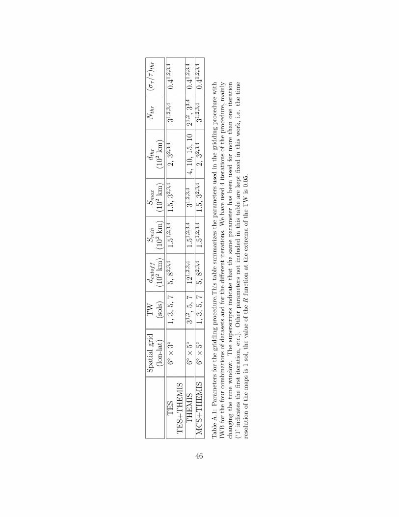
Spat

ial

grid

TW

dcutoff

Smin

Smax

dthr

Nthr

(στ/τ

) thr

(lon

-lat

)(s

ols)

(102

km

)(1

02km

)(1

02km

)(1

02km

)

TE

S6◦×

3◦1,

3,5,

75,

82,3,4

1.51,2,3,4

1.5,

32,3,4

2,32,3,4

31,2,3,4

0.41,2,3,4

TE

S+

TH

EM

IST

HE

MIS

6◦×

5◦31,2

,5,

712

1,2,3,4

1.51,2,3,4

31,2,3,4

4,10

,15

,10

21,2

,33,4

0.41,2,3,4

MC

S+

TH

EM

IS6◦×

5◦1,

3,5,

75,

82,3,4

1.51,2,3,4

1.5,

32,3,4

2,32,3,4

31,2,3,4

0.41,2,3,4

Tab

leA

.1:

Par

amet

ers

for

the

grid

din

gp

roce

du

re.T

his

tab

lesu

mm

ari

zes

the

para

met

ers

use

din

the

gri

dd

ing

pro

ced

ure

wit

hIW

Bfo

rth

efo

ur

com

bin

atio

ns

ofd

atas

ets

and

for

the

diff

eren

tit

erati

on

s.W

eh

ave

use

d4

iter

ati

on

sof

the

pro

ced

ure

,m

ain

lych

angi

ng

the

tim

ew

ind

ow.

Th

esu

per

scri

pts

ind

icate

that

the

sam

ep

ara

met

erh

as

bee

nu

sed

for

more

than

on

eit

erati

on

(‘1’

ind

icat

esth

efi

rst

iter

atio

n,

etc.

).O

ther

para

met

ers

not

incl

ud

edin

this

tab

leare

kep

tfi

xed

inth

isw

ork

,i.

e.th

eti

me

reso

luti

onof

the

map

sis

1so

l,th

eva

lue

ofth

eR

fun

ctio

nat

the

extr

ema

of

the

TW

is0.0

5.

46

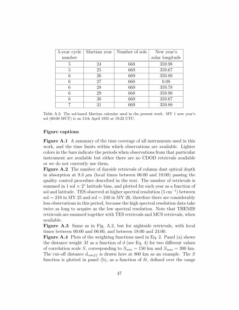
5-year cycle Martian year Number of sols New year’snumber solar longitude

5 24 668 359.985 25 669 359.676 26 669 359.886 27 668 0.086 28 669 359.786 29 668 359.986 30 669 359.677 31 669 359.88

Table A.2: The sol-based Martian calendar used in the present work. MY 1 new year’ssol (00:00 MUT) is on 11th April 1955 at 19:22 UTC.

Figure captions

Figure A.1 A summary of the time coverage of all instruments used in thiswork, and the time limits within which observations are available. Lightercolors in the bars indicate the periods when observations from that particularinstrument are available but either there are no CDOD retrievals availableor we do not currently use them.Figure A.2 The number of dayside retrievals of column dust optical depthin absorption at 9.3 µm (local times between 06:00 and 18:00) passing thequality control procedure described in the text. The number of retrievals issummed in 1 sol × 2◦ latitude bins, and plotted for each year as a function ofsol and latitude. TES observed at higher spectral resolution (5 cm−1) betweensol ∼ 210 in MY 25 and sol ∼ 240 in MY 26, therefore there are considerablyless observations in this period, because the high spectral resolution data taketwice as long to acquire as the low spectral resolution. Note that THEMISretrievals are summed together with TES retrievals and MCS retrievals, whenavailable.Figure A.3 Same as in Fig. A.2, but for nightside retrievals, with localtimes between 00:00 and 06:00, and between 18:00 and 24:00.Figure A.4 Plots of the weighting functions used in Eq. 2. Panel (a) showsthe distance weight M as a function of d (see Eq. 4) for two different valuesof correlation scale S, corresponding to Smin = 150 km and Smax = 300 km.The cut-off distance dcutoff is drawn here at 800 km as an example. The Sfunction is plotted in panel (b), as a function of δt, defined over the range

47

−3.5 < δt < 3.5 for TW=7 sol. In panel (c) we plot the time weight functionR (see Eq. 6) for the same TW=7 sol. The value of the R function at theextrema of the time window interval is fixed to 0.05 in this work. Finally,panel (d) shows the plot of the uncertainty weight Q (see Eq. 7) as a functionof the relative uncertainty σtau/τ , where σ is the standard deviation of a singlecolumn dust optical depth retrieval τ .Figure A.5 The difference between the time of each TES observation andnoon at 0◦ longitude in sol 449, Ls = 227.8◦, MY 24 (the ‘current time’). Theobservations are shown within a time window of 7 sols centered around thecurrent time. The picture is a zoomed view centered around 10◦ longitudeand −25◦ latitude. The black square shows a 6◦ × 3◦ longitude-latitude boxwhereas the black circle indicates the 800 km distance range (dcutoff ) we usein the weighted binning for the TES dataset when the time window is 7 sols(see Table A.1). We apply the time and spatial weighting within this circle,as detailed in Section 3.2.Figure A.6 (a) The panels from top to bottom show TES observationsaccumulated within time windows of 1, 3, 5 and 7 sol, centred around noonat 0◦ longitude in sol 449. (b) The panels from top to bottom show the cor-responding partial results of the application of the weighted binning for eachspecific time window. Finally, in panel (c) we show the result of the iterativeapplication of all 4 TW, where the valid grid points in each iteration are notoverwritten. There are 60x60 grid points in the gridded maps, separated by6◦ × 3◦ in longitude and latitude. Missing values are assigned to bins wherethe acceptance criterion is not satisfied (see Table A.1).Figure A.7 Tests on the sensitivity of the gridding procedure on the spatialresolution. We use the same sol as in Fig. A.6. Panel (a) and (f) show thecase with 5◦ × 5◦ longitude-latitude resolution, respectively in the averageand in the standard deviation fields; panel (b) and (g) are for the case with6◦×3◦ resolution; panel (c) and (h) are for the case with 6◦×3◦ resolution butlonger range for the space weighting (Smin = 250 km and Smax = 400 km);panel (d) and (i) are for the case with 8◦ × 2◦ resolution.Figure A.8 Evolution of the MY 24, Ls ∼ 227◦ flushing storm. Each panelshows gridded column dust optical depth (in absorption at 9.3 µm) at thereference pressure level of 610 Pa. From top left to bottom right, maps areprovided from sol 440 to sol 451 (i.e. from Ls ∼ 221.4◦ to Ls ∼ 228.4◦). In allpanels, MUT is noon and solar longitudes are provided accordingly. See alsoAppendix A for the description of the sol-based Martian calendar we use inthis paper.

48

Figure A.9 Evolution of the MY 29, Ls ∼ 235◦ regional storm. As inFig. A.8, each panel shows gridded column dust optical depth (in absorptionat 9.3 µm) at reference pressure level of 610 Pa. From top left to bottomright, maps are provided from sol 457 to sol 468 (i.e. from Ls ∼ 232.3◦ toLs ∼ 239.4◦).Figure A.10 Histograms of SMD values (Eq. 8) for TES and MCS datasetsin different Martian years: (a) TES, MY 24; (b) TES, MY 25; (c) TES,MY 26; (d) MCS, MY 28; (e) MCS, MY 29; (f) MCS, MY 30; (g) MCS,MY 31.Figure A.11 Plots of relative standard deviation curves for different Mar-tian years. The relative standard deviation is defined as the ratio betweenthe weighted standard deviation and the weighted average calculated, respec-tively, with Eq. 2 and Eq. 3, for each valid grid point.Figure A.12 Histograms of SMD values (Eq. 8) for the CRISM dataset indifferent Martian years: (a) MY 28; (b) MY 29; (c) MY 30.Figure A.13 Plot of column dust optical depth time series at (a) Spiritsite in Gusev crater, and (b) Opportunity site in Meridiani Planum. Thered curves are the time series of values interpolated from the daily griddedmaps obtained with IWB procedure (only values where 4 neighbor grid pointsare valid). The green curves are sol-averaged values from MER Mini-TES,whereas the blue curves are sol-averaged values from MER PanCam. Corre-sponding uncertainty values are drawn as gray envelopes. Values interpolatedfrom the gridded maps and Mini-TES values are multiplied by 2.6 to convertthem from absorption at 9.3 µm to equivalent visible, to compare to PanCamvalues at 800 nm.Figure A.14 Tracks of TES column dust optical depth (at 9.3 µm in ab-sorption) overlaid on MOC Mars Daily Global Map images for 6 sols at 2 solintervals in MY 24. Contours show the analyzed optical depth from the grid-ded maps derived from TES observations as described in the text. (a) Sol 440(Ls = 221.4◦), (b) Sol 442 (Ls = 222.6◦), (c) Sol 444 (Ls = 223.9◦), (d) Sol446 (Ls = 225.2◦), (e) Sol 448 (Ls = 226.5◦), and (f) Sol 450 (Ls = 227.8◦). Inall maps, MUT is noon, and solar longitude values are provided accordingly.See Appendix A for the description of the sol-based Martian calendar we usein this paper. MOC images are provided by Bruce Cantor.Figure A.15 Tracks of surface temperature anomaly overlaid on MARCIMars Daily Global Map images for (a) Sol 460 (Ls = 234.2◦) and (b) Sol468 (Ls = 239.4◦). See Appendix A for the description of the sol-basedMartian calendar we use in this paper. Brightness temperature anomaly is

49

the apparent decrease in afternoon surface temperature (32 micron brightnesstemperature), relative to a clear atmosphere, that can be attributed to theinfluence of dust. MARCI images are provided by Helen Wang.Figure A.16 Zonal means of 9.3 µm absorption column dust optical depthmaps (referred to 610 Pa) as a function of solar longitude and latitude forall eight available Martian years. Data are extracted from the irregularlygridded maps obtained with the application of the IWR procedure.Figure A.17 Plot of the zonal mean of the 9.3 µm absorption column dustoptical depth in the climatological year, as a function of solar longitude andlatitude. The climatological year is obtained by averaging the irregularlygridded maps for all eight years, excluding the largest value of CDOD foreach grid point.Figure A.18 Plot of equatorial (5◦ S–5◦ N) 9.3 µm absorption column dustoptical depth as a function of solar longitude for all eight Martian years.Figure A.19 Plots of 9.3 µm absorption column dust optical depth as afunction of latitude for all eight Martian years, at two seasons: (a) Ls =[95◦, 105◦], and (b) Ls = [295◦, 305◦].Figure A.20 Map of 9.3 µm absorption column dust optical depth corre-sponding to Fig. A.6 (sol 449, MY 24) after the application of kriging at highresolution. The map is regular and complete, on a 2◦× 2◦ longitude-latitudegrid.Figure A.21 Zonal means of 9.3 µm absorption column dust optical depthmaps (referred to 610 Pa) as a function of solar longitude and latitude for alleight available Martian years, calculated using the complete maps after theapplication of the kriging procedure.

50

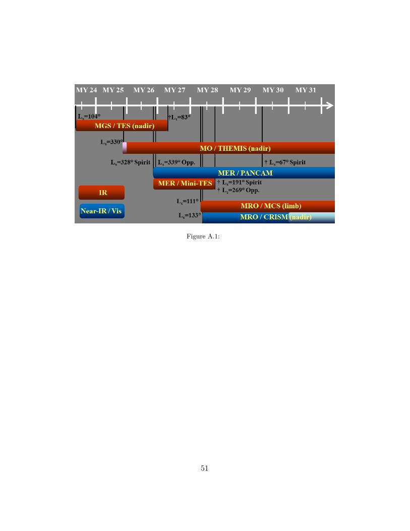
Figure A.1:

51

Figure A.2:

52

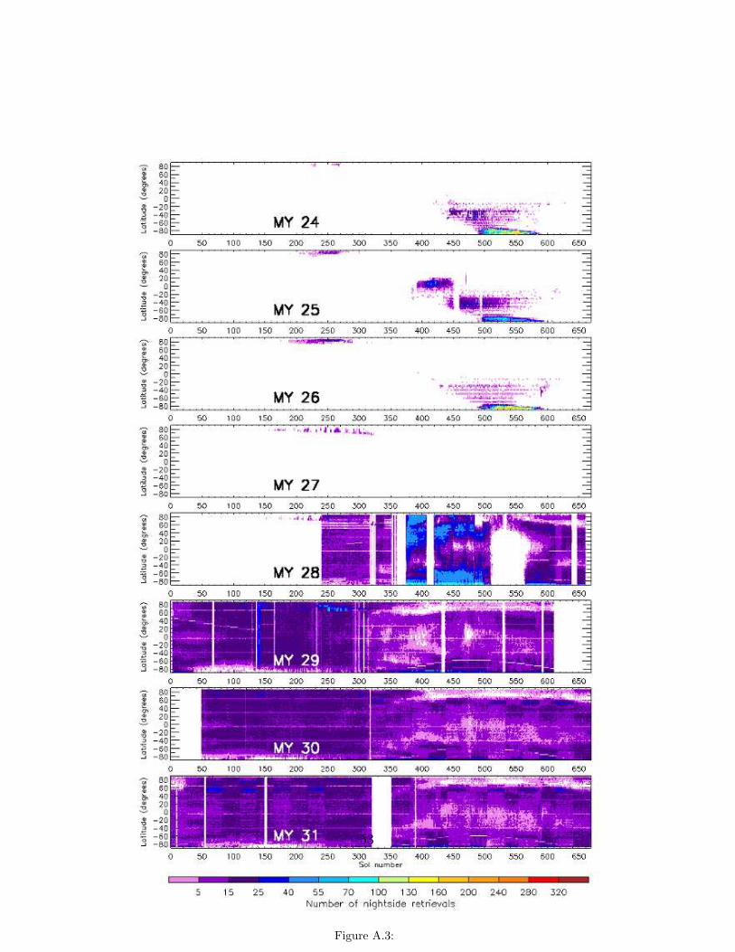
Figure A.3:

53

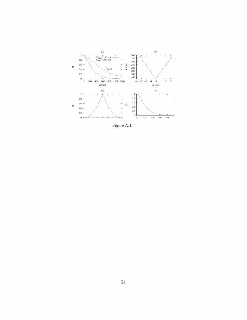
0

0.2

0.4

0.6

0.8

1

0 200 400 600 800 1000 1200

M

d (km)

(a)

dcutoff

Smin = 150 kmSmax = 300 km

160 180 200 220 240 260 280 300

-4 -3 -2 -1 0 1 2 3 4

S (k

m)

δt (sol)

(b)

0

0.2

0.4

0.6

0.8

1

R

(c)

0

0.2

0.4

0.6

0.8

1

0 0.2 0.4 0.6 0.8 1

Q

(c)

Figure A.4:

54

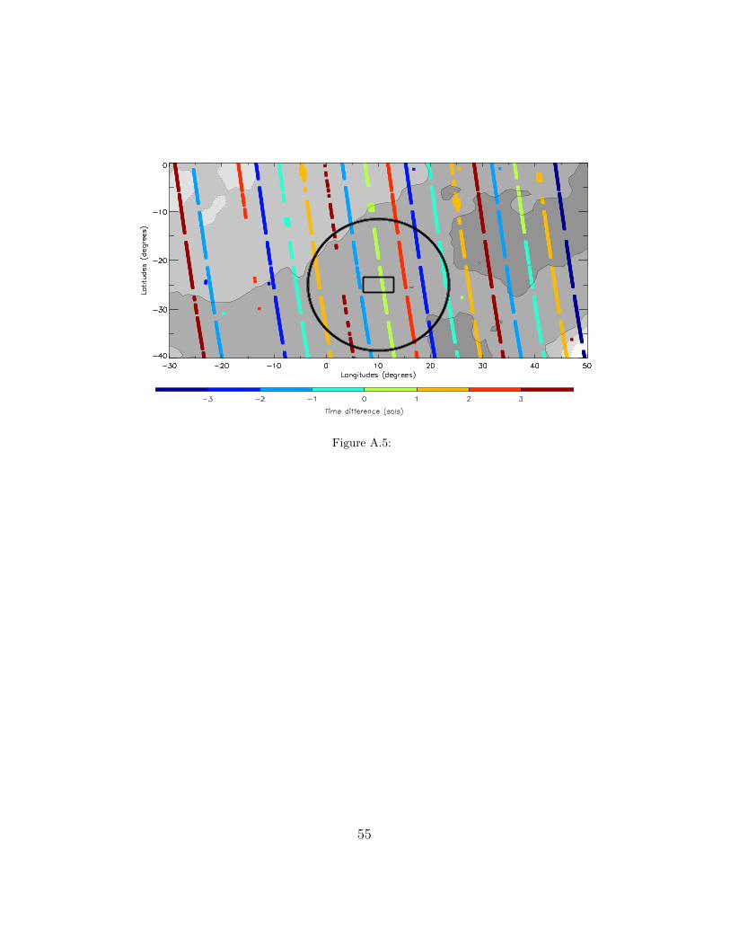
Figure A.5:

55

Figure A.6:

56

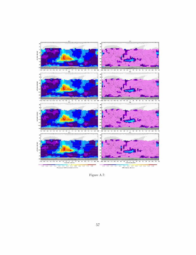
Figure A.7:

57

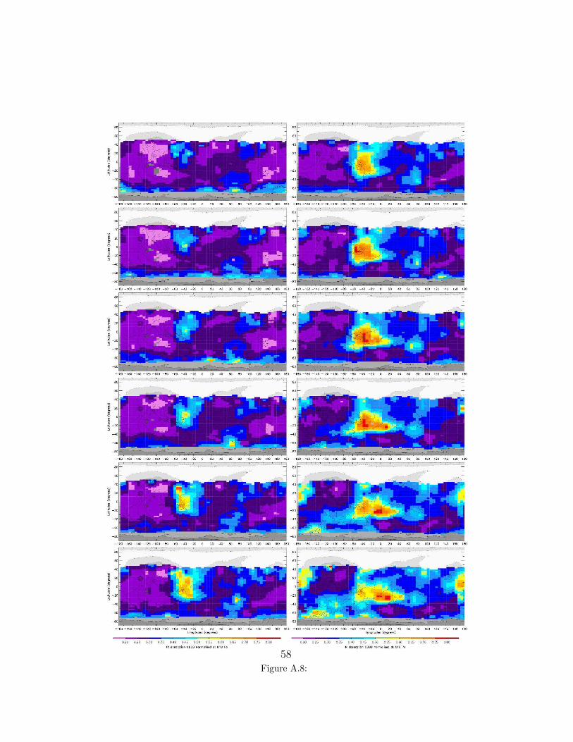
Figure A.8:

58

Figure A.9:

59

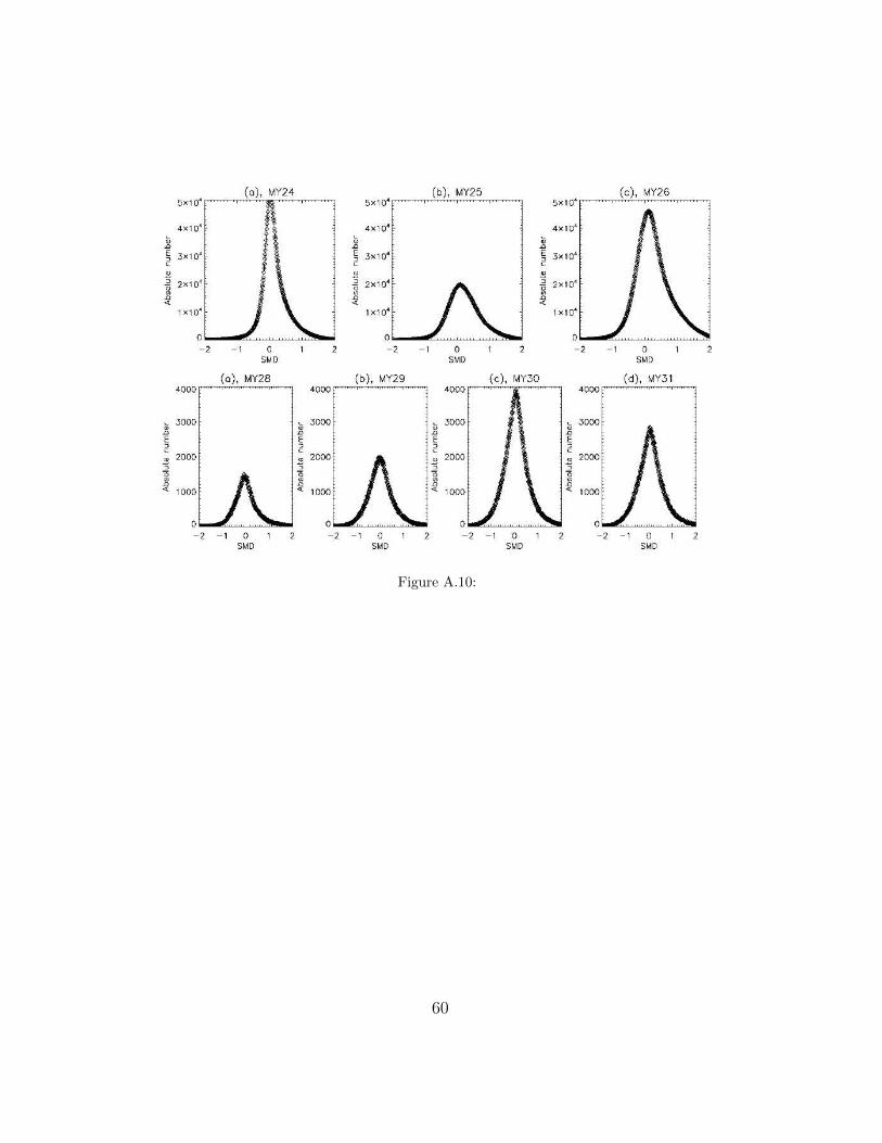
Figure A.10:

60

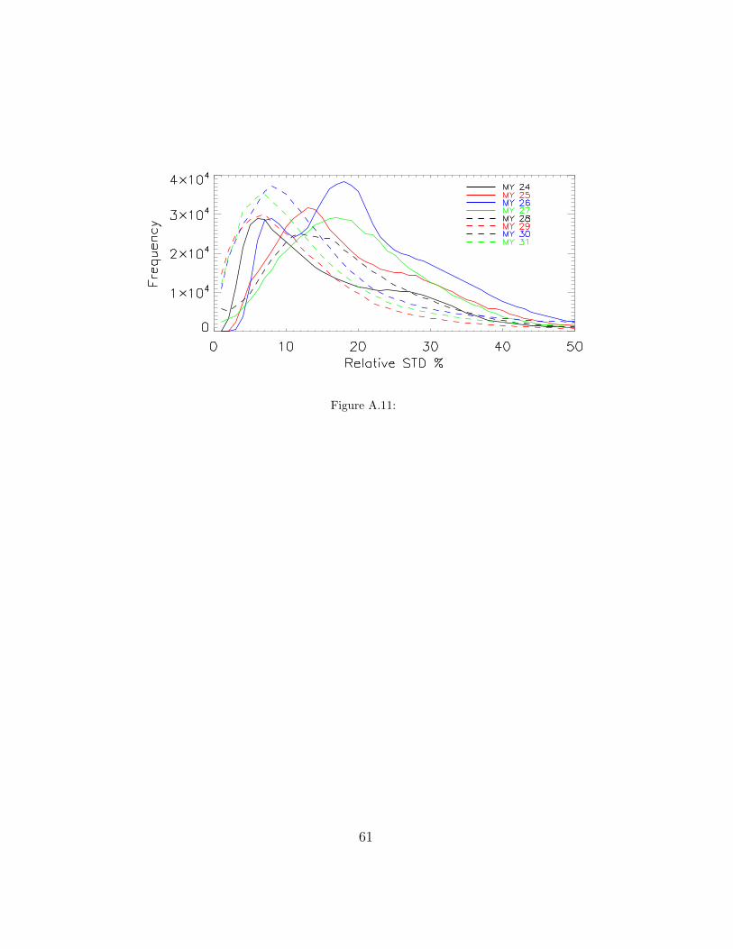
Figure A.11:

61

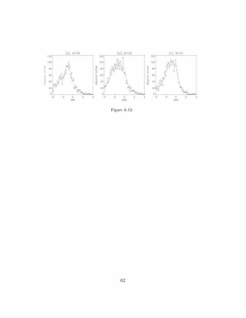
Figure A.12:

62

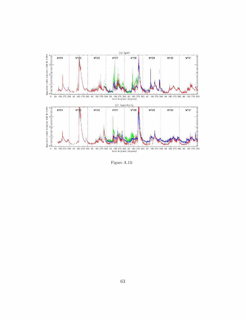
Figure A.13:

63

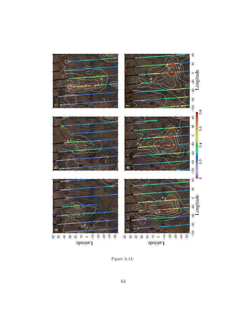
Figure A.14:

64

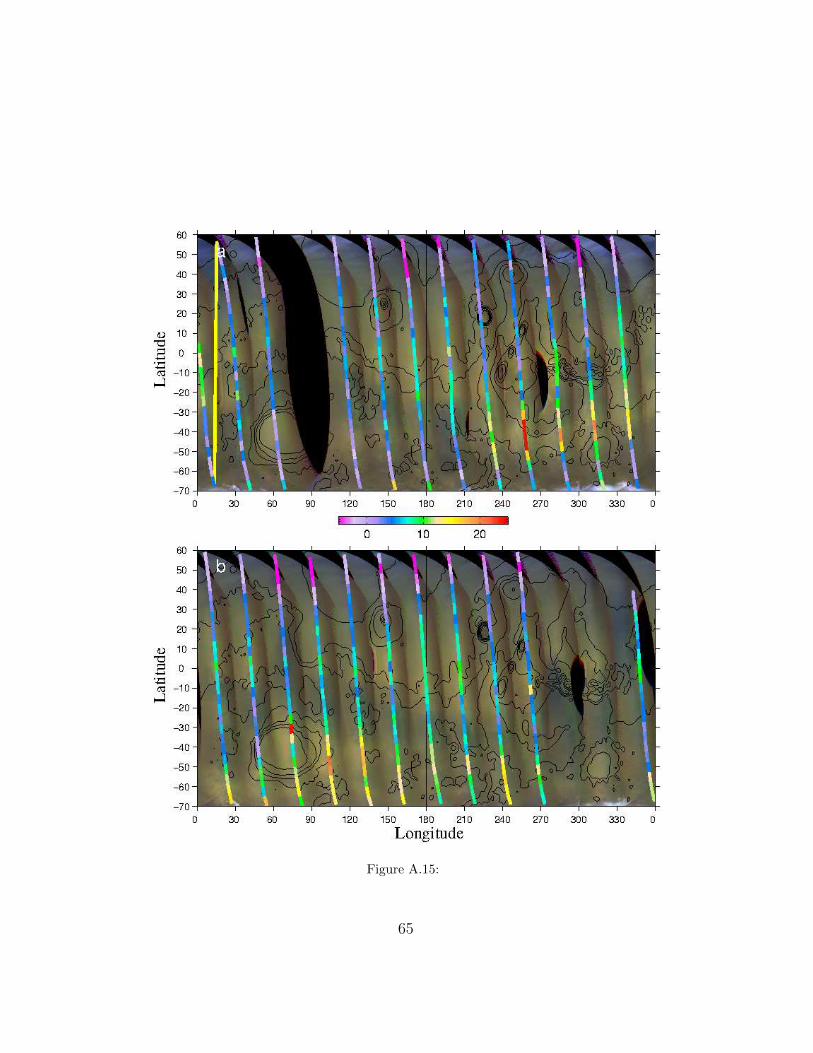
Figure A.15:

65

Figure A.16:

66

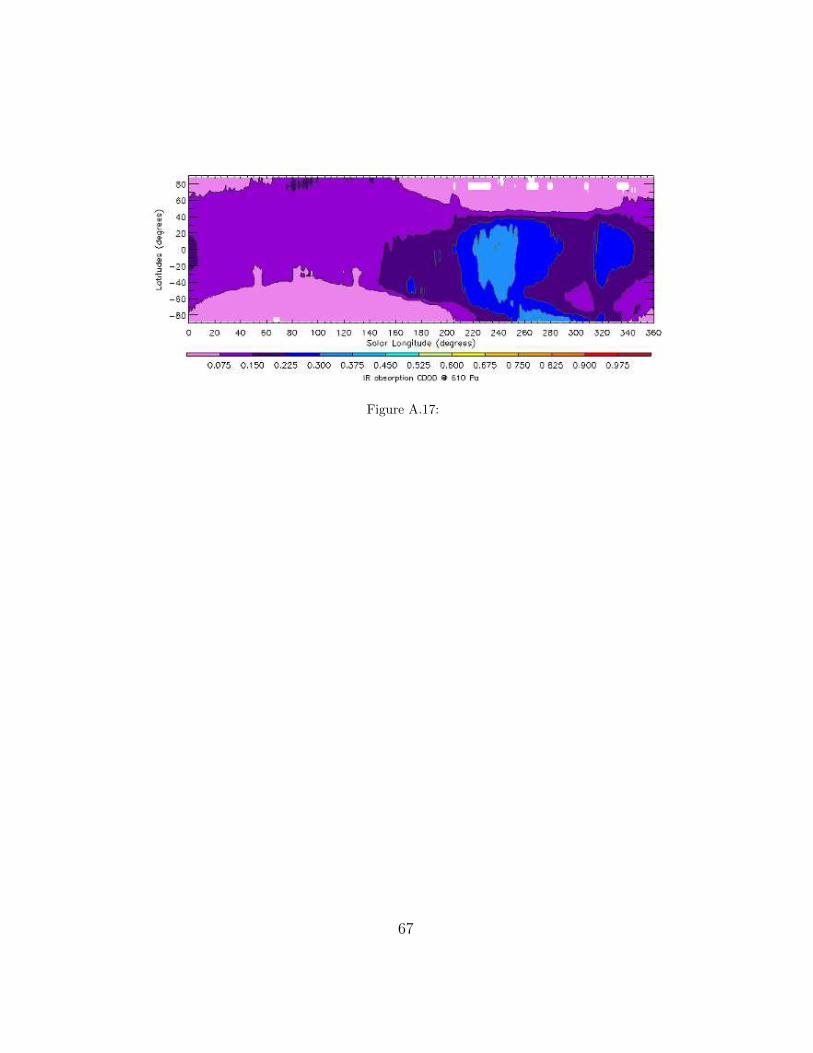
Figure A.17:

67

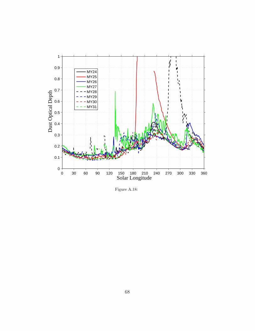
Solar Longitude

Dus

t Opt

ical

Dep

th

0 30 60 90 120 150 180 210 240 270 300 330 3600

0.1

0.2

0.3

0.4

0.5

0.6

0.7

0.8

0.9

1

MY24MY25MY26MY27MY28MY29MY30MY31

Figure A.18:

68

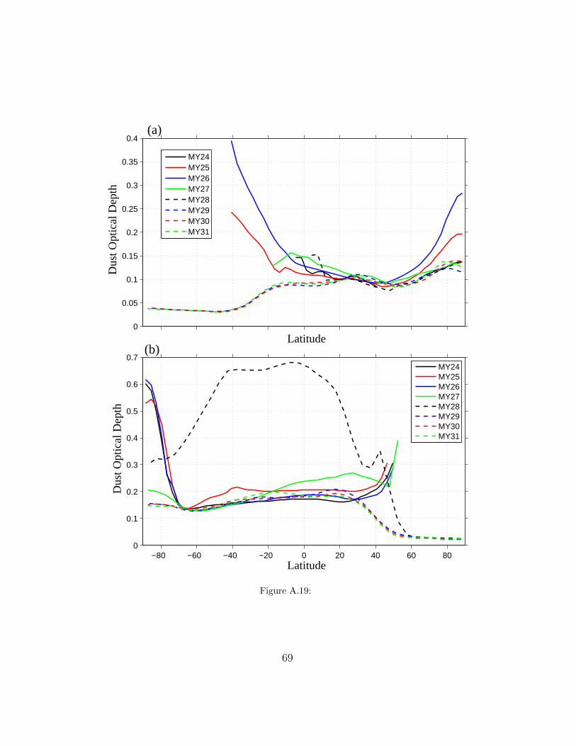
Latitude

Dus

t Opt

ical

Dep

th

(a)

0

0.05

0.1

0.15

0.2

0.25

0.3

0.35

0.4

Latitude

Dus

t Opt

ical

Dep

th

(b)

−80 −60 −40 −20 0 20 40 60 800

0.1

0.2

0.3

0.4

0.5

0.6

0.7

MY24MY25MY26MY27MY28MY29MY30MY31

MY24MY25MY26MY27MY28MY29MY30MY31

Figure A.19:

69

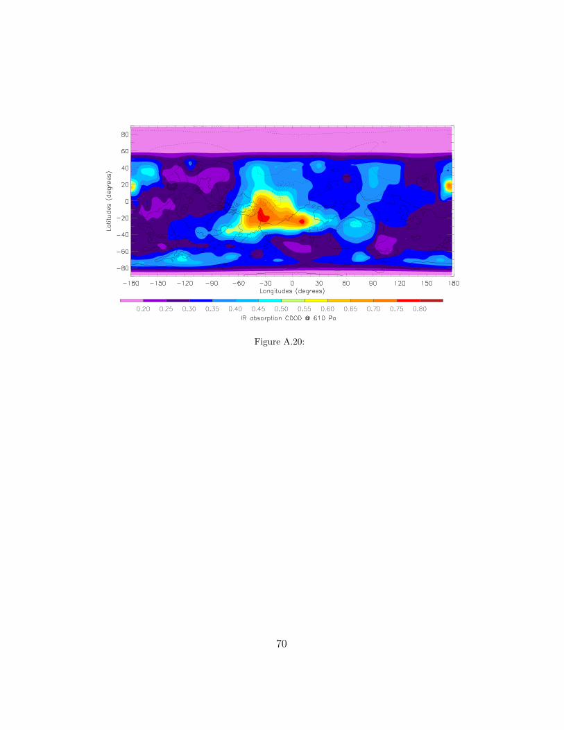
Figure A.20:

70

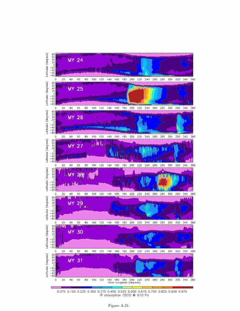
Figure A.21:

71