efficient evidence accumulation clustering for large ... · efficient evidence accumulation...
TRANSCRIPT

Efficient Evidence Accumulation Clustering for largedatasets/big data
Diogo Alexandre Oliveira Silva
Thesis to obtain the Master of Science Degree in
Electrical and Computer Engineering
Supervisors: Dra. Ana Luísa Nobre FredDra. Helena Isabel Aidos Lopes
Examination Committee
Chairperson: Prof. Dr. João Fernando Cardoso Silva SequeiraSupervisor: Dra. Ana Luísa Nobre Fred
Members of the Committee: Dr. Pedro Filipe Zeferino TomásBGEN ENGEL José Manuel dos Santos Vicêncio
TCOR ENGEL Ana Paula da Silva Jorge
December 2015

ii

Acknowledgments
It would come as a great oversight if I was not aware of the help and contribution I received for the
completion of this undertaking.
I should start by expressing deep appreciation to my supervisors, Dr. Ana Fred and Dr. Helena
Lopes. The freedom I was allowed was crucial for keeping my motivation up for such a long period.
When that was lacking, their guidance and encouragement quickly put me back on track.
I leave my warmest regards to the family I built throughout my military and academic career, during
these last years. Your camaraderie has shaped where I stand and who I am today. Your support
throughout these long months was invaluable.
To my loving girlfriend, who would always hear my boundless enthusiasm or disheartening frustra-
tions, whichever was the case, and who followed me closest in the last months, I am deeply grateful.
You motivated me most of all, and that was no small task.
And to my parents, thank you for all your support and motivation during all these years. You were
always caring and encouraging and I am forever grateful for that.
Last, but not least, thank you to all my friends and family for understanding my absence during these
challenging months.
iii

iv

Resumo
Avancos na tecnologia permitem a recolha e armazenamento de quantidades e variedades de dados
sem precedente. A maior parte destes dados sao armazenados eletronicamente e existe interesse em
realizar analise automatica dos mesmos. As tecnicas de clustering estao entre as mais populares para
essa tarefa porque nao assumem nada sobre a estrutura dos dados a priori. Muitas tecnicas existem,
mas, tıpicamente, nao tem um bom desempenho em todos os conjuntos de dados devido as especi-
fidades de cada um. Tecnicas de ensemble clustering tentam responder a esse desafio ao combinar
outros algoritmos. Esta dissertacao foca-se numa em particular, o Evidence Accumulation Clustering
(EAC). O EAC e uma algorithm robusto que tem demonstrado bons desempenhos na literatura numa
variedade de conjuntos de dados. No entanto, esta robustez vem com um maior custo computacional
associado. A sua aplicacao nao so e mais lenta como esta restrita a conjuntos de dados pequenos.
Assim, o objetivo desta dissertacao e escalar o EAC, possibilitando a sua a aplicacao a conjuntos de
dados grandes, com tecnologia disponivel numa tıpica estacao de trabalho. Com isto em mente, varias
abordagens foram exploradas: acelerar processamento com outros algoritmos (quantum clustering),
atraves de processamento paralelo (com GPU), escalar com algoritmos de memoria externa (disco
rıgido) e explorando a natureza esparsa do EAC. Alem disto, foi desenvolvido um metodo eficiente para
construir uma matriz esparsa especıfico ao EAC. A solucao proposta e aplicavel a conjuntos de dados
grandes e e entre 6 a 200 vezes mais rapida que a original para conjuntos pequenos.
Palavras-chave: Metodos de agrupamento, EAC, K-Means, MST, GPGPU, CUDA, Matrizes
esparsas, Single-Link
v

vi

Abstract
Advances in technology allow for the collection and storage of an unprecedent amount and variety of
data. Most of this data is stored electronically and there is an interest in automated analysis for gener-
ation of knowledge and new insights. Since the structure of the data is unknown, clustering techniques
become particularly interesting for knowledge discovery and data mining, as they make as few assump-
tions on the data as possible. A vast body of work on these algorithms exist, yet, typically, no single
algorithm is able to respond to the specificities of all data. Ensemble clustering algorithm address this
problem by combining other algorithms. Evidence Accumulation Clustering (EAC) is a robust ensemble
algorithm that has shown good results and is the focus of this dissertation. However, this robustness
comes with higher computational cost. Its application is slower and restricted to smaller datasets. Thus,
the objective of this dissertation is to scale EAC, allowing its applicability to big datasets, with technology
available at a typical workstation. Accordingly, several approaches were explored: speed-up with other
algorithms (quantum clustering) or parallel computing (with GPU) and reducing space complexity by
using external memory (hard drive) algorithms and exploiting the sparse nature of EAC. A relevant con-
tribution is a novel method to build a sparse matrix specialized in EAC. Results show that the proposed
solution is applicable to large datasets and presents speed-ups between 6 and 200 over the original
implementation on different phases of EAC for small datasets.
Key words: Clustering methods, EAC, K-Means, MST, GPGPU, CUDA, Sparse matrices,
Single-Link
vii

viii

Contents
Acknowledgments . . . . . . . . . . . . . . . . . . . . . . . . . . . . . . . . . . . . . . . . . . . iii
Resumo . . . . . . . . . . . . . . . . . . . . . . . . . . . . . . . . . . . . . . . . . . . . . . . . . v
Abstract . . . . . . . . . . . . . . . . . . . . . . . . . . . . . . . . . . . . . . . . . . . . . . . . . vii
List of Tables . . . . . . . . . . . . . . . . . . . . . . . . . . . . . . . . . . . . . . . . . . . . . . xiv
List of Figures . . . . . . . . . . . . . . . . . . . . . . . . . . . . . . . . . . . . . . . . . . . . . xvi
Glossary . . . . . . . . . . . . . . . . . . . . . . . . . . . . . . . . . . . . . . . . . . . . . . . . xvii
1 Introduction 1
1.1 Challenges and Motivation . . . . . . . . . . . . . . . . . . . . . . . . . . . . . . . . . . . . 1
1.2 Goals . . . . . . . . . . . . . . . . . . . . . . . . . . . . . . . . . . . . . . . . . . . . . . . 2
1.3 Contributions . . . . . . . . . . . . . . . . . . . . . . . . . . . . . . . . . . . . . . . . . . . 2
1.4 Outline . . . . . . . . . . . . . . . . . . . . . . . . . . . . . . . . . . . . . . . . . . . . . . . 3
2 Clustering: basic concepts, definitions and algorithms 4
2.1 The problem of clustering . . . . . . . . . . . . . . . . . . . . . . . . . . . . . . . . . . . . 4
2.2 Definitions and Notation . . . . . . . . . . . . . . . . . . . . . . . . . . . . . . . . . . . . . 5
2.3 Characteristics of clustering techniques . . . . . . . . . . . . . . . . . . . . . . . . . . . . 7
2.4 K-Means . . . . . . . . . . . . . . . . . . . . . . . . . . . . . . . . . . . . . . . . . . . . . 8
2.5 Single-Link . . . . . . . . . . . . . . . . . . . . . . . . . . . . . . . . . . . . . . . . . . . . 10
2.6 Ensemble Clustering . . . . . . . . . . . . . . . . . . . . . . . . . . . . . . . . . . . . . . . 12
2.7 Evidence Accumulation Clustering . . . . . . . . . . . . . . . . . . . . . . . . . . . . . . . 12
2.7.1 Overview . . . . . . . . . . . . . . . . . . . . . . . . . . . . . . . . . . . . . . . . . 12
3 State of the art 15
3.1 Scalability of EAC . . . . . . . . . . . . . . . . . . . . . . . . . . . . . . . . . . . . . . . . 15
3.1.1 p neighbors approach . . . . . . . . . . . . . . . . . . . . . . . . . . . . . . . . . . 16
3.1.2 Increased sparsity approach . . . . . . . . . . . . . . . . . . . . . . . . . . . . . . 16
3.2 Clustering with large datasets . . . . . . . . . . . . . . . . . . . . . . . . . . . . . . . . . . 17
3.2.1 Parallel K-Means . . . . . . . . . . . . . . . . . . . . . . . . . . . . . . . . . . . . . 18
3.2.2 Parallel Single-Link Clustering . . . . . . . . . . . . . . . . . . . . . . . . . . . . . 18
3.3 Quantum clustering . . . . . . . . . . . . . . . . . . . . . . . . . . . . . . . . . . . . . . . 26
3.3.1 The quantum bit approach . . . . . . . . . . . . . . . . . . . . . . . . . . . . . . . 27
ix

3.3.2 Schrodinger’s equation approach . . . . . . . . . . . . . . . . . . . . . . . . . . . . 30
4 EAC for large datasets: proposed solutions 32
4.1 Quantum Clustering . . . . . . . . . . . . . . . . . . . . . . . . . . . . . . . . . . . . . . . 33
4.2 Speeding up Ensemble Generation with Parallel K-Means . . . . . . . . . . . . . . . . . . 34
4.2.1 Maximum potential speed-up . . . . . . . . . . . . . . . . . . . . . . . . . . . . . . 34
4.2.2 Implementation details . . . . . . . . . . . . . . . . . . . . . . . . . . . . . . . . . . 34
4.3 Dealing with the space complexity of the co-association matrix . . . . . . . . . . . . . . . 36
4.4 Building the sparse matrix . . . . . . . . . . . . . . . . . . . . . . . . . . . . . . . . . . . . 37
4.4.1 EAC CSR . . . . . . . . . . . . . . . . . . . . . . . . . . . . . . . . . . . . . . . . . 37
4.4.2 EAC CSR Condensed . . . . . . . . . . . . . . . . . . . . . . . . . . . . . . . . . . 40
4.5 Final partition recovery . . . . . . . . . . . . . . . . . . . . . . . . . . . . . . . . . . . . . . 42
4.5.1 Single-Link and GPGPU . . . . . . . . . . . . . . . . . . . . . . . . . . . . . . . . . 43
4.5.2 Single-Link and external memory algorithms . . . . . . . . . . . . . . . . . . . . . 47
4.6 Overview of the developed work . . . . . . . . . . . . . . . . . . . . . . . . . . . . . . . . 49
4.7 Guidelines for using the different solutions . . . . . . . . . . . . . . . . . . . . . . . . . . . 49
5 Results and Discussion 51
5.1 Experimental environment . . . . . . . . . . . . . . . . . . . . . . . . . . . . . . . . . . . . 51
5.2 Quantum Clustering . . . . . . . . . . . . . . . . . . . . . . . . . . . . . . . . . . . . . . . 53
5.2.1 Quantum K-Means . . . . . . . . . . . . . . . . . . . . . . . . . . . . . . . . . . . . 53
5.2.2 Horn and Gottlieb’s algorithm . . . . . . . . . . . . . . . . . . . . . . . . . . . . . . 54
5.3 Parallel K-Means . . . . . . . . . . . . . . . . . . . . . . . . . . . . . . . . . . . . . . . . . 55
5.3.1 Analysis of speed-up . . . . . . . . . . . . . . . . . . . . . . . . . . . . . . . . . . . 56
5.3.2 Effective bandwidth and computational throughput . . . . . . . . . . . . . . . . . . 57
5.3.3 Influence of the number of points per thread . . . . . . . . . . . . . . . . . . . . . . 58
5.4 Building the co-association matrix with different sparse formats . . . . . . . . . . . . . . . 58
5.5 GPU MST . . . . . . . . . . . . . . . . . . . . . . . . . . . . . . . . . . . . . . . . . . . . . 59
5.6 EAC Validation . . . . . . . . . . . . . . . . . . . . . . . . . . . . . . . . . . . . . . . . . . 62
5.7 EAC . . . . . . . . . . . . . . . . . . . . . . . . . . . . . . . . . . . . . . . . . . . . . . . . 63
5.7.1 Performance of production and combination phases . . . . . . . . . . . . . . . . . 64
5.7.2 Performance comparison between SLINK, SL-MST and SL-MST-Disk . . . . . . . 66
5.7.3 Performance of all phases combined . . . . . . . . . . . . . . . . . . . . . . . . . . 66
5.7.4 Analysis of the number of associations . . . . . . . . . . . . . . . . . . . . . . . . . 67
5.7.5 Space complexity . . . . . . . . . . . . . . . . . . . . . . . . . . . . . . . . . . . . 70
5.7.6 Accuracy . . . . . . . . . . . . . . . . . . . . . . . . . . . . . . . . . . . . . . . . . 71
5.8 Performance on real world datasets . . . . . . . . . . . . . . . . . . . . . . . . . . . . . . 72
x

6 Conclusions 74
6.1 Achievements . . . . . . . . . . . . . . . . . . . . . . . . . . . . . . . . . . . . . . . . . . . 74
6.2 Future Work . . . . . . . . . . . . . . . . . . . . . . . . . . . . . . . . . . . . . . . . . . . . 75
References 87
A General Purpose computing on Graphical Processing Units 89
A.1 Programming GPUs . . . . . . . . . . . . . . . . . . . . . . . . . . . . . . . . . . . . . . . 89
A.2 OpenCL vs CUDA . . . . . . . . . . . . . . . . . . . . . . . . . . . . . . . . . . . . . . . . 90
A.3 Overview of CUDA . . . . . . . . . . . . . . . . . . . . . . . . . . . . . . . . . . . . . . . . 90
xi

xii

List of Tables
4.1 Maximum theoretical speed-up for the labeling and update phases of K-Means based on
experimental data. The datasets used range from 1000 to 500 000 patterns, from 2 to 1000
dimensions and from 2 to 2048 centroids. . . . . . . . . . . . . . . . . . . . . . . . . . . . 35
4.2 Memory used for different matrix types for the generic case and a real example of 100000
patterns. The relative reduction (R.R.) refers to the memory reduction relative to the type
of matrix above, the absolute reduction (A.R.) refers to the reduction relative to the full
complete matrix. . . . . . . . . . . . . . . . . . . . . . . . . . . . . . . . . . . . . . . . . . 42
5.1 Alpha machine specifications. . . . . . . . . . . . . . . . . . . . . . . . . . . . . . . . . . 52
5.2 Bravo machine specifications. . . . . . . . . . . . . . . . . . . . . . . . . . . . . . . . . . 52
5.3 Charlie machine specifications. . . . . . . . . . . . . . . . . . . . . . . . . . . . . . . . . . 53
5.4 Timing results for the different algorithms in the different tests. Fitness time refers to the
time that took to compute the DB index of each solution of classical K-Means. All time
values are the average over 20 rounds and are displayed in seconds. . . . . . . . . . . . 54
5.5 All values displayed are the average over 20 rounds, except for the Overall best which
shows the best result in any round. The values represent the Davies-Bouldin fitness
index (low is better). . . . . . . . . . . . . . . . . . . . . . . . . . . . . . . . . . . . . . . . 55
5.6 Time of computation of Horn and Gottlieb [76] algorithm for a mixture of 4 Gaussians of
different cardinality and dimensionality. . . . . . . . . . . . . . . . . . . . . . . . . . . . . . 55
5.7 Effective bandwidth and computational throughput of labeling phase computed from re-
sults taken from running K-Means over datasets whose complexity ranged from 100 to
10 000 000 patterns, from 2 to 1000 dimensions and from 2 to 2048 centroids. . . . . . . . . 58
5.8 Speed-up obtained in the labeling phase for different number of patterns per thread (PPT). 58
5.9 Execution times for computing the condensed co-association matrix using different matrix
strategies. . . . . . . . . . . . . . . . . . . . . . . . . . . . . . . . . . . . . . . . . . . . . . 59
5.10 Average speed-up of the GPU MST algorithm for different data sets, sorted by number of
edges. . . . . . . . . . . . . . . . . . . . . . . . . . . . . . . . . . . . . . . . . . . . . . . . 60
5.11 Cross-correlation between several characteristics of the graphs and the average speed-up. 61
5.12 Difference between accuracies from the two implementations of EAC, using the same
ensemble. Accuracy was measured using the H-index. . . . . . . . . . . . . . . . . . . . . 62
xiii

5.13 Speed-ups obtained in the different phases of EAC, with independent production of en-
sembles. . . . . . . . . . . . . . . . . . . . . . . . . . . . . . . . . . . . . . . . . . . . . . . 63
5.14 Different rules for computing Kmin and Kmax. n is the number of patterns and sk is the
number of patterns per cluster. . . . . . . . . . . . . . . . . . . . . . . . . . . . . . . . . . 63
5.15 Execution times for real-world large datasets. P and F refer to the number of patterns and
features. P, C and R times refer to the production, combination and recovery times. . . . . 73
xiv

List of Figures
2.1 First and second features of the Iris dataset. Fig. 2.1a shows the scatter plot of the raw
input data, i.e. how the algorithms ”see” the data. Fig. 2.1b shows the desired labels for
each point, where each color and symbol are coded to a class. . . . . . . . . . . . . . . . 5
2.2 The output labels of the K-Means algorithm with the number of clusters (input parameter)
set to 3. The different plots show the centroids (squares) evolution on each iteration.
Between iteration 3 and the converged state 2 more iterations were executed. . . . . . . . 9
2.3 The above figures show an example of a graph (left) and its corresponding Minimum
Spanning Tree (right). The circles are vertices and the edges are the lines linking the
vertices. . . . . . . . . . . . . . . . . . . . . . . . . . . . . . . . . . . . . . . . . . . . . . . 11
2.4 The above plots show the dendrogram and a possible clustering taken from a Single-Link
run over the Iris dataset. Fig. 2.4b was obtained by performing a cut on a level that would
yield a partition of 3 clusters. . . . . . . . . . . . . . . . . . . . . . . . . . . . . . . . . . . 11
3.1 Flow execution of the GPU parallel K-Means algorithm. . . . . . . . . . . . . . . . . . . . 19
3.2 Correspondence between a sparse matrix and its CSR counterpart. . . . . . . . . . . . . 21
3.3 Flow execution of Sousa2015. . . . . . . . . . . . . . . . . . . . . . . . . . . . . . . . . . 23
3.4 Example of the exprefix sum operation. . . . . . . . . . . . . . . . . . . . . . . . . . . . . 24
3.5 Representation of the reduce phase of Blelloch’s algorithm [58]. d is the level of the tree
and the input array can be observed at d = 0. . . . . . . . . . . . . . . . . . . . . . . . . . 25
3.6 Representation of the down-sweep phase of Blelloch’s algorithm [58]. d is the level of the
tree. . . . . . . . . . . . . . . . . . . . . . . . . . . . . . . . . . . . . . . . . . . . . . . . . 25
4.1 Diagram of proposed solution in each phase of EAC. . . . . . . . . . . . . . . . . . . . . . 32
4.2 Inserting a cluster of the first partition in the co-association matrix. . . . . . . . . . . . . . 39
4.3 Inserting a cluster from a partition in the co-association matrix. The arrows indicate to
where the indices are moved. The numbers indicate the order of the operation. . . . . . . 41
4.4 The left figure shows the number of associations per pattern in a complete matrix; the
right figure shows the number of associations per pattern in a condensed matrix. Dataset
used is a bidimensional mixture of 6 Gaussians with a total of 100 000 patterns. . . . . . . 43
4.5 Diagram of the connected components labeling algorithm used. . . . . . . . . . . . . . . . 46
xv

5.1 Speed-up of the labeling phase for datasets of 2 dimensions and varying cardinality and
number of clusters. The dotted black line represents a speed-up of one. . . . . . . . . . . 56
5.2 Speed-up of the labeling phase for datasets of 200 dimensions and varying cardinality
and number of clusters. The dotted black line represents a speed-up of one. . . . . . . . 57
5.3 Execution times for computing the condensed co-association matrix using different matrix
strategies. . . . . . . . . . . . . . . . . . . . . . . . . . . . . . . . . . . . . . . . . . . . . . 60
5.4 Evolution of Kmin with cardinality for different rules. . . . . . . . . . . . . . . . . . . . . . 64
5.5 Execution time for the production of the clustering ensemble. . . . . . . . . . . . . . . . . 65
5.6 Execution time for building the co-association matrix from ensemble with different rules. . 65
5.7 Execution time for building the co-association matrix with different matrix formats. . . . . . 66
5.8 Comparison between the execution times of the three methods of SL. SLINK runs over
fully allocated condensed matrix while SL-MST and SL-MST-Disk run over the condensed
and complete sparse matrices. . . . . . . . . . . . . . . . . . . . . . . . . . . . . . . . . . 67
5.9 Comparison between the execution times of SLINK to different rules. . . . . . . . . . . . . 67
5.10 Comparison between the execution times of SL-MST for different rules. . . . . . . . . . . 68
5.11 Execution times for all phases combined, using SL-MST in the recovery phase. . . . . . . 68
5.12 Execution times for all phases combined, using SL-MST-Disk in the recovery phase. . . . 69
5.13 Density of associations relative to the full co-association matrix, which hold n2 associations. 69
5.14 Evolution of the total number of associations divided by the number of patterns according
to the different rules. . . . . . . . . . . . . . . . . . . . . . . . . . . . . . . . . . . . . . . . 70
5.15 Maximum number of associations of any pattern divided by the number of patterns in the
biggest cluster of the ensemble. . . . . . . . . . . . . . . . . . . . . . . . . . . . . . . . . . 70
5.16 Allocated number of associations relative to the full n2 matrix. . . . . . . . . . . . . . . . . 71
5.17 Memory used relative to the full n2 matrix. . . . . . . . . . . . . . . . . . . . . . . . . . . . 72
5.18 Accuracy of the final clusterings as measured with the Consistency Index. . . . . . . . . . 72
A.1 Thread hierarchy [116]. . . . . . . . . . . . . . . . . . . . . . . . . . . . . . . . . . . . . . 91
A.2 Distribution of thread blocks is automatically scaled with the increase of the number of
multiprocessors [116]. . . . . . . . . . . . . . . . . . . . . . . . . . . . . . . . . . . . . . . 91
A.3 Memory model used by CUDA [116]. . . . . . . . . . . . . . . . . . . . . . . . . . . . . . . 92
A.4 Sample execution flow of a CUDA application [116]. . . . . . . . . . . . . . . . . . . . . . 92
xvi

Glossary
API Application Programming Interface
CPU Central Processing Unit
EAC Evidence Accumulation Clustering
FCM Fuzzy C-Means
GPGPU General Purpose computing in Graphics Pro-
cessing Units
GPU Graphics Processing Unit
HAC Hierarchical Agglomeration Clustering
MST Minimum Spanning Tree
PCA Principal Component Analysis
PC Principal Component
QC Quantum clustering
QK-Means Quantum K-Means
Qubit Quantum bit
SL-MST Single-Link based on Minimum Spanning Tree
SL Single Link
WEAC Weighted Evidence Accumulation Clustering
xvii

xviii

Chapter 1
Introduction
1.1 Challenges and Motivation
Advances in technology allow for the collection and storage of unprecedented amount and variety of
data, a concept commonly designated by Big Data. Most of this data is stored electronically and there
is an interest in automated analysis for generation of knowledge and new insights. The applications of
such analysis are abundant and across many fields, ranging from recommender systems and customer
segmentation in business, to predicting when a jet engine is likely to fail using sensor data, or even the
study of gene expression in biomedics, to name a few.
A growing body of formal methods aiming to model, structure and/or classify data already exist,
e.g. linear regression, principal component analysis, cluster analysis, support vector machines, neural
networks. Cluster analysis is an interesting tool because it typically does not make assumptions on the
structure of the data. Since, often, the structure of the data is unknown, clustering techniques become
particularly interesting for transforming this data into knowledge and discovering its underlying structure
and patterns. Clustering is a hard problem and a vast body of work on these algorithms exist. Yet,
typically, no single algorithm is able to respond to the specificities of all data. Different methods are
suited to datasets of different characteristics and, often, the challenge of the researcher is to find the
right algorithm for the task.
Currently, there are state of the art algorithms that are more robust than ”traditional” algorithms
by having a wider applicability or being less dependent on input parameters, e.g. algorithms that do
not take any parameters for performing an analysis. One such approach is Evidence Accumulation
Clustering (EAC), belonging to the wider class of ensemble methods. EAC is a state-of-the art clustering
method that addresses the robustness challenge. However, the current reality of capturing massive
amounts of data rises new challenges. Two important challenges are efficiency and scalability, which
translate on how fast the algorithms are and how well they scale when the input data multiplies in
size, dimensionality and variety. The algorithms themselves are no longer the only focus of research.
Much effort is being put into the scalability and performance of algorithms, which usually translates in
addressing their computational complexity with parallelized computation and distributed memory being
1

some of the proposed solutions. Cluster analysis with EAC should be fast and able to scale to larger
datasets as well as robust, so as to address the reality of big data.
This dissertation is concerned with pushing the current limits of the EAC to large datasets by ad-
dressing the problems of scalability and efficiency without compromising robustness, using technology
available in a workstations. Processing of huge amounts of data has been out of the range of capability
of the traditional workstations. This sprouted the rise of new uses of existing computing architectures
(e.g. Graphic Processing Units) and development of new programming models (e.g. Hadoop, shared
and distributed memory). The problem at hand is, then, to optimize the algorithm regarding both speed
and memory usage. This, of course, comes with challenges. How can one keep the original accuracy
while significantly increase efficiency? Is there an exploitable trade-off between the three main charac-
teristics: speed, memory and accuracy? These are guiding questions that this dissertation addresses.
1.2 Goals
This dissertation aims to research and extend the state of the art of ensemble clustering, in what con-
cerns the EAC method and its application to large datasets, while also assessing algorithmic solutions
and parallelization techniques. The goal is to understand EAC’s suitability for large datasets and find
ways to respond to the stated challenges, in terms of speed and memory. The main objectives for this
work are:
• Study the integration of quantum inspired methods in EAC.
• Study the integration of the General Purpose computing in a Graphics Processing Unit (GPGPU)
paradigm in EAC.
• Devise strategies to reduce computation and memory complexities of EAC.
• Application of Evidence Accumulation Clustering to Big Data.
• Validation of Big Data EAC on real data.
• Application of EAC to real-world large datasets.
1.3 Contributions
The main contributions are the adaptation of the three distinct stages of the EAC framework to larger
datasets. In particular, an efficient parallel version for Graphics Processing Units (GPU) of the K-Means
clustering algorithm is implemented for the first stage of EAC. Still in this stage, two clustering algorithms
in the young field of Quantum Clustering were reviewed, tested and evaluated having EAC in mind. Dif-
ferent methods for the second stage were tested, using complete matrices and sparse matrices.Worthy
of mention is a novel and specialized method for building a sparse matrix in the second stage. A GPU
parallel version of a MST (Minimum Spanning Tree) solver algorithm was reviewed and tested for the
2

last stage, a co-product of which was an algorithm to find the connected components of a MST. A hard
disk solution was implemented for dealing with large datasets whose space complexity in the final stage
exceeded the available memory.
Part of the work from the present dissertation was the subject of a paper accepted for publication at
the 5th International Conference on Pattern Recognition Applications and Methods [1].
1.4 Outline
Chapter 2 provides an introduction to clustering nomenclature and concepts, as well as some ”traditional”
clustering algorithms. Chapter 3 starts by reviewing the Evidence Accumulation Clustering algorithm in
detail. It goes on to review possible approaches to the problem of scaling EAC. Based on an algorithmic
approach, a review of the young field of quantum clustering is presented, with a more in-depth emphasis
on two algorithms. With a parallelization approach in mind, a programming model for the GPU (CUDA)
is reviewed, followed by some parallelized versions of relevant algorithms to the problem of this disser-
tation. The following chapter, 4, presents the approach that was actually taken to scale EAC. It presents
the steps taken on each part of the algorithm, the underlying difficulties and what was done to address
them. It also includes the reference of approaches that were developed but were not deemed suited to
integrate the EAC toolchain. Chapter 5 presents the results of the different approaches for optimizing
the EAC method and critical discussion of those results. Finally, chapter 6 concludes the dissertation. It
also offers recommendations for future work.
3

Chapter 2
Clustering: basic concepts,
definitions and algorithms
Hundreds of methods for data analysis exist. Many of these methods fall into the realm of machine learn-
ing, which is usually divided into 2 major groups: supervised and unsupervised learning. Supervised
learning deals with labeled data, i.e. data for which the ground truth is known, and tries to solve the prob-
lem of classification. Examples of supervised learning algorithms are Neural Networks, Decision Trees,
Linear Regression and Support Vector Machines. Unsupervised learning deals with unlabeled data for
which no extra information is known. Clustering methods are an example of unsupervised methods and
are the focus of this chapter.
This chapter will serve as an introduction to clustering. It starts by defining the problem of clustering
in section 2.1, goes on to provide useful definitions and notation in section 2.2 and briefly addresses
different properties of clustering algorithms in section 2.3. Two very well known algorithms are pre-
sented: K-Means in section 2.4 and Single-Link in section 2.5. Evidence Accumulation Clustering is a
state of the art ensemble clustering algorithm and the focus of this dissertation. Section 2.6 will explain
briefly the concept of ensemble clustering followed by an overview and application examples of the EAC
algorithm in section 2.7.
2.1 The problem of clustering
Cluster analysis methods are unsupervised and the backbone of the present work. The goal of data
clustering, as defined by [2], is the discovery of the natural grouping(s) of a set of patterns, points or
objects. In other words, the goal of data clustering is to discover structure on data. The methodology
used is to group patterns (usually represented as a vector of measurements or a point in space [3])
based on some similarity, such that patterns belonging to the same cluster are typically more similar
to each other than to patterns of other clusters. Clustering is a strictly data-driven method, in contrast
with classification techniques which have a training set with the desired labels for a limited collection
of patterns. Because there is very little information, as few assumptions as possible should be made
4

about the structure of the data (e.g. number of clusters). Also, because clustering typically makes as
few assumptions on the data as possible, it is appropriate to use it on exploratory data analysis. The
process of clustering data has three main aspects [3]:
• Pattern representation refers to the choice of representation of the input data in terms of size,
scale and type of features. The input patterns may be fed directly to the algorithms or undergo
feature selection and/or feature extraction. The former is simply the selection of which features
should be used. The latter deals with the transformation of the original feature space such that the
resulting space will produce more accurate and insightful clusterings, e.g. by applying Principal
Component Analysis.
• Pattern similarity refers to the definition of a measure for computing the similarity between two
patterns.
• Grouping refers to the algorithm that will perform the actual clustering on the dataset with the
defined pattern representation, using the appropriate similarity measure.
As an example, Figure 2.1a shows the plot of the Iris dataset [4, 5], a small well-known Machine
Learning dataset. This dataset has 4 features, of which only 2 are represented, and 3 classes, of which
2 are overlapping. A class is overlapping another if they share part of the feature space, i.e. there is
a region in the feature space whose patterns might belong to either class. Figure 2.1b presents the
desired clustering for this dataset.
4.0 4.5 5.0 5.5 6.0 6.5 7.0 7.5 8.0First feature
2.0
2.5
3.0
3.5
4.0
4.5
Seco
nd fe
ature
Raw data
(a) Input data, unlabeled.
4.0 4.5 5.0 5.5 6.0 6.5 7.0 7.5 8.0First feature
2.0
2.5
3.0
3.5
4.0
4.5
Seco
nd fe
ature
Desired clustering
(b) Desired labels.
Figure 2.1: First and second features of the Iris dataset. Fig. 2.1a shows the scatter plot of the raw inputdata, i.e. how the algorithms ”see” the data. Fig. 2.1b shows the desired labels for each point, whereeach color and symbol are coded to a class.
2.2 Definitions and Notation
This section will introduce relevant definitions and notation within the clustering context that will be used
throughout the rest of this document and were largely adopted from [3].
5
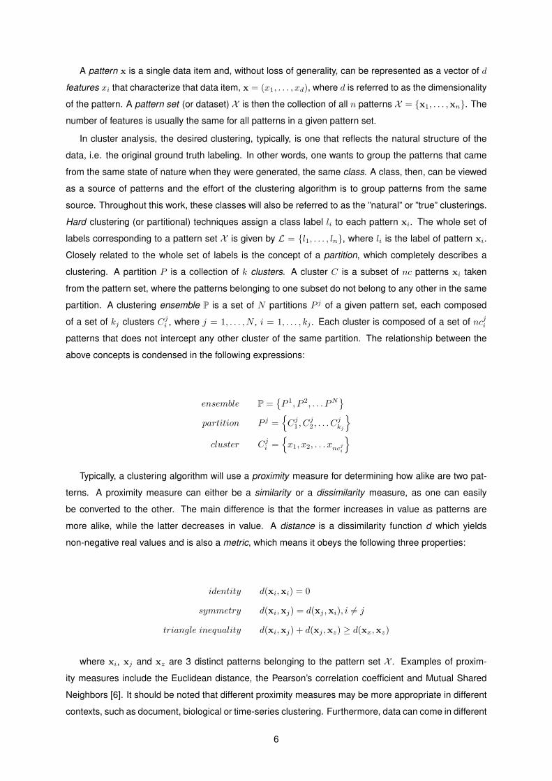
A pattern x is a single data item and, without loss of generality, can be represented as a vector of d
features xi that characterize that data item, x = (x1, . . . , xd), where d is referred to as the dimensionality
of the pattern. A pattern set (or dataset) X is then the collection of all n patterns X = {x1, . . . ,xn}. The
number of features is usually the same for all patterns in a given pattern set.
In cluster analysis, the desired clustering, typically, is one that reflects the natural structure of the
data, i.e. the original ground truth labeling. In other words, one wants to group the patterns that came
from the same state of nature when they were generated, the same class. A class, then, can be viewed
as a source of patterns and the effort of the clustering algorithm is to group patterns from the same
source. Throughout this work, these classes will also be referred to as the ”natural” or ”true” clusterings.
Hard clustering (or partitional) techniques assign a class label li to each pattern xi. The whole set of
labels corresponding to a pattern set X is given by L = {l1, . . . , ln}, where li is the label of pattern xi.
Closely related to the whole set of labels is the concept of a partition, which completely describes a
clustering. A partition P is a collection of k clusters. A cluster C is a subset of nc patterns xi taken
from the pattern set, where the patterns belonging to one subset do not belong to any other in the same
partition. A clustering ensemble P is a set of N partitions P j of a given pattern set, each composed
of a set of kj clusters Cji , where j = 1, . . . , N , i = 1, . . . , kj . Each cluster is composed of a set of ncjipatterns that does not intercept any other cluster of the same partition. The relationship between the
above concepts is condensed in the following expressions:
ensemble P ={P 1, P 2, . . . PN
}partition P j =
{Cj1 , C
j2 , . . . C
jkj
}cluster Cji =
{x1, x2, . . . xncji
}Typically, a clustering algorithm will use a proximity measure for determining how alike are two pat-
terns. A proximity measure can either be a similarity or a dissimilarity measure, as one can easily
be converted to the other. The main difference is that the former increases in value as patterns are
more alike, while the latter decreases in value. A distance is a dissimilarity function d which yields
non-negative real values and is also a metric, which means it obeys the following three properties:
identity d(xi,xi) = 0
symmetry d(xi,xj) = d(xj ,xi), i 6= j
triangle inequality d(xi,xj) + d(xj ,xz) ≥ d(xx,xz)
where xi, xj and xz are 3 distinct patterns belonging to the pattern set X . Examples of proxim-
ity measures include the Euclidean distance, the Pearson’s correlation coefficient and Mutual Shared
Neighbors [6]. It should be noted that different proximity measures may be more appropriate in different
contexts, such as document, biological or time-series clustering. Furthermore, data can come in different
6

types such as numerical (discrete or continuous) or categorical (binary or multinomial) attributes. The
researcher should take these factors into account as different proximity measures are more appropriate
for some type or even heterogeneous type data.
An introduction of clustering would be incomplete without a discussion on how good is a partition
after clustering. Several validity measures exist and they can placed in two main categories [7]. Exter-
nal measures use a priori information about the data to evaluate the clustering against some external
structure. An application of an external measure could be to test how accurate a clustering algorithm
is for a particular dataset by matching the output partition against the ground truth. The Consistency
Index [8] and the H-index [9] are examples of such measures that will be used in this work. Both of them
are based on giving a score to each pair of clusters from two different partitions and then choosing the
pairs that produce the best overall score. Internal measures, on the other hand, determine the quality
of the clustering without the use of external information about the data. The Davies-Bouldin index [10]
is such a measure. This index outputs a high score to partitions with high inter-cluster distance and low
intra-cluster distance, and vice versa.
2.3 Characteristics of clustering techniques
Clustering algorithms may be categorized and described according to different properties. For the sake
of completeness, a brief discussion of some of their properties will be layed out in this section.
It is common to organize cluster algorithms into two distinct types: partitional and hierarchical. A
partitional algorithm, such as K-Means, is a hard clustering algorithm that will output a partiton where
each pattern belongs exclusively to one cluster. A hierarchical algorithm produces a tree-based data
structure called dendrogram. A dendrogram contains different partitions at different levels of the tree
which means that the user can easily change the desired number of clusters by simply traversing the
different levels. This is an advantage over a partitional algorithm since a user can analyze different par-
titions with different numbers of clusters without having to rerun the algorithm. Hierarchical algorithms
can be further split into two approaches: bottom-up (or agglomerative) and top-down (or divisive). The
former starts with all patterns as distinct clusters and will group them together according to some dis-
similarity measure, building the dendrogram from the ground up; examples of algorithms that take this
approach are Single-Link and Average-Link. The latter will start will all patterns in the same cluster and
continuously split it until all patterns are separated, building the dendrogram from the top level to the
bottom; this approach is taken by the Principal Directon Divisive Partitioning [11] and Bisecting K-Means
[12] algorithms.
Another characteristic relates to how algorithms use the features for computing similarities. If all
features are used simultaneously the algorithm is called polithetic, e.g. K-Means. Otherwise, if the
features are used sequentially, it is called monothetic, e.g. [13].
Contrasting with hard clustering algorithms, are the fuzzy algorithms. A fuzzy algorithm will attribute
to each pattern a degree of membership to each cluster. A partition can still be extracted from this
output by choosing, for each pattern, the cluster with higher degree of membership. An example of a
7

fuzzy algorithm is the Fuzzy C-Means [14].
Another characteristic is an algorithm’s stochasticity. A stochastic algorithm uses a probabilistic
process at some point in the algorithm, possibly yielding different results in each run. As an example,
the K-Means algorithm typically picks the initialization centroids randomly. A deterministic algorithm, on
the other hand, will always produce the same result for a given input, e.g. Single-Link.
Finally, the last characteristic discussed is how an algorithm processes the input data. An algorithm
is said to be incremental if it processes the input incrementally, i.e. taking part of the data, processing
it and then doing the same for the remaining parts, e.g. PEGASUS [15]. A non-incremental algorithm,
on the other hand, will process the whole input in each run, e.g. K-Means. This discussion is specially
relevant when considering large datasets that may not fit in memory or whose processing would take
too long for a single run and is therefore done in parallel.
2.4 K-Means
One of the most famous non-optimal solutions for the problem of partitional clustering is the K-Means
algorithm [16]. The K-Means algorithm uses K centroid representatives, ck, for K clusters. Patterns are
assigned to a cluster such that the squared error (or, more accurately, squared dissimilarity measure)
between the cluster representatives and the patterns is minimized. In essence, K-Means is a solution
(although not necessarily an optimal one) to an optimization problem having the Sum of Squared Errors
as its objective function, which is known to be a computationally NP hard problem [2]. It can be mathe-
matically demonstrated that the optimal representatives for the clusters are the means of the patterns of
each cluster [7]. K-Means, then, minimizes the following expression, where the proximity measure used
is the Euclidean distance:
K∑k=1
∑xi∈Ck
‖xi − ck‖2 (2.1)
K-Means needs two initialization parameters: the number of clusters and the centroid initializations.
It starts by assigning each pattern to its closer cluster based on the cluster’s centroid. This is called
the labeling step since one usually uses cluster labels for this assignment. The centroids are then
recomputed based on this assignment, in the update step. The new centroids are the mean of all the
patterns belonging to the clusters, hence the name of the algorithm. These two steps are executed
iteratively until a stopping condition is met, usually the number of iterations, a convergence criteria or
both. The initial centroids are usually chosen randomly, but other schemes exist to improve the overall
accuracy of the algorithm, e.g. K-Means++ [17]. There are also methods to automatically choose the
number of clusters [7].
The proximity measure used is typically the Euclidean distance. This tends to produce hyperspherical
clusters [3]. Still, according to [2], other measures have been used such as the L1 norm, Mahalanobis
distance, as well as the cosine similarity [7]. The choice of similarity measure must be made carefully
8

as it may not guarantee that the algorithm will converge.
A detail of implementation is what to do with clusters that have no patterns assigned to them. One
approach to this situation is to drop the empty clusters in further iterations. However, allowing the
existence of empty clusters or dropping empty clusters is undesirable since the number of clusters is
an input parameter and it is expected that the output contains the specified number of clusters. Other
approaches exist dealing with this problem, such as equaling the centroid of an empty cluster to the
pattern furthest away from its assigned centroid or reusing the old centroids as in [18].
K-Means is a simple algorithm with reduced complexity O(ntk), where n is the number of patterns in
the pattern set, k is the number of clusters and t is the number of iterations that it executes. Accordingly,
K-Means is often used as a foundational step of more complex and robust algorithms, such as the EAC
algorithm.
As an example, the evolution and output of the K-means algorithm to the data presented in Fig. 2.1
is represented in Fig. 2.2. The algorithm was executed with 3 random centroids.
4.0 4.5 5.0 5.5 6.0 6.5 7.0 7.5 8.0First feature
2.0
2.5
3.0
3.5
4.0
4.5
Seco
nd fe
ature
K-Means clustering, iter=1
4.0 4.5 5.0 5.5 6.0 6.5 7.0 7.5 8.0First feature
2.0
2.5
3.0
3.5
4.0
4.5
Seco
nd fe
ature
K-Means clustering, iter=2
4.0 4.5 5.0 5.5 6.0 6.5 7.0 7.5 8.0First feature
2.0
2.5
3.0
3.5
4.0
4.5
Seco
nd fe
ature
K-Means clustering, iter=3
4.0 4.5 5.0 5.5 6.0 6.5 7.0 7.5 8.0First feature
2.0
2.5
3.0
3.5
4.0
4.5
Seco
nd fe
ature
K-Means clustering, converged
Figure 2.2: The output labels of the K-Means algorithm with the number of clusters (input parameter)set to 3. The different plots show the centroids (squares) evolution on each iteration. Between iteration3 and the converged state 2 more iterations were executed.
Even with the correct number of clusters, the clustering results do not match 100% the natural clus-
ters. The accuracy relative to the natural clusters of Fig. 2.1b is 88% as measured by the Consistency
Index (CI) [8]. In this example, the problem is the two overlapping clusters. It is hard for an algorithm to
9

discriminate between two clusters when they have similar patterns. When no prior information about the
dataset is given, the number of clusters can be hard to discover. This is why, when available, a domain
expert may provide valuable insight on tuning the initialization parameters.
2.5 Single-Link
Single-Link [19] is one of the most popular hierarchical agglomerative clustering (HAC) algorithms. HAC
algorithms operate over a pair-wise dissimilarity matrix and output a dendrogram (e.g. Fig 2.4a). The
main steps of an agglomerative hierarchical clustering algorithm are the following [3]:
1. Create a pair-wise dissimilarity matrix of all patterns, where each pattern is a distinct cluster sin-
gleton;
2. Find the closest clusters, merge them and update the matrix to reflect this change. The rows and
columns of the two merged clusters are deleted and a new row and column are created to store
the new cluster.
3. Stop if all patterns belong to a single cluster, otherwise continue to step 2.
The algorithm stops when n− 1 merges have been performed, which is when all patterns have been
connected in the same cluster. Just like in the K-Means algorithm, different similarity measures can be
used between pairs of objects.
The proximity measure between clusters in the second step distinguishes between the different HAC
linkage algorithms, such as Single-Link , Average-Link, Complete-Link, among others. In Single-Link
(SL), the proximity between any two clusters is the the dissimilarity between their closest patterns. On
the other hand, in Complete-Link, it is the proximity between their most distant patterns and, in Average-
Link, is the proximity between the average point of each cluster. In SL, because the algorithm connects
first clusters that are more similar, it naturally gives more importance to regions of higher density [7].
The total time complexity of a naive implementation is O(n3) since it performs a O(n2) search in step
two and it does it n − 1 times. Over time, more efficient implementations have been proposed, such
as SLINK [20]. SLINK needs no working copy of the O(n2) pair-wise similarity matrix (if the original
can be modified), has a working memory of O(n2) and time complexity of O(n2). This increase in
performance comes from the observation that the O(n2) search can be transformed in a O(n) search
at the expense of keeping two arrays of length n that will store the most similar cluster for each pattern
and the corresponding similarity measure. This way, to find the two closest clusters, the algorithm will
not search the entire similarity matrix, but only the new similarity array since this array keeps the closest
cluster of each cluster. Naturally these arrays must be updated upon a cluster merge.
An interesting property of the SL algorithm is its equivalence with a Minimum Spanning Tree (MST),
an observation first made by [21]. In graph theory, a MST is a tree that connects all vertices together
while minimizing the sum of all the distance between them. An example of a graph and its corresponding
MST can be seen in Fig. 2.3. In this context, the edges of the MST are the distances between the
10

patterns and the vertices are the patterns themselves. A MST contains all the information necessary to
build a Single-Link dendrogram. To walk down through the levels of the dendrogram from the MST, one
cuts the least similar edges. Furthermore, this approach can be used to apply Single-Link clustering
to graphs-encoded problems in a straight-forward way. Furthermore, the performance properties of this
method are roughly the same as SLINK [22].
The true advantage of using a MST based approach comes when the number of edges (similarities)
m of the MST is less than n(n−1)2 , where n is the number of nodes (patterns) [23]. This is because SLINK
works over a inter pattern similarity matrix, meaning that the similarity between every pair of patterns
must be explicitly represented. The minimum number of similarities is n(n−1)2 , which is equivalent to the
upper or lower half triangular matrices of the similarity matrix. The MST, on the other hand, works over
a graph that may or may not have edges between every pair of nodes. Fast MST algorithms have a time
complexity of O(m log n), which is a significant improvement over O(n2) when m << n(n−1)2 .
(a) Example of a graph. (b) MST of the graph to the left.
Figure 2.3: The above figures show an example of a graph (left) and its corresponding Minimum Span-ning Tree (right). The circles are vertices and the edges are the lines linking the vertices.
An example of a Single-Link dendrogram and resulting cluster can be observed in Fig. 2.4. The
dendrogram in Fig. 2.4a has been truncated to 25 clusters in the bottom level for the sake of readability.
The clustering presented on Fig. 2.4b is the result of cutting the dendrogram such that only 3 clusters
exist (the number of classes). The accuracy, as measured by the CI, is of 58%.
4122 14 1544(45)11713110698 60(2)109108134135118(2)(2)11462(2)1196410059 85(37)(14)(3)(5)(6)(7)102(2)Clusters
0.0
0.2
0.4
0.6
0.8
1.0
1.2
1.4
1.6
Sim
ilarit
y be
twee
n cl
uste
rs
Single-Link dendrogram
(a) Single-Link dendrogram truncated to 25 clustersin the bottom level.
4.0 4.5 5.0 5.5 6.0 6.5 7.0 7.5 8.0First feature
2.0
2.5
3.0
3.5
4.0
4.5
Seco
nd fe
ature
Single-Link clustering
(b) Clustering with 3 clusters.
Figure 2.4: The above plots show the dendrogram and a possible clustering taken from a Single-Link runover the Iris dataset. Fig. 2.4b was obtained by performing a cut on a level that would yield a partition of3 clusters.
11

2.6 Ensemble Clustering
The underlying idea behind ensemble clustering is to take a collection of partitions, a clustering ensem-
ble, and combine it into a single partition. There are several motivations for ensemble clustering. Data
from real world problems appear in different configurations regarding shape, cardinality, dimensionality,
sparsity, etc. Different clustering algorithms are appropriate for different data configurations, e.g. K-
Means tends to group patterns in hyperspheres [3] so it is more appropriate for data whose structure
is formed by hypershere like clusters. If the true structure of the data at hand is heterogeneous in its
configuration, a single clustering algorithm might perform well for some part of the data while other per-
forms better for some other part. Since different partitions are used, one can use a mix of algorithms
to address different properties of the data such that the combination is more robust to noise and out-
liers [24] and the final clustering has a better quality [7]. Even using several partitions from different
initializations of the same algorithm may also allow retrieving complex shaped structures from otherwise
simple methods. Ensemble clustering can also be useful in situations where one does not have direct
access to all the features of a given dataset but can have access to partitions from different subsets and
later combining with an ensemble algorithm. Furthermore, the generation of the clustering ensemble
can be parallelized and distributed since each partition is independent from every other partition.
A clustering ensemble, according to [25], can be produced from (1) different data representations,
e.g. choice of preprocessing, feature selection and extraction, sampling; or (2) different partitions of the
data, e.g. output of different algorithms, varying the initialization parameters on the same algorithm.
Ensemble clustering algorithms can take three main distinct approaches [7]: based on pair-wise sim-
ilarities, probabilistic or direct. EAC [25] and CSPA [26] are examples of pair-wise similarity based ap-
proach, where the algorithms use a co-associations matrix. The MMCE [24] and BCE [27] are examples
of a probabilistic approach. This approach will be further clarified when the EAC algorithm is explained.
HGPA [26], MCLA [26] and bagging [28] are examples of a direct approach to combining the ensemble
clusterings, where the algorithms work directly with the labels without creating a co-association matrix.
A detailed and thorough review of the similarity measures that can be used on with clustering ensembles
and the state of the art algorithms can be consulted in [7].
2.7 Evidence Accumulation Clustering
2.7.1 Overview
The goal of EAC is to find an optimal partition P ∗ containing k∗ clusters, from the clustering ensemble
P. The optimal partition should have the following properties [25]:
• Consistency with the clustering ensemble;
• Robustness to small variations in the ensemble; and,
• Goodness of fit with ground truth information, when available.
12

Ground truth is the true labels of each sample of the dataset, when such exists, and is used for
validation purposes. Since EAC is an unsupervised method, this typically will not be available. EAC
makes no assumption on the number of clusters in each data partition. Its approach is divided in 3
steps:
1. Production of a clustering ensemble P (the evidence);
2. Combination of the ensemble into a co-association matrix;
3. Recovery of the natural clusters of the data.
In the first step, a clustering ensemble is produced. Within the context of EAC, it is of interest to
have variety in the ensemble with the intention of better capturing the underlying structure of the data.
One such parameter to measure that variety is the number of clusters in the partitions of the ensemble.
Typically, the number of clusters in each partition is drawn from an interval [Kmin,Kmax] with uniform
probability. This influences other properties of other parts of the algorithm such as the sparsity of the
co-association matrix as will become clearer in future chapters. Reviewing the literature [29, 25, 30, 31],
it is clear the ensemble is usually produced by random initialization of K-Means (specifying only the
number of centroids within the above interval). Still, other clustering algorithms have been used for the
production of the ensemble [32] such as Single-Link, Average-Link and CLARANS.
The ensemble of partitions is combined in the second step, where a non-linear transformation turns
the ensemble into a co-association matrix [25], i.e. a matrix C where each of its elements nij is the
association value between the pattern pair (i, j). The association between any pair of patterns is given
by the number of times those two patterns appear clustered together in any cluster of any partition of
the ensemble, i.e. the number of co-occurrences in the same cluster. The rationale is that pairs that
are frequently clustered together are more likely to be representative of a true link between the patterns
[29], revealing the underlying structure of the data. In other words, a high association nij means it is
more likely that patterns i and j belong to the same class. The construction of the co-association matrix
is at the very core of this method.
The co-association matrix itself is not the output of EAC. Instead, it is used as input to other methods
to obtain the final partition. The co-association between any two patterns can be interpreted as a
similarity measure. Thus, since this matrix is a similarity matrix it’s appropriate to use algorithms that
take this type of matrices as input, e.g. K-Medoids or hierarchical algorithms such as Single-Link or
Average-Link, to name a few. Typically, algorithms use a distance as the dissimilarity, which means that
they minimize the distance to obtain the highest similarity between objects. However, a low value on
the co-association matrix translates in a low similarity between a pair of objects, which means that the
co-association matrix requires prior transformation for accurate clustering results, e.g. replace every
similarity value nij between every pair of object (i, j) by max{C} − nij .
Although any algorithm can be used, the final clustering is usually done using SL or AL. Each of
these algorithms will take as input the transformed co-association matrix as the dissimilarity matrix.
Furthermore, not knowing the ”natural” number of clusters one can use the lifetime criteria. The k-
cluster lifetime is defined by Fred and Jain [25] as the range of threshold values on the dendrogram that
13

lead to the identification of k clusters. The lifetime criteria chooses the longest lifetime as the threshold
interval where a cut in the dendrogram should be made so as to produce a partition. In other words,
the number of clusters k should be such that it maximizes the cost of cutting the dendrogram from k− 1
clusters to k.
Related work to EAC has been developed. The Weighted EAC (WEAC) algorithm [32] and a study
on the sparsity of the co-association matrix [33] should be mentioned. The latter is discussed in more
depth in chapter 3. The former introduces the novelty of having weights associated to each partition
such that good quality partitions are more relevant than their counterparts. These weights are based on
internal validity measures. Weighing the partitions in terms of quality has shown to improve the original
algorithm, accuracy wise.
EAC has been used with success in several areas. To name a few, it was used for the automatic
identification of chronic lymphocyt leukemia [34], for the unsupervised analysis of ECG-based biometric
database to highlight natural groups and gain further insight [31] and as a solution to the problem of
clustering of contour images (from hardware tools) [30].
14

Chapter 3
State of the art
Scalability of EAC to large datasets is the concern of this work and, because of that, this chapter starts
by reviewing what has been done in terms of scaling EAC in section 3.1. EAC is a method of three parts
and this dissertation is concerned with the scalability of the whole algorithm which means that each step
must be optimized. Scaling an algorithm means one has to take into account both speed of execution
and memory requirements. Increasing speed can be attained with either faster algorithms and/or faster
computation of existing algorithms. This chapter reflects research done within both approaches.
Although research on the application of EAC to large datasets has not been pursued before, cluster
analysis of large datasets has. Since EAC uses traditional clustering algorithms (e.g. K-Means, Single-
Link) in its approach, it is useful to understand how scalable the individual algorithms are as they will have
a big impact in the scalability of EAC. Furthermore, valuable insights may be taken from the techniques
used in the scalability of other algorithms. To this end, section 3.2 presents a brief review on cluster
analysis of large datasets, with a focus on parallelization with GPUs. Furthermore, it offers a more
detailed description of a GPU parallel version of K-Means and an approach for parallelizing Single-Link
with the GPU.
An alternative approach on clustering for scaling with faster algorithms, the still young field of quan-
tum clustering, was reviewed in section 3.3. This line of research was taken mostly with the first step of
EAC in mind.
3.1 Scalability of EAC
The quadratic space and time complexity of processing the n×n co-association matrix is an obstacle to
an efficient scaling of EAC. Two approaches have been proposed to address this obstacle: one dealing
with reducing the co-association matrix by considering only the distances of patterns to their p neighbors
and the other by using a sparse co-association matrix and maximizing its sparsity.
15

3.1.1 p neighbors approach
The first approach, [25], proposes an alternative n × p co-association matrix, where only the p nearest
neighbors of each pattern are considered in the evidence combination step. This comes at the cost of
having to keep track of the neighbors of each pattern in a separate data structure of O(np) memory
complexity and also of pre-computing the p neighbors, which has a time complexity of O(n2) to compute
the proximity measure from each pattern to every other pattern. The quadratic space complexity of
the co-association matrix is then transformed to O(2np): O(np) for the actual co-association matrix
and O(np) for keeping track of the neighbors. Since usually one has p < n2 (value for which both this
approach and the original n × p matrix would take the same space), the cost of storing the extra data
structure is lower than that of storing an n×n matrix, e.g. for a dataset with 106 patterns and p =√106 (a
value much higher than the 20 neighbors used in [25]), the total memory required for the co-association
matrix would decrease from 3725.29GB to 7.45GB (0.18% of the memory occupied by the complete
matrix).
3.1.2 Increased sparsity approach
The second approach, presented in [33], exploits the sparse nature of the co-association matrix. The
co-association matrix is symmetric and with a varying degree of sparsity. The former property translates
in the ability of storing only the upper triangular of the matrix without any loss on the quality of the
results. The latter property is further studied with regards to its relationship with the minimum Kmin and
maximum Kmax number of clusters in the partitions of the input ensemble. The core of this approach is
to only store the non-zero values of the upper triangular of the co-association matrix. The authors study
3 models for the choice of these parameters:
• choice of Kmin based on the minimum number of gaussians in a gaussian mixture decomposition
of the data;
• based on the square root of the number of patterns ({Kmin,Kmax} = {√n2 ,√n});
• or based on a linear transformation of the number of patterns ({Kmin,Kmax} = { nA ,nB }, A < B).
where A and B are two suitable constants chosen by the researcher. The study compared the impact
of each model in the sparsity of the co-association matrix (and, thus, the space complexity) and in the
relative accuracy of the final clusterings. Both theoretical predictions and results revealed that the linear
model produces the highest sparsity in the co-association matrix, under a dataset consisting of a mixture
of Gaussians. Furthermore, it is true for both linear and square root models that the sparsity increases
as the number of samples increases.
For real datasets, the performance of the three models became increasingly similar with the increase
of the cardinality of the problem. It was found that the chosen granularity of the input partitions (Kmin) is
the variable with most impact, affecting both accuracy and sparsity. The authors reported this technique
has linear space and time complexity on benchmark data.
16
The number of samples of the datasets analysed in [33] was under 104. Furthermore, it should
be noted that the remarks concerning the sparsity of the co-association matrix in the aforementioned
study refer to the number of non-zero elements in the matrix and does not take into account extra data
structures that accompany real sparse matrices implementations.
3.2 Clustering with large datasets
When large datasets, and big data, is in discussion, two perspectives should be taken into account [7].
The first deals with the applications where data is too large to be stored efficiently. This is the problem
that streaming algorithms such as LOCALSEARCH [35] try to solve by analyzing data as it is produced,
close to real-time processing. The other perspective is data that is actually stored for later processing
which is the perspective relevant to the present work and will be further discussed below.
The flow of clustering algorithms typically involves some initialization step (e.g. choosing the number
of centroids in K-Means) followed by an iterative process until some stopping criteria is met, where each
iteration updates the clustering of the data [7]. In light of this, to speed up and/or scale up an algorithm,
three approaches are available: (1) reduce the number of iterations, (2) reduce the number of patterns
and/or features to process or (3) parallelizing and distributing the computation. The solutions for each of
these approaches are, respectively, one-pass algorithms (e.g. CLARANS [36], BIRCH [37], CURE [38]),
randomized techniques that reduce the input space complexity (e.g. PCA, CX/CUR [39]) and parallel
algorithms (parallel K-Means [40], parallel spectral clustering [41]).
Parallelization can be attained by adapting algorithms to multi core CPU, GPU, distributed over sev-
eral machines (a cluster ) or a combination of the former, e.g. parallel and distributed processing using
GPU in a cluster of hybrid workstations. Each approach has its advantages and disadvantages. The
CPU approach has access to a larger memory but the number of computation units is reduced when
compared with the GPU or cluster approach. Furthermore, CPUs have advanced techniques such as
branch prediction, multiple level caching and out of order execution - techniques for optimized sequen-
tial computation. GPU have hundreds or thousands of computing units but typically the available device
memory is reduced which entails an increased overhead of memory transfer between host (worksta-
tion) and device (GPU) for computation of large datasets. In addition, it is harder to scale the above
solutions for even bigger datasets. On the other hand, GPUs can be found on a large variety of com-
puting platforms, from mobile devices to workstations and datacenters. A cluster offers a parallelized
and distributed solution, which is easier to scale. According to [7], the two algorithmic approaches for
cluster solutions are (1) memory-based, where the problem data fits in the main memory of the ma-
chines of the cluster and each machine loads part of the data; or (2) disk-based, comprising the widely
used MapReduce framework capable of processing massive amounts of data in a distributed way. The
main disadvantage is that there is a high communication and memory I/O cost to pay. Communication is
usually done over the network with TCP/IP, which is several orders of magnitude slower than the direct
access of the CPU or GPU to memory (host or device).
The present work is oriented towards GPU based parallelization, since GPUs are an easily accessible
17

commodity and the goals of the dissertation are oriented towards computation on a single machine.
Taking that into consideration, this section reviews a GPU parallel version of the K-Means algorithm and
goes on to describe a GPU parallel approach for performing Single-Link clustering. For an overview of
General Purpose computing in GPUs (GPGPU), the reader is referred to Appendix A.
3.2.1 Parallel K-Means
K-Means is an obvious candidate to generate the ensemble of the first step of EAC because it uses dif-
ferent initializations and parameters and due to its simplicity. Besides, K-Means is a very good candidate
for parallelization. Still, other algorithms can be used to produce ensembles.
Several parallel implementations of this algorithm for the GPU exist [42, 43, 44, 45, 46] and all report
significant speed-ups relative to their sequential counterparts in certain conditions, usually after the input
dataset goes above a certain cardinality, dimensionality or number of clusters threshold. The first step
is inherently parallel as the computation of the label of the i-th pattern is not dependent on any other
pattern, but only on the centroids. Two approaches to parallelize this step on the GPU are possible,
a centroid-centric or a data-centric [42]. In the former each thread is responsible for a centroid and
will compute the distance from its centroid to every pattern. These distances must be stored and, in
the end, the patterns are assigned to the closest centroid. In the latter, each thread will compute the
distance from one or more data points to every centroid and determines to which centroid they are
closest. This strategy has the advantage of using less memory since it does not need to store all the
pair-wise distances to perform the labeling - it only needs to store the best distance for each pattern.
According to [42], the former approach is suitable for devices with a low number of cores so as to stream
the data to each one, while the latter is better suited to devices with more cores.
The approach taken in [40] only parallelizes the labeling stage and takes a data-centric approach
to the problem. Each thread computes the distance from a set of data points to every centroid and
determines the labels. The remaining steps are performed by the host CPU. This study reported speed-
ups up to 14, for input datasets of 500 000 points. Furthermore, it should be noted that the speed up was
measured against a sequential version with all C++ compiler optimizations turned on, including vector
operations (which, by themselves, are a way of parallelizing computation). The parallelized algorithm’s
flow can be observed in Figure 3.1.
The implementation of Zechner and Granitzer [40] uses one thread per data point. Each centroid
is transfered to shared memory and each thread will compute the distance from its data point to the
centroid. Moreover, the data point is fetched from global memory in a coalesced manner.
It should be noted that the literature reports that the performance of K-Means using Dynamic Paral-
lelism is slightly worse than its standard GPU counterpart [47].
3.2.2 Parallel Single-Link Clustering
Single-Link (SL) is an important step in the EAC chain. Given the new similarity metric (how many times
a pair of patterns are clustered together in the ensemble), SL provides an intuitive way of obtaining
18

Figure 3.1: Flow execution of the GPU parallel K-Means algorithm.
19

the final partition: patterns that are clustered together often in the ensemble should remain clustered
together in the final solution.
SL is not easily parallelized since a new cluster generated at each step may include the one gener-
ated in the previous iteration. The most parallelizable part is the computation of the pair-wise similarity
matrix, which is only useful if the input is raw data instead of a similarity matrix as in the case of EAC.
The relationship between SL and the Minimum Spanning Tree, explained in chapter 2, is the key to par-
allelize it. If one takes this approach for solving the SL problem, it becomes easier to parallelize it since
parallel MST algorithms are abundant in literature [48, 49, 50]. The same approach for extracting the
final clustering in EAC was used in [29].
Algorithm for finding Minimum Spanning Trees
There are several algorithms for computing an MST. The most famous are Kruskal [51], Prim [52] and
Boruvka [53]. Boruvka’s algorithm is also known as Sollin’s algorithm. The first two are mostly sequen-
tial, while the latter has the highest potential for parallelization, specially in the first iterations. As such,
even though GPU parallel variants of Kruskal’s [49] and Prim’s [54] algorithms exist, the focus will be on
Boruvka’s.
Several parallel implementations of this algorithm for the GPU exist, e.g. [48], [55] and [50]. Da Silva
Sousa et al. [50] provides a more in-depth review over the current state of the art of MST solvers for
the GPU and proposes an algorithm reported to be the fastest. This section will review the algorithm
proposed in [50], referred to as Sousa2015 from henceforth.
Since this algorithm operates over graphs, relevant graph notation is introduced here. In graph theory,
a graph G = (V,E) is composed by a set of vertices V and a set of edges E connecting those vertices.
Furthermore, if G is a connected graph, then there is a path between any s, t ∈ V . An example of a
graph can be observed in Fig. 2.3 of chapter 2, where the MST was first introduced. A |V | × |V | matrix
can fully represent a graph if one takes each element (i, j) of the matrix to be the weight of the edge
connecting vertices i and j. Typically, a graphs is not fully connected (vertices connected to all the other
vertices), which means that the matrix is often sparse.
CSR format
Sousa2015 takes in a graph as input, represented in the CSR format (a format used for sparse matrices).
This representation is equivalent to having a square matrixG with zeroed diagonal where the gij element
of the matrix is the weight of the link connecting the node i with the node j. This format is represented
in Fig. 3.2. It requires three arrays to fully describe the graph:
• a data array containing all the non-zero values, where values from the same row appear sequen-
tially from left to right and top to bottom, i.e. in row-major order, e.g. if the first row has 20 non-zero
values, then the first 20 elements from this array belong to the first row;
• an indices array of the same size as data containing the column index of each non-zero value;
20

• an indptr array of the size of the number of rows containing a pointer to the first element in the
data and indices arrays that belongs to each row, e.g. if the i− th element (row) of indptr is k and
it has 10 values, then all the elements from k to k + 10 in data belong to the i− th row.
0 2 3
6 3 9 2 1
1 2 0 1 26 3
9
2 1
0 1 2
0
1
2
0 1 2
data
indices
indptr
0 1 2 3 4
Figure 3.2: Correspondence between a sparse matrix and its CSR counterpart.
Within the algorithm’s context, these three arrays are denominated as first edge, destination and
weight, respectively. There change in denomination is for making their purposes clearer. Although these
three arrays can completely describe a graph, the algorithm uses an extra array outdegree that stores
the number of non-zero values of each row and can be deduced from the first edge array.
The length and purpose of each of these arrays are:
• first edge is an array of size |V |, where the i-th element points to the first edge corresponding to
the i-th vertex.
• outdegree is an array of size |V |, where the i-th element contains the number of edges attached to
the i-th vertex.
• destination is an array of size |E|, where the j-th element points to the destination vertex of the j-th
edge.
• weight is an array of size |E|, where the j-th element contains the weight of the j-th edge.
|V | is the number of vertices and |E| is the number of edges. The number of edges is duplicated
to cover both directions, since the algorithm works with undirected graphs. This basically means that
instead of using the the upper (or lower) triangular matrix (which can also completely describe the graph),
it uses a complete matrix resulting in double redundancy of each edge. The edges in the destination
array are grouped together by the vertex they originate from, e.g. if edge j is the first edge of vertex
i and this vertex has 3 edges, then edges {j, j + 1, j + 2} are the outgoing edges of vertex i and are
stored sequentially in the destination array.
Steps of the algorithm
Within the context of the algorithm the id of a vertex is its index in the first edge array, the color repre-
sents a component and is the id of the component representative and the successor of a vertex is the
destination vertex of one of its edges. One should keep in mind this is a parallel algorithm and each
of its steps is computed concurrently. Except for the exclusive prefix sum, each thread processes a
21

single vertex and each computation is usually independent. In some steps, however, threads need to
access the same resource and it is important the state of the resource does not change in the middle
of the operation that accesses it. In these cases, atomic operations (operation that are guaranteed to
be isolated and, thus, not interruptible) are used. The algorithm’s flow is presented in Figure 3.3 and its
main steps are explained below.
1. Find minimum edge per vertex : select and store the minimum weighted edge for each vertex and
resolve same weight conflict by picking the edge with lower destination vertex id.
2. Remove mirrored edges: an edge is mirrored if the successor of its the destination vertex is the
origin vertex, e.g. if vertex 1 points to vertex 2 and vertex 2 points back to vertex 1. All mirrored
edges are removed from the selected edges in the first step. All edges that are not removed are
added to the resulting MST.
3. Initialize and propagate colors: this step is responsible for identifying connected components so
the graph may be contracted. Each connected component will be a super-vertex in the contracted
graph, which means it will be a single vertex representing a subgraph. Each vertex is initialized
with the same color of its successor’s id. If a vertex has no successor because that edge was
removed in the previous step, then it will be the representative vertex of the component and its
color is initialized with its own id. The colors are then propagated by setting each vertex’s color to
the color of its successor, until convergence.
4. Create new vertex ids: only the super-vertices will be propagated to the next iteration but they will
have new ids for building the new contracted graph. The new ids will range from 0 to s, where s
is the number of super-vertices. The vertices representing a super-vertex (component) will take
the new ids in increasing order according to their own ids in increasing order, e.g. vertex 2 is the
representative with lowest id so it will have the id 0 in the contracted graph. This step relied on the
exclusive scan operation, which is explained in section 3.2.2.
5. Count, assign, and insert new edges: the final step consists in building the contracted graph. The
algorithm will count the number of edges connecting each super-vertex to other super-vertices,
i.e. the connections between subgraphs. This is simply accomplished by selecting every edge
whose origin and destination colors are distinct. For each such edge the corresponding positions
of the origin and destination super-vertices in a new outdegree array are incremented with an
atomic operation. The new first edge array is obtained from performing an exclusive scan over
outdegree. The next step is to assign and insert edges in the contracted graph. Once again,
the algorithm will determine which edges will be in the contracted graph by checking the origin
and destination colors. A copy, called top edge, of the new first edge array will track of where to
insert the new edges. When an edge is assigned to a super-vertex it is inserted in the new weight
and destination arrays composing the contracted graph. The position of insertion is specified by
top edge and the algorithm increments top edge atomically so the next edge will not overwrite
the previous one. The increment is done with an atomic operation since multiple edges can be
22

assigned to the same super-vertex and the insertion of all edges is being done in parallel. It
should be noted that duplicated edges are not removed, i.e. several distinct connections between
two super-vertices can be kept, since the author considers that the benefit of doing so does not
outweigh the computational overhead.
Figure 3.3: Flow execution of Sousa2015.
It should be noted, however, that this algorithm does not support unconnected graphs, i.e., it is not
able to output a forest of MSTs. A solution to that problem is, on the step of building the flag array, only
mark a vertex if it is both the representative of its supervertex and has at least one neighbour.
23

Exclusive scan
The scan operation is one of the fundamental building blocks of parallel computing. Furthermore, two
of the steps of the Boruvka variant of [50] are performed with an exclusive scan where the operation is
a sum. To illustrate the functioning of the exclusive scan, let us consider the particular case where the
operation of the scan is the sum and the identity (the value for which the operation produces the same
output as the input) is naturally 0. An example of this operation is presented in Fig. 3.4.
Figure 3.4: Example of the exprefix sum operation.
The first element of the output will be the identity (if it were an inclusive scan, it would be the first
element itself). The second element is the sum between the first element of the input array and the
first element of the output array, etc. The nature of this algorithm seems highly sequential, since each
element of the output array depends on the previous one, but two main parallel versions can be found
in literature: Hillis and Steele [56] and Blelloch [57]. The two approaches focus on distinct efforts. The
former focuses on optimizing the number of steps [56], has a work complexity of O(nlogn) and a step
complexity of O(logn). The latter focuses on optimizing the amount of work done [57], has a work
complexity of O(n) and a step complexity of O(2logn). The focus of this dissertation will be on the
Blelloch’s algorithm. The reason for this is that the main objective is to deal with very large datasets
which guarantees that there will be more work to be done (operations on the data) than there will be
available computing resources (streaming processors in the GPU in this case). When there is more work
than processors, one wants to minimize the total amount of work. On the other hand, when there is more
processors than work, one wants to minimize the amount of steps of the algorithm as this translates in
the biggest increase in speed.
Blelloch’s algorithm is comprised by two main phases: the reduce phase (or up-sweep) and the
down-sweep phase. The algorithm is based on the concept of balanced binary trees [58], but it should
be noted that no such data structure is actually used. An in-depth explanation of this concept and how
it relates to the algorithm falls outside the scope of the present work and it is recommended that the
reader consult [58] or [57] for such details.
During the reduce phase (see Figure 3.5), the algorithm traverses the tree and computes partial
sums at the internal nodes of the tree. This operation is also known as a parallel reduction due to the
fact that the total sum is stored in the root node (last node) of the tree [58].
In the down-sweep phase (see Figure 3.6) the algorithm traverses back the tree. During the traversal,
and using the partial sums calculated in the reduce phase, it builds the scan in place (overwriting the
result of the reduce phase).
The computational complexity of this algorithm is higher than that of its sequential counterpart. The
24

Figure 3.5: Representation of the reduce phase of Blelloch’s algorithm [58]. d is the level of the tree andthe input array can be observed at d = 0.
Figure 3.6: Representation of the down-sweep phase of Blelloch’s algorithm [58]. d is the level of thetree.
25

sequential version has a O(n) computational complexity, since it only goes through the input array once
and performs exactly n additions. Blelloch’s algorithm, on the other hand, performs n − 1 additions in
the reduce phase and n − 1 in the down-sweep phase, but still keeps the linear work complexity of
the sequential version. Since it is a parallel algorithm and the computation will be distributed across
several processing units, its performance is significantly better. It should be noted that, as described,
the algorithm supports input arrays of a size that is a power of 2. However, Harris et al. [58] explains
how to overcome this limitation and also offers the description of an implementation for CUDA along with
hardware specific optimizations, which presented a speed-up as high as 6.
3.3 Quantum clustering
The field of quantum clustering has shown promising results regarding potential speed-ups in several
tasks over their classical counterparts. Currently, two major approaches for the concept of quantum
clustering were found in the literature: quantization of clustering methods to work in quantum computers
or algorithms inspired by quantum physics.
The former approach translates in converting algorithms to work partially or totally on a different
computing paradigm, with support of quantum circuits or quantum computers. Both Aımeur et al. [59]
and Lloyd et al. [60] show how the quantum paradigm can be used for speed-ups in machine learning
algorithms, with the possibility of obtaining exponential speed-ups. Many of these quantizations make
use of Groover’s database search algorithm [61], or a variant of it, e.g. Wiebe et al. [62]. Most literature
on this approach is also mostly theoretical, since the physical requirements still do not exist for testing
these methods. This approach can be seen as part of the bigger problem of quantum computing and
quantum information processing. An alternative to using real quantum systems would be to simulate
them. However, simulating quantum systems in classical computers is a very hard task by itself and
literature suggest that it is not feasible [63]. The quantization approach falls outside the scope of this
dissertation, but Wittek [64] offers a thorough review on the state of the art of machine learning in the
quantum paradigm.
The second approach is part of the wider field of Computational Intelligence. A study of the literature
reveals that it typically further divides itself into two categories [65]. One comprises the algorithms
based on the concept of the qubit, the quantum analogue of a classical bit with interesting properties
found in quantum objects. Several algorithms have been modeled after this concept, often also gathering
inspiration from evolutionary genetic algorithms, which were successfully applied in several areas:
• tackling the Knapsack problem as described in Han and Kim [66] and its improved version [67];
• solving the traveling salesman problem [68];
• two implementations of a Quantum K-Means algorithm [69, 70];
• a Quantum Artificial Bee Colony algorithm [71, 65];
26

• two approaches for Fuzzy C-Means (FCM), namely Quantum New Weighted Fuzzy C-Means
(QNW-FCM) [65] and Quantum Fuzzy C-Means (QFCM) [72, 65];
• a novel quantum inspired clustering technique based on manifold distance [73];
• a Quantum-inspired immune clonal clustering algorithm based on watershed [74].
The other approach models data as a quantum system and uses Schrodinger’s equation in some way.
Often, the data is modeled as a quantum system, where each pattern is a particle, and Schrodinger’s
equation is used to evolve the particle system into a solution. This has been applied in an optimiza-
tion problem for electromagnetics using a quantum particle swarm [75] and also on several clustering
algorithms:
• the Quantum Clustering [76] algorithm treats patterns as quantum particles whose potential is
computed with Schrodinger’s equation and the system is evolved with the Gradient Descent method;
• Dynamic Quantum Clustering [77] is a variation of Horn and Gottlieb [76] that uses Schrodinger’s
equation to evolve the system;
• a Fuzzy C-Means approach [78] based on Quantum Clustering [76];
• QPSO+FCM, a Fuzzy C-means [79] based on Quantum-behaved Particle Swarm Optimization
(QPSO) [80].
For more information on quantum inspired algorithms, the reader is referred to Manju and Nigam
[81] which offers a thorough survey on the state of the art of quantum inspired computation intelligence
algorithms. The following two sections contain a brief overview of the concept of the qubit and the de-
scription of an algorithm that uses this approach. Afterwards, an algorithm that follows the Schrodinger’s
equation approach is reviewed.
3.3.1 The quantum bit approach
The quantum bit
To understand the algorithms based on the concept of the qubit, it is useful to cast some insight about its
properties and functioning. This section has the purpose to provide a brief introduction to this topic. An
extended and in-depth review of this and related topics can be found in Lanzagorta and Uhlmann [82].
The qubit is a quantum object with certain quantum properties such as entanglement and superposition.
Within the context of the studied algorithm, the only property used is superposition. A qubit can have any
value between 0 and 1 (superposition property) until it is observed, which is when the system collapses
to either state. However, the probability with which the system collapses to either state may be different.
The superposition property or linear combination of states can be expressed [69] as
|ψ〉 = α|0〉+ β|1〉
27
where ψ is an arbitrary state vector and α, β are the the probability amplitude coefficients of basis
states |0〉 and |1〉, respectively. The Dirac bra ket notation is employed, where the ket |.〉 corresponds
to a column vector. The basis states correspond to the spin of the modeled particle (in this case, a
ferminion, e.g. electron). The coefficients are subjected to the following normalization:
|α|2 + |β|2 = 1
where |α|2, |β|2 are the probabilities of observing states [0] and [1], respectively, and α and β are
complex quantities that represent a qubit:
αβ
Moreover, a qubit string may be represented by:α1
β1
∣∣∣∣∣∣ α2
β2
∣∣∣∣∣∣ α3
β3
The probability of observing the state |000〉 will be |α1|2×|α2|2×|α3|2. To use this model for computing
purposes, black-box objects called oracles are used. Oracles are important to understand quantum
speed-ups. They can be understood as subroutines that cannot be usefully examined or as unknown
physical systems that perform a quantum operation on a qubit string [83] and with properties one would
like to estimate. Within the context of the present work an oracle is an abstraction for the programmer.
It is an object which can be called and changes state (which can be observed) as a consequence. For
the purpose of the following sections, the concept of the oracle is more related to oracles with internal
randomness [83] or, more simply, a probabilistic Turing machine, as in the case of [71].
Quantum K-Means
The Quantum K-Means (QK-Means) algorithm, as described in [69], is based on the classical K-Means
algorithm. It extends the basic K-Means with concepts from quantum mechanics (the qubit) and evolu-
tionary genetic algorithms.
Within the context of this algorithm, oracles contain strings of qubits and generate their own input by
observing the state of the qubits. After collapsing, the qubit value corresponds to a classical bit, with a
binary value.
Ideally, oracles would contain actual quantum systems or simulate them - this would correctly account
for the desirable quantum properties. As it stands, oracles are not quantum systems or even simulate
them and can be more appropriately described as random number generators. Each string of qubits
represents a number, so the number of qubits in each string will define its precision. The number of
strings chosen for the oracles depends on the number of clusters and dimensionality of the problem
(e.g. for 3 centroids of 2 dimensions, 6 strings will be used since 6 numbers are required). Each oracle
will represent a possible solution.
28

The algorithm has the following steps:
1. Initialize population of oracles
2. Collapse oracles
3. K-Means
4. Compute cluster fitness
5. Store
6. Quantum Rotation Gate
7. Collapse oracles
8. Quantum cross-over and mutation
9. Repeat 3-7 until generation (iteration) limit is reached
Initialize population of oracles The oracles are created in this step and all qubit coefficients are
initialized with 1√2, so that the system will observe either state of the qubit with equal probability. This
value is chosen taken into account the necessary normalization of the coefficients, as described in the
previous section.
Collapse oracles Collapsing the oracles implies making an observation of every qubit of each string
in all oracles. This is done by first choosing a coefficient to use (either can be used), e.g. α. Then, a
random value r between 0 and 1 is generated. If α ≥ r then the system collapses to [0], otherwise to [1].
K-Means In this step we convert the binary representation of the qubit strings to base 10 and use
those values as initial centroids for K-Means. For each oracle, classical K-Means is then executed until
it stabilizes or reaches the iteration limit. The solution centroids are returned to the oracles in binary
representation.
Compute cluster fitness Cluster fitness is computed using the Davies-Bouldin index for each oracle.
The score of each oracle is stored in the oracle itself.
Store The best scoring oracle is stored.
Quantum Rotation Gate So far, the algorithm consisted of the classical K-Means with a complex
random number generation for the centroids and complicated data structures, namely the oracles. This
is the step that fundamentally differs from the classical version. In this step, a quantum gate (in this
case a rotation gate) is applied to all oracles except the best one. The basic idea is to shift the qubit
coefficients of the least scoring oracles in the direction of the best scoring one. These oracles will have
a higher probability of collapsing into initial centroid values closer to the best solution so far. This way, in
29
future generations, the oracles do not initiate with the best centroids so far (which would not converge
into a better solution) but we they are close while still ensuring diversity (which is also a desired property
in the genetic computing paradigm). In other words, we look for better solutions than the one we got
before in each oracle while moving in the direction of the best we found so far.
The genetic operations of cross-over and mutation are both part of the genetic algorithms toolbox.
Literature suggests that this operations may not be required to produce variability in the population of
qubit strings [67]. The reason for this is that enough variability is produced with the use of the angle-
distance rotation method [67] in the quantum rotation operation, with a careful choice of the rotation
angle. Still, when used, the goal of these operations is to produce further variability into the population
of qubit strings.
3.3.2 Schrodinger’s equation approach
The other approach to clustering that gathers inspiration from quantum mechanical concepts is to use
the Schrodinger equation. The algorithm under study was created by Horn and Gottlieb [84] and was
later extended by Weinstein and Horn [77].
The first step in this methodology is to compute a probability density function of the input data. This
is done with a Parzen-window estimator in [85, 77]. The Parzen-window density estimation of the input
data is done by associating a Gaussian with each point, such that
ψ(x) =
N∑i=1
e−‖x−xi‖2
2σ2
where N is the total number of points in the dataset, σ is the variance and ψ is the probability density
estimation. ψ is chosen to be the wave function in Schrodinger’s equation. Further details can be found
in Weinstein and Horn [77], Horn and Gottlieb [85, 76].
With this information, one will compute the potential function V (x) that corresponds to the state of
minimum energy (ground state = eigenstate with minimum eigenvalue) [85], by solving the Schrodinger’s
equation in order of V (x):
V (x) = E +σ2
2 ∇2ψ
ψ= E − d
2+
1
2σ2ψ
N∑i=1
‖x− xi‖2 e−‖x−xi‖2
2σ2 (3.1)
And since the energy should be chosen such that ψ is the groundstate (i.e. eigenstate correspond-
ing to minimum eigenvalue) of the Hamiltonian operator associated with Schrodinger’s equation (not
represented above), the following is true
E = −minσ2
2 ∇2ψ
ψ(3.2)
From equations 3.1 and 3.2, V (x) can be computed. This potential function is related to the inverse of
30

a probability density function. Minima of the potential correspond to intervals in space where points are
together. So minima will naturally correspond to cluster centers [85]. However, it is very computationally
intensive to compute V (x) to the whole space, so the compututation of the potential function is only
done at the data points. This should not be problematic since clusters’ centers are generally close to the
data points themselves. Even so, the minima may not lie on the data points themselves. One method
to address this problem is to compute the potential on the input data and converge these points toward
some minima of the potential function. This is done with the gradient descent method in [85].
Another method [77] is to think of the input data as particles and use the Hamiltonian operator to
evolve the quantum system in the time-dependent Schrodinger’s equation. Given enough time steps,
the particles will converge to and oscillate around potential minima. This method makes the Dynamic
Quantum Clustering algorithm. The nature of the computations involved in this algorithm make it a good
candidate for parallelization techniques. Wittek [86] parallelized this algorithm to the GPU obtaining
speed-ups of up to two magnitudes relative to an optimized multicore CPU implementation.
31

Chapter 4
EAC for large datasets: proposed
solutions
The aim of this thesis is the optimization and scalability of EAC, with a focus for large datasets. EAC
is divided in three steps and each has to be considered for optimization. This chapter will present the
considered solutions for each step, which are also visually summarized in Fig. 4.1.
Figure 4.1: Diagram of proposed solution in each phase of EAC.
The first step is the gathering of evidence, i.e. generating an ensemble of partitions. The main
objective for the optimization of this step is speed. Using fast clustering methods for generating partitions
is an obvious solution, as is the optimization of particular algorithms aiming for the same objective. Since
each partition is independent from every other partition, parallel computing over a cluster of computing
units would result in a fast ensemble generation. Using either or any combination of these strategies will
guarantee a speed-up.
Initial research was under the field of quantum clustering. After this pursuit proved fruitless for being
slow, the focus of research shifted to parallel computing, more specifically a K-Means parallel version
within the GPGPU paradigm.
32

The second step is mostly bound by memory. The complete co-association matrix has a space
complexity of O(n2). Such complexity becomes prohibitive for big data, e.g. a dataset of 2×10⁶ patterns
will result in a complete co-association matrix of 14901 GB if values are stored in single precision floating-
point format. This problem is addressed by exploring the inherent sparse nature of the co-association
matrix.
The last step has to take into account both memory and speed requirements. The final clustering
must be able to produce good results and be fast while not exploding the already big space complexity
from the co-association matrix. The work in this last step was initially directed towards parallelization
and afterwards out-of-core processing using a disk stored co-association matrix.
The methodology for optimizing for speed is relevant and permeates the approach taken to every
problem faced in the present work. For optimizing the speed of an algorithm, one starts by first profiling
that algorithm and analyze which parts take the longest to compute. These parts are the focus of
optimization as any change on them will have the greatest effect on the overall algorithm. To further
illustrate this point, let us consider an algorithm that spends 75% of its time on a section of the code
to which a speed-up of 2 is possible and 25% on a part to which an infinite speed-up is possible (this
translates in its execution time being negligible). Let us further assume that only one part of the algorithm
may be optimized. If one optimizes the first part, the local speed-up is 2 and the overall speed-up is 1.6.
On the other hand, if one optimizes the second part, the local speed-up is infinite but the overall speed-up
is only 1.333(3).
All the algorithms were implemented in Python with high reliance on numerical and scientific mod-
ules, namely NumPy [87] and SciPy [88, 89, 90]. The main reason for using Python on all implemen-
tations was to use the same technology everywhere and have a high interoperability between modules.
Important modules for visualizing and processing statistical results were MatplotLib [91] and Pandas
[92], respectively. The SciKit-Learn [93] machine learning library has a plethora of implemented algo-
rithms which were used for benchmarking as well as integration in the devised solutions. The iPython
[94] module was used for interactive computing which allowed for accelerated prototyping and testing of
algorithms. Python is an interpreted language which translates in its performance being worse than a
compiled language such as C or Java. To address this problem, the open-source Numba [95] module
from Continuum Analytics was used to allow for writing code in native Python and have it converted to
fast compiled code. Furthermore, this module provides a pure Python interface for the CUDA API. The
proprietary NumbaPro module was used for two high level CUDA functions, namely argsort and max.
4.1 Quantum Clustering
Research under this paradigm aimed to find a candidate for the first phase of EAC. Two candidates
were considered: Quantum K-Means (QK-Means) and Horn and Gottlieb’s quantum clustering (QC)
algorithm. These algorithms were chosen so as to have a representative from both approaches of
quantum inspired algorithms identified in chapter 3.
The implementation of QK-Means followed the description presented in section 3.3.1, with the excep-
33

tion of the removal of the genetic operations cross-over and mutation. The main goal for the first phase
of EAC is speed but these operations aim at improving the quality of the solution by producing variability
in the oracles. Furthermore, literature [67] suggests that enough variability is produced in the quantum
rotation step with the angle-distance rotation method. As such, it was an implementation decision to cut
the overhead of these operations for the sake of time optimization.
An implementation of QC was already available in Matlab. Accordingly, implementing this algorithm
translated into porting the code from Matlab to Python.
4.2 Speeding up Ensemble Generation with Parallel K-Means
K-Means is an obvious candidate for the generation of partitions since it is simple, fast and partitions
do not need to be accurate - variability in the partitions is a desirable property. This relaxation on the
accuracy of the partitions already allows for a faster generation of partitions since fewer iterations of the
algorithm need to be executed for a partition to be generated - typically 3 iterations suffice. Further gains
are possible with a parallel GPU version of K-Means. The overview of the algorithm used is presented
in section 3.2.1, but some implementation differences exist, namely the lack of some optimizations used
in the original source. The choice to only parallelize the labeling phase was motivated by the maximum
potential speed-ups presented below. Afterwards, the implementation is described.
4.2.1 Maximum potential speed-up
Previously, it was mentioned that the methodology followed for speeding up an application was to first
profile the code and identify the portions of code that can be optimized and what fraction of the total
computational time they take. Table 4.1 presents statistical results on the theoretical maximum speed-
up for the two K-Means phases. These results came from the same experiment as that presented in
section 5.3. The sequential version of K-Means was executed over a wide spectrum of datasets varying
the number of patterns, dimensions and centroids. The theoretical maximum speed-up is considered
to be the overall speed-up of the algorithm if one of its phases had infinite speed-up, i.e. when its
time is negligible relative to the other phases. Analyzing these results it is clear that the labeling phase
holds the most potential for optimizations. Furthermore, the theoretical speed-up also increases with
the problem complexity (number of patterns, dimensions and centroids), since, the execution time for
the labeling phase with more complex datasets is higher compared to the update phase. The theoretical
speed-up of the update phase is almost negligible when compared to the labeling phase. This illustrates
the importance of profiling the code before proceeding with optimizations, since effort invested in the
update phase would yield little effect.
4.2.2 Implementation details
The implementation gives as much freedom as possible to the user regarding CUDA parameter choices,
such as the threads per block, blocks per grid or number of patterns to process per thread. By default,
34

Table 4.1: Maximum theoretical speed-up for the labeling and update phases of K-Means based onexperimental data. The datasets used range from 1000 to 500 000 patterns, from 2 to 1000 dimensionsand from 2 to 2048 centroids.
Labeling phase Update phase
mean 540.8308 1.0468std 879.9143 0.0836min 2.9983 1.000225% percentile 18.6578 1.001550% percentile 99.8681 1.010175% percentile 681.2509 1.0567max 5026.9722 1.5199
each thread will compute the label of one pattern and the blocks are unidimensional and composed by
512 threads, which maximizes GPU occupancy since no shared memory is used. The number of blocks,
then, is the number of patterns divided by the number of threads per block. If the number of blocks
exceeds the maximum allowed for one dimension (65535), the grid configuration automatically uses
other dimensions. The other parameter that the user can choose deals with how data is transfered back
and forward between host and device. The user can choose to allow the Numba CUDA API to handle
all the memory transfers or to allow the implementation to optimize those. The latter will minimize the
amount of data transfers and memory allocations and is the default option. Furthermore, it also allows
for the algorithm to be executed multiple times without redundant transfer of the pattern set. This permits
the production of an entire ensemble with a single transfer of the pattern set. These parameters (number
of patterns per thread, number of threads per block and memory transfer mode) may be configured at
runtime. Still, a typical user does not need to be knowledgeable about CUDA to be able to use this
implementation, since the tuning of these parameters is optional.
The CUDA implementation of the label computation part of the algorithm starts by transferring the
data to global memory (pattern set and initial centroids) and allocates space for the labels and cor-
responding distances, also in global memory. Both data and centroids are transfered and stored in a
row-major order and all memory transfers are synchronous. The computation of a label for one pattern
is done by iteratively computing the distance from the pattern to each centroid and storing the label and
the distance corresponding to the closest centroid. Finally, the labels and distances are sent back to the
host for computation of the centroids. This procedure is available as a CUDA kernel or as three different
sequential versions: pure Python, based on NumPy or compiled code with Numba. These same se-
quential versions exist for the recomputation of the centroids. The fastest of CPU versions is the Numba
based, followed by the one based on NumPy and finally pure Python. The implementation of the centroid
computation starts by counting the number of patterns attributed to each centroid. Afterwards, it checks
if there are any ”empty” clusters, i.e. if there are centroids that are not the closest ones to any pattern.
Dealing with empty clusters is important because, although empty clusters may be desirable in some
situations, the target use expects that the output number of clusters to be the same as defined in the
input parameter. Centroids corresponding to empty clusters will be the patterns that are furthest away
from their centroids, which is the reason why the distances to the centroids are kept and transfered. Any
35

other centroid ci will be the mean of the patterns that were labeled i.
At the end of each iteration, a stopping criteria is checked: either the difference between the centroids
of two consecutive iterations reached an user supplied threshold (default of 0.0001) or the maximum
number of iterations was reached (default of 300). In EAC, the number of iterations is the stopping
criteria used with a low number of iterations (e.g. 3 in the present work).
4.3 Dealing with the space complexity of the co-association ma-
trix
In chapter 3, two approaches to the space complexity of the co-association matrix in the second phase
of EAC are presented: one dealing with p prototypes and the other with the inherent sparsity of the
matrix.
The results presented in the sparsity study of EAC [33] show that it is possible to obtain a high
sparsity in the co-association matrix. In some cases the density of the matrix was as low as 1%. This
motivated the focus of the work on exploiting the inherent sparsity of the matrix. A discussion on using
sparse matrices and a novel solution for building the co-association matrix is presented in section 4.4.
As stated before, the focus of the work is on sparse matrices. Still, for the sake of completeness,
the different strategies considered for the prototypes approach are discussed here. One strategy is to
use the p-Nearest Neighbors as prototypes, as already presented in chapter 3. Before building the co-
association matrix, the p closest patterns to each pattern are computed and stored in the n× p neighbor
matrix. During the voting mechanism of EAC only the neighbors of each pattern are considered. This
strategy has a space complexity of O(2nk) and requires the computation of the k-Nearest Neighbors.
A second strategy is to use p random prototypes, which will be a set of unique p patterns. This will
be the same for every pattern. Here the voting mechanism is altered so that if a pattern is clustered
with any of the prototypes, the correspondent element in the co-association matrix is incremented. This
has the advantage that only a n × p matrix needs to be stored along with a p array for the chosen
prototypes. Furthermore, if p is high enough to provide a representative pattern of the dataset the
results can be as good as the full matrix. The third, and final, possible strategy identified is similar to the
random prototypes. The difference is that instead of choosing p random patterns from the dataset, the
prototypes will be the representatives of the dataset from another algorithm, e.g. K-Medoids, K-Means.
It would be ideal to combine both approaches (sparsity and neighbors) to further reduce space
complexity, but they are not necessarily compatible. This is specially true for the p-Nearest Neighbors
strategy since it is unlikely that a pattern will never be clustered with its closest p neighbors. This means
that the n × p co-association matrix may not have many zeros which translates in little advantage for
using the sparsity augmentation approach the matrix of co-associations.
36

4.4 Building the sparse matrix
Building a non-sparse matrix is easy and fast since the memory for the whole matrix is allocated and
indexing the matrix is direct. When using sparse matrices, neither is true. In the specific case of EAC,
there is no way to know what is the number of associations the co-association matrix will have which
means it is not possible to pre-allocate the memory to the correct size of the matrix. This translates in
allocating the memory gradually which may result in fragmentation, depending on the implementation,
and more complex data structures, which incurs overhead.
Documentation of the SciPy library recommends different sparse formats for either building a matrix
or operating over it. For building a matrix, the COO (COOrdinate), DOK (Dictionary of Keys) and LIL
(List of Lists) formats are recommended. All of these formats rely on extra data structures such as lists
as dictionaries to efficiently build the matrices incrementally, i.e. allocating memory as it is required. For
operating over a matrix, the documentation recommends converting from one of the previous formats to
either CSR (Compressed Sparse Row) or CSC (Compressed Sparse Column).
As observed before, the sparsity study of EAC [33] did not account for the overhead of using the
data structures supporting sparse matrices. However, scaling to very large datasets must take this into
account. Exploratory testing revealed that using one of the recommended matrices, allowed for building
the matrix took around two orders of magnitude as long as using a full allocated matrix. Furthermore,
because of the extra data structures, the implementations from SciPy would saturate the main memory
from datasets with less than 1 million patterns. Using the CSR format did not saturate memory but it
took a completely unacceptable amount of time, many orders of magnitude above any of the formats
recommended for building the matrix.
After a search in the literature for efficient and scalable ways to build a sparse matrix proved fruitless,
these problems motivated the design of a new method for building the matrix specialized for the char-
acteristics of EAC. The solution devised is based on the CSR format (described previously in section
3.2.2), which has the desired properties of having a low memory trace and allows for fast computations.
4.4.1 EAC CSR
The first step is making an initial assumption on the maximum number of associations max assocs that
each pattern can have. A possible rule is
max assocs = 3× bgs
where bgs is the biggest cluster size in the ensemble. The biggest cluster size is a good heuristic
for trying to predict the number of associations a pattern will have since it is the limit of how many
associations each pattern will have in any partition. Furthermore, one would expect that the neighbors
of each pattern will not vary significantly, i.e. the same neighbors will be clustered together with a
pattern repeatedly in many partitions. This rule was motivated by the relationship between the maximum
number of associations and the biggest cluster size, which will be presented in the results. This scheme
37

for building the matrix uses 4 supporting arrays, 3 of which (indices, data and indptr ) are part of the
standard CSR format. The arrays are:
• indices - an array of n ×max assocs size that stores the columns of each non-zero value of the
matrix, i.e. the destination pattern to which each pattern associates with;
• data - an array of n×max assocs size that stores all the non-zero values;
• indptr - an array of n size where the i-th element is the index of the indices and data arrays that
holds the value and column of the first non-zero value in the i-th row.
• degree - an array of n size that stores the number of non-zero values of each row.
Each pattern (row) has a maximum of max assocs pre-allocated that it can use to fill with new
associations. New associations that exceed this pre-allocated maximum are discarded. The degree
array is the one keeping track of the number of associations of each pattern. The data types used
are picked to be smallest necessary for the problem at hand. The data array is usually composed of
singly Byte unsigned integer values since the ensemble size is typically less than 255. The indices array
stores unsigned integers of the smallest size possible to store the number of patterns of the dataset.
The data type of indptr is an 8 Byte integer, since the number of associations of large problems are
usually often bigger than 232. Lastly, the degree array stores 4 Byte unsigned integers. The last two
data types never change, since the size of the indptr and degree arrays is usually negligible compared
to the combined size of the data and indices arrays. Throughout this section, the interval of the indices
array corresponding to a specific pattern (row) is referred to as that pattern’s indices interval. If it is said
that an association is added to the end of the indices interval, this refers to the beginning of the part of
the interval that is free for new associations. The term indices is used either in the context of the array,
in which case it will appear as indices, or as the plural of index, in which case it will appear as indices.
Furthermore, it should be noted that this method assumes that the clusters received come sorted in a
increasing order.
The first partition is inserted in a special way. Since it is the first and the clusters are sorted, it is a
matter of copying the cluster to the indices array in the positions of each pattern, with the exclusion of the
pattern itself. The data array (containing the co-association score) is set to 1 on the relevant positions.
This process can be observed clearly in Fig. 4.2. Because it is the fastest partition to be inserted,
it is picked to be the one with the least amount of clusters (more patterns per cluster) so that each
pattern gets the most amount of associations in the beginning (on average). This is only applicable if the
whole ensemble is provided, otherwise there is no way to know what is the biggest cluster of the whole
ensemble. This increases the probability that any new cluster will have more patterns that correspond to
already established associations. Because the clusters are sorted and only a copy of each cluster was
made, it is not necessary to sort each row of the matrix by column index.
For the remaining partitions, the process is different. Now, it is necessary to check if an association
already exists. For each pattern in a cluster it is necessary to add or increment the association to every
other pattern in the cluster. This is described in Algorithm 1.
38

Figure 4.2: Inserting a cluster of the first partition in the co-association matrix.
Algorithm 1 Update matrix with cluster.
1: procedure UPDATE CLUSTER(indices, data, indptr, degree, cluster,max assocs)2: for pattern n in cluster do3: for every other pattern na in cluster do4: ind = binary search(na, indices,interval of n in indices)5: if ind ≥ 0 then6: increment data[ind]7: else8: if maximum assocs not reached then9: add new assoc. with weight 1
39

Binary search is used to search for the association in the indices array in the interval corresponding
to a specific row (or pattern). This is necessary because it is not possible to index directly a specific
position of a row in the CSR format. Since a binary search is performed (ns − 1)2 times for each
cluster, where ns is the number of patterns in any given cluster, the indices of each pattern must be in
a sorted state at the beginning of each partition insertion. Two strategies for sorting were devised. The
first strategy is to just insert the new associations at the end of the indices array (in the correct interval
for each pattern) and then, at the end of processing each partition, use a sorting algorithm to sort all the
patterns’ intervals in the indices array. This was easily implemented with existing code, namely using
NumPy ’s quicksort implementation, which has an average time complexity of O(n log n)
The second strategy is more complex. It results from the observation that, if one could know in which
position each new association should be inserted, it would be possible to move all old associations to
their final sorted positions and insert the new ones. Furthermore, this would be done in an efficient
manner with minimum number of comparisons (and thus branches in the execution of the code). For
this end, the implemented binary search returns the index of the searched value (key) if it is found or
the position for a sorted insertion of the key in the array, if it is not found. In reality, it returns −ind − 1
if it is not found, where ind is the index for sorted insertion. This means that the position where each
new association should be inserted is now available. New associations are stored in two auxiliary arrays
of size max assocs: one (new assoc ids) for storing the patterns of the associations and the other
(new assoc idx) to store the indices where the new associations should be inserted (the result of the
binary search). The process is illustrated with an example in Fig. 4.3, detailed in Algorithm 2 and
explained in the following paragraph.
After each pass on a cluster (adding or incrementing all associations to a pattern in the cluster),
the new associations have to be added to the pattern’s indices interval in a sorted manner. The num-
ber of associations corresponding to the i-th pattern (degree[i]) is incremented by the amount of new
associations to be added. An element is added to the end of the new assoc idx array with the value
of degree[i] so that the last new association can be included in the general cycle. During the sorting
process a pointer to the current index to add associations o ptr is kept ( it is initialized to the new total
number of associations of a pattern). The sorting mechanism looks at two consecutive elements in the
new assoc idx array, starting from the end. If the i-th element of the new assoc idx array is greater or
equal than the (i− 1)-th element, then all the associations in the indices array between them (including
the first element) are shifted to the right by i positions. Then, or in case the comparison fails, the (i−1)-th
element of the new assoc ids is copied to the indices array in the position specified by o ptr. The o ptr
pointer is decremented anytime an association is written in the indices array.
4.4.2 EAC CSR Condensed
The co-association matrix is symmetric, which means that only half is necessary to describe the whole
matrix. That fact has consequences on both memory usage and computational effort on building the
matrix. It translates in a asymptotical reduction to 50% of the original required memory. Furthermore,
40

Figure 4.3: Inserting a cluster from a partition in the co-association matrix. The arrows indicate to wherethe indices are moved. The numbers indicate the order of the operation.
Algorithm 2 Sort the indices array in the interval of a pattern n.
1: procedure SORT INDICES(indices, data, indptr, degree, n, new assocs ptr, new assocs ids, new assocs idx)2: new assocs idx[new assocs ptr] = indptr[n] + degree[n]3: i = new assocs ptr4: o ptr = indptr[n] + new assocs ptr + degree[n]− 15: while i ≥ 1 do6: start idx = new assocs idx[i− 1]7: end idx = new assocs idx[i]− 18: while end idx >= start idx do9: indices[o ptr] = indices[end idx]
10: data[o ptr] = data[end idx]11: end idx− = 112: o ptr− = 1
13: indices[o ptr] = new assocs ids[i− 1]14: data[o ptr] = 115: o ptr− = 116: i− = 1
41

only half the operations are made since only half the matrix is accessed, which also accelerates the
building of the matrix. There is, however, a small overhead for translating the two dimensional index to
the single dimensional index of the upper triangle matrix. When using a sparse matrix according to the
EAC CSR scheme described above, there is no direct memory usage reduction. However, the number
of binary searches performed by inserting new associations is half which has a significant impact on the
computation time relative to the complete matrix.
Even though there is no direct memory reduction for switching to the condensed matrix form, this
scheme does open possibilities for it. Previously, the number of associations for each pattern (number
of non zero values in each row) remained constant throughout the whole set of patterns. However, using
a condensed scheme means that the number of associations decreases as one steps further to the
end of the set. An example of this can be seen in the plot of the number of associations per pattern in
a complete and condensed matrix of Fig. 4.4. It is clear that, since the number of associations that is
actually stored in the matrix decreases throughout the matrix, the pre-allocated memory for each pattern
can decrease accordingly. One possible strategy, illustrated in Fig. 4.4, is to decrease the maximum
number of associations linearly. In the example, the first 5% of patterns have the 100% of the maximum
number of associations and it decreases linearly until 5% of the maximum number of associations for
the last pattern.
Table 4.2 shows the memory usage of the different co-association matrix strategies in the general
case and for an example of 100000 patterns. The memory consumption for the sparse condensed linear
type of matrix if given for the parameters presented above for Fig. 4.4.
Table 4.2: Memory used for different matrix types for the generic case and a real example of 100000patterns. The relative reduction (R.R.) refers to the memory reduction relative to the type of matrixabove, the absolute reduction (A.R.) refers to the reduction relative to the full complete matrix.
Type of matrix Generic Memory [MBytes] R.R. A.R.
Full complete N2 9536.7431 - -Full condensed N(N−1)
2 4768.3238 0.4999 0.4999Sparse constant N ×max assocs 678.8253 0.1423 0.0711Sparse condensed linear 0.54×N ×max assocs 372.8497 0.5492 0.0390
4.5 Final partition recovery
This section will present the considered candidates for the final step of EAC. A GPU version of SL is
described in section 4.5.1. External algorithms are a candidate solution and this approach is presented
in section 4.5.2. This solution is based on storing the co-association matrix on disk, performing the
expensive computation (memory and speed wise) of argsort and then processing the matrix in batches
until the final MST is extracted.
42

Figure 4.4: The left figure shows the number of associations per pattern in a complete matrix; theright figure shows the number of associations per pattern in a condensed matrix. Dataset used is abidimensional mixture of 6 Gaussians with a total of 100 000 patterns.
4.5.1 Single-Link and GPGPU
Single-Link is an inherently sequential algorithm which means an efficient GPU version is hard to im-
plement. However, SL can be performed by computing the MST and cutting edges until we have the
desired number of clusters, as described in chapter 3. Considerable speed-ups are reported in the
literature for MST solvers in the GPGPU paradigm. The considered solution uses the efficient parallel
variant of Boruvka’s algorithm [50]. After the necessary pruning of the MST edges has been performed
to achieve the desired number of clusters, the output MST is fed to the labeling algorithm which will
provide the final clustering.
Generating the MST
The output of the Boruvka’s algorithm is a list of the indices of the edges constituting the MST. These
indices point to the destination of the original graph. The original algorithm [50] assumes connected
graphs, but this is not guaranteed in EAC’s co-association matrix. In graph theory, given a connected
graph G = (V,E), there is a path between any s, t ∈ V , where V is the set of vertices in G and E is the
set of edges that connects the vertices. In an unconnected graph, this is not the case and unconnected
subsets are called components, i.e. a connected component C ⊂ V ensures that for each u, v ∈ C
there is a path between u and v. The present implementation follows the original literature [50] for the
exception of a modification that allows it to process unconnected graphs. The issue of unconnected
graphs was solved in the first step (finding the minimum edge connected to each vertex or supervertex).
If a vertex has no edges connected to it (an outdegree of 0 since all edges are duplicated to cover both
directions) then it is marked as a mirrored edge. This means that the independent components will be
marked as supervertices in all subsequent iterations of the algorithm. The overhead of having these
redundant vertices is low since the number of independent components is typically low compared to the
number of vertices in the graph and the processing of such vertices is very fast. As a consequence, the
stopping criteria becomes the lack of edges connected to the remaining vertices, which is the same as
43

saying that all elements of the outdegree array are zero. This condition can be checked as a secondary
result of the computation of the new first edge array. This step is performed by applying an exclusive
prefix sum over the outdegree. The prefix sum was implemented in such a way that it returns the sum of
all elements, which translates in very low overhead to check this condition. The final output is the MST
array and the number of edges in the array. The later is necessary because the number of edges will be
less than |V | − 1 when independent components exist, and also because the MST array is pre-allocated
in the beginning of the algorithm when the number of edges is not yet known.
Number of clusters and pruning the MST
The number of clusters can be automatically computed with the lifetime technique or be supplied. Either
way, a list (mst weights) with the weights of each edge of the MST is compiled and ordered. The list of
edges is also ordered according to the order of the mst weights. If the number of clusters k was given,
the algorithm removes the k − 1 heaviest edges. If there are independent components inside the MST
those are taken into consideration before removing any edges. If the number of clusters k is higher than
the number of independent components the final number of clusters will be the number of independent
components.
To compute the number of clusters (which results in a truly unsupervised method) the lifetimes are
computed. In the traditional EAC, lifetimes are computed on the weights of the clusters by the order
they are formed. With the MST, the lifetimes are computed over the ordered mst weights array, which is
equivalent. If there are independent components, an extra lifetime is computed from the representative
weight connecting independent components. This lifetime will serve as the threshold between choosing
the number of independent components as the number of clusters or looking into the lifetimes within
the MST. This is because links between independent vertices are not included in the MST. For this
reason, the lifetime for going from independent edges to the heaviest link in the MST (where the first cut
would be performed) is computed separately. If the maximum lifetime within the MST is bigger than the
threshold, than the number of clusters is computed as in traditional EAC plus the number of independent
components. Otherwise, the independent components will be the final clusters. Most of this process can
be done by the GPU. Library kernels were used to sort the array and compute the argmax, and a simple
kernel was used to compute the lifetimes.
Building the new graph
The final MST (after performing the pruning) is then converted into a new, reduced graph. The function
responsible for this produces a graph in CSR format from the original graph and the final selection of
edges composing the MST. The function has to count the number of edges for each vertex, compute
the origin vertex of each edge (the original destination array only contains the destination vertices) and,
with that information, build the final graph. This process can be done by the GPU with simple mapping
kernels and a modified binary search for determining the origin vertex.
44

Final clustering
The last step is computing the final clusters. Any incision in the MST translates in independent compo-
nents in the constructed graph. This means that the problem of computing the clusters translates into
a problem of finding independent connected components in a graph, a problem that usually goes by
the name of Connected Component Labeling. To implement this part in the GPU, the aforementioned
Boruvka algorithm was modified to output an array labels of length |V | such that the i− th position con-
tains the label of the i− th vertex. To this effect, the flow of the algorithm was slightly altered as shown
in Figure 4.5. The kernel dealing with the MST was removed and a kernel to update the labels at each
iteration, shown in Algorithm 3, was implemented. In the first iteration of the algorithm the converged
colors are copied to the labels array. In every iteration the kernel to update the labels takes in the propa-
gated colors and the array with the new vertex IDs. For each vertex in the array, the kernel first takes in
the color of the current vertex and maps it to the new color (one should notice that the color is actually
a vertex ID and that that vertex has had its color updated). Afterwards, the kernel maps the new color
with the new vertex ID that color will take, to keep consistency with future iterations.
Algorithm 3 Update component labels kernel
1: procedure UPDATE LABELS(vertex id, labels, colors, new vertex)2: curr color ← labels[vertex id]3: new color ← colors[curr color]4: new color id← new vertex[new color]5: labels[vertex id]← new color id
Memory transfer with the GPU
The whole algorithm of computing the SL clustering has been implemented in the GPU, having the
optimization of memory utilization in mind. The control logic is the only thing that is processed by the
host. Transferring the initial graph is the most relevant memory transfer. It has to be transfered twice:
first for computing the MST and then to build the processed MST graph. This happens because the initial
device arrays used for the graph are deallocated to give space for the arrays of subsequent iterations
of the MST algorithm. This implementation design had in mind memory consumption and could easily
be avoided with the cost of having to store the bigger initial graph for the entire duration of the MST
computation, which might be worthwhile if the GPU memory is abundant. The final labels array is
transfered back to the host in the end of computation, but its size is small relative to the size of the
original graph. Furthermore, because the control logic is processed by the host and it is dependent on
some values computed by the device, extra memory transfers of single values (e.g. number of vertices
and number of edges on each iteration) are necessary. These, however, may be safely dismissed since
they are of little consequence in the overall computation time.
45

converged?
find minimum edges
remove mirrored edges
initialize colors
propagate colors
No
new vertex IDs
cound edges, new
outdegree and first_edge
assign and insert new edges
#edges=1?
#vertices=1?
update components labels
start
converged
Yes
Yes
Yes
No
No
Figure 4.5: Diagram of the connected components labeling algorithm used.
46
Contrast between implementations
At this point it should be noted, for future reference, the contrast between the technology stack used
by Da Silva Sousa et al. [50] and the one used here. Da Silva Sousa et al. [50] used the native CUDA
language to program the GPUs and highly optimized libraries. The implementation in the present work
used none of the above. Accordingly, some performance may be lost. This if specially true for some
highly optimized operations that can be found in some libraries, since those use optimization mecha-
nisms that are not available in the used CUDA API offered by the Numba package. An evaluation of
the interoperability between the technology stacks was made but, currently, this does not seem feasible.
Nevertheless, and whenever possible, we tried to close the gap so that these shortcomings become less
noticeable in the overall performance.
4.5.2 Single-Link and external memory algorithms
The co-association matrix can become very large for large datasets. Even using the EAC CSR method
to reduce memory usage, it occupies a significant portion of main memory. Furthermore, the algorithm
to compute a MST brings additional space complexity that make it infeasible to perform the final partition
recovery on a large co-association matrix in main memory. External memory algorithms address this
issue. External memory algorithms (or out-of-core algorithms) refers to algorithms that are based on disk
(or other large capacity but typically low latency storage technology), usually by loading small batches
to main memory, processing them, saving the results and repeating until the whole computation is done.
This section describes the process of building the MST with low memory usage. The details of converting
the MST in a Single-Link clustering are described in chapter 3 and omitted here.
Kruskal’s algorithm and implementation
The sequential MST algorithm used was Kruskal [51], which describes three approaches for finding a
MST. The SciPy library offers an efficient implementation for the following construct (taken directly from
the original paper of Kruskal’s algorithm):
CONSTRUCTION A. Perform the following step as many times as possible: Among the
edges of G not yet chosen, choose the shortest edge which does not form any loops with
those edges already chosen. Clearly the set of edges eventually chosen must form a span-
ning tree of G, and in fact it forms a shortest spanning tree.
If the graph is connected, the algorithm will stop before processing all edges when |V | − 1 edges are
added to the MST. Within the EAC context, it is very common for the co-association graph to have
independent components which translates in every edge being processed. It should be noted that this
implementation works on a sparse matrix in the CSR format.
One of the main steps of the implementation is computing the order of the edges of the graph without
sorting the edges themselves, an operation called argsort. To illustrate this, the argsort operation on the
array [4, 5, 2, 1, 3] would yield [3, 2, 4, 0, 1] since the smallest element is at position 3 (starting from 0), the
47

second smallest at position 2, etc. This operation is useful to avoid computing the shortest edge in every
iteration. Doing so would increase time complexity since a sorting algorithm may have an average time
complexity to O(nlogn) (QuickSort algorithm) while a single minimum has a time complexity of O(n).
Computing the minimum at every iteration when every edge must be processed means that there will be
|E| iterations and so the total time complexity for the minimum operation alone will beO(EE) if processed
edges are not removed or O(E!) if they are. These are much higher than Kruskal’s time complexity of
O(ElogE). The result of this operation is an array of length |E| (i.e. the number of associations in EAC),
which means it will occupy at least the same size as the array containing the weights of the edges.
However, the total size is typically 8 times larger for EAC since the data type of the weights uses only
one byte and the number of associations is very large, forcing the use a 8 byte integer for the argsort
output array. This is the real motivation to store the co-association matrix in disk and use an external
sorting algorithm.
Kruskal’s implementation with an external sorting algorithm
The PyTables library [96], which is built on top of the HDF5 format [97], was used for storing the graph,
performing the external sorting for the argsort operation and loading the graph in batches for processing.
This implementation starts by storing the CSR graph to disk. However, instead of saving the indptr array
directly, an expanded version is stored instead. The expanded version will be of the same length as the
indices array and the i-th element contains the origin vertex (or row) of the i-th edge. This way, a binary
search for discovering the origin vertex becomes unnecessary.
Afterwards, the argsort operation is performed by building a completely sorted index (CSI) of the data
array of the CSR matrix. The details of CSI implementation fall outside the scope of this dissertation
but are explained in further detail in [98]. It should be noted that the arrays themselves are not sorted.
Instead, the CSI allows for a fast indexing of the arrays in a sorted manner (according to the order of the
edges). The process of building the CSI has a very low main memory usage that can be disregarded.
The SciPy implementation of Kruskal’s algorithm was modified to work with batches of the graph.
This was easily implemented just by making the additional data structures used in the building of MST
persistent between calls of the function. The new implementation loads the graph in batches and in a
sorted manner, e.g. first load a batch of the 1000 smallest edges, then a batch of the next 1000 smalled
edges, etc. Each batch must be processed sequentially since the edges must be processed in a sorted
manner, which means that there is no possibility for parallelism in this process. Typically, the batch size
is a very small fraction of the size of the edges, which means that the total memory usage for building
the MST is overshadowed by the size of the co-association matrix. The time complexity for building the
CSI is higher than computing the argsort operation, but the formal time complexity is not reported in the
source [98]. As an example, for a 500 000 pattern set the SL-MST approach took 54.9 seconds while the
external memory approach took 2613.5 seconds - two orders of magnitude higher.
48

4.6 Overview of the developed work
This chapter exposed a great deal of the actual developed work. It covered solutions and implementa-
tions related to the three phases of EAC. For the production of the ensemble, two quantum clustering
algorithms and a GPU parallel K-Means variant were implemented. These are algorithms existing in the
literature (presented in chapter 3) and implementation details were presented when relevant. For ad-
dressing the computation complexity of the second phase of EAC, a novel method EAC CSR for building
the co-association matrix was designed and implemented. Finally, three approaches are presented for
the last phase of EAC. An implementation of a parallel GPU MST algorithm based on Boruvka’s algo-
rithm was presented along with a labeling algorithm for a forest of MSTs. Also, an implementation of
SL-MST based on Kruskal’s algorithm and an external memory variant of it were presented. The core of
the external memory variant is based on using an external algorithm for sorting a very big array stored
in disk and, although this is not something new, its application within the SL clustering framework was
not found in literature.
4.7 Guidelines for using the different solutions
The final proposed solution is composed by the parallel K-Means implementation described, the EAC
CSR method and the external memory variant for performing Single-Link. The implementations have
several parameters available for tinkering. A general guideline of what is available and when should it
be used is presented in this chapter.
It is recommended that the execution of the parallel K-Means algorithm be done with the optimized
memory transfer, so as to minimize communication between GPU and host. When the combined size
of the dataset, centroid set, labels and distance arrays exceed the available device memory, the pure
sequential version of K-Means should be used. An optimized sequential version is offered alongside the
implementation of its parallel counterpart.
The choice of parameters of the method for building the co-association matrix is a simple one to
make. The available choices are:
• if the matrix should be condensed (filling only the upper triangular) or not,
• if the matrix should be sparse or not;
• within the sparse matrices, if a constant or linear memory allocation should be used.
The condensed version of the matrix is always preferred. Not only does it occupy less than half of the
memory, it takes less time to build and completely describes the co-association matrix. Furthermore,
when this is paired with a sparse strategy, the final clustering is also nearly twice as fast. A sparse
representation should be chosen whenever n(n − 1)/2 times the size of the data type used (typically
unsigned 1 byte integer) exceeds the available memory, where n is the number of patterns in the dataset.
The linear memory allocation is the ideal choice when a sparse representation of the condensed matrix
is used, since half the memory is saved.
49

For the final clustering, the SLINK algorithm must be paired with a fully allocated matrix while the
SL-MST strategy must be paired with a sparse representation. Then, the final choice to make is if
one should use the main memory approach for the final Single-Link clustering or the external memory
approach. Here, again, the decision is straightforward. Typically if the sparse co-association matrix
exceeds half of the available main memory, a external memory approach should be chosen. The reason
for this is that one of the crucial steps of the final clustering will almost double the memory used.
50

Chapter 5
Results and Discussion
The present chapter is dedicated to the results relevant to the work produced and their associated
interpretation and subsequent discussion. Results include the reviewed quantum clustering algorithms,
the parallel GPU K-Means, a brief analysis of sparse matrix building performance, performance analysis
of GPU Boruvka, validation of the proposed solution against the original implementation, a thorough
study on different properties of EAC and performance of the proposed solution in several large real
world data sets.
5.1 Experimental environment
All experiments were carried out in one of three distinct machines that will be referred to as Alpha,
Bravo and Charlie. Their CPU and GPU hardware configurations are described in Tables 5.1, 5.2
and 5.3, respectively. Besides, Charlie has a Seagate ST2000DM001 7200 RPM spinning disk and a
Samsung 840 EVO Solid State Drive, informations relevant for the third phase of EAC.
Software wise, all machines are running Linux based operating systems. Alpha and Bravo are using
the Ubuntu 14.04 and 12.04, respectively, with a graphical interface. Whether the machine is running
a graphical interface or not is important because the amount of time a GPU kernel can take when the
GPU is being used as a display device is severely constrained. Charlie is running Fedora 21 without a
graphical interface.
51

Table 5.1: Alpha machine specifications.
CPU GPU
# Devices 1 1
Manufacturer Intel NVIDIA
Model i3-2310M GT 520M
Launch date Q1’11 Q1’2011
Architecture Sandy Bridge Fermi
# Cores 2 48
Clock frequency [Mhz] 2100 1480
L1 Cache 64KB IC a + 64KB DC b 16/48 KB/SM c
L2 Cache 512KB n/a
L3 Cache 3 MB n/a
Memory [GB] 4 1
Max. memory bandwidth [Gbps] 21.3 12.8
aInstruction Cache (IC)bData Cache (IC)cEach Streaming Multiprocessor has 64 KB of on-chip memory that can be configured as either 16KB of L1 cache and 48 KB
of shared memory, or vice versa.Table 5.2: Bravo machine specifications.
CPU GPU
# Devices 1 1
Manufacturer Intel NVIDIA
Model i7-4930K Quadro K600
Launch date Q3’13 Q1’2013
Architecture Ivy Bridge
# Cores 6 192
Clock frequency [Mhz] 3400 876
L1 Cache 192 KB IC a + 192 KB DC b 16/48 KB/SM c + 48KB DC d
L2 Cache 1,5 MB 1.5 MB
L3 Cache 12 MB n/a
Memory [GB] 32 1
Max. memory bandwidth [Gbps] 59,6 28,5
aInstruction Cache (IC)bData Cache (IC)cEach Streaming Multiprocessor has 64 KB of on-chip memory that can be configured as either 16KB of L1 cache and 48 KB
of shared memory, or vice versa.dThe Kepler architecture has an extra read-only 48KB of Data Cache at the same level of the L1 cache.
52

Table 5.3: Charlie machine specifications.
CPU GPU
# Devices 1 1
Manufacturer Intel NVIDIA
Model i7 4770K K40c
Launch date Q2’13 Q4’13
Architecture Haswell Kepler
# Cores 4 2880
Clock frequency [Mhz] 3500 745
L1 Cache 128 KB IC a + 128 KB DC b 16/48 KB/SM c + 48KB DC d
L2 Cache 1 MB 1.5 MB
L3 Cache 8 MB n/a
Memory [GB] 32 12
Max. memory bandwidth [Gbps] 25,6 288
aInstruction Cache (IC)bData Cache (IC)cEach Streaming Multiprocessor has 64 KB of on-chip memory that can be configured as either 16KB of L1 cache and 48 KB
of shared memory, or vice versa.dThe Kepler architecture has an extra read-only 48KB of Data Cache at the same level of the L1 cache.
5.2 Quantum Clustering
This section presents performance and validity results of Quantum K-Means and Horn and Gottlieb’s
algorithm. All results were obtained using machine Alpha.
5.2.1 Quantum K-Means
The testing was aimed at benchmarking both accuracy and speed. The input used was synthetic data,
namely, Gaussian mixtures with variable number of clusters and features.
The tests were performed using 10 oracles, a qubit string length of 8 and 100 generations per round.
The classical K-Means was executed using the k-means++ centroid initialization method to make for a
fairer comparison, since QK-Means performs several operations (initialization and collapse of oracles)
at the beginning of the algorithm. Furthermore, the performance results for K-Means alone refer to
num.oracles× num.generations× factor runs, where factor is an adjustable multiplier. Each test had
20 rounds to allow for statistical analysis of the results. The stopping criteria for all classical K-Means
runs was the error between the centroids of two subsequent iterations, more specifically, when the
centroids of two iterations differed by less than 0.001.
All tests were done with 6 clusters (natural number of clusters). Two tests were done with the two
dimensional dataset: one with a factor = 1.10 (increase initializations by 10%) and another with factor =
53

1. These tests will be called T1 and T2, respectively. The test was done with the six dimensional dataset
(T3) using factor = 1.10.
Performance results are presented in Table 5.4. The mean computation time of classical K-Means
is an order of magnitude lower than that of QK-Means. However, the solution chosen in classical K-
Means was the one with lowest sum of squared euclidean distances of points to their attributed centroid.
To analyze the influence of the Davies-Bouldin (DB) index, it was computed on all classical K-Means
solutions and used as the criteria to choose the best solution. When this is done, we can see in Table
5.4 that the total time of classical K-Means is actually higher that that of QK-Means in T1 and T3, but this
is only due to the 1.10 multiplier on the number of initializations. In T2, the computation times become
very similar with only a 2% difference between these two variants. Results show that most computational
cost (88% on T2) lies on the evaluation of the solutions obtained from each oracle, i.e. computing the
DB index. This is a costly but necessary step in this algorithm.
Table 5.4: Timing results for the different algorithms in the different tests. Fitness time refers to the timethat took to compute the DB index of each solution of classical K-Means. All time values are the averageover 20 rounds and are displayed in seconds.
Dataset Algorithm Mean Variance Best Worst
T1 QK-Means 62.02642975 0.077065212 61.620424 62.579969bi36 K-Means 6.4774672 0.002501651 6.352554 6.585451
K-Means + fitness 70.2238286 0.022223755 69.889105 70.548572fitness 63.7463614 0.019722105 63.536551 63.963121
T2 QK-Means 64.22347165 0.056559152 63.807367 64.807373bi36 noFactor K-Means 5.71167475 0.004903253 5.581391 5.877091
K-Means + fitness 62.7021533 0.066919692 63.417207 62.180021fitness 56.99047855 0.062016439 56.59863 57.540116
T3 QK-Means 74.4917966 0.067688312 74.12105 74.976446sex36 K-Means 8.291648 0.007015777 8.160859 8.426203
K-Means + fitness 72.36315915 0.05727269 71.856457 73.031841fitness 64.07151115 0.050256913 63.695598 64.605638
DB index results are presented in Table 5.5. These results show that the quality of the solutions
from K-Means and QK-Means do not differ significantly on these datasets. The results presented before
steered the direction of the analysis to a ”fairer” comparison. Yet, the main requirement for the target
application of this algorithm is speed. In this regard, it is several orders of magnitude slower than the
classical K-Means, since the K-Means performance results refer to many runs. This, allied with the fact
that the quality of the solutions does not differ much in the two algorithms and the fact that good quality
is not necessary in the target application, makes the use of this algorithm prohibitive in the EAC context.
5.2.2 Horn and Gottlieb’s algorithm
For measuring the performance of Horn and Gottlieb’s algorithm, several mixtures of 4 Gaussians with
different number of patterns and dimensions were produced. Table 5.6 presents the execution times
for each of these datasets. It can be seen that the execution time of this algorithm is rather high even
for small datasets as the ones presented, since this algorithm is being analyzed with the goal of speed
54

Table 5.5: All values displayed are the average over 20 rounds, except for the Overall best which showsthe best result in any round. The values represent the Davies-Bouldin fitness index (low is better).
Dataset Algorithm Best Worst Mean Variance
T1 QK-Means 15.42531927 32.29577426 19.94704511 21.23544567K-Means 15.42531927 25.44913817 16.25013365 1.216919278
T3 QK-Means 22.72836641 65.19984617 36.10699242 78.14043743K-Means 22.71934191 46.72231967 26.18440481 22.96730826
optimization. More than 1 hour for a small dataset such as 10 000 patterns is prohibitive for application
in the EAC context.
Table 5.6: Time of computation of Horn and Gottlieb [76] algorithm for a mixture of 4 Gaussians ofdifferent cardinality and dimensionality.
Cardinality Dimensionality Time [s]
10 2 0.03538210 3 0.41139110 4 0.38511410 5 0.429747
100 2 2.954650100 3 3.322593100 4 3.743720100 5 4.143823
1000 2 52.8406661000 3 60.2932621000 4 68.2256711000 5 81.523212
10000 2 3009.67825910000 3 3418.34283010000 4 3956.28906410000 5 4918.185844
In spite of its computational complexity, the accuracy of the algorithm was tested on the Iris and Crab
datasets, taken from the UCI Machine Learning repository [99]. The Iris dataset has 150 patterns, 4
features and 3 classes where 2 are overlapping. The Crab dataset has 200 patterns, 5 features and
4 classes where 2 pairs of classes are overlapping. Principal Component Analysis (PCA) was applied
to both datasets before clustering. An accuracy as high as 86% was obtained for the Iris dataset when
using the first and second principal components (PC), and as high as 82% when using all PCs. For the
Crab dataset an accuracy of 81.5% was obtained for the second and third PCs (PCs chosen to reproduce
the results of the original source of the algorithm), 63% when using all PCs. However, when applied to
the unprocessed data the accuracy was only 34% .
5.3 Parallel K-Means
This section will present results relevant to the GPU parallel K-Means. Its purpose is to understand how
dataset complexity (number of patterns, features and centroids) affect the speed-up of the GPU version
over the CPU. All tests were executed on machine Charlie and the block size was maintained constant
55

at 512.
5.3.1 Analysis of speed-up
Observing Figures 5.1 and 5.2, it is clear that the number of patterns, dimensions and centroids influence
the speed-up. It should be noted that whenever the number of centroids was superior to 70% of the
number of patterns, that particular test case was not executed. For the simple case of 2 dimensions
(Fig 5.1), the speed-up increases with the number of patterns. However, there is no speed-up when the
overall complexity of the datasets is low. For 2 clusters, there is no speed-up before of 100 000 patterns.
And even after that mark, the speed-up is not significant relative to higher number of clusters. The
reason for this is that the benefits from the parallelization of such simple problems does not outweigh
the cost of the memory transfers. On the other hand, for a large number of clusters, there is speed-up
for any number of patterns processed. Not only that, that speed-up is highest of any other case with
inferior number of clusters. The reason for this is that the total amount of work increases linearly with
the number of clusters but is diluted by the number of threads that can execute simultaneously.
102 103 104 105 106
# patterns
0
5
10
15
20
25
Spee
d-up
Label speed-up, # dimensions=2
number of clusters
248163264256512102415362048
Figure 5.1: Speed-up of the labeling phase for datasets of 2 dimensions and varying cardinality andnumber of clusters. The dotted black line represents a speed-up of one.
However, as the number of dimensions increases (observe Fig. 5.2), the speed-up increases until a
certain number of patterns and then decreases. Here, the initial number of patterns for which there is a
speed-up is lower than in the low dimensionality case and the number of clusters plays less an influence
on the speed-up. It is believed that the reason for this is related to the implementation itself. The current
parallel implementation does not use shared memory, which is fast. As such, for every computation,
each thread fetches the relevant data from global memory which is significantly slower. As the number
of dimensions increases, the amount of data that each thread must fetch also increases. Furthermore,
since the number of dimensions affects both data points and centroids, if the number of dimensions
56

increases by 2 the number of fetches to memory increases by 4. So, the speed-up increases with the
dataset complexity until a point where the number of fetches to memory starts having a very significant
effect on the execution time, decreasing the speed-up close to 50%.
102 103 104 105 106
# patterns
0.0
0.5
1.0
1.5
2.0
2.5
3.0
Spee
d-up
Label speed-up, # dimensions=200
number of clusters
248163264256512102415362048
Figure 5.2: Speed-up of the labeling phase for datasets of 200 dimensions and varying cardinality andnumber of clusters. The dotted black line represents a speed-up of one.
5.3.2 Effective bandwidth and computational throughput
Effective bandwidth and throughput are two useful metrics to measure the efficiency of CUDA programs.
The effective bandwidth was computed by summing the times of transferring data to and fro the device
divided by the total amount of data transfered and is usually represented in GBytes/s. The computational
throughput is usually represented in GFLOP/s (Giga-FLoating-point OPerations per second). These
metrics were computed from the results and a statistical overview is presented in Table 5.7. The results
refer only to the labeling phase to make a fair comparison between CPU and GPU, although considering
both phases would not alter significantly the results since the update phase represents a small fraction
of the computational complexity. The computational throughput of the GPU is more than 3 times higher
than that of the CPU, on average. However, it is interesting to note that the minimum GPU throughput
is significantly lower than the CPU. This is because of what was seen in previous sections, where the
dataset complexity is too low for the overhead associated with using the GPU to outweigh the benefit of
the parallel computation. Furthermore, it should be noted that the effective metrics of the GPU are well
below the maximum theoretical presented in the device specifications, which are a bandwidth of 288
GB/s and a throughput of 4.29 TFLOP/s. This suggests that the GPU is underused on the presented
test cases. The same reason for the lower speed-ups on higher dimensional problems may explain the
GPU underuse.
57

Table 5.7: Effective bandwidth and computational throughput of labeling phase computed from resultstaken from running K-Means over datasets whose complexity ranged from 100 to 10 000 000 patterns,from 2 to 1000 dimensions and from 2 to 2048 centroids.
GPU bandwidth [GB/s] GPU throughput [GFLOP/s] CPU throughput [GFLOP/s]
mean 2.90 3.65 1.04std 2.27 4.51 0.33min 0.00 0.00 0.0225% percentile 0.56 1.54 0.8750% percentile 2.89 1.71 1.1775% percentile 5.31 4.16 1.29max 6.04 21.91 1.44
5.3.3 Influence of the number of points per thread
The number of patterns each thread processes (PPT) may influence performance as well. To evaluate
this hypothesis, several runs over the datasets of 500 000 patterns with different points per thread were
executed. A brief statistical analysis of the results is presented in Table 5.8. The average speed-up
almost doubled when executing 2 PPT. For more than 2 PPT, the speed-up seemed to decrease with
an increase of the number of PPT. Since the labeling kernel was not optimized for reducing the number
of memory calls when processing more than one PTT, the increase in speed-up may be justified by the
reduced overhead of calling less blocks of threads. The fraction of the threads that did not execute any
patterns increased with the PPT, which may be the cause for the decrease of speed-up with an increase
of PPT after 2.
Table 5.8: Speed-up obtained in the labeling phase for different number of patterns per thread (PPT).
Speed-upPPT = 1 PPT = 2 PPT = 4 PPT = 8 PPT = 16
mean 5.9 10.1 3.7 3.1 2.1std 7.5 13.4 4.0 3.0 1.3min 1.2 2.4 1.5 1.4 1.325% percentile 1.3 2.6 1.6 1.5 1.450% percentile 2.0 2.7 1.7 1.6 1.475% percentile 4.8 9.4 2.1 1.9 1.7max 24.2 46.7 12.8 9.9 4.9
5.4 Building the co-association matrix with different sparse for-
mats
The purpose of this section is to present brief results concerning the time that took to build a co-
association matrix for different types of matrices. The ensemble from which the co-association matrices
are built has 100 partitions and was produced from a mixture of 6 Gaussians with 5000 patterns. Only
the upper triangular (condensed) matrix was built. The types of matrices under test are: fully allocated (a
”normal” matrix), LIL, DOK, CSR, an optimized fully allocated and the proposed EAC CSR. The SciPy’s
58

LIL, DOK and CSR implementations were used. All tests were executed in machine Bravo.
The time that took to update the first partition and the total time were recorded for the different types
of matrix. The results are presented in Table 5.9 and also in Fig. 5.3. For the CSR format only the first
partition was updated, since it took a very long time to update just the first partition. A rough estimate
for the time it would take to update the whole matrix is around 15 hours, 100 times the time it took to
update the first partition. Observing the other timings, and for the exception of the EAC CSR matrix, this
estimate should not be too far off. The reason that the first partition update of the EAC CSR matrix was
so much faster is that it only requires a simple copy of the partition to the data structure.
It is clear from the results that the optimized versions are much faster than any of the others. These
results focus on providing a justification for the design and implementation of a novel method of building
the co-association matrix: a fully allocated matrix consumes too much memory but available sparse
implementations are too slow. For this purpose a small dataset as the one used suffices to demonstrate
this point. The difference between the two optimized versions will become clearer on future sections,
where a more thorough study covering a wider spectrum of datasets is presented.
Table 5.9: Execution times for computing the condensed co-association matrix using different matrixstrategies.
Matrix type (condensed) Time 1st partition [s] Time ensemble [s]
Optimzed Fully allocated 0.001 0.139EAC CSR 0.004 1.470
Fully allocated 0.855 96.000LIL 5.390 614.000
DOK 12.500 1535.000CSR 548.000 -
5.5 GPU MST
To test the performance of the GPU MST algorithm, several graphs were used. Most of the graphs
are United Stated road network graphs taken from the 9th DIMACS Implementation Challenge 1, the
same used in the original source [50]. Furthermore, graphs taken from the co-association matrix of the
second step of EAC were used. This is important because, as will become clear, the graphs within
the EAC paradigm have different characteristics. All the tests were performed on machine Bravo. The
average speed-up obtained by using the GPU version over the sequential one is presented in Table
5.10. Characteristics of the different graphs are also shown so as to illustrate what variables influence
the speed-up obtained. It should be noted that a speed-up below 1 is actually a slow-down.
1http://www.dis.uniroma1.it/ challenge9/
59

Optimze
d Full
y allo
cated
EAC_CSR
Fully a
lloca
ted
LIL
DOK CSR
Matrix type (condensed)
10-3
10-2
10-1
100
101
102
103
104
Tim
e [s
]
Times for building a co-association matrix
Time 1st partition [s] Time ensemble [s]
Figure 5.3: Execution times for computing the condensed co-association matrix using different matrixstrategies.
Table 5.10: Average speed-up of the GPU MST algorithm for different data sets, sorted by number ofedges.
Data set No. vertices No. edges Speed-up a No. edges / vertex Memory [MBytes]
NY 264347 730100 0.77 2.76 7.59
BAY 321271 794830 0.79 2.47 8.52
COL 435667 1042400 0.99 2.39 11.28
FLA 1070377 2687902 1.39 2.51 28.67
NW 1207946 2820774 1.45 2.34 30.74
NE 1524454 3868020 1.56 2.54 41.14
CAL 1890816 4630444 1.58 2.45 49.75
LKS 2758120 6794808 1.69 2.46 72.88
E 3598624 8708058 1.80 2.42 93.89
W 6262105 15000000 1.94 2.39 163.13
Coassoc 50k b 50000 30296070 0.20 605.92 231.52
CTR 14000000 34000000 2.09 2.43 365.82
aAverage speed-up from 10 rounds of executing the algorithm on each graph.bCo-association matrix of a 100 partition ensemble produced from a mixture of 6 Gaussians with 50 000 patterns, using the
rule sk=sqrt 2 th=30%.
Although all the graphs presented in Table 5.10 occupy significantly less memory than available in
the used machine, the processing of bigger graphs is not possible. The reason for this is that between
60

each iteration two graphs have to be held in memory: the initial and the contracted. Moreover, the space
occupied by the contracted graph will depend on the characteristics of the graph.
The results clearly show that it is possible to obtain speed-ups for computing a MST. This speed-up
seems to increase with the size of the graph, with the notable exception of the graph from the EAC
context. A note should be made here to bring to attention the contrast between these results and those
presented by Da Silva Sousa et al. [50]. The speed-ups observed here are less than those reported
by Da Silva Sousa et al. [50]. This is believed to be related with the technology stack used and this
topic has been discussed in more depth in chapter 4. To understand how different parameters affect the
speed-up of the algorithm, Table 5.11 presents the correlation matrix of these variables.
Table 5.11: Cross-correlation between several characteristics of the graphs and the average speed-up.
No. vertices No. edges No. edges / vertex
Average speed-up 0.692 0.081 -0.654
The row corresponding to the average speed-up is of special relevance. One can observe that the
parameters most correlated with the speed-up are the number of vertices and the number of edges per
vertex (EPV). The correlation matrix suggests that as one increases the number of vertices, the speed-
up will also increase. In fact, if no graphs from the EAC context were present in the results, the same
would apply to the number of edges, since the EPV would be very similar. The reason for this is that
speed-ups from parallelism are more salient when applied to big datasets, so that the speed-up of the
computation itself outweighs the overhead associated with communication between host and device.
The EPV is the other parameter that shows has highest (inverse) correlation with the speed-up. This
suggests that the relationship between the number of edges and the number of vertices in the graph
actually plays a big role in deciding if there will be a speed-up. In essence, this expresses the sparsity
of the graph and results manifested speed-ups only for very sparse graphs.
The underlying reason for the poor performance of graphs with high EPV ratio is believed to be that,
since the parallel computation is anchored to vertices, the workload per vertex is higher than if the graph
had a low ratio. Accordingly, the workload per vertex is higher from the beginning and can increase
significantly as the algorithm progresses. Besides, the workload can become highly unbalanced with
some threads having to process hundreds of thousands of edges while others only a few thousands,
which translates threads not doing any computation when waiting for the others.
The original source [50] of the algorithm doesn’t address graphs with a EPV as high as presented
here. In that sense, the results here complement those of the original source and suggest an increase
in EPV translates in a decrease in speed-up. Still, this serves as motivation for more in-depth studies.
Within EAC paradigm, this algorithm is of little contribution for scaling to large datasets. The most
obvious reason is that the EAC method would actually be slower if this algorithm was used. Still, even
considering that speed-ups like those reported in literature were possible for EAC co-association graphs,
the algorithm requires a double redundancy of edges (which effectively doubles the necessary memory
to hold a graph) and at any iteration the device must be able to hold two distinct graphs (the initial and
61

the contracted). For these reasons, the device memory (which typically is smaller than the host memory)
would confine the EAC method to small input datasets.
5.6 EAC Validation
The present section aims to provide results showing that the proposed methods do not alter the overall
quality of the results. With this in mind, the results of the original version of EAC, implemented in Matlab,
are compared with those of the proposed solution. Several small datasets, chosen from the datasets
used by Lourenco et al. [33] and taken from the UCI Machine Learning repository [99], were processed
by the two versions of EAC. Furthermore, since the generation of the ensemble is probabilistic and can
change the results between runs, the proposed version is processed with the ensembles created by the
original version as well. This guarantees that the combination and recovery phases of EAC, which are
deterministic when using SL, are equivalent to the original. All data in this section refers to processing
done in machine Alpha.
Table 5.12 presents the difference between the accuracies of the two versions. Analyzing these
results, it is apparent that the difference is minimal. It should be noted at this point that the original im-
plementation always maps the dissimilarities of the co-association matrix to the range [0, 1]. This forces
the co-association matrix to have a floating point data type. However, since the number of partitions
used is usually less than 255, the proposed version uses unsigned integers of 1 byte to reduce the
used memory considerably. The differences in accuracy are thought to come from possible rounding
differences and different implementations of core operations between Matlab and Python.
Table 5.12: Difference between accuracies from the two implementations of EAC, using the same en-semble. Accuracy was measured using the H-index.
Difference between accuracies of implementationsdataset True number of clusters Lifetime criteria
breast cancer 4.94e-06 2.82e-06ionosphere 1.65e-06 1.45e-06iris 3.33e-06 3.33e-06isolet 1.03e-07 4.08e-07optdigits 3.79e-06 1.48e-06pima 3.33e-06 3.33e-06pima norm 4.16e-07 4.16e-07wine norm 1.12e-07 1.91e-06
Table 5.13 presents the speed-up of the proposed version over the original one. It is clear that
speed-up is obtained in all phases of EAC, often by an order of magnitude. This result, combined with
the demonstration that the differences in accuracy are negligible, show that the proposed algorithm
performs well in small datasets.
62

Table 5.13: Speed-ups obtained in the different phases of EAC, with independent production of ensem-bles.
dataset No. patterns No. features No. classes Production Combination Recovery
breast cancer 683 10 2 50.4 7.5 15.8ionosphere 351 34 2 21.9 11.3 19.9iris 150 4 3 19.8 14.5 28.5isolet 7797 617 26 7.0 6.2 206.3optdigits 3823 64 10 17.3 10.2 53.0pima 768 8 2 50.7 141.5 13.9pima norm 768 8 2 54.3 132.9 14.4wine norm 178 4 3 22.9 14.6 25.3
5.7 EAC
This section will present thorough results concerning several characteristics related to the EAC method.
These were the timings of the different parts, how the number of patterns and the different Kmin rules
affected the sparsity of the co-association matrix, the typical number of associations per cluster in each
rule, the growth of the number of associations with the different parameters, among others. Two 2-
dimensional 10 million pattern mixtures of 6 Gaussians were generated. A variation of the number of
dimensions has more interest in the performance characteristics of the production phase. Since the
production of the ensemble uses K-Means, detailed results can be found in section 5.3. One mixture
has overlapping Gaussians and the other has not. The results contained in this section refer to the
dataset with overlapping Gaussians, but the same overall patterns can be found in the other and the
same conclusions can be drawn.
Different rules for computing the Kmin, different co-association matrix formats and different ap-
proaches for the final clustering will be mentioned. The different rules and their aliases are presented in
Table 5.14. The different formats for the co-association matrix are the full (for fully allocated n×nmatrix),
full condensed (for a fully allocated n(n−1)2 array to build the upper triangular matrix), sparse complete
(for EAC CSR), sparse condensed const (for EAC CSR building only the upper triangular matrix) and
sparse condensed linear (for EAC CSR condensed). The different approaches for the final clustering are
SLINK [20], SL-MST (for using the Kruskal implementation in SciPy) and SL-MST-Disk for the modified
version that performs an external memory sort.
Table 5.14: Different rules for computing Kmin and Kmax. n is the number of patterns and sk is thenumber of patterns per cluster.
Rule Kmin Kmax
sqrt√n2
√n
2sqrt√n 2
√n
sk=sqrt2 sk =√n2 1.3Kmin
sk=300 sk = 300 1.3Kmin
The experiment that generated the results of these section was set up as follows. A large dataset
was generated. The dataset was sampled uniformly to produce a smaller dataset with the desired
63

number of patterns. A clustering ensemble was produced (production phase) for each of these smaller
datasets and for each of the rules, using K-Means. From each ensemble, co-association matrices of
every applicable format were built (combination phase). A matrix format was not applicable when the
dataset complexity would make its correspondent co-association matrix too big to fit in main memory.
The final clustering (recovery phase) was also done for each of the matrix formats. SLINK was used with
fully allocated formats and the MST-based SL (SL-MST) and MST-based SL on external memory (SL-
MST-disk) were executed with sparse matrices. SL-MST was not executed if its space complexity was
too big to fit in main memory. Furthermore, the combination and recovery phases were repeated several
times for smaller datasets for statistical relevant of the execution times, so as to make the influence of
any background process less salient. For big datasets, the execution times are big enough that the
influence of background processes is negligible.
All results presented here originated from machine Bravo.
5.7.1 Performance of production and combination phases
The Kmin parameter, whose evolution is presented in Fig. 5.4, influences several other EAC properties.
Rules sqrt, 2sqrt and sk=sqrt2 never intersect with the increase if the number of patterns, but rule
sk = 300 intersects the others, finishing with the highest Kmin.
103 104 105 106 107
# samples
100
101
102
103
104
Tim
e [s
]
Kmin evolution per rule, type_mat=sparse condensed linear
2sqrtsk=300,th=30%sk=sqrt_2,th=30%sqrt
Figure 5.4: Evolution of Kmin with cardinality for different rules.
The execution times for the production and combination phase can be observed in Figures 5.5,
5.6 and 5.7, which allow the comparison between the different rules and the different matrix formats,
respectively. To avoid redundancy, only one matrix format is depicted to compare the execution times
for the different rules and only one rule to compare the matrix formats. The results of the other cases
follow the same pattern. Observing Fig. 5.6, one can see the tendency of the evolution ofKmin in the
production execution time associated with the sk = 300 rule and the inverse in the combination time. A
higher Kmin means more centroids for K-Means to compute, so it is not surprising that the execution
time for computing the ensemble increases as Kmin increases. On the other hand, a higher Kmin
64

translates in more condensed clusters and less associations per pattern. With less associations, the
computation time for building the co-association matrix naturally decreases.
102 103 104 105 106 107
# samples
10-1
100
101
102
103
104
105
Tim
e [s
]
Production execution time,
2sqrtsk=300,th=30%sk=sqrt_2,th=30%sqrt
Figure 5.5: Execution time for the production of the clustering ensemble.
103 104 105 106 107
# samples
10-2
10-1
100
101
102
103
104
Tim
e [s
]
Combination execution time, type_mat=sparse condensed linear
2sqrtsk=300,th=30%sk=sqrt_2,th=30%sqrt
Figure 5.6: Execution time for building the co-association matrix from ensemble with different rules.
In a previous section, the execution times for the combination phase had already been briefly pre-
sented when comparing different sparse formats. Fig. 5.7 shows the execution times on a longitudinal
study for optimized matrix formats. It is clear that the sparse formats are significantly slower than the
fully allocated ones, specially for smaller datasets. The full condensed format usually takes close to half
the time than the full format, which is natural given that it performs half the operations. Idem for the
sparse condensed formats compared to the sparse complete. The big discrepancy between the sparse
and full formats is due to the fact that the former needs to do a binary search at each association update
and needs to keep the internal sparse data structure sorted.
65

103 104 105 106
# samples
10-3
10-2
10-1
100
101
102
103
104
Tim
e [s
]
Combination execution time, rule=2sqrt
fullfull condensedsparse completesparse condensed constsparse condensed linear
Figure 5.7: Execution time for building the co-association matrix with different matrix formats.
5.7.2 Performance comparison between SLINK, SL-MST and SL-MST-Disk
The clustering times of the different methods of SL discussed previously (SLINK, SL-MST and SL-MST-
Disk) are presented in Figures 5.8, 5.9 and 5.10. The SL-MST-Disk method is significantly slower than
any of the other methods. This is expected, since it uses the hard drive which has very slow access
times compared to main memory. SL-MST is faster than SLINK, since it processes zero associations
while SL-MST takes advantage of a graph representation and only processes the non-zero associa-
tions. In resemblance to what happened with combination times, the condensed variants take roughly
half the time has their complete counterparts. This is expected, since SL-MST and SL-MST-Disk over
condensed co-association matrices only process half the number of associations. SLINK takes roughly
the same time for every rule, which means Kmin has no influence, since SLINK processes the entire
co-association matrix and Kmin only influences the number of non-zero associations. The same ratio-
nale can be applied to SL-MST, where different rules can have significant influence over execution time,
since they change the total number of associations. As with the combination phase, the execution time
referent to the sk=300 rule started with the greatest time and decreased with an increase in cardinality
until it was the fastest.
5.7.3 Performance of all phases combined
The execution times of all phases combined are presented in Figures 5.11 and 5.12. The results are
presented for the sparse condensed linear format but the remaining results follow the same tendency.
It is interesting to note that, when using the SL-MST method in the recovery phase, the execution time
for three of the rules do not differ much for large datasets. This is due to a sort of balancing between
a slowing down of the production phase and a speeding up of the combination and recovery phases
as the Kmin increases at a higher rate for sk = 300 than for other rules. This is not observed for the
sqrt rule as Kmin is always low enough that the total time is always dominated by the combination and
recovery phases. The same does not happen when using the SL-MST-Disk method, as the total time is
66

103 104 105 106
# samples
10-3
10-2
10-1
100
101
102
103
104
105
Tim
e [s
]
SLINK vs SL-MST vs SL-MST-Disk, rule=2sqrt
SLINKSL-MST completeSL-MST-Disk completeSL-MST condensedSL-MST-Disk condensed
Figure 5.8: Comparison between the execution times of the three methods of SL. SLINK runs overfully allocated condensed matrix while SL-MST and SL-MST-Disk run over the condensed and completesparse matrices.
103 104 105
# samples
10-2
10-1
100
101
102
Tim
e [s
]
Single-Link (main memory) execution time, type_mat=full condensed
2sqrtsk=300,th=30%sk=sqrt_2,th=30%sqrt
Figure 5.9: Comparison between the execution times of SLINK to different rules.
completely dominated by the recovery phase. This is clear, since the results in Fig. 5.12 follow a pattern
similar to that presented in Fig. 5.10.
5.7.4 Analysis of the number of associations
The sparse nature of EAC has been pointed out before and is clearer in Fig. 5.13. This figure shows the
association density, i.e. number of associations relative to the n2 possible associations in a full matrix.
The full condensed format maintains a density of roughly 50% and the density of sparse complete is
two times that of the sparse condensed formats. The overall tendency is for the density to decrease
as the number of patterns of the dataset increases. This is to be expected since the full matrix grows
quadratically. Besides, it would be expected that the same associations would be grouped together
more frequently in partitions and simply make previous connections stronger instead of creating new
67
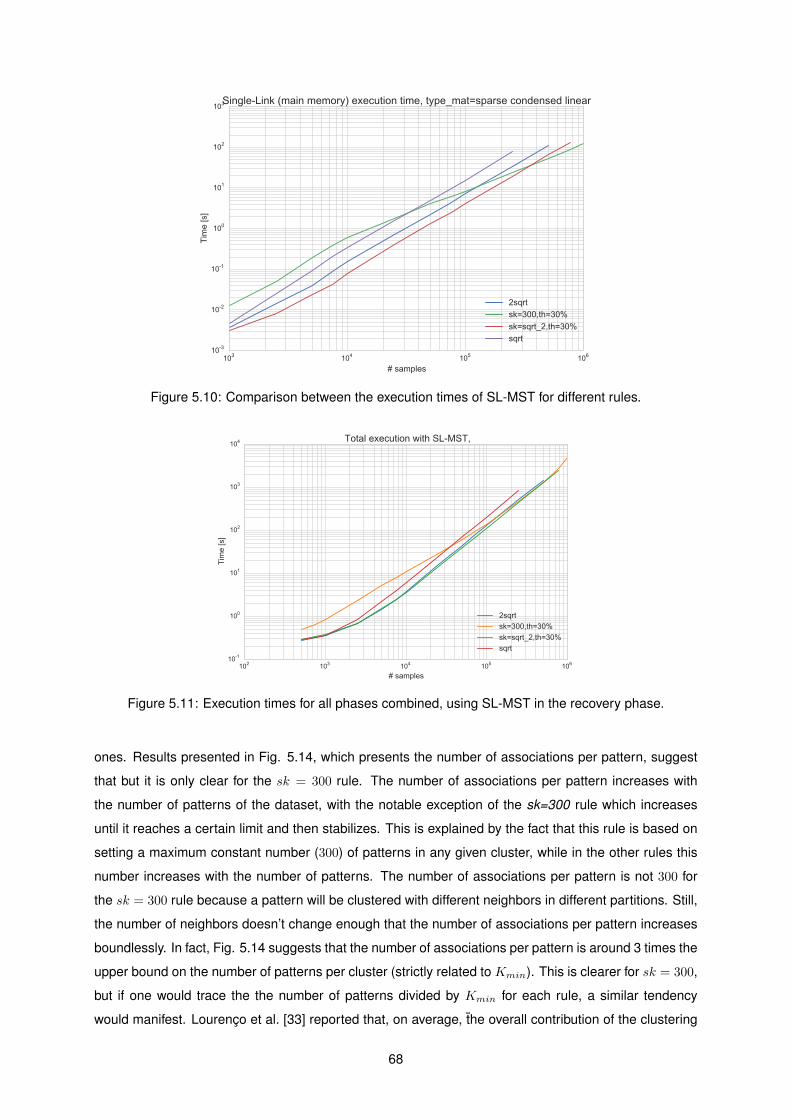
103 104 105 106
# samples
10-3
10-2
10-1
100
101
102
103
Tim
e [s
]
Single-Link (main memory) execution time, type_mat=sparse condensed linear
2sqrtsk=300,th=30%sk=sqrt_2,th=30%sqrt
Figure 5.10: Comparison between the execution times of SL-MST for different rules.
102 103 104 105 106
# samples
10-1
100
101
102
103
104
Tim
e [s
]
Total execution with SL-MST,
2sqrtsk=300,th=30%sk=sqrt_2,th=30%sqrt
Figure 5.11: Execution times for all phases combined, using SL-MST in the recovery phase.
ones. Results presented in Fig. 5.14, which presents the number of associations per pattern, suggest
that but it is only clear for the sk = 300 rule. The number of associations per pattern increases with
the number of patterns of the dataset, with the notable exception of the sk=300 rule which increases
until it reaches a certain limit and then stabilizes. This is explained by the fact that this rule is based on
setting a maximum constant number (300) of patterns in any given cluster, while in the other rules this
number increases with the number of patterns. The number of associations per pattern is not 300 for
the sk = 300 rule because a pattern will be clustered with different neighbors in different partitions. Still,
the number of neighbors doesn’t change enough that the number of associations per pattern increases
boundlessly. In fact, Fig. 5.14 suggests that the number of associations per pattern is around 3 times the
upper bound on the number of patterns per cluster (strictly related to Kmin). This is clearer for sk = 300,
but if one would trace the the number of patterns divided by Kmin for each rule, a similar tendency
would manifest. Lourenco et al. [33] reported that, on average, the overall contribution of the clustering
68

102 103 104 105 106 107
# samples
10-1
100
101
102
103
104
105
Tim
e [s
]
Total execution with SL-MST-Disk,
2sqrtsk=300,th=30%sk=sqrt_2,th=30%sqrt
Figure 5.12: Execution times for all phases combined, using SL-MST-Disk in the recovery phase.
ensemble (including unbalanced clusters) duplicates the co-associations produced in a single balanced
clustering with Kmin clusters. The spectrum of datasets evaluated regarding number of patterns was
smaller than that evaluated in the present work. The present results suggest a slightly higher value. So,
the decrease in density is more related with the quadratic growth of the full matrix in contrast with a
linear growth of the number of associations.
103 104 105 106 107
# samples
10-4
10-3
10-2
10-1
100
Den
sity
Density of associations relative to full matrix, type_mat=sparse condensed linear2sqrtsk=300,th=30%sk=sqrt_2,th=30%sqrt
Figure 5.13: Density of associations relative to the full co-association matrix, which hold n2 associations.
Predicting the number of associations before building the co-association matrix is useful for coming
up with combination schemes that are both memory and speed efficient. It was stated before that
the biggest cluster size in any partition of the ensemble is a good parameter for this end. Fig. 5.15
presents the relationship between the biggest cluster size and the maximum number of associations of
any pattern. These ratio increases with the number of patterns in the beginning, but as the number of
patterns increases it never goes over 3.
However, the number of features of the used datasets is rather reduced. It might be the case that this
69

103 104 105 106 107
# samples
101
102
103
104
No.
ass
ocia
tions
per
sam
ple
Number of associations per sample
Rule
2sqrtsk=300,th=30%sk=sqrt_2,th=30%sqrt
Figure 5.14: Evolution of the total number of associations divided by the number of patterns accordingto the different rules.
103 104 105 106 107
# samples
1.0
1.2
1.4
1.6
1.8
2.0
2.2
2.4
2.6
2.8
max
# a
ssoc
s / b
igge
st c
lust
er s
ize
Relationship between max. num. assocs and biggest cluster size per rule
2sqrtsk=300,th=30%sk=sqrt_2,th=30%sqrt
Figure 5.15: Maximum number of associations of any pattern divided by the number of patterns in thebiggest cluster of the ensemble.
ratio would increase with the number of features, since there would be more degrees where the clusters
might include other neighbors. With this in mind, further studies ranging a wider spectrum of datasets
should yield more enlightening conclusions or reinforce those presented here.
5.7.5 Space complexity
The previous section analyzed results related to the number of associations. This is related to the space
complexity of the different matrix formats, but does not present an accurate depiction of their complexity,
mainly due to the data structures supporting the sparse formats. The true space complexity of the
formats can be observed in Figures 5.16 and 5.17.
As explained previously, the allocated space for the space formats is based on a prediction that uses
the biggest cluster size of the ensemble. This allocated space is usually more than what is necessary
to store the total number of associations. Furthermore, the CSR sparse format, on which the EAC CSR
70

strategy is based, requires an array of the same size of the predicted number of associations. This
overhead may in fact make the sparse format pre-allocate more associations than actually are possible
for some rules, as can be seen in Fig. 5.16. Still, the allocated number of associations becomes a very
small fraction compared to the full matrix as the dataset complexity increases, which is typical case for
using a sparse format.
103 104 105 106 107
# samples
10-4
10-3
10-2
10-1
100
101
Den
sity
Density of allocated associations relative to full matrix, rule=sk=300,th=30%fullfull condensedsparse completesparse condensed constsparse condensed linear
Figure 5.16: Allocated number of associations relative to the full n2 matrix.
The actual memory used, presented in Fig. 5.17, follows roughly the same pattern. Here, the data
types used play a big role in the amount of memory that is required. Each association was stored in a
single byte, since the number of partitions was less than 255, as is usually the case. This means that the
memory used by the fully allocated formats is n2 and n(n−1)2 Bytes for the fully allocated complete and
condensed formats, respectively. In the sparse formats, the values of the associations were stored in an
array of unsigned integers of 1 Byte. However, an array of integers of 4 Bytes of the same size existed
to keep track of the destination pattern each association belongs to. Besides, one other array of integers
of 8 Bytes is kept but it is negligible compared to the other two arrays. The impact of the data types can
be seen for smaller datasets where the total memory used is actually significantly higher than that of the
full matrix. It should be noted that this discrepancy is not as high for other rules as for sk = 300. Still, the
sparse formats, and in particular the condensed sparse format, is preferred since the memory used for
large datasets is a small fraction of would be necessary if using any of the fully allocated formats. The
data types used depend on the problem at hand, since a user may choose to use a large ensemble or
have a very large
5.7.6 Accuracy
Finally, the accuracy of each solution was measured and is presented in Fig. 5.18. The number of
clusters of the final solutions was determined by the lifetime method. The accuracy was the same for
all rules and for all matrix formats in each dataset, except in the beginning were the sk = 300 produces
bad results due to the ensemble having partitions with a number of clusters inferior to the real number
71

103 104 105 106 107
# samples
10-3
10-2
10-1
100
101
102
Den
sity
Memory used relative to full matrix, rule=sqrtfullfull condensedsparse completesparse condensed constsparse condensed linear
Figure 5.17: Memory used relative to the full n2 matrix.
of clusters. Still, the sk = 300 rule is the one presented because it spans a wider spectrum of datasets.
When two classes are overlapping, the lifetime method typically interprets them as being the same class.
In the beginning, there are only two overlapping Gaussians, explaining the accuracy of roughly 84%. As
more patterns are added to the datasets, the accuracy lowers to around 66%, since now 4 classes are
overlapped in pairs. There are two lows in accuracy around the 50%. The first is due to a ”bridge”
between two classes by a couple of patterns that are not present in the surrounding datasets duo to
sampling. The last is duo to the same reason, since now more patterns are included in the dataset.
103 104 105 106 107
# samples
0.50
0.55
0.60
0.65
0.70
0.75
0.80
0.85
Mem
ory
ratio
Accuracy (CI) evolution with number of samplessk=300,th=30%
Figure 5.18: Accuracy of the final clusterings as measured with the Consistency Index.
5.8 Performance on real world datasets
The proposed EAC method was tested on real world datasets. Large real world datasets appropriate for
clustering were hard to find freely available. The datasets used are aimed at other Machine Learning
analysis, such as classification or regression. For this reason, the presented results are focused on
72

performance. Table 5.15 presents execution times for different phases of EAC on several real world
datasets. The ensemble size was of 30, the combination phase used sparse condensed matrices and
the sk=300 rule and the recovery phase was done with SL based on main memory. No comparison is
possible with the original implementation, since computation would not be possible. In most datasets
the production phase took the longest. The reason for this is that clusters in the ensemble were small
which led to fewer associations and, thus, more time spent in the production phase than in the others.
Furthermore, the recovery phase was fast because SL was based on main memory. Although high, the
computation times are acceptable for the processing of large datasets with a robust algorithm such as
EAC in a typical workstation.
Table 5.15: Execution times for real-world large datasets. P and F refer to the number of patterns andfeatures. P, C and R times refer to the production, combination and recovery times.
dataset alias # P # F P time [s] C time [s] R time [s]
PHYACT 1 [99] 441568 30 2158.69 123.85 19.76PHYACT 2 [99] 359170 30 1477.34 98.86 15.79esopH [100] 136127 2 17.94 35.15 3.95diabetes [101, 99] 101766 41 188.56 36.79 5.07
73

Chapter 6
Conclusions
6.1 Achievements
The main goal of this dissertation was scaling the EAC method for larger datasets than was previously
possible and speeding it up for smaller datasets. The EAC method is composed by three steps and, to
scale the whole method, each step was optimized separately while maintaining interoperability. During
this process, a dichotomy between optimizing for speed or memory usage appeared repeatedly. An
important lesson learn it that the right solution is not always obvious and one has to step back, ponder
how the optimizations in one part affect the whole and choose wisely.
The first step was the production of clustering ensembles, which was originally done with K-Means.
The space complexity was low compared to the whole algorithm, so the main focus was on speed opti-
mization. For that end, algorithms in the young field of quantum clustering were researched and tested.
Their computational complexity was shown to be prohibitive in the EAC context, which moved the re-
search to parallel computation, more specifically, GPGPU. A GPU parallel K-Means was implemented
and yielded positive results, effectively providing a speed-up over its sequential counterpart, ranging
from as low as 1.25 for high dimensional datasets to close to 25 for bidimensional datasets. On low
dimensional datasets the highest speed-up was observed with a high number of clusters, which is a
desirable result since EAC usually deals with a very high number of clusters in the ensemble’s parti-
tions. Still, the speed-ups observed are lower that those reported in literature for problems of similar
complexity. Since our results were produced from more modern machines, this shortcoming falls on the
implementation itself. The burdens of the API and language used, along with the absence of possible
optimizations, are the culprits for the sub-optimal performance.
In the combination step, the main problem for scaling was the space complexity. The clear solution
here was exploiting the sparse nature of the co-association matrix of EAC. After implementations of
sparse matrices in numerical libraries proved to be inadequate and literature lacked methods for effi-
ciently building a sparse matrix, the next direction was designing a strategy for efficiently building the
co-association matrix. This strategy, EAC CSR, was tested and shown to be much faster than other
sparse matrix implementations tested. Besides, it provided the much needed space complexity reduc-
74

tion that allowed the processing of large datasets.
For the recovery step, the SL algorithm was identified as the best candidate for optimization. This
was due to its relationship with MSTs, of which optimized implementations existed. GPU Boruvka was
reported to have significant speed-ups and was identified has the best parallel GPU MST algorithm in
literature. It was implemented but it showed to not be able to handle the lower sparsity of EAC co-
associations graphs. This moved the focus of optimization of this step to external memory algorithms,
which, although slower, were what ultimately allowed for the final processing of EAC in large datasets.
The main contributions to the EAC method, by step, were the GPU parallel K-Means in the produc-
tion step, the EAC CSR strategy in the combination step and the SL-MST-Disk in the recovery step. New
Kmin rules for optimizing the sparsity of the co-association matrix were proposed and a deeper under-
standing of how they affect the properties of EAC are also relevant contributions. These contributions
together allow for the application of the EAC method to datasets whose complexity was not handled
by the original implementation. Furthermore, the proposed optimized version is also faster for smaller
datasets.
6.2 Future Work
Naturally, during the research and development of the present work, divergent lines of research were
deemed interesting. Occasionally, shortcomings in the present work were identified for which possible
solutions were envisioned. Time restrictions have moved those possible solutions and lines of research
from the main body of the present work to this section of recommendations for future work.
An obvious line of work is porting the work here presented to other technologies. As an example,
the GPU algorithms could be implemented in OpenCL. This would bring major benefits in respect to
portability since OpenCL supports most devices. Moreover, OpenCL’s performance is becoming closer
to CUDA’s and since it’s programming model was based on CUDA, it should be straightforward for a
developers to make the switch.
The implementation of the GPU K-Means could be improved by using shared memory. Each block
of threads would read centroids to this memory which would decrease the number of fetches to global
memory significantly and therefore improve performance. A study of the optimal block size and a more
thorough study of the optimal number of patterns to process in each thread are also relevant lines of
research.
Dynamic Parallelism offers the ability of having a kernel call on other kernel without intervention from
the host. This translates in the possibility of moving the control logic in the Boruvka variant to the device,
effectively removing the memory transfer of values related with the control logic.
A possible way to further reducing the space complexity of the recovery step is threshold cut-off of
associations, i.e. cutting associations in the co-association matrix that are weaker than a certain thresh-
old. The underlying idea is that strong associations will have the bigger effect on the final clustering,
while the weak will have little to no effect. This assumption could allow for the reduction of space com-
plexity while keeping the final accuracy, or even improving it by cutting bad associations. This line of
75

research was briefly explored on small datasets and is in fact implemented, but robust testing was not
possible. The main challenge here is to find safe thresholds that will not damage the overall quality of
the results.
A good follow-up of the present work is to study the relationship between several metrics (e.g. spar-
sity, accuracy, maximum number of co-associations) and the complexity of the dataset. Several mea-
sures for describing the complexity of the dataset exist [102] and it would be interesting to profile several
datasets of different complexities and structures and analyze the relationship between these complexity
measures and EAC properties. On a performance perspective it could prove useful to deduce better
rules to set the maximum number of associations in the sparse matrix. On a accuracy perspective it
would be interesting to see if there are types of datasets that simply are not a good fit for EAC while
other are, as well as perform automatic choosing of the Kmin parameter. It would also be interesting to
relate complexity with the threshold cut-off.
The WEAC algorithm, presented in chapter 2, is focused on improving accuracy. The underlying
concept is to measure the quality of the partitions in the ensemble and allow the better ones to be more
influential in the co-association matrix. The concept of measuring the quality of the partitions may prove
useful for further decreasing the memory complexity with the EAC CSR scheme without compromising
accuracy. The basic idea is to choose a max assocs value that will likely be less than the number
of associations many patterns will have, which will result in some associations being discarded. The
associations that will be kept are the ones from the first partitions that were processed. With this in
mind, one could order the partitions by quality and start the processing from those with better quality.
This would increase the likelihood that the discarded associations are, in fact, weaker associations.
A possible extension to EAC CSR is allowing for bigger than main memory co-association matrices.
An approach for this would be to divide the co-association matrix in several parts. The entire ensemble
would then have to be processed for each of these parts, but it would allow for the processing of even
larger datasets than is now possible.
Two ways of dealing with the space complexity of EAC were identified in literature: exploiting sparsity
and using k-Nearest Neighbors. Building a k-Nearest Neighbors co-association matrix requires two
matrices: one for holding the association values and another for holding the neighbors of each pattern.
The mechanism for building this co-association matrix was implemented but it was not possible to make
it inter-operable with the final step of EAC. However, this should be a straightforward process since its
conversion to EAC CSR is can be done simply by linearizing both matrices. The values matrix would
become the data array, the neighbors matrix would be the indices array and finally an indptr array would
have to be created, which is straighforward, since the number of neighbors of each pattern is constant.
The argsort operation in the recovery step is one of the most computationally intensive. This opera-
tion is typically done by sorting chunks of the array in main memory and then merging them. The external
algorithm used for this operation has a very low main memory profile. However, when it is executed most
main memory is free. This means that a more efficient algorithm for performing this operation is possible
simply by using more main memory, and therefore processing bigger chunks at a time. Besides, it is
believed that a significant speed-up may be obtained by using GPUs for sorting these chunks.
76

Much effort was put into developing and testing co-association matrix building strategies. The
schemes presented here provide a solid framework to work with large datasets in the middle step of
EAC. As such, interesting directions for this work to take include researching and testing how state of
the art algorithms designed for Big Data would complement EAC in the first and last steps.
77

78

References
[1] Diogo Silva, Ana Fred, and Helena Aidos. Efficient Evidence Accumulation Clustering for Large
Datasets. Proccedings of the 5th International Conference on Pattern Recognition Applications
and Methods, (Accepted), 2016.
[2] Anil K Jain. Data clustering: 50 years beyond K-means. Pattern Recognition Letters, 31(8):
651–666, 2010.
[3] a. K. Jain, M. N. Murty, and P. J. Flynn. Data clustering: a review. ACM Computing Surveys, 31
(3):264–323, 1999.
[4] Edgar Anderson. The species problem in Iris. Annals of the Missouri Botanical Garden, pages
457–509, 1936.
[5] Ronald A Fisher. The use of multiple measurements in taxonomic problems. Annals of eugenics,
7(2):179–188, 1936.
[6] Raymond A Jarvis and Edward A Patrick. Clustering using a similarity measure based on shared
near neighbors. Computers, IEEE Transactions on, 100(11):1025–1034, 1973.
[7] Charu C Aggarwal and Chandan K Reddy. Data clustering: algorithms and applications. CRC
Press, 2013.
[8] Ana Fred. Finding consistent clusters in data partitions. Multiple classifier systems, pages 309–
318, 2001.
[9] Marina Meila. Comparing clusterings by the variation of information. Learning theory and Kernel
machines: 16th Annual Conference on Learning Theory and 7th Kernel Workshop, COLT/Kernel
2003, Washington, DC, USA, August 24-27, 2003: proceedings, page 173, 2003.
[10] David L Davies and Donald W Bouldin. A cluster separation measure. Pattern Analysis and
Machine Intelligence, IEEE Transactions on, (2):224–227, 1979.
[11] Daniel Boley. Principal Direction Divisive Partitioning. Data Mining and Knowledge Discovery, 2
(4):325–344, 1998.
[12] Michael Steinbach, George Karypis, Vipin Kumar, and Others. A comparison of document clus-
tering techniques. KDD workshop on text mining, 400(1):525–526, 2000.
79

[13] Marie Chavent. A monothetic clustering method. Pattern Recognition Letters, 19(11):989–996,
1998.
[14] James C. Bezdek, Robert Ehrlich, and William Full. FCM: The Fuzzy C-Means Clustering Algo-
rithm. Computers & Geosciences, 10(2–3):191–203, 1984.
[15] U Kang, Charalampos E Tsourakakis, and Christos Faloutsos. PEGASUS : Mining Peta-Scale
Graphs. Knowledge and Information Systems, 27(2):303–325, 2011.
[16] J B MacQueen. Some Methods for classification and Analysis of Multivariate Observations. In
Proceedings of 5-th Berkeley Symposium on Mathematical Statistics and Probability, Berkeley,
University of California Press, volume 1, pages 281–297, 1967.
[17] D. Arthur, D. Arthur, S. Vassilvitskii, and S. Vassilvitskii. k-means++: The advantages of careful
seeding. Proceedings of the eighteenth annual ACM-SIAM symposium on Discrete algorithms, 8:
1027–1035, 2007.
[18] Malay K Pakhira. A Modified k -means Algorithm to Avoid Empty Clusters. International Journal
of Recent Trends in Enineering, 1(1), 2009.
[19] Peter H A Sneath and Robert R Sokal. Numerical taxonomy. Nature, 193(4818):855–860, 1962.
[20] R. Sibson. SLINK: an optimally efficient algorithm for the single-link cluster method. The Computer
Journal, 16(1):30–34, 1973.
[21] J. C. Gower and G. J. S. Ross. Minimum Spanning Trees and Single Linkage Cluster Analysis.
Journal of the Royal Statistical Society, 18(1):54–64, 1969.
[22] Daniel Mullner. Modern hierarchical, agglomerative clustering algorithms. arXiv preprint
arXiv:1109.2378, 2011.
[23] J-L Starck and Fionn Murtagh. Astronomical image and data analysis. Springer Science & Busi-
ness Media, 2007.
[24] Alexander Topchy, Anil K Jain, and William Punch. A mixture model for clustering ensembles. In
Society for Industrial and Applied Mathematics. Proceedings of the SIAM International Conference
on Data Mining, page 379. Society for Industrial and Applied Mathematics, 2004.
[25] Ana N L Fred and Anil K Jain. Combining multiple clusterings using evidence accumulation. IEEE
Transactions on Pattern Analysis and Machine Intelligence, 27(6):835–850, 2005.
[26] Alexander Strehl and Joydeep Ghosh. Cluster Ensembles – A Knowledge Reuse Framework for
Combining Multiple Partitions. Journal of Machine Learning Research, 3:583–617, 2002.
[27] Hongjun Wang, Hanhuai Shan, and Arindam Banerjee. Bayesian cluster ensembles. Statistical
Analysis and Data Mining: The ASA Data Science Journal, 4(1):54–70, 2011.
80

[28] Sandrine Dudoit and Jane Fridlyand. Bagging to improve the accuracy of a clustering procedure.
Bioinformatics, 19(9):1090–1099, 2003.
[29] Ana N L Fred and Anil K Jain. Data clustering using evidence accumulation. In Pattern Recogni-
tion, 2002. Proceedings. 16th International Conference on, volume 4, pages 276–280, 2002.
[30] Andre Lourenco and Ana Fred. Ensemble methods in the clustering of string patterns. Proceed-
ings - Seventh IEEE Workshop on Applications of Computer Vision, WACV 2005, pages 143–148,
2007.
[31] Andre Lourenco, Carlos Carreiras, Samuel Rota Bulo, and Ana Fred. ECG analysis using con-
sensus clustering. In Signal Processing Conference (EUSIPCO), 2014 Proceedings of the 22nd
European, pages 511–515. IEEE, 2014.
[32] F.J. Duarte, a.L.N. Fred, a. Lourenco, and M.F. Rodrigues. Weighting Cluster Ensembles in Evi-
dence Accumulation Clustering. 2005 Portuguese Conference on Artificial Intelligence, 00:159–
167, 2005.
[33] Andre Lourenco, Ana L N Fred, and Anil K. Jain. On the scalability of evidence accumulation
clustering. Proceedings - International Conference on Pattern Recognition, 0:782–785, 2010.
[34] You Wen Qian, William Cukierski, Mona Osman, and Lauri Goodell. Combined multiple clusterings
on flow cytometry data to automatically identify chronic lymphocytic leukemia. ICBBT 2010 - 2010
International Conference on Bioinformatics and Biomedical Technology, pages 305–309, 2010.
[35] L O’Callaghan, N Mishra, A Meyerson, S Guha, and R Motwani. Streaming-data algorithms for
high-quality clustering. In Data Engineering, 2002. Proceedings. 18th International Conference
on, pages 685–694, 2002.
[36] Raymond T Ng and Jiawei Han. Clarans: A method for clustering objects for spatial data mining.
Knowledge and Data Engineering, IEEE Transactions on, 14(5):1003–1016, 2002.
[37] Tian Zhang, Raghu Ramakrishnan, and Miron Livny. BIRCH: an efficient data clustering method
for very large databases. In ACM SIGMOD Record, volume 25, pages 103–114. ACM, 1996.
[38] Sudipto Guha, Rajeev Rastogi, and Kyuseok Shim. CURE: an efficient clustering algorithm for
large databases. In ACM SIGMOD Record, volume 27, pages 73–84. ACM, 1998.
[39] Petros Drineas, Ravi Kannan, and Michael W Mahoney. Fast Monte Carlo algorithms for matrices
III: Computing a compressed approximate matrix decomposition. SIAM Journal on Computing, 36
(1):184–206, 2006.
[40] Mario Zechner and Michael Granitzer. K-Means on the Graphics Processor: Design And Experi-
mental Analysis. International Journal on Advances in System and Measurements, 2(2):224–235,
2009.
81

[41] Wen-Yen Chen, Yangqiu Song, Hongjie Bai, Chih-Jen Lin, and Edward Y Chang. Parallel spectral
clustering in distributed systems. Pattern Analysis and Machine Intelligence, IEEE Transactions
on, 33(3):568–586, 2011.
[42] Hong Tao Bai, Li Li He, Dan Tong Ouyang, Zhan Shan Li, and He Li. K-means on commodity GPUs
with CUDA. 2009 WRI World Congress on Computer Science and Information Engineering, CSIE
2009, 3:651–655, 2009.
[43] Jiadong Wu and Bo Hong. An efficient k-means algorithm on CUDA. IEEE International Sym-
posium on Parallel and Distributed Processing Workshops and Phd Forum, pages 1740–1749,
2011.
[44] Mario Zechner and Michael Granitzer. Accelerating k-means on the graphics processor via CUDA.
Proceedings of the 1st International Conference on Intensive Applications and Services, INTEN-
SIVE 2009, pages 7–15, 2009.
[45] J Sirotkovi, H Dujmi, and V Papi. K-means image segmentation on massively parallel GPU ar-
chitecture. In MIPRO, 2012 Proceedings of the 35th International Convention, pages 489–494,
2012.
[46] Reza Farivar, Daniel Rebolledo, and Ellick Chan. A parallel implementation of k-means clustering
on GPUs. In The 2008 International Conference on Parallel and Distributed Processing Tech-
niques and Applications, pages 340–345, 2008.
[47] Jeffrey DiMarco and Michela Taufer. Performance impact of dynamic parallelism on different clus-
tering algorithms. In Proc. SPIE 8752, Modeling and Simulation for Defense Systems and Appli-
cations VIII, pages 87520E—-87520E, 2013.
[48] Vibhav Vineet, Pawan Harish, Suryakant Patidar, and P J Narayanan. Fast minimum spanning tree
for large graphs on the GPU. In Proceedings of the Conference on High Performance Graphics
2009, pages 167–171. ACM, 2009.
[49] Scott Rostrup, Shweta Srivastava, and Kishore Singhal. Fast and memory-efficient minimum
spanning tree on the GPU. International Journal of Computational Science and Engineering, 8(1):
21–33, 2013.
[50] C Da Silva Sousa, A Mariano, and A Proenca. A Generic and Highly Efficient Parallel Variant of
Boruvka’s Algorithm. In Parallel, Distributed and Network-Based Processing (PDP), 2015 23rd
Euromicro International Conference on, pages 610–617, 2015.
[51] Joseph B Kruskal. On the shortest spanning subtree of a graph and the traveling salesman
problem. Proceedings of the American Mathematical society, 7(1):48–50, 1956.
[52] Robert Clay Prim. Shortest connection networks and some generalizations. Bell system technical
journal, 36(6):1389–1401, 1957.
82

[53] Otakar Boruvka. O jistem problemu minimalnım. Prace Moravske Prirodovedecke Spolecnosti, 3:
37–58, 1926.
[54] Wei Wang, Yongzhong Huang, and Shaozhong Guo. Design and Implementation of GPU-Based
Prim ’ s Algorithm. International Journal of Modern Education and Computer Science, 4(July):
55–62, 2011.
[55] Pawan Harish, Vibhav Vineet, and P J Narayanan. Large graph algorithms for massively multi-
threaded architectures. International Institute of Information Technology Hyderabad, Tech. Rep.
IIIT/TR/2009/74, 2009.
[56] W. Daniel Hillis and Guy L. Steele. Data parallel algorithms. Communications of the ACM, 29(12):
1170–1183, 1986.
[57] Guy E Blelloch. Prefix Sums and Their Applications, chapter 1, pages 35–60. 1993.
[58] Mark Harris, Shubhabrata Sengupta, and John D. Owens. Parallel Prefix Sum (Scan) with CUDA
Mark. Gpu gems 3, (April):1–24, 2007.
[59] Esma Aımeur, Gilles Brassard, and Sebastien Gambs. Quantum speed-up for unsupervised learn-
ing. Machine Learning, 90(February 2012):261–287, 2013.
[60] Seth Lloyd, Masoud Mohseni, and Patrick Rebentrost. Quantum algorithms for supervised and
unsupervised machine learning. arXiv preprint arXiv:1307.0411, 2013.
[61] Lov K Grover. A fast quantum mechanical algorithm for database search. In Proceedings of the
twenty-eighth annual ACM symposium on Theory of computing, pages 212–219. ACM, 1996.
[62] Nathan Wiebe, Ashish Kapoor, and Krysta Svore. Quantum Algorithms for Nearest-Neighbor
Methods for Supervised and Unsupervised Learning. arXiv preprint arXiv:1401.2142, page 31,
2014.
[63] Richard P. Feynman. Simulating physics with computers. International Journal of Theoretical
Physics, 21(6-7):467–488, 1982.
[64] Peter Wittek. Quantum Machine Learning: What Quantum Computing Means to Data Mining.
Academic Press, 2014.
[65] Ellis Casper and Chih-cheng Hung. Quantum Modeled Clustering Algorithms for Image Segmen-
tation. Progress in Intelligent Computing and Applications, 2:1–21, 2013.
[66] Kuk-Hyun Han and Jong-Hwan Kim. Genetic quantum algorithm and its application to combi-
natorial optimization problem. Proceedings of the 2000 Congress on Evolutionary Computation.
CEC00 (Cat. No.00TH8512), 2, 2000.
[67] Wenjie Liu, Hanwu Chen, Qiaoqiao Yan, Zhihao Liu, Juan Xu, and Yu Zheng. A novel quantum-
inspired evolutionary algorithm based on variable angle-distance rotation. 2010 IEEE World
83

Congress on Computational Intelligence, WCCI 2010 - 2010 IEEE Congress on Evolutionary
Computation, CEC 2010, 2010.
[68] H Talbi, A Draa, and M Batouche. A new quantum-inspired genetic algorithm for solving the trav-
elling salesman problem. In Industrial Technology, 2004. IEEE ICIT ’04. 2004 IEEE International
Conference on, volume 3, pages 1192–1197, 2004.
[69] Ellis Casper, Chih-Cheng Hung, Edward Jung, and Ming Yang. A Quantum-Modeled K-Means
Clustering Algorithm for Multi-band Image Segmentation. In Proceedings of the 2012 ACM Re-
search in Applied Computation Symposium, volume 1, pages 158–163, 2012.
[70] Jing Xiao, YuPing Yan, Jun Zhang, and Yong Tang. A quantum-inspired genetic algorithm for
k-means clustering. Expert Systems with Applications, 37:4966–4973, 2010.
[71] Chih-Cheng Hung, Ellis Casper, Bor-chen Kuo, Wenping Liu, Edward Jung, Ming Yang, Xiaoyi Yu,
Edward Jung, and Ming Yang. A Quantum-Modeled Artificial Bee Colony clustering algorithm for
remotely sensed multi-band image segmentation. In Geoscience and Remote Sensing Sympo-
sium (IGARSS), 2013 IEEE International, pages 2501–2504. IEEE, 2013.
[72] Chih-Cheng Hung, Ellis Casper, Bor-Chen Kuo, Wenping Liu, Xiaoyi Yu, Edward Jung, and Ming
Yang. A Quantum-Modeled Fuzzy C-Means clustering algorithm for remotely sensed multi-band
image segmentation. In Geoscience and Remote Sensing Symposium (IGARSS), 2013 IEEE
International, pages 2501–2504. IEEE, 2013.
[73] Shenshen Liang, Cheng Wang, Ying Liu, and Liheng Jian. CUKNN: A parallel implementation
of K-nearest neighbor on CUDA-enabled GPU. Proceedings - 2009 IEEE Youth Conference on
Information, Computing and Telecommunication, YC-ICT2009, pages 415–418, 2009.
[74] Yangyang Li, Nana Wu, Jingjing Ma, and Licheng Jiao. Quantum-inspired immune clonal cluster-
ing algorithm based on watershed. In IEEE Congress on Evolutionary Computation, pages 1–7.
IEEE, jul 2010.
[75] Said M Mikki, Ahmed Kishk, and Others. Quantum particle swarm optimization for electromagnet-
ics. Antennas and Propagation, IEEE Transactions on, 54(10):2764–2775, 2006.
[76] David Horn and Assaf Gottlieb. Algorithm for Data Clustering in Pattern Recognition Problems
Based on Quantum Mechanics. Physical Review Letters, 88(1):1–4, 2001.
[77] Marvin Weinstein and David Horn. Dynamic quantum clustering: a method for visual exploration
of structures in data. Physical Review E - Statistical, Nonlinear, and Soft Matter Physics, 80(6):
1–15, 2009.
[78] Zhi-Hua Li, Shi-Tong Wang, and Jiangsu Wuxi. Quantum Theory: The unified framework for FCM
and QC algorithm. In Wavelet Analysis and Pattern Recognition, 2007. ICWAPR’07. International
Conference on, volume 3, pages 1045–1048. IEEE, 2007.
84

[79] Hao Wang, Shiqin Yang, Wenbo Xu, and Jun Sun. Scalability of Hybrid Fuzzy C-Means Algorithm
Based on Quantum-Behaved PSO. In Fourth International Conference on Fuzzy Systems and
Knowledge Discovery (FSKD 2007), volume 2, pages 261–265, 2007.
[80] Jun Sun, Bin Feng, and Wenbo Xu. Particle swarm optimization with particles having quantum
behavior. In Evolutionary Computation, 2004. CEC2004. Congress on, volume 1, pages 325–331
Vol.1, 2004.
[81] a. Manju and M. J. Nigam. Applications of quantum inspired computational intelligence: A survey.
Artificial Intelligence Review, 42:79–156, 2014.
[82] Marco Lanzagorta and Jeffrey Uhlmann. Quantum Computer Science, volume 1. 2008.
[83] David Rosenbaum and Aram W. Harrow. Uselessness for an Oracle Model with Internal Random-
ness. arXiv:1111.1462, pages 1–23, 2011.
[84] David Horn, Tel Aviv, Assaf Gottlieb, Hod HaSharon, Inon Axel, and Ramat Gan. Method and
Apparatus for Quantum Clustring, 2010.
[85] David Horn and Assaf Gottlieb. The Method of Quantum Clustering. In NIPS, pages 769—-776,
2001.
[86] Peter Wittek. High-performance dynamic quantum clustering on graphics processors. Journal of
Computational Physics, 233:262–271, 2013.
[87] Stefan Van Der Walt, S. Chris Colbert, and Gael Varoquaux. The NumPy array: A structure for
efficient numerical computation. Computing in Science and Engineering, 13(2):22–30, 2011.
[88] Eric Jones, Travis Oliphant, Pearu Peterson, and Others. SciPy: Open source scientific tools for
Python. URL http://www.scipy.org/.
[89] Travis E. Oliphant. Python for scientific computing. Computing in Science and Engineering, 9(3):
10–20, 2007.
[90] K. Jarrod Millman and Michael Aivazis. Python for scientists and engineers. Computing in Science
and Engineering, 13(2):9–12, 2011.
[91] John D Hunter. Matplotlib: A 2D graphics environment. Computing in science and engineering, 9
(3):90–95, 2007.
[92] Wes McKinney. Data Structures for Statistical Computing in Python. Proceedings of the 9th
Python in Science Conference, 1697900(Scipy):51–56, 2010.
[93] Fabian Pedregosa, Gael Varoquaux, Alexandre Gramfort, Vincent Michel, Bertrand Thirion, Olivier
Grisel, Mathieu Blondel, Peter Prettenhofer, Ron Weiss, Vincent Dubourg, Jake Vanderplas,
Alexandre Passos, David Cournapeau, Matthieu Brucher, Matthieu Perrot, and Edouard Duch-
esnay. Scikit-learn: Machine Learning in Python. Journal of Machine Learning Research, 12
(Oct):2825–2830, 2011.
85

[94] Fernando Perez and Brian E. Granger. IPython: A system for interactive scientific computing.
Computing in Science and Engineering, 9(3):21–29, 2007.
[95] Numba Development Team. Numba, 2015. URL http://numba.pydata.org.
[96] Francesc Alted, Ivan Vilata, and Others. PyTables: Hierarchical Datasets in Python. URL http:
//www.pytables.org/.
[97] The HDF Group. Hierarchical Data Format, version 5.
[98] Francesc Altet i Abad and Ivan Vilata Balaguer. OPSI : The indexing system of PyTables 2 Pro-
fessional Edition. Technical report, 2007. URL http://www.pytables.org/docs/OPSI-indexes.
pdf.
[99] M Lichman. {UCI} Machine Learning Repository, 2013. URL http://archive.ics.uci.edu/ml.
[100] E S Yuksel, J C Slaughter, N Mukhtar, M Ochieng, G Sun, M Goutte, S Muddana, C Gaelyn
Garrett, and M F Vaezi. An oropharyngeal pH monitoring device to evaluate patients with chronic
laryngitis. Neurogastroenterology and motility : the official journal of the European Gastrointestinal
Motility Society, 25(5), 2013.
[101] Beata Strack, Jonathan P DeShazo, Chris Gennings, Juan L Olmo, Sebastian Ventura, Krzysztof J
Cios, and John N Clore. Impact of HbA1c measurement on hospital readmission rates: analysis
of 70,000 clinical database patient records. BioMed research international, 2014, 2014.
[102] Tin K Ho and Mitra Basu. Complexity measures of supervised classification problems. IEEE
Transactions on Pattern Analysis and Machine Learning, 24(3):289–300, 2002.
[103] Linchuan Chen and Gagan Agrawal. Optimizing MapReduce for GPUs with Effective Shared
Memory Usage. Proceedings of the 21st international symposium on High-Performance Parallel
and Distributed Computing (HPDC’12), pages 199–210, 2012.
[104] Ren Wu, Bin Zhang, and Meichun Hsu. Clustering billions of data points using GPUs. Proceed-
ings of the combined workshops on UnConventional high performance computing workshop plus
memory access workshop, pages 1–5, 2009.
[105] S Shalom, Manoranjan Dash, Minh Tue, and Nithin Wilson. Hierarchical Agglomerative Cluster-
ing Using Graphics Processor with Compute Unified Device Architecture. In 2009 International
Conference on Signal Processing Systems, ICSPS 2009, pages 556–561, 2009.
[106] S Shalom and Manoranjan Dash. Efficient hierarchical agglomerative clustering algorithms on
GPU using data partitioning. In Parallel and Distributed Computing, Applications and Technologies
(PDCAT), 2011 12th International Conference on, pages 134–139, 2011.
[107] Yanjun Jiang, Enxing Li, and Zhanchun Gao. A GPU-based harmony k-means algorithm for doc-
ument clustering. In Information Science and Control Engineering 2012 (ICISCE 2012), IET Inter-
national Conference on, pages 1–4, 2012.
86

[108] Ranajoy Malakar and Naga Vydyanathan. A CUDA-enabled hadoop cluster for fast distributed im-
age processing. 2013 National Conference on Parallel Computing Technologies, PARCOMPTECH
2013, 2013.
[109] Max Grossman, Mauricio Breternitz, and Vivek Sarkar. HadoopCL: MapReduce on distributed
heterogeneous platforms through seamless integration of hadoop and OpenCL. Proceedings
- IEEE 27th International Parallel and Distributed Processing Symposium Workshops and PhD
Forum, IPDPSW 2013, pages 1918–1927, 2013.
[110] Marko J Misi, M C, and Milo V Tomasevi. Evolution and Trends in GPU Computing. MIPRO, 2012
Proceedings of the 35th International Convention, pages 289–294, 2012.
[111] Feng Ji and Xiaosong Ma. Using Shared Memory to Accelerate MapReduce on Graphics Process-
ing Units. 2011 IEEE International Parallel & Distributed Processing Symposium, pages 805–816,
2011.
[112] Miao Xin and Hao Li. An implementation of GPU accelerated MapReduce: Using Hadoop with
OpenCL for data- and compute-intensive jobs. In Proceedings - 2012 International Joint Con-
ference on Service Sciences, Service Innovation in Emerging Economy: Cross-Disciplinary and
Cross-Cultural Perspective, IJCSS 2012, pages 6–11, 2012.
[113] Bingsheng He, Weibin Fang, Qiong Luo, Naga K Govindaraju, and Tuyong Wang. Mars: a MapRe-
duce framework on graphics processors. In Proceedings of the 17th international conference on
Parallel architectures and compilation techniques, pages 260–269, 2008.
[114] Kamran Karimi, Neil G. Dickson, and Firas Hamze. A Performance Comparison of CUDA and
OpenCL. arXiv preprint arXiv:1005.2581, 2010.
[115] Ching Lung Su, Po Yu Chen, Chun Chieh Lan, Long Sheng Huang, and Kuo Hsuan Wu. Overview
and comparison of OpenCL and CUDA technology for GPGPU. IEEE Asia-Pacific Conference on
Circuits and Systems, Proceedings, APCCAS, pages 448–451, 2012.
[116] Nvidia. CUDA C Programming Guide. Programming Guides, (August), 2015.
87

88

Appendix A
General Purpose computing on
Graphical Processing Units
The original intended use for GPUs was graphics processing, hence its name. Recently, GPUs have
been increasingly used for other purposes - a trend commonly known as General Purpose process-
ing in Graphics Processing Units (GPGPU). GPU present a solution for ”extreme-scale, cost-effective,
and power-efficient high performance computing” [103]. Furthermore, GPUs are common in consumer
desktops and laptops, effectively bringing this computation power to the masses.
GPUs were typically useful for users that required high performance graphics computation. Other ap-
plications were soon explored as users from different fields realized the high parallel computation power
of these devices. However, the architecture of the GPUs themselves has been strictly oriented toward
the graphics computing until the appearance of specialized GPU models designed for data computation
(e.g. NVIDIA Tesla).
GPGPU application on several fields and algorithms has been reported with significant performance
increase, e.g. application on the K-Means algorithm [42, 43, 44, 104], hierarchical clustering [105, 106],
document clustering [107], image segmentation [45], integration in Hadoop clusters [108, 109], among
other applications.
Current GPUs pack hundreds of cores and have a better energy/area ratio than traditional infrastruc-
ture. GPU work under the SIMD framework, i.e. all the cores in the device execute the same code at the
same time and only the data changes over time.
A.1 Programming GPUs
In the very beginning of GPGPU, programming was done directly through graphics APIs. Program-
ming for GPUs was traditionally done within the paradigm of graphics processing, such as DirectX and
OpenGL. If researchers and programmers wanted to tap into the computing power of a GPU they had to
learn and use these APIs and frameworks, which is a challenging task since their general problems had
to be modelled to the graphics-oriented primitives [110]. With the appearance of DirectX 9, shader pro-
89
gramming languages of higher level became available (e.g. C for graphics, DirectX High Level Shader
Language, OpenGL Shading Language), but they were still inherently graphics programming languages,
where computation must be expressed in graphics terms.
More recent programming models, such as CUDA and OpenCL, removed a lot of that burden by ex-
posing the power of GPUs in a way closer to traditional programming. Currently, the major programming
models used for computation in GPU are OpenCL and CUDA. While the first is widely available in most
devices, the latter is only available for NVIDIA devices.
As Google’s MapReduce computing model has increasingly become a standard for scalable and
distributed computing over big data, attempts have been made to port the model to the GPU [111, 112,
113]. This translates in using the same programming model over a wide array of computing platforms.
A.2 OpenCL vs CUDA
Presently, the most mature programming models are CUDA and OpenCL. CUDA appeared first and
is supported only by NVidia devices. It is also the most mature of the two and performs well since it
was designed alongside with the hardware architecture of the supporting devices. OpenCL has the
advantage of portability, but that comes with issues of performance portability. Both models are, in fact,
very similar and literature suggests that porting the code from one to the other requires minimal changes
[114, 115]. Literature also reports that CUDA performs better than OpenCL [115] for equivalent code.
A.3 Overview of CUDA
This section presents an overview of the CUDA programming model and its main concepts and charac-
teristics. For a more thorough and extensive explanation of this topic, the CUDA C Programming Guides
[116], the source of the present review, should be consulted. A GPU is comprised by one or several
streaming processors (or multiprocessor). Each of these processors contains several simpler proces-
sors, each of which execute the same instruction at the same time at any given time. In the CUDA
programming model, the basic unit of computation is a thread. Threads are grouped into blocks which
are part of the block grid. The number of threads in a block is typically higher than the number of proces-
sors in a multiprocessor. For that reason, the hardware automatically divides the threads from a block
into smaller batches, called warps. This hierarchy is represented in Figure A.1. The computation of one
block is independent from other blocks and each block is scheduled to one multiprocessor, which means
that more multiprocessors results in more blocks being processed at the same time, as represented in
Figure A.2.
Block configuration can be multidimensional, up to and including 3 dimensions. Furthermore, there
is a limit in the amount of threads in each dimension that varies with the GPU being used, e.g. for GPUs
with CUDA compute capability 2.x the maximum number of threads is 1024 for the x- or y-dimensions,
64 for the z-dimension, an overall maximum number of threads of 1024 and a warp size of 32 threads.
90

Figure A.1: Thread hierarchy [116].
Figure A.2: Distribution of thread blocks isautomatically scaled with the increase of thenumber of multiprocessors [116].
Instructions are issued per warp and registers and shared memory are allocated for an active block.
A block will remain active until all threads have finished. When operands are not ready the warp is
stalled and the context switches to another warp. Streaming processors have a limit to the maximum
number of active warps, depending on the GPU. Choosing a block size is not trivial, as it is necessary to
understand the characteristics of the kernel and the used GPU. The ratio between the number of active
warps per multiprocessor and the maximum number of warps that can be active is called occupancy
and a high occupancy is often used as a way to choose a good block size. The idea is to hide latency
during global memory loads followed by thread synchronizations by maximizing the number of active
warps, i.e. maximizing occupancy. Occupancy limiters include registers per thread, shared memory per
block and threads per block. NVIDIA supplies a CUDA Occupancy Calculator to aid the programmer in
tweaking block size, considering the other limiters.
Depending on the architecture, GPUs have several types of memories. Accessible to all cores (and
threads) are the global memory, constant memory and texture memory, of which the last two are read-
only. Blocks share a smaller but significantly faster memory called shared memory, which is a memory
inside a multiprocessor to which all cores have access to, enabling inter-thread communication inside
a block. Finally, each thread has access to local memory. Local memory resides in global memory
space and has the same latency for read and write operations. However, if the thread is using only
single variables or constant sized arrays, it uses register space, which is very fast. If the memory used
exceeds the available register space the local memory used. This memory hierarchy is represented in
Figure A.3.
The typical flow of a CUDA application (and, typically, any modern GPU application) is explained in
this paragraph and can be observed in Figure A.4. First, the host CPU is responsible for several steps
in the set-up phase. The host starts by transferring any necessary data to the device memory (global,
91

Figure A.3: Memory model used by CUDA [116].Figure A.4: Sample execution flow of a CUDA appli-cation [116].
texture or constant). The next step is selecting the kernel (the function that will run on the GPU) and the
thread topology (configuration of threads in a block and blocks in the grid). The set-up phase is followed
by the computation phase in the GPU. Finally, the host will transfer back the results from the device.
It should be noted that the latest architectures support Dynamic Parallelism. This functionality allows
the device to start other kernels without the intervention of the host CPU, which could alter the typical
execution flow explained above. By using this functionality, kernels with data dependencies from other
kernels would not require intervention from the host. Library calls and recursive parallel algorithms are
also possible uses.
92