Efficiently Compiling Efficient Query Plansfor Modern Hardware

Thomas NeumannTechnische Universitat Munchen

Munich, Germany

neumann@in.tum.de

ABSTRACTAs main memory grows, query performance is more and moredetermined by the raw CPU costs of query processing itself.The classical iterator style query processing technique is verysimple and flexible, but shows poor performance on modernCPUs due to lack of locality and frequent instruction mis-predictions. Several techniques like batch oriented processingor vectorized tuple processing have been proposed in thepast to improve this situation, but even these techniques arefrequently out-performed by hand-written execution plans.

In this work we present a novel compilation strategy thattranslates a query into compact and efficient machine codeusing the LLVM compiler framework. By aiming at goodcode and data locality and predictable branch layout theresulting code frequently rivals the performance of hand-written C++ code. We integrated these techniques into theHyPer main memory database system and show that thisresults in excellent query performance while requiring onlymodest compilation time.

1. INTRODUCTIONMost database systems translate a given query into an

expression in a (physical) algebra, and then start evaluatingthis algebraic expression to produce the query result. Thetraditional way to execute these algebraic plans is the iteratormodel [8], sometimes also called Volcano-style processing [4]:Every physical algebraic operator conceptually produces atuple stream from its input, and allows for iterating over thistuple stream by repeatedly calling the next function of theoperator.

This is a very nice and simple interface, and allows foreasy combination of arbitrary operators, but it clearly comesfrom a time when query processing was dominated by I/Oand CPU consumption was less important: First, the nextfunction will be called for every single tuple produced asintermediate or final result, i.e., millions of times. Second,the call to next is usually a virtual call or a call via a functionpointer. Consequently, the call is even more expensive thana regular call and degrades the branch prediction of modern

Permission to make digital or hard copies of all or part of this work forpersonal or classroom use is granted without fee provided that copies arenot made or distributed for profit or commercial advantage and that copiesbear this notice and the full citation on the first page. To copy otherwise, torepublish, to post on servers or to redistribute to lists, requires prior specificpermission and/or a fee. Articles from this volume were invited to presenttheir results at The 37th International Conference on Very Large Data Bases,August 29th - September 3rd 2011, Seattle, Washington.Proceedings of the VLDB Endowment, Vol. 4, No. 9Copyright 2011 VLDB Endowment 2150-8097/11/06... $ 10.00.

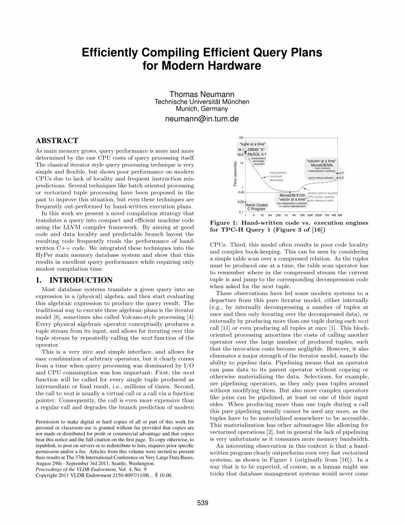
Figure 1: Hand-written code vs. execution enginesfor TPC-H Query 1 (Figure 3 of [16])

CPUs. Third, this model often results in poor code localityand complex book-keeping. This can be seen by consideringa simple table scan over a compressed relation. As the tuplesmust be produced one at a time, the table scan operator hasto remember where in the compressed stream the currenttuple is and jump to the corresponding decompression codewhen asked for the next tuple.

These observations have led some modern systems to adeparture from this pure iterator model, either internally(e.g., by internally decompressing a number of tuples atonce and then only iterating over the decompressed data), orexternally by producing more than one tuple during each nextcall [11] or even producing all tuples at once [1]. This block-oriented processing amortizes the costs of calling anotheroperator over the large number of produced tuples, suchthat the invocation costs become negligible. However, it alsoeliminates a major strength of the iterator model, namely theability to pipeline data. Pipelining means that an operatorcan pass data to its parent operator without copying orotherwise materializing the data. Selections, for example,are pipelining operators, as they only pass tuples aroundwithout modifying them. But also more complex operatorslike joins can be pipelined, at least on one of their inputsides. When producing more than one tuple during a callthis pure pipelining usually cannot be used any more, as thetuples have to be materialized somewhere to be accessible.This materialization has other advantages like allowing forvectorized operations [2], but in general the lack of pipeliningis very unfortunate as it consumes more memory bandwidth.

An interesting observation in this context is that a hand-written program clearly outperforms even very fast vectorizedsystems, as shown in Figure 1 (originally from [16]). In away that is to be expected, of course, as a human might usetricks that database management systems would never come

539

up with. On the other hand the query in this figure is asimple aggregation query, and one would expect that thereis only one reasonable way to evaluate this query. Thereforethe existing query evaluation schemes seem to be clearlysuboptimal.

The algebraic operator model is very useful for reasoningover the query, but it is not necessarily a good idea to exhibitthe operator structure during query processing itself. In thispaper we therefore propose a query compilation strategy thatdiffers from existing approaches in several important ways:

1. Processing is data centric and not operator centric.Data is processed such that we can keep it in CPUregisters as long as possible. Operator boundaries areblurred to achieve this goal.

2. Data is not pulled by operators but pushed towardsthe operators. This results in much better code anddata locality.

3. Queries are compiled into native machine code usingthe optimizing LLVM compiler framework [7].

The overall framework produces code that is very friendly tomodern CPU architectures and, as a result, rivals the speedof hand-coded query execution plans. In some cases we caneven outperform hand-written code, as using the LLVM as-sembly language allows for some tricks that are hard to do ina high-level programming language like C++. Furthermore,by using an established compiler framework, we benefit fromfuture compiler, code optimization, and hardware improve-ments, whereas other approaches that integrate processingoptimizations into the query engine itself will have to updatetheir systems manually. We demonstrate the impact of thesetechniques by integrating them into the HyPer main-memorydatabase management system [5] and performing variouscomparisons with other systems.

The rest of this paper is structured as follows: We firstdiscuss related work in Section 2. We then explain the overallarchitecture of our compilation framework in Section 3. Theactual code generation for algebraic operators is discussed inmore details in Section 4. We explain how different advancedprocessing techniques can be integrated into the frameworkin Section 5. We then show an extensive evaluation of ourtechniques in Section 6 and draw conclusions in Section 7.

2. RELATED WORKThe classical iterator model for query evaluation was pro-

posed quite early [8], and was made popular by the Volcanosystem [4]. Today, it is the most commonly used executionstrategy, as it is flexible and quite simple. As long as queryprocessing was dominated by disk I/O the iterator modelworked fine. However, as the CPU consumption became anissue, some systems tried to reduce the high calling costsof the iterator model by passing blocks of tuples betweenoperators [11]. This greatly reduces the number of functioninvocations, but causes additional materialization costs.

Modern main-memory database systems look at the prob-lem again, as for them CPU costs is a critical issue. TheMonetDB system [1, 9] goes to the other extreme, and mate-rializes all intermediate results, which eliminates the needto call an input operator repeatedly. Besides simplifyingoperator interaction, materialization has other advantages,too, but it also causes significant costs. The MonetDB/X100system [1] (which evolved into VectorWise) selected a mid-dle ground by passing large vectors of data and evaluatingqueries in a vectorized manner on each chunk. This offers

excellent performance, but, as shown in Figure 1, still doesnot reach the speed of hand-written code.

Another way to improve query processing is to compilethe query into some kind of executable format, instead ofusing interpreter structures. In [13] the authors proposedcompiling the query logic into Java Bytecode, which allowsfor using the Java JVM. However this is relatively heavyweight, and they still use the iterator model, which limitsthe benefits. Recent work on the HIQUE system proposedcompiling the query into C code using code templates foreach operator [6]. HIQUE eliminates the iterator model byinlining result materialization inside the operator execution.However, contrary to our proposal, the operator boundariesare still clearly visible. Furthermore, the costs of compilingthe generated C code are quite high [6].

Besides these more general approaches, many individualtechniques have been proposed to speed up query processing.One important line of work is reducing the impact of branch-ing, where [14] showed how to combine conjunctive predicatessuch that the trade-off between number of branches and num-ber of evaluated predicates is optimal. Other work has lookedat processing individual expressions more efficiently by usingSIMD instructions [12, 15].

3. THE QUERY COMPILER3.1 Query Processing Architecture

We propose a very different architecture for query process-ing (and, accordingly, for query compilation). In order tomaximize the query processing performance we have to makesure that we maximize data and code locality. To illustratethis point, we first give a definition of pipeline-breaker thatis more restrictive than in standard database systems: Analgebraic operator is a pipeline breaker for a given input sideif it takes an incoming tuple out of the CPU registers. It isa full pipeline breaker if it materializes all incoming tuplesfrom this side before continuing processing.

This definition is slightly hand-waving, as a single tuplemight already be too large to fit into the available CPUregisters, but for now we pretend that we have a sufficientnumber of registers for all input attributes. We will lookat this in more detail in Section 4. The main point is thatwe consider spilling data to memory as a pipeline-breakingoperation. During query processing, all data should be keptin CPU registers as long as possible.

Now the question is, how can we organize query processingsuch that the data can be kept in CPU registers as long aspossible? The classical iterator model is clearly ill-suitedfor this, as tuples are passed via function calls to arbitraryfunctions – which always results in evicting the registercontents. The block-oriented execution models have fewerpasses across function boundaries, but they clearly also breakthe pipeline as they produce batches of tuples beyond registercapacity. In fact any iterator-style processing paradigm thatpulls data up from the input operators risks breaking thepipeline, as, by offering an iterator-base view, it has to offera linearized access interface to the output of an arbitrarilycomplex relational operator. Sometimes operators couldproduce a certain small number of output tuples togethercheaply, without need for copying.

We therefore reverse the direction of data flow control.Instead of pulling tuples up, we push them towards the con-sumer operators. While pushing tuples, we continue pushinguntil we reach the next pipeline-breaker. As a consequence,

540

select *from R1,R3,

(select R2.z,count(*)from R2where R2.y=3group by R2.z) R2

where R1.x=7 and R1.a=R3.b and R2.z=R3.c

Figure 2: Example Query

R1

R2 R3

x=7

y=3

z;count(*)

a=b

z=c

R1

R2 R3

x=7

y=3

z;count(*)

a=b

z=c

original with pipeline boundaries

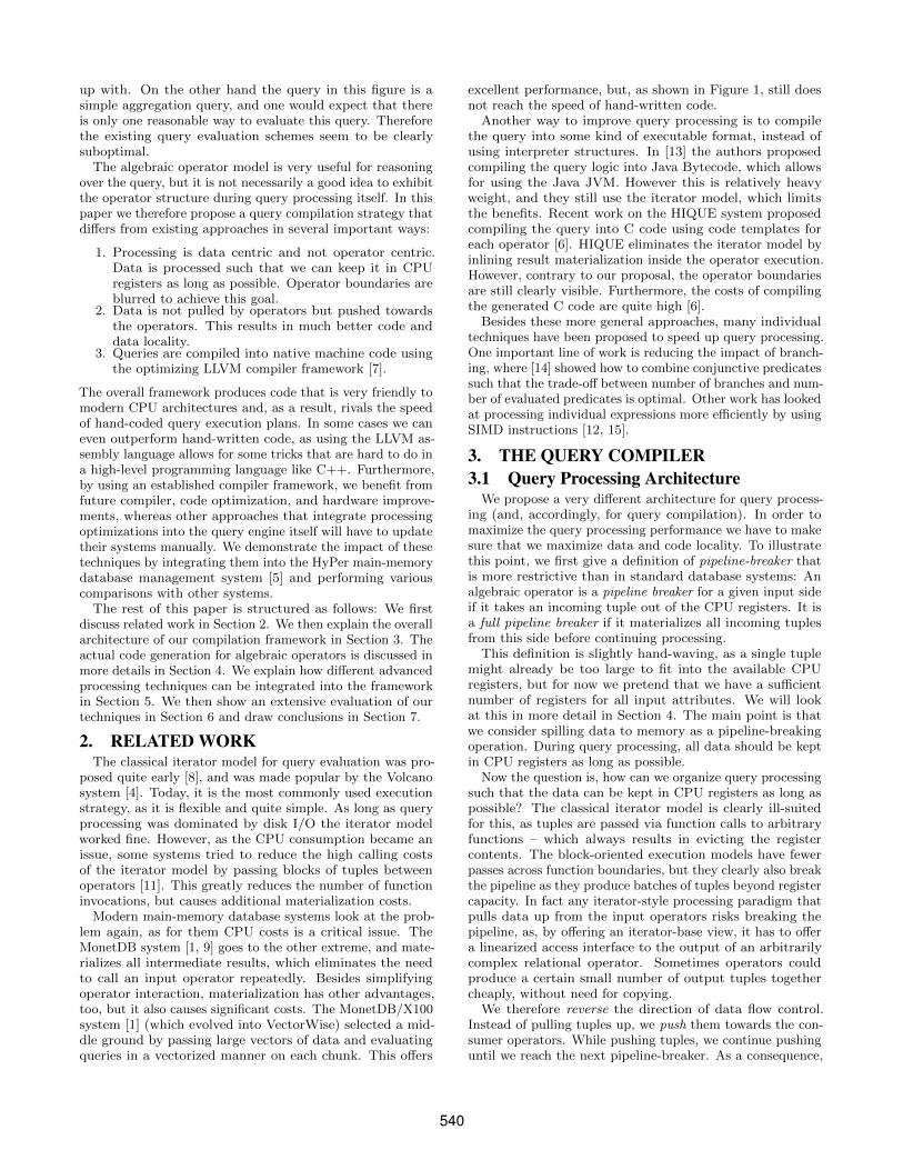
Figure 3: Example Execution Plan for Figure 2

data is always pushed from one pipeline-breaker into anotherpipeline-breaker. Operators in-between leave the tuples inCPU registers and are therefore very cheap to compute. Fur-thermore, in a push-based architecture the complex controlflow logic tends to be outside tight loops, which reducesregister pressure. As the typical pipeline-breakers wouldhave to materialize the tuples anyway, we produce executionplans that minimize the number of memory accesses.

As an illustrational example consider the execution plan inFigure 3 (Γ denotes a group by operator). The correspondingSQL query is shown in Figure 2. It selects some tuplesfrom R2, groups them by z, joins the result with R3, andjoins that result with some tuples from R1. In the classicaloperator model, the top-most join would produce tuples byfirst asking its left input for tuples repeatedly, placing each ofthem in a hash table, and then asking its right input for tuplesand probing the hash table for each table. The input sidesthemselves would operate in a similar manner recursively.When looking at the data flow in this example more carefully,we see that in principle the tuples are always passed from onematerialization point to another. The join a = b materializesthe tuples from its left input in a hash table, and receivesthem from a materialized state (namely from the scan of R1).The selection in between pipelines the tuples and performs nomaterialization. These materialization points (i.e., pipelineboundaries) are shown on the right hand side of Figure 3.

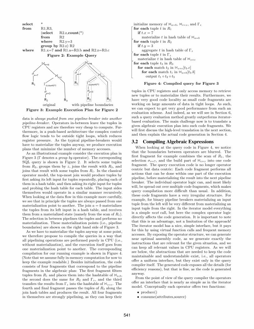
As we have to materialize the tuples anyway at some point,we therefore propose to compile the queries in a way thatall pipelining operations are performed purely in CPU (i.e.,without materialization), and the execution itself goes fromone materialization point to another. The correspondingcompilation for our running example is shown in Figure 4.(Note that we assume fully in-memory computation for now tokeep the example readable.) Besides initialization, the codeconsists of four fragments that correspond to the pipelinefragments in the algebraic plan: The first fragment filterstuples from R1 and places them into the hashtable of Ba,b,the second does the same for R2 and Γz, and the thirdtransfers the results from Γz into the hashtable of Bz=c. Thefourth and final fragment passes the tuples of R3 along thejoin hash tables and produces the result. All four fragmentsin themselves are strongly pipelining, as they can keep their

initialize memory of Ba=b, Bc=z, and Γz

for each tuple t in R1

if t.x = 7materialize t in hash table of Ba=b

for each tuple t in R2

if t.y = 3aggregate t in hash table of Γz

for each tuple t in Γz

materialize t in hash table of Bz=c

for each tuple t3 in R3

for each match t2 in Bz=c[t3.c]for each match t1 in Ba=b[t3.b]

output t1 ◦ t2 ◦ t3

Figure 4: Compiled query for Figure 3

tuples in CPU registers and only access memory to retrievenew tuples or to materialize their results. Furthermore, wehave very good code locality as small code fragments areworking on large amounts of data in tight loops. As such,we can expect to get very good performance from such anevaluation scheme. And indeed, as we will see in Section 6,such a query evaluation method greatly outperforms iterator-based evaluation. The main challenge now is to translate agiven algebraic execution plan into such code fragments. Wewill first discuss the high-level translation in the next section,and then explain the actual code generation in Section 4.

3.2 Compiling Algebraic ExpressionsWhen looking at the query code in Figure 4, we notice

that the boundaries between operators are blurred. Thefirst fragment for example combines the scan of R1, theselection σx=7, and the build part of Bc=z into one codefragment. The query execution code is no longer operatorcentric but data centric: Each code fragment performs allactions that can be done within one part of the executionpipeline, before materializing the result into the next pipelinebreaker. The individual operator logic can, and most likelywill, be spread out over multiple code fragments, which makesquery compilation more difficult than usual. In addition,these code fragments have a very irregular structure. Forexample, for binary pipeline breakers materializing an inputtuple from the left will be very different from materializing aninput tuple from the right. In the iterator model everythingis a simple next call, but here the complex operator logicdirectly affects the code generation. It is important to notethat this is an advantage, not a limitation of the approach!The iterator model has a nice, simple interface, but it paysfor this by using virtual function calls and frequent memoryaccesses. By exposing the operator structure, we can generatenear optimal assembly code, as we generate exactly theinstructions that are relevant for the given situation, and wecan keep all relevant values in CPU registers. As we willsee below, the abstractions that are needed to keep the codemaintainable and understandable exist, i.e., all operatorsoffer a uniform interface, but they exist only in the querycompiler itself. The generated code exposes all the details (forefficiency reasons), but that is fine, as the code is generatedanyway.

From the point of view of the query compiler the operatorsoffer an interface that is nearly as simple as in the iteratormodel. Conceptually each operator offers two functions:

• produce()• consume(attributes,source)

541

B.produce B.left.produce; B.right.produce;B.consume(a,s) if (s==B.left)

print “materialize tuple in hash table”;elseprint “for each match in hashtable[”

+a.joinattr+“]”;B.parent.consume(a+new attributes)

σ.produce σ.input.produceσ.consume(a,s) print “if ”+σ.condition;

σ.parent.consume(attr,σ)scan.produce print “for each tuple in relation”

scan.parent.consume(attributes,scan)

Figure 5: A simple translation scheme to illustratethe produce/consume interaction

Conceptually, the produce function asks the operator toproduce its result tuples, which are then pushed towards theconsuming operator by calling their consume functions. Forour running example, the query would be executed by callingBa=b.produce. This produce function would then in itself callσx=7.produce to fill its hash table, and the σ operator wouldcall R1.produce to access the relation. R1 is a leaf in theoperator tree, i.e., it can produce tuples on its own. Thereforeit scans the relation R1, and for each tuple loads the requiredattributes and calls σx=7.consume(attributes,R1) to handthe tuple to the selection. The selection filters the tuples, andif it qualifies it passes it by calling Ba=b(attributes, σx=7).The join sees that it gets tuples from the left side, and thusstores them in the hash table. After all tuples from R1 areproduced, the control flow goes back to the join, which willcall Bc=z.produce to get the tuples from the probe side etc.

However, this produce/consume interface is only a mentalmodel. These functions do not exist explicitly, they are onlyused by the code generation. When compiling an SQL query,the query is first processed as usual, i.e., the query is parsed,translated into algebra, and the algebraic expression is opti-mized. Only then do we deviate from the standard scheme.The final algebraic plan is not translated into physical al-gebra that can be executed, but instead compiled into animperative program. And only this compilation step uses theproduce/consume interface internally to produce the requiredimperative code. This code generation model is illustratedin Figure 5. It shows a very simple translation scheme thatconverts B, σ, and scans into pseudo-code. The readers canconvince themselves that applying the rules from Figure 5 tothe operator tree in Figure 3 will produce the pseudo-codefrom Figure 4 (except for differences in variable names andmemory initialization). The real translation code is signifi-cantly more complex, of course, as we have to keep track ofthe loaded attributes, the state of the operators involved, at-tribute dependencies in the case of correlated subqueries, etc.,but in principle this simple mapping already shows how wecan translate algebraic expressions into imperative code. Weinclude a more detailed operator translation in Appendix A.As these code fragments always operate on certain pieces ofdata at a time, thus having very good locality, the resultingcode proved to execute efficiently.

4. CODE GENERATION4.1 Generating Machine Code

So far we have only discussed the translation of algebraicexpressions into pseudo-code, but in practice we want tocompile the query into machine code. Initially we exper-

C++scan

C++

C++

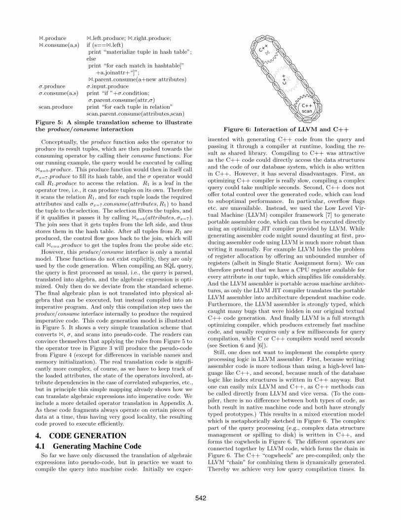
Figure 6: Interaction of LLVM and C++

imented with generating C++ code from the query andpassing it through a compiler at runtime, loading the re-sult as shared library. Compiling to C++ was attractiveas the C++ code could directly access the data structuresand the code of our database system, which is also writtenin C++. However, it has several disadvantages. First, anoptimizing C++ compiler is really slow, compiling a complexquery could take multiple seconds. Second, C++ does notoffer total control over the generated code, which can leadto suboptimal performance. In particular, overflow flagsetc. are unavailable. Instead, we used the Low Level Vir-tual Machine (LLVM) compiler framework [7] to generateportable assembler code, which can then be executed directlyusing an optimizing JIT compiler provided by LLVM. Whilegenerating assembler code might sound daunting at first, pro-ducing assembler code using LLVM is much more robust thanwriting it manually. For example LLVM hides the problemof register allocation by offering an unbounded number ofregisters (albeit in Single Static Assignment form). We cantherefore pretend that we have a CPU register available forevery attribute in our tuple, which simplifies life considerably.And the LLVM assembler is portable across machine architec-tures, as only the LLVM JIT compiler translates the portableLLVM assembler into architecture dependent machine code.Furthermore, the LLVM assembler is strongly typed, whichcaught many bugs that were hidden in our original textualC++ code generation. And finally LLVM is a full strengthoptimizing compiler, which produces extremely fast machinecode, and usually requires only a few milliseconds for querycompilation, while C or C++ compilers would need seconds(see Section 6 and [6]).

Still, one does not want to implement the complete queryprocessing logic in LLVM assembler. First, because writingassembler code is more tedious than using a high-level lan-guage like C++, and second, because much of the databaselogic like index structures is written in C++ anyway. Butone can easily mix LLVM and C++, as C++ methods canbe called directly from LLVM and vice versa. (To the com-piler, there is no difference between both types of code, asboth result in native machine code and both have stronglytyped prototypes.) This results in a mixed execution modelwhich is metaphorically sketched in Figure 6. The complexpart of the query processing (e.g., complex data structuremanagement or spilling to disk) is written in C++, andforms the cogwheels in Figure 6. The different operators areconnected together by LLVM code, which forms the chain inFigure 6. The C++ “cogwheels” are pre-compiled; only theLLVM “chain” for combining them is dynamically generated.Thereby we achieve very low query compilation times. In

542

the concrete example, the complex part of the scan (e.g.,locating data structures, figuring out what to scan next)is implemented in C++, and this C++ code “drives” theexecution pipeline. But the tuple access itself and the furthertuple processing (filtering, materialization in hash table) isimplemented in LLVM assembler code. C++ code is calledfrom time to time (like when allocating more memory), butinteraction of the C++ parts is controlled by LLVM. If com-plex operators like sort are involved, control might go backfully into C++ at some point, but once the complex logic isover and tuples have to be processed in bulk, LLVM takesover again. For optimal performance it is important thatthe hot path, i.e., the code that is executed for 99% of thetuples, is pure LLVM. Calling C++ from time to time (e.g.,when switching to a new page) is fine, the costs for that arenegligible, but the bulk of the processing has to be done inLLVM. While staying in LLVM, we can keep the tuples inCPU registers all the time, which is about as fast as we canexpect to be. When calling an external function all registershave to be spilled to memory, which is somewhat expensive.In absolute terms it is very cheap, of course, as the registerswill be spilled on the stack, which is usually in cache, but ifthis is done millions of times it becomes noticeable.

4.2 Complex OperatorsWhile code generation for scans and selections is more or

less straightforward, some care is needed when generatingcode for more complex operators like sort or join. The firstthing to keep in mind is that contrary to the simple examplesseen so far in the paper it is not possible or even desirableto compile a complex query into a single function. This hasmultiple reasons. First, there is the pragmatic reason thatthe LLVM code will most likely call C++ code at some pointthat will take over the control flow. For example an externalsorting operator will produce the initial runs with LLVM,but will probably control the merge phase from within C++,calling LLVM functions as needed. The second reason is thatinlining the complete query logic into a single function canlead to an exponential growth in code. For example outerjoins will call their consumers in two different situations, firstwhen they have found a match, and second, when producingNULL values. One could directly include the consumer codein both cases, but then a cascade of outer joins would lead toan exponential growth in code. Therefore it makes sense todefine functions within LLVM itself, that can then be calledfrom places within the LLVM code. Again, one has to makesure that the hot path does not cross a function boundary.Thus a pipelining fragment of the algebraic expression shouldresult in one compact LLVM code fragment.

This need for multiple functions affects the way that wegenerate code. In particular, we have to keep track of allattributes and remember if they are currently available inregisters. Materializing attributes in memory is a deliberatedecision, similar to spooling tuples to disk. Of course notfrom a performance point of view, materializing in memory isrelatively fast, but from a code point of view materializationis a very complex step that should be avoided if possible.

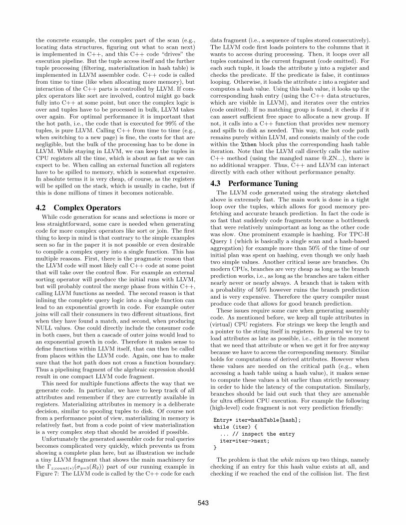
Unfortunately the generated assembler code for real queriesbecomes complicated very quickly, which prevents us fromshowing a complete plan here, but as illustration we includea tiny LLVM fragment that shows the main machinery forthe Γz;count(∗)(σy=3(R2)) part of our running example inFigure 7: The LLVM code is called by the C++ code for each

data fragment (i.e., a sequence of tuples stored consecutively).The LLVM code first loads pointers to the columns that itwants to access during processing. Then, it loops over alltuples contained in the current fragment (code omitted). Foreach such tuple, it loads the attribute y into a register andchecks the predicate. If the predicate is false, it continueslooping. Otherwise, it loads the attribute z into a register andcomputes a hash value. Using this hash value, it looks up thecorresponding hash entry (using the C++ data structures,which are visible in LLVM), and iterates over the entries(code omitted). If no matching group is found, it checks if itcan assert sufficient free space to allocate a new group. Ifnot, it calls into a C++ function that provides new memoryand spills to disk as needed. This way, the hot code pathremains purely within LLVM, and consists mainly of the codewithin the %then block plus the corresponding hash tableiteration. Note that the LLVM call directly calls the nativeC++ method (using the mangled name @ ZN...), there isno additional wrapper. Thus, C++ and LLVM can interactdirectly with each other without performance penalty.

4.3 Performance TuningThe LLVM code generated using the strategy sketched

above is extremely fast. The main work is done in a tightloop over the tuples, which allows for good memory pre-fetching and accurate branch prediction. In fact the code isso fast that suddenly code fragments become a bottleneckthat were relatively unimportant as long as the other codewas slow. One prominent example is hashing. For TPC-HQuery 1 (which is basically a single scan and a hash-basedaggregation) for example more than 50% of the time of ourinitial plan was spent on hashing, even though we only hashtwo simple values. Another critical issue are branches. Onmodern CPUs, branches are very cheap as long as the branchprediction works, i.e., as long as the branches are taken eithernearly never or nearly always. A branch that is taken witha probability of 50% however ruins the branch predictionand is very expensive. Therefore the query compiler mustproduce code that allows for good branch prediction.

These issues require some care when generating assemblycode. As mentioned before, we keep all tuple attributes in(virtual) CPU registers. For strings we keep the length anda pointer to the string itself in registers. In general we try toload attributes as late as possible, i.e., either in the momentthat we need that attribute or when we get it for free anywaybecause we have to access the corresponding memory. Similarholds for computations of derived attributes. However whenthese values are needed on the critical path (e.g., whenaccessing a hash table using a hash value), it makes senseto compute these values a bit earlier than strictly necessaryin order to hide the latency of the computation. Similarly,branches should be laid out such that they are amenablefor ultra efficient CPU execution. For example the following(high-level) code fragment is not very prediction friendly:

Entry* iter=hashTable[hash];

while (iter) {

... // inspect the entry

iter=iter->next;

}

The problem is that the while mixes up two things, namelychecking if an entry for this hash value exists at all, andchecking if we reached the end of the collision list. The first

543

1. locate tuples in memory

2. loop over all tuples

3. filter y = 3

4. hash z

5. lookup in hash table (C++ data structure)

6. not found, check space

7. full, call C++ to allocate mem or spill

define internal void @scanConsumer(%8∗ %executionState, %Fragment R2∗ %data) {body:

...%columnPtr = getelementptr inbounds %Fragment R2∗ %data, i32 0, i32 0%column = load i32∗∗ %columnPtr, align 8%columnPtr2 = getelementptr inbounds %Fragment R2∗ %data, i32 0, i32 1%column2 = load i32∗∗ %columnPtr2, align 8... (loop over tuples , currently at %id, contains label %cont17)%yPtr = getelementptr i32∗ %column, i64 %id%y = load i32∗ %yPtr, align 4%cond = icmp eq i32 %y, 3br i1 %cond, label %then, label %cont17

then:%zPtr = getelementptr i32∗ %column2, i64 %id%z = load i32∗ %zPtr, align 4%hash = urem i32 %z, %hashTableSize%hashSlot = getelementptr %”HashGroupify::Entry”∗∗ %hashTable, i32 %hash%hashIter = load %”HashGroupify::Entry”∗∗ %hashSlot, align 8%cond2 = icmp eq %”HashGroupify::Entry”∗ %hashIter, nullbr i1 %cond, label %loop20, label %else26... (check if the group already exists , starts with label %loop20)

else26 :%cond3 = icmp le i32 %spaceRemaining, i32 8br i1 %cond, label %then28, label %else47... (create a new group, starts with label %then28)

else47 :%ptr = call i8∗ @ ZN12HashGroupify15storeInputTupleEmj

(%”HashGroupify”∗ %1, i32 hash, i32 8)... (more loop logic)

}

Figure 7: LLVM fragment for the first steps of the query Γz;count(∗)(σy=3(R2))

case will nearly always be true, as we expect the hash tableto be filled, while the second case will nearly always be false,as our collision lists are very short. Therefore, the followingcode fragment is more prediction friendly:

Entry* iter=hashTable[hash];

if (iter) do {

... // inspect the entry

iter=iter->next;

} while (iter);

Of course our code uses LLVM branches and not C++loops, but the same is true there, branch prediction improvessignificantly when producing code like this. And this codelayout has a noticeable impact on query processing, in ourexperiments just changing the branch structure improvedhash table lookups by more than 20%.

All these issues complicate code generation, of course. Butoverall the effort required to avoid these pitfalls is not toosevere. The LLVM code is generated anyway, and spendingeffort on the code generator once will pay off for all sub-sequent queries. The code generator is relatively compact.In our implementation the code generation for all algebraicoperators required for SQL-92 consists of about 11,000 linesof code, which is not a lot.

5. ADVANCED PARALLELIZATION TECH-NIQUES

In the previous sections we have discussed how to compilequeries into data-centric execution programs. By organizingthe data flow and the control flow such that tuples arepushed directly from one pipeline breaker into another, andby keeping data in registers as long as possible, we getexcellent data locality. However, this does not mean that

we have to process tuples linearly, one tuple at a time. Ourinitial implementation pushes individual tuples, and thisalready performs very well, but more advanced processingtechniques can be integrated very naturally in the generalframework. We now look at several of them.

Traditional block-wise processing [11] has the great disad-vantage of creating additional memory accesses. However,processing more than one tuple at once is indeed a very goodidea, as long as we can keep the whole block in registers. Inparticular when using SIMD registers this is often the case.Processing more than one tuple at a time has several advan-tages: First, of course, it allows for using SIMD instructionson modern CPUs [15], which can greatly speed up processing.Second, it can help delay branching, as predicates can beevaluated and combined without executing branches immedi-ately [12, 14]. Strictly speaking the techniques from [14] arevery useful already for individual tuples, but the effect can beeven larger for blocks of tuples. This style of block process-ing where values are packed into a (large) register fits verynaturally into our framework, as the operators always passregister values to their consumers. LLVM directly allows formodeling SIMD values as vector types, thus the impact onthe overall code generation framework are relatively minor.

SIMD instructions are a kind of inter-tuple parallelism,i.e., processing multiple tuples with one instruction. Thesecond kind of parallelism relevant for modern CPUs is multi-core processing. Nearly all database systems will exploitmulti-core architectures for inter-query parallelism, but asthe number of cores available on modern CPUs increases,intra-query parallelism becomes more important. In prin-ciple this is a well studied problem [10, 3], and is usuallysolved by partitioning the input of operators, processingeach partition independently, and then merging the resultsfrom all partitions. For our code generation framework this

544

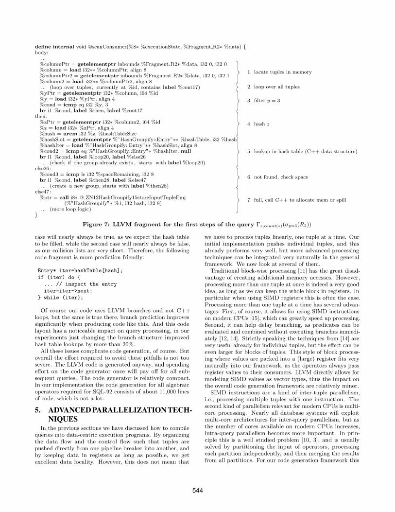
HyPer + C++ HyPer + LLVMTPC-C [tps] 161,794 169,491total compile time [s] 16.53 0.81

Table 1: OLTP Performance of Different Engines

kind of parallelism can be supported with nearly no codechanges. As illustrated in Figure 7, the code always operateson fragments of data, that are processed in a tight loop, andmaterialized into the next pipeline breaker. Usually, thefragments are determined by the storage system, but theycould as well come from a parallelizing decision. Only someadditional logic would be required to merge the individualresults. Note that the “parallelizing decision” in itself isa difficult problem! Spitting and merging data streams isexpensive, and the optimizer has to be careful about intro-ducing parallelism. This is beyond the scope of this paper.But for future work it is a very relevant problem, as thenumber of cores is increasing.

6. EVALUATIONWe have implemented the techniques proposed in this pa-

per both in the HyPer main-memory database managementsystems [5], and in a disk-based DBMS. We found that thetechniques work excellent, both when operating purely inmemory and when spooling to disk if needed. However itis difficult to precisely measure the impact our compilationtechniques have relative to other approaches, as query per-formance is greatly affected by other effects like differencesin storage systems, too. The evaluation is therefore split intotwo parts: We include a full systems comparison here, includ-ing an analysis of the generated code. A microbenchmarkfor specific operator behavior is included in Appendix B.

In the system comparison we include experiments run onMonetDB 1.36.5, Ingres VectorWise 1.0, and a commercialdatabase system we shall call DB X. All experiments wereconducted on a Dual Intel X5570 Quad-Core-CPU with64GB main memory, Red Hat Enterprise Linux 5.4. OurC++ code was compiled using gcc 4.5.2, and the machinecode was produced using LLVM 2.8. The optimization levelsare explained in more detail in Appendix C.

6.1 Systems ComparisonThe HyPer system in which we integrated our query com-

pilation techniques is designed as a hybrid OLTP and OLAPsystem, i.e., it can handle both kinds of workloads concur-rently. We therefore used the TPC-CH benchmark from[5] for experiments. For the OLTP side it runs a TPC-Cbenchmark, and for the OLAP side it executes the 22 TPC-Hqueries adapted to the (slightly extended) TPC-C schema.The first five queries are included in Appendix D. As we aremainly interested in an evaluation of raw query processingspeed here, we ran a setup without concurrency, i.e., weloaded 12 warehouses, and then executed the TPC-C trans-actions single-threaded and without client wait times. Simi-larly the OLAP queries are executed on the 12 warehousessingle-threaded and without concurrent updates. What isinteresting for the comparison is that HyPer originally com-piled the queries into C++ code using hand-written codefragments, which allows us to estimate the impact LLVMhas relative to C++ code.

We ran the OLTP part only in HyPer, as the other sys-tems were not designed for OLTP workloads. The results

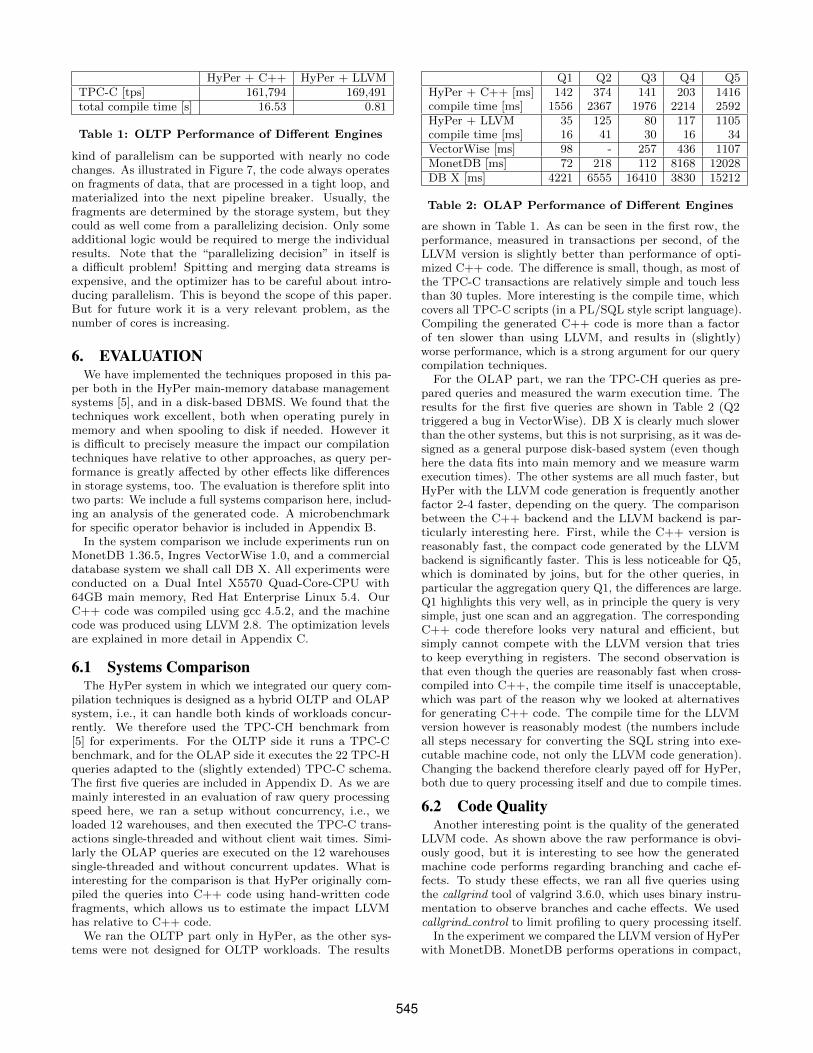
Q1 Q2 Q3 Q4 Q5HyPer + C++ [ms] 142 374 141 203 1416compile time [ms] 1556 2367 1976 2214 2592HyPer + LLVM 35 125 80 117 1105compile time [ms] 16 41 30 16 34VectorWise [ms] 98 - 257 436 1107MonetDB [ms] 72 218 112 8168 12028DB X [ms] 4221 6555 16410 3830 15212

Table 2: OLAP Performance of Different Engines

are shown in Table 1. As can be seen in the first row, theperformance, measured in transactions per second, of theLLVM version is slightly better than performance of opti-mized C++ code. The difference is small, though, as most ofthe TPC-C transactions are relatively simple and touch lessthan 30 tuples. More interesting is the compile time, whichcovers all TPC-C scripts (in a PL/SQL style script language).Compiling the generated C++ code is more than a factorof ten slower than using LLVM, and results in (slightly)worse performance, which is a strong argument for our querycompilation techniques.

For the OLAP part, we ran the TPC-CH queries as pre-pared queries and measured the warm execution time. Theresults for the first five queries are shown in Table 2 (Q2triggered a bug in VectorWise). DB X is clearly much slowerthan the other systems, but this is not surprising, as it was de-signed as a general purpose disk-based system (even thoughhere the data fits into main memory and we measure warmexecution times). The other systems are all much faster, butHyPer with the LLVM code generation is frequently anotherfactor 2-4 faster, depending on the query. The comparisonbetween the C++ backend and the LLVM backend is par-ticularly interesting here. First, while the C++ version isreasonably fast, the compact code generated by the LLVMbackend is significantly faster. This is less noticeable for Q5,which is dominated by joins, but for the other queries, inparticular the aggregation query Q1, the differences are large.Q1 highlights this very well, as in principle the query is verysimple, just one scan and an aggregation. The correspondingC++ code therefore looks very natural and efficient, butsimply cannot compete with the LLVM version that triesto keep everything in registers. The second observation isthat even though the queries are reasonably fast when cross-compiled into C++, the compile time itself is unacceptable,which was part of the reason why we looked at alternativesfor generating C++ code. The compile time for the LLVMversion however is reasonably modest (the numbers includeall steps necessary for converting the SQL string into exe-cutable machine code, not only the LLVM code generation).Changing the backend therefore clearly payed off for HyPer,both due to query processing itself and due to compile times.

6.2 Code QualityAnother interesting point is the quality of the generated

LLVM code. As shown above the raw performance is obvi-ously good, but it is interesting to see how the generatedmachine code performs regarding branching and cache ef-fects. To study these effects, we ran all five queries usingthe callgrind tool of valgrind 3.6.0, which uses binary instru-mentation to observe branches and cache effects. We usedcallgrind control to limit profiling to query processing itself.

In the experiment we compared the LLVM version of HyPerwith MonetDB. MonetDB performs operations in compact,

545

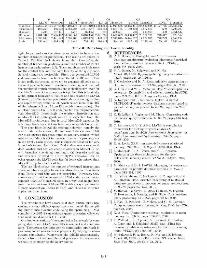
Q1 Q2 Q3 Q4 Q5LLVM MonetDB LLVM MonetDB LLVM MonetDB LLVM MonetDB LLVM MonetDB

branches 19,765,048 144,557,672 37,409,113 114,584,910 14,362,660 127,944,656 32,243,391 408,891,838 11,427,746 333,536,532mispredicts 188,260 456,078 6,581,223 3,891,827 696,839 1,884,185 1,182,202 6,577,871 639 6,726,700I1 misses 2,793 187,471 1,778 146,305 791 386,561 508 290,894 490 2,061,837D1 misses 1,764,937 7,545,432 10,068,857 6,610,366 2,341,531 7,557,629 3,480,437 20,981,731 776,417 8,573,962L2d misses 1,689,163 7,341,140 7,539,400 4,012,969 1,420,628 5,947,845 3,424,857 17,072,319 776,229 7,552,794I refs 132 mil 1,184 mil 313 mil 760 mil 208 mil 944 mil 282 mil 3,140 mil 159 mil 2,089 mil

Table 3: Branching and Cache Locality

tight loops, and can therefore be expected to have a lownumber of branch mispredictions. The results are shown inTable 3. The first block shows the number of branches, thenumber of branch mispredictions, and the number of level 1instruction cache misses (I1). These numbers are indicatorsfor the control flow and the code locality of the query code.Several things are noticeable. First, our generated LLVMcode contains far less branches than the MonetDB code. Thisis not really surprising, as we try to generate all code up tothe next pipeline breaker in one linear code fragment. Second,the number of branch mispredictions is significantly lower forthe LLVM code. One exception is Q2, but this is basicallya sub-optimal behavior of HyPer and not related to LLVM.(Currently HyPer is very pessimistic about spooling to disc,and copies strings around a lot, which causes more than 60%of the mispredictions. MonetDB avoids these copies). Forall other queries the LLVM code has far less mispredictionsthan MonetDB. Interestingly the relative misprediction rateof MonetDB is quite good, as can be expected from theMonetDB architecture, but in total MonetDB executes fartoo many branches and thus has many mispredictions, too.

The next block shows the caching behavior, namely thelevel 1 data cache misses (D1) and level 2 data misses (L2d).For most queries these two numbers are very similar, whichmeans that if data is not in the level 1 cache it is probably notin the level 2 cache either. This is expected behavior for verylarge hash tables. Again the LLVM code shows a very gooddata locality and has less cache misses than MonetDB. Aswith branches, the string handling in Q2 degrades caching,but this will be fixed in future HyPer versions. For allother queries the LLVM code has far less cache misses thanMonetDB, up to a factor of ten.

The last block shows the number of executed instructions.These numbers roughly follow the absolute execution timesfrom Table 2 and thus are not surprising. However, theyshow clearly that the generated LLVM code is much morecompact than the MonetDB code. In a way that might stemfrom the architecture of MonetDB which always operates onBinary Association Tables (BATs), and thus has to touchtuples multiple times.

7. CONCLUSIONThe experiments have shown that data-centric query pro-

cessing is a very efficient query execution model. By compil-ing queries into machine code using the optimizing LLVMcompiler, the DBMS can achieve a query processing efficiencythat rivals hand-written C++ code.

Our implementation of the compilation framework for com-piling algebra into LLVM assembler is compact and maintain-able. Thereforem the data-centric compilation approach ispromising for all new database projects. By relying on main-stream compilation frameworks the DBMS automaticallybenefits from future compiler and processor improvementswithout re-engineering the query engine.

8. REFERENCES[1] P. A. Boncz, S. Manegold, and M. L. Kersten.

Database architecture evolution: Mammals flourishedlong before dinosaurs became extinct. PVLDB,2(2):1648–1653, 2009.

[2] P. A. Boncz, M. Zukowski, and N. Nes.MonetDB/X100: Hyper-pipelining query execution. InCIDR, pages 225–237, 2005.

[3] J. Cieslewicz and K. A. Ross. Adaptive aggregation onchip multiprocessors. In VLDB, pages 339–350, 2007.

[4] G. Graefe and W. J. McKenna. The Volcano optimizergenerator: Extensibility and efficient search. In ICDE,pages 209–218. IEEE Computer Society, 1993.

[5] A. Kemper and T. Neumann. HyPer: A hybridOLTP&OLAP main memory database system based onvirtual memory snapshots. In ICDE, pages 195–206,2011.

[6] K. Krikellas, S. Viglas, and M. Cintra. Generating codefor holistic query evaluation. In ICDE, pages 613–624,2010.

[7] C. Lattner and V. S. Adve. LLVM: A compilationframework for lifelong program analysis &transformation. In ACM International Symposium onCode Generation and Optimization (CGO), pages75–88, 2004.

[8] R. A. Lorie. XRM - an extended (n-ary) relationalmemory. IBM Research Report, G320-2096, 1974.

[9] S. Manegold, P. A. Boncz, and M. L. Kersten.Optimizing database architecture for the newbottleneck: memory access. VLDB J., 9(3):231–246,2000.

[10] M. Mehta and D. J. DeWitt. Managing intra-operatorparallelism in parallel database systems. In VLDB,pages 382–394, 1995.

[11] S. Padmanabhan, T. Malkemus, R. C. Agarwal, andA. Jhingran. Block oriented processing of relationaldatabase operations in modern computer architectures.In ICDE, pages 567–574, 2001.

[12] V. Raman, G. Swart, L. Qiao, F. Reiss, V. Dialani,D. Kossmann, I. Narang, and R. Sidle. Constant-timequery processing. In ICDE, pages 60–69, 2008.

[13] J. Rao, H. Pirahesh, C. Mohan, and G. M. Lohman.Compiled query execution engine using JVM. In ICDE,page 23, 2006.

[14] K. A. Ross. Conjunctive selection conditions in mainmemory. In PODS, pages 109–120, 2002.

[15] T. Willhalm, N. Popovici, Y. Boshmaf, H. Plattner,A. Zeier, and J. Schaffner. SIMD-scan: Ultra fastin-memory table scan using on-chip vector processingunits. PVLDB, 2(1):385–394, 2009.

[16] M. Zukowski, P. A. Boncz, N. Nes, and S. Heman.MonetDB/X100 - a DBMS in the CPU cache. IEEEData Eng. Bull., 28(2):17–22, 2005.

546

APPENDIXA. OPERATOR TRANSLATION

Due to space constraints we could only give a high-levelaccount of operator translation in Section 3, and includea more detailed discussion here. We concentrate on theoperators Scan, Select, Project, Map, and HashJoin here, asthese are sufficient to translate a wide class of queries. Thefirst four operators are quite simple, and illustrate the basicproduce/consume interaction, while the hash join is muchmore involved.

The query compilation maintains quite a bit of infrastruc-ture that is passed around during operator translation. Themost important objects are codegen, which offers an interfaceto the LLVM code generation (operator-> is overloaded toaccess IRBuilder from LLVM), context, which keeps track ofavailable attributes (both from input operators and, for cor-related subqeueries, from “outside”), and getParent, whichreturns the parent operator. In addition, helper objects areused to automate LLVM code generation tasks. In particularLoop and If are used to automate control flow.

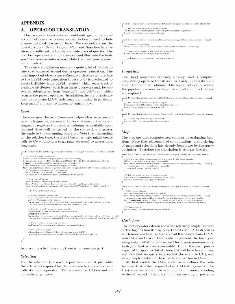
ScanThe scan uses the ScanConsumer helper class to access allrelation fragments, accesses all tuples contained in the currentfragment, registers the required columns as available upondemand (they will be cached by the context), and passesthe tuple to the consuming operator. Note that, dependingon the relation type, the ScanConsumer logic might createcalls to C++ functions (e.g., page accesses) to access datafragments.

void TableScanTranslator::produce(CodeGen& codegen,Context& context) const{

// Access all relation fragmentsllvm::Value∗ dbPtr=codegen.getDatabasePointer();llvm::Value∗ relationPtr=codegen.getPtr(dbPtr,db.layout.relations[table]);auto& required=scanConsumer.getPartitionPtr();ScanConsumer scanConsumer(codegen,context)for (;db.relations[table]−>generateScan(codegen,relationPtr,scanConsumer);) {

// Prepare accessing the current fragmentllvm::Value∗ partitionPtr=required;ColumnAccess columnAccess(partitionPtr,required);

// Loop over all tuplesllvm::Value∗ tid=codegen.const64(0);llvm::Value∗ limit=codegen.load(partitionPtr,getLayout().size);Loop loop(codegen,codegen−>CreateICmpULT(tid,limit),{{tid,”tid”}});{

tid=loop.getLoopVar(0);

// Prepare column access codePartitionAccess::ColumnAccess::Row rowAccess(columnAccess,tid);vector<ValueAccess> access;for (auto iter=required.begin(),limit=required.end();iter!=limit;++iter)

access.push back(rowAccess.loadAttribute(∗iter));

// Register providers in new inner contextConsumerContext consumerContext(context);unsigned slot=0;for (auto iter=required.begin(),limit=required.end();iter!=limit;++iter,++slot)

consumerContext.registerIUProvider(&(getOutput()[∗iter].iu),&access[slot]);

// Push results to consuming operatorsgetParent()−>consume(codegen,consumerContext);

// Go to the next tupletid=codegen−>CreateAdd(tid,codegen.const64(1));loop.loopDone(codegen−>CreateICmpULT(tid,limit),{tid});}}}

As a scan is a leaf operator, there is no consume part.

SelectionFor the selection the produce part is simple, it just addsthe attributes required for the predicate to the context andcalls its input operator. The consume part filters out allnon-satisfying tuples.

void SelectTranslator::produce(CodeGen& codegen,Context& context) const{

// Ask the input operator to produce tuplesAddRequired addRequired(context,getCondition().getUsed());input−>produce(codegen,context);}

void SelectTranslator::consume(CodeGen& codegen,Context& context) const{

// Evaluate the predicateResultValue value=codegen.deriveValue(getCondition(),context);

// Pass tuple to parent if the predicate is satisfiedCodeGen::If checkCond(codegen,value);{

getParent()−>consume(codegen,context);}}

ProjectionThe (bag) projection is nearly a no-op, and is compiledaway during operator translation, as it only informs its inputabout the required columns. The real effect occurs withinthe pipeline breakers, as they discard all columns that arenot required.

void ProjectTranslator::produce(CodeGen& codegen,Context& context) const{

// Ask the input operator to produce tuplesSetRequired setRequired(context,getOutput());input−>produce(codegen,context);}

void ProjectTranslator::consume(CodeGen& codegen,Context& context) const{

// No code required here, pass to parentgetParent()−>consume(codegen,context);}

MapThe map operator computes new columns by evaluating func-tions. Note that placement of computations, and orderingof maps and selections has already been done by the queryoptimizer. Therefore the translation is straight forward.

void MapTranslator::produce(CodeGen& codegen,Context& context) const{

// Figure out which columns have to be provided by the input operatorIUSet required=context.getRequired();for (auto iter=functions.begin(),limit=functions.end();iter!=limit;++iter) {

(∗iter).function−>getUsed(required);required.erase((∗iter).result);}

// Ask the input operator to produce tuplesSetRequired setRequired(context,required);input−>produce(codegen,context);}

void MapTranslator::consume(CodeGen& codegen,Context& context) const{

// Offer new columnsvector<ExpressionAccess> accessors;for (auto iter=functions.begin(),limit=functions.end();iter!=limit;++iter)

accessors.push back(ExpressionAccess(codegen,∗(∗iter).function));for (unsigned index=0,limit=accessors.size();index<limit;index++)

context.registerIUProvider(functions[index].result,&accessors[index]);

// Pass to parentgetParent()−>consume(codegen,context);}

Hash JoinThe four operators shown above are relatively simple, as mostof the logic is handled by pure LLVM code. A hash join ismuch more involved, as here control flow moves from LLVMinto C++ and back. One could implement the hash joinusing only LLVM, of course, and for a pure main-memoryhash join that is even reasonable. But if the hash join isexpected to spool to disk if needed, it will have to call manymethods that are query independent (for example I/O), andin our implementation these parts are written in C++.

We first sketch the C++ code, as it defines the codetemplate that is then augmented with LLVM fragments. TheC++ code loads the build side into main memory, spoolingto disk if needed. If data fits into main memory, it just joins

547

with the probe side. Otherwise, it spools the probe side intopartitions, too, and joins the partitions. For simplicity welimit ourselves to inner joins here, non-inner joins requireadditional bookkeeping to remember which tuples have beenjoined.

void HashJoin::Inner::produce(){

// Read the build sideinitMem();produceLeft();if (inMem) {

buildHashTable();} else {

// Spool remaining tuples to diskspoolLeft();finishSpoolLeft();}

// Is a in−memory join possible?if (inMem) {

produceRight();return;}

// No, spool the right hand side, toospoolRight();

// Grace hash joinloadPartition(0);while (true) {

// More tuples on the right?for (;rightScanRemaining;) {

const void∗ rightTuple=nextRight();for (LookupHash lookup(rightTuple);lookup;++lookup) {

join(lookup.data(),rightTuple);}}

// Handle overflow in n:m caseif (overflow) {

loadPartitionLeft();resetRightScan();continue;}

// Go to the next partitionif ((++inMemPartition)>=partitionCount) {

return;} else {

loadPartition(inMemPartition);}}}

Thus the LLVM code has to provide three functions: pro-duce/consume as before, and an additional join function thatthe C++ code can call directly when joining tuples thathad been spooled to disk. Note that in this case the hashtable lookups etc. are already implemented in C++, so joinis only called for likely join candidates. The produce func-tion simply passes the control flow to the C++ code. Theconsume functions (one for each join side) hashes the joinvalues, determines the relevant registers, and materializesthem into the hash table. Note that for performance reasonsthe HyPer system skips the in-memory materialization ofthe right hand side and directly probes the hash table if nodata was spooled to disk, but this was omitted here due tospace constraints.

void HJTranslatorInner::produce(CodeGen& codegen,Context& context) const{

// Construct functions that will be be called from the C++ code{

AddRequired addRequired(context,getCondiution().getUsed().limitTo(left));produceLeft=codegen.derivePlanFunction(left,context);}{

AddRequired addRequired(context,getCondiution().getUsed().limitTo(right));produceRight=codegen.derivePlanFunction(right,context);}

// Call the C++ codecodegen.call(HashJoinInnerProxy::produce.getFunction(codegen),{context.getOperator(this)});

}

void HJTranslatorInner::consume(CodeGen& codegen,Context& context) const{

llvm::Value∗ opPtr=context.getOperator(this);

// Left sideif (source==left) {

// Collect registers from the left sidevector<ResultValue> materializedValues;matHelperLeft.collectValues(codegen,context,materializedValues);

// Compute size and hash valuellvm::Value∗ size=matHelperLeft.computeSize(codegen,materializedValues);llvm::Value∗ hash=matHelperLeft.computeHash(codegen,materializedValues);

// Materialize in hash table, spools to disk if neededllvm::Value∗ ptr=codegen.callBase(HashJoinProxy::storeLeftInputTuple,{opPtr,size,hash});

matHelperLeft.materialize(codegen,ptr,materializedValues);

// Right side} else {

// Collect registers from the right sidevector<ResultValue> materializedValues;matHelperRight.collectValues(codegen,context,materializedValues);

// Compute size and hash valuellvm::Value∗ size=matHelperRight.computeSize(codegen,materializedValues);llvm::Value∗ hash=matHelperRight.computeHash(codegen,materializedValues);

// Materialize in memory, spools to disk if needed, implicitly joinsllvm::Value∗ ptr=codegen.callBase(HashJoinProxy::storeRightInputTuple,{opPtr,size});

matHelperRight.materialize(codegen,ptr,materializedValues);codegen.call(HashJoinInnerProxy::storeRightInputTupleDone,{opPtr,hash});}}

void HJTranslatorInner::join(CodeGen& codegen,Context& context) const{

llvm::Value∗ leftPtr=context.getLeftTuple(),∗rightPtr=context.getLeftTuple();

// Load into registers. Actual load may be delayed by optimizervector<ResultValue> leftValues,rightValues;matHelperLeft.dematerialize(codegen,leftPtr,leftValues,context);matHelperRight.dematerialize(codegen,rightPtr,rightValues,context);

// Check the join condition, return false for mismatchesllvm::BasicBlock∗ returnFalseBB=constructReturnFalseBB(codegen);MaterializationHelper::testValues(codegen,leftValues,rightValues,

joinPredicateIs,returnFalseBB);for (auto iter=residuals.begin(),limit=residuals.end();iter!=limit;++iter) {

ResultValue v=codegen.deriveValue(∗∗iter,context);CodeGen::If checkCondition(codegen,v,0,returnFalseBB);}

// Found a match, propagate upgetParent()−>consume(codegen,context);}

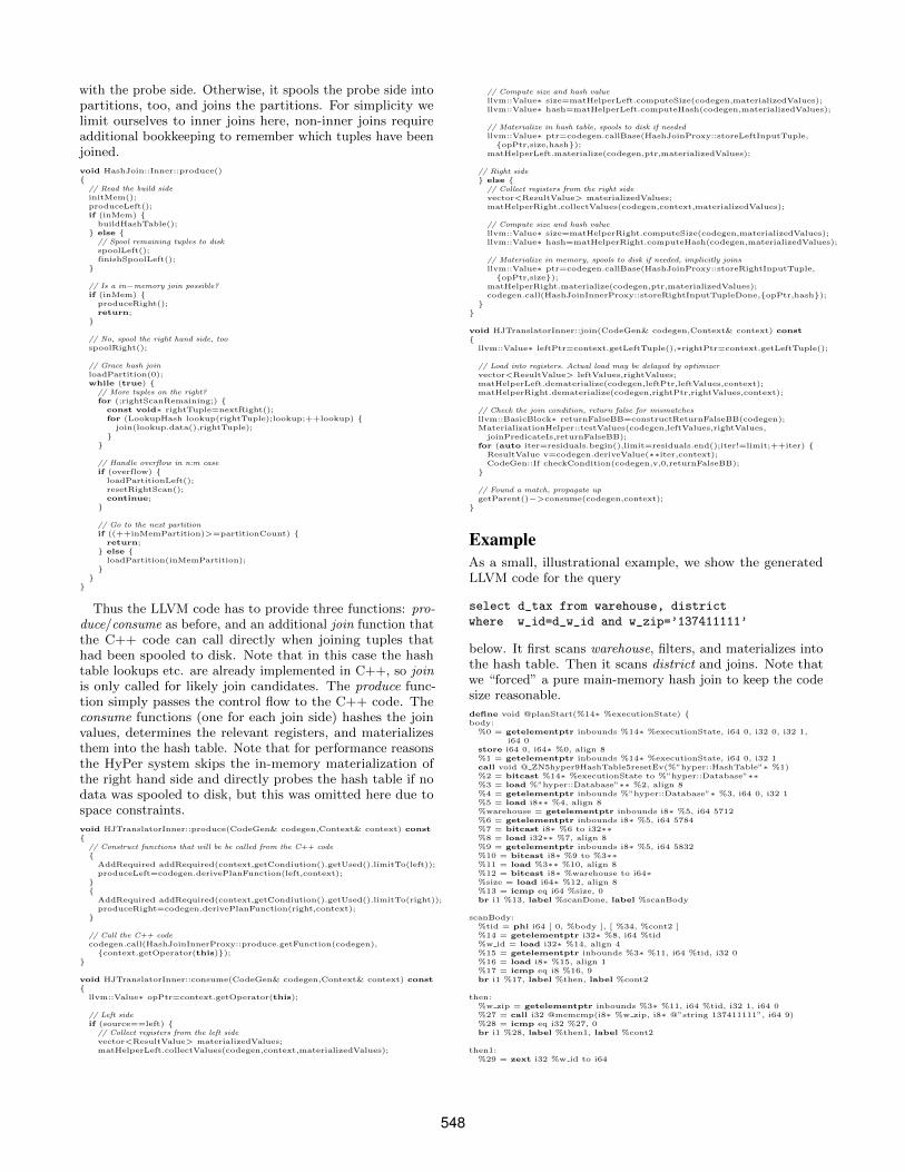
ExampleAs a small, illustrational example, we show the generatedLLVM code for the query

select d_tax from warehouse, district

where w_id=d_w_id and w_zip=’137411111’

below. It first scans warehouse, filters, and materializes intothe hash table. Then it scans district and joins. Note thatwe “forced” a pure main-memory hash join to keep the codesize reasonable.

define void @planStart(%14∗ %executionState) {body:

%0 = getelementptr inbounds %14∗ %executionState, i64 0, i32 0, i32 1,i64 0

store i64 0, i64∗ %0, align 8%1 = getelementptr inbounds %14∗ %executionState, i64 0, i32 1call void @ ZN5hyper9HashTable5resetEv(%”hyper::HashTable”∗ %1)%2 = bitcast %14∗ %executionState to %”hyper::Database”∗∗%3 = load %”hyper::Database”∗∗ %2, align 8%4 = getelementptr inbounds %”hyper::Database”∗ %3, i64 0, i32 1%5 = load i8∗∗ %4, align 8%warehouse = getelementptr inbounds i8∗ %5, i64 5712%6 = getelementptr inbounds i8∗ %5, i64 5784%7 = bitcast i8∗ %6 to i32∗∗%8 = load i32∗∗ %7, align 8%9 = getelementptr inbounds i8∗ %5, i64 5832%10 = bitcast i8∗ %9 to %3∗∗%11 = load %3∗∗ %10, align 8%12 = bitcast i8∗ %warehouse to i64∗%size = load i64∗ %12, align 8%13 = icmp eq i64 %size, 0br i1 %13, label %scanDone, label %scanBody

scanBody:%tid = phi i64 [ 0, %body ], [ %34, %cont2 ]%14 = getelementptr i32∗ %8, i64 %tid%w id = load i32∗ %14, align 4%15 = getelementptr inbounds %3∗ %11, i64 %tid, i32 0%16 = load i8∗ %15, align 1%17 = icmp eq i8 %16, 9br i1 %17, label %then, label %cont2

then:%w zip = getelementptr inbounds %3∗ %11, i64 %tid, i32 1, i64 0%27 = call i32 @memcmp(i8∗ %w zip, i8∗ @”string 137411111”, i64 9)%28 = icmp eq i32 %27, 0br i1 %28, label %then1, label %cont2

then1:%29 = zext i32 %w id to i64

548

%30 = call i64 @llvm.x86.sse42.crc64.64(i64 0, i64 %29)%31 = shl i64 %30, 32%32 = call i8∗ @ ZN5hyper9HashTable15storeInputTupleEmj(%”hyper::

HashTable”∗ %1, i64 %31, i32 4)%33 = bitcast i8∗ %32 to i32∗store i32 %w id, i32∗ %33, align 1br label %cont2

cont2:%34 = add i64 %tid, 1%35 = icmp eq i64 %34, %sizebr i1 %35, label %cont2.scanDone crit edge, label %scanBody

cont2.scanDone crit edge:%.pre = load %”hyper::Database”∗∗ %2, align 8%.phi.trans.insert = getelementptr inbounds %”hyper::Database”∗ %.pre,

i64 0, i32 1%.pre11 = load i8∗∗ %.phi.trans.insert, align 8br label %scanDone

scanDone:%18 = phi i8∗ [ %.pre11, %cont2.scanDone crit edge ], [ %5, %body ]%district = getelementptr inbounds i8∗ %18, i64 1512%19 = getelementptr inbounds i8∗ %18, i64 1592%20 = bitcast i8∗ %19 to i32∗∗%21 = load i32∗∗ %20, align 8%22 = getelementptr inbounds i8∗ %18, i64 1648%23 = bitcast i8∗ %22 to i64∗∗%24 = load i64∗∗ %23, align 8%25 = bitcast i8∗ %district to i64∗%size8 = load i64∗ %25, align 8%26 = icmp eq i64 %size8, 0br i1 %26, label %scanDone6, label %scanBody5

scanBody5:%tid9 = phi i64 [ 0, %scanDone ], [ %58, %loopDone ]%36 = getelementptr i32∗ %21, i64 %tid9%d w id = load i32∗ %36, align 4%37 = getelementptr i64∗ %24, i64 %tid9%d tax = load i64∗ %37, align 8%38 = zext i32 %d w id to i64%39 = call i64 @llvm.x86.sse42.crc64.64(i64 0, i64 %38)%40 = shl i64 %39, 32%41 = getelementptr inbounds %14∗ %executionState, i64 0, i32 1, i32 0%42 = load %”hyper::HashTable::Entry”∗∗∗ %41, align 8%43 = getelementptr inbounds %14∗ %executionState, i64 0, i32 1, i32 2%44 = load i64∗ %43, align 8%45 = lshr i64 %40, %44%46 = getelementptr %”hyper::HashTable::Entry”∗∗ %42, i64 %45%47 = load %”hyper::HashTable::Entry”∗∗ %46, align 8%48 = icmp eq %”hyper::HashTable::Entry”∗ %47, nullbr i1 %48, label %loopDone, label %loop

loopStep:%49 = getelementptr inbounds %”hyper::HashTable::Entry”∗ %iter, i64 0,

i32 1%50 = load %”hyper::HashTable::Entry”∗∗ %49, align 8%51 = icmp eq %”hyper::HashTable::Entry”∗ %50, nullbr i1 %51, label %loopDone, label %loop

loop:%iter = phi %”hyper::HashTable::Entry”∗ [ %47, %scanBody5 ], [ %50, %

loopStep ]%52 = getelementptr inbounds %”hyper::HashTable::Entry”∗ %iter, i64 1%53 = bitcast %”hyper::HashTable::Entry”∗ %52 to i32∗%54 = load i32∗ %53, align 4%55 = icmp eq i32 %54, %d w idbr i1 %55, label %then10, label %loopStep

then10:call void @ ZN6dbcore16RuntimeFunctions12printNumericEljj(i64 %d tax,

i32 4, i32 4)call void @ ZN6dbcore16RuntimeFunctions7printNlEv()br label %loopStep

loopDone:%58 = add i64 %tid9, 1%59 = icmp eq i64 %58, %size8br i1 %59, label %scanDone6, label %scanBody5

scanDone6:ret void}

B. MICROBENCHMARKSIn addition to the main experiments, we performed a num-

ber of micro-benchmarks to study the impact of differentquery processing schemes in more detail. We implementedseveral techniques and ran them within the HyPer system.This way, all approaches read exactly the same data fromexactly the same data structures, thus any runtime differ-ences stem purely from differences in data and control flowduring query processing. Besides the data-centric compi-lation scheme proposed in this paper, we implemented theclassical iterator model, both as interpreter (i.e., the standardevaluation scheme in most databases), and as compiled intoexecutable code. In addition, we implemented block-wisetuple processing [11], which roughly corresponds to the eval-

0

10

20

30

40

50

60

70

80

90

100

0 1 2 3

execution tim

e [m

s]

number of filtered columns

data-centric compilationiterator model - compiled

iterator model - interpretedblock processing - compiled

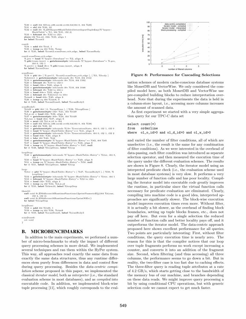
Figure 8: Performance for Cascading Selections

uation schemes of modern cache-conscious database systemslike MonetDB and VectorWise. We only considered the com-piled model here, as both MonetDB and VectorWise usepre-compiled building blocks to reduce interpretation over-head. Note that during the experiments the data is held ina column-store layout, i.e., accessing more columns increasesthe amount of scanned data.

As first experiment we started with a very simple aggrega-tion query for our TPC-C data set

select count(*)

from orderline

where ol_o_id>0 and ol_d_id>0 and ol_w_id>0

and varied the number of filter conditions, all of which areunselective (i.e., the result is the same for any combinationof filter conditions). As we were interested in the overhead ofdata-passing, each filter condition was introduced as separateselection operator, and then measured the execution time ofthe query under the different evaluation schemes. The resultsare shown in Figure 8. Clearly, the iterator model using aninterpreted predicate check (i.e., the evaluation scheme usedin most database systems) is very slow. It performs a verylarge number of function calls and has poor locality. Compil-ing the iterator model into executable code greatly improvesthe runtime, in particular since the virtual function callsnecessary for predicate evaluation are eliminated. Clearly,compiling into machine code is a good idea, interpreted ap-proaches are significantly slower. The block-wise executionmodel improves execution times even more. Without filter,it is actually a bit slower, as the overhead of finding blockboundaries, setting up tuple blocks frames, etc., does notpay off here. But even for a single selection the reducednumber of function calls and better locality pays off, and itoutperforms the iterator model. The data-centric approachproposed here shows excellent performance for all queries.Two points are particularly interesting: First, without filterconditions, the query execution time is nearly zero. Thereason for this is that the compiler notices that our loopover tuple fragments performs no work except increasing acounter, and converts it into an addition of the fragmentsize. Second, when filtering (and thus accessing) all threecolumns, the performance seems to go down a bit. But inreality, the two-filter case is too fast due to caching effects.The three-filter query is reading tuple attributes at a rateof 4.2 GB/s, which starts getting close to the bandwidth ofthe memory bus of our machine, and branches dependingon these data reads. We might improve query processing abit by using conditional CPU operations, but with genericselection code we cannot expect to get much faster.

549

0

10

20

30

40

50

60

1 2 3

execution tim

e [m

s]

number of aggregated columns

data-centric compilationiterator model - compiled

iterator model - interpretedblock processing - compiled

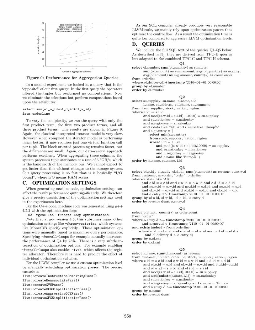
Figure 9: Performance for Aggregation Queries

In a second experiment we looked at a query that is the“opposite” of our first query: In the first query the operatorsfiltered the tuples but performed no computations. Nowwe eliminate the selections but perform computations basedupon the attributes:

select sum(ol_o_id*ol_d_id*ol_w_id)

from orderline

To vary the complexity, we ran the query with only thefirst product term, the first two product terms, and allthree product terms. The results are shown in Figure 9.Again, the classical interpreted iterator model is very slow.However when compiled the iterator model is performingmuch better, it now requires just one virtual function callper tuple. The block-oriented processing remains faster, butthe differences are small. Again, our data-centric approachperforms excellent. When aggregating three columns, thesystem processes tuple attributes at a rate of 6.5GB/s, whichis the bandwidth of the memory bus. We cannot expect toget faster than this without changes to the storage system.Our query processing is so fast that is is basically “I/Obound”, where I/O means RAM access.

C. OPTIMIZATION SETTINGSWhen generating machine code, optimization settings can

affect the result performance quite significantly. We thereforegive a precise description of the optimization settings usedin the experiments here.

For the C++ code, machine code was generated using g++4.5.2 with the optimization flags-O3 -fgcse-las -funsafe-loop-optimizations.Note that at gcc version 4.5, this subsumes many other

optimization settings like -ftree-vectorize, which systemslike MonetDB specify explicitly. These optimization op-tions were manually tuned to maximize query performance.Specifying -funroll-loops for example actually decreasesthe performance of Q4 by 23%. There is a very subtle in-teraction of optimization options. For example enabling-funroll-loops also enables -fweb, which affects the regis-ter allocator. Therefore it is hard to predict the effect ofindividual optimization switches.

For the LLVM compiler we use a custom optimization levelby manually scheduling optimization passes. The precisecascade isllvm::createInstructionCombiningPass()

llvm::createReassociatePass()

llvm::createGVNPass()

llvm::createCFGSimplificationPass()

llvm::createAggressiveDCEPass()

llvm::createCFGSimplificationPass()

As our SQL compiler already produces very reasonableLLVM code, we mainly rely upon optimization passes thatoptimize the control flow. As a result the optimization time isquite low compared to aggressive LLVM optimization levels.

D. QUERIESWe include the full SQL text of the queries Q1-Q5 below.

As described in [5], they are derived from TPC-H queriesbut adapted to the combined TPC-C and TPC-H schema.

Q1select ol number, sum(ol quantity) as sum qty,

sum(ol amount) as sum amount, avg(ol quantity) as avg qty,avg(ol amount) as avg amount, count(∗) as count order

from orderlinewhere ol delivery d>timestamp ’2010−01−01 00:00:00’group by ol numberorder by ol number

Q2select su suppkey, su name, n name, i id,

i name, su address, su phone, su commentfrom item, supplier, stock, nation, regionwhere i id = s i id

and mod((s w id ∗ s i id), 10000) = su suppkeyand su nationkey = n nationkeyand n regionkey = r regionkeyand i data like ’%b’ and r name like ’Europ%’and s quantity = (

select min(s quantity)from stock, supplier, nation, regionwhere i id = s i id

and mod((s w id ∗ s i id),10000) = su suppkeyand su nationkey = n nationkeyand n regionkey = r regionkeyand r name like ’Europ%’ )

order by n name, su name, i id

Q3select ol o id , ol w id , ol d id , sum(ol amount) as revenue, o entry dfrom customer, neworder, ”order”, orderlinewhere c state like ’A%’

and c id = o c id and c w id = o w id and c d id = o d idand no w id = o w id and no d id = o d id and no o id = o idand ol w id = o w id and ol d id = o d id and ol o id = o idand o entry d > timestamp ’2010−01−01 00:00:00’

group by ol o id, ol w id, ol d id , o entry dorder by revenue desc, o entry d

Q4select o ol cnt , count(∗) as order countfrom ”order”where o entry d >= timestamp ’2010−01−01 00:00:00’

and o entry d < timestamp ’2110−01−01 00:00:00’and exists (select ∗ from orderline

where o id = ol o id and o w id = ol w id and o d id = ol d idand ol delivery d > o entry d)

group by o ol cntorder by o ol cnt

Q5select n name, sum(ol amount) as revenuefrom customer, ”order”, orderline, stock, supplier , nation, regionwhere c id = o c id and c w id = o w id and c d id = o d id

and ol o id = o id and ol w id = o w id and ol d id=o d idand ol w id = s w id and ol i id = s i idand mod((s w id ∗ s i id),10000) = su suppkeyand ascii(substr(c state ,1,1)) = su nationkeyand su nationkey = n nationkeyand n regionkey = r regionkey and r name = ’Europa’and o entry d >= timestamp ’2010−01−01 00:00:00’

group by n nameorder by revenue desc

550