efficient parallel set-similarity joins using mapreduce rares vernica, michael j. carey, chen li...

Efficient Parallel Set-Similarity Joins Using MapReduce

Rares Vernica, Michael J. Carey, Chen Li

Speaker : Razvan Belet

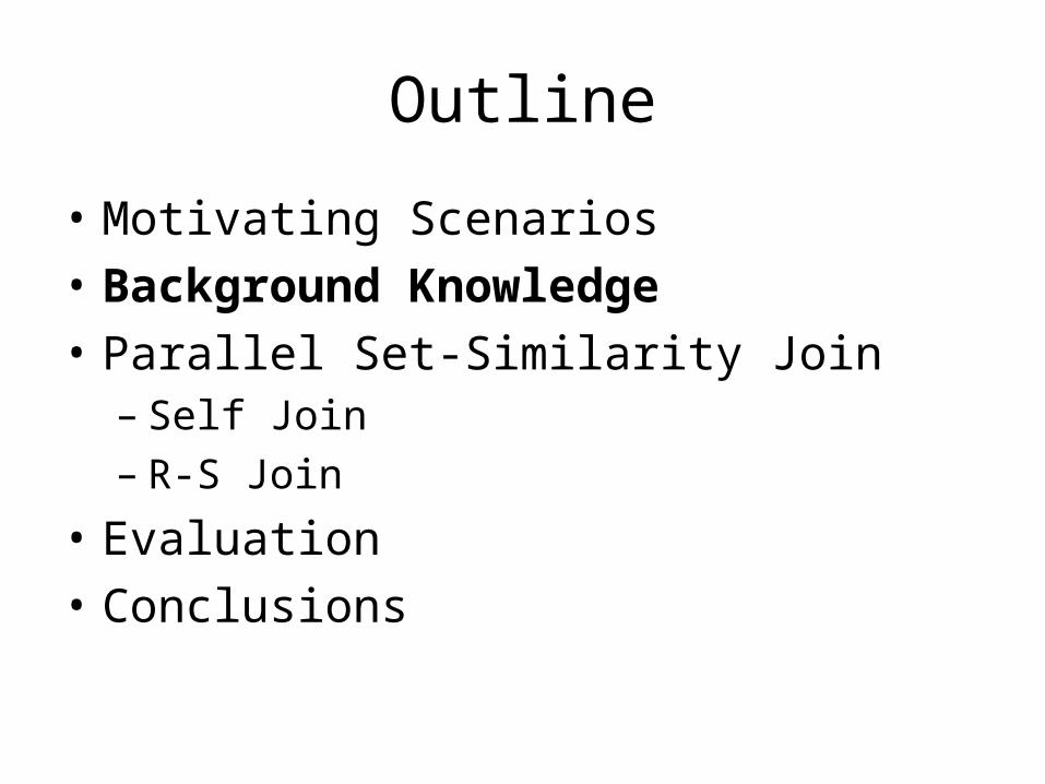
Outline

• Motivating Scenarios

• Background Knowledge

• Parallel Set-Similarity Join– Self Join– R-S Join

• Evaluation

• Conclusions

• Strengths & Weaknesses

Scenario: Detecting Plagiarism

• Before publishing a Journal, editors have to make sure there is no plagiarized paper among the hundreds of papers to be included in the Journal

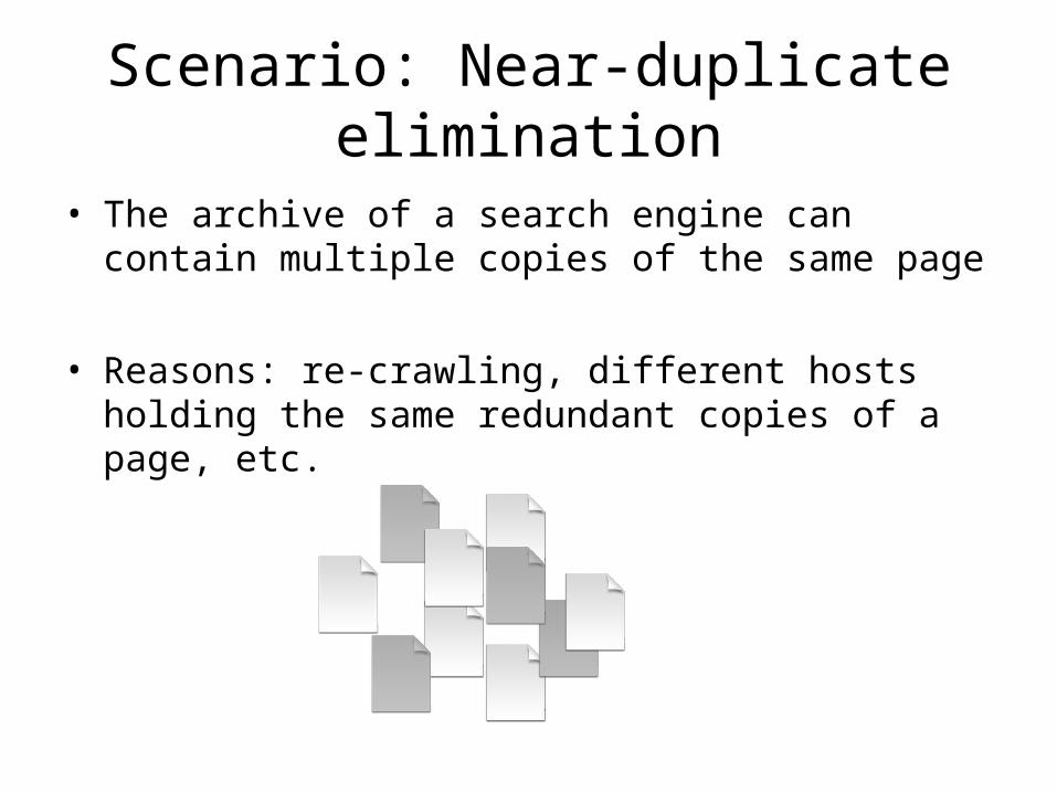
Scenario: Near-duplicate elimination

• The archive of a search engine can contain multiple copies of the same page

• Reasons: re-crawling, different hosts holding the same redundant copies of a page, etc.

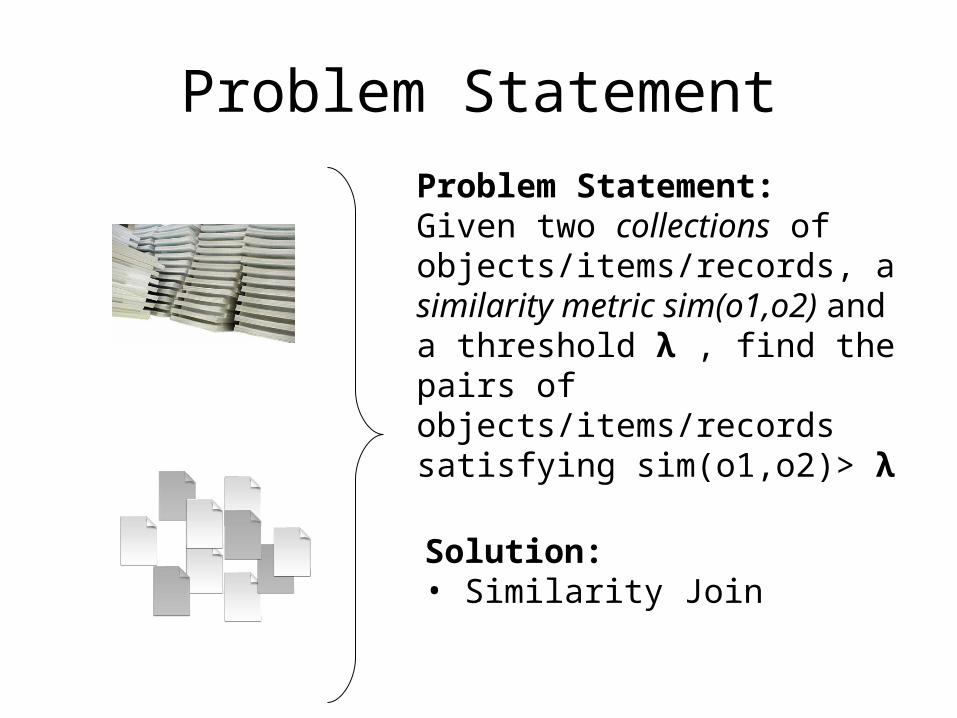
Problem Statement

Problem Statement: Given two collections of objects/items/records, a similarity metric sim(o1,o2) and a threshold λ , find the pairs of objects/items/records satisfying sim(o1,o2)> λ

Solution: • Similarity Join

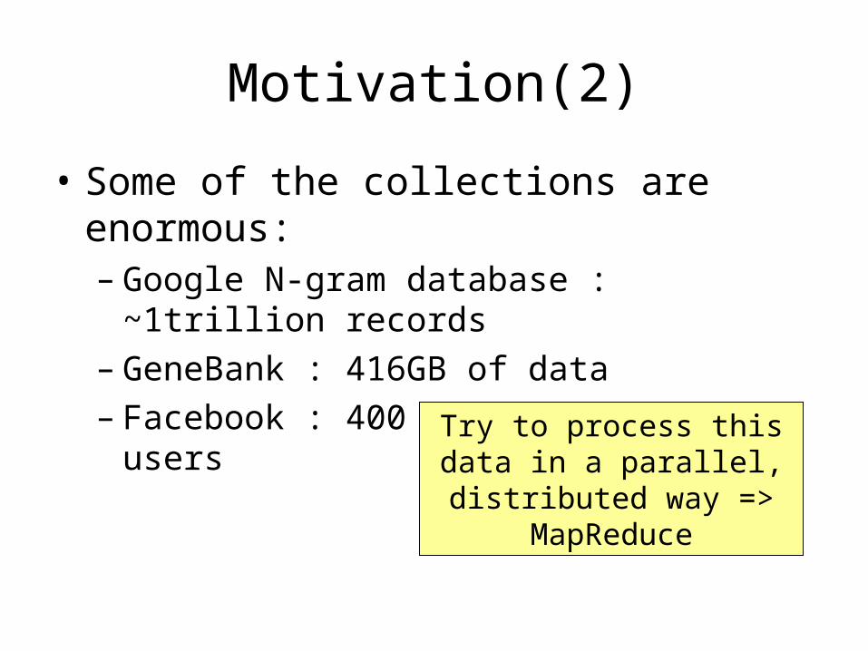
Motivation(2)

• Some of the collections are enormous:– Google N-gram database : ~1trillion records– GeneBank : 416GB of data– Facebook : 400 million active users

Try to process this data in a parallel, distributed way

=> MapReduce

Outline




• Evaluation

• Conclusions

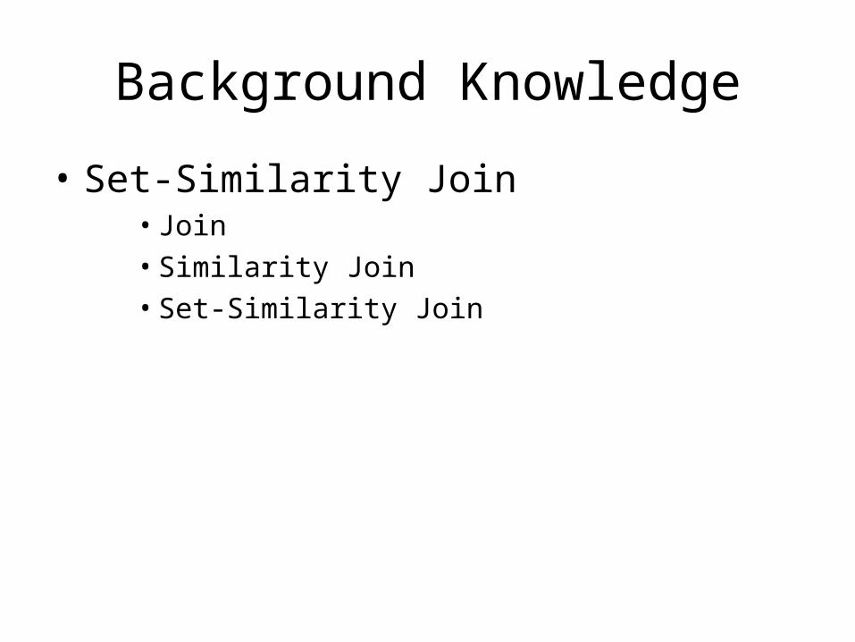
Background Knowledge

• Set-Similarity Join• Join• Similarity Join• Set-Similarity Join

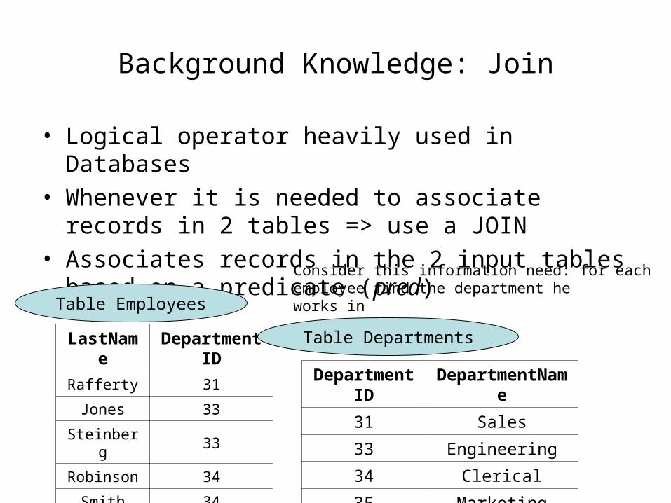
Background Knowledge: Join

• Logical operator heavily used in Databases• Whenever it is needed to associate records in 2 tables

=> use a JOIN• Associates records in the 2 input tables based on a

predicate (pred)

LastName DepartmentID

Rafferty 31

Jones 33

Steinberg 33

Robinson 34

Smith 34

John NULL

DepartmentID DepartmentName

31 Sales

33 Engineering

34 Clerical

35 Marketing

Table Employees

Table Departments

Consider this information need: for each employee find the department he works in

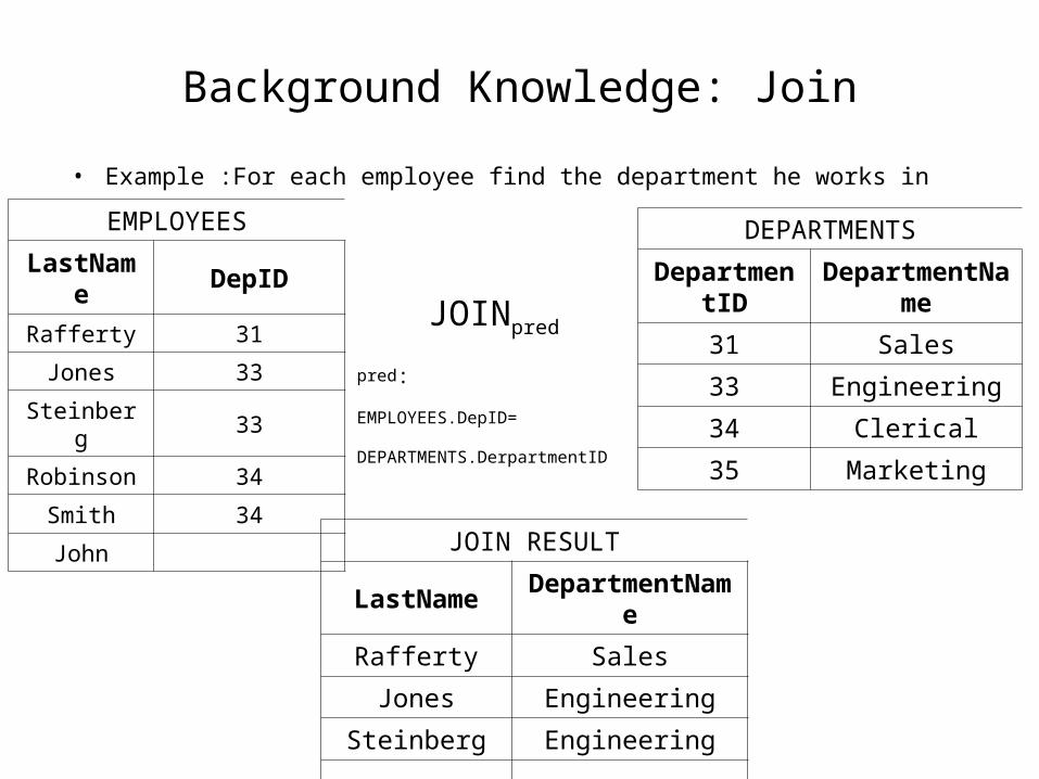
Background Knowledge: Join

EMPLOYEES

LastName DepID

Rafferty 31

Jones 33

Steinberg 33

Robinson 34

Smith 34

John NULL

DEPARTMENTS

DepartmentID

DepartmentName

31 Sales

33 Engineering

34 Clerical

35 Marketing

• Example :For each employee find the department he works in

JOINpred

pred:

EMPLOYEES.DepID=

DEPARTMENTS.DerpartmentID

JOIN RESULT

LastName DepartmentName

Rafferty Sales

Jones Engineering

Steinberg Engineering

… …

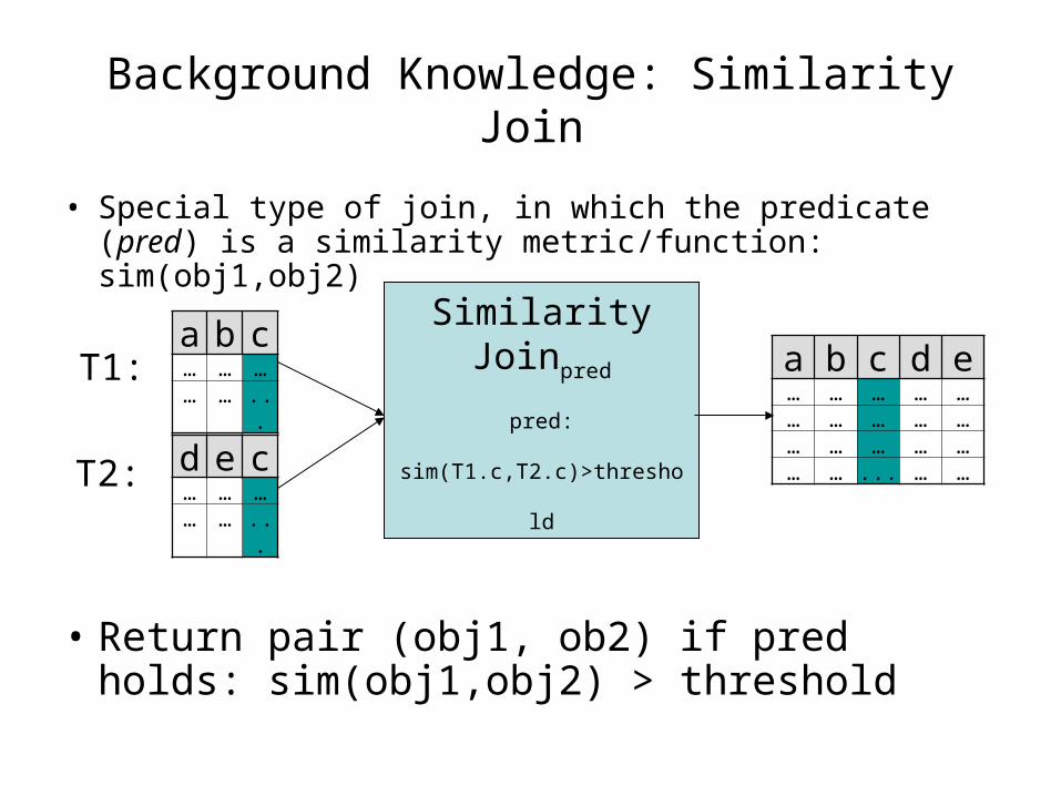
Background Knowledge: Similarity Join

• Special type of join, in which the predicate (pred) is a similarity metric/function: sim(obj1,obj2)

• Return pair (obj1, ob2) if pred holds: sim(obj1,obj2) > threshold

Similarity Joinpred

pred: sim(T1.c,T2.c)>threshold

a b c… … …… … ...

d e c… … …… … ...

T1:

T2:

a b c d e… … … … …… … … … …… … … … …… … ... … …

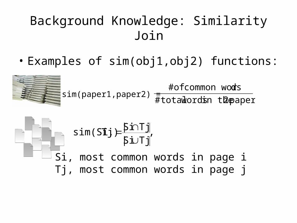
Background Knowledge: Similarity Join

• Examples of sim(obj1,obj2) functions:

sim(paper1,paper2) =papers 2 in the wordstotal#

dscommon wor of#

|TjSi||TjSi|Tj)sim(Si,

Si, most common words in page iTj, most common words in page j

,

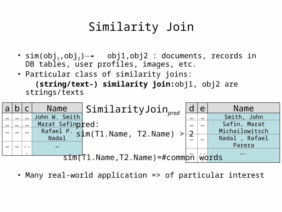
Similarity Join

• sim(obj1,obj2) obj1,obj2 : documents, records in DB tables, user profiles, images, etc.

• Particular class of similarity joins: (string/text-) similarity join:obj1, obj2 are strings/texts

• Many real-world application => of particular interest

a b c Name… … … John W. Smith… … … Marat Safin… … … Rafael P. Nadal… … ... …

d e Name… … Smith, John… … Safin, Marat Michailowitsch… … Nadal , Rafael Parera… ... ….

SimilarityJoinpred

sim(T1.Name,T2.Name)=#common words

pred: sim(T1.Name, T2.Name) > 2

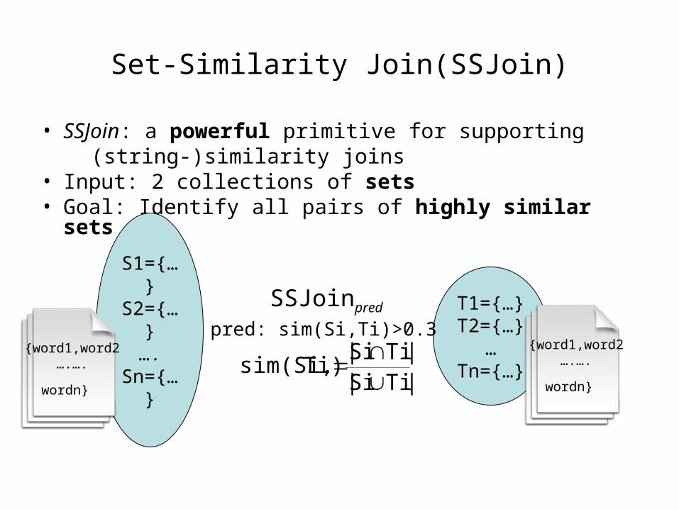
Set-Similarity Join(SSJoin)

• SSJoin: a powerful primitive for supporting (string-)similarity joins• Input: 2 collections of sets• Goal: Identify all pairs of highly similar sets

S1={…}

S2={…}

….Sn={…

}

T1={…}T2={…}

…Tn={…}

SSJoinpred

pred: sim(Si,Ti)>0.3{word1,word2

….….

wordn}

{word1,word2….….

wordn} |TiSi||TiSi|

Ti)sim(Si,

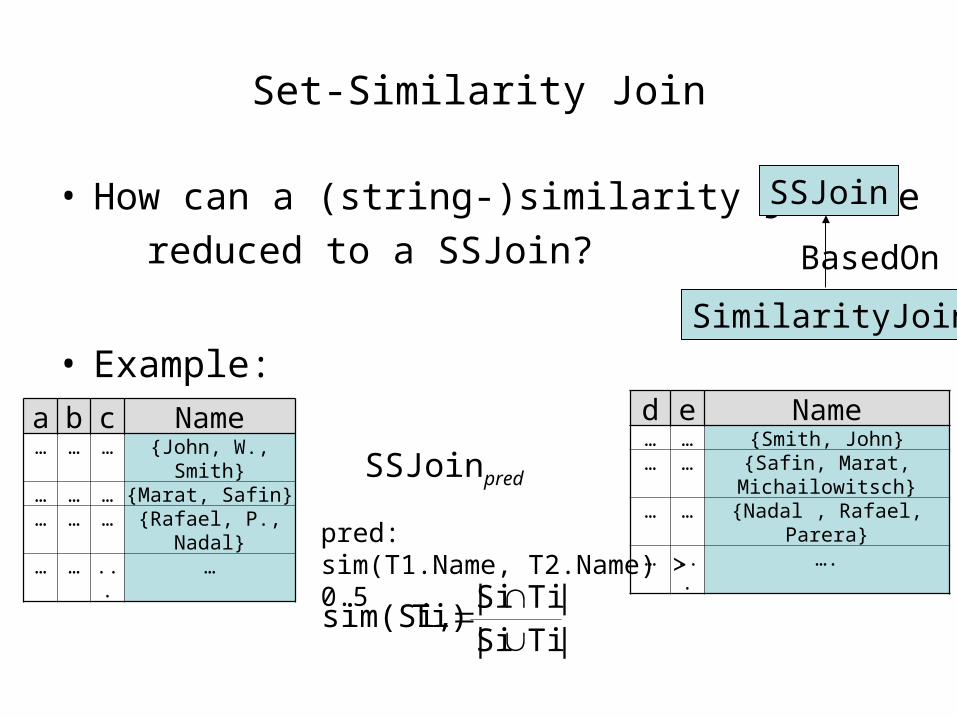
Set-Similarity Join

• How can a (string-)similarity join be

reduced to a SSJoin?

• Example:SimilarityJoin

SSJoin

BasedOn

a b c Name… … … {John, W., Smith}… … … {Marat, Safin}… … … {Rafael, P., Nadal}… … ... …

d e Name… … {Smith, John}… … {Safin, Marat,

Michailowitsch}… … {Nadal , Rafael, Parera}… ... ….pred:

sim(T1.Name, T2.Name) > 0.5

SSJoinpred

|TiSi||TiSi|

Ti)sim(Si,

Set-Similarity Join

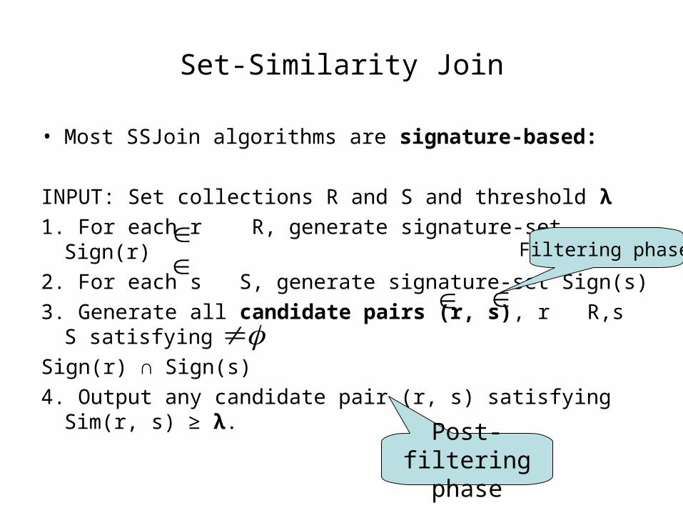
• Most SSJoin algorithms are signature-based:

INPUT: Set collections R and S and threshold λ

1. For each r R, generate signature-set Sign(r)

2. For each s S, generate signature-set Sign(s)

3. Generate all candidate pairs (r, s), r R,s S satisfying

Sign(r) ∩ Sign(s)

4. Output any candidate pair (r, s) satisfying Sim(r, s) ≥ λ.

Filtering phase

Post-filtering phase

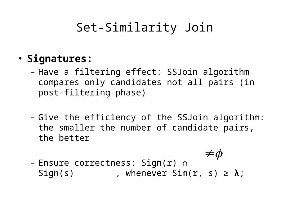
Set-Similarity Join

• Signatures: – Have a filtering effect: SSJoin algorithm compares

only candidates not all pairs (in post-filtering phase)

– Give the efficiency of the SSJoin algorithm: the smaller the number of candidate pairs, the better

– Ensure correctness: Sign(r) ∩ Sign(s) , whenever Sim(r, s) ≥ λ;

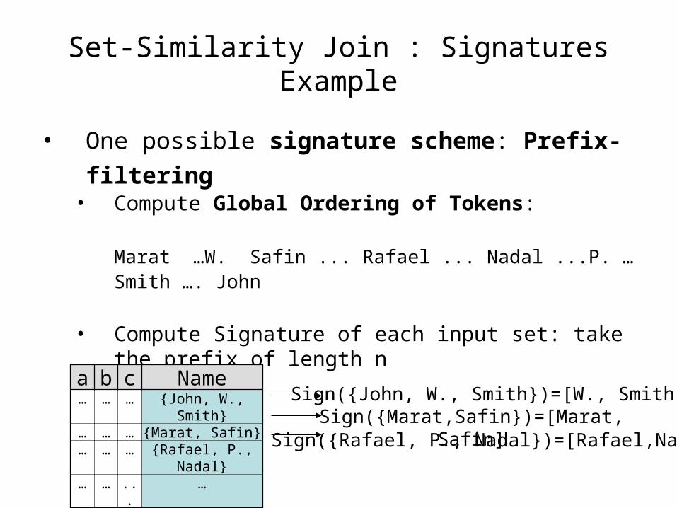
Set-Similarity Join : Signatures Example

• One possible signature scheme: Prefix-filtering • Compute Global Ordering of Tokens:

Marat …W. Safin ... Rafael ... Nadal ...P. … Smith …. John

• Compute Signature of each input set: take the prefix of length n

Sign({John, W., Smith})=[W., Smith]Sign({Marat,Safin})=[Marat, Safin]Sign({Rafael, P., Nadal})=[Rafael,Nadal]

a b c Name… … … {John, W., Smith}… … … {Marat, Safin}… … … {Rafael, P., Nadal}… … ... …

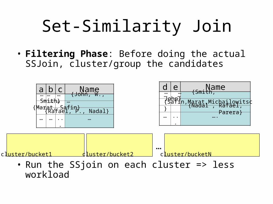
Set-Similarity Join

• Filtering Phase: Before doing the actual SSJoin, cluster/group the candidates

• Run the SSjoin on each cluster => less workload

…cluster/bucket1 cluster/bucket2 cluster/bucketN

d e Name

… ... ….

a b c Name

… … ... …

… … … {John, W., Smith} … … … {Marat, Safin}

{Rafael, P., Nadal}

… … {Smith, John}… … {Safin,Marat,Michailowitsc}

{Nadal , Rafael, Parera}

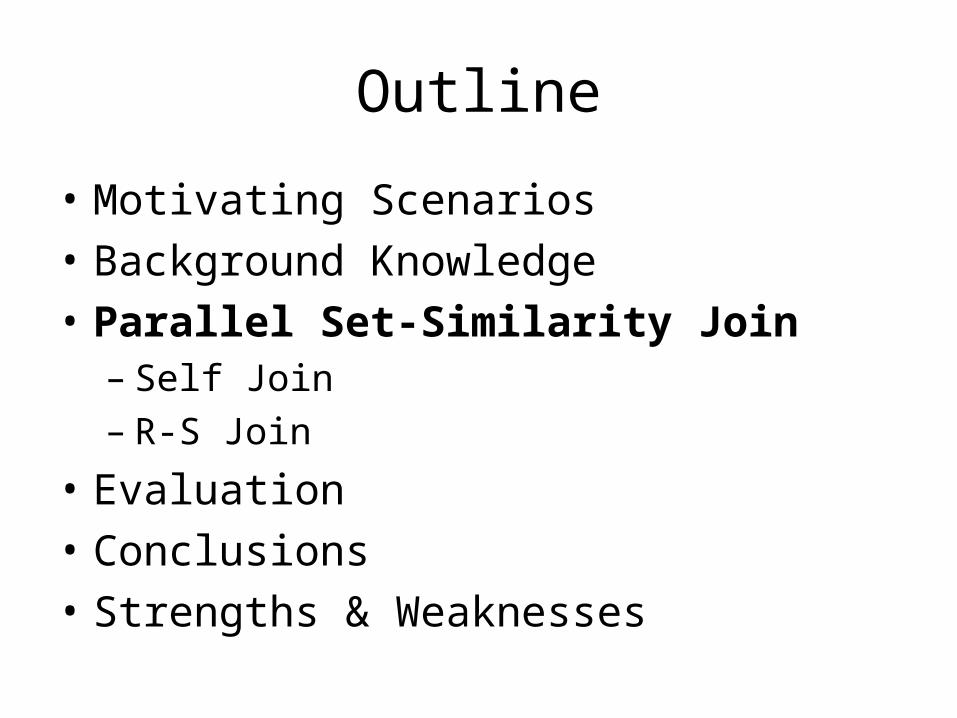
Outline




• Evaluation

• Conclusions


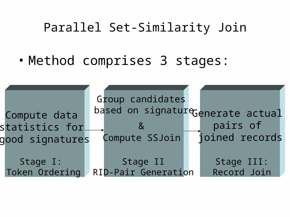
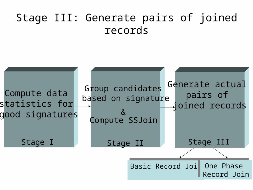
Parallel Set-Similarity Join

• Method comprises 3 stages:

Generate actual pairs of

joined records

Group candidates based on signature

Compute SSJoin&

Compute data statistics for

good signatures

Stage IIRID-Pair Generation

Stage I: Token Ordering

Stage III:Record Join

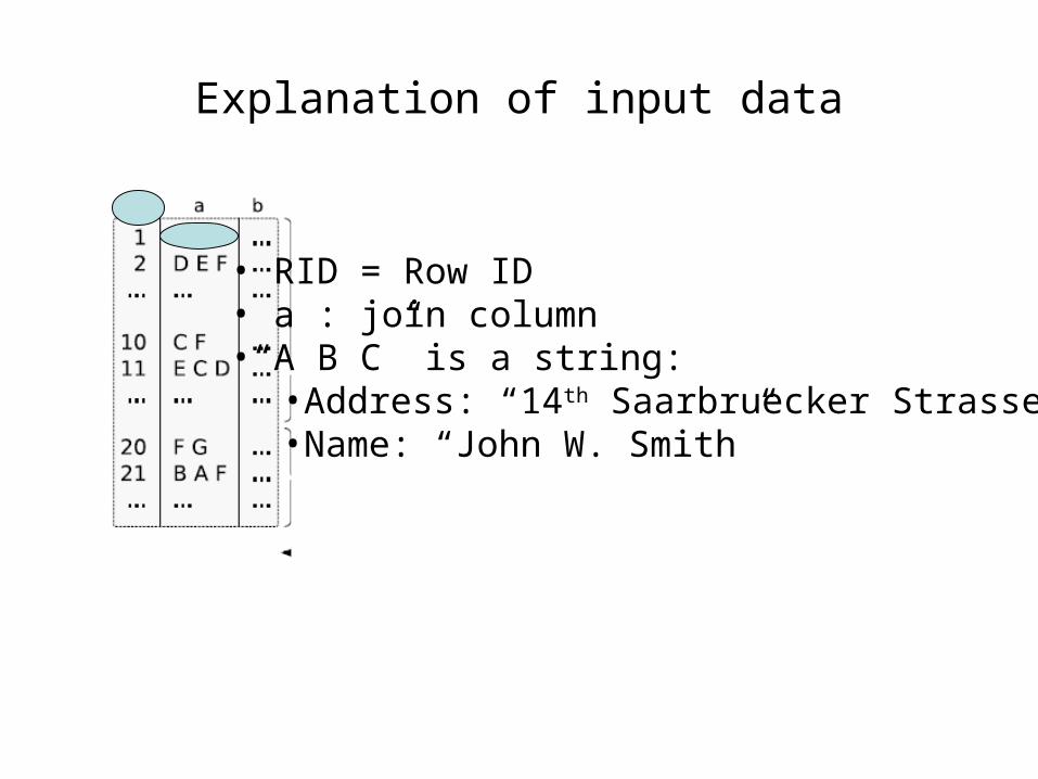
Explanation of input data

• RID = Row ID• a : join column •“A B C” is a string:

•Address: “14th Saarbruecker Strasse”•Name: “John W. Smith”

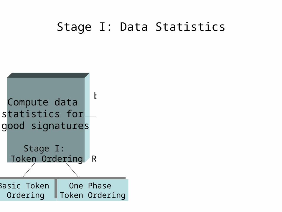
Stage I: Data Statistics


joined records


Compute SSJoin&


good signatures

Basic Token Ordering

Basic Token Ordering

One Phase Token Ordering

One Phase Token Ordering




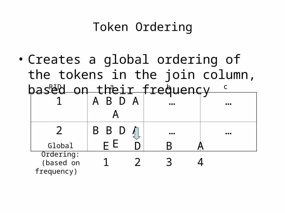
Token Ordering

• Creates a global ordering of the tokens in the join column, based on their frequency

1 A B D A A … …

2 B B D A E … …

RID a b c

Global Ordering:(based on

frequency)

E D B A

1 2 3 4

Basic Token Ordering(BTO)

• 2 MapReduce cycles:– 1st : computing token frequencies– 2nd: ordering the tokens by their frequencies

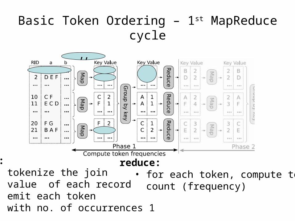
Basic Token Ordering – 1st MapReduce cycle

map:• tokenize the join value of each record• emit each token with no. of occurrences 1

, ,

reduce:• for each token, compute total count (frequency)

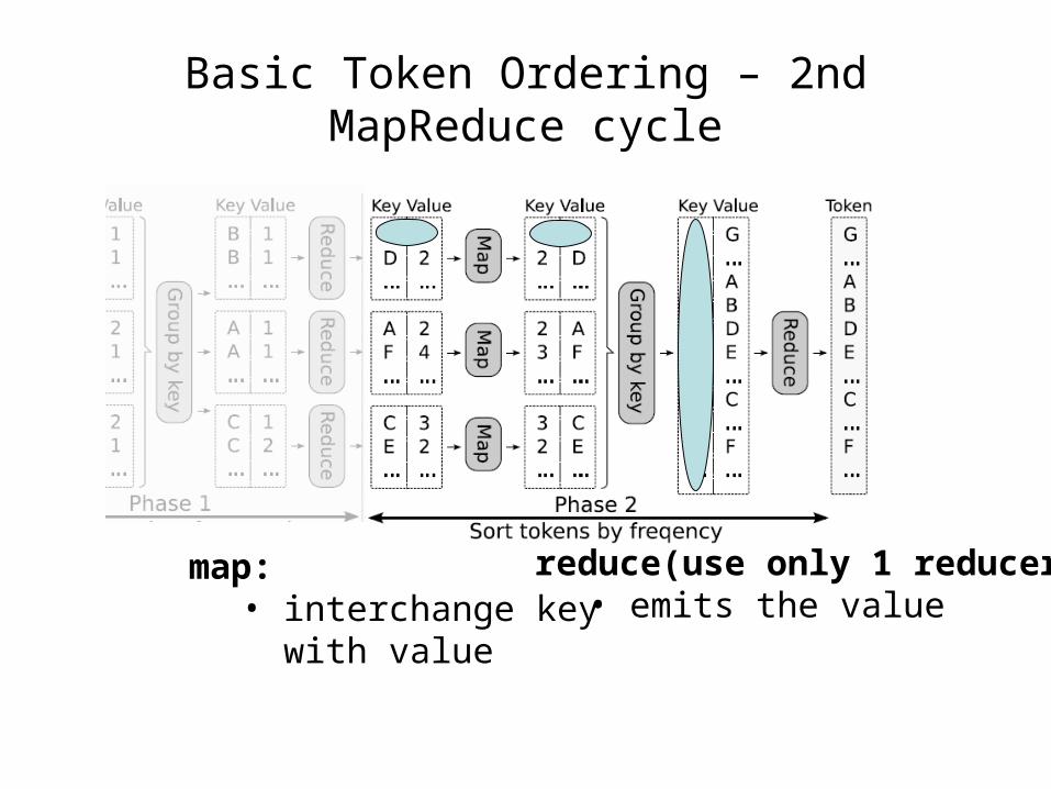
Basic Token Ordering – 2nd MapReduce cycle

map:• interchange key with value

reduce(use only 1 reducer):• emits the value

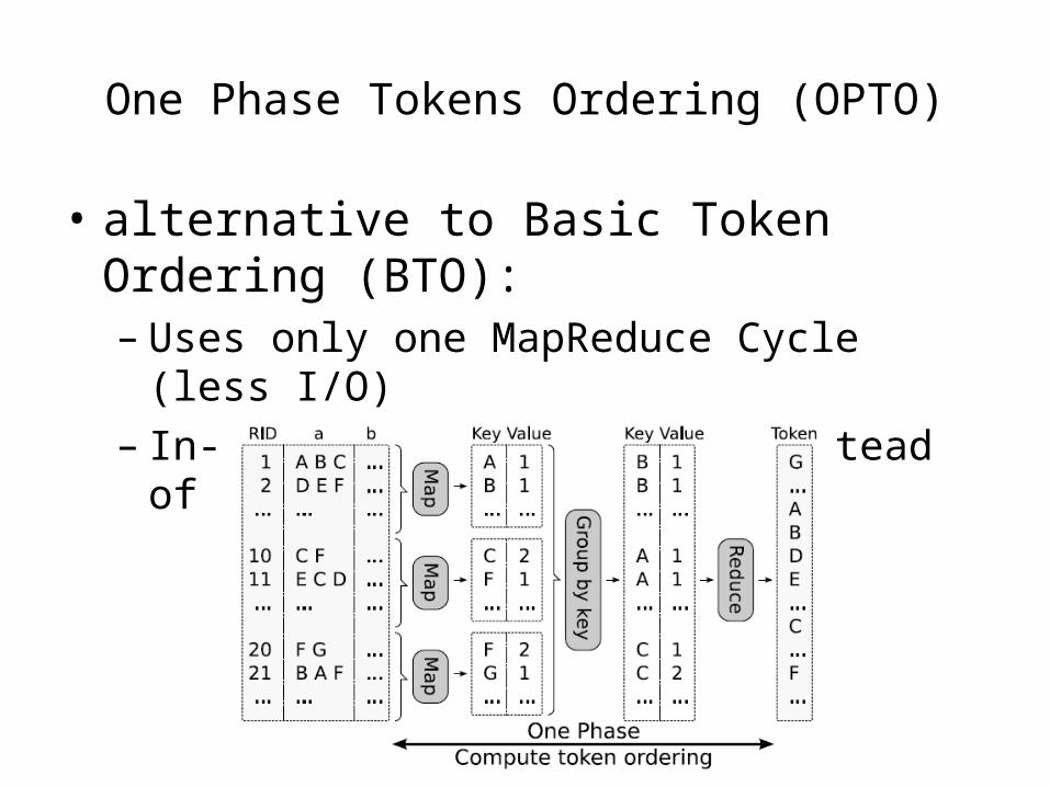
One Phase Tokens Ordering (OPTO)

• alternative to Basic Token Ordering (BTO):– Uses only one MapReduce Cycle (less I/O)– In-memory token sorting, instead of using a

reducer

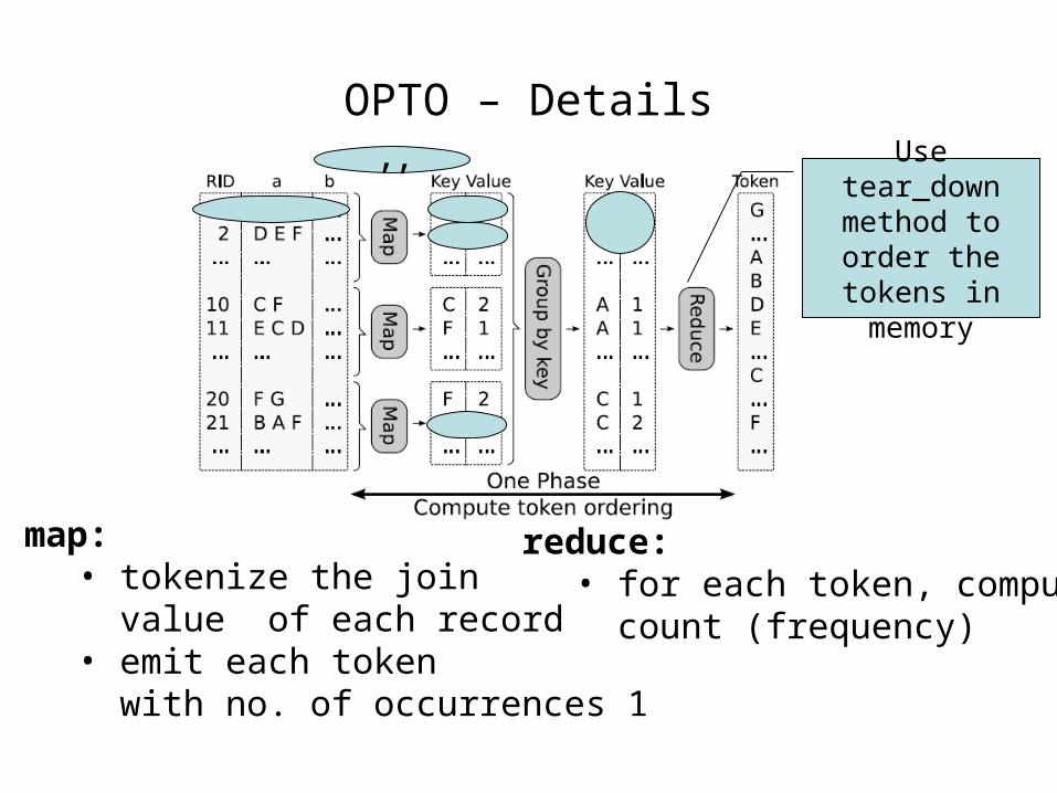
OPTO – Details

map:• tokenize the join value of each record• emit each token with no. of occurrences 1

, ,

reduce:• for each token, compute total count (frequency)

Use tear_down method to order

the tokens in memory

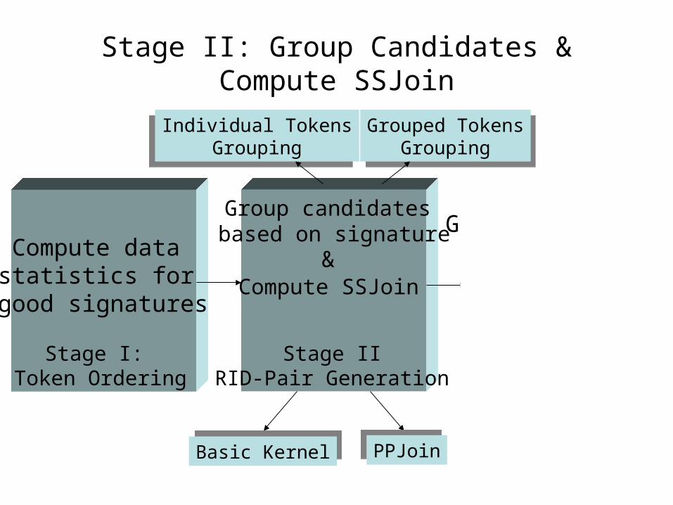
Stage II: Group Candidates & Compute SSJoin


joined records



Compute SSJoin&Compute data

statistics for good signatures



Individual TokensGrouping

Individual TokensGrouping

Grouped TokensGrouping

Grouped TokensGrouping

Basic KernelBasic Kernel PPJoinPPJoin

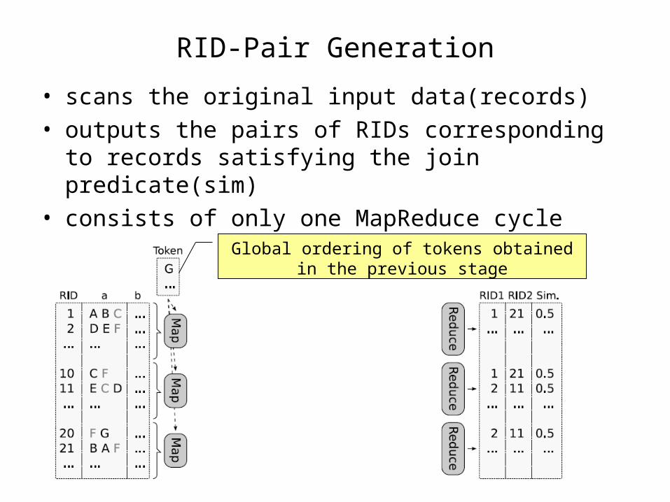
RID-Pair Generation

• scans the original input data(records) • outputs the pairs of RIDs corresponding to records

satisfying the join predicate(sim)• consists of only one MapReduce cycle

Global ordering of tokens obtained in the previous stage

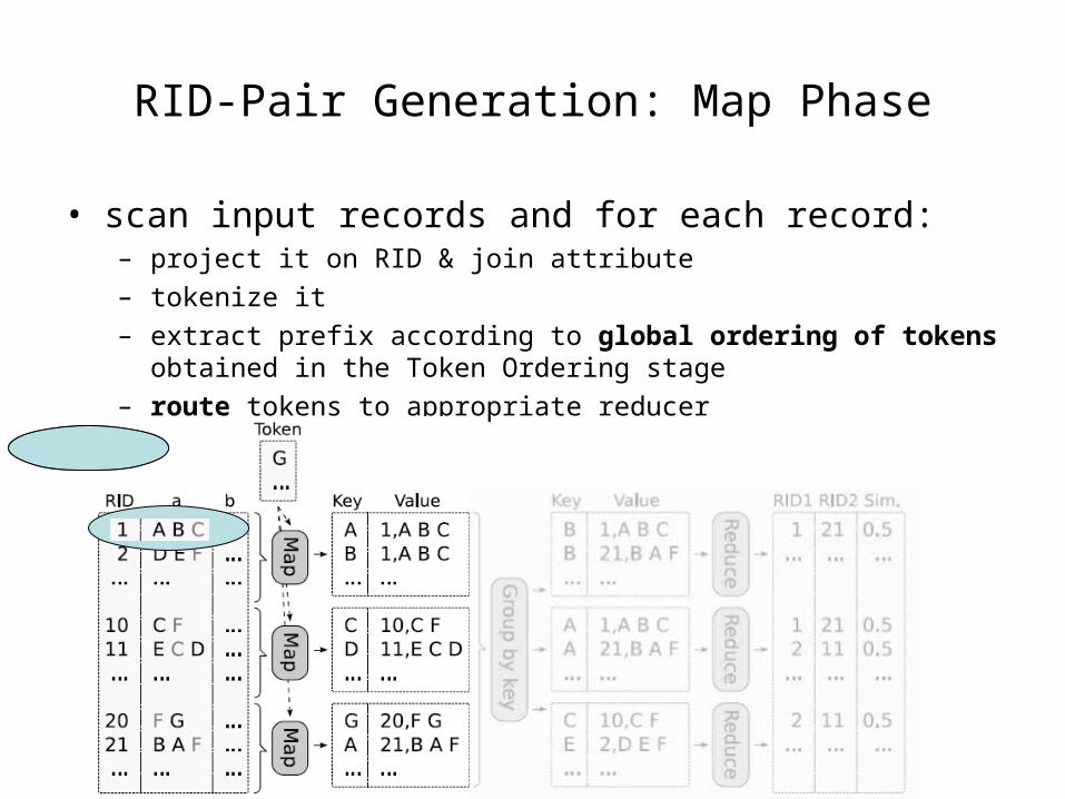
RID-Pair Generation: Map Phase

• scan input records and for each record:– project it on RID & join attribute

– tokenize it

– extract prefix according to global ordering of tokens obtained in the Token Ordering stage

– route tokens to appropriate reducer

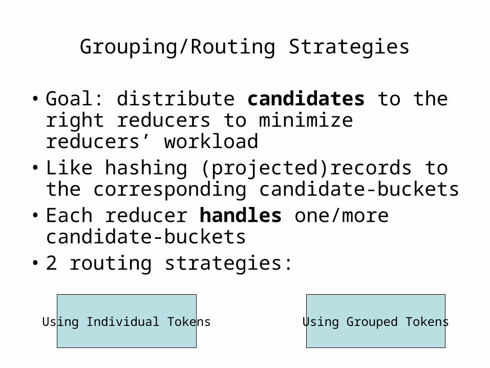
Grouping/Routing Strategies

• Goal: distribute candidates to the right reducers to minimize reducers’ workload

• Like hashing (projected)records to the corresponding candidate-buckets

• Each reducer handles one/more candidate-buckets

• 2 routing strategies:

Using Individual Tokens Using Grouped Tokens

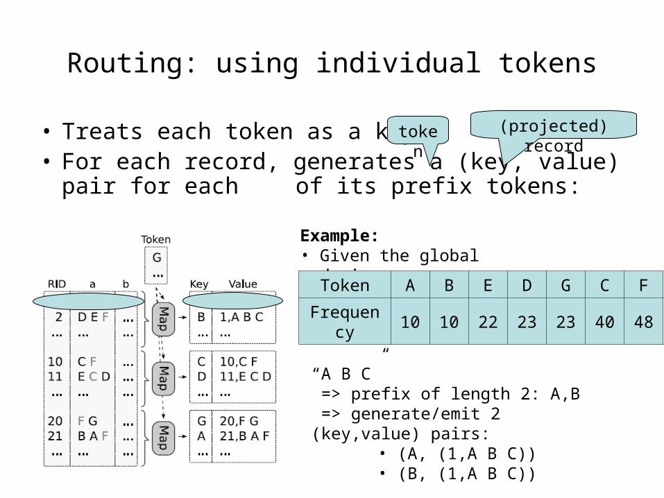
Routing: using individual tokens

• Treats each token as a key• For each record, generates a (key, value) pair

for each of its prefix tokens:

token (projected) record

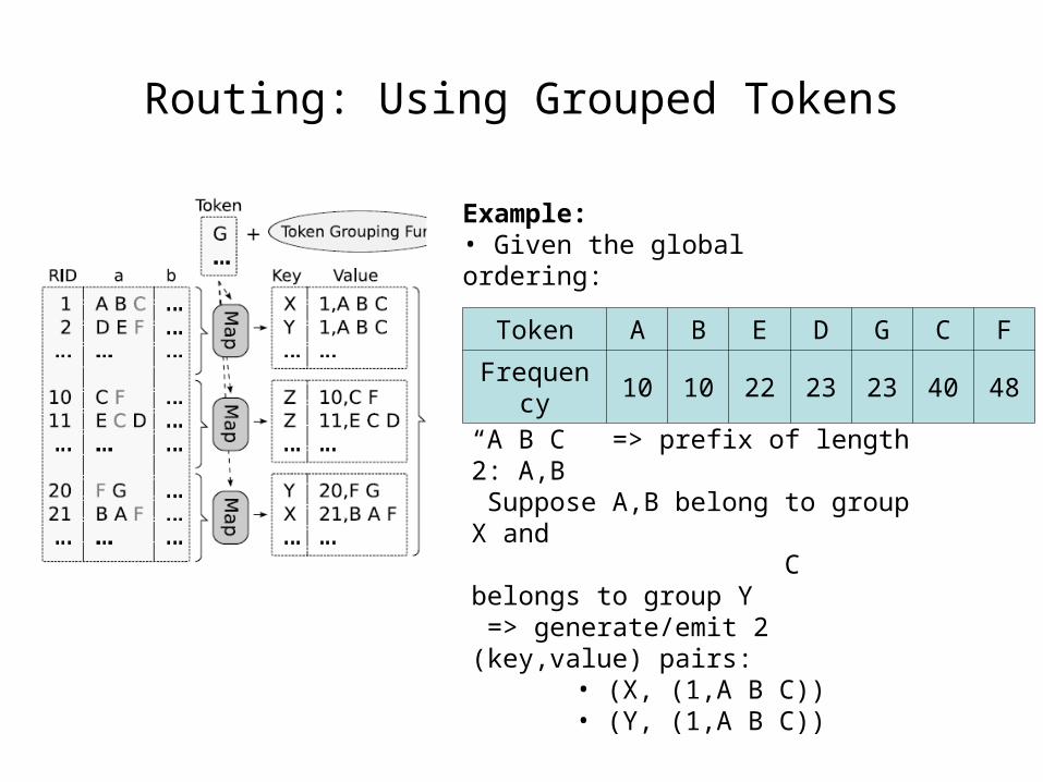
Example: • Given the global ordering:

Token A B E D G C F

Frequency 10 10 22 23 23 40 48

“A B C” => prefix of length 2: A,B => generate/emit 2 (key,value) pairs:

• (A, (1,A B C))• (B, (1,A B C))

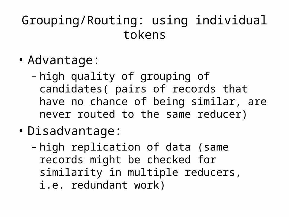
Grouping/Routing: using individual tokens

• Advantage: – high quality of grouping of candidates( pairs of

records that have no chance of being similar, are never routed to the same reducer)

• Disadvantage: – high replication of data (same records might

be checked for similarity in multiple reducers, i.e. redundant work)

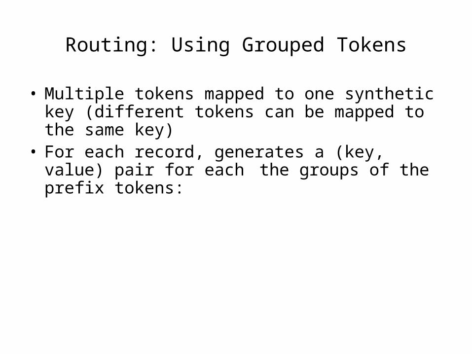
Routing: Using Grouped Tokens

• Multiple tokens mapped to one synthetic key (different tokens can be mapped to the same key)

• For each record, generates a (key, value) pair for each the groups of the prefix tokens:

Routing: Using Grouped Tokens

“A B C” => prefix of length 2: A,B Suppose A,B belong to group X and C belongs to group Y => generate/emit 2 (key,value) pairs:

• (X, (1,A B C))• (Y, (1,A B C))

Example: • Given the global ordering:

Token A B E D G C F

Frequency 10 10 22 23 23 40 48

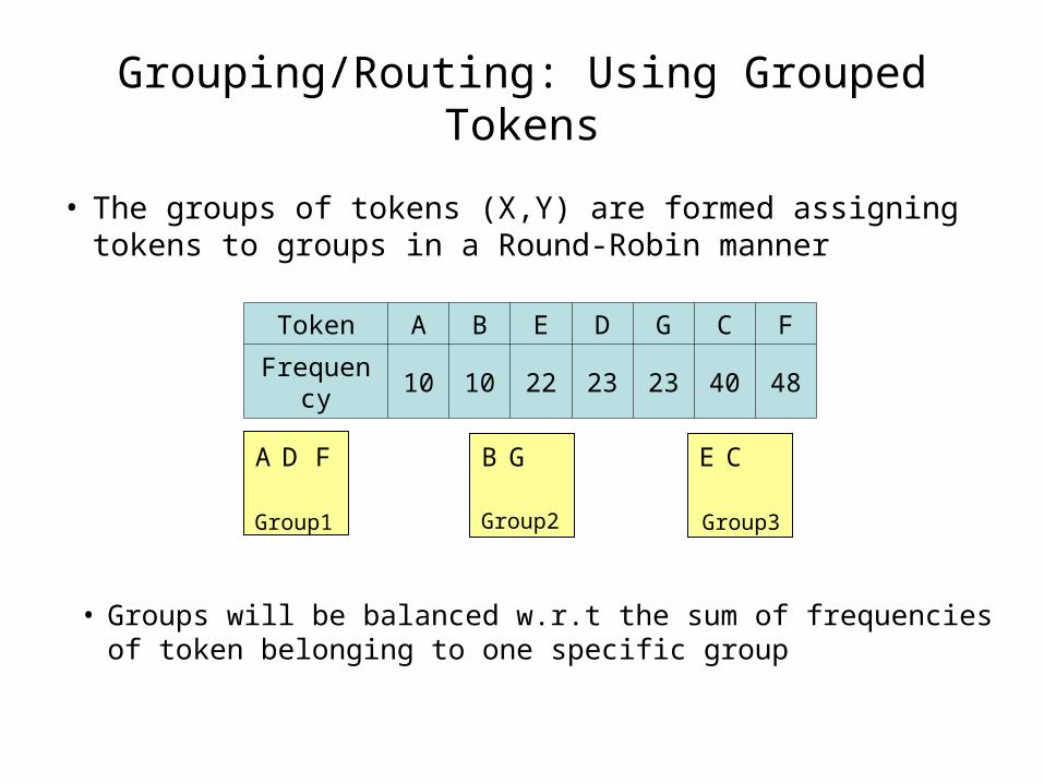
Grouping/Routing: Using Grouped Tokens

• The groups of tokens (X,Y) are formed assigning tokens to groups in a Round-Robin manner

Token A B E D G C F

Frequency 10 10 22 23 23 40 48

Group1 Group3Group2

A D F B EG C

• Groups will be balanced w.r.t the sum of frequencies of token belonging to one specific group

Grouping/Routing: Using Grouped Tokens

• Advantage: – Replication of data is not so pervasive

• Disadvantage:– Quality of grouping is not so high (records

having no chance of being similar are sent to the same reducer which checks their similarity)

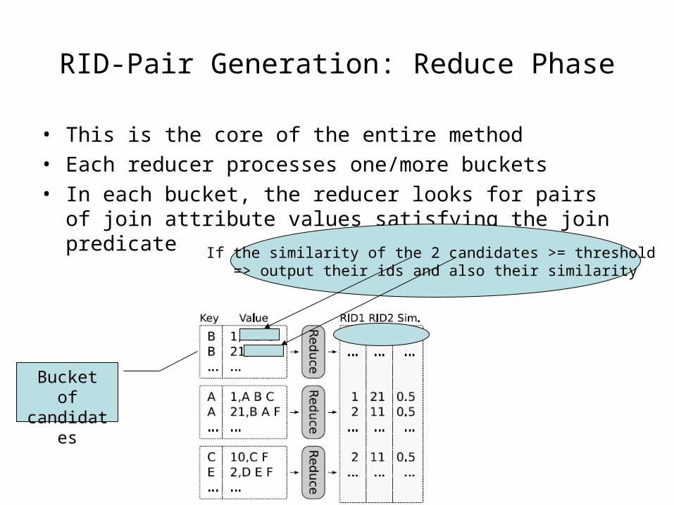
RID-Pair Generation: Reduce Phase

• This is the core of the entire method

• Each reducer processes one/more buckets

• In each bucket, the reducer looks for pairs of join attribute values satisfying the join predicate

Bucket of candidates

If the similarity of the 2 candidates >= threshold => output their ids and also their similarity

RID-Pair Generation: Reduce Phase

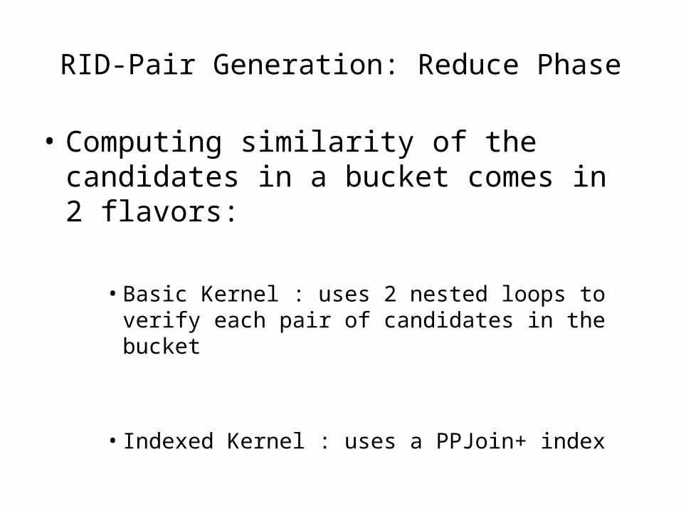
• Computing similarity of the candidates in a bucket comes in 2 flavors:

• Basic Kernel : uses 2 nested loops to verify each pair of candidates in the bucket

• Indexed Kernel : uses a PPJoin+ index

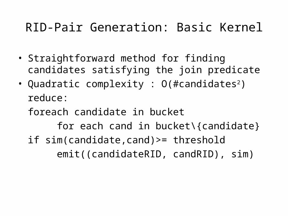
RID-Pair Generation: Basic Kernel

• Straightforward method for finding candidates satisfying the join predicate

• Quadratic complexity : O(#candidates2)

reduce:

foreach candidate in bucket

for each cand in bucket\{candidate}

if sim(candidate,cand)>= threshold

emit((candidateRID, candRID), sim)

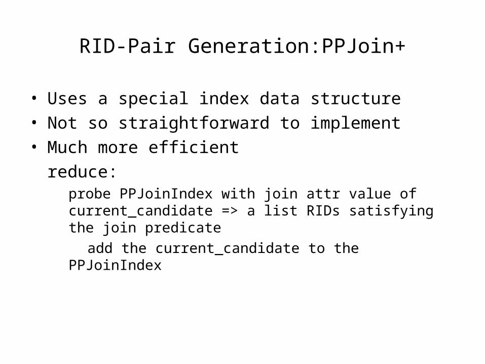
RID-Pair Generation:PPJoin+

• Uses a special index data structure• Not so straightforward to implement• Much more efficient

reduce:probe PPJoinIndex with join attr value of current_candidate => a list RIDs satisfying the join predicate

add the current_candidate to the PPJoinIndex

Stage III: Generate pairs of joined records


joined records


Stage II

Compute SSJoin&


good signatures

Stage I Stage III

Basic Record JoinBasic Record Join One Phase Record JoinOne Phase Record Join

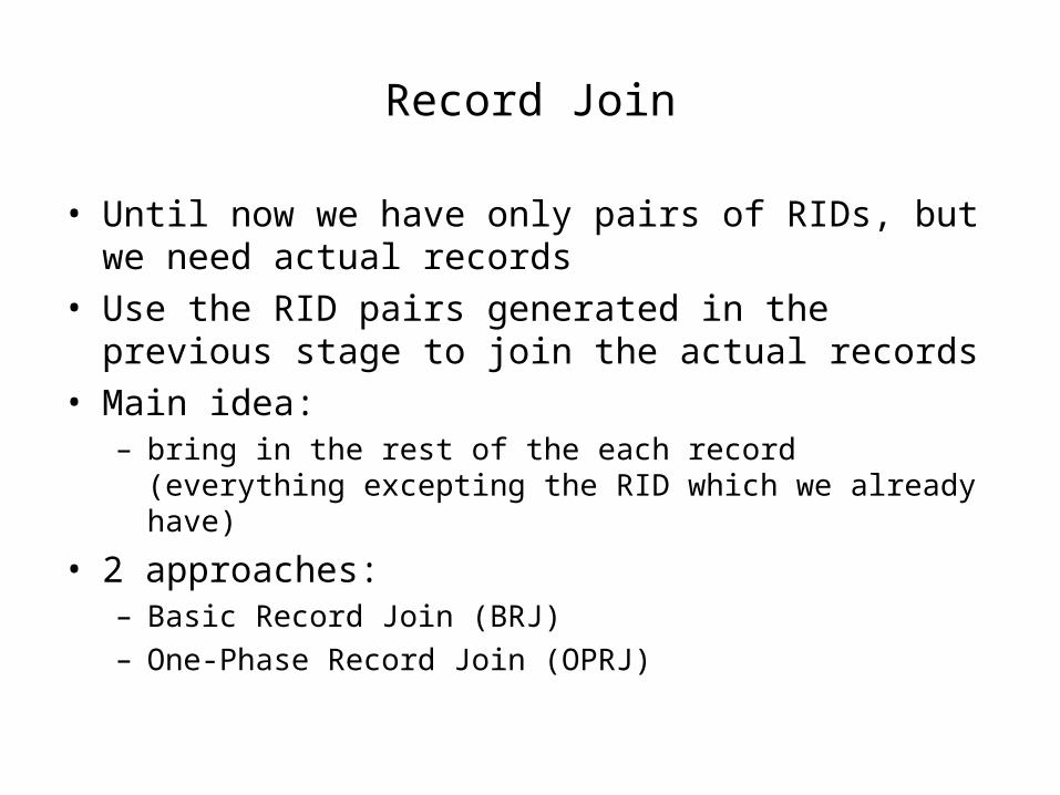
Record Join

• Until now we have only pairs of RIDs, but we need actual records

• Use the RID pairs generated in the previous stage to join the actual records

• Main idea: – bring in the rest of the each record (everything excepting the

RID which we already have)

• 2 approaches:– Basic Record Join (BRJ)– One-Phase Record Join (OPRJ)

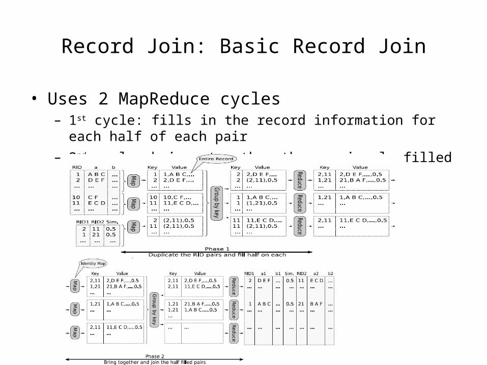
Record Join: Basic Record Join

• Uses 2 MapReduce cycles– 1st cycle: fills in the record information for each half of each pair

– 2nd cycle: brings together the previously filled in records

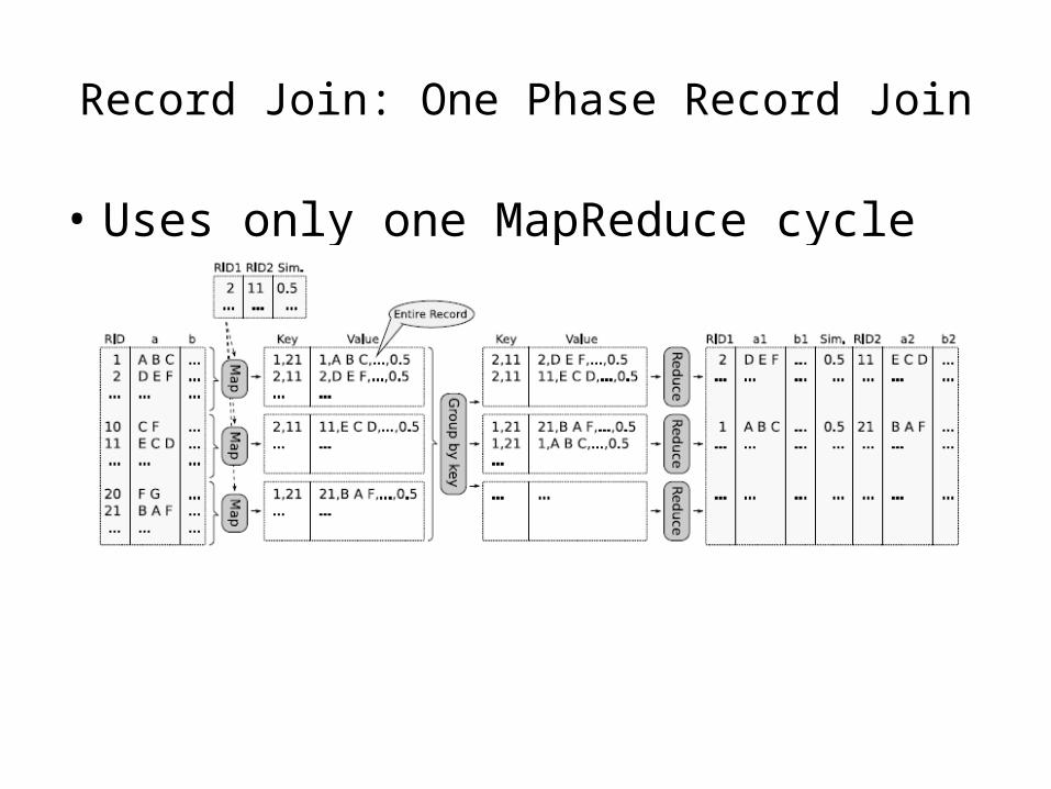
Record Join: One Phase Record Join

• Uses only one MapReduce cycle

R-S Join

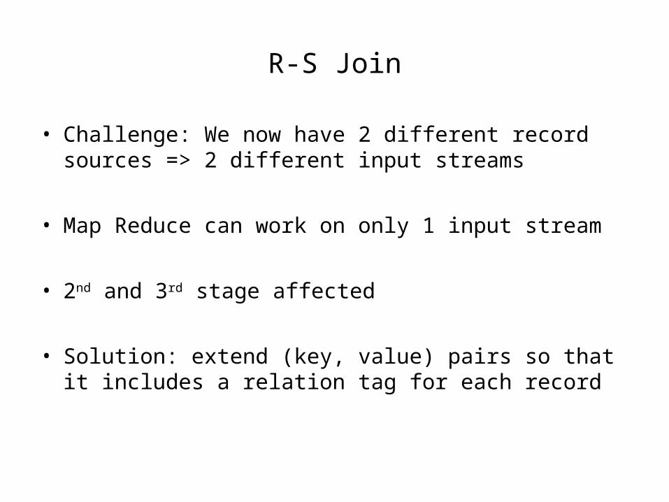
• Challenge: We now have 2 different record sources => 2 different input streams

• Map Reduce can work on only 1 input stream

• 2nd and 3rd stage affected

• Solution: extend (key, value) pairs so that it includes a relation tag for each record

Outline




• Evaluation

• Conclusions


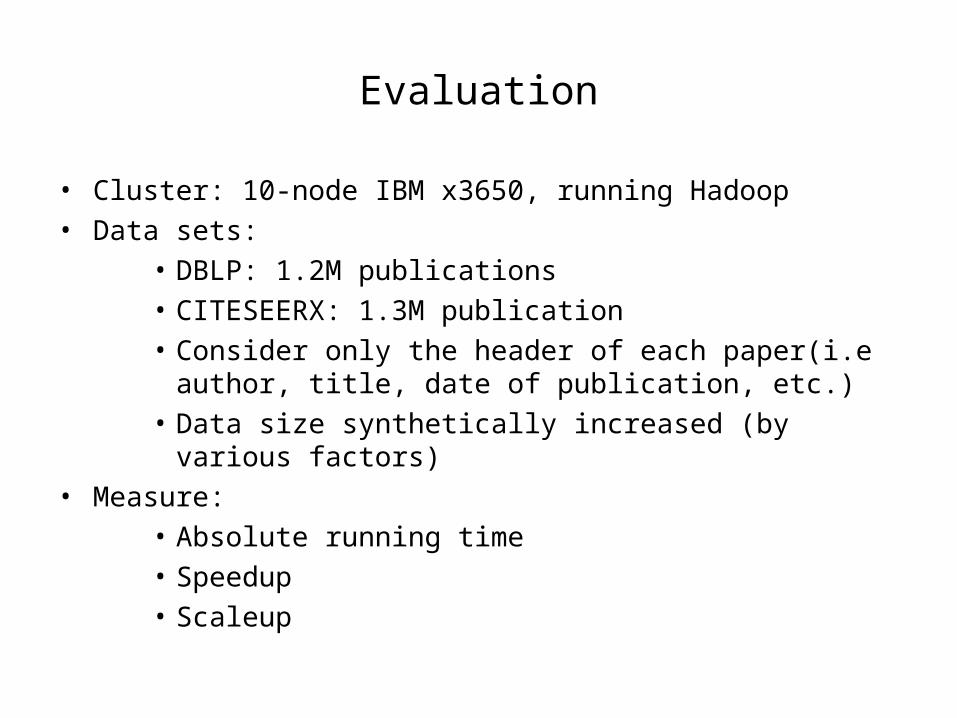
Evaluation

• Cluster: 10-node IBM x3650, running Hadoop• Data sets:

• DBLP: 1.2M publications• CITESEERX: 1.3M publication• Consider only the header of each paper(i.e author, title,

date of publication, etc.)• Data size synthetically increased (by various factors)

• Measure:• Absolute running time• Speedup• Scaleup

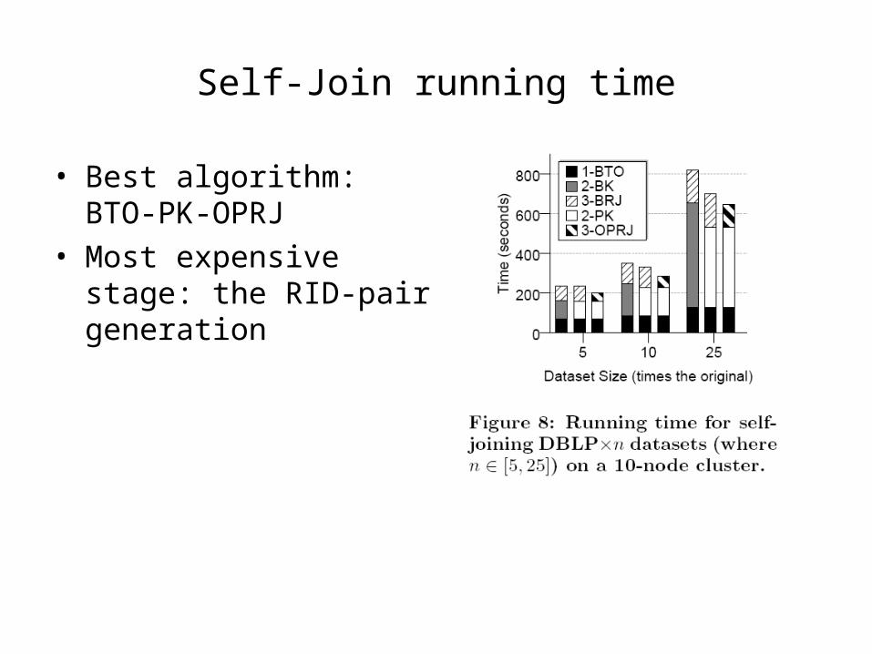
Self-Join running time

• Best algorithm: BTO-PK-OPRJ

• Most expensive stage: the RID-pair generation

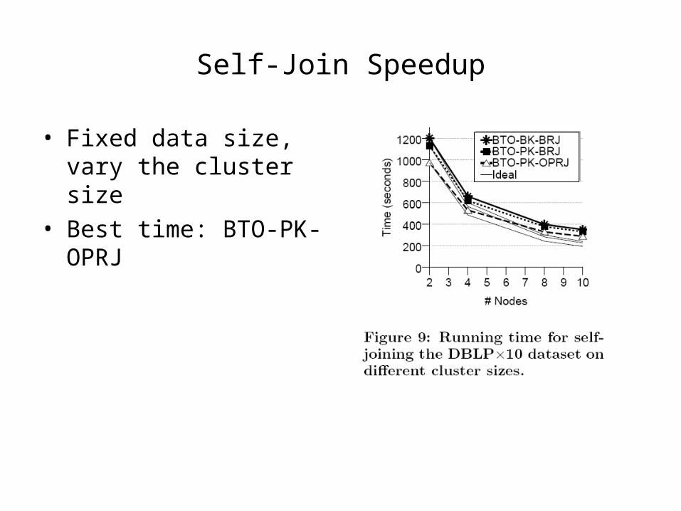
Self-Join Speedup

• Fixed data size, vary the cluster size

• Best time: BTO-PK-OPRJ

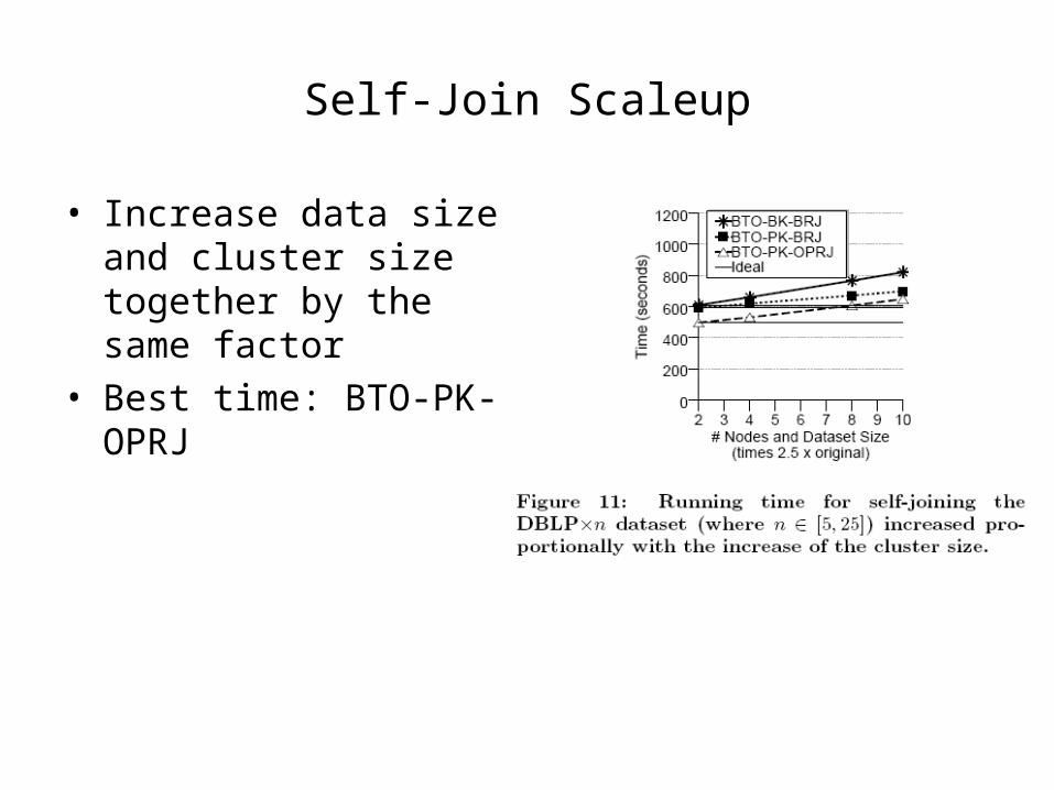
Self-Join Scaleup

• Increase data size and cluster size together by the same factor

• Best time: BTO-PK-OPRJ

R-S Join Performance

• Mostly, the same behavior

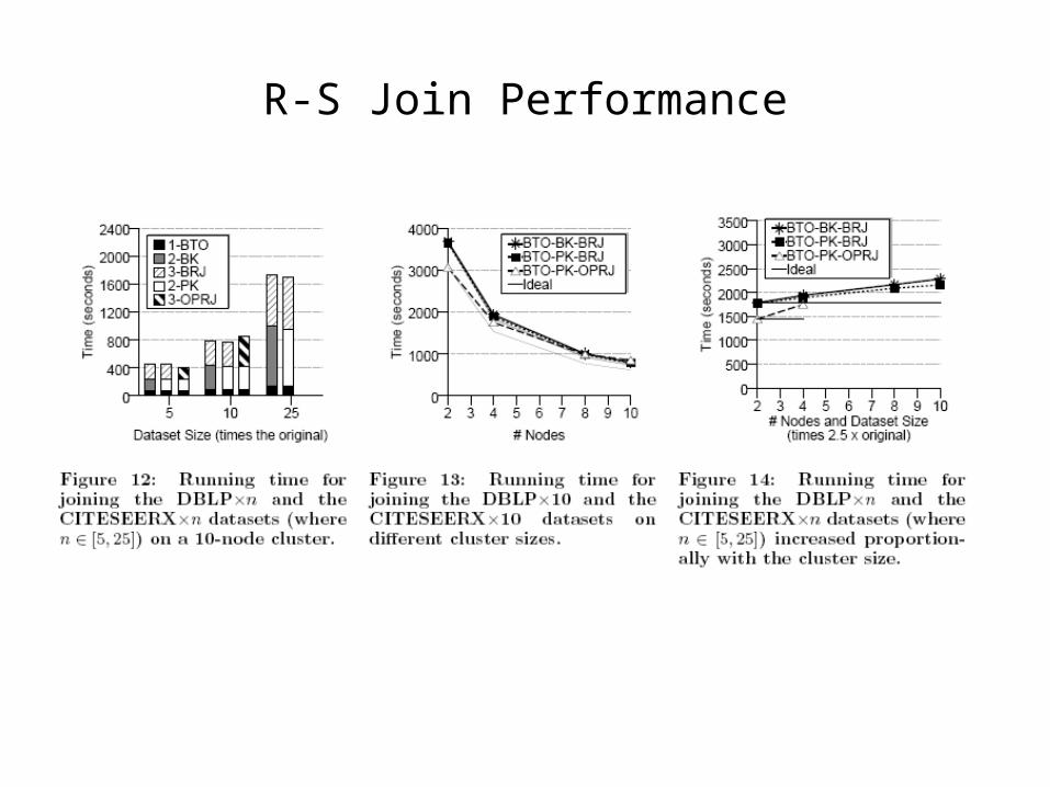
R-S Join Performance

Outline




• Evaluation

• Conclusions


Conclusions

• Efficient way of computing Set-Similarity Join

• Useful in many data cleaning scenarios

• SSJoin and MapReduce: one solution for huge datasets

• Very efficient when based on prefix-filtering and PPJoin+

• Scales-up up nicely

Strengths & Weaknesses

• Strengths:– More efficient than single-node/local SSJoin– Failure safer than single-node SSJoin– Uses powerful filtering methods (routing strategies)– Uses PPJoinIndex (data structure optimized for SSJoin)

• Weaknesses:– This implementation is applicable only to string-based input

data– Supposes the dictionary and RID-pairs list fit in main memory– Repeated tokenization– Evaluation based on synthetically increased data

Thank you!

Questions

efficient parallel set-similarity joins using mapreduce rares vernica, michael j. carey, chen li...

Documents

similarity metricfunction

similarity joinsimobj1

similarity joinmotivation2some

stringtext similarity

setsimilarity joinhow

similarity metric simo1

stringsimilarity joinsinput

obj2 obj1