efficiency aspects of government secondary school … aspects of government secondary school...
TRANSCRIPT
ISSN 1178-2293 (Online)
University of Otago Economics Discussion Papers
No. 1316
November 2013
Efficiency Aspects of Government Secondary School Finances in New South Wales: Results from a Two-Stage Double-Bootstrap
DEA at the School Level
Alfred A. Haug and Vincent C. Blackburn
Address for correspondence: Professor Alfred Haug Department of Economics University of Otago PO Box 56 Dunedin NEW ZEALAND Email: [email protected] Telephone: 64 3 479 5636
Efficiency Aspects of Government Secondary School Finances in New South Wales: Results from a Two-Stage Double-Bootstrap DEA at the School Level
by
Alfred A. Haug1 and Vincent C. Blackburn2
Abstract
This study measures the efficiency of government secondary schools in New South Wales, Australia, using a recently developed methodology of two-stage semi-parametric modeling. In contrast to previous research comparing school performance, we control for prior academic achievement of students by looking at the changes in academic achievements over a two year period, at the school level, from 2008 to 2010, and employ detailed financial data for deriving the envelope for the production frontier of the schools. Using Simar and Wilson’s (2007) double bootstrap procedure for data envelopment analysis (DEA), the study finds that schools with higher student retention rates, higher total student numbers, boys or girls only, and selective admissions do better than other schools. On the other hand, a negative influence comes from a school’s location in provincial and outer metropolitan areas, a higher ratio of disadvantaged students at a school, and a school’s specialization in areas such as languages, performing arts, sports, etc. A surprising result is that the socio-economic characteristics of the families of students attending the school has no significant effect on their academic performance, nor does the average of the years of service of the teachers at a specific school. JEL Code: C44, C61, H53, I21, I22 Key Words: Two-stage data envelopment analysis; double-bootstrap; efficiency of high schools in New South Wales, Australia. _____________________________________________________________________ 1. Professor and Head, Department of Economics, University of Otago, P.O. Box 56, Dunedin 9054, New Zealand. Phone: +64-3-479-5636. Email: [email protected] 2. Manager, Statistical Performance Reporting, Finance and Investment New South Wales, Department of Education and Communities, Level 9, 1 Oxford Street, Locked Bag 53, Darlinghurst, New South Wales, 2010, Australia. Phone +61-29-244-5277. Fax +61-29-244-5235. Email: [email protected]. The views expressed in this paper are those of the authors and not those of the Department of Education and Communities.
2
1. Introduction
Over the last decade increasing attention has been paid to greater efficiency and public
accountability of Commonwealth (federal) and State government funds devoted to school
education in Australia. Since the publication of ‘League Tables’ for individual schools on the
“My School” website of the Australian Curriculum Assessment and Reporting Authority
(ACARA), starting in 2008, the major debate in public education has focused on whether such
tables portray a complete picture of a school’s effectiveness in supporting children’s fullest
development potential.1 Critics have been arguing that the publication of ‘league tables’ may
lead to a market-based approach to education, resulting in the diversion of more government
money to non-government schools because conventionally state programs are generally
associated with low levels of allocative and technical efficiencies. The main argument is that the
lower levels of efficiency would lead to a lower level of resources and services offered by those
schools, which will limit the scope of reducing educational inequality, under-achievement, and
social de-segregation. In 2010, two-thirds of all children went to public (government) schools
and the combined Commonwealth and State funding for public schools was $26.3 billion and for
private schools $2.1 billion. The federal funding for public and private schools in 2010 was $2.5
billion and $5.5 billion, respectively (Hinz, 2010). Considering the amount of money spent on
public education, there is only a very limited number of studies available exploring how
efficiently the resources are being spent by the public schools in Australia.
The few studies that have measured cost efficiency for public schools in Australia using
state or national data are Mante and O’Brien (2002), Bradley et al. (2004) and Perry and
McConney (2010). However, as far as we are aware, no study has examined the effects of
school and non-school inputs, such as financial resources, teacher characteristics, family socio-
economic status and student composition, on student outcomes in the context of Australian
primary and secondary schools. The need for school efficiency studies as measured by the
academic performance of students in relation to the money spent on schooling, while considering
socio-demographic variables outside the control of the schools, has been recognized since 2008.
1 League tables are commonly created using student results from standardized tests. Schools are ranked according to their students’ results with highest scoring schools at the top. The tables are reported on the website “My School” at www.myschool.edu.au.
3
With the introduction by the Commonwealth Government of the “My School” website in 2008,
which reports student test scores and financial variables for each school, it has become more
important to measure the overall performance of each school and report a cost efficiency index
for public school funding policy. In addition, the recent Gonski Inquiry report into the funding
of Australian schools has increased the demand for well-constructed school efficiency studies
(Gonski, 2011). Furthermore, Bradley et al. (2004) found that unadjusted test scores reported in
the ‘league tables’ as signals of school performance in a quasi-market model are misleading and
will increase social segregation between schools.
This paper seeks to address some of the requirements for the future research directions
into school efficiency as outlined in the Gonski report. The focus of our paper is on the analysis
of New South Wales (NSW) school efficiency utilizing the two-stage double-bootstrap data
envelopment analysis (DEA) procedure, which is a production-function approach with multiple
inputs and multiple outputs. However, the DEA methodology is a methodology that does not
require the availability of all output and input prices and quantities, as is the case in traditional
production function analysis in economics. It is therefore ideally suited for the analysis of non-
profit public sector organizations that do not have a full set of prices available, such as schools.
Furthermore, the DEA approach allows for simultaneous multiple outputs. The two-stage
double-bootstrap DEA has previously been applied to New Zealand secondary schools by one of
the authors (Alexander et al., 2010). However, in contrast to that study, we have data that allows
us to control for prior academic achievement of students. The bootstrap method is used to bias-
adjust coefficient estimates and also for calculating proper confidence intervals for statistical
inference. Many previous studies reported large and imprecise confidence intervals (e.g., Miller
and Voon, 2011). The bootstrap method generally produces more precise confidence bands.
Our Australian data set covers the period from 2008 to 2010 and approximately 380 NSW
secondary schools and includes variables that have not been used in other studies on Australian
secondary schools. In the next section, we provide the background for this study including a
brief survey of previous studies undertaken in the Australian school finance literature.
4
2. The New South Wales Secondary School System
New South Wales operates a centralized system of funding for government schools. The
NSW State Budget process is the mechanism used to determine, monitor and control the overall
level of funding associated with the provision of school level education and training services.
Approximately 82.5% of school recurrent resources are from NSW state allocations.
Commonwealth government allocations make up 13%, this amount having grown since 2009
through increased federal funding under the Building the Education Revolution and National
Partnership programs (Keating et al., 2011). School derived revenue makes up about 4.5% of
school funding.
The expenditure that is incurred at the school level from these State and Commonwealth
allocations is met through two basic methods: (1) Central allocations of resources (including
staff) and funds that schools can utilize, and (2) direct central payments of school based costs.
The funding is provided through two core mechanisms, centralized staffing allocations and
grants which are either ‘tied’ or ‘untied’. The resources applied to schools can be categorized
into five categories: (1) staffing and salaries for school based staff (both teachers and school
administration and support staff (SASS), (2) global funding, (3) tied and untied grants, (4) capital
works and maintenance and (5) cleaning.
Staff positions in schools are allocated centrally on the basis of formulae, with some
capacity for variation based on negotiations between the school and Department of Education
and Communities. Schools may seek additional staff if they have a budget surplus. Staffing
constitutes about 81% of the operational costs of a school. The effective budget allocations,
using the same formula across schools, will vary due to the different salary steps of teachers. The
staffing formulae and the appointment and transfer systems are influenced by Enterprise
Bargaining Agreement outcomes. The classification of a secondary school and its principal is
based on total school enrolments, including regular class enrolments and student support
enrolments. The general teacher category is allocated separately upon the basis of Year 7-10 and
11-12 enrolments. Low socio-economic status (SES) schools also receive allocations under the
Priority School Funding Scheme. School Administrative Support Staff and Specialist Staff are
also allocated on the basis of student enrolments as are nonteaching staff, including a school
manager, administrative officers and general assistance staff. Global funding allocations are
5
calculated annually for each school at the beginning of each school year and at the
commencement of Semester 2 and are intended to help schools meet operational costs.
Special factor loadings are additional entitlements to compensate schools affected by
specific circumstances such as urgent minor maintenance and isolated location. A Global
Funding enhancement element also operates to take account of rural location and socio-economic
considerations. Beyond the above allocations a range of services and grants are delivered by
central and regional staff including school cleaning and maintenance and professional
development programs. Additional equity and needs allocations are also delivered to schools
mainly through the staffing formulae. Student population factors utilized include SES, English as
a second language (ESL) and New Arrivals, Indigenous, Isolated and Disability characteristics.
School circumstances recognized include location, enrolment size (diseconomies of scale) and
complexity. Factors that contribute the most are disabilities and SES dimensions. Allocations to
schools for capital works and maintenance are based on regular condition assessments and
facilities planning related to population growth conducted by NSW Department of Education and
Communities central staff.
The government in NSW recently announced a change of direction through devolving
decision making to school principals and school councils called the “Local Schools, Local
Decisions” initiative. To accomplish this transition a new Resource Allocation Model was
designed in mid-2012 for staged implementation from 2013 for 229 schools, with the balance of
the other 2,000 schools being incorporated by the end of 2015. By that time schools will manage
more than 70% of the total NSW school education budget. The efficiency modeling contained in
this paper using school input and output data for 2008-2010 should be a very useful prior tool to
evaluate the impact of the subsequent devolution of school budgetary and staffing on variations
in school efficiency levels. It is hoped that this study will lead to a series of “before” and “after”
assessments of the intended improvement in school performance and to greater “value for
money” in schooling arising from such reforms.
3. Background and Literature Review
In the Australian context of schooling most studies exploring school effectiveness focus
on the bivariate relationship between the socio-economic status of students or schools and
6
academic achievements. For example, Perry and McConney (2010), using data from the 2003
Program for International Student Assessment (PISA) for Australian students, compared
quintiles of the mean performance scores in each of reading, mathematics and science for
individual student SES to those for school group average SES. They found: (1) increases in the
mean SES of a school are associated with consistent increases in student academic achievement,
(2) the relationship between school SES and academic achievement is similar for all students
regardless of their individual social background, and (3) the strength of the relationship between
school SES and achievement increases as the SES of the school goes up. Furthermore, they
analyzed the relationship of each performance score to gender, individual SES and school-level
SES with three hierarchical regression analyses and argued that each contributed “…for
independent and unique portions of variance, over and above that accounted for by gender, in
reading, math, and science achievement...” (p. 1150). However, other potential predictors
(explanatory variables) are not considered and it is not obvious what hierarchical order should be
used for the inclusion of predictors. Indeed, Marks (2010) also used 2003 PISA data in order to
examine school-level effects on student performance for tertiary entrance in Australia and found
opposite results with respect to the role of SES. He controlled for schools’ academic context and
found (p. 267) that “The socio-economic context of schools has no effect on student performance
when taking into account schools’ academic context.”
An earlier study by Mok and Flynn (1996) analyzed a sample comprising 4,949 Year-12
students from randomly selected NSW Catholic high schools suggested that students from larger
Catholic high schools, on average tended to achieve more highly than their peers from smaller
schools, even after controlling for students’ background, motivation and school-culture variables.
The estimation method used accounts for intra-class correlations due to clusters of students
coming from the same school. Mok and Flynn (pp. 77-74) pointed out in their conclusion that
two “powerful predictors” were unavailable for their study: students’ ability and previous
academic achievements. They acknowledged that the inclusion of these two variables in their
analysis might lead to the variable measuring school size becoming statistically insignificant and
that “a carefully mapped list of control variables” is needed for further research on Australian
high schools.
The first study on school efficiency in Australia by Mante and O’Brien (2002) assessed
the technical efficiency of 27 Victorian secondary schools in 1996 using the Charnes et.al.
7
(1986) DEA model. Mante and O’Brien used a one-stage regression DEA model with only one
or two inputs. In contrast, we use a two-stage regression DEA model with multiple inputs in
stage one and multiple environmental controls in stage two and we also apply double
bootstrapping in order to get unbiased results. Nevertheless, their paper provided a good
discussion of the advantages of applying DEA to public-sector non-profit organizations (schools)
for performance evaluation when input and/or output prices are unavailable so that a standard
empirical production function cannot be specified. Mante and O’Brien found that most of the 27
schools were in a position to increase their outputs through a more efficient use of their available
resources.
Bradley et al. (2004) discussed the role of league tables in providing signals and
incentives in a school education quasi-market framework. They compared a range of unadjusted
and model-based league tables for primary school performance in Queensland government
schools. Their results indicated that model-based tables which account for SES and student
intake quality vary significantly from the unadjusted tables. On the other hand, a report for the
Victorian Department of Premier and Cabinet (Lamb et.al. 2004) examined the effects of core
funding, locally raised funds and a number of special sources of funding (English as a Second
Language or ESL funding) together with variables measuring teachers’ background using multi-
level models. They concluded that the resource variables had positive effects on student
outcomes, though these effects were small, generally statistically insignificant and varied
between outcome measures examined.
Miller & Voon (2011) examined Australia’s National Assessment Program – Literacy
and Numeracy (NAPLAN) results for 2008 and 2009 using the education production function
methodology of the type popularized by Hanushek (1986). Test score data for 3rd, 5th, 7th, and 9th
graders were regressed against SES characteristics, type of school, percent of female students,
student attendance, school size, and state and region. They applied mostly least squares
regressions with a heteroscedasticity adjustment for the standard errors of the regression
estimates. In order to explore differences across school types (government, independent and
Catholic schools), they used an Oaxaca (1973) decomposition. They found large differences in
educational outcomes by state and school type. Their findings indicated that some schools had
academic achievements both better and worse than their other characteristics would suggest.
Their study did not include variables measuring school resources and they suggested that future
8
studies should include such variables. However, Miller and Voon (forthcoming) examined the
issue of different outcomes across states further, using regression discontinuity analysis in order
to account for school distance from the state boundary for NSW and Queensland. They used a
similar specification with NAPLAN data for Year 3 in 2009 and found that institutional and not
state effects account for the different performance outcomes in these two states.
The major objectives of our study are: (1) to identify those New South Wales schools that
are inefficiently managing their resources while delivering the state mandated educational
outcome; and (2) to identify the factors which account for efficiency differentials among schools.
To achieve these objectives, we define and estimate a two-stage double-bootstrap DEA. To the
best of our knowledge, this model has not yet been applied for measuring cost efficiency for
Australian public schools. Also, in contrast to a related study for New Zealand (Alexander et al.,
2010), we control for prior academic achievement of students. We consider our two-stage DEA
approach as novel for Australian data.
4. Econometric Methodology
We apply two-stage data-envelopment analysis (DEA) with the double bootstrap. DEA
is a linear programming technique to construct a model that measures the efficiency differences
between schools.2 Each school is treated as a decision-making unit in this setup. Schools are
compared to each other in terms of their efficiency in transforming a given set of inputs into
outputs. One advantage of DEA is that it allows for multiple outputs, without having to make
assumptions about “firm” (school) behaviour such as profit maximization or cost minimization.
It means that there is no need to construct a composite single output, which would be difficult in
our case because the outputs do not have clearly defined market values and the choice of weights
for combining outputs would be difficult. Another advantage of DEA is that it is not necessary
to specify the mathematical form of a production function because DEA is a non-parametric
method (in its first stage, the DEA stage). In particular, we do not need input and output prices 2 Worthington (2001) provided an explanation of DEA and a review of empirical studies applying it to schools. Cook and Seiford (2009) surveyed DEA advancements over a thirty year period. Recent applications of DEA analysis include, among many others, Alexander et al. (2010) to study New Zealand secondary school efficiency, Barkhi and Kao (2010) to appraise the performance of decision making tools in information science, Erhemjamts and Leverty (2010) and Cummins et al. (2010) to analyze the efficiency in the insurance industry, and Chang et al. (2004) to assess the operating efficiency of hospitals.
9
as is the case for standard parametric production functions. DEA allows us to identify the group
of the most efficient schools that inefficient schools should ideally follow in order to become
efficient by adopting their best practices for managing a school. In contrast to estimations of
production functions with methods related to least squares or maximum likelihood, DEA
produces an envelope around the production points on the production frontier instead of focusing
on an average of production points.
The DEA involves a second stage parametric regression in our application, i.e., it is a
two-stage semi-parametric DEA. The second stage regression assesses the factors that determine
the differences in the efficiency scores of each school as calculated from the first stage DEA.
The second stage involves truncated regression analysis, due to the limited range of the
efficiency scores (between 0 and 1) and some lumpiness in the estimated values (due to several
values of 1 for the most efficient schools). The second stages explains the efficiency score
differences as a function of environmental factors, such as school location, type of school (boys
only, girls only, or mixed gender) and other variables that are not inputs in the production
process per se.
Simar and Wilson (2007) gave a long list of two-stage DEA studies applied to efficiency
analysis in different setting. However, they criticised almost all of those studies, including those
on school efficiency, because they ignored serial correlation in the DEA efficiency estimates
leading to biased inference. They also pointed out that a naive bootstrap for correcting for serial
correlation is inconsistent due to the non-parametric nature of the efficiency estimates. We
therefore follow the double bootstrap methodology as outlined by Simar and Wilson (2007).
This method bias-adjusts the efficiency scores with the bootstrap method and allows for
conducting consistent inference for the effects of environmental variables on school efficiency,
using again the bootstrap method in connection with truncated regression analysis.
The importance of the second bootstrap that is applied by Simar and Wilson (2007) in
order to calculate accurate confidence intervals is illustrated by several previous studies on
school performance, though they generally used different estimation methods. Miller and Voon
(2011) explained that their relatively large confidence intervals (or bands) are in line with other
research assessing the effects of school factors on student performance. Such large and
imprecise confidence intervals may lead a researcher to incorrectly conclude that a factor has no
statistically significant influence on student performance because the, say 95%, confidence band

10
includes zero. Such a result could then, for example, be used to argue that a policy that focuses
on the schools that disadvantaged students attend, instead of focusing on the individual
disadvantaged students directly, is misguided as it will not improve the performance of the
schools attended by the disadvantaged students so that there is no benefit to them. Therefore,
bootstrap-based confidence bands in the second-stage regression of our DEA model, where we
determine the significance of the influence of environmental variables, are necessary in order to
avoid biased statistical inference.
Farrell (1957) defines efficiency with an input orientation so that input efficiency is
measured for a given level of outputs. Efficiency is measured as the radial distance while
keeping fixed the direction of the input vector to the production frontier. We allow for variable
returns to scale. For DEA, the unobservable production frontier is estimated by linear
programming, with the observed data on schools. For each school an efficiency score is
estimated that ranks the school relative to the estimated frontier, i.e., relative to the most efficient
schools in the sample.
Simar and Wilson (2007) described the statistical assumptions needed in order to derive
the properties of the DEA estimator that leads to logical consistency for the second-stage
regression involving the environmental variables. They also specified the separability conditions
for the two-stage procedure. The second stage regression involves a censored variable, the
efficiency score. Furthermore, the second stage truncated regression involves a generated
regressor and the efficiency scores are also correlated in an unknown fashion. Simar and
Wilson’s (2007) methodology overcomes these problems by applying a double bootstrap to a
well specified statistical DEA model.
A major drawback of the standard DEA method had been that it is deterministic and does
not allow for random influences so that any deviations from the production frontier are assumed
to be due to inefficiency. Standard DEA analysis could therefore not accommodate
measurement error or other random fluctuations. The recent methodological advance by Simar
and Wilson (2007) with bootstrap sampling solved this problem. The construction of proper
confidence bands for estimated efficiency scores and a statistically correct second-stage DEA
analysis became possible.
We use the statistical software package FEAR 1.15 of Wilson (2008) in connection with
programming language R, version 2.12.0. Efficiency can be measured in terms of Shephard’s
11
(1970) input distance function that is the reciprocal of Farrell’s measure. Shephard’s measure is
therefore one or larger, and Farrell’s measure is one or less. The results of Kneip, Park and Simar
(1998) can be translated into Shephard’s distance measure in a straightforward manner. The
simplex method of Hadley (1962) is used in order to calculate the distance function estimates for
the DEA efficiency estimates.
We program in R the double bootstrap following Algorithm No. 2 in Simar and Wilson
(2007). First, we use the DEA procedure in FEAR to estimate Shephard’s efficiency scores for
each school in a given year. Second, we carry out the truncated normal regression by maximum
likelihood estimation, regressing estimated efficiency scores that are larger than one on the
environmental variables. We use the “treg” command in FEAR. Third, we program a bootstrap,
drawing 100 samples each of size 345, from the truncated empirical normal distribution of the
estimated efficiency scores.3 We use the pseudo-random-deviates generated with “rnorm.trunc”
in FEAR. Fourth, we calculate the bias-corrected efficiency scores with the bootstrap method.
Fifth, we use the bias-corrected efficiency scores to re-estimate the marginal effects of the
environmental variables in the second stage regression. Sixth, we apply a second, the so-called
double, bootstrap using the empirical distribution of the bias-corrected second-stage regression.
We obtain 5,000 replications for each parameter estimate of the marginal effect of environmental
variables. We also experimented with 10,000 replications but there were no improvements
compared to 5,000 replications. Last, we calculate bootstrap-based 95% confidence intervals for
each parameter estimate.
4. The Data
In NSW there are, depending on the year one looks at, approximately 380 government
(public) secondary schools in the data set, of which about 45 are selective (or partially selective).
Parents can enter their children to a “selective school” entrance examination at the end of
primary school, thus allowing selective schools to get the highest achieving primary students into
these government secondary schools (the selective schools contain the three agricultural high
schools in NSW). Another approximately additional 50 secondary schools are “specialist” high
3 Using instead 200 observations did not affect the results in any meaningful way. This is consistent with Simar and Wilson (2007, page 14), who found that 100 replications are “typically sufficient.”
12
schools (languages, performing arts, sports, technology, etc.). The remainder of the secondary
schools are non-selective and non-specialist “comprehensive” high schools (about 285 schools).
The data for this study come from the Departmental Annual Financial Statements in the
state of NSW. The original dataset contains detailed information on several inputs, outputs and
other socio-economic variables for all primary and secondary schools in NSW. For school
outputs, we relied on two measures. The first measure takes the test performance of students
who are in Year 12 in 2010 and compares it to their test performance two years earlier, in 2008
when the same cohort was in Year 10. The second measure takes the test performance of
students who are in Year 9 in 2010 and compares it to their performance two years earlier when
they were in Year 7. In other words, we want to measure how much a school contributed to
learning of its students over a two year period. Students enter high school with different
academic achievements. A school’s performance should be measured in terms of what it adds to
student achievement, controlling for the differences in numbers of teachers, support staff, and
students, spending on teacher and other staff salaries, as well as differences for other
expenditures such as maintenance and cleaning, all on a per-student basis.
Previous research (e.g., Marks et al. 2001) found that prior academic achievement is one
of the main, if not the main, determinant of academic achievement. It is therefore most
important to control for prior academic achievement of high school students, in particular when
comparing the efficiency of high schools in transmitting new academic knowledge to students.
We follow the approach of Lamb et al. (2004), among others, and look at the test scores of a
cohort of students in 2010 and the same cohort’s prior academic achievement two years earlier in
2008. Students in Year 12 in 2010 were in Year 10 in 2008, and students in Year 9 in 2010 were
in Year 7 in 2008. Lamb et al. (2004, p.29) pointed out, in the context of schools in Victoria,
that the cohort two years earlier contains many of the same students. Miller and Voon (2011)
also discussed the importance of this issue but could not follow this approach due to data
unavailability. They included instead in their study Year 3 achievements in 2009 as a proxy for
2009 Year 5 students’ prior academic achievement and stated (p. 377) that “… our measure
should be viewed as only a crude proxy for prior academic achievement.”
13
We use a school’s median Year 12 Higher School Certificate university entrance
“Australian Tertiary Admission Rank” (ATAR) results in 2010.4 We compare this result to that
of the same cohort in 2008 when the cohort was in Year 10.5 A school’s 2008 median Year 10
School Certificate exam result is used.6 For these two tests, the median is reported for every
high school but the averages are not reported.7 Next, we standardize for each school every test
score by subtracting the mean across all schools in the sample and dividing the result by the
associated standard deviation. Then, we take the standardized ATAR score (dated 2010) minus
the standardized Year 10 score (dated 2008) and use the result as one of the two output measures.
The standardization makes the two tests comparable. Also, this way we focus on the “average
student” at a school.
The second output measure uses the average NAPLAN test scores for Year 9 in 2010 and
the average NAPLAN test score for Year 7 in 2008. We apply the same standardization and
subtract the Year 7 score from the Year 9 score to get our second measure of school output.
Median school scores are not reported in the official statistics for the Year 9 and 7 tests at the
school level so that we have to rely here on the averages instead.
The unit of measurement that we use for outputs as well as inputs is the individual
school. The inputs used for the first-stage DEA are for the year 2010 the full-time-equivalent
number of teachers, of student-support staff, the average contract salary for teachers and for
support staff, the school’s “own” expenditures plus all other school operating expenditures such
as insurance, maintenance and cleaning. A school’s own expenditure refers to school
expenditures derived from the school’s own income sources that include, for example, the
school’s interest income from bank balances. All these input variables are defined on a per-
student-basis: we divided each variable by the total number of all full-time equivalent students
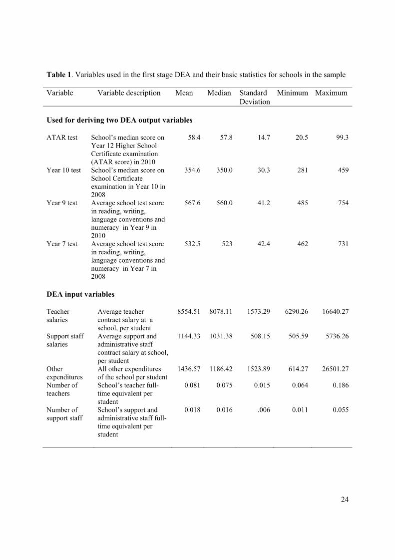
enrolled at Years 7 to 12. Table 1 lists the variables and abbreviations used in the first stage,
along with basic statistics. 4 NAPLAN is the “National Assessment Program – Literacy and Numeracy” initiative of the federal government that started in 2008 for every school in Australia. In Year 12 the Higher School Certificate overall median exam results are summarized in the ATAR scores, which are used to measure university entrance into undergraduate courses. 5 Of course, there are students who migrate to another school and others who join as new students as we go from 2008 to 2010. This introduces some measurement error, though we believe that the effects from migration are minor and possibly random. Unfortunately, migration adjusted data are not available. 6 At Year 10, the last year of compulsory schooling, the school’s median for the NSW School Certificate is reported for the exam average over five subjects. 7 Table 1 provides detailed statistics for all test scores that we use in our analysis.
14
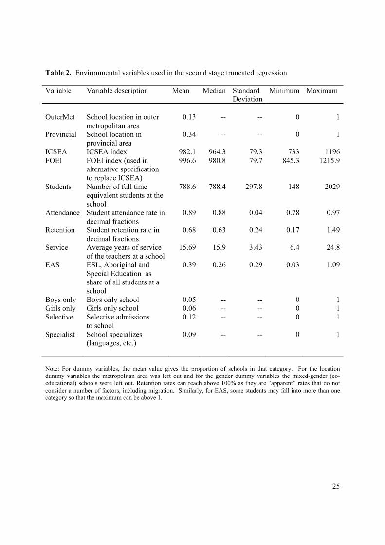
The variables used to control for the school environment in the second stage truncated
regression of the DEA analysis for the year 2010 are listed in Table 2. Our data source reports
school locations for the following areas: inner metropolitan, outer metropolitan, inner
provincial, provincial with 50,000 to 99,999 inhabitants, provincial with 25,000 to 49,999
inhabitants, outer provincial, remote and very remote. We consider three areas only: inner
metropolitan, outer metropolitan and provincial, where the latter summarizes all others. We pick
therefore two dummy variable, namely outer metropolitan and provincial.
The socio-economic status of the students is measured by an index called “Index of
Community Socio-Educational Advantage” (ICSEA) computed by the Australian Curriculum
Assessment and Reporting Authority (ACARA, 2010). The index is available for all schools
across all six states and two territories in Australia. The mean index is 1000, implying schools
above this number are declared to be more advantaged, and those below are less advantaged.
Miller and Voon (forthcoming) considered in their study four alternative measures for the social
and economic standing of areas as constructed by the Australian Bureau of Statistics and found
that ICSEA is “by far the better predictor” (p. 6) for the variance in aggregate school outcomes
that they analyzed. Nevertheless, we considered an alternative index of socio-economic status,
the Family Occupation and Education Index (FOEI), developed only for NSW schools by the
NSW Department of Education and Training. The correlation coefficient for the two socio-
economic indices is 0.97. We applied the FOEI instead of the ICSEA as part of our robustness
analysis and report results in Section 6.3 below.
We use the number of full-time equivalent students to measure school size effects and the
squared number of students to capture any scale economies at the school level. Other
characteristics of schooling controlled for are apparent retention rates of students8, student
attendance rates, and teachers’ average years of service. The latter is a proxy for teacher
experience, assuming that more teacher experience increases a teacher’s effectiveness with
regards to transmitting academic knowledge to students. Further, we include the decimal
fraction of students enrolled in English as a second language or with a language background
8 Retention rates are “apparent” rates that do not track individual students through to their final year of secondary schooling. They measure the ratio of the total number of full-time school students in a given year divided by the total number of full-time students in the previous year. The base year is Year 7, when secondary school starts in NSW. It is possible to have apparent retention rates above 100% because of a number of factors not considered, including migration.
15
other than English, the fraction of students in special education, and the fraction of students with
Aboriginal status. We combine the three categories (labeled “EAS”) because there are
insufficient numbers in the last two categories to separate them out. We also control for the
schools admitting boys or girls only, for having selective admission, and for schools specializing
(Specialist High Schools). We collected information on all variables for all secondary schools in
NSW. However, non-availability of exam results data and missing information on some other
variables prohibit us to include them all in the sample. As a result, the current data set used
contains information on 345 secondary schools.
6. Empirical Results
6.1 First Stage Bootstrap-Adjusted DEA Results
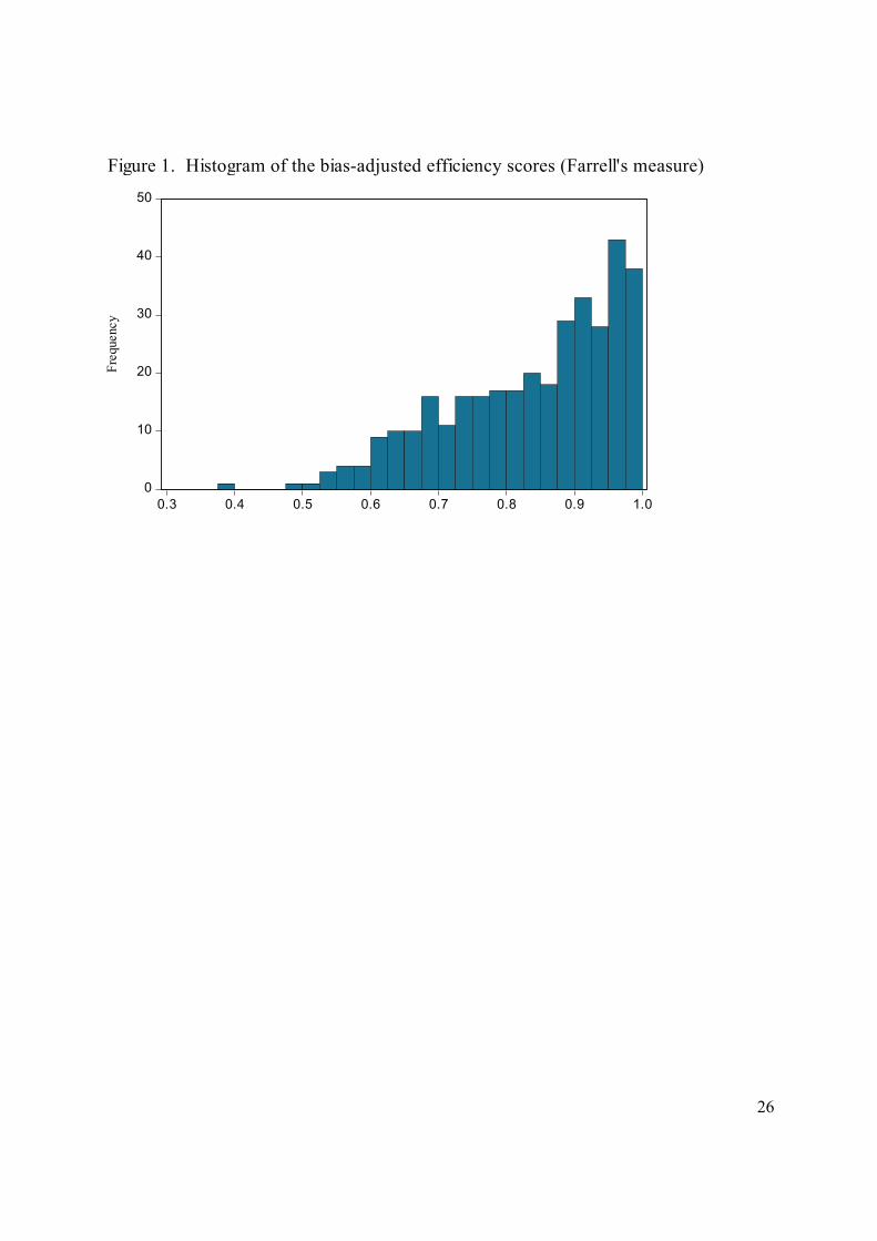
Figure 1 depicts the histogram for the calculated bias-adjusted efficiency scores in stage
one of the analysis, the DEA stage that derives the production frontier envelope. Efficiency is
measured with respect to how much a school adds to average student knowledge, given its
available inputs per student in terms of teachers, other staff, and money. It is important to note
that we do not look at the output in terms of median or average test score results achieved by a
school in a given year. Instead, we assess how much a school changes test scores, on average,
relative to all other schools for a cohort of students over a period of two years of schooling. In
other words, we measure which schools use the best practice to deliver the most improvements in
student learning as measured by test outcomes. Efficient schools that use the inputs most
efficiently are on the production frontier and get assigned a score of 1. Schools that are
inefficient get a score of less than one, using Farrell’s measure. Of the 345 schools analyzed, 8
schools achieved a perfect score of 1.00 and altogether 24 schools have an efficiency score of
0.99 or higher. In total, 144 schools scored at or above 0.90. At the lower end, the three lowest
efficiency scores are 0.38, 0.50 and 0.51. There are 12 schools with scores below 0.60.
It is interesting to note that the ranking based on the bias-adjusted efficiency scores is
very different from a ranking based on the raw scores for ATAR or for Year 9 tests taken in
2010. This is also evident from the small correlation coefficient of 0.54 between the efficiency
and ATAR scores and of 0.49 between the efficiency and Year 9 scores. On the other hand, the
correlation coefficient between ATAR and Year 9 test scores is 0.85, which is much closer to 1.
16
This means that controlling for resources available to individual schools, and looking at the
academic improvements of students achieved by a school, changes the position of a school in
league tables compared to that solely based on raw test scores. In other words, not all schools
have the same resources available (inputs used in our analysis) and schools differ in how much
value they add to an average students’ education. The efficiency scores account for these
differences, whereas the raw scores do not. Of course, there are other factors besides the inputs
that affect the differences in the efficiency scores among schools. We consider these factors next,
in the second stage of the DEA.
6.2 Second Stage DEA Results for the Truncated Regression
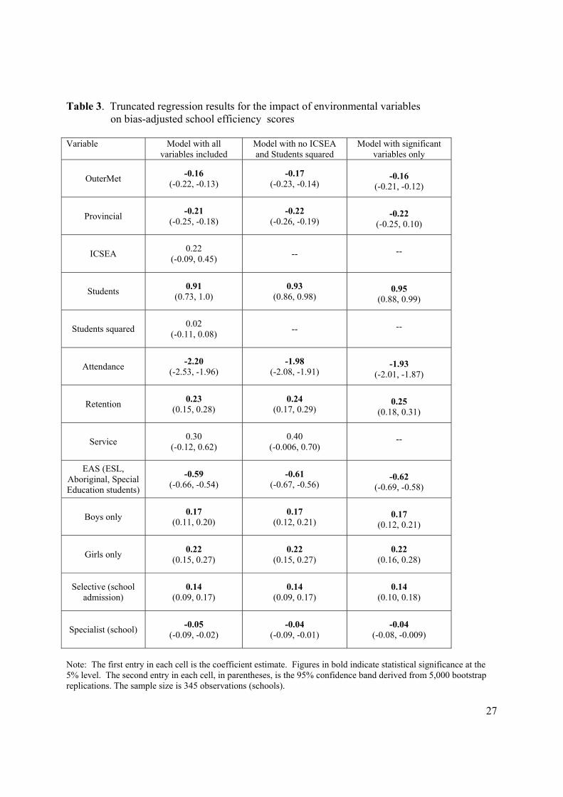
The second stage results for the effects of the environmental variables on the bias-
adjusted efficiency scores are reported in Table 3. Table 2 explains and gives detailed statistics
for the variables used in this stage. There are six categorical variables relating to school location
and type that are used to assist in explaining school efficiency differences. For location
identifiers we include two school-type dummy variables, setting for each outer metropolitan and
provincial area locations to 1 and other locations to 0. The category left out is inner
metropolitan. Other dummy variables are used to examine the relative performance of boys and
girls only schools. The category left out here is mixed gender (co-educational) schools. It is
expected that both these variables (boys only and girls only) will exhibit positive coefficients in
the regression results, thereby providing evidence of a school-level gender effect. The quality of
students is an important input to a school’s production process enabling assessments to be made
of a school’s efficiency in terms of the value it adds to its students’ academic knowledge. In
cases where schools are able to select students for entry at Year 7 on the basis of a competitive
entrance exam at the end of Year 6, such schools should exhibit greater success in terms of
subsequent examination results in Year 10 and Year 12. To capture this effect a dummy variable
was used for NSW Selective High Schools. We also control for NSW Specialist High Schools,
all relative to other “comprehensive” high schools.
A proxy for student quality commonly used is a socio-economic status indicator, whereby
a higher composite index value indicates a school with higher SES student backgrounds and vice
versa. We use two indexes, the Commonwealth designed ICSEA measure and the NSW designed
FOEI measure. Both measure, in slightly different ways, parental income, education and
17
employment characteristics. Their correlation coefficient of 0.97 indicates that either measure
could be included in the second stage regression. School size characteristics are also examined
for their effect on efficiency, reflecting underlying economies or diseconomies of scale in school
operations. To capture these effects we enter the variables “Students” and “Students squared”
(the square of “Students”). The school finance literature surprisingly finds little impact of
teacher quality on student achievement (Hanushek 2003). Our summary measure of teacher
quality (experience) is the average years of service of full time teachers, “Service”. Other
variables used in the second stage are indicators of student attendance (“Attendance” rate),
apparent student retention (“Retention” rate), and the decimal fraction of English as a Second
Language, Aboriginal and Special Education students (“EAS”) in a given school.
The second stage regression equation takes the form:
Bias-adjusted_efficiency_scorei = a0 + a1 OutMeti + a2 Provinciali + a3 ICSEAi +a4 Studentsi + a5 Students_squaredi + a6 Attendancei + a7 Retentioni + a8 Servicei + a9 EASi + a10 Boys_onlyi +a11 Girls_onlyi + a12 Selectivei +a13 Specialisti + ui (1) The subscript “i” refers to the ith school, the aj are the parameters to be estimated and ui is the
truncated regression error term. Table 3 presents the results. The second column gives the
results for equation (1) that show to what extend an environmental variable explains the variation
in differences of schools’ efficiency scores. First, we use the bootstrap-calculated 95%
confidence bands, reported in parentheses in each cell below the coefficient estimate, to find out
which variables have a statistically significant influence on efficiency. The most interesting
result is that the socio-economic background of students (ICSEA) has no statistically significant
effects, even though the effect is positive. This result is consistent with the findings of Marks
(2010), among others. In addition, we find that the variable “Students squared” has no
statistically significant effects. As we allow for variable returns to scale in the DEA, this is to
be expected. It confirms that the DEA model captures adequately the school size effects with
respect to economies of scale. The only other variable that has no statistically significant effect
is the variable “Service” that we used as a proxy for teacher quality. It may well be a poor proxy
and teacher experience in terms of average years of service may not reflect teacher effectiveness
in adding to student knowledge. Unfortunately, we do not have any other measure of teacher
effectiveness available beyond the extent to which it is captured already by salaries in the first
stage of the DEA.
18
We exclude the statistically insignificant variables from the model. We first delete only
ICSEA and “Students squared” and leave “Service” in the regression to check the sensitivity of
our results to model specification in terms of including a variable that should not matter. Indeed,
the results in column 3 of Table 3 are very similar in magnitude to those in column 2 and also to
those in the last column. Our model seems robust in this respect.
Table 3 lists in the last column the results for the models with only statistically significant
variables included. We label this our baseline model. Compared to column 2, the results are
very similar for the included factors. The location of a school has a significant influence on
school performance. A school located in an outer metropolitan or in a provincial area is at a
disadvantage. The coefficient estimates for these two variables show a negative impact.
However, the magnitude of the negative effect is about 38 percent larger in absolute terms for
provincial schools than for outer metropolitan schools, with both effects measured relative to
inner metropolitan schools. The size of a school in terms of student numbers has a positive
effect on school efficiency. It may be the case that larger schools can offer more specialized
courses and a “richer” curriculum that improve student learning. One puzzling finding is that
student attendance rates have a relatively strong negative influence on school efficiency. One
would have expected a positive impact. Attendance may be a measure that is quite imprecise and
inconsistent across schools in the way it is recorded. Literally interpreted it would imply schools
that “enforce” attendance create a school atmosphere that hinders learning. Admittedly, we do
not have a good explanation for this empirical result. On the other hand, student retention has a
significant positive effect, as one would expect. The effect of EAS is negative and quite large in
magnitude. EAS measures the share of ESL, Aboriginal and Special Education students in a
school’s total student body. Schools with higher proportions of EAS students show lower
efficiency outcomes. Schools that cater to boys or girls only, or have selective admission, have
better efficiency score outcomes. Girls-only schools fare much better than boys-only schools.
On the other hand, Specialist Schools have worse efficiency results, though the effect is quite
small in magnitude.
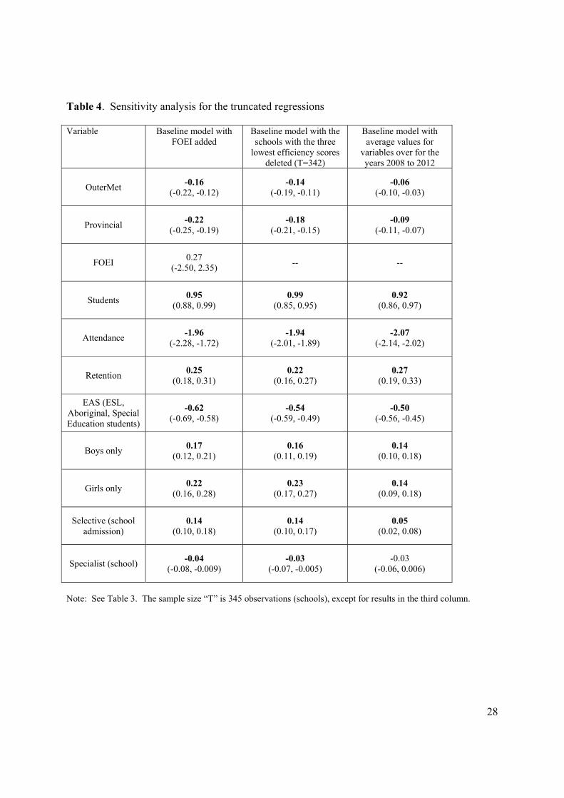
6.3 Robustness of the Results to Alternative Specifications
We add to the baseline model in the last column in Table 3 the alternative variable
to measure the socio-economic status at the school level, labeled FOEI. Again, as in the case of
19
ICSEA, the FOEI variable has a positive influence on school efficiency, however its effect is
also not statistically significantly different from zero. The confidence band is much wider than
before, indicating that the effect is less precisely estimated when ICSEA is replaced with FOEI.
In summary, this confirms our previous finding that the socio-economic background has no
significant part in explaining why schools differ in term of educational value that they add,
which we measured with the efficiency scores. It is not the socio-economic background of
students that explains why some schools have better outcomes than others.
DEA can be sensitive to outliers in the data when the first stage production frontier
analysis is carried out. We visually inspected the data for errors. In addition, we delete the three
schools with the lowest efficiency scores, i.e., with scores below 0.53, and re-estimate the first
and second stage DEA with 342 schools in our reduced sample. The results are listed in the third
column of Table 4. The estimated coefficients have all the same sign as for the baseline model
with the full sample. Furthermore, the magnitudes of the coefficients are very similar. The
bootstrap-based confidence bands are also similar to those in the full sample and all coefficient
estimates stay significantly different from zero at the 5% level.
As an additional check on the sensitivity of the first and second stage DEA results to
changes in the sample values, we take the average of all input variables in the first stage DAE
over the three years 2008, 2009 and 2010. In the second stage truncated regression, we take also
the average over these three years for student numbers, student attendance and retention rates,
and EAS shares. Results for the truncated regression are reported in the last column of Table 4.
All signs of the coefficient estimates stay the same. While the estimated values for the
coefficients of “Outer metropolitan”, “Provincial”, “Girls only” and “Selective” are all smaller in
absolute terms, they stay statistically significantly different from zero. The only result that is
qualitatively different is that Specialist Schools no longer show a statistically significant effect
on efficiency.
7. Conclusion
In this paper we applied two-stage double-bootstrap data envelopment analysis (DEA) in
order to compare high schools in New South Wales in regards to how much they add to the
academic achievement of students. We measure school outputs by looking at two differences in
20
test scores at the school level: Year 12 test scores in 2010 minus and the same cohort’s test
scores two years earlier (Year 10) in 2008; and the Year 9 test scores in 2010 minus and the
same cohort’s test scores two years earlier (Year 7) in 2008 In this way we control for prior
academic achievement of students because we consider only changes in test scores and not their
absolute levels. The first stage DEA derives bias-adjusted efficiency scores for the schools by
controlling for differences in school inputs, such as financial and teacher resources available to
the schools per student, when producing outputs. The most efficient schools on the production
frontier get assigned a value of 1 and other less efficient schools inside the frontier a value below
1. We find that the ranking of schools based on efficiency scores differs from a ranking based
on raw test scores only. Basically, the efficiency scores measure have much value a school
delivers for the money it spends.
The second stage DEA analysis links the efficiency scores to variables that capture the
different environments in which the schools operate. We considered the influence of school
location, the socio-economic background of students, school size, student attendance and
retention rates, the shares of ESL, Aboriginal and Special Education students, boys and girls only
schools, and selective and specialist school types. We found no statistically significant influence
on school efficiency for the socio-economic background variable, having controlled for prior
student achievement in the first stage DEA. In addition, the average number of years of service
of teachers at a school is not statistically significantly related to school efficiency. Variables that
exert a statistically significant influence on school efficiency are as follows. School size, student
retention rates, and boys-only, girls-only, and selective school dummy variables have all a
positive effect. The effect is generally somewhat larger in magnitude for girls-only schools than
for boys-only schools. A negative effect is attributable to a school being in the outer
metropolitan or provincial area, with a sizably stronger negative effect for the latter. The larger
the share of ESL, Aboriginal and Special Education students is at a school, the lower is school
efficiency, keeping all else the same. This effect is relatively sizeable. Specialist school status
also has a negative influence on efficiency but the magnitude is relatively small, though it is
significantly different from zero, except for one specification when it is not.
Our results are relevant for government school policy. We found that schools in
provincial areas and schools with higher shares of ESL, Aboriginal and Special Education
students in particular have lower efficiency score. In 2013, the NSW Department of Education
21
and Communities started developing an education reform called “Local Schools, Local
Decisions” to enhance school finance and staffing autonomy, (NSW DEC, 2013). The reforms
involve devolving most resource management and school staffing to local school decision
making. A key feature of this reform process is the implementation of a new “Resource
Allocation Model,” based on individual school-based needs criteria. Furthermore, an initial
tranche of 229 NSW government schools is participating in 2013 in a Commonwealth
Government funded program called “Empowering Local Schools National Partnership” (NSW
DEC, 2013). By 2015 this program will be rolled out State wide across the approximately 2,240
NSW Primary and Secondary Schools. By that time the NSW DEC will have devolved about
70% of total school funding decisions back to individual school-site governing bodies. It will be
interesting to see what impact these reforms will have, for example, on provincial schools and
schools with higher shares of ESL, Aboriginal and Special Education Students. Our results
provide a benchmark for analyzing the effects of such reforms on school efficiency. There are
various other directions for future research. The two-stage DEA analysis could be extended to
the other five States and two Territories across Australia. It could also be extended to Catholic
Schools and Independent Schools. Approximately 1 3 of Australian students attend these non-
governmental schools, of which about ¾ are Catholic Schools.
References
Alexander, R.J., A.A. Haug and M. Jaforullah, 2010. A Two-Stage Double-Bootstrap Data
Envelopment Analysis of Efficiency Differences of New Zealand Secondary Schools. Journal of Productivity Analysis 34, 99-110.
ACARA, 2010. NAPLAN Achievement in Reading, Writing, Language Conventions and
Numeracy: Report for 2010. Australian Curriculum Assessment and Reporting Authority, Sydney.
Barkhi, R. and Y.-C. Kao, 2010. Evaluating Decision Making Performance in the GSS
Environment Using Data Envelopment Analysis. Decision Support Systems 49, 162-174.
Bradley, S., M. Draca and C. Green, 2004. School Performance in Australia: Is There a Role for Quasi-Markets. The Australian Economic Review 37, 271-286.
Chang, H., W._J. Chang, S. Das and S.-H. Li, 2004. Health Care Regulation and the Operating
22
Efficiency of Hospitals: Evidence from Taiwan. Journal of Accounting and Public Policy 23, 483-510.
Cook, W.W. and L.M. Seiford, 2009. Data Envelopment Analysis (DEA) – Thirty Years on. European Journal of Operational Research 192, 1-17.
Cummins, D.J., M.A. Weiss, X. Xie and H. Zi, 2010. Economies of Scope in Financial Services:
A DEA Efficiency Analysis of the U.S. Insurance Industry. Journal of Banking and Finance 34, 1525-1539.
Erhemjamts, O. and J.T. Leverty, 2010. The Demise of the Mutual Organizational Form: An
Investigation of the Life Insurance Industry. Journal of Money, Credit and Banking 42, 1011-1036.
Farrell, M.J., 1957. The Measurement of Productive Efficiency. Journal of the Royal Statistical
Society Series A, 120, 253-281. Gonski, D., 2011. Review of Funding for Schooling - Final Report (December). Commonwealth
Government, Canberra, Australia. Hadley, G., 1962. Evaluation – the Unsolved Problem. Operations Research, 10: B18-B19,
Supp. 1. Hinz, B., 2010. Australian Federalism and School Funding Arrangements: An Examination of
Competing Models and Recurrent Critiques. Paper presented at the Canadian Political Science Association Annual Conference, Montreal, June 1-3, 2010.
Kneip, A. Park, B.U. and Simar, L. (1998). A Note on the Convergence of Nonparametric DEA
Estimates for Production Efficiency Scores. Econometric Theory 14, 783-793. Lamb, S., R. Rumberger, D. Jesson and R. Teese, 2004. School Performance in Australia:
Results from Analyses of School Effectiveness. Report for the Victorian Department of Premier and Cabinet, Centre for Post-Compulsory Education and Lifelong Learning, University of Melbourne, Melbourne.
Mante, B. and G. O’Brien, 2002. Efficiency Measurement of Australian Public Sector
Organisations: The case of State Secondary Schools in Victoria. Journal of Educational Administration 40, 274-296.
Marks, G. N. (2010). What Aspects of Schooling are Important? School Effects on Tertiary
Entrance Performance. School Effectiveness and School Improvement 21, 267–287. Marks, G.N., J. McMillan and K. Hillman (2001). Tertiary Entrance Performance: The Role of
Student Background and School Factors. LSAY Research Reports. Longitudinal Surveys of Australian Youth Research Report No. 22, http://research.acer.edu.au/lsay_research/24
23
Miller, P.W. and D. Voon , forthcoming. School Outcomes in New SouthWales and
Queensland: A Regression Discontinuity Approach. Education Economics. Miller, P. W. and D. Voon, 2011. Lessons from My School. Australian Economic Review 44,
366-386. Mok, M. and M. Flynn. 1996. School Size and Academic Achievement in the HSC Examination:
Is there a relationship. Issues in Educational Leadership 6, 57-78 NSW DEC (2013). Local Schools, Local Decisions. New South Wales Department of
Education and Communities, http://www.schools.nsw.edu.au/news/lsld/index.php. Oaxaca, R. 1973. Male–female wage differentials in urban labor markets. International
Economic Review 14, 693-709. Perry, L.B. and A. McConney, 2010. Does the SES of the School Matter? An Examination of
Socioeconomic Status and Student Achievement Using PISA 2003. Teachers College Record 112, 1137-1162.
Shephard, R.W., 1970. Theory of Cost and Production Functions. Princeton University Press, Princeton.
Simar, L. and P.W. Wilson, 2007. Estimation and Inference in Two-Stage Semi-Parametric
Models of Production Processes. Journal of Econometrics 136, 31-64. Wilson, P.W., 2008. FEAR 1.0: A Software Package for Frontier Efficiency Analysis with R.
Socio-Economic Planning Sciences 42, 247-254.
Worthington, A.C., 2001. An Empirical Survey of Frontier Efficiency Measurement Techniques in Education. Education Economics 9, 245-268.
24
Table 1. Variables used in the first stage DEA and their basic statistics for schools in the sample Variable Variable description Mean Median Standard
DeviationMinimum Maximum
Used for deriving two DEA output variables ATAR test
School’s median score on Year 12 Higher School Certificate examination (ATAR score) in 2010
58.4
57.8
14.7
20.5 99.3
Year 10 test School’s median score on School Certificate examination in Year 10 in 2008
354.6 350.0 30.3 281 459
Year 9 test Average school test score in reading, writing, language conventions and numeracy in Year 9 in 2010
567.6 560.0 41.2 485 754
Year 7 test Average school test score in reading, writing, language conventions and numeracy in Year 7 in 2008
532.5 523 42.4 462 731
DEA input variables
Teacher salaries
Average teacher contract salary at a school, per student
8554.51 8078.11 1573.29 6290.26 16640.27
Support staff salaries
Average support and administrative staff contract salary at school, per student
1144.33 1031.38 508.15 505.59 5736.26
Other expenditures
All other expenditures of the school per student
1436.57 1186.42 1523.89 614.27 26501.27
Number of teachers
School’s teacher full-time equivalent per student
0.081 0.075 0.015 0.064 0.186
Number of support staff
School’s support and administrative staff full- time equivalent per student
0.018 0.016 .006 0.011 0.055
25
Table 2. Environmental variables used in the second stage truncated regression Variable Variable description Mean Median Standard
DeviationMinimum Maximum
OuterMet
School location in outer metropolitan area
0.13 -- --
0 1
Provincial School location in provincial area
0.34 -- -- 0 1
ICSEA ICSEA index 982.1 964.3 79.3 733 1196FOEI FOEI index (used in
alternative specification to replace ICSEA)
996.6 980.8 79.7 845.3 1215.9
Students Number of full time equivalent students at the school
788.6 788.4 297.8 148 2029
Attendance Student attendance rate in decimal fractions
0.89 0.88 0.04 0.78 0.97
Retention Student retention rate in decimal fractions
0.68 0.63 0.24 0.17 1.49
Service Average years of service of the teachers at a school
15.69 15.9 3.43 6.4 24.8
EAS ESL, Aboriginal and Special Education as share of all students at a school
0.39 0.26 0.29 0.03 1.09
Boys only Boys only school 0.05 -- -- 0 1Girls only Girls only school 0.06 -- -- 0 1Selective Selective admissions
to school 0.12 -- -- 0 1
Specialist School specializes (languages, etc.)
0.09 -- -- 0 1
Note: For dummy variables, the mean value gives the proportion of schools in that category. For the location dummy variables the metropolitan area was left out and for the gender dummy variables the mixed-gender (co-educational) schools were left out. Retention rates can reach above 100% as they are “apparent” rates that do not consider a number of factors, including migration. Similarly, for EAS, some students may fall into more than one category so that the maximum can be above 1.
26
0
10
20
30
40
50
0.3 0.4 0.5 0.6 0.7 0.8 0.9 1.0
Freq
uenc
y
Figure 1. Histogram of the bias-adjusted efficiency scores (Farrell's measure)
27
Table 3. Truncated regression results for the impact of environmental variables on bias-adjusted school efficiency scores Variable Model with all
variables included Model with no ICSEA and Students squared
Model with significant variables only
OuterMet -0.16 (-0.22, -0.13)
-0.17 (-0.23, -0.14)
-0.16
(-0.21, -0.12)
Provincial -0.21 (-0.25, -0.18)
-0.22 (-0.26, -0.19)
-0.22
(-0.25, 0.10)
ICSEA 0.22 (-0.09, 0.45) --
--
Students 0.91 (0.73, 1.0)
0.93 (0.86, 0.98)
0.95
(0.88, 0.99)
Students squared 0.02 (-0.11, 0.08) --
--
Attendance -2.20 (-2.53, -1.96)
-1.98 (-2.08, -1.91)
-1.93
(-2.01, -1.87)
Retention 0.23 (0.15, 0.28)
0.24 (0.17, 0.29)
0.25
(0.18, 0.31)
Service 0.30 (-0.12, 0.62)
0.40 (-0.006, 0.70)
--
EAS (ESL, Aboriginal, Special Education students)
-0.59 (-0.66, -0.54)
-0.61 (-0.67, -0.56)
-0.62
(-0.69, -0.58)
Boys only 0.17 (0.11, 0.20)
0.17 (0.12, 0.21)
0.17
(0.12, 0.21)
Girls only 0.22 (0.15, 0.27)
0.22 (0.15, 0.27)
0.22 (0.16, 0.28)
Selective (school admission)
0.14 (0.09, 0.17)
0.14 (0.09, 0.17)
0.14 (0.10, 0.18)
Specialist (school) -0.05 (-0.09, -0.02)
-0.04 (-0.09, -0.01)
-0.04 (-0.08, -0.009)
Note: The first entry in each cell is the coefficient estimate. Figures in bold indicate statistical significance at the 5% level. The second entry in each cell, in parentheses, is the 95% confidence band derived from 5,000 bootstrap replications. The sample size is 345 observations (schools).
28
Table 4. Sensitivity analysis for the truncated regressions Variable Baseline model with
FOEI added Baseline model with the schools with the three
lowest efficiency scores deleted (T=342)
Baseline model with average values for
variables over for the years 2008 to 2012
OuterMet -0.16 (-0.22, -0.12)
-0.14 (-0.19, -0.11)
-0.06 (-0.10, -0.03)
Provincial -0.22 (-0.25, -0.19)
-0.18 (-0.21, -0.15)
-0.09 (-0.11, -0.07)
FOEI 0.27 (-2.50, 2.35) -- --
Students 0.95 (0.88, 0.99)
0.99 (0.85, 0.95)
0.92 (0.86, 0.97)
Attendance -1.96 (-2.28, -1.72)
-1.94 (-2.01, -1.89)
-2.07 (-2.14, -2.02)
Retention 0.25 (0.18, 0.31)
0.22 (0.16, 0.27)
0.27 (0.19, 0.33)
EAS (ESL, Aboriginal, Special Education students)
-0.62 (-0.69, -0.58)
-0.54 (-0.59, -0.49)
-0.50 (-0.56, -0.45)
Boys only 0.17 (0.12, 0.21)
0.16 (0.11, 0.19)
0.14 (0.10, 0.18)
Girls only 0.22 (0.16, 0.28)
0.23 (0.17, 0.27)
0.14 (0.09, 0.18)
Selective (school admission)
0.14 (0.10, 0.18)
0.14 (0.10, 0.17)
0.05 (0.02, 0.08)
Specialist (school) -0.04 (-0.08, -0.009)
-0.03 (-0.07, -0.005)
-0.03 (-0.06, 0.006)
Note: See Table 3. The sample size “T” is 345 observations (schools), except for results in the third column.