effects of the change from forest to agriculture land use on the spatial variability of summer...

Journal of Hydrology 407 (2011) 153–163

Contents lists available at ScienceDirect

Journal of Hydrology

journal homepage: www.elsevier .com/ locate / jhydrol

Effects of the change from forest to agriculture land use on the spatial variabilityof summer extreme daily flow characteristics in southern Quebec (Canada)

Mushombe Muma a, Ali A. Assani a,⇑, Raphaëlle Landry a, Jean-François Quessy b, Mhamed Mesfioui b

a Laboratoire d’hydro-climatologie et de géomorphologie fluviale (Hydroclimatology and Fluvial Geomorphology Laboratory), Geography Section, Pavillon Léon-Provencher,Université du Québec à Trois-Rivières, 3351 Boulevard des Forges, Trois-Rivières, Québec, Canada G9A 5H7b Département de Mathématiques et d’Informatique (Department of Mathematics and Computer Science), Université du Québec à Trois-Rivières, 3351 Boulevard des Forges,Trois-Rivières, Québec, Canada G9A 5H7

a r t i c l e i n f o s u m m a r y

Article history:Received 18 February 2011Received in revised form 21 June 2011Accepted 17 July 2011Available online 26 July 2011This manuscript was handled byKonstantine P. Georgakakos, Editor-in-Chief,with the assistance of Marco Borga,Associate Editor

Keywords:Forest land coverAgricultural land coverSummer daily maximum and minimumflowsCanonical correlation analysisAnalysis of covarianceQuebec

0022-1694/$ - see front matter � 2011 Elsevier B.V. Adoi:10.1016/j.jhydrol.2011.07.020

⇑ Corresponding author. Tel.: +1 819 376 5011; faxE-mail address: [email protected] (A.A. Assani).

Studies looking at the effects of forest land cover on streamflow in Quebec have shown that a decrease inforest cover in a watershed leads to an increase in minimum flows. However, in many watersheds, such adecrease in forest cover is primarily due to an increase in agricultural land use. The goal of the study wasto analyze the impact of a change from forest to agriculture land cover on the spatial variability of max-imum and minimum extreme flows measured in summer (May–October) in 36 watersheds with surfaceareas between 200 km2 and 4000 km2, over the period from 1960 to 1990 using the canonical correlationanalysis and analysis of covariance methods. The main result of this study is the fact that, in watershedscharacterized by relatively high agricultural land cover (>20%), daily minimum flows are relatively small.The decrease in daily minimum flows associated with an increase in agricultural land cover is likely theresult of relatively extensive evaporation due to the low-permeability (clayey) and nearly flat substrate inthe farmland-dominated St. Lawrence Lowlands, as well as by high summer temperatures and, at times,relatively long dry spells. Hence, in Quebec, agricultural land use results in an inversion of the hydrolog-ical effects of a decrease in forest cover on extreme minimum flows. As for daily maximum flows, anincrease of agricultural land cover results in a significant increase in the variability (coefficient ofvariation) of their magnitude, although this is only observed during the last part of the summer season(September–October), likely as a result of the diversity of factors which cause floods (tropical cyclones,polar fronts, convection, etc.).

� 2011 Elsevier B.V. All rights reserved.

1. Introduction

Although it is generally agreed that forest cover exerts a signif-icant influence on the water cycle in a watershed, its effect onstream flow is still debated, in particular as it pertains to extremeflows (e.g. Andréassian, 2004a; Blöschl et al., 2007; Consandeyet al., 2005; Robinson et al., 2003). According to Consandey et al.(2005), this effect depends on numerous factors which accountfor the differences in observed results. However, many studiesfocused on northeastern North America in general, and on Quebecin particular, have shown that a decrease in forest cover in awatershed is associated with increasing peak and low flows (e.g.Caissie et al., 2002; Hornbeck et al., 1970, 1993; Lavigne et al.,2004; Ordre des Ingénieurs Forestiers du Québec, 1996), thisincrease being larger for minimum flows than for maximum flows(Lavigne et al., 2004). All these studies are mainly based on a paired

ll rights reserved.

: +1 819 376 5179.

watershed approach (paired watershed experiment method,experimental catchments method and modeling or simulationtechniques) which has recently come under some criticism. Indeed,Alila et al. (2009, 2010) have seriously questioned these methods.They exposed a set of flaws of the most fundamental construct inthese methods. According to these authors, the main thrust ofthe argument put forward against these methods is that our preva-lent scientific perception of the forests and floods relation isshaped by an invalid experimental design and irrelevant researchhypotheses that focus on a change in magnitude between pre-and post-landuse floods when paired by equal meteorology orstorm input. This type of chronological event pairing leads to incor-rect changes in flood magnitude because it fails to account for thephysical reality of changes in frequency of peak flow caused bylanduse changes, and further reaffirms decades of irrelevant re-search outcomes through the use of inappropriate statistical meth-ods referred to as the analysis of variance and covariance.

Whatever the case may be, in Quebec, the decrease in forestland cover is mainly due to increasing agricultural land use inwatersheds. However, the impacts of such changes in land use in

http://dx.doi.org/10.1016/j.jhydrol.2011.07.020

mailto:[email protected]

http://dx.doi.org/10.1016/j.jhydrol.2011.07.020

http://www.sciencedirect.com/science/journal/00221694

http://www.elsevier.com/locate/jhydrol

154 M. Muma et al. / Journal of Hydrology 407 (2011) 153–163

forested watersheds on the spatial variability of extreme flowcharacteristics (peak and low flows) have never been analyzed.This study aims to fill this gap by answering the following ques-tion: does an increase in agricultural land use (agricultural crops)in a forested watershed enhance or dampen the hydrological ef-fects resulting solely from a decrease in forest cover (increase inpeak and low flows) in Quebec?

2. Methodology

2.1. Watershed description and station selection

There are three main watersheds in Quebec which drain,respectively, into the St. Lawrence River (673,000 km2), HudsonBay (492,000 km2), and Ungava Bay (518,000 km2). It should alsobe noted that the St. Lawrence watershed has been the site ofextensive deforestation due to a large concentration of humanactivity. From the geological standpoint, the St. Lawrence catch-ment comprises three main geological formations: the CanadianShield, the Appalachians and the St. Lawrence Lowlands. TheSt. Lawrence Lowlands run along both shores of the river (Bigraset al., 1992). The Canadian Shield, which extends from south tonorth on the North Shore, is composed of a wide variety ofPrecambrian igneous and metamorphic rocks, which were coveredin the Quaternary Period by glacial deposits. The vegetation, fromsouth to north, moves successively from hardwood forest (sugar

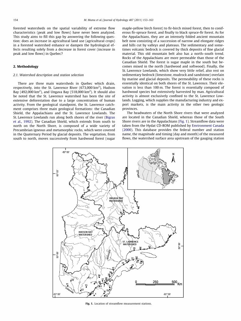
Fig. 1. Location of streamflow

maple-yellow birch forest) to fir-birch mixed forest, then to conif-erous fir-spruce forest, and finally to black spruce-fir forest. As forthe Appalachians, they are an intensely folded ancient mountainbelt now consisting of a succession of narrow and elongate ridgesand hills cut by valleys and plateaus. The sedimentary and some-times volcanic bedrock is covered by thick deposits of fine glacialmaterial. This old mountain belt also has a north–south trend.Rocks of the Appalachians are more permeable than those of theCanadian Shield. The forest is sugar maple in the south but be-comes mixed in the north (hardwood and softwood). Finally, theSt. Lawrence Lowlands, which show very little relief, also rest onsedimentary bedrock (limestone, mudrock and sandstone) overlainby marine and glacial deposits. The permeability of these rocks isessentially identical on both shores of the St. Lawrence. Their ele-vation is less than 100 m. The forest is essentially composed ofhardwood species but extensively harvested by man. Agriculturalactivity is almost exclusively confined to the St. Lawrence Low-lands. Logging, which supplies the manufacturing industry and ex-port markets, is the main activity in the other two geologicprovinces.

The headwaters of the North Shore rivers that were analyzedare located in the Canadian Shield, whereas those of the SouthShore rivers are in the Appalachians (Fig. 1). Streamflow data weretaken from the Hydat CD-ROM published by Environment Canada(2000). This database provides the federal number and stationname, the magnitude and timing (day and month) of the measuredflows, the watershed surface area upstream of the gauging station

measurement stations.

M. Muma et al. / Journal of Hydrology 407 (2011) 153–163 155

and the geographical coordinates of the station (latitude andlongitude). To allow analysis of a large number of stations, thestudy was restricted to the period from 1960 to 1990. Thirty-sixstations were selected for which streamflow data were availableover a minimum of 20 consecutive years. Catchment surface areasfor these stations range from 208 km2 to 3729 km2, with a medianvalue of 1138 km2 (Table 1). Many physiographic features werecalculated over this period, including forest, lake and marshsurface areas for all watersheds, mean slope, stream length, etc.(Belzile et al., 1997; Desforges and Tremblay, 1974). It is worthpointing out that none of the rivers analyzed show a significantchange in the mean or the variance of their flow characteristics(stationary series) over the 1960–1990 interval. This stationaritywas confirmed using the Lombard test, with which the mean andvariance of analyzed series can be tested simultaneously. Further-more, since the study looks at the link between agricultural landcover and the spatial variability of flows, the time interval overwhich flows were measured need not be exactly identical for all36 stations. Finally, the flow data analyzed are not affected bydams or hydroelectric power plants.

The forested land cover, reported as a percentage of the totalsurface area of the watershed, was calculated by subtracting thesurface area of lakes and marshes, farmland, and the urban domain(cities, towns, industrial parks, etc.) from the total surface area ofthe watershed. The surface area covered by lakes and marshes,farmland and the urban domain was first calculated with a digitalplanimeter from 1:250,000 topographic maps (Belzile et al., 1997;Desforges and Tremblay, 1974;). However, unlike data for lake andmarsh surface area, data on the surface area of farmland and theurban domain are not available for the 1960–1990 interval. Some

Table 1List of analyzed rivers.

# Stations ID DA (km2) FC (%) MS (m/km) Years

1 Châteauguay 02OA054 2463 31.0 4.3 312 Nicolet SW 02OD001 544 49.0 2.5 313 Nicolet 02OD003 1540 40.0 1.9 244 Coaticook 02OE022 521 57.0 4.4 315 Beaurivage 02PJ007 707 44.0 4.8 316 Bécancour 02PL005 924 53.9 2.4 237 Bécancour 02PL007 2317 47.0 1.3 208 Matapédia 01BD002 2734 83.6 1.6 219 Kinojévis 02JB013 2575 88.1 0.3 24

10 Dumoine 02KJ003 2111 87.0 0.5 2311 Dumoine 02KJ004 3729 88.0 1.4 2512 Petite Nation 02LD005 1404 81.0 1.2 2213 Maskinongé 02OC002 1023 81.3 5.1 2514 Hall 02OE018 218 84.0 6.9 3115 Eaton 02OE027 642 84.0 5.6 3116 Du Sud 02PH010 824 74.0 6.4 2417 Trois Pistoles 02QA001 966 74.0 4.1 3118 Blanche 02QB005 208 83.0 4.9 2419 Nabisipi 02WA001 2080 86.0 3.4 2620 Harricana 04NA001 3704 72.0 0.3 3121 Nouvelle 01BF001 1138 98.2 7.2 2722 York 01BH002 1015 98.3 5.0 2223 Darmouth 01BH005 630 99.8 6.4 2124 Croche 02NE011 1579 96.0 3.1 2625 Du Loup 02OC004 781 92.0 4.1 2526 Batiscan 02PA007 4400 90.0 1.9 2327 Sainte-Anne 02PB019 1438 93.4 7.9 2528 Montmorency 02PD002 1100 96.0 8.5 2629 Du Gouffre 02PE009 862 91.0 10.1 2330 Malbaie 02PF001 1631 96.0 6.0 2331 Rimouski 02QA002 1586 92.0 3.7 2832 Matane 02QB001 1647 94.0 4.6 3133 Cap-Chat 02QB011 722 97.8 5.1 2434 Madeleine 02QC001 1217 99.0 3.4 3135 des Rapides 02UB001 554 91.0 13.6 2336 Au Tonnerre 02VA001 684 93.0 5.5 25

DA = drainage area; FC = forest cover; MS = mean slope.

data postdating that interval are, however, available for some ofthe watersheds (Grenier et al., 2006; Lavoie et al., 2006). These dataare presented in Table 2, which shows that all watersheds with for-est cover representing less than 60% of the total surface area arecharacterized by relatively extensive agricultural crops. In contrast,urban surface area varies little from one watershed to the next. Inlight of these data, it may be concluded that areas not covered byforest are mostly used for agriculture.

Due to the lack of data on agricultural land cover for manywatersheds, streamflow was compared with forest cover. Hence,this is an indirect analysis of the relationship between streamflowand agricultural land cover.

Streams were subdivided into three classes as a function of for-est land cover (Table 1):

– Class A includes 6 streams for which forest cover accounts forless than 60% of the watershed area.

– Class B includes 13 streams for which forest cover accounts for60–90% of the watershed area.

– Class C includes 16 streams for which forest cover accountsfrom more than 90% of the watershed area.

This subdivision scheme made it easier to highlight the effect ofthe change of forest cover into agricultural land cover and wassuch that the number of streams in each class lent itself to statis-tical analysis.

The average slope of the watershed was calculated according toBenson’s method, commonly known as the ‘‘85-10’’ method. Thistakes the average slope of the central part of the main section,measured between points located at distances of 0.85 L and0.10 L on the longitudinal axis of the watercourse from the pointfarthest from the mouth, with L corresponding to the total lengthof the main watercourse (Desforges and Tremblay, 1974).

Studies on the hydrological regionalization of flows in Quebechave shown that the spatial variability of annual, seasonal,monthly and daily streamflow mostly depends on watershed sur-face area (e.g. Anctil et al., 1998; Assani et al., 2005, 2006, 2007; La-joie et al., 2007; Ribeiro-Corréa et al., 1995). The effect of otherfactors such as stream length, drainage density, average slope ofthe watershed, and so on is very limited. For this reason, these fac-tors were not taken into account. As for weather data, since it wasnot possible to obtain temperature or precipitation data for all ofthe watersheds, data taken from a few regional studies focusedon these climate variables were used (e.g. Assani et al., 2006a, inpress; Khaliq et al., 2007; Lacroix and Boivin, 1992).

2.2. Definition of flow characteristics, hydrologic series compositionand periods of summer season

From an ecological standpoint, Ritcher et al. (1996) and Poffet al. (1997) showed that streamflow may be described in termsof five fundamental characteristics: magnitude, frequency, vari-ability (rate of change), duration and timing of flow. These charac-teristics define the ‘‘natural flow regime’’ of a stream, a concept

Table 2Comparison of percent of forest covert area (FC), agricultural (farmland) area (AA) andurban surface area (UA) in some watersheds.

FC (%) AA (%) UA (%)

Châteaugay 31.0 33.9 0.4Nicolet 40.0 42.9 1.7Coaticook 57.0 24.9 1.0Becancour (924) 53.9 28.5 2.6De la Petite Nation 81.0 0.31 0Maskinongé 81.3 10.2 2.1Du Loup 92.0 7.4 3.1


which is becoming widely used in aquatic ecology as well as inhydrology. According to these authors, each characteristic playsan essential role in the aquatic ecosystem function. For the firsttime, they defined the ecological impacts associated with each fun-damental flow characteristic in natural streams as well as in thoseaffected by human activity. Assani et al. (2006b, 2010) introducedtwo important concepts that make it easier to apply the naturalflow regime concept in hydrology: the flow ‘‘characteristic’’ andthe ‘‘hydrologic variable’’. According to these authors, a flow char-acteristic is an intrinsic property of fluvial flow, whereas a hydro-logic variable is a statistical variable which allows the definitionof a flow characteristic. For instance, the magnitude is an intrinsicproperty of flow and the arithmetic mean of magnitude values is ahydrologic variable. Thus, a flow characteristic may be defined bymany hydrologic variables. In the case of magnitude, aside fromthe arithmetic mean, it may also be defined using a percentile va-lue or an extreme value. Incidentally, according to Assani et al.(2006a,b), the number of definable characteristics depends on thehydrologic series. For a seasonal series (consisting exclusively ofthe highest daily flow values measured each year during a givenseason), only three characteristics may be defined, namely magni-tude, frequency and its timing. Definition of the other characteris-tics of extreme flows requires the analysis of a partial seasonalseries, that is a series consisting of flow values at or above a giventhreshold value. Taking the foregoing into account, the hydrologicseries studied were established according to the followingprocedure:

(a) As a first step, the summer season (May–October) wasdivided in three distinct periods according to the mainindustrial agricultural activities (mostly related to graincrops) carried out in Quebec and surface texture. Each periodis roughly two months long (Table 3). The reason for thissubdivision is that the evapotranspiration, runoff and infil-tration conditions that affect peak and low flows changeduring the summer season as a result of changes in culti-

Table 4aCharacteristics and hydrologic variables of daily maximum flows.

Series type Characteristics Hydrologicvariable

Method

Seasonal maximumseries

Magnitude–frequency QM Arithmeduring e

QMe Medianduring e

P90M 90th perduring e

P10M 10th perduring e

Timing TQM Arithme

Partial series Magnitude–frequency QMM Arithmeduring e

Duration of magnitude DQMM ArithmeTiming of magnitude TQMM ArithmeVariability ofmagnitude

CVQMM Arithmeflows P

Qx is the lowest value of the highest daily maximum flows (seasonally daily maximum flo

Table 3Subdivision of the summer season into three periods as a function of the mainagricultural activities (industrial crops) and surface texture.

Period Month Main agricultural activities and surface texture

I May–June Sowing period. Soil protection by crops is verylimited

II July–August Growing period. Soil protection by crops is goodIII September–

OctoberHarvesting and plowing period. Soil protection bycrops is limited

vated plant over and surface texture in crop areas, amongothers. Even in forested areas, deciduous species foliage den-sity changes from month to month, which affects transpira-tion and rainfall interception by trees. The rationale forchoosing the period from May to October is that in someareas of Quebec, the ground remains completely coveredby snow until April. In addition, previous studies haveshown that the effect of plant cover on the temporal vari-ability of flows is strongest during summer (Caissie et al.,2002; Lavigne et al., 2004).

(b) The second step consisted in selecting, for each of the threesummer periods defined in the first step and for each station(stream), the highest daily maximum flow (seasonally dailymaximum flow) and the lowest daily minimum flow mea-sured (seasonally daily minimum flow) each year duringthe 1960–1990 period. Thus, a series of daily maximumflows and a series of daily minimum flows were establishedfor each station and each of the three summer periods.Finally, for each station and each period, the arithmeticmeans, the median, the percentile and the timing mean ofthe seasonally daily maximum flows (QM, QMe, P90M,P10M and TQM) and the seasonally daily minimum flows(Qm, Qme, P90m, P10m and TQm) were calculated overthe 1960–1990 period.

To make up the partial seasonal series, the following steps weretaken, following the approach described in Assani et al. (2010):

(c) The third step consisted in determining, for each station andeach summer period, the lowest value (Qx) of daily maxi-mum flows and the highest value (Qy) of daily minimumflows (the series obtained through step 2).

(d) The fourth step consisted, for each of the summer periodsand each year, in selecting all values of daily flow greaterthan Qx (for daily maximum flows) and smaller than Qy(for daily minimum flows). Thus, for each station and eachsummer period, two partial series were obtained with Qx(highest maximum flow partial series) and Qy (lowest min-imum flows partial series) as thresholds, for daily maximumand minimum flows, respectively.

(e) The last step was to calculate the hydrologic variables thatdefine flow characteristics for the series obtained in thefourth step. For magnitude–frequency (QMM), the arithme-tic mean of the flow values equal to or greater than Qx ata given station over the 1960–1990 period was calculatedfor each of the three summer periods. For each year, the

of calculation

tic mean of highest daily maximum flows measured over the 1960–1990 periodach of the three summer periodsvalue of highest daily maximum flows measured over the 1960–1990 periodach of the three summer periodscentile of highest daily maximum flows measured over the 1960–1990 periodach of the three summer periodscentile of highest daily maximum flows measured over the 1960–1990 periodach of the three summer periodstic mean of the dates (in Julian days) of highest daily maximum flows

tic mean of highest daily minimum flows measured over the 1960–1990 periodach of the three summer periodstic mean of the number of days during which daily maximum flows P Qxtic mean of the dates (in Julian days) during which daily maximum flows P Qxtic mean of the coefficients of variation of the magnitude of daily maximumQx

ws) measured over the 1960–1990 period during each of the three summer periods.

Table 4bCharacteristics and hydrologic variables of daily minimum flows.

Series type Characteristics Hydrologicvariable

Method of calculation

Seasonal maximum series Magnitude–frequency Qm Arithmetic mean of lowest daily maximum flows measured over the 1960–1990period during each of the three summer periods

Qme Median value of lowest daily maximum flows measured over the 1960–1990 periodduring each of the three summer periods

P90m 90th percentile of lowest daily maximum flows measured over the 1960–1990period during each of the three summer periods

P10m 10th percentile of lowest daily maximum flows measured over the 1960–1990period during each of the three summer periods

Timing TQm Arithmetic mean of the dates (in Julian days) of lowest daily minimum flows

Partial series Magnitude–frequency Qmm Arithmetic mean of lowest daily minimum flows measured over the 1960–1990period during each of the three summer periods

Duration of magnitude DQmm Arithmetic mean of the number of days during which daily minimum flows 6 QyTiming of magnitude TQmm Arithmetic mean of the dates (in Julian days) during which daily minimum

flows 6 QyVariability of magnitude CVQmm Arithmetic mean of the coefficients of variation of the magnitude of daily minimum

flows 6 Qy

Qy is the highest value of the lowest daily minimum flows (seasonally daily minimum flows) measured over the 1960–1990 period during each of the three summer periods.


duration of these floods is equal to the total number of daysduring which Qx was reached or exceeded. Then, for eachstation, the mean duration (DQMM) of the floods over theperiod from 1960 to 1990 was calculated for each of thethree summer periods. As for timing, the arithmetic meanof the dates (in Julian days) of flows (TQMM) equal to orgreater than Qx was calculated. Finally, the variability ofthe magnitude (CVQMM) was calculated using the coeffi-cient of variation, which is the ratio of the arithmetic meanof flows P Qx and its standard deviation. The same approachwas applied to flows equal to or smaller than Qy to deter-mine the flow characteristics of low flows. Finally, for eachstation, the arithmetic mean of each flow characteristic(for maximum and minimum flows) was calculated overthe 1960–1990 period. For magnitude–frequency, the onlycharacteristic defined for both types of series, ‘‘daily meanmaximum flows’’ (QMM) and ‘‘daily mean minimum flows’’(Qmm) are defined as the mean values of flow magnitude–frequency calculated for both partial series. All the hydro-logic variables analyzed are defined in Table 4a (daily max-imum flows) Table 4b (daily minimum flows).

As for the frequency of extreme flows, it can be defined in twoways:

– In the same units as magnitude, that is in m3/s. For instance, aflow value corresponding to a given recurrence interval or agiven percentile on a flow frequency distribution curve can bedetermined. The magnitude of this flow, in m3/s, is used forthe purpose of analysis rather than the recurrence interval orthe percentile value. In such cases, the frequency and magni-tude are inextricably linked and cannot be distinguished. In fact,in the course of analyzing the spatial variability of flow (flowdata collected from many stream gauging stations), Assaniet al. (2006a, 2007) showed that all hydrological variableswhich define the same type of measurement (location, disper-sion, skewness, etc.) for a given characteristic are strongly cor-related, and therefore redundant. To avoid such redundancy, asingle one of these variables may therefore be used to definecompletely the magnitude–frequency characteristic.

– As the number of times a flow of a given magnitude is reachedor exceeded during a given time interval (exceedance frequencyor probability). In such cases, frequency is no longer expressedin the same units as magnitude. The two characteristics are nolonger inextricably linked and the hydrological variables which

define them are only weakly or moderately correlated (seeexamples in Assani et al., 2010; Fortier et al., in press).

For this study, frequency was defined only for seasonal series(second step), that is, in the same units as magnitude. Four vari-ables were used to define the two characteristics (magnitude–fre-quency): the mean (QM and Qm), the median (QMe, Qme), and thevalues of flow (magnitude) corresponding to the 10th (Q10M andQ10m) and 90th (Q90M and Q90m) percentiles (Table 2). Becauseof the redundancy, it was not necessary to calculate the four vari-ables for the partial series. All characteristics were defined by a sin-gle hydrological variable, namely the arithmetic mean (Table 2).The choice of this hydrologic variable is based on the fact that itwas subsequently used in the analysis of covariance, this methodbeing only applicable to the mean values of data series.

2.3. Statistical analysis

Statistical analysis was carried out in two steps.

– In the first step, all hydrological variables, as defined in Sec-tion 2.3 above, were correlated to percent forest cover in water-sheds. It should be recalled that data on agricultural land coverwere not available for all analyzed watersheds. This correlationwas analyzed using the canonical correlation analysis (CANCO-RAN) method. Then, this multivariate statistic was used to cal-culate the relationship between independent variables(Drainage area, forested surface area, surface area of lakes andmarshes) and dependent variables (hydrologic variables of dailyextreme maximum and minimum flows). This method was cho-sen because it allows calculation of the correlation betweenvariables of two different groups, on one hand, and betweenvariables of the same group, on the other hand, while maximiz-ing correlation coefficients. As such, it provides the general the-oretical framework for factorial discriminant analysis,multivariate regression and correspondence analysis tech-niques (Ouarda et al., 2001). Canonical correlation analysis isperformed first by extracting the canonical factors from bothgroups of variables. Canonical factors derived from the indepen-dent variables group are labeled Vp and those derived from thedependent variables group (hydrologic variables) are labeledWq. The point of the analysis is to maximize the correlationcoefficients between the canonical factors (V and W) for bothgroups. Note that Vp and Vq are linear combinations oforiginally independent and dependent variables. Thus, the


correlation coefficients are calculated at two levels. First, corre-lation coefficients are calculated between the canonical factorsVp and Wq. These coefficients are called canonical correlationcoefficients. Second, simple correlation coefficients betweencanonical factors Vp and the original independent variables onthe one hand, and between canonical factors Wq and the origi-nal dependent variables, on the other hand, are calculated.These simple correlation coefficients are called structure coeffi-cients. The mathematical details of the canonical correlationanalysis are described in Afifi and Clark (1996), among others.

– As canonical correlation analysis does not allow determinationof the nature of the link between forest land cover (or, indi-rectly, agricultural land cover) and the hydrologic variables,covariance analysis (ANCOVA) (Dagnelie, 1986) was used inthe second step. This consisted in comparing extreme flow val-ues (quantitative dependent variable) measured at differentstations as a function of catchment surface area (quantitativeindependent variable) and percentage (the three classes) of for-est cover (qualitative independent variable), as well as theeffects of the interaction of these two independent variables.It is worth recalling that the analysis of covariance approacharises from the analysis of variance applied to a classificationcriterion and from simple linear regression. In general, it canbe used to model simultaneously the effects of a multi-classqualitative variable (classification criterion) and a quantitativevariable on a dependant quantitative variable. Alila et al.(2009) have recently challenged the use of this method inpaired watershed studies because, as already pointed out, thesestudies focus on time series of measured flows at a single sta-tion, whereas the method is designed to compare mean valuesof flow measured at various stations (spatial variability). Giventhat the present study is concerned with the spatial variabilityof flow, the use of the analysis of covariance method is statisti-cally sound.

3. Results

3.1. Analysis of the relationship between forest cover and hydrologicvariables using the CANCORAN method

For daily minimum flows (Table 5), values of the first canonicalcorrelation coefficient are nearly identical for each of the threesummer periods. All three are greater than 0.96, which indicates

Table 5Comparison of the canonical correlation (CC). coefficient values for the three summer per

Period I Period II

CC F p > F CC

CC1 0.98044 12.42 <0.0001 0.98830CC2 0.63780 1.98 0.0531 0.54167CC3 0.28258 0.63 0.6456 0.37788

CC = canonical correlation coefficient; F = value calculated with the Fisher–Snedecor tesStatistically significant p values are shown in bold.

Table 6aCanonical correlations between independent variables and canonical factors (V). Daily min

Period I Period II

V1 V2 V3 V1

DA 0.924 �0.033 �0.381 0.918FC 0.959 0.2490 �0.137 0.965LM 0.850 �0.484 0.201 0.834EV (%) 83.1 9.9 6.9 82.3

DA = drainage area, FC = forested surface area; LM = surface area of lakes and marshes.EV = explained variance. Highest statistically significant correlation coefficients are show

a strong link between the two groups of variables. The first twocanonical correlation coefficients are statistically significant forall the three summer periods. Analysis of the correlation betweenthe canonical factors and the independent variables (drainage area,forested cover, surface area of lakes and marshes) shows that theindependent variables are all strongly correlated to the first canon-ical factor (V1) for all three periods (Table 6a). Its explained vari-ance is greater than 70%. Notably, forested cover shows thestrongest correlation with the first canonical factor. As for hydro-logic variables, all those variables (Qm, Qme, QP90m, QP10m andQmm) which define the magnitude–frequency characteristic ofdaily minimum flows show a strong correlation with the firstcanonical factor (W1), whose explained variance is greater than50% for all three periods (Table 6b), these five variables beingstrongly correlated. As previously shown by Assani et al. (2006a,2007), this result confirms the fact that all hydrological variableswhich define a given flow characteristic for a seasonal or partialseries, namely the magnitude–frequency characteristic, arestrongly correlated. In other words, there is a redundancy. To avoidsuch redundancy for the partial series, a single hydrological vari-able, namely the mean of the series, was used to define all flowcharacteristics. Since V1 and W1 are correlated, the magnitude–frequency of minimum flows is the only characteristic which issignificantly correlated to forest cover area during all threesummer periods. This correlation is positive.

As for daily maximum flows, although CANCORAN results(Tables 7 and 8a and 8b) are similar to those obtained for dailyminimum flows, there are some notable differences:

– The values of the first canonical correlation coefficient are rela-tively smaller for daily maximum flows than for daily minimumflows. All are lower than 0.96. This means that the link betweenthe two groups of variables is weaker for maximum flows thanfor minimum flows.

– The coefficient of variation of the magnitude becomes signifi-cantly correlated to forest surface area during the third summerperiod. This correlation is negative.

3.2. Quantification of changing a forested land use into an agriculturalland use on extreme flow characteristics using ANCOVA method

It should be noted that although CANCORAN can be used tohighlight the presence of a significant linear relationship between

iods. Daily minimum flows.

Period III

F p > F CC F p > F

9.32 <0.0001 0.96288 9.64 <0.00011.60 0.1319 0.63322 2.43 0.01731.21 0.3288 0.43482 1.69 0.1792

t.

imum flows.

Period III

V2 V3 V1 V2 V3

0.180 0.354 0.926 �0.255 0.279�0.160 0.205 0.990 �0.127 �0.066

0.430 �0.344 0.761 0.447 0.4708.1 9.6 80.5 9.4 10.1

n in bold.

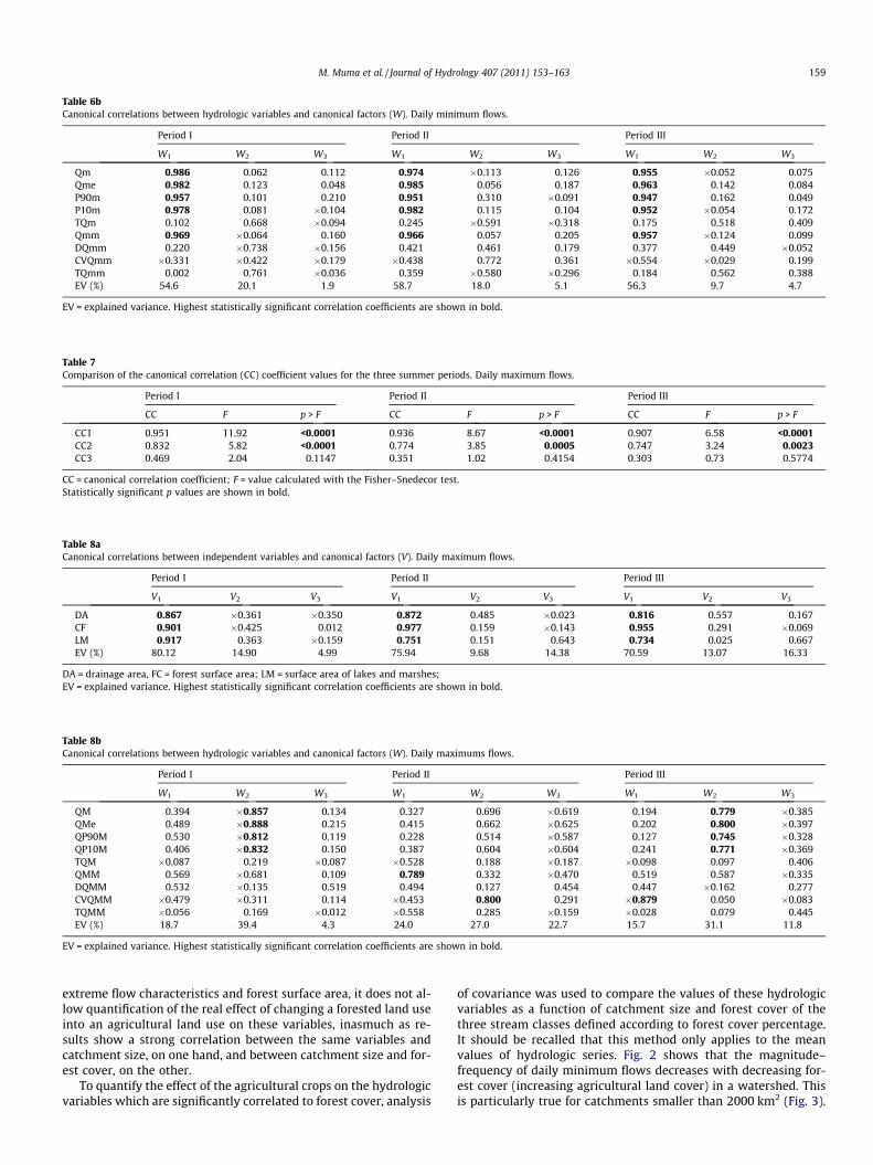
Table 6bCanonical correlations between hydrologic variables and canonical factors (W). Daily minimum flows.

Period I Period II Period III

W1 W2 W3 W1 W2 W3 W1 W2 W3

Qm 0.986 0.062 0.112 0.974 �0.113 0.126 0.955 �0.052 0.075Qme 0.982 0.123 0.048 0.985 0.056 0.187 0.963 0.142 0.084P90m 0.957 0.101 0.210 0.951 0.310 �0.091 0.947 0.162 0.049P10m 0.978 0.081 �0.104 0.982 0.115 0.104 0.952 �0.054 0.172TQm 0.102 0.668 �0.094 0.245 �0.591 �0.318 0.175 0.518 0.409Qmm 0.969 �0.064 0.160 0.966 0.057 0.205 0.957 �0.124 0.099DQmm 0.220 �0.738 �0.156 0.421 0.461 0.179 0.377 0.449 �0.052CVQmm �0.331 �0.422 �0.179 �0.438 0.772 0.361 �0.554 �0.029 0.199TQmm 0.002 0.761 �0.036 0.359 �0.580 �0.296 0.184 0.562 0.388EV (%) 54.6 20.1 1.9 58.7 18.0 5.1 56.3 9.7 4.7

EV = explained variance. Highest statistically significant correlation coefficients are shown in bold.

Table 7Comparison of the canonical correlation (CC) coefficient values for the three summer periods. Daily maximum flows.


CC F p > F CC F p > F CC F p > F

CC1 0.951 11.92 <0.0001 0.936 8.67 <0.0001 0.907 6.58 <0.0001CC2 0.832 5.82 <0.0001 0.774 3.85 0.0005 0.747 3.24 0.0023CC3 0.469 2.04 0.1147 0.351 1.02 0.4154 0.303 0.73 0.5774

CC = canonical correlation coefficient; F = value calculated with the Fisher–Snedecor test.Statistically significant p values are shown in bold.

Table 8aCanonical correlations between independent variables and canonical factors (V). Daily maximum flows.


V1 V2 V3 V1 V2 V3 V1 V2 V3

DA 0.867 �0.361 �0.350 0.872 0.485 �0.023 0.816 0.557 0.167CF 0.901 �0.425 0.012 0.977 0.159 �0.143 0.955 0.291 �0.069LM 0.917 0.363 �0.159 0.751 0.151 0.643 0.734 0.025 0.667EV (%) 80.12 14.90 4.99 75.94 9.68 14.38 70.59 13.07 16.33

DA = drainage area, FC = forest surface area; LM = surface area of lakes and marshes;EV = explained variance. Highest statistically significant correlation coefficients are shown in bold.

Table 8bCanonical correlations between hydrologic variables and canonical factors (W). Daily maximums flows.


W1 W2 W3 W1 W2 W3 W1 W2 W3

QM 0.394 �0.857 0.134 0.327 0.696 �0.619 0.194 0.779 �0.385QMe 0.489 �0.888 0.215 0.415 0.662 �0.625 0.202 0.800 �0.397QP90M 0.530 �0.812 0.119 0.228 0.514 �0.587 0.127 0.745 �0.328QP10M 0.406 �0.832 0.150 0.387 0.604 �0.604 0.241 0.771 �0.369TQM �0.087 0.219 �0.087 �0.528 0.188 �0.187 �0.098 0.097 0.406QMM 0.569 �0.681 0.109 0.789 0.332 �0.470 0.519 0.587 �0.335DQMM 0.532 �0.135 0.519 0.494 0.127 0.454 0.447 �0.162 0.277CVQMM �0.479 �0.311 0.114 �0.453 0.800 0.291 �0.879 0.050 �0.083TQMM �0.056 0.169 �0.012 �0.558 0.285 �0.159 �0.028 0.079 0.445EV (%) 18.7 39.4 4.3 24.0 27.0 22.7 15.7 31.1 11.8

EV = explained variance. Highest statistically significant correlation coefficients are shown in bold.


extreme flow characteristics and forest surface area, it does not al-low quantification of the real effect of changing a forested land useinto an agricultural land use on these variables, inasmuch as re-sults show a strong correlation between the same variables andcatchment size, on one hand, and between catchment size and for-est cover, on the other.

To quantify the effect of the agricultural crops on the hydrologicvariables which are significantly correlated to forest cover, analysis

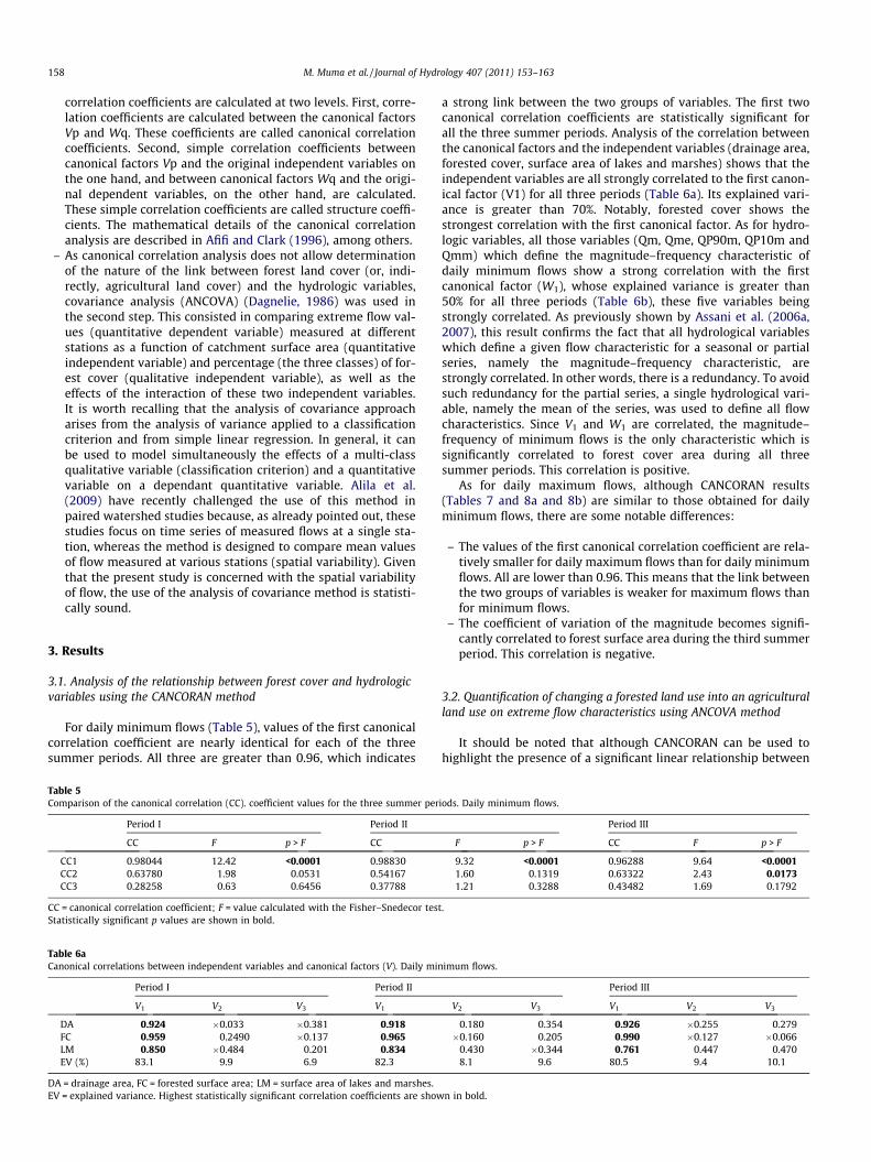
of covariance was used to compare the values of these hydrologicvariables as a function of catchment size and forest cover of thethree stream classes defined according to forest cover percentage.It should be recalled that this method only applies to the meanvalues of hydrologic series. Fig. 2 shows that the magnitude–frequency of daily minimum flows decreases with decreasing for-est cover (increasing agricultural land cover) in a watershed. Thisis particularly true for catchments smaller than 2000 km2 (Fig. 3).

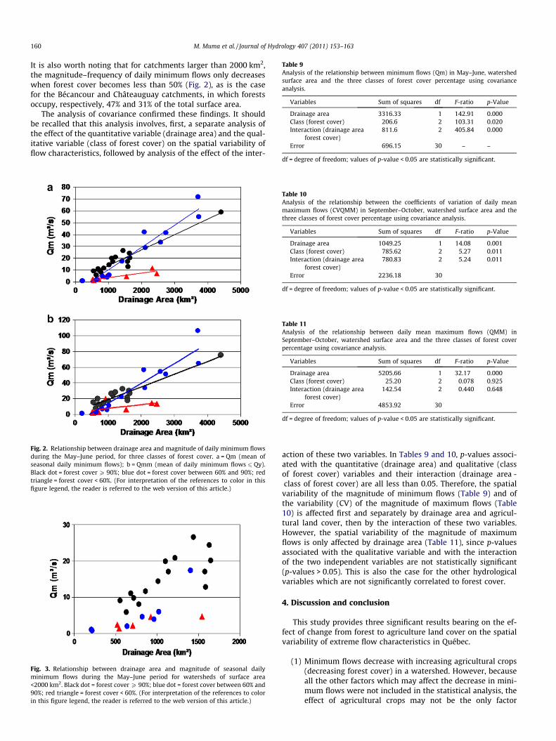
Table 9Analysis of the relationship between minimum flows (Qm) in May–June, watershedsurface area and the three classes of forest cover percentage using covarianceanalysis.

Variables Sum of squares df F-ratio p-Value

Drainage area 3316.33 1 142.91 0.000Class (forest cover) 206.6 2 103.31 0.020Interaction (drainage area� forest cover)

811.6 2 405.84 0.000

Error 696.15 30 – –


It is also worth noting that for catchments larger than 2000 km2,the magnitude–frequency of daily minimum flows only decreaseswhen forest cover becomes less than 50% (Fig. 2), as is the casefor the Bécancour and Châteauguay catchments, in which forestsoccupy, respectively, 47% and 31% of the total surface area.

The analysis of covariance confirmed these findings. It shouldbe recalled that this analysis involves, first, a separate analysis ofthe effect of the quantitative variable (drainage area) and the qual-itative variable (class of forest cover) on the spatial variability offlow characteristics, followed by analysis of the effect of the inter-

Fig. 2. Relationship between drainage area and magnitude of daily minimum flowsduring the May–June period, for three classes of forest cover. a = Qm (mean ofseasonal daily minimum flows); b = Qmm (mean of daily minimum flows 6 Qy).Black dot = forest cover P 90%; blue dot = forest cover between 60% and 90%; redtriangle = forest cover < 60%. (For interpretation of the references to color in thisfigure legend, the reader is referred to the web version of this article.)

Fig. 3. Relationship between drainage area and magnitude of seasonal dailyminimum flows during the May–June period for watersheds of surface area<2000 km2. Black dot = forest cover P 90%; blue dot = forest cover between 60% and90%; red triangle = forest cover < 60%. (For interpretation of the references to colorin this figure legend, the reader is referred to the web version of this article.)

df = degree of freedom; values of p-value < 0.05 are statistically significant.

Table 10Analysis of the relationship between the coefficients of variation of daily meanmaximum flows (CVQMM) in September–October, watershed surface area and thethree classes of forest cover percentage using covariance analysis.



780.83 2 5.24 0.011

Error 2236.18 30


Table 11Analysis of the relationship between daily mean maximum flows (QMM) inSeptember–October, watershed surface area and the three classes of forest coverpercentage using covariance analysis.



142.54 2 0.440 0.648

Error 4853.92 30


action of these two variables. In Tables 9 and 10, p-values associ-ated with the quantitative (drainage area) and qualitative (classof forest cover) variables and their interaction (drainage area -class of forest cover) are all less than 0.05. Therefore, the spatialvariability of the magnitude of minimum flows (Table 9) and ofthe variability (CV) of the magnitude of maximum flows (Table10) is affected first and separately by drainage area and agricul-tural land cover, then by the interaction of these two variables.However, the spatial variability of the magnitude of maximumflows is only affected by drainage area (Table 11), since p-valuesassociated with the qualitative variable and with the interactionof the two independent variables are not statistically significant(p-values > 0.05). This is also the case for the other hydrologicalvariables which are not significantly correlated to forest cover.

4. Discussion and conclusion

This study provides three significant results bearing on the ef-fect of change from forest to agriculture land cover on the spatialvariability of extreme flow characteristics in Québec.

(1) Minimum flows decrease with increasing agricultural crops(decreasing forest cover) in a watershed. However, becauseall the other factors which may affect the decrease in mini-mum flows were not included in the statistical analysis, theeffect of agricultural crops may not be the only factor

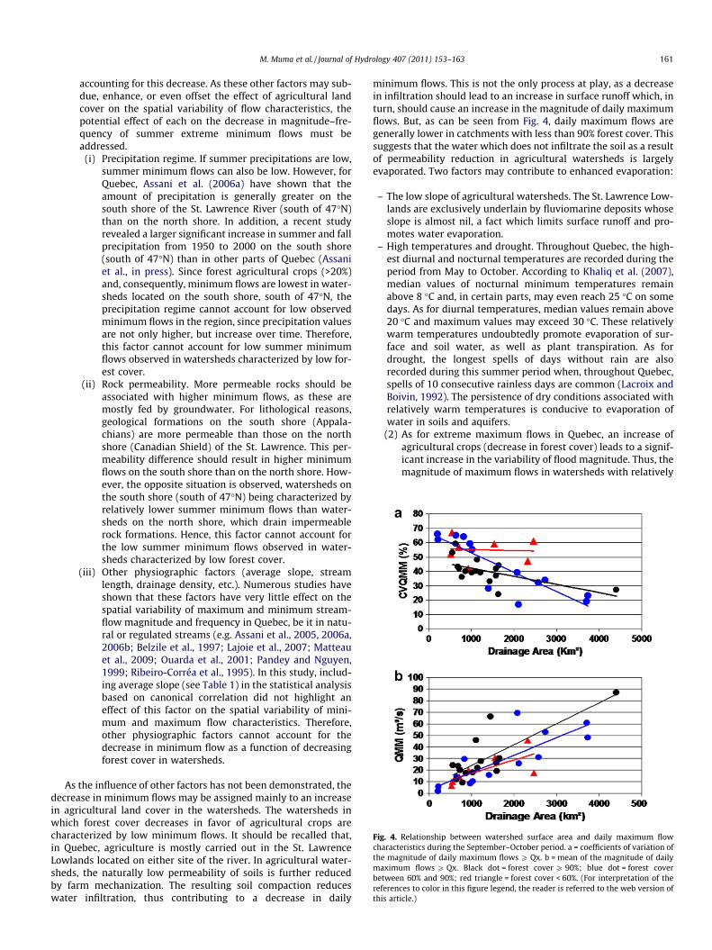
Fig. 4. Relationship between watershed surface area and daily maximum flowcharacteristics during the September–October period. a = coefficients of variation ofthe magnitude of daily maximum flows P Qx. b = mean of the magnitude of dailymaximum flows P Qx. Black dot = forest cover P 90%; blue dot = forest coverbetween 60% and 90%; red triangle = forest cover < 60%. (For interpretation of thereferences to color in this figure legend, the reader is referred to the web version ofthis article.)


accounting for this decrease. As these other factors may sub-due, enhance, or even offset the effect of agricultural landcover on the spatial variability of flow characteristics, thepotential effect of each on the decrease in magnitude–fre-quency of summer extreme minimum flows must beaddressed.

(i) Precipitation regime. If summer precipitations are low,summer minimum flows can also be low. However, forQuebec, Assani et al. (2006a) have shown that theamount of precipitation is generally greater on thesouth shore of the St. Lawrence River (south of 47�N)than on the north shore. In addition, a recent studyrevealed a larger significant increase in summer and fallprecipitation from 1950 to 2000 on the south shore(south of 47�N) than in other parts of Quebec (Assaniet al., in press). Since forest agricultural crops (>20%)and, consequently, minimum flows are lowest in water-sheds located on the south shore, south of 47�N, theprecipitation regime cannot account for low observedminimum flows in the region, since precipitation valuesare not only higher, but increase over time. Therefore,this factor cannot account for low summer minimumflows observed in watersheds characterized by low for-est cover.

(ii) Rock permeability. More permeable rocks should beassociated with higher minimum flows, as these aremostly fed by groundwater. For lithological reasons,geological formations on the south shore (Appala-chians) are more permeable than those on the northshore (Canadian Shield) of the St. Lawrence. This per-meability difference should result in higher minimumflows on the south shore than on the north shore. How-ever, the opposite situation is observed, watersheds onthe south shore (south of 47�N) being characterized byrelatively lower summer minimum flows than water-sheds on the north shore, which drain impermeablerock formations. Hence, this factor cannot account forthe low summer minimum flows observed in water-sheds characterized by low forest cover.

(iii) Other physiographic factors (average slope, streamlength, drainage density, etc.). Numerous studies haveshown that these factors have very little effect on thespatial variability of maximum and minimum stream-flow magnitude and frequency in Quebec, be it in natu-ral or regulated streams (e.g. Assani et al., 2005, 2006a,2006b; Belzile et al., 1997; Lajoie et al., 2007; Matteauet al., 2009; Ouarda et al., 2001; Pandey and Nguyen,1999; Ribeiro-Corréa et al., 1995). In this study, includ-ing average slope (see Table 1) in the statistical analysisbased on canonical correlation did not highlight aneffect of this factor on the spatial variability of mini-mum and maximum flow characteristics. Therefore,other physiographic factors cannot account for thedecrease in minimum flow as a function of decreasingforest cover in watersheds.

As the influence of other factors has not been demonstrated, thedecrease in minimum flows may be assigned mainly to an increasein agricultural land cover in the watersheds. The watersheds inwhich forest cover decreases in favor of agricultural crops arecharacterized by low minimum flows. It should be recalled that,in Quebec, agriculture is mostly carried out in the St. LawrenceLowlands located on either site of the river. In agricultural water-sheds, the naturally low permeability of soils is further reducedby farm mechanization. The resulting soil compaction reduceswater infiltration, thus contributing to a decrease in daily

minimum flows. This is not the only process at play, as a decreasein infiltration should lead to an increase in surface runoff which, inturn, should cause an increase in the magnitude of daily maximumflows. But, as can be seen from Fig. 4, daily maximum flows aregenerally lower in catchments with less than 90% forest cover. Thissuggests that the water which does not infiltrate the soil as a resultof permeability reduction in agricultural watersheds is largelyevaporated. Two factors may contribute to enhanced evaporation:

– The low slope of agricultural watersheds. The St. Lawrence Low-lands are exclusively underlain by fluviomarine deposits whoseslope is almost nil, a fact which limits surface runoff and pro-motes water evaporation.

– High temperatures and drought. Throughout Quebec, the high-est diurnal and nocturnal temperatures are recorded during theperiod from May to October. According to Khaliq et al. (2007),median values of nocturnal minimum temperatures remainabove 8 �C and, in certain parts, may even reach 25 �C on somedays. As for diurnal temperatures, median values remain above20 �C and maximum values may exceed 30 �C. These relativelywarm temperatures undoubtedly promote evaporation of sur-face and soil water, as well as plant transpiration. As fordrought, the longest spells of days without rain are alsorecorded during this summer period when, throughout Quebec,spells of 10 consecutive rainless days are common (Lacroix andBoivin, 1992). The persistence of dry conditions associated withrelatively warm temperatures is conducive to evaporation ofwater in soils and aquifers.(2) As for extreme maximum flows in Quebec, an increase of

agricultural crops (decrease in forest cover) leads to a signif-icant increase in the variability of flood magnitude. Thus, themagnitude of maximum flows in watersheds with relatively


high agricultural surface area is characterized by high coef-ficients of variation. This is particularly true for watershedswith less than 60% forest cover. However, this variabilityincrease is only observed during the last period of thegrowth season. The diversity of factors which cause floodsat that time of year in Quebec, including convective, frontaland cyclonic (the remains of hurricanes and tropical storms)rainfalls, may account for this. The magnitude of floods maytherefore vary considerably according to their cause. Thisdiversity of flood causes is felt in watersheds in which forestcover is reduced. In the case of ‘‘time’’ series of hydrologicalmeasurements (comprised of flow values measured at a sin-gle station over a given time interval), there is a positive lin-ear correlation between arithmetic mean and coefficient ofvariation values. Thus, when the arithmetic mean increasesover time, so does the coefficient of variation. In contrast,for a ‘‘spatial’’ series of hydrological measurements (com-prised of flow values measured at multiple stations of agiven stream or in several streams of different sizes), thereis no link between these two variables. This is because,due to the presence of tributaries, when the arithmetic meanof flow magnitude increases in space as a result of theincreasing size of watersheds, the coefficient of variation offlow magnitude tends to decrease instead. Thus, for a streamwhich is large enough, the mean of the magnitude of flowincreases in the downstream direction, while the variabilityof flow (coefficient of variation) tends to decrease in thatdirection. This well-known observation, dubbed the ‘‘sizeeffect’’, possibly accounts for the lack of a significant correla-tion between the mean of the magnitude of maximum flowsand forest cover surface area, even though forested surfacearea is significantly correlated with the coefficient of varia-tion of the magnitude. Fig. 4 clearly shows a generally posi-tive correlation between watershed surface area and themean of the magnitude of maximum flows, whereas thereis a generally negative correlation between watershed sur-face area and the coefficients of variation, which confirmsthe influence of the ‘‘size effect’’ on the relationship betweenthe mean and the coefficient of variation of the magnitude ofmaximum flows.

(3) Another noteworthy contribution of this study is the defini-tion of the thresholds beyond which a change in the magni-tude–frequency of daily minimum flows is observed inQuebec watersheds. The first threshold is related to the for-ested cover area in a catchment. It has been shown that adecrease in the magnitude–frequency of daily minimumflows is clearly detectable when forest cover area falls below90% (a 10% reduction), for watersheds whose surface area isless than 2000 km2. For larger watersheds, the change isdetectable when forest cover reduction reaches 50%. Theuse of forest cover as a threshold is warranted bythe absence of data on agricultural land cover for all thewatersheds.

Finally, the main conclusion derived from the study is the factthat a shift from forest land use to agricultural land use leads toa complete inversion (offset) of the sole effects of forest cover onminimum flows in Quebec watersheds. Thus, whereas all studieswhich looked at decreasing forest cover in a given watershed inQuebec have shown that this decrease results in an increase inminimum flows, our study shows that, for similar watershed sur-face areas, all watersheds affected by an increase in agriculturalland use at the expense of forest cover are characterized by rela-tively smaller minimum flows. Hence, agricultural land use resultsin a complete inversion of the effects of deforestation on minimumflows. This result is in part akin to that of Poff et al. (2006) for the

United States, as these authors observed that responses to increas-ing agricultural land cover were less pronounced, as minimumflows decreased, near-bankfull increased, and flow variability de-clined. In our study, however, the variability of maximum flow isshown to increase significantly.

Acknowledgements

The authors wish to thank the three reviewers for their veryconstructive comments and suggestions, which have lead to signif-icant improvements to the form and content of this paper. Thisstudy was made possible by an NSERC grant to the second author.

References

Afifi, A.A., Clark, V., 1996. Computer-aided Multivariate Analysis, third ed. Chapmanand Hall, New York.

Alila, Y., Kuras, P.K., Schnorbus, M., Hudson, R., 2009. Forests and floods: a newparadigm sheds light on age-old controversies. Water Resour. Res. 45, W08416,doi:10.1029/2008WR007207.

Alila, Y., Hudson, R., Kuras, P.K., Schnorbus, M., Rasouli, K., 2010. Reply to commentby Jack Lewis et al. on Forests and floods: a new paradigm sheds light on age-old controversies. Water Resour. Res. 46, W05802, doi:10.1029/2009WR009028.

Andréassian, V., 2004a. Waters and forests: from historical controversy to scientificdebate. J. Hydrol. 291, 1–27.

Assani, A.A., Gravel, E., Buffin-Bélanger, T., Roy, A.G., 2005. Impacts des barrages surles caractéristiques des débits annuels minimums en fonction des régimeshydrologiques artificialisés au Québec (Canada). Rev. Sci. de l’Eau 18, 103–127.

Assani, A.A., Stichelbout, É., Roy, A.G., Petit, F., 2006a. Comparison of impacts ofdams on the annual maximum flow characteristics in three regulatedhydrologic regimes in Québec (Canada). Hydrol. Process. 20, 3485–3501.

Assani, A.A., Tardif, S., Lajoie, F., 2006b. Statistical analysis of factors affecting thespatial variability of annual minimum flow characteristics in a cold temperatecontinental region (southern Québec, Canada). J. Hydrol., 328: 753–763.

Assani, A.A., Lajoie, F., Laliberté, C., 2007. Impacts des barrages sur lescaractéristiques des débits moyens annuels en fonction du mode de gestionet de la taille des bassins versants au Québec. Rev. Sci. de l’Eau 20, 127–146.

Assani, A.A., Quessy, J.F., Mesfioui, M., Matteau, M., 2010. An example of application:the ecological «natural flow regime» paradigm in hydroclimatology. Adv. WaterResour. 33, 537–545.

Assani, A.A., Landry, R., Laurencelle, M., in press. Comparison of inter-annualvariability modes and trends of seasonal precipitation and streamflow inSouthern Quebec (Canada). Rivers Res. Appl., doi: 10.1002/rra.1544.

Belzile, L., Bérubé, P., Hoang, V.D., Leclerc, M., 1997. Méthode écohydrologique dedétermination des débits réservés pour la protection des habitats du poissondans les rivières du Québec. Rapport présenté par l’INRS-Eau et le Groupe-conseil Génivar inc. au ministère de l’Environnement et de la Faune et à Pêcheset Océans Canada. 83p + 8 annexes.

Bigras, P., Farrar, C., Bernier, M., Boisvin, F., D’Auteuil, C., 1992. Le Québec au naturel.Les Publications du Québec, Québec.

Blöschl, G., Ardoin-Bardin, S., Bonell, M., Dorninger, M., Goodrich, D., Gutknecht, D.,Matamoros, D., Merz, B., Shand, P., Szolgay, J., 2007. At what scales do climatevariability and land cover change impact on flooding and low flows. Hydrol.Process. 21, 1241–1247.

Caissie, D., Jolicoeur, S., Bouchard, M., Poncet, E., 2002. Comparison of streamflowbetween pre and post timber harvesting in Catamaran Brook (Canada). J.Hydrol. 258, 232–248.

Consandey, C., Andréassian, V., Martin, C., Didon-Lescot, J.F., Lavabre, J., Folton, N.,Mathys, N., Richard, D., 2005. The hydrological impact of the mediterraneanforest: a review of French research. J. Hydrol. 301, 235–249.

Dagnelie, P., 1986. Théorie et méthodes statistiques. Applications agronomiques,vol. 2. Les presses agronomiques de Gembloux, Gembloux, Belgique, p. 463.

Desforges, P., Tremblay, R., 1974. Analyse de la fréquence des crues pour le Québec.Direction générale des eaux, Ministère des Richesses Naturelles, Rapport H.P.-33.

Environment Canada, 2000. Hydat CD-ROM: Données sur les eaux de surface et lessédiments jusqu’en 1998.

Fortier, C, Assani, A.A., Mhamed, M., Roy, A.G., in press. Comparison of theinterannual and interdecadal variability of heavy flood characteristics upstreamand downstream from dams in inversed hydrologic regime: case study ofMatawin River (Québec, Canada). River Res. Appl., doi: 10.1002/rra.1423.

Grenier, M., Campeau, S., Lavoie, I., Park, Y.-S., Lek, S., 2006. Diatom referencecommunities in Québec (Canada) streams based on Kohonen self-organizingmaps and multivariate analyses. Can. J. Fish. Aquat. Sci. 63, 2087–2106.

Hornbeck, J.W., Pierce, R.S., Federer, C.A., 1970. Streamflow changes after forestclearing in New England. Water Res. Res. 6, 1124–1132.

Hornbeck, J.W., Adams, M.B., Corbett, E.S., Verry, E.S., Lynch, J.A., 1993. Long-termimpacts of forest treatments on water yield: a summary for northeastern USA. J.Hydrol. 150, 323–344.


Khaliq, M.N., Gachon, P., St-Hilaire, A., Ouarda, T.B.M.J., Bobée, B., 2007. SouthernQuebec (Canada) summer-season heat spells over the 1941–2000 period: anassessment of observed changes. Theor. Appl. Climatol. 88, 83–101.

Lacroix, J., Boivin, D.J., 1992. Étude du phénomène de sécheresse en tant quecatastrophe naturelle; une évaluation en matière de protection civile et devulnérabilité municipale. Météorologie 41, 16–27.

Lajoie, F., Assani, A.A., Roy, A.G., Mesfioui, M., 2007. Impacts of dams on monthlyflow characteristics. The influence of watershed size and seasons. J. Hydrol. 334,423–439.

Lavigne, M-P., Rousseau, A.N., Turcotte, R., Laroche, A-M., Fortin, J-P., Villeneuve, J-P., 2004. Validation and use of a semidistributed hydrological modelling systemto predict short-term effects of clear-cutting on a watershed hydrologicalregime. Earth Interact. 8, 1–19.

Lavoie, I., Campeau, S., Grenier, M., Dillon, P.J., 2006. A diatom-based index for thebiological assessment of Eastern Canadian rivers: an application ofcorrespondence analysis. Can. J. Fish. Aquat. Sci. 63, 1793–1811.

Matteau, M., Assani, A.A., Mesfioui, M., 2009. Application of multivariate statisticalanalysis methods to the dam hydrologic impact studies. J. Hydrol. 371, 120–128.

Ordre des Ingénieurs Forestiers du Québec, 1996. Hydrologie forestière etaménagement du basin hydrographique, in Manuel de Foresterie, Presses del’Université Laval, St-Nicolas, Québec, pp. 281–329.

Ouarda, T.B.M.J., Girard, C., Cavadias, G.S., Bobée, B., 2001. Regional flood frequencyestimation with canonical correlation analysis. J. Hydrol. 254, 157–173.

Pandey, G.R., Nguyen, V.-T.-V., 1999. A comparative study of regression basedmethods in regional flood frequency analysis. J. Hydrol. 225, 92–101.

Poff, N.L., Allan, J.D., Bain, M.B., Karr, J.R., Prestegaard, K.L., Richter, B.D., Sparks, R.E.,Stromberg, J.C., 1997. The natural flow regime: a paradigm for riverconservation and restoration. BioScience 47, 769–784.

Poff, N.L., Bledsoe, B.P., Cuhaciyan, CO., 2006. Hydrologic variation with land useacross the contiguous United States: geomorphic and ecological consequencesfor stream ecosystems. Geomorphology 79, 264–285.

Ribeiro-Corréa, J., Cavadias, G.S., Clément, B., Rousselle, J., 1995. Identification ofhydrological neighbourhoods using canonical correlation analysis. J. Hydrol.173, 71–89.

Ritcher, B.D., Baumgartner, J.V., Powell, J., Braun, D.P., 1996. A method for assessinghydrologic alteration within ecosystem. Conserv. Biol. 10, 1163–1174.

Robinson, M., Cognard-Plancq, A.-L., Cosandey, C., David, J., Durand, P., Führer,H.-W., Hall, R., Hendriques, M.O., Marc, V., McCarthy, R., McDonnell, M.,Martin, C., Nisbet, T., O’Dea, P., Rodger, M., Zollner, A., 2003. Studies of theimpact of forests on peak flows and baseflows: an European perspective.For. Ecol. Manage. 186, 85–97.

effects of the change from forest to agriculture land use on the spatial variability of summer...

Documents