effect of ball size distribution on milling parameters … · effect of ball size distribution on...

EFFECT OF BALL SIZE DISTRIBUTION ON

MILLING PARAMETERS

François Mulenga Katubilwa

A dissertation submitted to the Faculty of Engineering and the Built Environment,

University of the Witwatersrand, in fulfilment of the requirements for the degree of

Master of Science in Engineering

Johannesburg, 2008

1

I declare that this dissertation is my own unaided work. It is being submitted for the

Degree of Master of Science in Engineering to the University of the Witwatersrand,

Johannesburg. It has not been submitted before for any degree or examination to any

other University.

François Mulenga Katubilwa

23rd day of September 2009

2

Abstract

This dissertation focuses on the determination of the selection function parameters ,

a, , and together with the exponent factors and describing the effect of ball

size on milling rate for a South African coal.

A series of batch grinding tests were carried out using three loads of single size

media, i.e. 30.6 mm, 38.8 mm, and 49.2 mm. Then two ball mixtures were

successively considered. The equilibrium ball mixture was used to investigate the

effect of ball size distribution on the selection function whereas the original

equipment manufacturer recommended ball mixture was used to validate the model.

Results show that with the six parameters abovementioned estimated, the charge

mixture is fully characterized with about 5 – 10 % deviation. Finally, the estimated

parameters can be used with confidence in the simulator model allowing one to find

the optimal ball charge distribution for a set of operational constraints.

3

To my lovely family

My parents François-Xavier Kabeke and Bernadette Kabeke

My sisters Linda Kabeke and Arlette Kabeke

My brother Pacha Kabeke

My nephew Noam Mulenga

François M. Katubilwa

4

Acknowledgements

First and foremost, praise to the Almighty GOD who gave me the opportunity to do a

Master’s project. My Lord Jehovah Jireh has always been there to support, guide, encourage

and strengthen me in each and every step of this project.

Secondly, I thank the supervisor of my Master of Science Dissertation, Professor Michael

Moys. His valuable advices, assistance in proof-reading the draft of the dissertation, and

availability in orientating me when things could not break through are highly appreciated.

Thirdly, I present my gratitude to all the individuals that have unconditionally assisted and

helped me in any way during my research. Dr Murray Bwalya and Mr. Gerard Finnie are

acknowledged for the multiple advices and suggestions during the data analysis process of

the laboratory results. Mr. Daniel Mokhathi is also acknowledged for his help in the

laboratory. I will always be grateful towards them. My sincere wish is to see them

continuing to corporate well with other people like they did with me.

Thanks are also due to Pascal Simba, Allan Chansa, Crispin Kilumba and his entire family

for the moral support throughout this experience of life.

Lastly, I would like to thank the Centre of Material and Process Synthesis of the University

of the Witwatersrand, Eskom and the National Research Funds of South Africa for funding

this work and allowing the publication of the results.

Katubilwa, F.M.

5

Table of contents Page

Declaration 1

Abstract 2

Dedication 3

Acknowledgements 4

Table of contents 5

List of figures 9

List of tables 10

List of symbols 12

Chapter 1 Introduction 16

1.1 Background 16

1.2 Statement of the problem 17

1.3 Research objective 18

1.4 Layout of the dissertation 19

Chapter 2 Literature review 20

2.1 Introduction 20

2.2 Breakage mechanism in tumbling ball mills 20 2.2.1 Impact breakage 21

2.2.2 Abrasion breakage 21

2.2.3 Breakage by attrition 22

2.3 Population balance model 23 2.3.1 Selection function 23

6

2.3.2 Breakage function 26

2.3.3 Batch grinding equation 28

2.4 Effect of ball size 29 2.4.1 Empirical approaches 29

2.4.2 Probabilistic approaches 33

2.5 Abnormal breakage 36

2.6 Effect of ball mixture 37 2.6.1 Ball size distribution in tumbling mills 37

2.6.2 Milling performance of a ball size distribution 40

2.7 Summary 41

Chapter 3 Experimental equipment and programme 43

3.1 Laboratory grinding mill configuration 43

3.2 Preparation of mono-size grinding media 44

3.3 Feed material preparation 46 3.3.1 Coal sample collection at Tutuka power station 46

3.3.2 Feed preparation for laboratory tests 46

3.4 Experimental procedures 47

3.4.1 Experiment design 47

3.4.2 Batch grinding tests 48

3.4.3 Particle size analysis 49

3.5 Data collection and processing 49

3.6 Summary 50

Chapter 4 Characterization of coal breakage properties 51

4.1 Introduction 51

7

4.2 Determination of selection function values 52

4.2.1 Non-linear regression technique 52

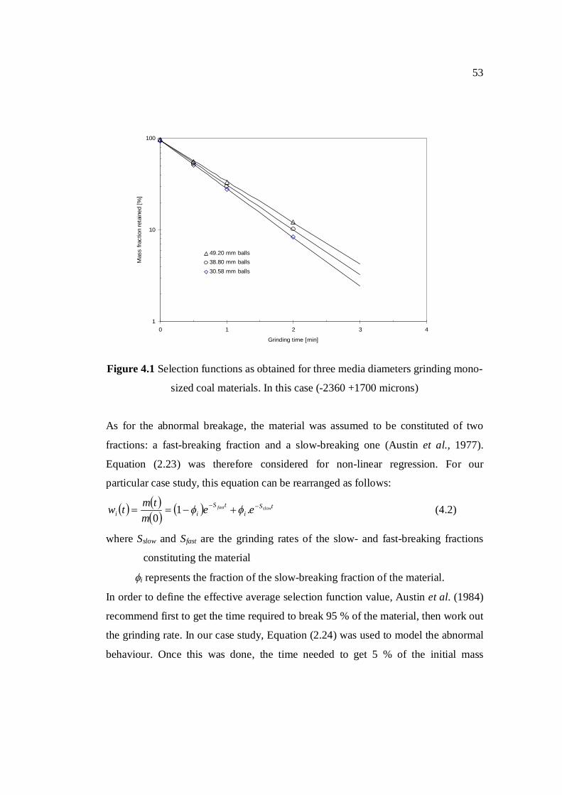
4.2.2 Determination of selection function parameters 54

4.3 Effect of ball size 55

4.3.1 Breakage rate as a function of ball size 55

4.3.2 Reduced selection function 56

4.4 Breakage distribution function 57

4.5 Significance of results (Interpretation) 60

4.6 Summary 61

Chapter 5 Effect of ball size distribution on milling kinetics 62

5.1 Introduction 62

5.2 Selection function of ball mixtures 63 5.2.1 Equilibrium ball size distribution 63

5.2.2 Original equipment manufacturer recommended ball size

distribution

64

5.3 Results and discussion 65 5.3.1 Ball size distribution effect 65

5.3.2 Validation of ball mixture model 67

5.3.3 Significance of findings 68

5.4 Summary 70

Chapter 6 Conclusion 71

6.1 Introduction 71

6.2 Summary of findings 71 6.2.1 Ball size effect 71

6.2.2 Ball size distribution effect 72

8

6.3 Overall conclusion 72

References 74

Appendices 81

A Results of particle size analysis 82 A.1 Batch grinding tests on single ball sizes 82

A.1.1 Particle size distributions obtained using 30.6 mm balls 82



A.2 Batch grinding tests on mixtures of balls 88

A.2.1 Particle size distributions obtained for the EQM-BSD 88

A.2.2 Particle size distributions obtained for the OEM-BSD 92

B Selection function results for different batch tests 96

C Reduced selection function after Snow 97 C.1 Maximum selection function values for different ball diameters 97

C.2 Reduced selection function values 97

D Manipulated data used in the determination of breakage function 98

E Prediction of the selection function of ball mixtures 100 E.1 Determination of milling parameters in each ball size interval 100

E.2 Predicted EQM- and OEM-BSD’s selection functions 100

E.3 Statistical analysis of the predictions 101

9

List of figures

Figure Page

2.1 Breakage mechanisms in a ball mill 22

2.2 First order reaction model applied to milling 24

2.3 Grinding rate versus particle size for a given ball diameter 25

2.4 Cumulative breakage function versus relative size 28

2.5 Predicted variation of Si values with ball diameter for dry grinding of

quartz

31

2.6 Breakage zones identified in a ball load profile 33

2.7 Breakage function of a 850×650 microns normalizable quartz under

various mill load conditions (D=195 mm, d=25.4 mm, c=0.7)

41

3.1 Snapshot of the laboratory mill 44

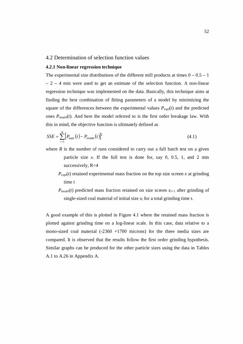
4.1 Selection functions as obtained for three media diameters grinding

mono-sized coal materials. In this case (-2360 +1700 microns)

54

4.2 Effect of ball diameter on the selection function 55

4.3 Reduced selection function graph 56

4.4 Reduced cumulative breakage function 58

5.1 EQM and OEM ball mass size distributions used 64

5.2 EQM and OEM ball number size distributions used 65

5.3 EQM-BSD graph as predicted with Equation (5.1) 66

5.4 Comparison of the predicted and measured selection on OEM-BSD 67

5.5 Modelled kinetics of the ball size distributions 68

10

List of tables

Table Page

3.1 Laboratory operating conditions 44

3.2 Ball mixtures used for experiment. 45

3.3 Experimental design 47

3.4 Mono-sized media charges used 47

4.1 Selection function parameters 54

4.2 Breakage function parameters for different ball size distributions 58

6.1 Tutuka coal breakage characteristics 71

A.1 Results of size analysis for + 16000 – 13200 microns coal using 30.6 mm balls 82











A.12 Results of size analysis for + 26500 – 22400 microns coal for EQM-BSD 88






11


A.19 Results of size analysis for + 300 –212 microns coal for EQM-BSD 91

A.20 Results of size analysis for + 26500 – 22400 microns coal for OEM-BSD 92







B.1 Selection function values for different batch grinding tests 96

C.1 Particle size corresponding to maximum selection function values for the single

sizes of ball

97

C.2 Reduced particle size and selection functions for the single sizes of balls 97

D.1 Breakage function obtained for the single ball sizes 98

D.2 Data used to assess size distributions normalization 99

E.1 Predicted selection function parameters in the different ball intervals used 100

E.2 Predicted selection functions for the two ball size distributions and the different

ball intervals used

100

E.3 Coefficient of determination for the EQM-BSD 101

E.4 Coefficient of determination for the OEM-BSD 101

12

List of symbols

a or a(d) Parameter characteristic of the material

A Material-dependent constants in Equations (2.16) and (2.17)

A' Material-dependent constants in Equations (2.16) and (2.17)

Ao Material dependent constant in Equation (2.12)

Ar Constant showing the material strength

B Material-dependent constants in Equations (2.16) and (2.17)

B' Material-dependent constants in Equations (2.16) and (2.17)

iib Parameter defined in Equations (2.23) and (2.24)

bi,j Mass fraction arriving in size interval i from breakage of size

interval j

jib , Mean breakage function of particles of size j breaking into size i

corresponding to a ball mixture

bi,j,k Fractional breakage into size i from breakage of size j by size k

balls

Bi,j Cumulative breakage function of particles of size xj into size xi

c Constant deduced from experimental data in Equation (2.15)

C' Proportionality constant in Equation (2.13)

C1 Constant as defined in Equation (2.19)

1C Constant as defined in Equation (2.20)

C2 Constant as defined in Equation (2.19)

2C Constant as defined in Equation (2.20)

d Ball diameter

dk Diameter of balls in the makeup

dmin Diameter of the ball leaving the mill after being worn down

dmax Maximum diameter of ball in the charge

13

do Material dependent constant in Equation (2.12)

fc Fraction of mill volume occupied by the bulk volume of powder

charged

k Wear law constant whose dimensions depend on the value of in

Equation (2.27)

k1 Constant which represents rate of change of radius in Bond wear

law

K Maximum breakage rate factor

m Constant as defined in Equation (2.19)

Mb Mass of a ball

mk Weight fraction of balls in class size k, relative mass frequency

function of balls of size dk I0m Relative number frequency of balls in the makeup

m(t) or mi(t) Mass fraction of particles of size i at time t ssM 3 Cumulative mass distribution of balls at steady-state

n Number of ball sizes

n0 Constant as defined in Equation (2.19)

dN Fraction by number of media with radii greater than d

p Number of ball classes in the makeup

Pc(x) Probability of crushing a particle of size x nipped by two

colliding balls

Pexpt(t) Retained mass fraction on top size screen x at grinding time t as

experimentally measured

Pi(t) Weight fraction of the material less than size xi at time t

Pmodel(t) Predicted mass fraction retained on size screen x after grinding of

single-sized material of initial size x for a total grinding time t

Pn(x) Probability of nipping a particle of size x by two approaching

balls

14

q(x) Function describing the probability of crushing nipped particles

Q(x) or Q(xi) Correction factor of the selection function equation in the

abnormal breakage region

rb Ball radius

r2 Coefficient of determination also called R-squared value

R Total number of runs required to carry out a full batch test on a

given particle size x

se Standard error of estimate

Si or Si(d) Rate of disappearance of material of size i or specific rate of

breakage of particles of size xi, also known as selection function

Si,k or Si(dk) Selection function of particle size xi due to balls of size dk

Sm Maximum value of the selection function for given ball and mill

diameters

S Weighted mean value of Si for the mixture of ball sizes in the mill

SSE Objective function defined as the Sum of Squared Errors

t Time defined for the grinding process or the wear mechanism

xi Size of particles in class i; for a size interval the upper size used

to represent the particle size

xm Particle size for which Si is maximum for given ball and mill

diameters

U Unit step function

VG Volume of the zone of possible nipping in the grinding zone

VM Mill volume

Vr Mean relative velocity of ball

wi(t) Mass fraction of unbroken material of size i in the mill at time t

Zef Frequency of collisions effective for crushing

α Parameter characteristic of the material

β Breakage parameter characteristic of the material used whose

values range from 2.5 to 5

15

G Material dependent constant in Equation (2.12)

N Constant independent of material and operational conditions

γ Breakage parameter characteristic of the material whose values

typically are found to be between 0.5 and 1.5

G Material dependent constant in Equation (2.12)

Wear rate factor defining the ball wear law

p Void fraction of the static bed in a tumbling ball mill

Exponent factor in Equation (2.11)

N Constant independent of material and operational conditions

Exponent factor in Equation (2.10)

Average ball-ball distance in the grinding zone. It has been shown

to vary with mill operating conditions

Λ Positive number representing an index of how rapidly the rate of

breakage falls as size increases in the abnormal region

µ or µ(d) Particle size at which the correction factor Q(x) is 0.5 for a ball

diameter d, it varies with mill conditions

i Fraction of slow-breaking material in Equations (2.23) and (4.2)

Φj Breakage parameter characteristic of the material used, it

represents the fraction of fines that are produced in a single

fracture event

Maximum life of the media in the mill due to wear

16

Chapter 1 Introduction

1.1 Background

For many decades milling has been the subject of intensive research. Describing and

understanding the process has been challenging because of the chaotic environment

of the tumbling mill itself. Mathematical models obtained so far are mainly based on

a mechanistic approach of the phenomenon. Despite the limitation of these models,

results produced have proven to be satisfactorily to a great extent.

As far as reliability and mechanical efficiency are concerned, tumbling ball mills are

the preferred choice for size reduction.

The problem with tumbling ball mills is that they are extremely wasteful in terms of

energy consumed (Wills, 1992). Therefore, the benefit of describing as accurately as

possible the grinding environment will not only help better understand the process

itself but also improve the use of available energy.

In order to do so, several factors influencing the process are to be considered.

Certainly, the starting point would be some investigation of the mill load behaviour

since it plays a paramount role in the overall grinding mechanism.

The major factors directly influencing the load behaviour are the constitution of the

charge, the speed of rotation of the mill, and the type of motion of individual pieces

of medium in the mill (Gupta and Yan, 2006). Mill speed and liner profile are

generally fixed operating parameters considering the fact that liners wear very

slowly. As a result, the type of motion of particles does not change on average. This

implies on an industrial point of view that flexibility will be most of the time limited

only to the constitution of the charge.

Concha et al. (1992) were able to get a 12% increase in capacity of an industrial mill

circuit by systematically optimizing the ball charge mixture. Hence, particular

attention should be paid to making sure that the charge is sensibly controlled. For

17

this reason, a clear description of the effect of mill load composition will allow one

to better model the grinding process and thereby provide a tool to find possible

increases in mill performance.

1.2 Statement of the problem

Coal is one of the most important commodities of South Africa. The mineral industry

and energy production sector are highly dependent on it. In the country, it is the

primary source used in the production of energy for mining industry and

miscellaneous needs. Basically, coal is mined, then pulverized and finally send to the

boiler for electricity production.

Coalfields on the planet are divided into two broad regions: the Gondwana and the

Laurasia. The Gondwana region refers to coals that are found mainly in the Southern

hemisphere. It includes Southern African coals, as well as those in India, Australia,

and South America. The Laurasian region on the contrary includes the carboniferous

coals found in the northern hemisphere.

In general, coals of the Gondwanaland have been found to be highly variable in rank

(maturity) and organic-matter composition compared to their counterparts in the

Laurasia. The major differences between the Carboniferous coals of the northern

hemisphere, and those found in the southern hemisphere reside in their respective

petrographic properties.

Falcon and Falcon (1987) have investigated the effects of this differentiation on the

combustion performance of coal. They showed that the petrographic characteristics

(i.e. organic composition and rank) of coals play a very important role in combustion

behaviour. The study also revealed dramatic differences between northern and

southern coals in terms of combustion characteristics. In this regard, the rank of coal

that defines the degree of transformation undergone by the seam through the

processes of time, temperature, or pressure in the in-depth rock mass could also

influence the mechanical properties of coal.

18

Later on, Falcon and Ham (1988) reported that except for the South Rand and

Orange Free State Coalfields, the European coals are in general much easier to grind

than those of Southern Africa.

The presence of syngenetic mineral matters (as opposed to secondary or epigenetic

minerals filling cracks or fissures) disseminated in the matrix is believed to increase

the strength of southern coals (Falcon and Falcon, 1987). This is due to the fact that

syngenetic mineral matters are formed at the same time as the enclosing rock and

therefore make the deposit to be more compact. Epigenetic minerals, on the other

hand, are formed after the enclosing rock has been formed.

Published results of laboratory tests on coal for comminution purposes have reported

findings that would be applicable specifically to the Laurasian coals (Austin et al.,

1984).

Because of the very limited information available on the South African coals, many

of the grinding parameters obtained on other coals have been used as default values.

However, coal properties vary markedly amongst seams, coalfields, and regions of

the world. Now, the question is: Is it sensible to consider South African coals to be

similar to Laurasian ones in terms of grinding performance?

1.3 Research objective

The well accepted Population Balance Model requires for its use a complete

breakage characterization of the material being described in terms of selection and

breakage functions. In order to achieve this, a series of laboratory tests need to be

carried out on a material sample under consideration.

In the present dissertation the applicability of the population balance model on a

South African coal is addressed. Some breakage parameters are reviewed to find

suitable values for South African coals. Specifically, the breakage kinetics of coal in

relation to the diameter of grinding media is studied. The aim is to fix definitely the

basis for breakage parameter estimation of South African coals in general. By the

same token, an attempt to clarify some issues pertaining to the effect of ball diameter

19

on milling rate. Then, the effect of ball mixture on the breakage rate parameters of

coal is assessed to provide valuable information for the simulation of industrial mills

used in Eskom Power Stations. Focus is allocated only on the dependence of the

selection function with respect to ball charge composition in the mill.

Discussion of the influence of the petrographic properties of coal on breakage will

not be touch upon as it is beyond the scope of this dissertation. Such a question

remains to be extended for more detailed consideration. Moreover, the

characterization of breakage properties of coal will be limited to the feed coal

generally used at Tutuka Power station.

1.4 Layout of the dissertation

The dissertation is organized into six chapters with the first chapter being the

introduction. The second chapter presents a summary of relevant theory of milling.

The state of current knowledge is reviewed with emphasis on the effect of ball size

and ball size distribution on milling rate. In addition, the dependency between the

competent ball diameter needed to optimally break a coal particle of given size is

discussed.

The third chapter provides a detailed description of the laboratory work and

equipment used to achieve the objective. Different procedures, the experiment

design, and laboratory work involved are presented.

The fourth chapter aims at characterizing a South African coal in terms of breakage

kinetics. After collection of data from the Wits pilot mill, the necessary information

on the grinding process is compiled. This information is crucial for scale-up and

simulation purposes in future works.

The fifth chapter presents the effect of ball size distribution on milling parameters for

simulation of industrial cases. It provides a better understanding of this effect and

attempt to validate available models for scale-up purposes in Eskom plants.

The last chapter gives a summary of the important findings, their relevance, and

some recommendations for future investigation.

20

Chapter 2 Literature Review

2.1 Introduction For many decades milling has been dealt with as a black box. In this technique, a

single operation is reduced to a box with an input and an output. Then, the mill

product size is estimated as a function of size and hardness of the mill feed, and

milling operating conditions (Napier-Munn et al., 1996).

A more realistic approach is the so-called Population Balance Model. In this

approach, the full description of the process reduces to two key components, namely

the Selection function and the Breakage function. Using these two functions simple

mass balances are constructed for each size fraction and following this the overall

operation is modelled.

A summary of the key elements describing the population balance model is

presented in this chapter, that is, selection and breakage functions. The

interdependence between these functions and mill conditions, specifically the size of

the grinding media and the ball size distribution of the charge, is also discussed.

2.2 Breakage mechanism in tumbling ball mills Several mechanisms contribute to the grinding action that takes place inside a mill.

These include impact or compression, chipping, and abrasion. These mechanisms

deform particles beyond their limits of elasticity and cause them to break (Wills,

1992).

The relative motion between media is responsible to a great extent for the grinding

action. Ball media are entrained in a tumbling motion which engenders some

interactions. During these interactions media collide or roll over each other.

Depending on the type and the magnitude of the interaction, particles break

following a certain pattern. King (2001) argued that in a ball mill particles break

21

primarily by impact or crushing and attrition. It seems however that impact breakage

is predominant at coarser particle sizes whilst attrition is the main reduction

mechanism at finer sizes. In between the two extremes, breakage is composed of

some combination of impact and abrasion. For the purpose of this dissertation

breakage is considered to be a result of impact, abrasion, and attrition only. Other

types of breakage mechanisms are not discussed here.

2.2.1 Impact breakage

Breakage by impact occurs when forces are normally applied to the particle surface.

It is also referred to as breakage by compression. King (2001) expounded this

mechanism of fracture and showed that it encompasses shatter and cleavage.

Fracture by cleavage occurs when the energy applied is just sufficient to load

comparatively few regions of the particle to the fracture point, and only a few

particles result. The progeny size is comparatively close to the original particle size.

This type of fracture occurs under conditions of slow compression where the fracture

immediately relieves the loading on the particle. Fracture by shatter on the other

hand occurs when the applied energy is well in excess of that required for fracture.

Under these conditions many areas in the particle are over-loaded and the result is a

comparatively large number of particles with a wide spectrum of sizes. This occurs

under conditions of rapid loading such as in a high velocity impact (Kelly and

Spottiswood, 1982).

2.2.2 Abrasion breakage

Abrasion is seen as a surface phenomenon which takes place when two particles

move parallel to their plane of contact. Small pieces of each particle are broken or

torn out of the surface, leaving the parent particles largely intact. Abrasion fracture

occurs when insufficient energy is applied to cause significant fracture of the

particle. Rather, localized stressing occurs and a small area is fractured to give a

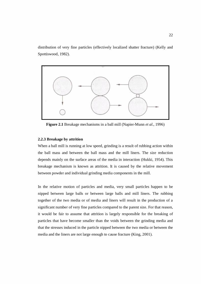
22

distribution of very fine particles (effectively localized shatter fracture) (Kelly and

Spottiswood, 1982).

Figure 2.1 Breakage mechanisms in a ball mill (Napier-Munn et al., 1996)

2.2.3 Breakage by attrition

When a ball mill is running at low speed, grinding is a result of rubbing action within

the ball mass and between the ball mass and the mill liners. The size reduction

depends mainly on the surface areas of the media in interaction (Hukki, 1954). This

breakage mechanism is known as attrition. It is caused by the relative movement

between powder and individual grinding media components in the mill.

In the relative motion of particles and media, very small particles happen to be

nipped between large balls or between large balls and mill liners. The rubbing

together of the two media or of media and liners will result in the production of a

significant number of very fine particles compared to the parent size. For that reason,

it would be fair to assume that attrition is largely responsible for the breaking of

particles that have become smaller than the voids between the grinding media and

that the stresses induced in the particle nipped between the two media or between the

media and the liners are not large enough to cause fracture (King, 2001).

23

2.3 Population balance model The objective of any operation of size reduction is to break large particles down to

the required size. In tumbling ball mills for instance, this operation is achieved

through repetitive actions of breakage. Modelling such a mechanism necessitates a

detailed understanding of the grinding process itself. Then, allowing for all the

operating variables and machine characteristics the feed and product size

distributions can be related.

Fragments from each particle that appear after first breakage consist of a wide range

of particle sizes. Some of the daughter fragments are still coarse and require further

breakage. The probability of further breakage depends on the machine design and

particle size.

The underlying physics suggests that the process is apparently a combination of two

actions taking place simultaneously inside the mill: a selection of the particle for

breakage, and a breakage resulting in a particular distribution of fragment sizes after

the particle is selected (Gupta and Yan, 2006). A size-mass balance inside the mill

that takes into account the two abovementioned reactions will make full description

of the grinding process possible. And eventually, mathematical relations between

feed size and product size, after comminution, can be developed.

2.3.1 Selection function

The disappearance of particles per unit time and unit mass due to breakage is

assumed to be proportional to the instantaneous mass fraction of particles of that size

fraction present inside the mill. This statement known as the first-order breakage

hypothesis is written as follows:

twSdt

tdwii

i (2.1)

where wi(t) represents the mass fraction of unbroken material of size i in the mill at

time t

24

Si is the rate of disappearance of material of size i, also known as selection

function.

Because the population balance model is based upon the first order grinding law it is

sometimes referred to as the “first order rate model” (Napier-Munn et al., 1996).

It is not yet established in theory why particles follow this law. Despite its simplicity

the law has proven to apply to numerous materials so far especially for fine sizes.

Research is currently being conducted in order to get much insight in the foundation

of this assumption. But until that is achieved, the model is reasonably good for many

materials over a wide range of operation (Austin et al., 1984; Napier-Munn et al.,

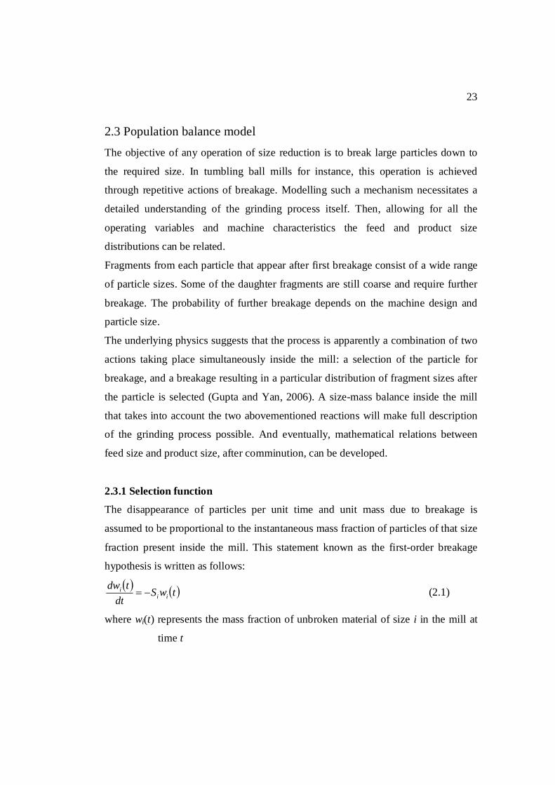
1996).

Figure 2.2 First order reaction model applied to milling after Austin et al. (1984)

(a) Normal breakage; (b) Abnormal breakage

Figure 2.2(a) shows the first-order breakage law for a given material. However,

substantial deviations from the first-order law are noted for coarse materials (Austin

et al., 1973). In this case breakage is said to occur in the abnormal region and is

illustrated in Figure 2.2(b). This behaviour is addressed later in this dissertation.

25

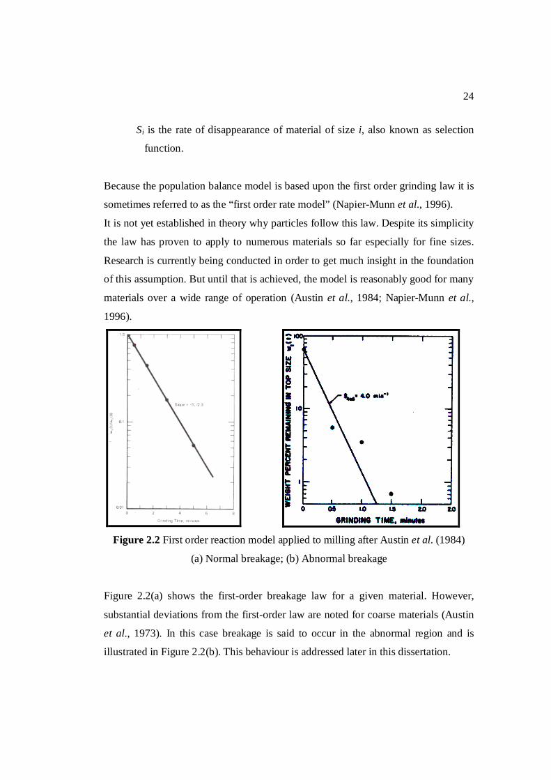
Perhaps the most important point is how the rate of breakage changes with respect to

particle size. According to Griffith theory of breakage (Austin et al., 1984), for the

same size of balls in a mill, very fine particles are hard to break. This suggests that as

the particle size increases the breakage rate should continuously increase. The

general observed trendline (Figure 2.3) agrees consistently with this statement. But

then comes a turning point after which particles become too large to be nipped by

balls. The rate of breakage steadily drops and tends to zero.

Figure 2.3 Grinding rate versus particle size for a given ball diameter (Austin et al., 1984)

Now, based on the results of several laboratory tests, Austin et al. (1984) were able

to show that the rate of disappearance of particles as a function of size is given by

i

iiiix

xaxQxaS

1

1... (2.2)

where xi is the particle size in class i in mm

26

α and a are parameters strongly dependent on the material used

µ defines the particle size at which Q(xi)=0.5, it varies with mill conditions

is an index allowing for the decrease in the value of the selection function

with increasing particle size

For finer materials, it is readily seen that Q(x) reduces to approximately 1, and

therefore Equation (2.2) becomes ii xaS . . The reduced equation geometrically

represents on log-log scale a straight line of which characteristics are the slope α (see

dotted line in Figure 2.3) and the breakage rate a at a standard particle size here

taken as 1 mm.

The parameter α is a positive number normally in the range 0.5 to 1.5. It is

characteristic of the material and does not vary with rotational speed, ball load, ball

size or mill hold-up over the normal recommended test ranges (Austin and Brame,

1983) for dry milling, but the value of a will vary with mill conditions.

In the correction factor Q(x), is a positive number which is an index of how

rapidly the rates of breakage fall as size increases: The higher the value of , the

more rapidly the values decrease. The parameter is found to be primarily a

characteristic of the material.

2.3.2 Breakage function

The breakage function, better called the primary breakage distribution function, can

be defined as the average size distribution resulting from the fracture of a single

particle (Kelly and Spottiswood, 1990).

After a single step of breakage of a particle, the distribution of sizes produced is

described in terms of breakage or appearance function. Thus the relative distribution

of each size fraction after breakage is perceived as a full description of the product.

That is why the primary breakage distribution function of a particle of size j to size i

is defined as follows:

27

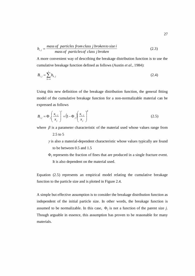
brokenj class of particles of massi sizeto brokenj class from particles of massb ji , (2.3)

A more convenient way of describing the breakage distribution function is to use the

cumulative breakage function defined as follows (Austin et al., 1984):

i

nkjkji bB ,, (2.4)

Using this new definition of the breakage distribution function, the general fitting

model of the cumulative breakage function for a non-normalizable material can be

expressed as follows

j

ij

j

ijji x

xxxB 11

, 1 (2.5)

where is a parameter characteristic of the material used whose values range from

2.5 to 5

is also a material-dependent characteristic whose values typically are found

to be between 0.5 and 1.5

j represents the fraction of fines that are produced in a single fracture event.

It is also dependent on the material used.

Equation (2.5) represents an empirical model relating the cumulative breakage

function to the particle size and is plotted in Figure 2.4.

A simple but effective assumption is to consider the breakage distribution function as

independent of the initial particle size. In other words, the breakage function is

assumed to be normalizable. In this case, j is not a function of the parent size j.

Though arguable in essence, this assumption has proven to be reasonable for many

materials.

28

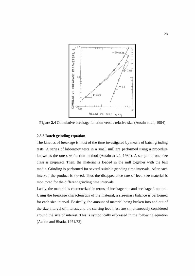
Figure 2.4 Cumulative breakage function versus relative size (Austin et al., 1984)

2.3.3 Batch grinding equation

The kinetics of breakage is most of the time investigated by means of batch grinding

tests. A series of laboratory tests in a small mill are performed using a procedure

known as the one-size-fraction method (Austin et al., 1984). A sample in one size

class is prepared. Then, the material is loaded in the mill together with the ball

media. Grinding is performed for several suitable grinding time intervals. After each

interval, the product is sieved. Thus the disappearance rate of feed size material is

monitored for the different grinding time intervals.

Lastly, the material is characterized in terms of breakage rate and breakage function.

Using the breakage characteristics of the material, a size-mass balance is performed

for each size interval. Basically, the amount of material being broken into and out of

the size interval of interest, and the starting feed mass are simultaneously considered

around the size of interest. This is symbolically expressed in the following equation

(Austin and Bhatia, 1971/72):

29

1

1,

i

jjjjiii

i twSbtwSdt

tdw (2.6)

where Si is the selection function of the material considered of size i

wi(t) is the mass fraction of size i present in the mill at time t

bi,j is the mass fraction arriving in size interval i from breakage of size interval j.

From then on, the particle size distribution of the material being milled can be

predicted at any time along the process using Equation (2.6).

2.4 Effect of ball size Experience shows that small balls are effective for grinding fine particles in the load,

whereas large balls are required to deal with large particles. In addition, harder ores

and coarser feeds require high impact energy and large media. And on the other

hand, very fine grind sizes require substantial media surface area and small media

(Napier-Munn et al., 1996).

Finding the right size of balls for a specific feed material to ensure grinding

efficiency has always been a challenge. An empirical rule which has been used for

many years shows that there is a relationship between the size x of the particle to be

ground and the ball diameter d. It is given by xm=K.d2 where K is the maximum

breakage rate factor. On the one hand, Austin et al. (1976) reported that K is a

constant of which value range from 10-3 to 0.7×10-3 for soft to hard materials; and on

the other hand, Napier-Munn et al. (1996) found K to be in the order of 0.44×10-3.

In this section the different equations used to address this question are revised.

Empirical approaches are here based on experiments whereas theoretical ones are

based on analytical descriptions of the process.

2.4.1 Empirical approaches

The selection function can be expressed by the following general equation

iii xQxdaS .. (2.7)

30

where xi is the size of the particle

d is the diameter of the media used for the test

Q(xi) is a correction factor

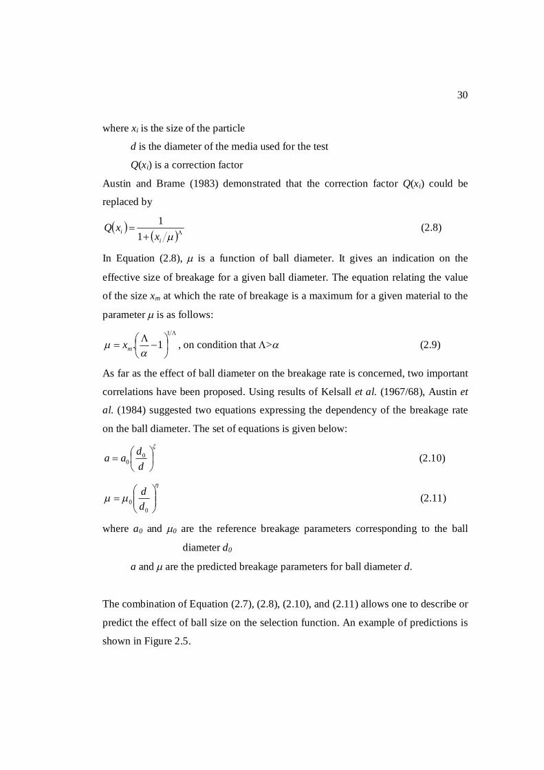
Austin and Brame (1983) demonstrated that the correction factor Q(xi) could be

replaced by

i

i xxQ

11 (2.8)

In Equation (2.8), is a function of ball diameter. It gives an indication on the

effective size of breakage for a given ball diameter. The equation relating the value

of the size xm at which the rate of breakage is a maximum for a given material to the

parameter is as follows:

1

1.

mx , on condition that > (2.9)

As far as the effect of ball diameter on the breakage rate is concerned, two important

correlations have been proposed. Using results of Kelsall et al. (1967/68), Austin et

al. (1984) suggested two equations expressing the dependency of the breakage rate

on the ball diameter. The set of equations is given below:

ddaa 0

0 (2.10)

00 d

d (2.11)

where a0 and 0 are the reference breakage parameters corresponding to the ball

diameter d0

a and are the predicted breakage parameters for ball diameter d.

The combination of Equation (2.7), (2.8), (2.10), and (2.11) allows one to describe or

predict the effect of ball size on the selection function. An example of predictions is

shown in Figure 2.5.

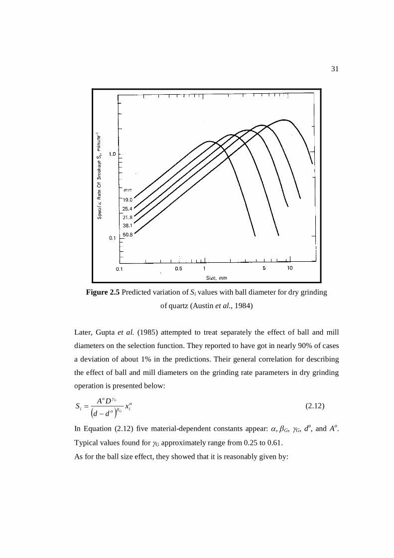
31

Figure 2.5 Predicted variation of Si values with ball diameter for dry grinding

of quartz (Austin et al., 1984)

Later, Gupta et al. (1985) attempted to treat separately the effect of ball and mill

diameters on the selection function. They reported to have got in nearly 90% of cases

a deviation of about 1% in the predictions. Their general correlation for describing

the effect of ball and mill diameters on the grinding rate parameters in dry grinding

operation is presented below:

io

o

i xddDAS

G

G

(2.12)

In Equation (2.12) five material-dependent constants appear: ,G, G, do, and Ao.

Typical values found for G approximately range from 0.25 to 0.61.

As for the ball size effect, they showed that it is reasonably given by:

32

dCda

1 (2.13)

where is a parameter that has been shown to be independent on mill diameter for

the same combination of media sizes

C' is a proportionality constant.

Another equation that is worth mentioning is the equation of Snow. Austin et al.

(1976) reported the following expression:

m

i

m

i

m

i

xx

xx

SS exp

(2.14)

where xm is the feed size at which Si is the maximum value Sm.

Some researchers claim that this type of equation is not suitable for describing the

selection function (Austin et al., 1976; Kotake et al., 2002). It seems to them that

Equation (2.14) cannot sufficiently explained the dependency of the dimensionless

grinding rate constant Si/Sm on the feed size xi. On top of that, a careful look at it

reveals the equation to be invalid. Simply put, for xi equal to xm, Si should be equal to

Sm, which is not the case. For this reason, Kotake et al. (2004) revised Snow’s

equation and proposed the following:

m

mi

m

i

m

i

xxxc

xx

SS

exp.

(2.15)

where and c are constants deduced from experimental data.

Perhaps, the most important point is that Equations (2.14) and (2.15) bring up the

notion of normalized or reduced Si and xi values. The dimensionless breakage rate

and feed size are defined as Si/Sm and xi/xm respectively. It allows one to reduce all

the selection curves corresponding to different ball diameters into one single curve

with normalized feed size and grinding rate respectively on the x- and y-axes. As for

the effect of ball size, the following relationships are used for Snow’s equation

(Kotake et al., 2004):

33

Bm dAx . (2.16)

Bm dAS . (2.17)

where A, B, A', and B' are material-dependent constants.

2.4.2 Probabilistic approaches

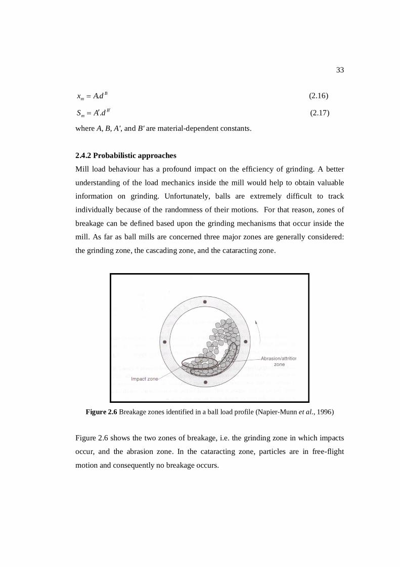
Mill load behaviour has a profound impact on the efficiency of grinding. A better

understanding of the load mechanics inside the mill would help to obtain valuable

information on grinding. Unfortunately, balls are extremely difficult to track

individually because of the randomness of their motions. For that reason, zones of

breakage can be defined based upon the grinding mechanisms that occur inside the

mill. As far as ball mills are concerned three major zones are generally considered:

the grinding zone, the cascading zone, and the cataracting zone.

Figure 2.6 Breakage zones identified in a ball load profile (Napier-Munn et al., 1996)

Figure 2.6 shows the two zones of breakage, i.e. the grinding zone in which impacts

occur, and the abrasion zone. In the cataracting zone, particles are in free-flight

motion and consequently no breakage occurs.

34

The theory of probability helps to get much insight on the general behaviour of the

load. Most of the breakage takes place in the grinding zone in which balls in free-fall

motion impact the material. The cascading zone is more prone to abrasion. In the

cataracting zone, particles and media are in flight motion; as a result, nothing much

happens in terms of breakage.

Nomura et al. (1991) tried to model breakage using the notion of breakage zones.

Although various mechanisms of size reduction occur in the mill, impact breakage

has been considered to be dominant in milling by balls. Basically, for breakage by

impact to take place, a particle is to be nipped, or caught between two colliding balls,

then crushed with sufficient collision energy. To describe this, two probabilities were

introduced: the probability of nipping a particle in a single collision, and the

probability of crushing a nipped particle by collision.

Nomura et al. (1991) then defined the specific rate of breakage or selection function

as the fracture probability of a particle. The probabilistic definition of the selection

function is given below:

Mc

cnGef

VfxPxPVZ

xS (2.18)

where Zef is the frequency of collisions effective for crushing

VG is the volume of the zone of possible nipping in the grinding zone

Pn(x) is the probability of nipping a particle of size x by two approaching balls

Pc(x) is the probability of crushing a particle of size x nipped by two colliding

balls

fc is the fraction of mill volume occupied by the bulk volume of powder

charged

VM is the mill volume.

Using appropriate simplistic assumptions, Kotake et al. (2004) derived the following

theoretical equation:

021 exp n

ii

mi d

xCxdCS (2.19)

35

where C1, C2, m and n0 are constants.

Letting m=0.25 and n0=1 Equation (2.19) reduces to:

dxCxdCS i

ii 225.0

1 exp (2.20)

derived by Tanaka and in which 1C and 2C are constants.

The key point in Tanaka’s equation is that it can be utilized to investigate the change

of the grinding rate constant as a function of ball diameter and feed size.

As for Nomura et al. (1991), the theoretical selection function was derived as follows

31

21351

11

b

b

Mc

ef

dxxxqx

VfCZ

xS

(2.21)

where Zef is the frequency of collisions effective for crushing

is the average ball-ball distance in the grinding zone. It has been shown to

vary with mill operating conditions

C1 is given by 21 2

16 rbpr

NN VMA

C

with Ar is a constant showing the

material strength, and N and N are constants independent of material and

operational conditions. Mb is the mass of a ball whereas Vr is the mean

relative velocity of ball. And p represents the void fraction of a static bed.

q(x) is a function of the probability of crushing of a nipped particle.

Substituting the following a=ZefC1/(fc.VM.) and α=(5b/3)+1 into Equation (2.21)

allows to get back to Equation (2.7), but this time with the corresponding correction

factor given by

31

2

11

bdxxxqxQ

where α, defined as a distribution parameter, now proven theoretically to be material

characteristic as usually assumed in empirical models.

However, for practical milling, q(x) and the denominator of Q(x) have been found to

be close to unity, leading to the following expression

36

21 xxQ (2.22)

Finally, the effects of the ball diameter and density on a are experimentally (Nomura

et al., 1991) found to be related as follows: da b .

2.5 Abnormal breakage Abnormal breakage in laboratory mills may be defined as departure from first-order

kinetics, and occurs particularly for the larger particle sizes in the mill feed (Austin

et al., 1973). Later on, Austin et al. (1977) studied the abnormal breakage and

proposed several models that may explain it. First, they assumed the material to

consist of an initial material A that breaks to produce another material B. The two

materials are different only on a breakage point of view. Then, during grinding,

component A is breaking to component B. In doing so, they found the following

model:

tS

itS

iiBA ee

mtmtw .10

(2.23)

where BA

Aiii SS

Sb

SA is the selection of component A of the material

SB is the selection function of component B of the material.

In overall, the system behaves as if the A material consists of a fraction 1-i of soft

material and a fraction i of harder material.

In general the effective mean value of the selection function is given by

Bi

ii

Ai

i

Sb

S

S

11 (2.24)

Because not all the non-first-order grinding batch grinding can be fitted with

Equation (2.23), a more elaborated has been proposed. Second, they assumed the

37

feed A breaking to an intermediate material B which in turn breaks to a final material

C. The corresponding model is as follows:

tS

CA

AtSAC

CA

AA

i

ii

CA eSS

SetSSSS

StSm

tmtw

22

.110

(2.25)

Here the effective mean value of the milling rate is approximately given by

CiBiAi

i

SSS

S 1111

(2.26)

In conclusion, for larger sizes, it is found that the disappearance of material from a

given top size interval is often not first order, but can be modelled as consisting of a

faster initial rate and a slower following rate. We refer to the first-order breakage of

smaller sizes as normal breakage and to the non-first-order breakage of larger sizes

as the abnormal breakage region. When a particle size exhibits an abnormal

behaviour, Austin et al. (1984) suggests the mean effective specific rate to be defined

by the time required to break 95% of the material. Alternatively Equation (2.24) can

be used.

2.6 Effect of ball mixture 2.6.1 Ball size distribution in tumbling ball mills

During the grinding operation, the object is to hold an equilibrium charge where the

rate of addition of the number and mass of balls equals the rate at which the number

of balls are eroded and expelled from the mill plus the rate of loss in mass of balls

due to abrasion and wear. That is, the grinding conditions remain constant. The

initial charge should be as identical as possible to the equilibrium charge.

The ball charge in a mill is never constituted of uniform sizes of balls; it is rather a

mixture of balls of different sizes ranging from small up to bigger balls that are

newly added.

One of the most difficult questions to address and indeed the most important to

answer in the optimal design of ball milling circuits is the choice of the mixture of

38

ball sizes to be used in the mills. Plants have generally developed in-house solutions

to this problem.

The equilibrium ball size distribution is a function of the makeup policy and the wear

mechanism. Menacho and Concha (1986) have addressed this issue. They considered

the general model of ball wear in a mill proposed by Austin and Klimpel (1986):

2. bb rk

dttdM (2.27)

where Mb(t) is the ball mass after time t

rb is the ball radius

k is a constant whose dimensions depend on the value of

is a constant defining the ball wear law.

In the differential equation (2.27), it is assumed that the mass wear rate of a piece of

spherical media (mass per unit time) is a power function of its radius r. Thus if =0,

the wear rate is proportional to the surface area of the ball. It is called the Bond wear

law or the surface law. On the contrary, if =1, the ball wear follows the Davis wear

law or the mass wear law.

Experimental data have reported a -value of 2 can also be obtained especially for

wet milling (Austin and Klimpel, 1985).

Using a phenomenological approach, Menacho and Concha (1986) have derived the

solution of Equation (2.27). Their solution represents in fact a general model for the

dynamic ball size distribution in a ball mill.

With appropriate assumptions, the steady-state ball size distribution can be deduced.

And if the wear law is given ( is given), the general steady-state ball size

distribution model is expressed as follows:

p

kkk

p

kkkk

ss

dddm

ddUdddmdddM

1

44I0

1

44I0

40

4

3 (2.28)

where ssM 3 is the cumulative mass distribution of balls at steady-state

39

dk is the diameter of balls in the makeup

d is the diameter of balls in the charge

is the wear rate factor I0m is the relative number frequency of balls in the makeup

p is the number of ball classes in the makeup

U is the unit step function defined as follows

0for 10for 0

dd

dU

For respectively one and two ball sizes in the makeup, Equation (2.28) can be

reduced to the equilibrium ball size distribution proposed by Austin and Klimpel

(1985):

4min

4max

4min

4

dddddM , for one ball size (2.28)

124min

421

411

4min

421

41

2min4min1

411

4min

4

for 11

for 1

dddddKdKddKdK

ddddKdK

dd

dM , for two ball sizes (2.30)

where

13

2

1

1

21 1

dd

mmK and thus lies between 0 and 1.

For a single ball size d in the makeup Equation (2.29) applies, whereas Equation

(2.30) is used for a makeup of balls consisting of two ball sizes d1 (d1=dmax) and d2

for which mass fractions are m1 and m2 respectively.

If the ball wear follows the Bond law, that is =0, it is possible to show that the

fraction number of media in the mill at steady-state is related to the diameter of the

balls as follows (Yildirim and Austin, 1998):

dNd

kd

d .2

1max

1

max

(2.31)

where dN is the fraction by number of media with radii greater than d

40

1maxmin 2kdd is the diameter of the ball leaving the mill after being

worn down

k1 is a constant which represents rate of change of radius in Bond wear law

is the maximum life of the media in the mill due to wear.

Equation (2.31) shows that the equilibrium charge consists of equal number of balls

in each ball class providing the class widths are the same. In other words, according

to Bond law, the equilibrium ball charge distribution is in statistical terms a constant

number distribution function.

2.6.2 Milling performance of a ball size distribution

The overall effect of a mixture in the mill may be taken as the linear weighted sum

(Austin et al., 1984),

m

kkik

m

kkiki SmdSmS

1,

1

(2.32)

where mk is the relative mass frequency function of balls of size dk.

Si(dk) is the selection function of particle size xi due to balls of size dk

Let bi,j,k be the fractional breakage into size i from breakage of size j by size k balls.

The mean breakage function is given by the ratio between the total specific rate of

breakage into size i and the total specific rate of breakage from size j, that is,

m

kkkj

m

kkkikjiji mSmSbb

1,

1,,,, (2.33)

If bi,j,k is not a function of k, Equation (2.33) reduces to jiji bb ,, .

We will assume this to be true, that is, one set of bi,j values only will be used. We

will further assume, on the basis of rather limited experimental information, that bi,j

values do not change with mill conditions or mill diameter in the region of usual

operating conditions. Figure 2.7 gives an illustration of a material of quartz that has

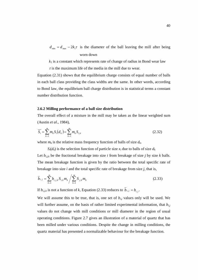
been milled under various conditions. Despite the change in milling conditions, the

quartz material has presented a normalizable behaviour for the breakage function.

41

Figure 2.7 Breakage function of a 850×650 microns normalizable quartz under

various mill load conditions (D=195 mm, d=25.4 mm, c=0.7) after Austin et al.

(1984)

2.7 Summary The review of the literature has revealed several key points that are listed below.

The widely accepted empirical form for the selection function model is given by:

)(.. xQxaS ii

where a is the grinding rate constant and α is the distribution parameter of the

material.

Q(x) is a correction function varying from 1 to 0 with increasing x but is rather

insensitive for relatively small x. The most important expressions factors that have

been reported so far for the correction factor Q(x) are the following:

1° xkxQ .exp (Austin et al., 1976; Kotake et al., 2004; Snow’s equation;

Tanaka’s equation)

42

2°

lnln xGxQ where

x

u duexG .21 22

is the Gaussian or normal

distribution function (Austin et al., 1976)

3°

x

xQ

1

1 (Austin et al., 1984)

The breakage function is generally regarded as normalizable for most of the

materials found.

The effect of ball size gives rise to several questions pertaining to and . Various

values of have been reported in the range 1 to 2, whilst has been about 1 (Kelsall

et al., 1967; Austin et al., 1976; Austin et al., 1984; Yildirim et al., 1999; Kotake et

al., 2004; Austin et al., 2006). Only a detail investigation on a South African coal

will allow to establish with confidence the values to use for our particular cases.

Considering the availability of the documentation at hand, the effect of ball size

distribution is accepted to be the weighed sum of the individual contribution of balls

to grinding.

In their conclusion, Concha et al. (1992) quoted the following: “Further progress will

require refinement of the mill simulator model, in particular more detailed

investigations of the effect of ball diameter on breakage rates, primary fragment

distributions and mill performance.” As a consequence of this statement, it is

believed that an investigation of the effect of ball size and ball size distribution on a

South African coal is worth the effort.

43

Chapter 3 Experimental equipment and programme

The Mineral Processing Research Group of the Centre of Material and Process

Synthesis (COMPS) initiated in October 2007 an industrial survey. The main

objective was to collect enough feed coal for this project from Tutuka Power Station

in South Africa. Media and mill feed coal had to be sampled for laboratory purposes.

A total coal mass sample of 250 kg was collected from a selected mill feed. And 150

kg of grinding media was carefully prepared from a regraded mill load. Three ball

sizes were considered: 30.6 mm, 38.8 mm, and 49.2 mm; and in each case, 50 kg of

media was constituted.

Using the Wits pilot mill, a series of batch tests had to be carried out under different

mill conditions. To fully characterize the breakage properties of this coal, three ball

sizes and two ball mixtures were used.

In this chapter, the experimental equipment and programme in the laboratory are

presented: how batch tests were done, particle size analysis, feed preparation, and

ball size preparation.

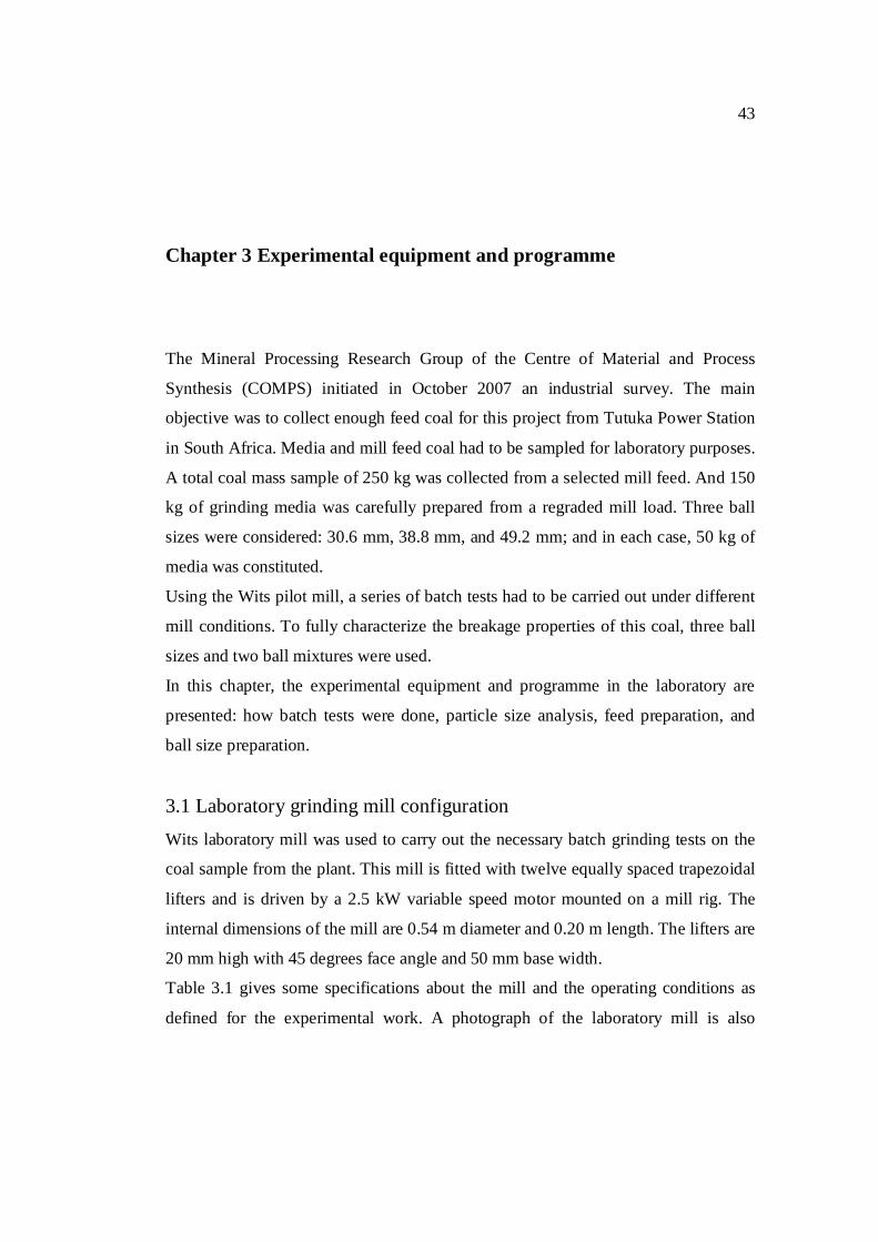
3.1 Laboratory grinding mill configuration Wits laboratory mill was used to carry out the necessary batch grinding tests on the

coal sample from the plant. This mill is fitted with twelve equally spaced trapezoidal

lifters and is driven by a 2.5 kW variable speed motor mounted on a mill rig. The

internal dimensions of the mill are 0.54 m diameter and 0.20 m length. The lifters are

20 mm high with 45 degrees face angle and 50 mm base width.

Table 3.1 gives some specifications about the mill and the operating conditions as

defined for the experimental work. A photograph of the laboratory mill is also

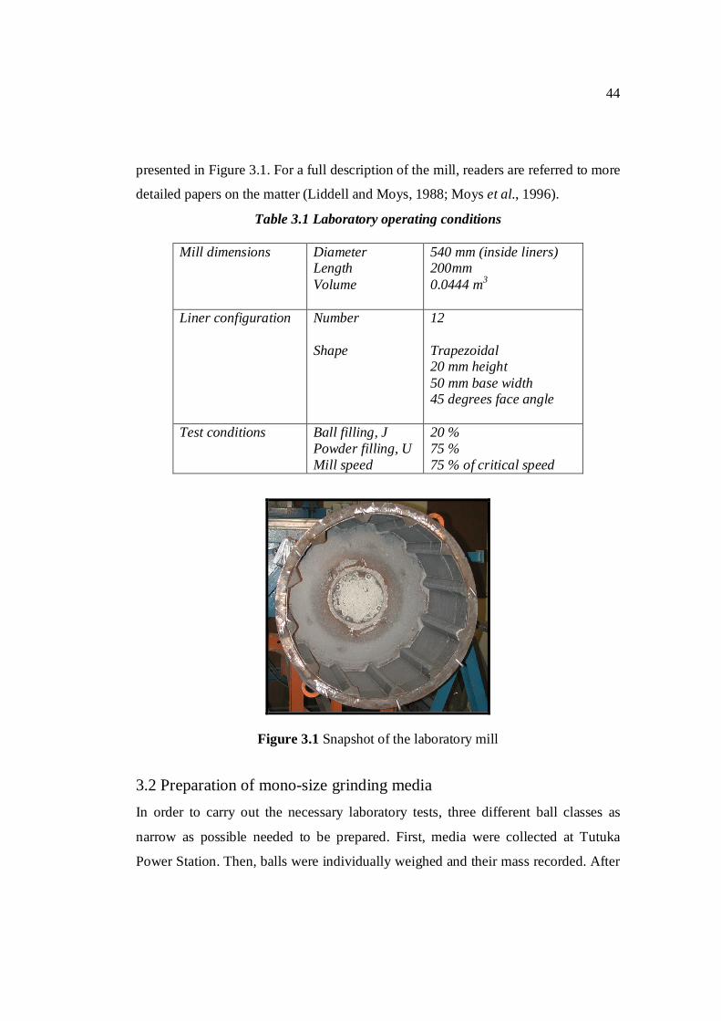
44

presented in Figure 3.1. For a full description of the mill, readers are referred to more

detailed papers on the matter (Liddell and Moys, 1988; Moys et al., 1996).

Table 3.1 Laboratory operating conditions

Mill dimensions Diameter Length Volume

540 mm (inside liners) 200mm 0.0444 m3

Liner configuration Number Shape

12 Trapezoidal 20 mm height 50 mm base width 45 degrees face angle

Test conditions Ball filling, J Powder filling, U Mill speed

20 % 75 % 75 % of critical speed

Figure 3.1 Snapshot of the laboratory mill

3.2 Preparation of mono-size grinding media In order to carry out the necessary laboratory tests, three different ball classes as

narrow as possible needed to be prepared. First, media were collected at Tutuka

Power Station. Then, balls were individually weighed and their mass recorded. After

45

data analysis, balls within predefined mass intervals were selected to constitute the

population of interest. With the ball density (7.62 g/cm3) and the mass ranges

defined, ball sizes could finally be calculated. Specifically, three sizes were retained:

30.6 mm, 38.8 mm, and 49.2 mm.

As far as the ball mixtures are concerned, two mixes were considered:

1 The first mixture was constituted of the same number of balls the six ball size

intervals considered. And for the purpose of comparison, this charge has been

called “Equilibrium Ball Size Distribution” EQM-BSD.

2 The second mixture, on the other hand, is constituted of the same mass of balls

in the six ball classes. It is here referred to as “Original Equipment Manufacturer

recommended Ball Size Distribution” OEM-BSD.

Equal numbers of balls in each size class results when the ball wear rate is constant

and a fixed top size of ball is fed to the mill. OEM-BSD on the contrary is

recommended by the OEM at Tutuka Power Station. It implies more balls of small

sizes, and consequently, an increase in the total surface area and an increase in the

rate of milling of fine particles.

Table 3.2 presents the two ball size distributions as considered for the tests. In each

case the mass of the load was calculated to be 41.2 kg for an average bed porosity of

0.4 (Austin et al., 1984).

Table 3.2 Ball mixtures used for experiment.

EQM-BSD OEM-BSD Ball classes

(mm) Mass fraction

(%) Ball number Mass

fraction (%) Ball number

50.0 – 44.0 40.0 40 16.6 17 44.0 – 37.5 25.8 40 16.7 27 37.5 – 31.5 15.8 38 16.6 37 31.5 – 26.5 9.3 38 16.7 70 26.5 – 22.4 5.6 40 16.7 126 22.4 – 19.0 3.4 40 16.7 224

46

3.3 Feed material preparation

3.3.1 Coal sample collection at Tutuka power station

A large coal sample was obtained from a mill feed at Tutuka Power Station for

laboratory tests. From the inlet of the mill, a sampling pipe was inserted into the feed

stream to collect coal samples. Twelve plastic bags were filled with approximately

20 – 25 kg of coal each. Globally, 250 kg of coal was collected.

Internal references reported the average coal particle density as established in routine

inspection at Tutuka Power Station to be 1.57 g/cm3. The humidity of the coal was

found after preliminary laboratory tests to be approximately 5.23 %.

3.3.2 Feed preparation for laboratory tests

With the test conditions defined in Table 3.1 the necessary mass of material

(powder) per test to be used was calculated to be 2.507 kg for a specific density of

1.57 g/cm3. Knowing this, a total of 26 mono-sized feed materials was prepared for

the intended series of grinding tests (Table 3.3).

The coal collected at the plant was first to be roughly sorted by particle size classes.

To do this, batches of approximately 2 kg of coal were one after another screened for

about 5 min. Fractions of coal retained on the screens of interest as depicted in Table

3.3 were accumulated in labelled plastic bags. After that, a further screening of 20

min on the sorted mono-sized coal in each plastic bag was done to get a bulk mono-

sized mass more carefully prepared. Finally, the different masses obtained which

were ready for batch testing were split using a Jones riffler to constitute 2.507 kg

representative feed coal samples. After this last step in the preparation, feed samples

were ready for batch test.

To sum up: on the one hand, eight single sized feed coal samples were prepared for

the EQM-BSD tests. And on the other hand, seven samples were considered for the

OEM-BSD. As for the single ball sizes 4, 4, and 3 feed sizes were constituted

respectively for tests using 49.2, 38.8, and 30.6 mm balls. Table 3.3 gives a summary

of the sizes that were milled in each case.

47

Table 3.3 Experimental design

Feed size (microns) Ball charge considered Upper Lower EQM-BSD OEM-BSD 30.6 mm 38.8 mm 49.2 mm 26 500 22 400 × × × 22 400 19 000 × 19 000 16 000 × × 16 000 13 200 × × 13 200 9 500 × × 9 500 6 700 × × 6 700 4 750 × × × 4 750 3 350 3 350 2 360 × × 2 360 1 700 × × × 1 700 1 180 × × 1 180 850

850 600 × 600 425 × 425 300 × 300 212 ×

3.4 Experimental procedures 3.4.1 Experiment design

The programme presented in Table 3.3 was designed and followed to achieve the

objective of the present study.

Tests on single ball sizes were used to determine the breakage characteristics of coal.

Table 3.4 presents the single sizes considered, their respective number for a total

mass of 41.205 kg in the mill load.

Table 3.4 Mono-sized media charges used

Ball size [mm] 30.6 38.8 49.2

Ball number 358 181 89

Total mass [kg] 41.205 41.205 41.205

48

To illustrate how Table 3.3 is to be used, one would infer that particles in the size

interval 9500 – 6700 microns was batch milled using 38.8 mm ball media. Another

example would be the size interval 300 – 212 microns and the EQM-BSD.

Mono-sized media charges presented in Table 3.4 will be used for characterizing the

breakage properties of the coal under study. Tests on the EQM-BSD are for

investigating the effect of ball size distribution on milling rate whereas those on the

OEM-BSD serve for validation.

3.4.2 Batch grinding tests

Broadly speaking, batch grinding tests are performed using the procedure known as

the one-size-fraction method (Austin et al., 1984).

In our experimental work, three grinding times were considered: 0 – 0.5; 0.5 – 1; 1 –

2 min. For every test, a blank sieving test was done on the prepared feed material.

After that, the coal sample was placed in the mill with the media of appropriate size.

The feed size and media size were mixed in accordance to the programme in Table

3.3. Next, the feed material was ground for 30 seconds; then, analyzed. The mill was

emptied after this time period through a grate to retain the grinding balls. A full

particle size distribution was done on the collected product from the top screen down

to the 75 microns screen.

First, the product was screened down to 1700 microns. Then, the undersize material

(i.e. -1700 microns) was split to constitute a 100 g representative sample. Second, the

100 g sample was wet washed on a 75 microns screen to remove the dust. Then, a

drying in the oven at 50°C followed. Finally the dried coal was screened to complete

the size analysis. For materials of size below 1700 microns, a 100 g sample was

directed prepared for wet screening, then dry screening after the washed sample was

dried in the oven.

After all this, the material was then recombined for batch grinding for an extra 30

seconds, followed by size analysis. The process was finally repeated for 60 more

seconds. As for materials of size less than 1700 microns, coal samples were milled

49

for a total time of 4 min, i.e. a fourth time period 2 – 4 min was added for the full

test.

3.4.3 Particle size analysis

Dry sieving was always performed for about 20 minutes. The complete size analysis

was made using a stack of sieves, starting with the top size of the feed size interval

all the way done to 75 microns.

For materials coarser than 1700 microns, size analysis was performed in two steps.

First, a dry screening of the material was done for 20 minutes down to 1700 microns.

Then, the material in the pan (-1700 microns) was split to obtain a 100 g mass

sample. The small sample was wet washed on a 75 microns screen to remove the

fines (-75 microns). Then, the washed sample was dried in the oven at 50C. The

dried sample was weighed, and then screened for 20 minutes using nested screens

from 1700 down to 75 microns.

For materials smaller than 1700 microns, size analysis was done in a single step. The

material was split to get a representative sample of about 100 g. Then, this was

followed by the wet screening on a 75 microns screen. During wet screening, the

fines were removed. The wet material retained on the 75 microns screen was dried

until water was left out. Then a dry screening was done for 20 minutes.

In either case, the mass fraction retained on each screen was weighted on a scale.

The same screens were used throughout the experiments to keep the consistency. The

dried weight of the washed sample was checked against the starting mass sample

before wet screening. The difference in mass was then added to the mass in the pan

to ensure that masses balance out.

3.5 Data collection and processing

As soon as the raw data were recorded on a paper worksheet, an electronic

spreadsheet package was used to compile the information. Then a spreadsheet

programme was developed to generate different particle size distributions. The

50

necessary information on the process was produced for further analysis. Using

Equations (2.2), (2.10) and (2.11) and manipulated raw data, the different grinding

parameters could be estimated. This detailed analysis aimed at bringing light on the

behaviour of the coal used at Tutuka Power Station.

A computer was utilized to constitute a database. In other words, all data obtained

from each experiment was stored in the computer and the required output printed

out. Relevant results of the manipulated raw data were produced and stored in the

same way. After the breakage parameters were estimated, the selection functions of

the two ball mixes were predicted and compared to the results found with EQM- and

OEM-BSD’s.

The next two chapters of this dissertation explain in much detail the parameter

estimation side of the work and the significance of the results obtained.

3.6 Summary The disappearance rate of feed size material was monitored for three grinding times;

namely, 0 – 0.5; 0.5 – 1; and 1 – 2 minutes. A fourth grinding time was added for

particle sizes less than 1700 microns. Grinding times were recorded at each step for

future data processing. The material ground was then taken out of the mill after the

set grinding time and a complete particle size analysis was done. The compiled raw

data was stored on a computer. This had then to be manipulated and integrated in an

analysis in order to produce valuable information leading to the characterization of

Tutuka coal.

51

Chapter 4 Characterization of coal breakage properties

Austin et al. (1984) have shown that the breakage characteristics of any materials

could be determined using single-size-fraction batch grinding tests. Generally, mono-

size balls are used to batch-grind single size materials for several time periods in

order to have an estimate of the grinding kinetics.

In this chapter, raw data collected from laboratory batch tests performed using three

different media sizes, namely 30.6, 38.8, and 49.2 mm are processed to provide

different breakage parameters necessary to describe the selection and breakage

functions of the coal from Tutuka Power Station. Ultimately, parameters α, µ, , and

are determined for the selection function; and parameters , , and for the

breakage function.

4.1 Introduction For many years, the breakage parameters have been estimated using graphical

methods. Such techniques are less accurate, biased and time consuming.

Furthermore, an appropriate scale and spacing between tick marks are supposed to be

chosen carefully to reasonably measure some parameters off the plotted graph. That

is why, in this chapter all the breakage parameters are determined numerically

starting with the milling rate values themselves up to the breakage parameters. This

set of information is then interpreted in connection with milling in general.

The most important note to make is that the characterization of the breakage

properties of any material is generally done using data relative to single ball size

tests. In our case, the particle size distributions derived from the size analysis on the

three ball sizes are used for this purpose.

52

4.2 Determination of selection function values

4.2.1 Non-linear regression technique

The experimental size distributions of the different mill products at times 0 – 0.5 – 1

– 2 – 4 min were used to get an estimate of the selection function. A non-linear

regression technique was implemented on the data. Basically, this technique aims at

finding the best combination of fitting parameters of a model by minimizing the

square of the differences between the experimental values Pexpt(t) and the predicted

ones Pmodel(t). And here the model referred to is the first order breakage law. With

this in mind, the objective function is ultimately defined as

R

rl tPtPSSE

1

2modeexpt (4.1)

where R is the number of runs considered to carry out a full batch test on a given

particle size x. If the full test is done for, say 0, 0.5, 1, and 2 min

successively, R=4

Pexpt(t) retained experimental mass fraction on the top size screen x at grinding

time t

Pmodel(t) predicted mass fraction retained on size screen xi+1 after grinding of

single-sized coal material of initial size xi for a total grinding time t.

A good example of this is plotted in Figure 4.1 where the retained mass fraction is

plotted against grinding time on a log-linear scale. In this case, data relative to a

mono-sized coal material (-2360 +1700 microns) for the three media sizes are

compared. It is observed that the results follow the first order grinding hypothesis.

Similar graphs can be produced for the other particle sizes using the data in Tables

A.1 to A.26 in Appendix A.

53

1

10

100

0 1 2 3 4

Grinding time [min]

Mas

s fra

ctio

n re

tain

ed [%

]

49.20 mm balls38.80 mm balls30.58 mm balls

Figure 4.1 Selection functions as obtained for three media diameters grinding mono-

sized coal materials. In this case (-2360 +1700 microns)

As for the abnormal breakage, the material was assumed to be constituted of two

fractions: a fast-breaking fraction and a slow-breaking one (Austin et al., 1977).

Equation (2.23) was therefore considered for non-linear regression. For our

particular case study, this equation can be rearranged as follows:

tS

itS

iislowfast ee

mtmtw .10

(4.2)

where Sslow and Sfast are the grinding rates of the slow- and fast-breaking fractions

constituting the material

i represents the fraction of the slow-breaking fraction of the material.

In order to define the effective average selection function value, Austin et al. (1984)

recommend first to get the time required to break 95 % of the material, then work out

the grinding rate. In our case study, Equation (2.24) was used to model the abnormal

behaviour. Once this was done, the time needed to get 5 % of the initial mass

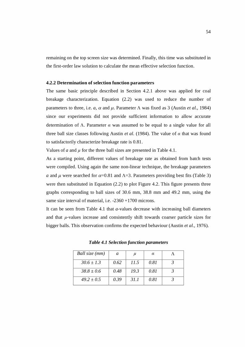
54

remaining on the top screen size was determined. Finally, this time was substituted in

the first-order law solution to calculate the mean effective selection function.

4.2.2 Determination of selection function parameters

The same basic principle described in Section 4.2.1 above was applied for coal

breakage characterization. Equation (2.2) was used to reduce the number of

parameters to three, i.e. a, and . Parameter was fixed as 3 (Austin et al., 1984)

since our experiments did not provide sufficient information to allow accurate

determination of . Parameter α was assumed to be equal to a single value for all

three ball size classes following Austin et al. (1984). The value of α that was found

to satisfactorily characterize breakage rate is 0.81.

Values of a and µ for the three ball sizes are presented in Table 4.1.

As a starting point, different values of breakage rate as obtained from batch tests

were compiled. Using again the same non-linear technique, the breakage parameters

a and were searched for =0.81 and =3. Parameters providing best fits (Table 3)

were then substituted in Equation (2.2) to plot Figure 4.2. This figure presents three

graphs corresponding to ball sizes of 30.6 mm, 38.8 mm and 49.2 mm, using the

same size interval of material, i.e. -2360 +1700 microns.

It can be seen from Table 4.1 that a-values decrease with increasing ball diameters

and that µ-values increase and consistently shift towards coarser particle sizes for

bigger balls. This observation confirms the expected behaviour (Austin et al., 1976).

Table 4.1 Selection function parameters

Ball size (mm) a µ α

30.6 ± 1.3 0.62 11.5 0.81 3

38.8 ± 0.6 0.48 19.3 0.81 3

49.2 ± 0.5 0.39 31.1 0.81 3

55

4.3 Effect of ball size

4.3.1 Breakage rate as a function of ball size

To study the effect of ball diameter on the selection function, Equations (2.10) and

(2.11) are used. In these two equations, the factor relates a-values to the ball size

while the factor does the same between µ-values and the ball size.

Considering the values in Table 4.1, a parameter search was implemented on to

define the relationship a-versus-d. The value found was 1.07 ± 0.1 which confirms

the value of 1 proposed by Austin et al. (1984).

Similarly, the factor was searched for. This time, was found to be 2.08 ± 0.1.

The point to make here is that the value of =2 has been proposed by Kelsall et al.

(1967) and then confirmed by Austin et al. (1976), which implies a surface wear

mechanism. Recently, many values have been reported and it is still unclear what

might be the reason for these diverging findings (Yildirim et al., 1999; Kotake et al.,

2004; Austin et al., 2006).

Figure 4.2 Effect of ball diameter on the selection function

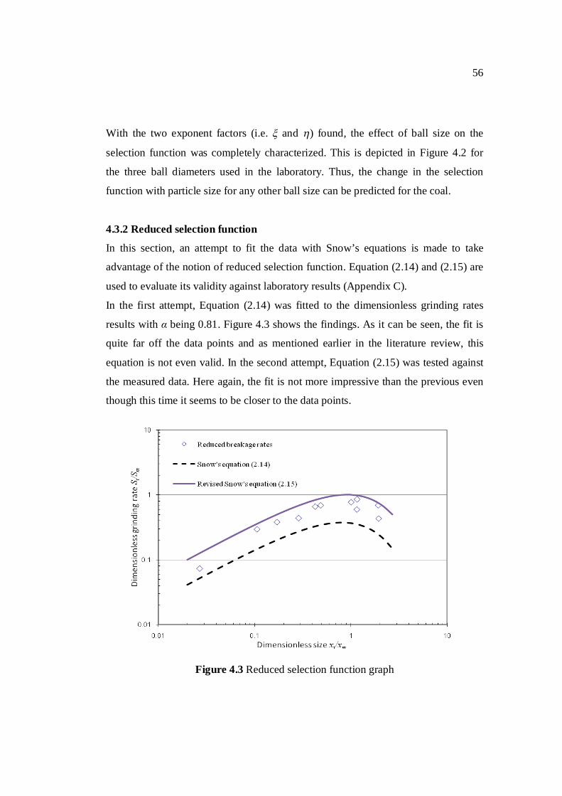
56

With the two exponent factors (i.e. and ) found, the effect of ball size on the

selection function was completely characterized. This is depicted in Figure 4.2 for

the three ball diameters used in the laboratory. Thus, the change in the selection

function with particle size for any other ball size can be predicted for the coal.

4.3.2 Reduced selection function

In this section, an attempt to fit the data with Snow’s equations is made to take

advantage of the notion of reduced selection function. Equation (2.14) and (2.15) are

used to evaluate its validity against laboratory results (Appendix C).

In the first attempt, Equation (2.14) was fitted to the dimensionless grinding rates

results with α being 0.81. Figure 4.3 shows the findings. As it can be seen, the fit is

quite far off the data points and as mentioned earlier in the literature review, this

equation is not even valid. In the second attempt, Equation (2.15) was tested against

the measured data. Here again, the fit is not more impressive than the previous even

though this time it seems to be closer to the data points.

Figure 4.3 Reduced selection function graph

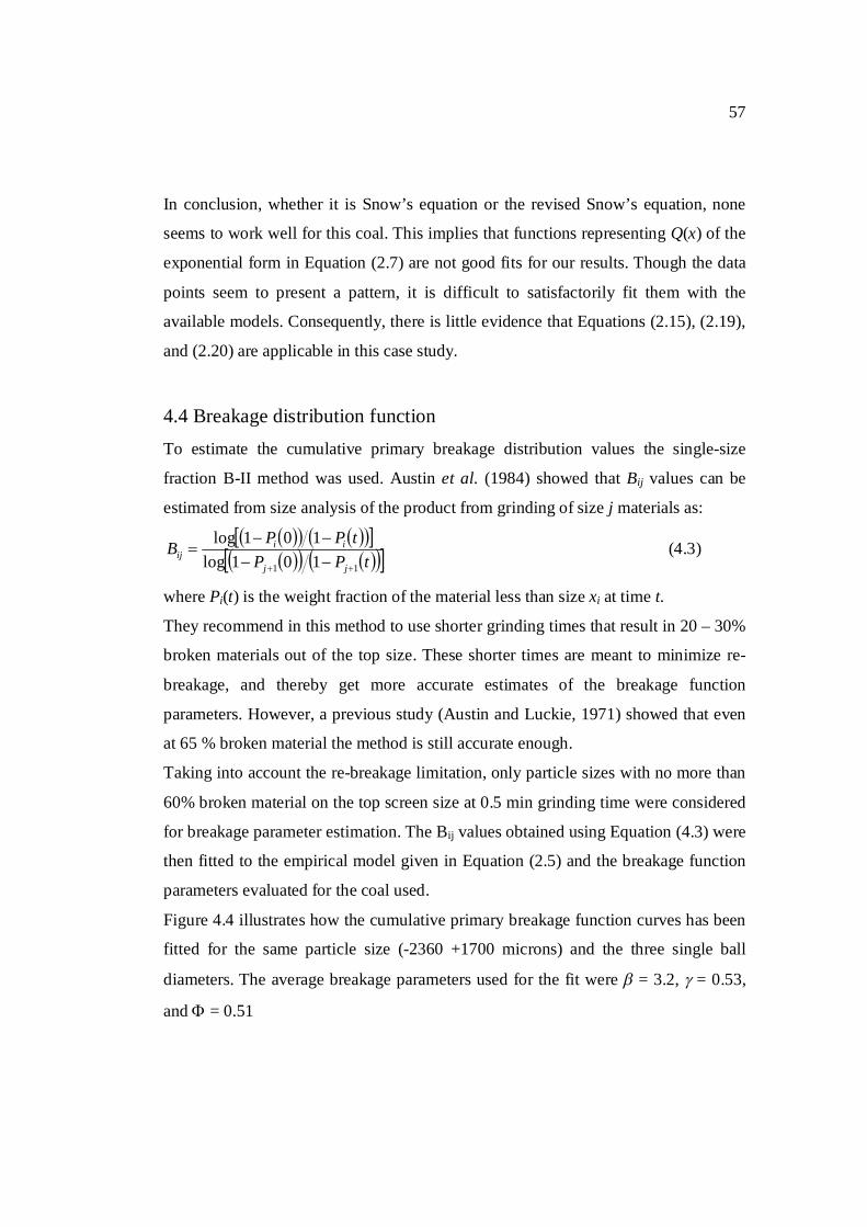
57

In conclusion, whether it is Snow’s equation or the revised Snow’s equation, none

seems to work well for this coal. This implies that functions representing Q(x) of the

exponential form in Equation (2.7) are not good fits for our results. Though the data

points seem to present a pattern, it is difficult to satisfactorily fit them with the

available models. Consequently, there is little evidence that Equations (2.15), (2.19),

and (2.20) are applicable in this case study.

4.4 Breakage distribution function To estimate the cumulative primary breakage distribution values the single-size

fraction B-II method was used. Austin et al. (1984) showed that Bij values can be

estimated from size analysis of the product from grinding of size j materials as:

tPP

tPPBjj

iiij

11 101log101log

(4.3)

where Pi(t) is the weight fraction of the material less than size xi at time t.

They recommend in this method to use shorter grinding times that result in 20 – 30%

broken materials out of the top size. These shorter times are meant to minimize re-

breakage, and thereby get more accurate estimates of the breakage function

parameters. However, a previous study (Austin and Luckie, 1971) showed that even

at 65 % broken material the method is still accurate enough.

Taking into account the re-breakage limitation, only particle sizes with no more than

60% broken material on the top screen size at 0.5 min grinding time were considered

for breakage parameter estimation. The Bij values obtained using Equation (4.3) were

then fitted to the empirical model given in Equation (2.5) and the breakage function

parameters evaluated for the coal used.

Figure 4.4 illustrates how the cumulative primary breakage function curves has been

fitted for the same particle size (-2360 +1700 microns) and the three single ball

diameters. The average breakage parameters used for the fit were = 3.2, = 0.53,

and = 0.51

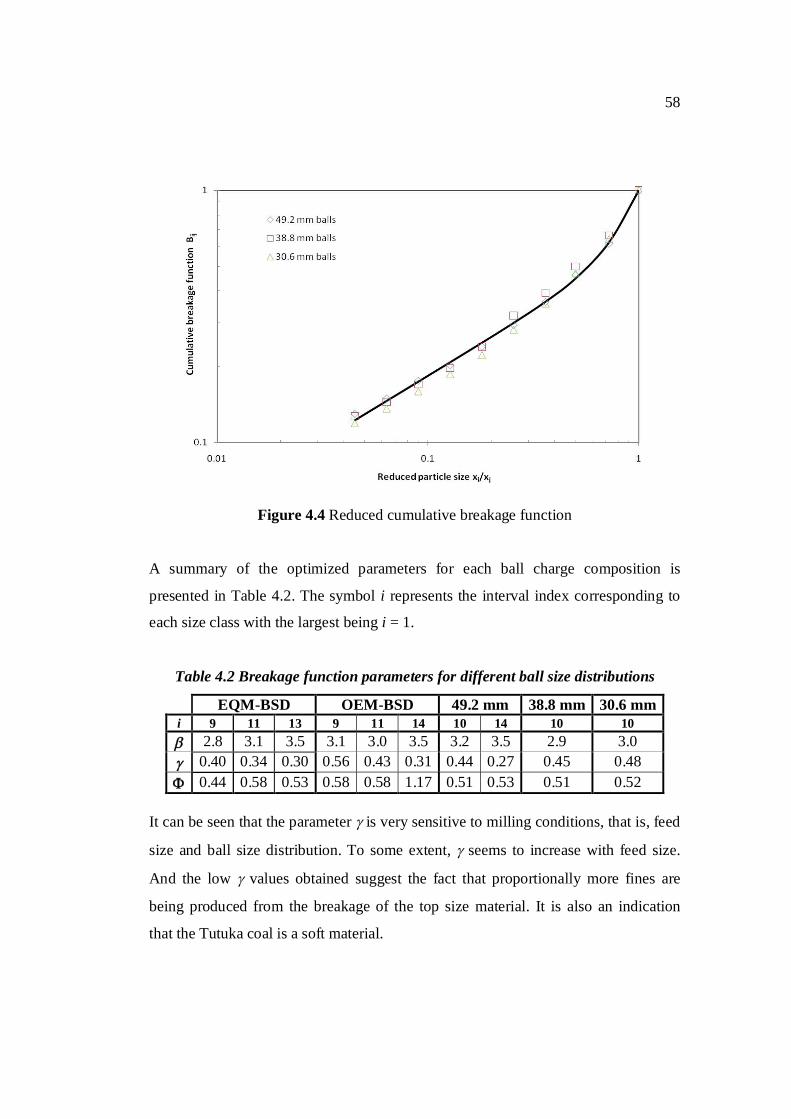
58

Figure 4.4 Reduced cumulative breakage function

A summary of the optimized parameters for each ball charge composition is

presented in Table 4.2. The symbol i represents the interval index corresponding to

each size class with the largest being i = 1.

Table 4.2 Breakage function parameters for different ball size distributions

EQM-BSD OEM-BSD 49.2 mm 38.8 mm 30.6 mm i 9 11 13 9 11 14 10 14 10 10 2.8 3.1 3.5 3.1 3.0 3.5 3.2 3.5 2.9 3.0 0.40 0.34 0.30 0.56 0.43 0.31 0.44 0.27 0.45 0.48 0.44 0.58 0.53 0.58 0.58 1.17 0.51 0.53 0.51 0.52

It can be seen that the parameter is very sensitive to milling conditions, that is, feed

size and ball size distribution. To some extent, seems to increase with feed size.

And the low values obtained suggest the fact that proportionally more fines are

being produced from the breakage of the top size material. It is also an indication

that the Tutuka coal is a soft material.

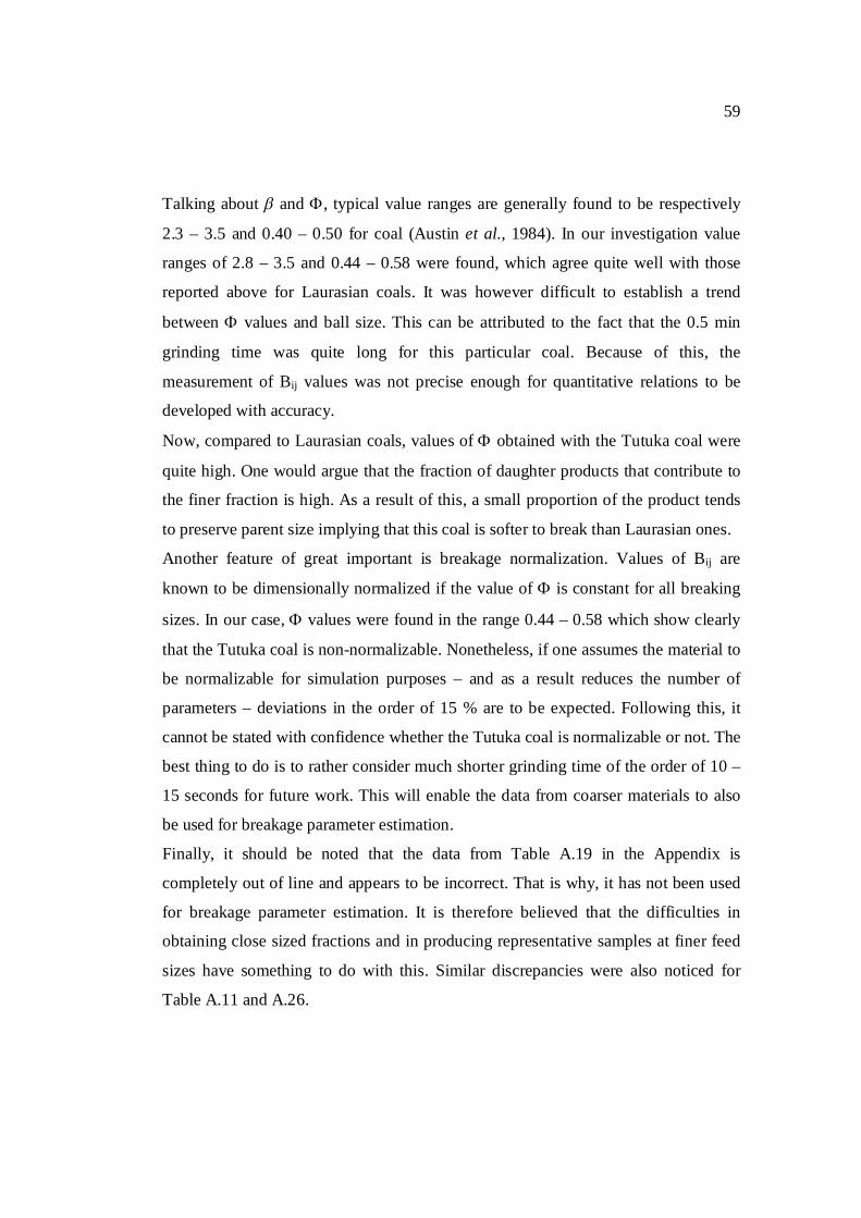
59

Talking about and , typical value ranges are generally found to be respectively

2.3 – 3.5 and 0.40 – 0.50 for coal (Austin et al., 1984). In our investigation value

ranges of 2.8 – 3.5 and 0.44 – 0.58 were found, which agree quite well with those

reported above for Laurasian coals. It was however difficult to establish a trend

between values and ball size. This can be attributed to the fact that the 0.5 min

grinding time was quite long for this particular coal. Because of this, the

measurement of Bij values was not precise enough for quantitative relations to be

developed with accuracy.

Now, compared to Laurasian coals, values of obtained with the Tutuka coal were

quite high. One would argue that the fraction of daughter products that contribute to

the finer fraction is high. As a result of this, a small proportion of the product tends

to preserve parent size implying that this coal is softer to break than Laurasian ones.

Another feature of great important is breakage normalization. Values of Bij are

known to be dimensionally normalized if the value of is constant for all breaking

sizes. In our case, values were found in the range 0.44 – 0.58 which show clearly

that the Tutuka coal is non-normalizable. Nonetheless, if one assumes the material to

be normalizable for simulation purposes – and as a result reduces the number of

parameters – deviations in the order of 15 % are to be expected. Following this, it

cannot be stated with confidence whether the Tutuka coal is normalizable or not. The

best thing to do is to rather consider much shorter grinding time of the order of 10 –

15 seconds for future work. This will enable the data from coarser materials to also

be used for breakage parameter estimation.

Finally, it should be noted that the data from Table A.19 in the Appendix is

completely out of line and appears to be incorrect. That is why, it has not been used

for breakage parameter estimation. It is therefore believed that the difficulties in

obtaining close sized fractions and in producing representative samples at finer feed

sizes have something to do with this. Similar discrepancies were also noticed for

Table A.11 and A.26.

60

4.5 Significance of results (Interpretation) The dependency of a-values on ball diameter d is best described using Equation (10)

in which =1 as presented in literature (Austin et al., 1984). But earlier laws defined

the competent media as the size of the ball corresponding to the maximum rate of

breakage for a given size of particle. The following empirical equation was used: dKxm . (4.4)

This equation is generalized based upon Equations (2.9) and (2.11) in which α, , a0,

µ0, and d0 are constant. Moreover, Equation (2.9) shows that xm is directly

proportional to making no difference in the use of xm in lieu of in the analysis.

Austin et al. (1976) reported that the competent ball size was determined using

Equation (4.4) in which =2. Interestingly, the value of was found to be 2 for the

Tutuka coal.

Kelsall et al. (1967) proposed =2 based on experiments done on quartz material.

They reported in fact that this exponent was used for decades as an empirical way of

choosing the competent ball diameter. Austin et al. (1984) also found a value of 2

based on experiment they did on coal.

Yildirim et al. (1999) in their particular case found that =1 simulated reasonably

well a dry grinding circuit of quartz. Recently, Austin et al. (2006) substituted 1.2 for

on an iron ore.

On their side, Kotake et al. (2004) were able to show that is relatively larger for

synthesized silica glass than for other materials they used. On average, they reported

values between 0.89 and 1.42. The most important point is that they believed these

discrepancies could be a result of inherent properties of the materials used such as

density, Mohs hardness, Vicker’s hardness, Young’s modulus, and Poisson’s ratio.

61

This suggests that the exponent factor is clearly not a predefined constant

parameter. It might primarily depend on the material used. For this reason, it is

justifiable to estimate it depending on the laboratory conditions.

Ultimately, no straightforward reason can be given to elucidate the different -values

reported. But it seems to us that this exponent factor is material-dependent. Only a

detailed and systematic investigation will tell more on this hypothesis.

4.6 Summary Equation (2.7) works very well providing the correction factor is given by Equation

(2.8). Conversely, Equation (2.15) seems not to work at all here. Austin et al. (1986)

also reached the same conclusion.

As far as the selection function equation is concerned, Equation (2.8) is entirely

adequate as correction factor and seems to be the best model for the limited amount

of information available at hand.

As for the breakage function, it has revealed the material to be non-normalizable.

However, within 15 % deviation, the Tutuka coal can still be considered

normalizable. And until more information is made available, not much can be done

as to modelling the breakage function. At least, at this point in time, the proportional

variation of and presented in Table 4.2 can be used in preliminary simulations.

But one needs to bear in mind that for qualitative works, complex models may be

required especially with naturally-occurring minerals like the coal under

consideration. This can be possible only when a well-thought laboratory work plan

intended towards measuring the breakage function parameters is devised.

More importantly, published values of so far range between 1 and 2. With the high

value of the factor found in this case study, the ball size effect reveals that this coal

will be very sensitive to the ball size distribution inside the mill. Such an anticipated

statement is evaluated in the next chapter.

62

Chapter 5 Effect of ball size distribution on milling kinetics

Single sizes of balls used for breakage parameter estimation do not represent at all

the ball size distribution of an industrial mill even at start-up. For that reason, true

validation of the milling process comes from the tests that mimic a real ball mixture.

For that reason, two ball size distributions were tested and the results obtained

compared to the prediction using appropriate models.

In this chapter, raw data corresponding to two ball mixtures are manipulated in order

to get a reasonable description of the effect of ball size distribution on breakage rate

of a South African coal. This information can in future be used in the scale-up of

laboratory results or simulated behaviour of various ball mixtures for industrial

applications.

5.1 Introduction The choice of media charge composition that optimizes ball milling circuits has had

significant financial implications. This problem has been industrially addressed using

a trial-and-error approach coupled with experience. Mill performance and ball size

distribution are so intimately related that it is crucial to better understand their

interrelation. This will then orientate process engineers in choosing the optimal ball

mixture.

For the first time, Concha et al. (1992) proposed a remarkable algorithm that can be

used to optimize the ball charge composition under defined operating constraints.

This method relies on batch laboratory tests. These tests are used to characterize the

grinding properties of the material being studied. The amount of laboratory work

required to fully characterize the mineral matter is considerable. Tests are lengthy,

tedious, and physically-challenging. Additionally, batch tests are carried out on

several narrow particle size classes using single ball sizes. To have an estimate of the

63

overall effect of a mixture of balls in the mill, one must measure it on a well defined

ball size distribution. In latter case, the data obtained will be valid for the considered

ball mixture which should be similar to that used in the industrial mill. At present, no

model is available that fully predicts the behaviour of a ball mix without relying

upon results of batch tests for single ball sizes.

Typically, at least three single ball sizes are needed to unambiguously model the

effect of ball diameter on milling rate. Then, a mix of balls can also be tested to

mimic for example a real ball size distribution of an industrial plant. This set of

information is then incorporated in the simulation model to obtain the optimum

charge composition.

The core of this chapter focuses on investigating the effect of ball size distribution on

the milling properties of the Tutuka coal. The sensitivity of the milling rate with the

ball size distribution is examined to get much insight on the dependence of breakage

rate of coal on the ball size distribution.

5.2 Selection function of ball mixtures Milling rates are investigated for two charge mixes. Then, the measured rates are

compared to the predicted ones. Finally, the discrepancies are discussed.

5.2.1 Equilibrium ball size distribution

Equation (2.30) shows that the equilibrium charge consists of an equal number of

balls in each ball class providing the class widths are the same. In other words,

according to Bond law, the equilibrium ball charge distribution is in statistical terms

a constant number distribution function. This property was used to prepare the first

charge mass denoted here EQM-BSD. Distributions in terms of mass and number

fractions are presented in Figures 5.1 and 5.2 along with the second ball charge

which will be discussed in the next sub-section.

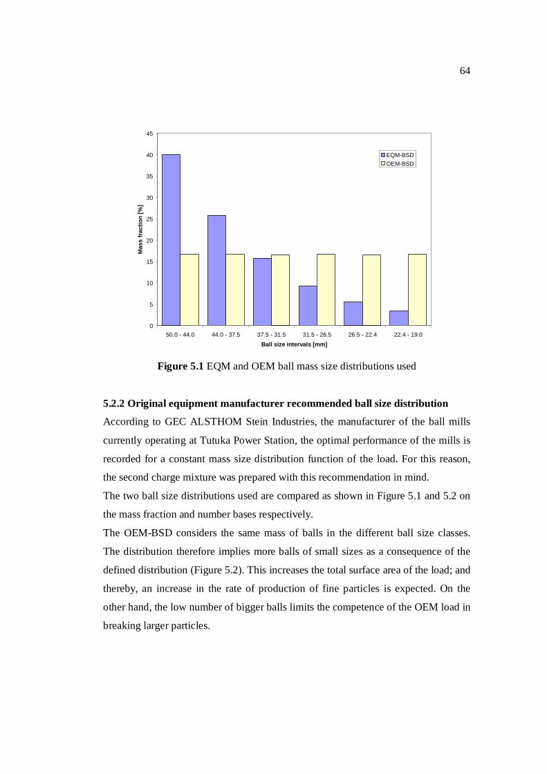
64

0

5

10

15

20

25

30

35

40

45

50.0 - 44.0 44.0 - 37.5 37.5 - 31.5 31.5 - 26.5 26.5 - 22.4 22.4 - 19.0Ball size intervals [mm]

Mas

s fr

actio

n [%

]

EQM-BSDOEM-BSD

Figure 5.1 EQM and OEM ball mass size distributions used

5.2.2 Original equipment manufacturer recommended ball size distribution

According to GEC ALSTHOM Stein Industries, the manufacturer of the ball mills

currently operating at Tutuka Power Station, the optimal performance of the mills is

recorded for a constant mass size distribution function of the load. For this reason,

the second charge mixture was prepared with this recommendation in mind.

The two ball size distributions used are compared as shown in Figure 5.1 and 5.2 on

the mass fraction and number bases respectively.

The OEM-BSD considers the same mass of balls in the different ball size classes.

The distribution therefore implies more balls of small sizes as a consequence of the

defined distribution (Figure 5.2). This increases the total surface area of the load; and

thereby, an increase in the rate of production of fine particles is expected. On the

other hand, the low number of bigger balls limits the competence of the OEM load in

breaking larger particles.

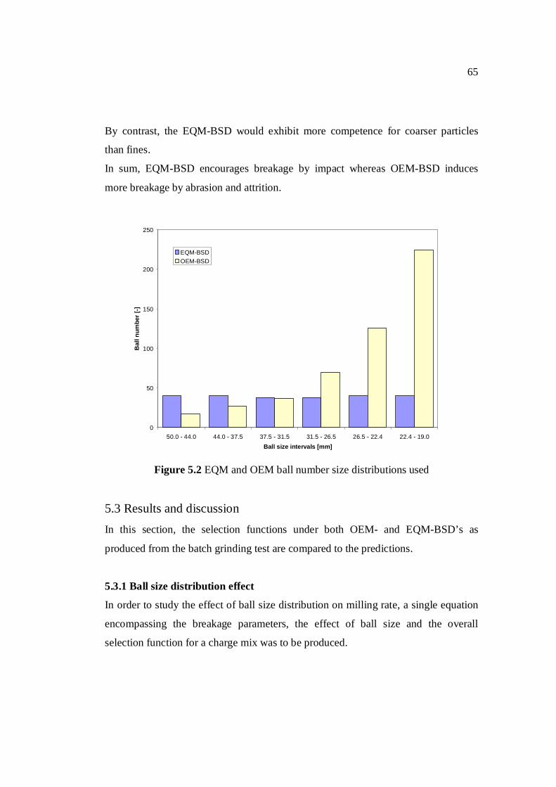
65

By contrast, the EQM-BSD would exhibit more competence for coarser particles

than fines.

In sum, EQM-BSD encourages breakage by impact whereas OEM-BSD induces

more breakage by abrasion and attrition.

0

50

100

150

200

250

50.0 - 44.0 44.0 - 37.5 37.5 - 31.5 31.5 - 26.5 26.5 - 22.4 22.4 - 19.0Ball size intervals [mm]

Bal

l num

ber

[-]

EQM-BSDOEM-BSD

Figure 5.2 EQM and OEM ball number size distributions used

5.3 Results and discussion In this section, the selection functions under both OEM- and EQM-BSD’s as

produced from the batch grinding test are compared to the predictions.

5.3.1 Ball size distribution effect

In order to study the effect of ball size distribution on milling rate, a single equation

encompassing the breakage parameters, the effect of ball size and the overall

selection function for a charge mix was to be produced.

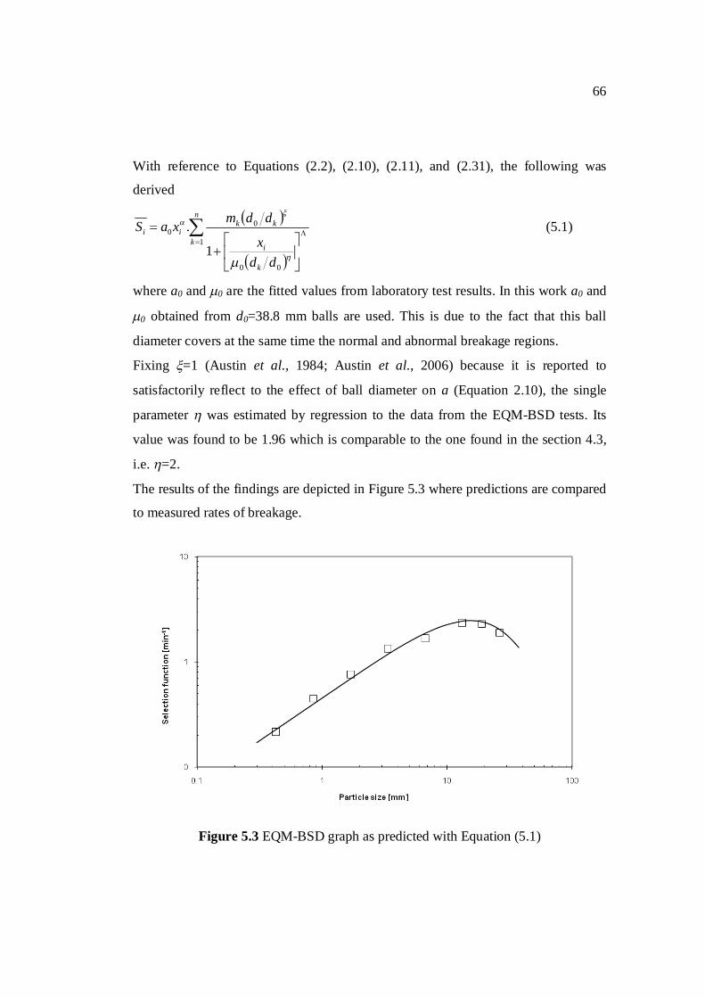
66

With reference to Equations (2.2), (2.10), (2.11), and (2.31), the following was

derived

n

k

k

i

kkii

ddx

ddmxaS1

00

00

1

.

(5.1)

where a0 and 0 are the fitted values from laboratory test results. In this work a0 and

0 obtained from d0=38.8 mm balls are used. This is due to the fact that this ball

diameter covers at the same time the normal and abnormal breakage regions.

Fixing =1 (Austin et al., 1984; Austin et al., 2006) because it is reported to

satisfactorily reflect to the effect of ball diameter on a (Equation 2.10), the single

parameter was estimated by regression to the data from the EQM-BSD tests. Its

value was found to be 1.96 which is comparable to the one found in the section 4.3,

i.e. =2.

The results of the findings are depicted in Figure 5.3 where predictions are compared

to measured rates of breakage.

Figure 5.3 EQM-BSD graph as predicted with Equation (5.1)

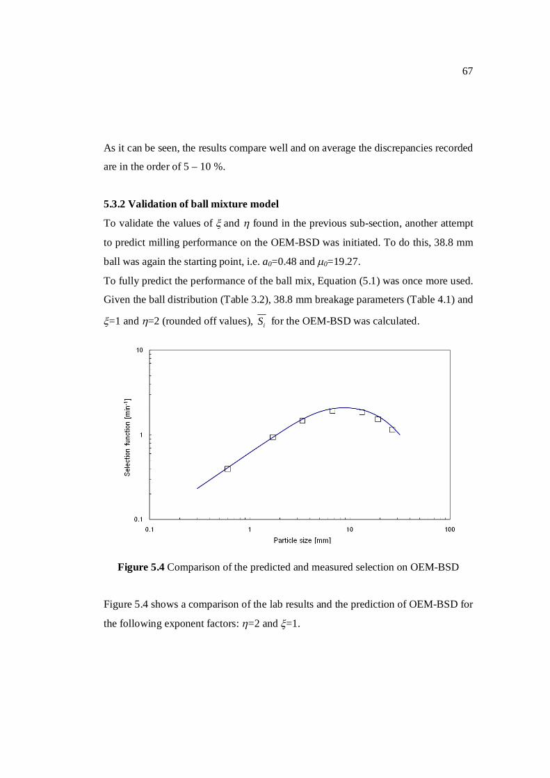
67

As it can be seen, the results compare well and on average the discrepancies recorded

are in the order of 5 – 10 %.

5.3.2 Validation of ball mixture model

To validate the values of and found in the previous sub-section, another attempt

to predict milling performance on the OEM-BSD was initiated. To do this, 38.8 mm

ball was again the starting point, i.e. a0=0.48 and 0=19.27.

To fully predict the performance of the ball mix, Equation (5.1) was once more used.

Given the ball distribution (Table 3.2), 38.8 mm breakage parameters (Table 4.1) and

=1 and =2 (rounded off values), iS for the OEM-BSD was calculated.

Figure 5.4 Comparison of the predicted and measured selection on OEM-BSD

Figure 5.4 shows a comparison of the lab results and the prediction of OEM-BSD for

the following exponent factors: =2 and =1.

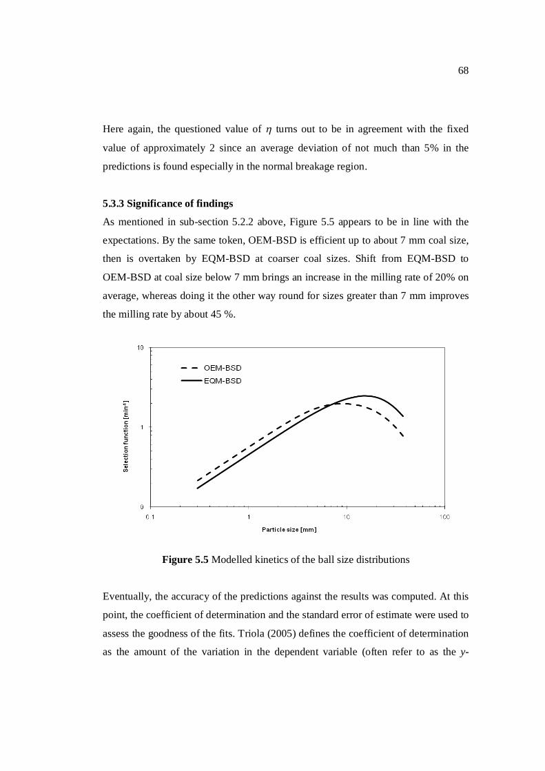
68

Here again, the questioned value of turns out to be in agreement with the fixed

value of approximately 2 since an average deviation of not much than 5% in the

predictions is found especially in the normal breakage region.

5.3.3 Significance of findings

As mentioned in sub-section 5.2.2 above, Figure 5.5 appears to be in line with the

expectations. By the same token, OEM-BSD is efficient up to about 7 mm coal size,

then is overtaken by EQM-BSD at coarser coal sizes. Shift from EQM-BSD to

OEM-BSD at coal size below 7 mm brings an increase in the milling rate of 20% on

average, whereas doing it the other way round for sizes greater than 7 mm improves

the milling rate by about 45 %.

Figure 5.5 Modelled kinetics of the ball size distributions

Eventually, the accuracy of the predictions against the results was computed. At this

point, the coefficient of determination and the standard error of estimate were used to

assess the goodness of the fits. Triola (2005) defines the coefficient of determination

as the amount of the variation in the dependent variable (often refer to as the y-

69

variable) that is explained by the regression line with respect to the predictor

variable. Known also as the R-squared value, it is a way of evaluating the quality of

a curve fit. As a rule of thumb, Palm (2001) recommends a value of r2 ≥ 0.99; in

other words, a fit is good if it accounts for at least 99 % of the data variation.

However, for practical applications, Triola (2005) argues that a value of r2 ≥ 0.95 is

the standard accepted by statisticians worldwide.

In discussing this matter further, the definition given by Triola (2005) would be a

good starting point.

For a collection of paired data containing of sample points (x,y), if ymdl is defined as

the predicted value of y (obtained by using the regression equation), and y as the

mean of the sample y-values, the following can be deduced:

1° The explained deviation is the vertical distance ymdl – y , which is the distance

between the predicted y-value and the horizontal line passing through the

sample mean y .

2° The unexplained deviation is the vertical distance y – ymdl, which is the vertical

distance between the point (x,y) and the regression line. This distance y – ymdl

is also called residual.

3° The total deviation (from the mean) of the particular point (x,y) is the vertical

distance y – y , which is the distance between the point (x, y) and the horizontal

line passing through the sample mean y .

With reference to the above, the coefficient of determination is defined as

variationTotal variationExplained2 r (5.2)

where the total variation represents the sum of the squares of the total deviation

values and the explained variation is the sum of the squares of the explained

deviation values.

In order to determine the accuracy of a predicted value, the notion of prediction

interval is brought up, which is an interval estimate of a predicted value of y. From

70

there, the spread of sample points about the regression line and the average error of

estimate can be calculated.

The standard error of estimate, denoted by se, represents a measure of the differences

(or distances) between the observed sample y-values and the predicted values ymdl

that are obtained using the regression equation. It is given by (Triola, 2005)

2

2

Nyy

s mdle (5.3)

where ymdl is the predicted y-value and N is the number of sample points.

In this case study, it was found that:

- For the EQM-BSD, r2=0.977 and the average error of estimate was 9.18 %

- and for the OEM-BSD, r2=0.986 and the average error of estimate was 4.89 %.

Though high coefficients of determination are found, they cannot provide good

answers to the underlying engineering or scientific questions under investigation.

Nevertheless Equation (5.1) approximates the measured data points very well.

5.4 Summary Two ball charge mixtures were compared. It was found as expected that on the one

hand the selection function graph corresponding to the EQM-BSD lies below the

OEM-BSD one at lower particle sizes; and on the other hand, it increases

continuously and becomes higher for coarser sizes.

Equation (5.1) which gives an estimate of the overall value of breakage rate for a ball

mixture in the mill accurately describes the ball size distribution effect. With (the

factor which relates a to d) and (the factor which relates µ to d) estimated in the

previous chapter to be respectively 1 and 2, the selection function for the ball size

mixture can be reasonably predicted with an average deviation of 5 – 10 %.

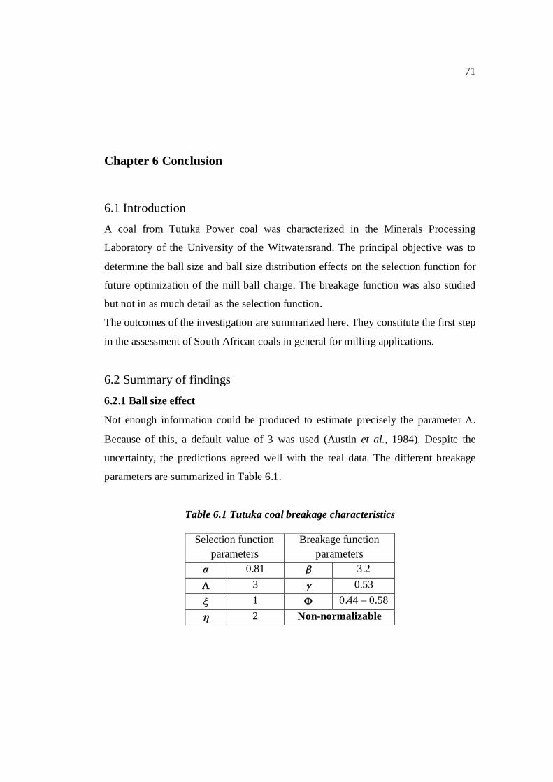
71

Chapter 6 Conclusion

6.1 Introduction A coal from Tutuka Power coal was characterized in the Minerals Processing

Laboratory of the University of the Witwatersrand. The principal objective was to

determine the ball size and ball size distribution effects on the selection function for

future optimization of the mill ball charge. The breakage function was also studied

but not in as much detail as the selection function.

The outcomes of the investigation are summarized here. They constitute the first step

in the assessment of South African coals in general for milling applications.

6.2 Summary of findings 6.2.1 Ball size effect

Not enough information could be produced to estimate precisely the parameter .

Because of this, a default value of 3 was used (Austin et al., 1984). Despite the

uncertainty, the predictions agreed well with the real data. The different breakage

parameters are summarized in Table 6.1.

Table 6.1 Tutuka coal breakage characteristics

Selection function parameters

Breakage function parameters

α 0.81 3.2 3 0.53 1 0.44 – 0.58 2 Non-normalizable

72

Even though the primary breakage distribution function was not studied in much

detail, the preliminary calculations suggested that the coal could be considered non-

normalizable. A more elaborated laboratory work plan intended towards measuring

accurately the breakage function parameters is required in future. Until this work is

systematically carried out, estimations given in Table 6.1 will be used as such for

preliminary simulations.

As for the breakage function parameters, the low value of is an indication that the

Tutuka coal is a very soft material.

On another note, Equations (2.14) and (2.15) were tried out. In spite of the fact that

the laboratory results seems to display a trend, Snow’s equations could not fit the

data well. To a large extent, Snow’s equations (2.14) and (2.15) do not approximate

at all the selection function values measured.

6.2.2 Ball size distribution effect

This study has revealed that an increase of 20 – 45 % in the selection function is

achievable by increasing the proportion of small balls in the mill charge. It has also

shown that South African coals are very sensitive to the ball charge mix. Therefore,

the optimization of the ball mix by simulation will always require confidence in the

model parameters to input to the simulator. Also observed, the overall breakage rate

due to a ball size mixture can be predicted from tests on a few individual ball sizes.

6.3 Overall conclusion The breakage properties of a South African coal were estimated and the effect of ball

size and ball size distribution deduced. An equation encompassing at the same time

ball size and ball size distribution effects for parameter search was tested. It was

found that the equation can be used for parameter estimation of the breakage

properties of materials.

In the final analysis, it was noted in particular that (the factor which relates a to d)

proves to be close to 1. The factor (the factor which relates µ to d), on the other

73

hand, is ostensibly material dependent. But the -value of 2 satisfactorily simulates

the behaviour of coal. Fixing a priori the value of is therefore inadequate. It should

rather be deduced from tests on at least two ball sizes which are substantially

different, e.g. 30 and 50 mm. As to whether parameter is material dependent or

not, only future research will tell. This will require more tests in the abnormal region

to confidently estimate the parameter .

74

References

Austin, L.G., Bagga, P., Celik, M., 1981. Breakage properties of some materials in a

laboratory ball mill, Powder Technology, vol. 28, no. 2, pp. 235 – 241

Austin, L.G., Bhatia, V.K., 1971/72. Experimental methods for grinding studies in

laboratory mills, Powder Technology, vol. 5, no. 5, pp 261 – 266

Austin, L.G., Brame, K., 1983. A comparison of Bond method for sizing wet

tumbling ball mills with a size-mass balance simulation model, Powder Technology,

vol. 34, no. 2, pp. 261 – 274

Austin, L.G., Julianelli, K., de Souza, A.S., Schneider, C.L., 2006. Simulation of wet

ball milling of iron ore at Carajas – Brazil, International Journal of Mineral

Processing, vol. 84, no. 1 – 4, pp. 157 – 171

Austin, L.G., Klimpel, R.R., 1985. Ball wear and ball size distribution in tumbling

mills, Powder Technology, vol. 41, no. 3, pp. 279 – 286

Austin, L.G., Klimpel, R.R., Luckie, P.T., 1984. Process Engineering of Size

Reduction: Ball Milling, AIME-SME, New York, USA

75

Austin, L.G., Luckie, P.T., 1971/72. Methods for determination of breakage

distribution parameters, Powder Technology, vol. 5, no. 4, pp 215 – 222

Austin, L.G., Shoji, K., Everett, M.D., 1973. An explanation of abnormal breakage

of large particle sizes in laboratory mills, Powder Technology, vol. 7, no. 1, pp 3 – 7

Austin, L.G., Shoji, K., Bell, D., 1982. Rate equations for non-linear breakage in

mills due to material effects, Powder Technology, vol. 31, no. 1, pp. 127 – 133

Austin, L.G., Shoji, K., Luckie, P.T., 1976. The effect of ball size on mill

performance, Powder Technology, vol. 14, no. 1, pp. 71 – 79

Austin, L.G., Trimarchi, T., Weymont, N.P., 1977. An analysis of some cases of

non-first-order breakage rates, Powder Technology, vol. 17, no. 1, pp. 109 – 113

Bazin, C., 2005. Data reconciliation for the calibration of a model for batch grinding,

Minerals Engineering, vol. 18, no. 10, pp. 1052 – 1056

Cleary, P.W., 2001. Charge behaviour and power consumption in ball mills:

sensitivity to mill operating conditions, liner geometry and charge composition,

International Journal of Mineral Processing, vol. 63, no. 2, pp. 79 – 114

76

Concha, F., Magne, L., Austin, L.G., 1992. Optimization of the make-up ball charge

in a grinding mill, International Journal of Mineral Processing, vol. 34, no. 3, pp.

231 – 241

Falcon, L.M., Falcon, R.M.S., 1987. The petrographic composition of Southern

African coals in relation to friability, hardness, and abrasive indices, Journal of the

South African Institute of Mining and Metallurgy, vol. 87, no. 10, pp. 323 – 336

Falcon, R., Ham, A.J., 1988. The characteristics of Southern African coals, Journal

of the South African Institute of Mining and Metallurgy, vol. 88, no. 5, pp. 145 – 161

Gardner, R.P., Austin, L.G., 1975. The applicability of the first-order grinding law to

particles having a distribution of strengths, Powder Technology, vol. 12, no. 1, pp. 65

– 69

Gupta, A., Yan, D.S., 2006. Mineral Processing Design and Operation: An

introduction, Elsevier, ISBN: 978-0-4444-51636-7

Gupta, V.K., Zouit, H., Hodouin, D., 1985. The effect of ball and mill diameters on

grinding rate parameters in dry grinding operation, Powder Technology, vol. 42, no.

2, pp. 199 – 208

77

Hukki, R.T., 1954. Correlation between principal parameters affecting mechanical

ball wear, Mining Engineering, pp. 642 – 644

Kelly, E.G., Spottiswood, D.J., 1990. The breakage function; What is it really?,

Minerals Engineering, vol. 3, no. 5, pp. 405 – 414

Kelly, E.G., Spottiswood, D.J., 1982. Introduction to Mineral Processing, John Wiley

& Sons, ISBN 0-471-03379-0, USA.

Kelsall, D.F., Stewart, P.S.B., Weller, K.R., 1973. Continuous grinding in a small

wet ball mill. Part IV. A study of the influence of grinding media load and density,

Powder Technology, vol. 7, no. 5, pp. 293 – 301

Kelsall, D.F., Reid, K.J., Restarick, C.J., 1967. Continuous grinding in a small wet

ball mill. Part I. A study of the influence of ball diameter, Powder Technology, vol.

1, no. 5, pp. 291 – 300

King, R.P., 2001. Modeling and simulation of mineral processing systems,

Butterworth-Heinemann, ISBN: 0-7506-4884-8

78

Kotake, N., Daibo, K., Yamamoto, T., Kanda, Y., 2004. Experimental investigation

on a grinding rate constant of solid materials by a ball mill – effect of ball diameter

and feed size, Powder Technology, vol. 143 – 144, pp. 196 – 203

Kotake, N., Suzuki, K., Asahi, S., Kanda, Y., 2002. Experimental study on the

grinding rate constant of solid materials in a ball mill, Powder Technology, vol.122,

no. 2 – 3, pp. 101 – 108

Lameck, N.N.S., 2006. Coal selection and breakage functions parameterization,

Internal Report, University of the Witwatersrand, Johannesburg.

Lameck, N.N.S., 2006. Effects of grinding media shapes on ball mill performance,

Master of Science Dissertation, University of the Witwatersrand, Johannesburg.

Menacho, J., Concha, F., 1986. Mathematical model for ball wear in grinding mills,

I. Zero-order wear rate, Powder Technology, vol. 47, no. 1, pp. 87 – 96

Menacho, J., Concha, F., 1987. Mathematical model for ball wear in grinding mills,

II. General solution, Powder Technology, vol. 52, no. 3, pp. 267 – 277

79

Moys, M.H., 1984. The measurement of parameters describing behaviour of the load

in a grinding mill, Mintek 50, Proceedings of International Conference on Mineral

Science and Technology, Sandton, South Africa, pp. 205 – 219

Napier-Munn, T.J., Morrell, S., Morrison, R.D., Kojovic, T., 1999. Mineral

Comminution Circuits: Their Operation and Optimization. JKMRC, Queensland,

Australia

Nomura, S., Hosoda, K., Tanaka, T., 1991. An analysis of the selection function for

mills using balls as grinding media, Powder Technology, vol. 68, no.1, pp. 1 – 12

Nomura, S., Tanaka, T., Callcott, T.G., 1994. The effect of mill power on the

selection function for tumbling and vibration ball mills, Powder Technology, vol. 81,

no.2, pp. 101 – 109

Palm, W.J., 2001. Introduction to Matlab 6 for Engineers, McGraw-Hill, Boston,

USA

Powell, M.S., Morrison, R.D., 2007. The future of comminution modeling,

International Journal of Mineral Processing, vol. 84, no. 1 – 4, pp. 228 – 239

80

Triola, M.F., 2005. Essentials of Statistics, Second Edition, Pearson Addison-

Wesley, ISBN: 0-201-77129-2

Vermeulen, L.A., 1986. A contribution to ‘Ball wear and ball size distribution in

tumbling mills’, Powder Technology, vol. 46, no. 2 – 3, pp. 281 – 285

Wills, B.A., 1992. Mineral Processing Technology: An Introduction to the Practical

Aspects of Ore Treatment and Mineral Recovery, Fifth Edition. Pergamon

Yildirim, K., Austin, L.G., 1998. The abrasive wear of cylindrical grinding wear,

Wear, vol. 218, no. 1, pp. 15 – 20

Yildirim, K., Cho, H., Austin, L.G., 1999. The modeling of dry grinding of quartz in

tumbling media mills, Powder Technology, vol. 105, no. 1 – 3, pp. 210 – 221

81

Appendices

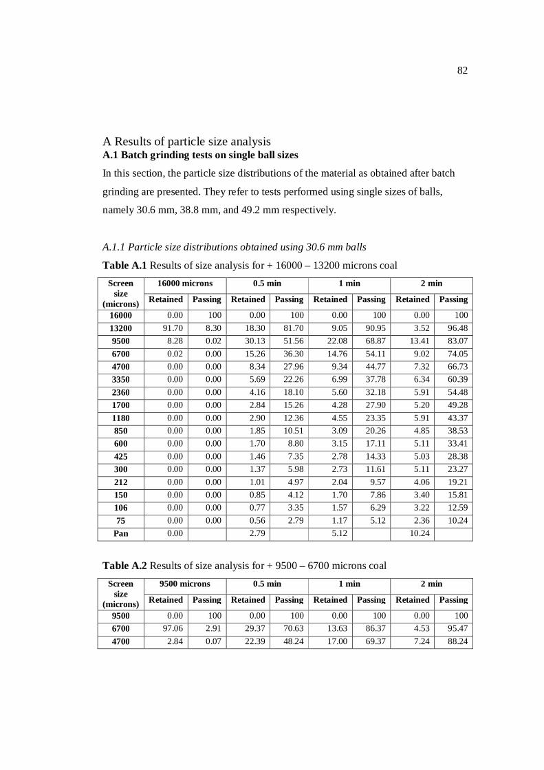
82

A Results of particle size analysis A.1 Batch grinding tests on single ball sizes

In this section, the particle size distributions of the material as obtained after batch

grinding are presented. They refer to tests performed using single sizes of balls,

namely 30.6 mm, 38.8 mm, and 49.2 mm respectively.

A.1.1 Particle size distributions obtained using 30.6 mm balls

Table A.1 Results of size analysis for + 16000 – 13200 microns coal Screen

size (microns)

16000 microns 0.5 min 1 min 2 min

Retained Passing Retained Passing Retained Passing Retained Passing

16000 0.00 100 0.00 100 0.00 100 0.00 100 13200 91.70 8.30 18.30 81.70 9.05 90.95 3.52 96.48 9500 8.28 0.02 30.13 51.56 22.08 68.87 13.41 83.07 6700 0.02 0.00 15.26 36.30 14.76 54.11 9.02 74.05 4700 0.00 0.00 8.34 27.96 9.34 44.77 7.32 66.73 3350 0.00 0.00 5.69 22.26 6.99 37.78 6.34 60.39 2360 0.00 0.00 4.16 18.10 5.60 32.18 5.91 54.48 1700 0.00 0.00 2.84 15.26 4.28 27.90 5.20 49.28 1180 0.00 0.00 2.90 12.36 4.55 23.35 5.91 43.37 850 0.00 0.00 1.85 10.51 3.09 20.26 4.85 38.53 600 0.00 0.00 1.70 8.80 3.15 17.11 5.11 33.41 425 0.00 0.00 1.46 7.35 2.78 14.33 5.03 28.38 300 0.00 0.00 1.37 5.98 2.73 11.61 5.11 23.27 212 0.00 0.00 1.01 4.97 2.04 9.57 4.06 19.21 150 0.00 0.00 0.85 4.12 1.70 7.86 3.40 15.81 106 0.00 0.00 0.77 3.35 1.57 6.29 3.22 12.59 75 0.00 0.00 0.56 2.79 1.17 5.12 2.36 10.24

Pan 0.00 2.79 5.12 10.24

Table A.2 Results of size analysis for + 9500 – 6700 microns coal

Screen size

(microns)



9500 0.00 100 0.00 100 0.00 100 0.00 100 6700 97.06 2.91 29.37 70.63 13.63 86.37 4.53 95.47 4700 2.84 0.07 22.39 48.24 17.00 69.37 7.24 88.24

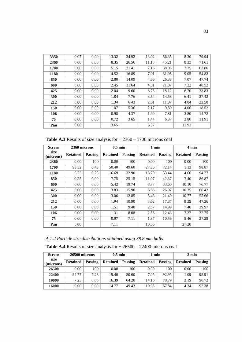
83

3350 0.07 0.00 13.32 34.92 13.02 56.35 8.30 79.94 2360 0.00 0.00 8.35 26.56 11.13 45.21 8.33 71.61 1700 0.00 0.00 5.15 21.41 7.16 38.05 7.75 63.86 1180 0.00 0.00 4.52 16.89 7.01 31.05 9.05 54.82 850 0.00 0.00 2.80 14.09 4.66 26.38 7.07 47.74 600 0.00 0.00 2.45 11.64 4.51 21.87 7.22 40.52 425 0.00 0.00 2.04 9.60 3.75 18.12 6.70 33.83 300 0.00 0.00 1.84 7.76 3.54 14.58 6.41 27.42 212 0.00 0.00 1.34 6.43 2.61 11.97 4.84 22.58 150 0.00 0.00 1.07 5.36 2.17 9.80 4.06 18.52 106 0.00 0.00 0.98 4.37 1.99 7.81 3.80 14.72 75 0.00 0.00 0.72 3.65 1.44 6.37 2.80 11.91

Pan 0.00 3.65 6.37 11.91


Screen size

(microns)



2360 0.00 100 0.00 100 0.00 100 0.00 100 1700 93.52 6.48 50.40 49.60 27.86 72.14 1.13 98.87 1180 6.23 0.25 16.69 32.90 18.70 53.44 4.60 94.27 850 0.25 0.00 7.75 25.15 11.07 42.37 7.40 86.87 600 0.00 0.00 5.42 19.74 8.77 33.60 10.10 76.77 425 0.00 0.00 3.83 15.90 6.63 26.97 10.35 66.42 300 0.00 0.00 3.06 12.85 5.48 21.49 10.77 55.66 212 0.00 0.00 1.94 10.90 3.62 17.87 8.29 47.36 150 0.00 0.00 1.51 9.40 2.87 14.99 7.40 39.97 106 0.00 0.00 1.31 8.08 2.56 12.43 7.22 32.75 75 0.00 0.00 0.97 7.11 1.87 10.56 5.46 27.28

Pan 0.00 7.11 10.56 27.28



Screen size

(microns)



26500 0.00 100 0.00 100 0.00 100 0.00 100 22400 92.77 7.23 19.40 80.60 7.05 92.95 1.09 98.91 19000 7.23 0.00 16.39 64.20 14.16 78.79 2.19 96.72 16000 0.00 0.00 14.77 49.43 10.95 67.84 4.34 92.38

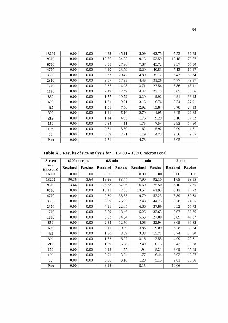
84

13200 0.00 0.00 4.32 45.11 5.09 62.75 5.53 86.85 9500 0.00 0.00 10.76 34.35 9.16 53.59 10.18 76.67 6700 0.00 0.00 6.38 27.98 7.87 45.72 9.37 67.30 4700 0.00 0.00 4.19 23.79 5.20 40.53 7.13 60.17 3350 0.00 0.00 3.37 20.42 4.80 35.72 6.43 53.74 2360 0.00 0.00 3.07 17.35 4.46 31.26 4.77 48.97 1700 0.00 0.00 2.37 14.98 3.71 27.54 5.86 43.11 1180 0.00 0.00 2.49 12.49 4.42 23.13 5.05 38.06 850 0.00 0.00 1.77 10.72 3.20 19.92 4.91 33.15 600 0.00 0.00 1.71 9.01 3.16 16.76 5.24 27.91 425 0.00 0.00 1.51 7.50 2.92 13.84 3.78 24.13 300 0.00 0.00 1.41 6.10 2.79 11.05 3.45 20.68 212 0.00 0.00 1.14 4.95 1.76 9.29 3.16 17.52 150 0.00 0.00 0.84 4.11 1.75 7.54 2.92 14.60 106 0.00 0.00 0.81 3.30 1.62 5.92 2.99 11.61 75 0.00 0.00 0.59 2.71 1.19 4.73 2.56 9.05

Pan 0.00 2.71 4.73 9.05


Screen size

(microns)



16000 0.00 100 0.00 100 0.00 100 0.00 100 13200 96.36 3.64 16.26 83.74 7.90 92.10 1.05 98.95 9500 3.64 0.00 25.78 57.96 16.60 75.50 6.10 92.85 6700 0.00 0.00 15.11 42.85 13.57 61.93 5.13 87.72 4700 0.00 0.00 9.30 33.55 9.70 52.23 6.89 80.83 3350 0.00 0.00 6.59 26.96 7.48 44.75 6.78 74.05 2360 0.00 0.00 4.91 22.05 6.86 37.89 8.32 65.73 1700 0.00 0.00 3.59 18.46 5.26 32.63 8.97 56.76 1180 0.00 0.00 3.62 14.84 5.63 27.00 8.89 47.87 850 0.00 0.00 2.34 12.50 4.06 22.94 8.05 39.82 600 0.00 0.00 2.11 10.39 3.85 19.09 6.28 33.54 425 0.00 0.00 1.80 8.59 3.38 15.71 5.74 27.80 300 0.00 0.00 1.62 6.97 3.16 12.55 4.99 22.81 212 0.00 0.00 1.29 5.68 2.40 10.15 3.43 19.38 150 0.00 0.00 0.93 4.75 1.94 8.21 3.69 15.69 106 0.00 0.00 0.91 3.84 1.77 6.44 3.02 12.67 75 0.00 0.00 0.66 3.18 1.29 5.15 2.61 10.06

Pan 0.00 3.18 5.15 10.06

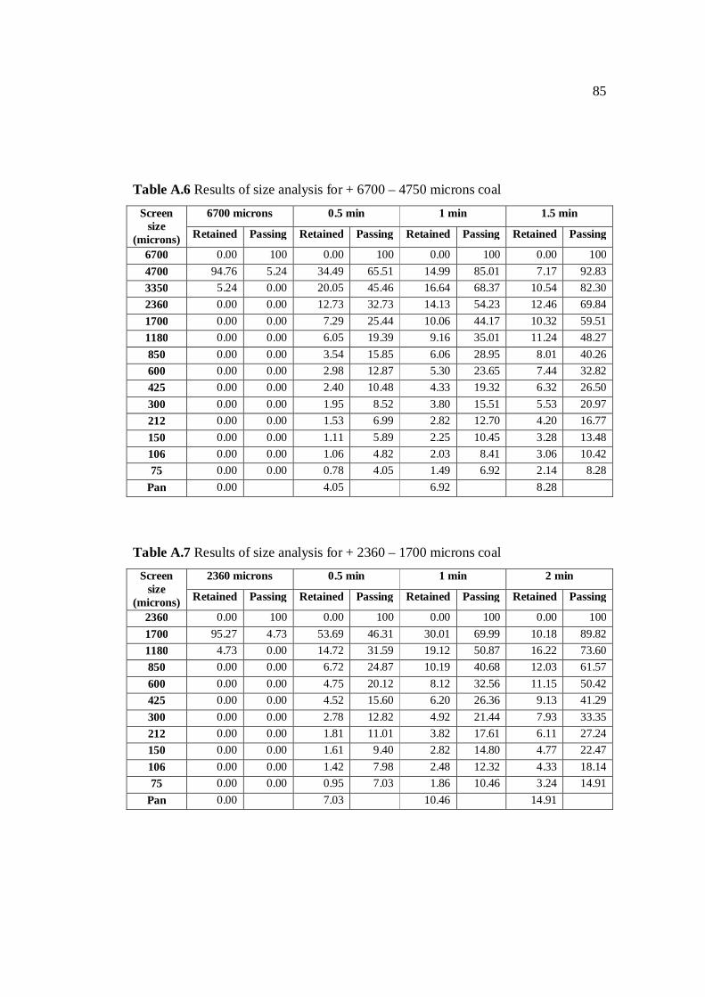
85


Screen size

(microns)

6700 microns 0.5 min 1 min 1.5 min


6700 0.00 100 0.00 100 0.00 100 0.00 100 4700 94.76 5.24 34.49 65.51 14.99 85.01 7.17 92.83 3350 5.24 0.00 20.05 45.46 16.64 68.37 10.54 82.30 2360 0.00 0.00 12.73 32.73 14.13 54.23 12.46 69.84 1700 0.00 0.00 7.29 25.44 10.06 44.17 10.32 59.51 1180 0.00 0.00 6.05 19.39 9.16 35.01 11.24 48.27 850 0.00 0.00 3.54 15.85 6.06 28.95 8.01 40.26 600 0.00 0.00 2.98 12.87 5.30 23.65 7.44 32.82 425 0.00 0.00 2.40 10.48 4.33 19.32 6.32 26.50 300 0.00 0.00 1.95 8.52 3.80 15.51 5.53 20.97 212 0.00 0.00 1.53 6.99 2.82 12.70 4.20 16.77 150 0.00 0.00 1.11 5.89 2.25 10.45 3.28 13.48 106 0.00 0.00 1.06 4.82 2.03 8.41 3.06 10.42 75 0.00 0.00 0.78 4.05 1.49 6.92 2.14 8.28

Pan 0.00 4.05 6.92 8.28


Screen size

(microns)



2360 0.00 100 0.00 100 0.00 100 0.00 100 1700 95.27 4.73 53.69 46.31 30.01 69.99 10.18 89.82 1180 4.73 0.00 14.72 31.59 19.12 50.87 16.22 73.60 850 0.00 0.00 6.72 24.87 10.19 40.68 12.03 61.57 600 0.00 0.00 4.75 20.12 8.12 32.56 11.15 50.42 425 0.00 0.00 4.52 15.60 6.20 26.36 9.13 41.29 300 0.00 0.00 2.78 12.82 4.92 21.44 7.93 33.35 212 0.00 0.00 1.81 11.01 3.82 17.61 6.11 27.24 150 0.00 0.00 1.61 9.40 2.82 14.80 4.77 22.47 106 0.00 0.00 1.42 7.98 2.48 12.32 4.33 18.14 75 0.00 0.00 0.95 7.03 1.86 10.46 3.24 14.91

Pan 0.00 7.03 10.46 14.91

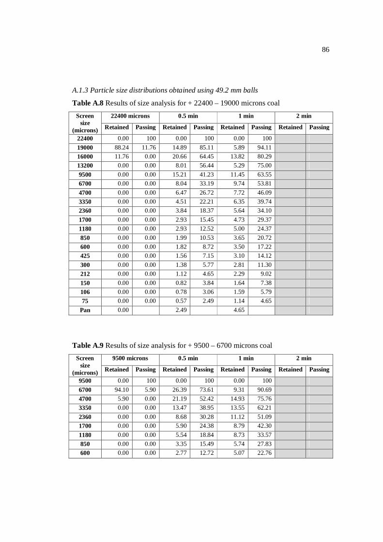
86



Screen size

(microns)



22400 0.00 100 0.00 100 0.00 100 19000 88.24 11.76 14.89 85.11 5.89 94.11 16000 11.76 0.00 20.66 64.45 13.82 80.29 13200 0.00 0.00 8.01 56.44 5.29 75.00 9500 0.00 0.00 15.21 41.23 11.45 63.55 6700 0.00 0.00 8.04 33.19 9.74 53.81 4700 0.00 0.00 6.47 26.72 7.72 46.09 3350 0.00 0.00 4.51 22.21 6.35 39.74 2360 0.00 0.00 3.84 18.37 5.64 34.10 1700 0.00 0.00 2.93 15.45 4.73 29.37 1180 0.00 0.00 2.93 12.52 5.00 24.37 850 0.00 0.00 1.99 10.53 3.65 20.72 600 0.00 0.00 1.82 8.72 3.50 17.22 425 0.00 0.00 1.56 7.15 3.10 14.12 300 0.00 0.00 1.38 5.77 2.81 11.30 212 0.00 0.00 1.12 4.65 2.29 9.02 150 0.00 0.00 0.82 3.84 1.64 7.38 106 0.00 0.00 0.78 3.06 1.59 5.79 75 0.00 0.00 0.57 2.49 1.14 4.65

Pan 0.00 2.49 4.65


Screen size

(microns)



9500 0.00 100 0.00 100 0.00 100 6700 94.10 5.90 26.39 73.61 9.31 90.69 4700 5.90 0.00 21.19 52.42 14.93 75.76 3350 0.00 0.00 13.47 38.95 13.55 62.21 2360 0.00 0.00 8.68 30.28 11.12 51.09 1700 0.00 0.00 5.90 24.38 8.79 42.30 1180 0.00 0.00 5.54 18.84 8.73 33.57 850 0.00 0.00 3.35 15.49 5.74 27.83 600 0.00 0.00 2.77 12.72 5.07 22.76

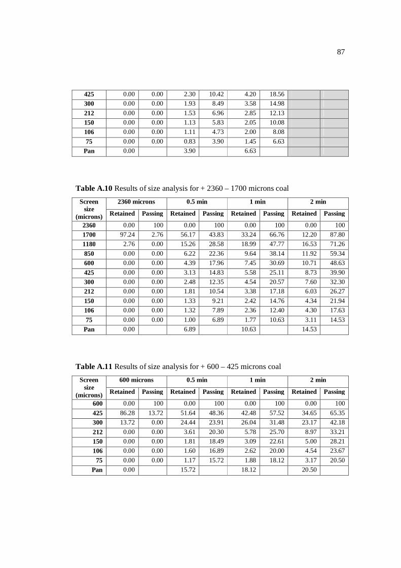
87

425 0.00 0.00 2.30 10.42 4.20 18.56 300 0.00 0.00 1.93 8.49 3.58 14.98 212 0.00 0.00 1.53 6.96 2.85 12.13 150 0.00 0.00 1.13 5.83 2.05 10.08 106 0.00 0.00 1.11 4.73 2.00 8.08 75 0.00 0.00 0.83 3.90 1.45 6.63

Pan 0.00 3.90 6.63


Screen size

(microns)



2360 0.00 100 0.00 100 0.00 100 0.00 100 1700 97.24 2.76 56.17 43.83 33.24 66.76 12.20 87.80 1180 2.76 0.00 15.26 28.58 18.99 47.77 16.53 71.26 850 0.00 0.00 6.22 22.36 9.64 38.14 11.92 59.34 600 0.00 0.00 4.39 17.96 7.45 30.69 10.71 48.63 425 0.00 0.00 3.13 14.83 5.58 25.11 8.73 39.90 300 0.00 0.00 2.48 12.35 4.54 20.57 7.60 32.30 212 0.00 0.00 1.81 10.54 3.38 17.18 6.03 26.27 150 0.00 0.00 1.33 9.21 2.42 14.76 4.34 21.94 106 0.00 0.00 1.32 7.89 2.36 12.40 4.30 17.63 75 0.00 0.00 1.00 6.89 1.77 10.63 3.11 14.53

Pan 0.00 6.89 10.63 14.53


Screen size

(microns)



600 0.00 100 0.00 100 0.00 100 0.00 100 425 86.28 13.72 51.64 48.36 42.48 57.52 34.65 65.35 300 13.72 0.00 24.44 23.91 26.04 31.48 23.17 42.18 212 0.00 0.00 3.61 20.30 5.78 25.70 8.97 33.21 150 0.00 0.00 1.81 18.49 3.09 22.61 5.00 28.21 106 0.00 0.00 1.60 16.89 2.62 20.00 4.54 23.67 75 0.00 0.00 1.17 15.72 1.88 18.12 3.17 20.50

Pan 0.00 15.72 18.12 20.50

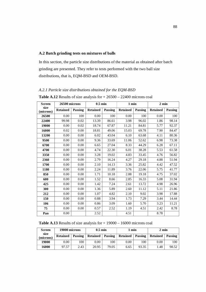
88

A.2 Batch grinding tests on mixtures of balls

In this section, the particle size distributions of the material as obtained after batch

grinding are presented. They refer to tests performed with the two ball size

distributions, that is, EQM-BSD and OEM-BSD.

A.2.1 Particle size distributions obtained for the EQM-BSD


Screen size

(microns)



26500 0.00

100 0.00 100 0.00 100 0.00 100 22400 99.98 0.02 13.39 86.61 3.98 96.02 1.86 98.14 19000 0.00 0.02 18.74 67.87 11.21 84.81 5.77 92.37 16000 0.02 0.00 18.81 49.06 15.03 69.78 7.90 84.47 13200 0.00 0.00 6.02 43.04 6.10 63.68 4.11 80.36 9500 0.00 0.00 9.36 33.69 11.06 52.62 6.98 73.38 6700 0.00 0.00 6.65 27.04 8.33 44.29 6.28 67.11 4700 0.00 0.00 4.74 22.30 6.01 38.28 5.53 61.58 3350 0.00 0.00 3.28 19.02 4.83 33.45 4.76 56.82 2360 0.00 0.00 2.79 16.24 4.27 29.18 4.88 51.94 1700 0.00 0.00 2.10 14.13 3.36 25.82 4.42 47.52 1180 0.00 0.00 2.24 11.89 3.76 22.06 5.75 41.77 850 0.00 0.00 1.71 10.18 2.88 19.18 4.75 37.02 600 0.00 0.00 1.52 8.66 2.85 16.33 5.08 31.94 425 0.00 0.00 1.42 7.24 2.61 13.72 4.98 26.96 300 0.00 0.00 1.36 5.89 2.60 11.12 5.11 21.86 212 0.00 0.00 1.07 4.82 2.10 9.02 3.98 17.88 150 0.00 0.00 0.88 3.94 1.73 7.29 3.44 14.44 106 0.00 0.00 0.86 3.09 1.60 5.70 3.23 11.21 75 0.00 0.00 0.57 2.52 1.19 4.51 2.42 8.78

Pan 0.00 2.52 4.51 8.78 Table A.13 Results of size analysis for + 19000 – 16000 microns coal

Screen size

(microns)



19000 0.00 100 0.00 100 0.00 100 0.00 100 16000 97.57 2.43 20.95 79.05 6.65 93.35 1.48 98.52

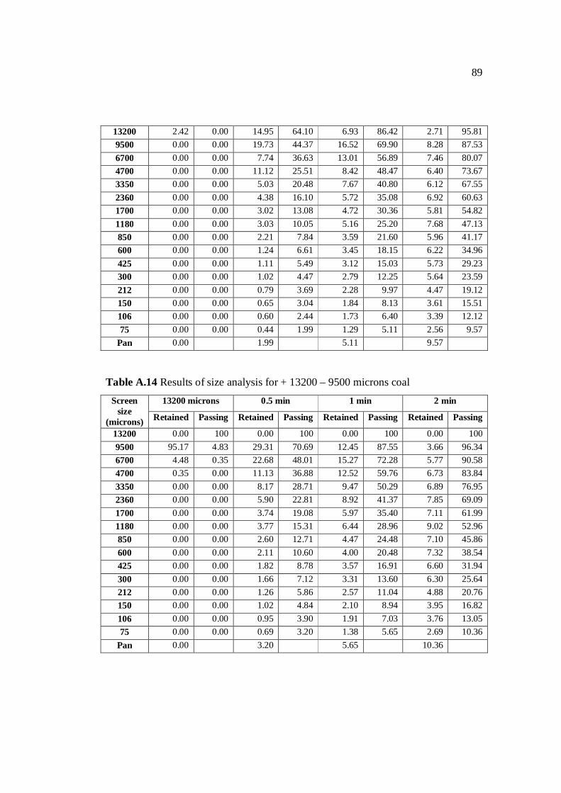
89

13200 2.42 0.00 14.95 64.10 6.93 86.42 2.71 95.81 9500 0.00 0.00 19.73 44.37 16.52 69.90 8.28 87.53 6700 0.00 0.00 7.74 36.63 13.01 56.89 7.46 80.07 4700 0.00 0.00 11.12 25.51 8.42 48.47 6.40 73.67 3350 0.00 0.00 5.03 20.48 7.67 40.80 6.12 67.55 2360 0.00 0.00 4.38 16.10 5.72 35.08 6.92 60.63 1700 0.00 0.00 3.02 13.08 4.72 30.36 5.81 54.82 1180 0.00 0.00 3.03 10.05 5.16 25.20 7.68 47.13 850 0.00 0.00 2.21 7.84 3.59 21.60 5.96 41.17 600 0.00 0.00 1.24 6.61 3.45 18.15 6.22 34.96 425 0.00 0.00 1.11 5.49 3.12 15.03 5.73 29.23 300 0.00 0.00 1.02 4.47 2.79 12.25 5.64 23.59 212 0.00 0.00 0.79 3.69 2.28 9.97 4.47 19.12 150 0.00 0.00 0.65 3.04 1.84 8.13 3.61 15.51 106 0.00 0.00 0.60 2.44 1.73 6.40 3.39 12.12 75 0.00 0.00 0.44 1.99 1.29 5.11 2.56 9.57


Screen size

(microns)



13200 0.00 100 0.00 100 0.00 100 0.00 100 9500 95.17 4.83 29.31 70.69 12.45 87.55 3.66 96.34 6700 4.48 0.35 22.68 48.01 15.27 72.28 5.77 90.58 4700 0.35 0.00 11.13 36.88 12.52 59.76 6.73 83.84 3350 0.00 0.00 8.17 28.71 9.47 50.29 6.89 76.95 2360 0.00 0.00 5.90 22.81 8.92 41.37 7.85 69.09 1700 0.00 0.00 3.74 19.08 5.97 35.40 7.11 61.99 1180 0.00 0.00 3.77 15.31 6.44 28.96 9.02 52.96 850 0.00 0.00 2.60 12.71 4.47 24.48 7.10 45.86 600 0.00 0.00 2.11 10.60 4.00 20.48 7.32 38.54 425 0.00 0.00 1.82 8.78 3.57 16.91 6.60 31.94 300 0.00 0.00 1.66 7.12 3.31 13.60 6.30 25.64 212 0.00 0.00 1.26 5.86 2.57 11.04 4.88 20.76 150 0.00 0.00 1.02 4.84 2.10 8.94 3.95 16.82 106 0.00 0.00 0.95 3.90 1.91 7.03 3.76 13.05 75 0.00 0.00 0.69 3.20 1.38 5.65 2.69 10.36

Pan 0.00 3.20 5.65 10.36

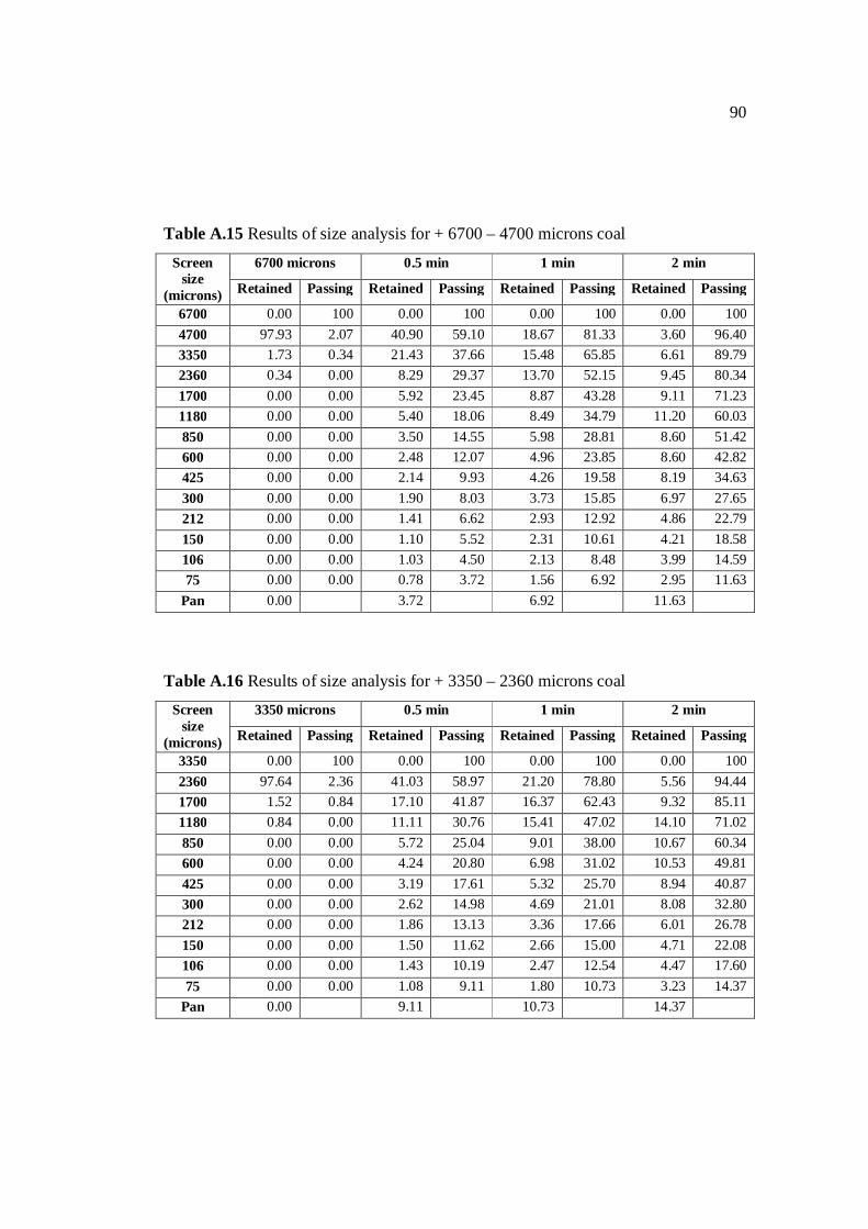
90


Screen size

(microns)



6700 0.00 100 0.00 100 0.00 100 0.00 100 4700 97.93 2.07 40.90 59.10 18.67 81.33 3.60 96.40 3350 1.73 0.34 21.43 37.66 15.48 65.85 6.61 89.79 2360 0.34 0.00 8.29 29.37 13.70 52.15 9.45 80.34 1700 0.00 0.00 5.92 23.45 8.87 43.28 9.11 71.23 1180 0.00 0.00 5.40 18.06 8.49 34.79 11.20 60.03 850 0.00 0.00 3.50 14.55 5.98 28.81 8.60 51.42 600 0.00 0.00 2.48 12.07 4.96 23.85 8.60 42.82 425 0.00 0.00 2.14 9.93 4.26 19.58 8.19 34.63 300 0.00 0.00 1.90 8.03 3.73 15.85 6.97 27.65 212 0.00 0.00 1.41 6.62 2.93 12.92 4.86 22.79 150 0.00 0.00 1.10 5.52 2.31 10.61 4.21 18.58 106 0.00 0.00 1.03 4.50 2.13 8.48 3.99 14.59 75 0.00 0.00 0.78 3.72 1.56 6.92 2.95 11.63


Screen size

(microns)



3350 0.00 100 0.00 100 0.00 100 0.00 100 2360 97.64 2.36 41.03 58.97 21.20 78.80 5.56 94.44 1700 1.52 0.84 17.10 41.87 16.37 62.43 9.32 85.11 1180 0.84 0.00 11.11 30.76 15.41 47.02 14.10 71.02 850 0.00 0.00 5.72 25.04 9.01 38.00 10.67 60.34 600 0.00 0.00 4.24 20.80 6.98 31.02 10.53 49.81 425 0.00 0.00 3.19 17.61 5.32 25.70 8.94 40.87 300 0.00 0.00 2.62 14.98 4.69 21.01 8.08 32.80 212 0.00 0.00 1.86 13.13 3.36 17.66 6.01 26.78 150 0.00 0.00 1.50 11.62 2.66 15.00 4.71 22.08 106 0.00 0.00 1.43 10.19 2.47 12.54 4.47 17.60 75 0.00 0.00 1.08 9.11 1.80 10.73 3.23 14.37

Pan 0.00 9.11 10.73 14.37

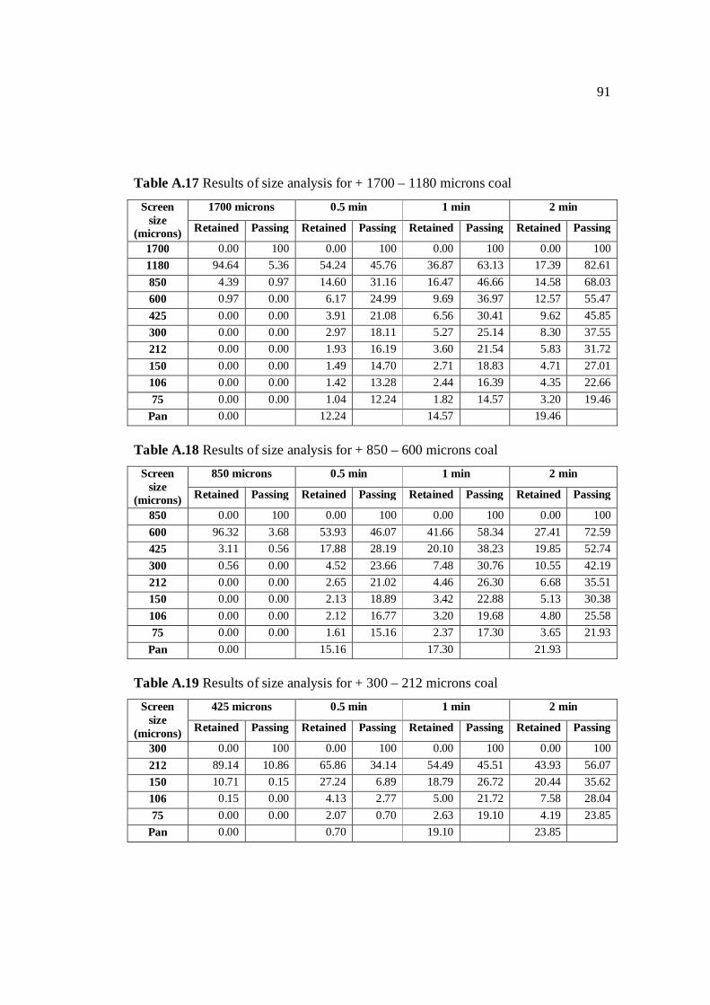
91


Screen size

(microns)



1700 0.00 100 0.00 100 0.00 100 0.00 100 1180 94.64 5.36 54.24 45.76 36.87 63.13 17.39 82.61 850 4.39 0.97 14.60 31.16 16.47 46.66 14.58 68.03 600 0.97 0.00 6.17 24.99 9.69 36.97 12.57 55.47 425 0.00 0.00 3.91 21.08 6.56 30.41 9.62 45.85 300 0.00 0.00 2.97 18.11 5.27 25.14 8.30 37.55 212 0.00 0.00 1.93 16.19 3.60 21.54 5.83 31.72 150 0.00 0.00 1.49 14.70 2.71 18.83 4.71 27.01 106 0.00 0.00 1.42 13.28 2.44 16.39 4.35 22.66 75 0.00 0.00 1.04 12.24 1.82 14.57 3.20 19.46


Screen size

(microns)



850 0.00 100 0.00 100 0.00 100 0.00 100 600 96.32 3.68 53.93 46.07 41.66 58.34 27.41 72.59 425 3.11 0.56 17.88 28.19 20.10 38.23 19.85 52.74 300 0.56 0.00 4.52 23.66 7.48 30.76 10.55 42.19 212 0.00 0.00 2.65 21.02 4.46

. 26.30 6.68 35.51

150 0.00 0.00 2.13 18.89 3.42 22.88 5.13 30.38 106 0.00 0.00 2.12 16.77 3.20 19.68 4.80 25.58 75 0.00 0.00 1.61 15.16 2.37 17.30 3.65 21.93


Screen size

(microns)



300 0.00 100 0.00 100 0.00 100 0.00 100 212 89.14 10.86 65.86 34.14 54.49 45.51 43.93 56.07 150 10.71 0.15 27.24 6.89 18.79 26.72 20.44 35.62 106 0.15 0.00 4.13 2.77 5.00 21.72 7.58 28.04 75 0.00 0.00 2.07 0.70 2.63 19.10 4.19 23.85

Pan 0.00 0.70 19.10 23.85

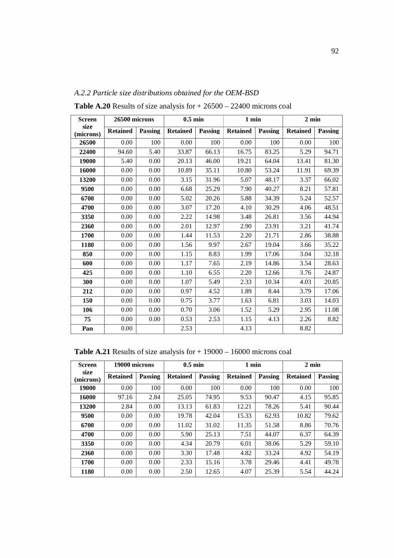
92

A.2.2 Particle size distributions obtained for the OEM-BSD


Screen size

(microns)



26500 0.00 100 0.00 100 0.00 100 0.00 100 22400 94.60 5.40 33.87 66.13 16.75 83.25 5.29 94.71 19000 5.40 0.00 20.13 46.00 19.21 64.04 13.41 81.30 16000 0.00 0.00 10.89 35.11 10.80 53.24 11.91 69.39 13200 0.00 0.00 3.15 31.96 5.07 48.17 3.37 66.02 9500 0.00 0.00 6.68 25.29 7.90 40.27 8.21 57.81 6700 0.00 0.00 5.02 20.26 5.88 34.39 5.24 52.57 4700 0.00 0.00 3.07 17.20 4.10 30.29 4.06 48.51 3350 0.00 0.00 2.22 14.98 3.48 26.81 3.56 44.94 2360 0.00 0.00 2.01 12.97 2.90 23.91 3.21 41.74 1700 0.00 0.00 1.44 11.53 2.20 21.71 2.86 38.88 1180 0.00 0.00 1.56 9.97 2.67 19.04 3.66 35.22 850 0.00 0.00 1.15 8.83 1.99 17.06 3.04 32.18 600 0.00 0.00 1.17 7.65 2.19 14.86 3.54 28.63 425 0.00 0.00 1.10 6.55 2.20 12.66 3.76 24.87 300 0.00 0.00 1.07 5.49 2.33 10.34 4.03 20.85 212 0.00 0.00 0.97 4.52 1.89 8.44 3.79 17.06 150 0.00 0.00 0.75 3.77 1.63 6.81 3.03 14.03 106 0.00 0.00 0.70 3.06 1.52 5.29 2.95 11.08 75 0.00 0.00 0.53 2.53 1.15 4.13 2.26 8.82

Pan 0.00 2.53 4.13 8.82


Screen size

(microns)



19000 0.00 100 0.00 100 0.00 100 0.00 100 16000 97.16 2.84 25.05 74.95 9.53 90.47 4.15 95.85 13200 2.84 0.00 13.13 61.83 12.21 78.26 5.41 90.44 9500 0.00 0.00 19.78 42.04 15.33 62.93 10.82 79.62 6700 0.00 0.00 11.02 31.02 11.35 51.58 8.86 70.76 4700 0.00 0.00 5.90 25.13 7.51 44.07 6.37 64.39 3350 0.00 0.00 4.34 20.79 6.01 38.06 5.29 59.10 2360 0.00 0.00 3.30 17.48 4.82 33.24 4.92 54.19 1700 0.00 0.00 2.33 15.16 3.78 29.46 4.41 49.78 1180 0.00 0.00 2.50 12.65 4.07 25.39 5.54 44.24

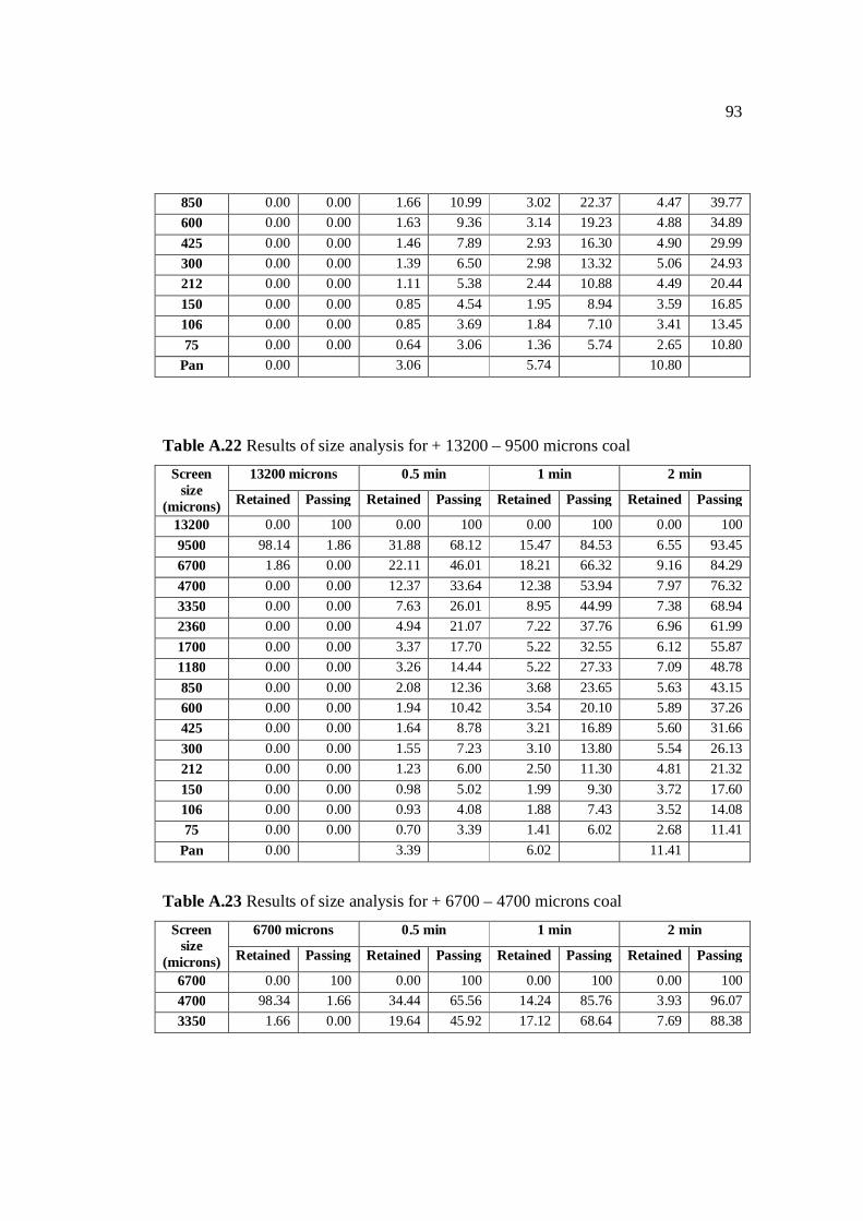
93

850 0.00 0.00 1.66 10.99 3.02 22.37 4.47 39.77 600 0.00 0.00 1.63 9.36 3.14 19.23 4.88 34.89 425 0.00 0.00 1.46 7.89 2.93 16.30 4.90 29.99 300 0.00 0.00 1.39 6.50 2.98 13.32 5.06 24.93 212 0.00 0.00 1.11 5.38 2.44 10.88 4.49 20.44 150 0.00 0.00 0.85 4.54 1.95 8.94 3.59 16.85 106 0.00 0.00 0.85 3.69 1.84 7.10 3.41 13.45 75 0.00 0.00 0.64 3.06 1.36 5.74 2.65 10.80

Pan 0.00 3.06 5.74 10.80


size (microns)



13200 0.00 100 0.00 100 0.00 100 0.00 100 9500 98.14 1.86 31.88 68.12 15.47 84.53 6.55 93.45 6700 1.86 0.00 22.11 46.01 18.21 66.32 9.16 84.29 4700 0.00 0.00 12.37 33.64 12.38 53.94 7.97 76.32 3350 0.00 0.00 7.63 26.01 8.95 44.99 7.38 68.94 2360 0.00 0.00 4.94 21.07 7.22 37.76 6.96 61.99 1700 0.00 0.00 3.37 17.70 5.22 32.55 6.12 55.87 1180 0.00 0.00 3.26 14.44 5.22 27.33 7.09 48.78 850 0.00 0.00 2.08 12.36 3.68 23.65 5.63 43.15 600 0.00 0.00 1.94 10.42 3.54 20.10 5.89 37.26 425 0.00 0.00 1.64 8.78 3.21 16.89 5.60 31.66 300 0.00 0.00 1.55 7.23 3.10 13.80 5.54 26.13 212 0.00 0.00 1.23 6.00 2.50 11.30 4.81 21.32 150 0.00 0.00 0.98 5.02 1.99 9.30 3.72 17.60 106 0.00 0.00 0.93 4.08 1.88 7.43 3.52 14.08 75 0.00 0.00 0.70 3.39 1.41 6.02 2.68 11.41

Pan 0.00 3.39 6.02 11.41


Screen size

(microns)



6700 0.00 100 0.00 100 0.00 100 0.00 100 4700 98.34 1.66 34.44 65.56 14.24 85.76 3.93 96.07 3350 1.66 0.00 19.64 45.92 17.12 68.64 7.69 88.38

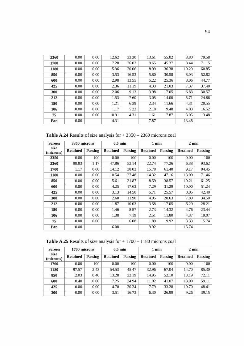
94

2360 0.00 0.00 12.62 33.30 13.61 55.02 8.80 79.58 1700 0.00 0.00 7.28 26.02 9.65 45.37 8.44 71.15 1180 0.00 0.00 5.96 20.06 8.99 36.38 10.29 60.85 850 0.00 0.00 3.53 16.53 5.80 30.58 8.03 52.82 600 0.00 0.00 2.98 13.55 5.22 25.36 8.06 44.77 425 0.00 0.00 2.36 11.19 4.33 21.03 7.37 37.40 300 0.00 0.00 2.06 9.13 3.98 17.05 6.83 30.57 212 0.00 0.00 1.53 7.60 3.05 14.00 5.71 24.86 150 0.00 0.00 1.21 6.39 2.34 11.66 4.31 20.55 106 0.00 0.00 1.17 5.22 2.18 9.48 4.03 16.52 75 0.00 0.00 0.91 4.31 1.61 7.87 3.05 13.48

Pan 0.00 4.31 7.87 13.48


Screen size

(microns)



3350 0.00 100 0.00 100 0.00 100 0.00 100 2360 98.83 1.17 47.86 52.14 22.74 77.26 6.38 93.62 1700 1.17 0.00 14.12 38.02 15.78 61.48 9.17 84.45 1180 0.00 0.00 10.54 27.48 14.32 47.16 13.00 71.46 850 0.00 0.00 5.61 21.87 8.59 38.57 10.21 61.25 600 0.00 0.00 4.25 17.63 7.29 31.29 10.00 51.24 425 0.00 0.00 3.13 14.50 5.71 25.57 8.85 42.40 300 0.00 0.00 2.60 11.90 4.95 20.63 7.89 34.50 212 0.00 0.00 1.87 10.03 3.58 17.05 6.29 28.21 150 0.00 0.00 1.46 8.57 2.73 14.32 4.76 23.44 106 0.00 0.00 1.38 7.19 2.51 11.80 4.37 19.07 75 0.00 0.00 1.11 6.08 1.89 9.92 3.33 15.74

Pan 0.00 6.08 9.92 15.74


size (microns)



1700 0.00 100 0.00 100 0.00 100 0.00 100 1180 97.57 2.43 54.53 45.47 32.96 67.04 14.70 85.30 850 2.03 0.40 13.28 32.19 14.95 52.10 13.19 72.11 600 0.40 0.00 7.25 24.94 11.02 41.07 13.00 59.11 425 0.00 0.00 4.70 20.24 7.79 33.28 10.70 48.41 300 0.00 0.00 3.51 16.73 6.30 26.99 9.26 39.15

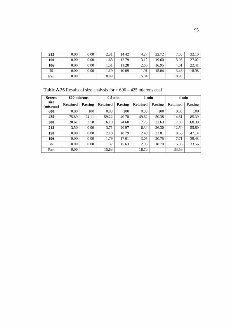
95

212 0.00 0.00 2.31 14.42 4.27 22.72 7.05 32.10 150 0.00 0.00 1.63 12.79 3.12 19.60 5.08 27.02 106 0.00 0.00 1.51 11.28 2.66 16.95 4.61 22.41 75 0.00 0.00 1.19 10.09 1.91 15.04 3.43 18.98

Pan 0.00 10.09 15.04 18.98


Screen size

(microns)



600 0.00 100 0.00 100 0.00 100 0.00 100 425 75.89 24.11 59.22 40.78 49.62 50.38 14.61 85.39 300 20.61 3.50 16.10 24.68 17.75 32.63 17.08 68.30 212 3.50 0.00 3.71 20.97 6.34 26.30 12.50 55.80 150 0.00 0.00 2.18 18.79 2.49 23.81 8.66 47.14 106 0.00 0.00 1.79 17.01 3.05 20.75 7.71 39.43 75 0.00 0.00 1.37 15.63 2.06 18.70 5.86 33.56

Pan 0.00 15.63 18.70 33.56

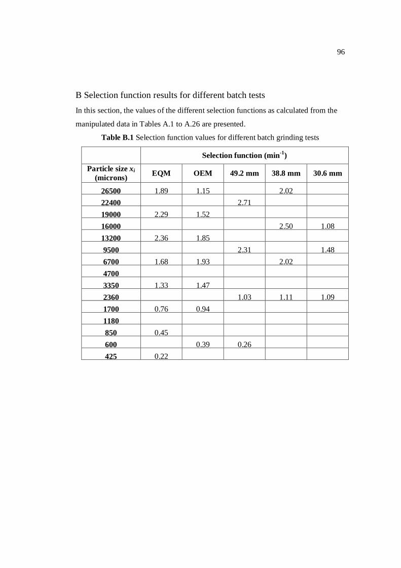
96

B Selection function results for different batch tests In this section, the values of the different selection functions as calculated from the

manipulated data in Tables A.1 to A.26 are presented.

Table B.1 Selection function values for different batch grinding tests

Selection function (min-1)

Particle size xi (microns) EQM OEM 49.2 mm 38.8 mm 30.6 mm

26500 1.89 1.15 2.02 22400 2.71 19000 2.29 1.52 16000 2.50 1.08 13200 2.36 1.85 9500 2.31 1.48 6700 1.68 1.93 2.02 4700 3350 1.33 1.47 2360 1.03 1.11 1.09 1700 0.76 0.94 1180 850 0.45 600 0.39 0.26 425 0.22

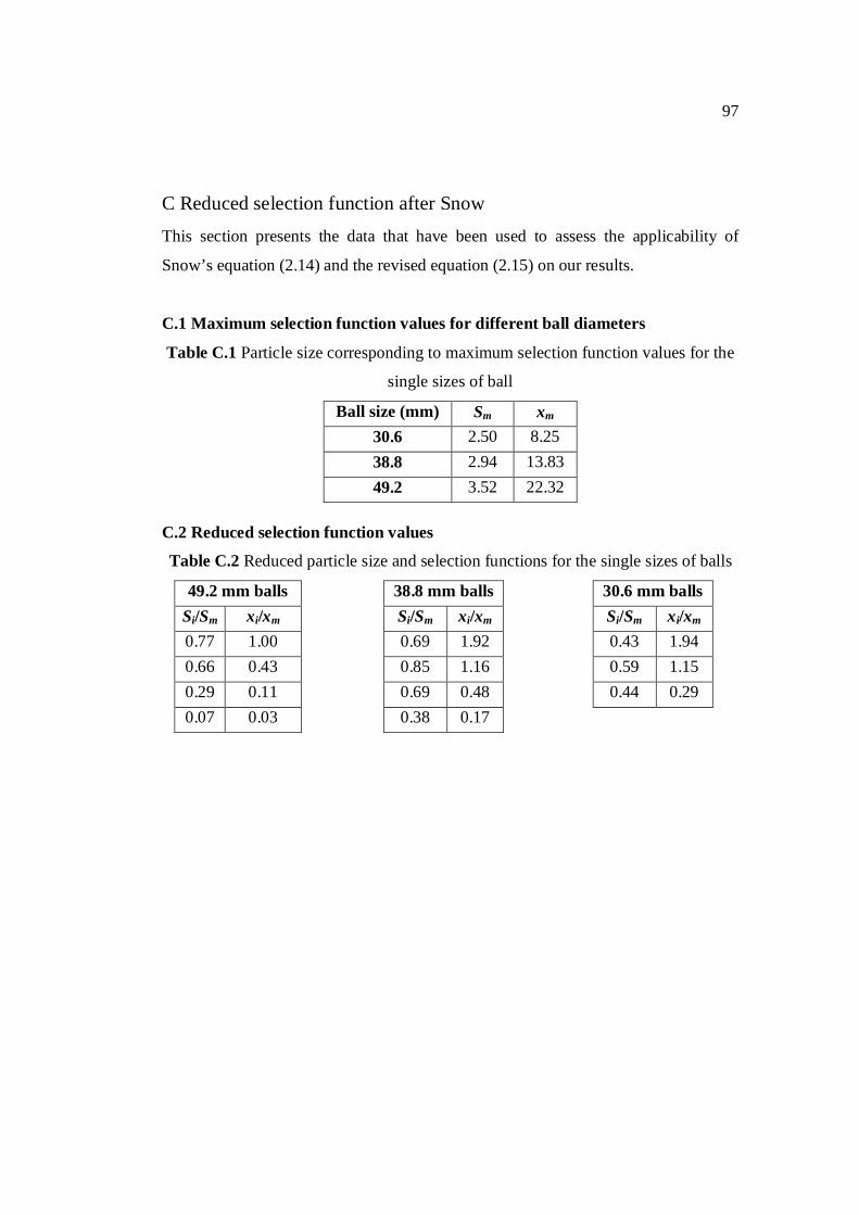
97

C Reduced selection function after Snow This section presents the data that have been used to assess the applicability of

Snow’s equation (2.14) and the revised equation (2.15) on our results.

C.1 Maximum selection function values for different ball diameters

Table C.1 Particle size corresponding to maximum selection function values for the

single sizes of ball

Ball size (mm) Sm xm 30.6 2.50 8.25 38.8 2.94 13.83 49.2 3.52 22.32

C.2 Reduced selection function values

Table C.2 Reduced particle size and selection functions for the single sizes of balls

49.2 mm balls Si/Sm xi/xm 0.77 1.00 0.66 0.43 0.29 0.11 0.07 0.03

38.8 mm balls Si/Sm xi/xm 0.69 1.92 0.85 1.16 0.69 0.48 0.38 0.17

30.6 mm balls Si/Sm xi/xm 0.43 1.94 0.59 1.15 0.44 0.29

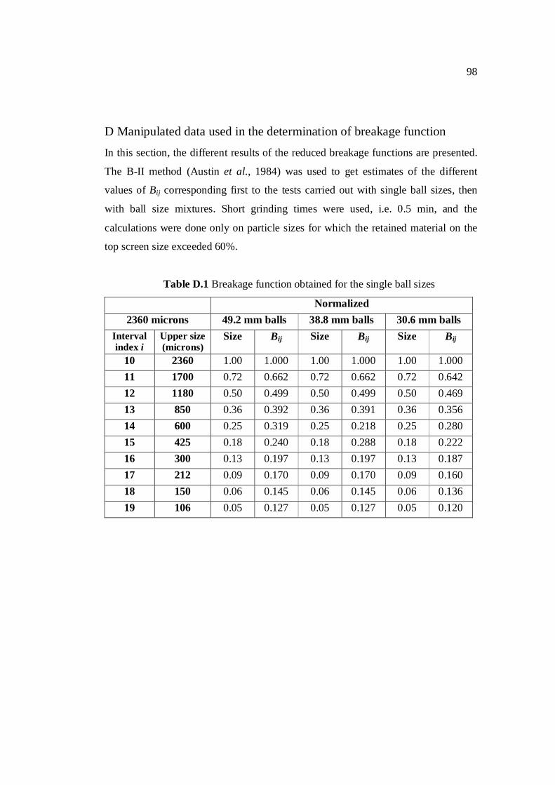
98

D Manipulated data used in the determination of breakage function In this section, the different results of the reduced breakage functions are presented.

The B-II method (Austin et al., 1984) was used to get estimates of the different

values of Bij corresponding first to the tests carried out with single ball sizes, then

with ball size mixtures. Short grinding times were used, i.e. 0.5 min, and the

calculations were done only on particle sizes for which the retained material on the

top screen size exceeded 60%.

Table D.1 Breakage function obtained for the single ball sizes

Normalized 2360 microns 49.2 mm balls 38.8 mm balls 30.6 mm balls

Interval index i

Upper size (microns)

Size Bij Size Bij Size Bij

10 2360 1.00 1.000 1.00 1.000 1.00 1.000 11 1700 0.72 0.662 0.72 0.662 0.72 0.642 12 1180 0.50 0.499 0.50 0.499 0.50 0.469 13 850 0.36 0.392 0.36 0.391 0.36 0.356 14 600 0.25 0.319 0.25 0.218 0.25 0.280 15 425 0.18 0.240 0.18 0.288 0.18 0.222 16 300 0.13 0.197 0.13 0.197 0.13 0.187 17 212 0.09 0.170 0.09 0.170 0.09 0.160 18 150 0.06 0.145 0.06 0.145 0.06 0.136 19 106 0.05 0.127 0.05 0.127 0.05 0.120

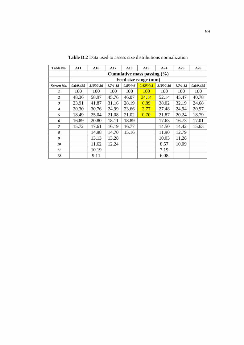
99

Table D.2 Data used to assess size distributions normalization

Table No. A11 A16 A17 A18 A19 A24 A25 A26 Cumulative mass passing (%) Feed size range (mm)

Screen No. 0.6/0.425 3.35/2.36 1.7/1.18 0.85/0.6 0.425/0.3 3.35/2.36 1.7/1.18 0.6/0.425 1 100 100 100 100 100 100 100 100 2 48.36 58.97 45.76 46.07 34.14 52.14 45.47 40.78 3 23.91 41.87 31.16 28.19 6.89 38.02 32.19 24.68 4 20.30 30.76 24.99 23.66 2.77 27.48 24.94 20.97 5 18.49 25.04 21.08 21.02 0.70 21.87 20.24 18.79 6 16.89 20.80 18.11 18.89 17.63 16.73 17.01 7 15.72 17.61 16.19 16.77 14.50 14.42 15.63 8 14.98 14.70 15.16 11.90 12.79 9 13.13 13.28 10.03 11.28 10 11.62 12.24 8.57 10.09 11 10.19 7.19 12 9.11 6.08

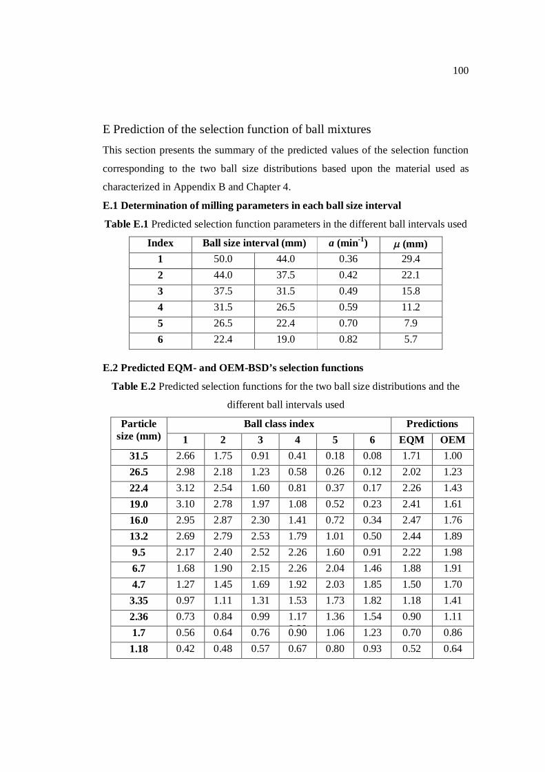
100

E Prediction of the selection function of ball mixtures This section presents the summary of the predicted values of the selection function

corresponding to the two ball size distributions based upon the material used as

characterized in Appendix B and Chapter 4.

E.1 Determination of milling parameters in each ball size interval

Table E.1 Predicted selection function parameters in the different ball intervals used

Index Ball size interval (mm) a (min-1) (mm) 1 50.0 44.0 0.36 29.4 2 44.0 37.5 0.42 22.1 3 37.5 31.5 0.49 15.8 4 31.5 26.5 0.59 11.2 5 26.5 22.4 0.70 7.9 6 22.4 19.0 0.82 5.7

E.2 Predicted EQM- and OEM-BSD’s selection functions

Table E.2 Predicted selection functions for the two ball size distributions and the

different ball intervals used

Particle size (mm)

Ball class index Predictions 1 2 3 4 5 6 EQM OEM

31.5 2.66 1.75 0.91 0.41 0.18 0.08 1.71 1.00 26.5 2.98 2.18 1.23 0.58 0.26 0.12 2.02 1.23 22.4 3.12 2.54 1.60 0.81 0.37 0.17 2.26 1.43 19.0 3.10 2.78 1.97 1.08 0.52 0.23 2.41 1.61 16.0 2.95 2.87 2.30 1.41 0.72 0.34 2.47 1.76 13.2 2.69 2.79 2.53 1.79 1.01 0.50 2.44 1.89 9.5 2.17 2.40 2.52 2.26 1.60 0.91 2.22 1.98 6.7 1.68 1.90 2.15 2.26 2.04 1.46 1.88 1.91 4.7 1.27 1.45 1.69 1.92 2.03 1.85 1.50 1.70 3.35 0.97 1.11 1.31 1.53 1.73 1.82 1.18 1.41 2.36 0.73 0.84 0.99 1.17

0.90 1.36 1.54 0.90 1.11

1.7 0.56 0.64 0.76 0.90 1.06 1.23 0.70 0.86 1.18 0.42 0.48 0.57 0.67 0.80 0.93 0.52 0.64

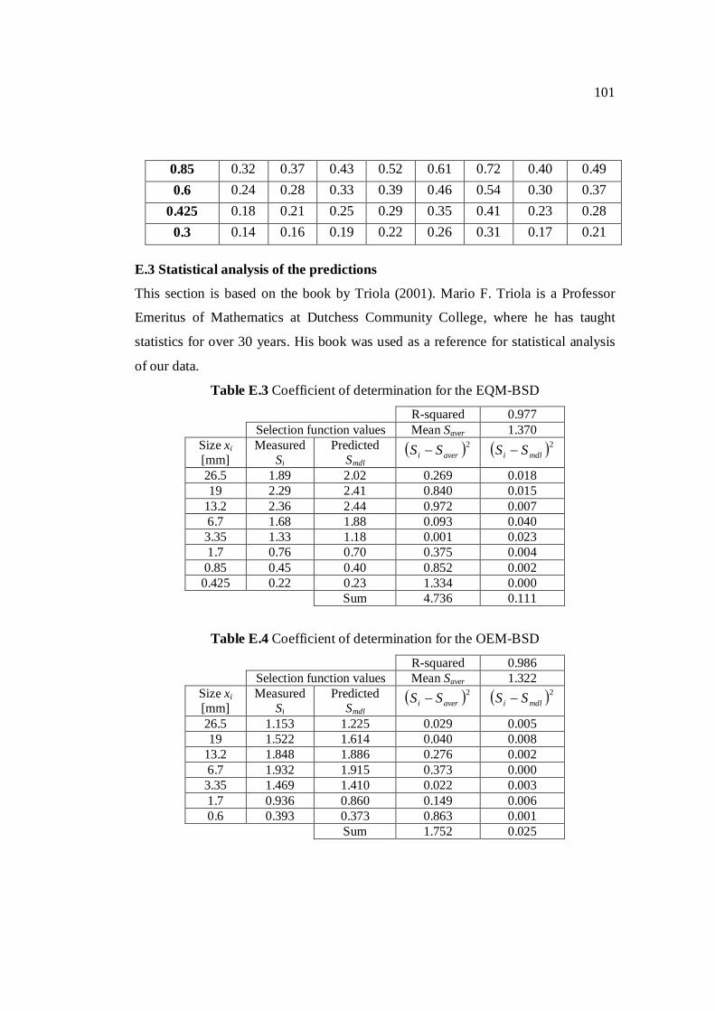
101

0.85 0.32 0.37 0.43 0.52 0.61 0.72 0.40 0.49 0.6 0.24 0.28 0.33 0.39 0.46 0.54 0.30 0.37

0.425 0.18 0.21 0.25 0.29 0.35 0.41 0.23 0.28 0.3 0.14 0.16 0.19 0.22 0.26 0.31 0.17 0.21

E.3 Statistical analysis of the predictions

This section is based on the book by Triola (2001). Mario F. Triola is a Professor

Emeritus of Mathematics at Dutchess Community College, where he has taught

statistics for over 30 years. His book was used as a reference for statistical analysis

of our data.

Table E.3 Coefficient of determination for the EQM-BSD

R-squared 0.977 Selection function values Mean Saver 1.370

Size xi [mm]

Measured Si

Predicted Smdl

2averi SS 2

mdli SS

26.5 1.89 2.02 0.269 0.018 19 2.29 2.41 0.840 0.015

13.2 2.36 2.44 0.972 0.007 6.7 1.68 1.88 0.093 0.040 3.35 1.33 1.18 0.001 0.023 1.7 0.76 0.70 0.375 0.004 0.85 0.45 0.40 0.852 0.002 0.425 0.22 0.23 1.334 0.000

Sum 4.736 0.111

Table E.4 Coefficient of determination for the OEM-BSD

R-squared 0.986 Selection function values Mean Saver 1.322

Size xi [mm]

Measured Si

Predicted Smdl

2averi SS 2

mdli SS

26.5 1.153 1.225 0.029 0.005 19 1.522 1.614 0.040 0.008

13.2 1.848 1.886 0.276 0.002 6.7 1.932 1.915 0.373 0.000 3.35 1.469 1.410 0.022 0.003 1.7 0.936 0.860 0.149 0.006 0.6 0.393 0.373 0.863 0.001

Sum 1.752 0.025

effect of ball size distribution on milling parameters … · effect of ball size distribution on...

Documents