educational simulator for teaching of particle swarm optimization...
TRANSCRIPT
1 TELEKONTRAN, VOL. 1, NO. 1, JANUARI 2013
Educational Simulator for Teaching of Particle Swarm
Optimization in LabVIEW
Perangkat Lunak Edukatif Berbasis LabVIEW sebagai Alat Bantu
Pengajaran Particle Swarm Optimization
Muhammad Aria Universitas Komputer Indonesia
Jl. Dipati ukur No 112, Bandung
Email : [email protected]
Abstract This paper presents an educational software tool for aid the teaching of Particle Swarm Optimization (PSO)
fundamentals with friendly design interface. This software were developed in the platform of LabVIEW
(Laboratory Virtual Intrumentation Engineering Workbench). The software‟s best qualities are users can
select many different version of the PSO algorithm, a lot of the benchmarks test functions for optimization
and set the parameters that have an influence on the PSO performance. Through visualization of particle
distribution in the searching, the simulator is particularly effective in providing users with an intuitive feel
for the PSO algorithm.
Keyword : Benchmark Function, LabVIEW, Particle Swarm Optimization, PSO Algorithm
Abstrak Paper ini mempresentasikan perancangan perangkat lunak pendidikan sebagai alat bantu pengajaran
materi Particle Swarm Optimization dengan desain antarmuka yang mudah digunakan. Perangkat lunak ini
dibuat berbasis LabVIEW (Laboratory Virtual Intrumentation Engineering Workbench). Keunggulan dari
perangkat lunak ini adalah pengguna mendapat pilihan banyak versi yang berbeda dari algoritma PSO,
terdapat banyak fungsi yang bisa digunakan untuk menguji proses optimasi dan dapat memodifikasi
parameter-parameter yang akan mempengaruhi performansi dari PSO. Dengan adanya visualisasi dari
pergerakan particle, perangkat lunak ini akan efektif untuk memberikan pemahaman mengenai prinsip
algoritma PSO kepada pengguna.
Kata Kunci – Fungsi benchmark, LabVIEW, Particle Swarm Optimization, Algoritma PSO
I. INTRODUCTION
Optimization problems are widely encountered
in various fields in technology. Some problems
can be very complex due to the actual and
practical nature of the objective function or the
model constraints. With the fast development of
industrial applications, optimization algorithms
encounter more and more challenges.
Optimization algorithms can be classified into
classical optimization based on gradient of
objective functions (e.g. Steepest Descent,
Conjugate Gradient Algorithm and Newton
Algorithm) and heuristic optimization algorithms
(e.g. Genetic Algorithms (GA), Simulated
Annealing (SA) and Particle Swarm Optimization
(PSO)). For some optimization problems, there is
no explicit analytical formula, so the gradient
information cannot be gained. And for high
dimension of problem, the classical algorithms are
sometimes not satisfying. Hence, population-
bases heuristic optimization algorithms, which not
require the derivative information of objective
functions and return a set of solutions at each
iteration, are more convenient for solving these
kinds of problems.
In 1995, Kennedy and Eberhart suggested a
PSO based on the analogy of swarm of bird and
school of fish (J. Kennedy et al., 1995). In PSO,
each individual makes his decision using his own
experience together with other individuals
experiences. The individual particles are drawn
stochastically toward the present velocity of each
individual, their own previous best performance
and the best previous performance of their
neighbours.
2 TELEKONTRAN, VOL. 1, NO. 1, JANUARI 2013
This paper would introduce an educational
simulator for the PSO algorithm. The purpose of
this simulator is to provide the users with useable
tool for gaining an intuitive feel for PSO
algorithm and mathematical optimization
problems. To aid the understanding PSO, the
simulator has been developed under the user-
friendly graphic user interface (GUI) environment
using LabVIEW. In this simulator, the users can
select many different version of the PSO
algorithm and set parameters related to the
performance of PSO and can observe the impact
of the parameters to the solution quality. This
simulator also displayed the movements of each
particle and convergence process of a group. This
educational simulator is used in Artificial
Intelligent and Intelligent Control course of
Electrical Engineering and Computer Engineering
Graduate Program at Universitas Komputer
Indonesia.
Some researchers have integrated PSO into
different kinds of toolboxes. Lee and Park
developed Educational Simulator for Particle
Swarm Optimization and Economic Dipatch
Applications based on MATLAB (W. N. Lee et
al., 2011). Coelho and Sierakowski developed A
Software tool for teaching particle swarm
optimization fundamental based on MATLAB
(L.d.S. Coelhu et al., 2008). Qi, Hu and Cournede
developed a particle swarm optimization in Scilab
(R.Qi et al., 2009). However, most of them are
implemented in MATLAB or Scilab. As far as the
author concerns, there is no work on development
of educational simulator for particle swarm
optimization based on LabVIEW. This toolbox
can be widely used, not simply as a „black box‟,
but also as a basis to understand the principles of
optimization algorithms by making it possible for
user to easily read, change or tune algorithms and
algorithm parameters.
The paper is arranged as follows. Overview of
particle swarm optimization are descibed in
Section II. In Section III The features of
educational PSO simulator are introduced.
Mathematical optimization problems is presented
in Section IV. Its performance is analyzed in
Section V. Finally, the conclusion is given in
Section VI.
II. PARTICLE SWARM
OPTIMIZATION
PSO is a kind of heuristic optimization
algorithms. It is motivated from simulating certain
simplified animal social behaviors such as bird
flocking. It is an iterative and population-based
method. The particles are descibed by their two
instinct properties: position and velocity. The
position of each particle represents a point in the
parameter space, which a possible solution of the
optimization problem, and the velocity is used to
change the position.
A. The Original Particle Swarm
Optimization Algorithm
In order to optimize an unconstrained 𝑑-
dimensional objective function 𝑓 ∶ ℝ𝑑 → ℝ, the
original PSO algorithm [J. Kennedy, et al. (1995)]
is initialized with a population of complete
solutions (called particles) 𝑝1 , … , 𝑝𝑘 = 𝒫 are
randomly initialized in the solution space. The
objective function determines the quality of a
particle‟s position, that is, the quality of the
solution it represents.
Each particle 𝑝𝑖 at time step 𝑡 has a position
vector 𝑥𝑖 𝑡 and a associated velocitiy vector 𝑣𝑖
𝑡.
Every particle “remembers” the position in which
it has received the best evaluation of the objective
function. This memory is represents by vector
𝑝𝑏𝑒 𝑠𝑡𝑖 . This vector is updated every time particle
𝑝𝑖 finds a better position. At the swarm level, the
vector 𝑔𝑏𝑒 𝑠𝑡 stores the best position any particle
has ever visited.
The algorithm iterates updating particles
velocity and position until a stopping criterion is
met, usually a maximum number of iterations or a
sufficiently good solution. The update rules are :
𝑣𝑖 𝑡+1
= 𝑣𝑖 𝑡
+ 𝜑1 ∙ 𝑈 1 0,1 ∗ 𝑝𝑏𝑒 𝑠𝑡𝑖 −
𝑥𝑖 𝑡 + 𝜑2 ∙ 𝑈 2 0,1 ∗ 𝑔𝑏𝑒 𝑠𝑡 −
𝑥𝑖 𝑡
(1)
𝑥𝑖 𝑡+1
= 𝑥𝑖 𝑡
+ 𝑣𝑖 𝑡+1
(2)
Where 𝜑1 and 𝜑2 are two constant called the
cognitive and social acceleration coefficients
repectively, 𝑈 1 0,1 and 𝑈 2 0,1 are two d-
dimensional uniformly distributed random vector
(generated every iteration) in which each
component goes from zero to one, and ∗ is an
element-by-element vector multiplication

3 TELEKONTRAN, VOL. 1, NO. 1, JANUARI 2013
operator. The values of 𝜑1 and 𝜑2 are parameters
of the algorithm.
In the original PSO algorithm a particle has
two attractors: its own previous best position and
the swarm‟s global best position. Previous
experience with population-based optimization
algorithms dictated that a strong bias towards the
best solution so far may lead to premature
convergence. Therefore, the local version of the
PSO algorithm was devised.
The variants we include in this study selected
either because they are among the most
commonly used in the field or because they look
promising.
B. Local Particle Swarm Optimizer
An early variant of the original PSO algorithm
was proposed by Eberhart and Kennedy [R.
Eberhart, et al. (1995)] in which a particle does
not accelerate towards the swarm‟s global best
solution. Instead, it accelerates towards the best
solution found within its local topological
neighborhood. A particle 𝑝𝑖 has a topological
neighborhood 𝒩𝑖 ⊆ 𝒫 (𝒫 = 𝑝1 , … , 𝑝𝑘 is the set
of particles in the swarm) of particles.
In the local PSO algorithm, Equation (2)
becomes
𝑣𝑖 𝑡+1
= 𝑣𝑖 𝑡
+ 𝜑1 ∙ 𝑈 1 0,1 ∗ 𝑝𝑏𝑒 𝑠𝑡𝑖 −
𝑥𝑖 𝑡 + 𝜑2 ∙ 𝑈 2 0,1 ∗ 𝑙𝑏𝑒 𝑠𝑡𝑖
−
𝑥𝑖 𝑡
(3)
Where vector 𝑙𝑏𝑒 𝑠𝑡𝑖 stores the best position in the
neighborhood has ever visited. Mohais et al. [A.
Mohais, et.al. (2005)] reported that random
topologies have the same or even better
performance than nonrandom topologies.
C. Canonical Particle Swarm Optimizer
Clerc and Kennedy [M. Clerc, et al. (2002)]
introduced a constriction factor into the velocity
update rule of the original PSO algorithm. The
purpose of this factor is to avoid particles
velocities to increase towards infinity and to
control the convergence properties of the
particles.
This constriction factor is added to Equation
(3) giving
𝑣𝑖 𝑡+1
= 𝒳 ∙ 𝑣𝑖 𝑡
+ 𝜑1 ∙ 𝑈 1 0,1 ∗ 𝑝𝑏𝑒 𝑠𝑡𝑖
− 𝑥𝑖 𝑡 + 𝜑2 ∙ 𝑈 2 0,1 ∗ 𝑙𝑏𝑒 𝑠𝑡𝑖
−
𝑥𝑖 𝑡
(4)
with
𝒳 =2 ∙ 𝑘
2 − 𝜑 − 𝜑2 − 4𝜑
(5)
where 𝑘 ∈ 0,1 , 𝜑 = 𝜑1 + 𝜑2 and 𝜑 > 4.
Usually, 𝑘 is set to 1 and both 𝜑1 and 𝜑2 are set
to 2.05, giving as a results 𝒳 equal to 0.729.
D. Time-Varying Decreasing Inertia
Weight Particle Swarm Optimizer
Shi and Eberhart [Y. Shi, et al. (1999)]
introduced the idea of a control factor called
inertia weight to control the diversification-
intensification behavior of the original PSO. The
velocity update rule was modified as follows
𝑣𝑖 𝑡+1
= 𝑤 𝑡 ∙ 𝑣𝑖 𝑡
+ 𝜑1 ∙ 𝑈 1 0,1 ∗
𝑝𝑏𝑒 𝑠𝑡𝑖 − 𝑥𝑖 𝑡 + 𝜑2 ∙ 𝑈 2 0,1
∗ 𝑙𝑏𝑒 𝑠𝑡𝑖 − 𝑥𝑖 𝑡
(6)
where 𝑤 𝑡 is the inertia weight which is usually
a time-dependent function. 𝜑1 and 𝜑2 are set to 2.
Since we want the algorithm to explore the
search space during the first iterations and focus
on the promising regions afterwards, 𝑤 𝑡 should
be a time-decreasing function of time.
The function used to schedule the inertia
weight is defined as
𝑤 𝑡 = 𝑤𝑚𝑎𝑥 − 𝑤𝑚𝑎𝑥 − 𝑤𝑚𝑖𝑛 ∙ 𝑡
𝑡𝑚𝑎𝑥 (7)
where 𝑡𝑚𝑎𝑥 marks the time at which 𝑤 𝑡 =𝑤𝑚𝑖𝑛 , 𝑤𝑚𝑎𝑥 and 𝑤𝑚𝑖𝑛 are the maximum and
minimum values the inertia weight can take. The
most widely used approach, is the one that uses a
decreasing inertia weight with a starting value of
0.9 and 0.4 as the final one.
4 TELEKONTRAN, VOL. 1, NO. 1, JANUARI 2013
E. Time-Varying Increasing Inertia
Weight Particle Swarm Optimizer
Zheng [Y.L. Zheng, et al. (2003)] studied the
effects of using a time-increasing inertia weight
function showing also that, in some cases, it
provides a faster convergence rate.
The function used to schedule the inertia weight
is defined as
𝑤 𝑡 = 𝑤𝑚𝑖𝑛 − 𝑤𝑚𝑖𝑛 − 𝑤𝑚𝑎𝑥 ∙ 𝑡
𝑡𝑚𝑎𝑥 (8)
Zheng et al., use increasing inertia weight with a
starting value of 0.4 and the final value 0.9.
F. Time-Varying Stochastic Inertia
Weight Particle Swarm Optimizer
Eberhart and Shi [R. Eberhart, et al. (2001)]
proposed another variant in which the inertia
weight is randomly selected according to a
uniform distribution in the range [0..5, 1.0]. This
range was inspired by Clerc and Kennedy‟s
constriction factor because the expected value of
the inertia weight in this case in 0.75 ≈ 0.729.
G. Fully Informed Particle Swarm
Optimizer
Mendes et al. [R. Mendes, et. Al. (2004)]
proposed the fully informed particle swarm, in
which a particle uses information provided by all
its neighbors in order to update its velocity.
The new velocity update equation becomes
𝑣𝑖 𝑡+1
= 𝒳 𝑣𝑖 𝑡
+ 𝜑𝑘 ∙ 𝒲 𝑝𝑏𝑒 𝑠𝑡𝑘
𝒫𝑘∈𝒩𝑖
∙
𝑈 𝑘 0,1 ∗ 𝑝𝑏𝑒 𝑠𝑡𝑘 − 𝑥𝑖 𝑡
(9)
where 𝒩𝑖 is the neighborhood of particle 𝑖, 𝒲 𝑝𝑏𝑒 𝑠𝑡𝑘 is a weighting function. The goal of
𝒲 𝑝𝑏𝑒 𝑠𝑡𝑘 is to provide information about the
quality of the attractor 𝑝𝑏𝑒 𝑠𝑡𝑖 . For example, the
normalized objective function value of the vector
𝑝𝑏𝑒 𝑠𝑡𝑖 could serve well.
H. Self Organizing Hierarchical Particle
Swarm Optimizer with Time-varying
Acceleration Coefficients
Proposed by Ratnaweera [A. Ratnaweera, et al.
(2004)], in HPSOTVAC, if any component of a
particle‟s velocity vector becomes zero, it is
reinitialized to a value proportional to the
maximum allowable velocity 𝑉𝑚𝑎𝑥 . To amplify
the local search behaviour of the swarm,
HPSOTVAC linearly adapts the value of the
acceleration coefficients 𝜑1 and 𝜑2. The cognitive
coefficient, 𝜑1, is decreased from 2.5 to 0.5 and
the social coefficient, 𝜑2, is increased from 0.5 to
2.5.
To avoid the problem of setting a proper
reinitialization velocity, HPSOTVAC linearly
decreases it from 𝑉𝑚𝑎𝑥 at the beginning of the run
to 0.1 ∙ 𝑉𝑚𝑎𝑥 at the end. As in the time-decreasing
inertia weight variant, a low reinitialization
velocity near the end of the run, allows particles
to move slowly near the best region they found.
I. Hierarchical Particle Swarm
Optimizer
In H-PSO, all particles are arranged in a
hierarchy that defines the neighborhood structure.
Each particle is neighbored to itslef and its parent
in the hierarchy. In this research we used reguler
tree like hierarchies. The hierarchy is defined by
the height , the branching degree 𝑑, the
maximum number of children of the inner nodes
and the total number of nodes 𝑚 of the
corresponding tree. We use only hierarchies in
which all inner nodes have the same number of
children, only the inner nodes on the deepest level
might have a smaller number of children.
The new position of the particles within the
hierarchy are determined as follows. For every
particle 𝑗 in a node of the tree, its own best
solution is compared to the best solution found by
the particles in the child nodes. If the best of these
particles is better, then child particles and parents
particles swap their place within the hierarchy.
For the update of the velocities in AH-PSO, a
particle is influenced by its own so far best
position and by the best position of the individual
that is directly above in the hierarchy.
Similar as in PSO, after the particles velocities
are updated and after the particles have moved in
H-PSO, the objective function is evaluated at the
new position. If the function value at this position
is better than the function value at the personal
best position, the personal best position is update.
J. Adaptive Hierarchical Particle Swarm
Optimizer

5 TELEKONTRAN, VOL. 1, NO. 1, JANUARI 2013
Proposed by Janson and Middendorf [S.
Janson, et al. (2005)], In the Adaptive H-PSO
(AH-PSO) , the branching degree is gradually
decreased during a run of the algorithm by 𝑘𝑎𝑑𝑎𝑝𝑡
degrees until a certain minimum degree 𝑑𝑚𝑖𝑛 is
reached. This process takes place every 𝑓𝑎𝑑𝑎𝑝𝑡
number of iterations
K. Estimation of Distribution Particle
Swarm Optimizer
Proposed by Iqbal, [M. Iqbal, et al.], the
EDPSO borrows some ideas from 𝐴𝐶𝑂ℝ. EDPSO
works as a canonical PSO but with some
modifications : after the execution of the velocity
update rule shown in Equation (4), EDPSO selects
one Gaussian function. Then, the selected
Gaussian function is evaluated to probabilistically
move the particle to its new position. If the
movement is successful, the algorithm continues
as usual, but if the movement is unsuccessful,
then the selected Gaussian function is sampled in
the same way as 𝐴𝐶𝑂ℝ.
III. EDUCATIONAL PSO
SIMULATOR
This educational PSO simulator can solve
maximization or minimization problems without
transforming the formulas of optimization
problems. It can show convergence curve in real-
time and particle distribution in the searching
space. This educational PSO simulator considers
different PSO algorithm. The variants of PSO
algorithm integrated into this educational PSO
simulator are listed in Table 2.
Table 2. Variants of PSO algorithm integrated
into simulator
Algorithm Reference
Original PSO J. Kennedy, et al.
(1995)
Local PSO R. Eberhart, et al.
(1995)
Canonical PSO M. Clerc, et al.
(2002)
Decreasing Inertia
Weight PSO Y. Shi, et al. (1999)
Increasing Inertia
Weight PSO
Y.L. Zheng, et al.
(2003)
Stochastic Inertia
Weight PSO
R. Eberhart, et al.
(2001)
Fully Informed PSO R. Mendes, et. Al.
(2004)
Self-Organizing
Hierarchical PSO with
Time-Varying
Acceleration
Coefficients
A. Ratnaweera, et
al. (2004)
Hierarchical PSO C.-C. Chen (2009)
Adaptive Hierarchical
PSO
S. Janson, et al.
(2005)
Estimation of
Ditribution PSO M. Iqbal, et al
The educational PSO simulator are arranged in
three layers : Functions Selection, 3D Function
Display dan Optimization Process. In the
Functions Selection Layers, the user can select the
mathematical function problem. Figure 1 show
the main view of the Educational PSO Simulator.
At least there are 100 function available which
user can select. Figure 2 show the Function
Selection Layers. In the left of the front panel is
the list of mathematical function available to
select.
Figure 1. Front Panel of Educational PSO
Simulator
Figure 2. Functions Selection Layers
Figure 3. 3D Function Display Layers
6 TELEKONTRAN, VOL. 1, NO. 1, JANUARI 2013
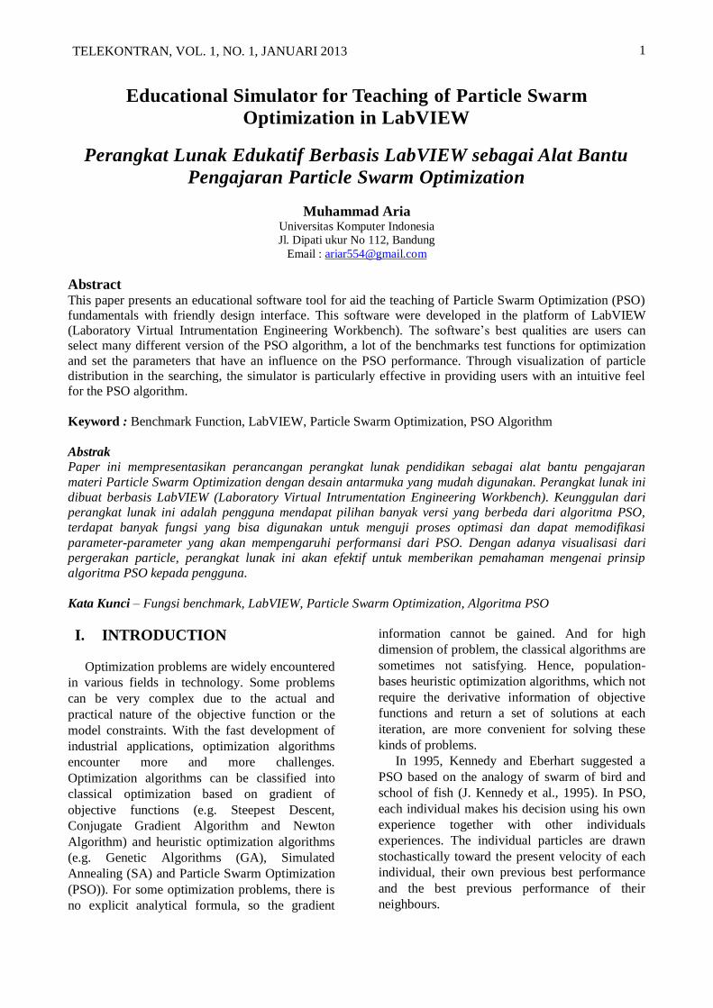
Figure 4. Optimization Process Layers
3D Function Display Layers is used to display
the function in 3D view. The user can rotate the
function to get better view of the problem. Figure
3 show the 3D Function Display Layers of the
Educational PSO Simulator.
The Optimization Process Layers is used to set
the PSO algorithm, to set parameters that have an
influence on the PSO performance and to
visualization process of each particle. Figure 4
show the Optimization Process Layers.
IV. MATHEMATICAL
OPTIMIZATION PROBLEMS
Several kinds of function benckmark problems
are chosen to demonstrate the performace of
simulator. For the case study, we choose 5
mathematical examples : (i) Sphere function, (ii)
Rosenbrock function, (iii) Ackley‟s function, (iv)
Rastrigin function, (v) Griewank function.
The function and the range of input variables
of Sphere Function are as follows :
min𝑥
𝑓 𝑥 = 𝑥𝑖2
𝑁
𝑖=1
−5.12 ≤ 𝑥𝑖 ≤ 5.12
(10)
The function and the range of input variables
of Schaffer Function are as follows :
min𝑥
𝑓 𝑥 = 0.5 +𝑎 𝑥
𝑏 𝑥
𝑎 𝑥 = 𝑠𝑖𝑛2 𝑥12 + 𝑥2
2 − 0.5
𝑏 𝑥 = 1 + 0.001 𝑥12 + 𝑥2
2 2
−100 ≤ 𝑥𝑖 ≤ 100
(11)
The function and the range of input variables
of Ackley‟s Function are as follows :
min𝑥
𝑓 𝑥 = 𝑎 𝑥 + 𝑏 𝑥 + 20 + 𝑒1
𝑎 𝑥 = −20 ∙ 𝑒𝑥𝑝 −0.2 1
𝑁 𝑥𝑖
2𝑁
𝑖=1
𝑏 𝑥 = −𝑒𝑥𝑝 1
𝑁 cos 2𝜋 ∙ 𝑥𝑖
𝑁
𝑖=1
−32.768 ≤ 𝑥𝑖 ≤ 32.768
(12)
The function and the range of input variables
of Rastrigin Function are as follows :
min𝑥
𝑓 𝑥 = 10𝑁 + 𝑥𝑖2 −
𝑁
𝑖=1
10 cos 2𝜋𝑥𝑖
−5.12 ≤ 𝑥𝑖 ≤ 5.12
(13)
The function and the range of input variables
of Shekel‟s Foxholes Function are as follows :
min𝑥
𝑓 𝑥 =1
0.002 + 𝑔 𝑥
𝑔 𝑥 = 1
𝑗 + 𝑥1 − 𝑎1𝑗 6
+ 𝑥2 − 𝑎2𝑗 6
25
𝑗 =1
𝑎𝑖𝑗 = −32 −16 0 … 32−32 −32 −32 … 32
−65.536 ≤ 𝑥𝑖 ≤ 65.536
(14)
V. EXAMPLES
In this section, Simulator is run in Windows 7
platform in the version of LabVIEW 7.
A. Visualization Process
The series picture in Figure 5 shows a run of
the Fully Informed Particle Swarm on the Sphere
Function. Specifically it shows the 0th, 20th, 40th,
60th, 80th and 100th iterations of the run. As the
particles continue in the run, they reach lower and
lower fitness values (signified by an inceased
amount of yellow dot) thus minimizing the
function. Figure 5 also displayed the convergence
process of a group.

7 TELEKONTRAN, VOL. 1, NO. 1, JANUARI 2013
(a) 0th iterations
(b) 20th iterations
(c) 40th iterations
(d) 60th iterations
(e) 80th iterations
(f) 100th iterations
Figure 5. A run of Simulator on the Sphere
FUnction
B. Parameter Settings
We decide to test the particle swarm
optimizers that we included in our study without
tuning their set of parameters specifically for each
test problem. All algorithms were run with the
same set of parameters over all test problems. The
specific parameter settings were those that are
normally used in the literature. Table 4 lists the
algorithms fixed parameter settings that we use in
our experiments.
The maximum number of evaluations to find a
solution was set to 100. We ran the algorithms
100 times on each problem. Maximum velocity
𝑉𝑚𝑎𝑥 is clamped to ±𝑋𝑚𝑎𝑥 where 𝑋𝑚𝑎𝑥 is the
maximum of the search range.
Table 4. Algorithm fixed parameter settings
Algorithm Settings
Original
PSO
Cognitive component 𝜑1 = 2.05
Social component 𝜑2 = 2.05
Local PSO
Cognitive component 𝜑1 = 2.05
Social component 𝜑2 = 2.05
Number of Neighborhood = 3

8 TELEKONTRAN, VOL. 1, NO. 1, JANUARI 2013
Canonical
PSO
Cognitive component 𝜑1 = 2.05
Social component 𝜑2 = 2.05
Constriction factor 𝒳 = 0.729
Number of Neighborhood = 3
Decreasing
Inertia
Weight
Cognitive component 𝜑1 = 2.05
Social component 𝜑2 = 2.05
Initial inertia weight = 0.9
Final inertia weight = 0.4
Number of Neighborhood = 3
Increasing
Inertia
Weight
Cognitive component 𝜑1 = 2.05
Social component 𝜑2 = 2.05
Final inertia weight = 0.9
Initial inertia weight = 0.4
Number of Neighborhood = 3
Stochastic
Inertia
Weight
Cognitive component 𝜑1 = 2.05
Social component 𝜑2 = 2.05
Minimum inertia weight = 0.4
Maximum inertia weight = 0.9
Number of Neighborhood = 3
Fully
Informed
PSO
Sum of the acc. coeff. 𝜑 = 4.1
Constriction factor 𝒳 = 0.729
Number of Neighborhood = 3
Self
Organizing
Hierarchical
PSO
Initial value of 𝜑1 = 2.5
Final value of 𝜑1 = 0.5
Initial value of 𝜑2 = 0.5
Final value of 𝜑2 = 0.5
Number of Neighborhood = 3
Hierarchical
PSO
Cognitive component 𝜑1 = 2
Social component 𝜑2 = 2
w = 0.9
r = 0.95
height of the tree (h) = 3
branching degree (d) = 4
Adaptive
Hierarchical
PSO
Cognitive component 𝜑1 = 2.05
Social component 𝜑2 = 2.05
Constriction factor 𝒳 = 0.729
Initial Branching factor = 20
d min = 2
f adapt/m = 10
k adapt = 3
Estimation
of
Distribution
PSO
Cognitive component 𝜑1 = 2.05
Social component 𝜑2 = 2.05
Constriction factor 𝒳 = 0.729
q = 0.1
epsilone = 0.85
C. Convergence Results
Two input variables (i.e., 2-dimensional space)
have been set in order to show the movement of
particles on contour. 30 independent trials are
conducted to observe the variation during the
evoltionary processes and compare the solution
quality and convergence characteristics.
To successfully implement the PSO, some
parameters must be assigned in advance. The
population size NP is set to 20. Since the
performance of PSO depends on its parameters
such as inertia weight or acceleration coefficients,
it is very important to determine the suitable
values of parameters.
Initial and final stages of the optimization
process for the Sphere function are shown if
Figure 6.
(a) Initial stage
(b) Final stage
Figure 6. Optimization process for the Sphere
Function
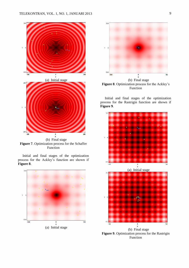
Initial and final stages of the optimization
process for the Schaffer function are shown if
Figure 7.
9 TELEKONTRAN, VOL. 1, NO. 1, JANUARI 2013
(a) Initial stage
(b) Final stage
Figure 7. Optimization process for the Schaffer
Function
Initial and final stages of the optimization
process for the Ackley‟s function are shown if
Figure 8.
(a) Initial stage
(b) Final stage
Figure 8. Optimization process for the Ackley‟s
Function
Initial and final stages of the optimization
process for the Rastrigin function are shown if
Figure 9.
(a) Initial stage
(b) Final stage
Figure 9. Optimization process for the Rastrigin
Function
10 TELEKONTRAN, VOL. 1, NO. 1, JANUARI 2013
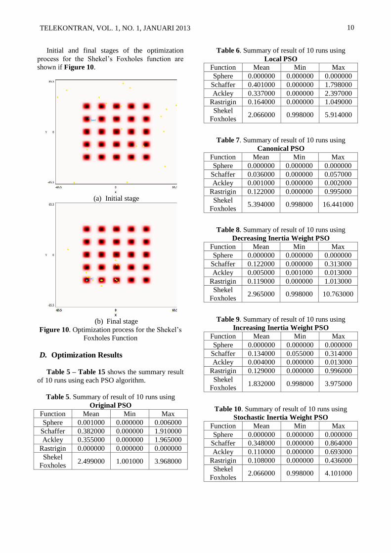
Initial and final stages of the optimization
process for the Shekel‟s Foxholes function are
shown if Figure 10.
(a) Initial stage
(b) Final stage
Figure 10. Optimization process for the Shekel‟s
Foxholes Function
D. Optimization Results
Table 5 – Table 15 shows the summary result
of 10 runs using each PSO algorithm.
Table 5. Summary of result of 10 runs using
Original PSO
Function Mean Min Max
Sphere 0.001000 0.000000 0.006000
Schaffer 0.382000 0.000000 1.910000
Ackley 0.355000 0.000000 1.965000
Rastrigin 0.000000 0.000000 0.000000
Shekel
Foxholes 2.499000 1.001000 3.968000
Table 6. Summary of result of 10 runs using
Local PSO
Function Mean Min Max
Sphere 0.000000 0.000000 0.000000
Schaffer 0.401000 0.000000 1.798000
Ackley 0.337000 0.000000 2.397000
Rastrigin 0.164000 0.000000 1.049000
Shekel
Foxholes 2.066000 0.998000 5.914000
Table 7. Summary of result of 10 runs using
Canonical PSO
Function Mean Min Max
Sphere 0.000000 0.000000 0.000000
Schaffer 0.036000 0.000000 0.057000
Ackley 0.001000 0.000000 0.002000
Rastrigin 0.122000 0.000000 0.995000
Shekel
Foxholes 5.394000 0.998000 16.441000
Table 8. Summary of result of 10 runs using
Decreasing Inertia Weight PSO
Function Mean Min Max
Sphere 0.000000 0.000000 0.000000
Schaffer 0.122000 0.000000 0.313000
Ackley 0.005000 0.001000 0.013000
Rastrigin 0.119000 0.000000 1.013000
Shekel
Foxholes 2.965000 0.998000 10.763000
Table 9. Summary of result of 10 runs using
Increasing Inertia Weight PSO
Function Mean Min Max
Sphere 0.000000 0.000000 0.000000
Schaffer 0.134000 0.055000 0.314000
Ackley 0.004000 0.000000 0.013000
Rastrigin 0.129000 0.000000 0.996000
Shekel
Foxholes 1.832000 0.998000 3.975000
Table 10. Summary of result of 10 runs using
Stochastic Inertia Weight PSO
Function Mean Min Max
Sphere 0.000000 0.000000 0.000000
Schaffer 0.348000 0.000000 0.864000
Ackley 0.110000 0.000000 0.693000
Rastrigin 0.108000 0.000000 0.436000
Shekel
Foxholes 2.066000 0.998000 4.101000
11 TELEKONTRAN, VOL. 1, NO. 1, JANUARI 2013
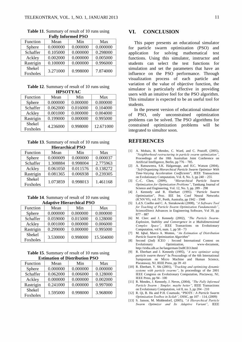
Table 11. Summary of result of 10 runs using
Fully Informed PSO
Function Mean Min Max
Sphere 0.000000 0.000000 0.000000
Schaffer 0.105000 0.000000 0.298000
Ackley 0.002000 0.000000 0.005000
Rastrigin 0.100000 0.000000 0.996000
Shekel
Foxholes 3.271000 0.998000 7.874000
Table 12. Summary of result of 10 runs using
HPSOTYAC
Function Mean Min Max
Sphere 0.000000 0.000000 0.000000
Schaffer 0.062000 0.016000 0.104000
Ackley 0.001000 0.000000 0.004000
Rastrigin 0.199000 0.000000 0.995000
Shekel
Foxholes 4.236000 0.998000 12.671000
Table 13. Summary of result of 10 runs using
Hierarchical PSO
Function Mean Min Max
Sphere 0.000009 0.000000 0.000037
Schaffer 1.308884 0.998004 2.775963
Ackley 0.061050 0.011576 0.138272
Rastrigin 0.081365 0.006938 0.239305
Shekel
Foxholes 1.073859 0.998013 1.461168
Table 14. Summary of result of 10 runs using
Adaptive Hierarchical PSO
Function Mean Min Max
Sphere 0.000000 0.000000 0.000000
Schaffer 0.059000 0.015000 0.128000
Ackley 0.001000 0.000000 0.006000
Rastrigin 0.299000 0.000000 0.995000
Shekel
Foxholes 3.530000 0.998000 15.504000
Table 15. Summary of result of 10 runs using
Estimation of Distribution PSO
Function Mean Min Max
Sphere 0.000000 0.000000 0.000000
Schaffer 0.062000 0.006000 0.128000
Ackley 0.000000 0.000000 0.002000
Rastrigin 0.241000 0.000000 0.997000
Shekel
Foxholes 1.595000 0.998000 3.968000
VI. CONCLUSION
This paper presents an educational simulator
for particle swarm optimization (PSO) and
application for solving mathematical test
functions. Using this simulator, instructor and
students can select the test functions for
simulation and set the parameters that have an
influence on the PSO performance. Through
visualization process of each particle and
variation of the value of objective function, the
simulator is particularly effective in providing
users with an intuitive feel for the PSO algorithm.
This simulator is expected to be an useful tool for
students.
In the present version of educational simulator
of PSO, only unconstrained optimization
problems can be solved. The PSO algorithms for
constrained optimization problems will be
integrated to simultor soon.
REFERENCES [1] A. Mohais, R. Mendes, C. Ward, and C. Postoff, (2005),
“Neighborhood restructuring in particle swarm optimization”,
Proceedings of the 18th Australian Joint Conference on
Artificial Intelligence, Berlin, pp 776 – 785.
[2] A. Ratnaweera, S.K. Halgamuge, and H.C. Watson (2004),
“Self-Organizing Hierarchical Particle Swarm Optimizer With
Time-Varying Acceleration Coefficients”, IEEE Transactions
on Evolutionary Computation, Vol. 8, No. 3, pp 240 – 255
[3] C.-C. Chen, (2009), “Hierarchical Particle Swarm
Optimization for Optimization Problems”, Tamkang Journal of
Science and Engineering, Vol. 12, No. 3, pp. 289 – 298
[4] J. Kennedy and R. Eberhart (1995). “Particle Swarm
Optimization”, Proc. IEE Int. Conf Neural Networks
(ICNN‟95), vol. IV, Perth, Australia, pp 1942 – 1948
[5] L.d.S. Coelho and C. A. Sierakowski (2008), “A Software Tool
for Teaching of Particle Swarm Optimization Fundamentals”,
ScienceDirect Advances in Engineering Software, Vol 39, pp
877 – 887
[6] M. Clerc and J. Kennedy (2002), “The Particle Swarm-
Explosion, Stability and Convergence in a Multidimensional
Complex Space”, IEEE Transactions on Evolutionary
Computation, vol 6, num. 1, pp 58 - 73
[7] M. Iqbal, Marco A. Montes, “An Estimation of Distribution
Particle Swarm Optimization Algorithm”
[8] Second (2nd) ICEO : Second International Contest on
Evolutionary Optimization, www-document,
http://iridia.ulb.ac.be/langerman/2ndICEO.html
[9] R. Eberhart and J. Kennedy (1995), “A new optimizer using
particle swarm theory” In Proceedings of the 6th International
Symposium on Micro Machine and Human Science,
Piscataway, NJ, IEEE Press, pp 39 -43
[10] R. Eberhart, Y. Shi (2001), “Tracking and optimizing dynamic
systems with particle swarms”, In proceedings of the 2001
IEEE Congress on Evolutionary Computation, Pisctaway, NJ,
IEEE Press, pp 94 - 100
[11] R. Mendes, J. Kennedy, J. Neves, (2004), “The Fully Informed
Particle Swarm : Simpler, maybe better”, IEEE Transactions
on Evolutionary Computation, vol 8, no. 3, pp 204 - 210
[12] R. Qi, B. Hu and P.H. Cournede, “PSOTS : A Particle Swarm
Optimization Toolbox in Scilab”, OSSC, pp 107 – 114, (2009)
[13] S. Janson, M. Middendorf, (2005), “A Hierarchical Particle
Swarm Optimizer and Its Adaptive Variant”, IEEE
12 TELEKONTRAN, VOL. 1, NO. 1, JANUARI 2013
Transactions on Systems, Man and Cybernetics, Vol. 35, No 6,
pp 1272 – 1282
[14] W. N. Lee and J. B. Park (2011), “Educational Simulator for
Partilce Swarm Optimization and Economic Dispatch
Applications”, MATLAB – A Ubiquitous Tool for the Practical
Engineer, pp 81 – 110
[15] Y. L.. Zheng, L.H. Ma, L.Y. Zhang, J.X. Qian, (2003)
“Empirical study of particle swarm optimizer with an
increasing inertia weight”, In: Proceedings of the 2003 IEEE
Congress on Evolutionary Computation, Piscataway, NJ, IEEE
Press, pp 221 - 226
[16] Y. Shi, R. Eberhart (1999), “Empirical study of particle swarm
optimization”, In: Proceedings of the 1999 IEEE Congress on
Evolutionary Computation, Piscatawaym, NJ, IEEE Press, pp
1945 - 1950
[17] Birge B. “PSOt – a particle swarm optimization toolbox for use
with Matlab.” Proceedings of the swarm intelligence
symposium Indianapolis, USA, pp 182 – 186, (2003)
[18] Hartmut Pohlheim, “Genetic and Evolutionary Algorithm
Toolbox for Matlab : GEATbx Examples; Examples of
Objective Functions”, (December 2006)
[19] Hartmut Pohlheim, “Genetic and Evolutionary Algorithm
Toolbox for Matlab : GEATbx Introduction; Evolutionary
Algorithms: Overview, Methods and Operators” , (December
2006)
[20] Hartmut Pohlheim, “Genetic and Evolutionary Algorithm
Toolbox for Matlab : GEATbx Tutorial” , (December 2006)
[21] Kenneth Lee, “Particle Swarm Optimization and Social
Interactions Between Agents”, (2008)
[22] J. K. Vis, “Particle Swarm Optimizer for Finding Robust
Optima”, (June 2009)
[23] Juan R. Castro, Oscar Castillo, Luis G. Martinez, “Interval
Type-2 Fuzzy Logic Toolbox”
[24] Marco A. Montes, T. Stutzle, M. Birattari and M. Dorigo, “A
Comparison of Particle Swarm Optimization Algorithms Based
on Run-Length Distributions”
[25] Marco A. Montes, “On the Performance of Particle Swarm
Optimizers”, IRIDIA (2006)
[26] M. Settles, “An Introduction to Particle Swarm Optimization”,
(November 2005)
[27] R. Poli, J. Kennedy and T. Blackwell, “Particle Swarm
Optimization : An Overview”, Swarm Intell, Vol. 1, pp 33 – 57,
(August 2007)
[28] R. C. Eberhart, Y. Shi, “Particle Swarm Optimization:
Developments, Applications and Resources”, IEEE, pp 81 – 86,
(2001)
[29] R. Umarani, V. Selvi, “Particle Swarm Optimization –
Evolution, Overview and Application”, International Journal of
Engineering Science and Technologi, Vol. 2(7), pp 2802 –
2806, (2010)
[30] S. Das, A. Abraham, A. Konar, “Particle Swarm Optimization
and Differential Evolution Algorithms : Technical Analysis,
Application and Hybridization Perspectives”, Studies in
Computational Intelligence, 116, pp 1-38, (2008)
[31] “Simple Optimization Toolbox For Use with Matlab”,
(November 2006)
[32] Ernesto P. Adorio, MVF – Multivariate Test Functions Library
in C for Unconstrained Global Optimization, (2005)
[33] Hartmun Pohlheim, Genetic and Evolutionary Algorithm
Toolbox for Matlab (GEATbx) Examples of Objective
Functions, (2006)
[34] M. Montaz Ali, A Numerical Evaluation of Several Stochastic
Algorithms on Selected Continuous Global Optimization Test
Problem, (2005)
[35] Marcin Molga, Czeslas Smutnicki, Test Function for
Optimization Need, (2005)
[36] Kaj Madsen, Julius Zilinskas, Testing branch-and-bound
methods for global optimization, (2000)
[37] Xin-She Yang, Test Problem in Optimization, in: Engineering
Optimization: An Introduction with Metaheuristic Applications
(Eds Xin-She Yang), John Wiley & Sons. (2010)
[38] A. Georgieva, I. Jordanov, “Global Optimization Based on
Novel Heuristics, Low-Discrepancy Sequences and Genetic
Algorithms”, European Journal of Operational Research, Vol.
196, pp 413 – 422, (2009)
[39] Ali, M., Pant, M. And Abraham, A. “Simplex Differential
Evolution”, Acta Polythechnica Hungarica, Vol. 6, No. 5,
(2009)
[40] Aluffi-Pentini, F., Parisi, V. And Zirilli, F., Global
Optimization and Stochastic Differential Equations. Journal of
Optimization Theory and Application 47, 1-16., (1985)
[41] Benke,K.K. and Skinner, D.R., A Direct Search Algorithm for
Global Optimization of Multivariate Functions. The Autralian
Computer Journal 23, 73 – 85. (1991)
[42] Bohachevsky, M.E., Johnson, M.E. and Stein, M.L.,
Generalized Simulated Annealing for Function Optimization,
Technometrics 28, 209-217., (1986)
[43] Breiman, L. and Cutler, A., A Deterministic Algorithm for
Global Optimization, Mathematical Programming 58, 179 –
199., (1993)
[44] Corana, A., Marchesi, M., Martini, C. and Ridella, S.,
Minimizing Multimodal Functions of Continuous Variables
with the “Simulated Annealing Algorithm”, ACM Transactions
on Mathematical Software, pp 272 – 280, (1987)
[45] Dekkers, A. And Aarts, E., Global Optimization and Simulated
Annealing, Mathematical Programming 50, pp. 367 – 393,
(1991)
[46] Dixon, L. And Szego, G., Toward Global Optimization, North
Holland, New York, (1975)
[47] Dixon, L. and Szego, G., Toward Global Optimization, Vol. 2,
North Holland, New York, (1978)
[48] Griewank, A.O., Generalized Descent for Global Optimization.
Journal of Optimization Theory and Applications 34, 11-39,
(1981)
[49] Himmelblau, D.M., Applied Nonlinear Programming,
McGraw-Hill, New York, (1972)
[50] Ingber, L., Simulated Annealing : Practice Versus Theory,
Jurnal of Mathematical and Computer Modeling, Vol. 18, no
11, pp 29 – 57, (1993)
[51] Jansson, C. And Knuppel, O., A Branch and Bound Algorithm
for Bound Constrained Optimization Problems without
Derivatives. Journal of Global Optimization 7, 297 – 331,
(1995)
[52] K. Muller and L. D. Brown, Location of Saddle Points and
Minimum Energy Paths by a Constrained Simplex Optimization
Procedure, Theoret. Chim. Acta, 53:75-93, (1979)
[53] Kwon, Y.D., Kwon, S.B., and Kim, J.Y., Convergence
Enhanced Genetic Algorithm with Successive Zooming Method
for Solving Continuous Optimization Problems, Computers and
Structures 81, pp. 1715 – 1725, (2003)
[54] Levy, A.V. and Montalvo, A., The Tunneling Algorithm for the
Global Minimization of Functions. Society for Industrial and
Applied Mathematics 6, 15 – 29, (1985)
[55] M. J. Hirsch, P. M. Pardalos, M.G.C.Resende, Speeding Up
Continuous Grasp, AT&T Labs Research Technical Report,
(2006)
[56] Mathworks, Global Optimization Toolbox User’s Guide, 2011
[57] McCormick, G.P., Applied Nonlinear Programming, Theory,
Algorithms and Applications, John Wiley and Sons, New York,
(1982)
[58] Muhlenbein, H., Schomisch, S. and Born, J., The Parallel
Genetic Algorithm s Function Optimizer, Proceedings of the
Fourth International Conference on Genetic Algorithms,
Morgan Kaufman : 271-278, (1991)
[59] Neumaier, A., Global and Local Optimization, www-
document, http://solon.cma.univie.ac.at/~neum/glopt.html,
(2003)
[60] Price, W. L., Global Optimization by Controlled Random
Search, Computer Journal 20, 367 – 370, (1977)
[61] Price, K.V., Private Communication, 836 Owl Circle,
Vacaville, CA 95687, (2002)
[62] Michalewicz, Z., Genetic Algorithms + Data Structures =
Evolution Programs, Springer-Verlag, Berlin/Heidelberg/New
York, (1996)
[63] Rody P. S. Oldenhuis, www-document, (2009)
[64] Salomon, R., Reevaluating Genetic Algorithms Performance
Under Coordinate Rotation of Benchmark Functions,
BioSystems 39(3): 263 – 278, (1995)
[65] Schwefel, H.P., Evolution and Optimum Seeking, John Wiley
and Sons, New York, (1995)

13 TELEKONTRAN, VOL. 1, NO. 1, JANUARI 2013
[66] Storn, R. And Price, K., Differential Evolution : A Simple and
Efficient Heuristic for Global Optimization Over Continuous
Spaces. Journal of Global Optimization 11, 341 – 359, (1997)
[67] Thangaraj, R., Pant, M., Abraham A. And Snasel, V. Modified
Particle Swarm Optimization with Time Varying Velocity
Vector, International Journal of Innovative Computing,
Information and Control, Vol. 8, Num. 1(A), (2012)
[68] Torn, A. And Zilinskas, A., Global Optimization, Lecture
Notes in Computer Science, Vol. 350, Springer-Verlag,
Berlin/Heidelberg/New York, (1989)
[69] W. Wang, T.-M. Hwang, C.Juang, J. Juang, C.-Y. Liu and W.-
W. Lin., Chaotic Behaviors of Bistabe Laser Diodes and Its
Application in Synchronization of Optical Communication,
Japanese Journal of Applied Physics, 40 (10) : 5914-5919,
(2001)
[70] Wolfe, M.A, Numerical Methods for Unconstrained
Optimization, Van Nostrand Reinhold Company, New York,
(1978)
[71] Zabinsky, Z.B. Graesser, D.L., Tuttle, M.E. and Kim, G.I.,
Global Optimization of Composite Laminates using Improving
Hit and Run, In: Floudas C. And Pardalos P. (eds.), pp. 343 –
368. Recent Advances in Global Optimization, Princeton
University Press, (1992)

14 TELEKONTRAN, VOL. 1, NO. 1, JANUARI 2013
Appendix A. A Collection of Benchmark Optimization Test Problems
No Name Source No. Of
Vars.
Upper Bound,
Lower Bound Global Optimum
1. Ackley Function Storn & Price (1997) 1 – N (-32.768, 32.768) 0
2. Alphine Function R. Thangaraj et al. (2012) 1 – N (-10, 10) 0
3. Aluffi-Pentini Function Aluffi-Pentiti et al. (1985) 2 (-10,10) -0.3523
4. Banana Shape Function 2 (-2, 2) -25
5. Beale Function Ernesto P. Adorio (2005) 2 (-4.5, 4.5) 0
6. Becker & Lago Function Price (1997) 2 (-10, 10) 0
7. Bird Function 2 (-20, 20) -106.764536
8. Bohachevsky 1 Function Bohachevsky et al. (1986) 2 (-50, 50) 0
9. Bohachevsky 2 Function Bohachevsky et al. (1986) 2 (-50, 50) 0
10. Booth Function Ernesto P. Adorio (2005) 2 (-10, 10) 0
11. Box and Betts Function Kaj Madsen (2000) 3 (0.9, 1.2); (9,
11.2); (0.9, 1.2) 0
12. Branin RCOS Function Dixon and Szego (1978) 2 (-5, 10); (0, 15) 0.397887357
13. Bukin Function 2 (-20, 20) 0
14. Camel Function 2 (-2, 2) -7.0625
15. 3-Hump Camel Function Dixon and Szego (1975) 2 (-5, 5) 0
16. 6-Hump Camel Function Dixon and Szego (1975) 2 (-5, 5) -1.03162845
17. Carrom Table Function Rody P. S. O. (2009) 2 (-10, 10) -24.1568155
18. Chichinadze Function Rody P. S. O. (2009) 2 (-30, 30) -42.9443870
19. Colville Function Ali, M. et. Al (2009) 4 (0, 10) 0
20. Corana‟s Parabola Function Corana (1987) 4 (-1000, 1000) 0
21. Cosine Mixture Function Breiman and Culter (1993) 1 – N (-1, 1) 0.2 for N = 2 0.4 for N = 4
22. Cross-in-tray Function Rody P. S. O. (2009) 2 (-10, 10) -2.06261187
23. Cross-leg table Function Rody P. S. O. (2009) 2 (-10, 10) -1
24. Crowned Cross Function Rody P. S. O. (2009) 2 (-10, 10) 0.0001
25. Deceptive Functions Marcin Molga (2005) 2 - N (0, 1)
26. Dekkers and Aarts Function Dekkers and Aarts (1991) 2 (-10, 10) -24777
27. Dixon and Price Function 1 – N (-10, 10)
28. Drop Wave Functions Marcin Molga (2005) 2 (-5.12, 5.12) -1
29. Easom‟s Functions Michalewicz (1996) 2 – N (-60, 60) -1
30. Eggholder Function Ernesto P. Adorio (2005) 2 – N (-512, 512) -959.64 for N = 2
31. Epistatic Michalewicz
Function Second ICEO 5, 10 (0, pi) -4.687658 for N = 5
32. Exponential Function Breiman and Culter (1993) 1 – N (-1, 1) 1
33. Giunta Function Rody P. S. O. (2009) 2 (-1, 1) 0,0644704205
34. Goldstein-Price‟s function Dixon and Szego (1978) 2 (-2, 2) 3
35. Griewank „s Function Griewank (1981) 1 – N (-600, 600) 0
36. Gulf Research Problem Himmelblau (1972) 3 (0.1, 100) 0
37. Hartman 3 Problem Dixon and Szego (1978) 3 (0, 1) -3.86278214782
38. Hartman 6 Problem Dixon and Szego (1978) 6 (0,1) -3.32236801141
39. Helical Valley Problem Wolfe (1978) 3 (-10, 10) 0
40. Himmelblau Function Ernesto P. Adorio (2005) 2 (-6, 6) 0
41. Holder Table Function Rody P. S. O. (2009) 2 (-10, 10) -19.2085025678
42. Hosaki Function Benke and Skinner (1991) 2 (0, 6) -2.3458
43. Hyper-ellipsoid function Storn & Price (1997) 1 – N (-5.12, 5.12) 0
44. Kowalik Function Jansson and Knuppel
(1995) 4 (0, 0.42) 0.00030748
45. Kwon Function Kwon (2003) 2 (-1, 1) -16.0917200
46. Langermann‟s Function Marcin Molga (2005) 2 (0, 10) -4.15581
47. Levy and Montalvo 1 Function Levy and Montalvo (1985) 1 – N (-10, 10) 0
48. Levy and Montalvo 2 Function Levy and Montalvo (1985) 1 – N (-10, 10) 0
49. Lyapunov Exponents Wang (2001) 2 (20, 30)
50. Matyas Function Ernesto P. Adorio (2005) 2 (-10, 10) 0
51. McCormik Function McCormik (1982) 2 (-1.5, 4), (-3, 3) -1.9133
52. Meyer and Roth Function Wolfe, 1978 3 (-10, 10) 0.0004
53. Michalewicz‟s Function Second ICEO 2 – N (0, pi) -1.8013 for N = 2 -4.6876 for N = 5
-9.660 for N = 10
54. Miele and Cantrell Function Wolfe, 1978 4 (-1, 1) 0

15 TELEKONTRAN, VOL. 1, NO. 1, JANUARI 2013
55. Modified Langerman Function Second ICEO 5, 10 (0, 10) -0.965
56. Muller-Brown Surface
Function K. Muller, (1979) 2 (-1.5, 1) -146. 699
57. Multi-Gaussian Function Benke & Skinner, (1991) 2 (-2, 2) 1.29695
58. Multimod Function Ernesto P. Adorio (2005) 1 – N (-10, 10) 0
59. Neumaier 2 Function Neumaier (2003) 4 (0, 4) 0
60. Neumaier 3 Function Neumaier (2003) 2 – N (-N^2, N^2) -(N*(N+4)*(N-1))/6
61. Odd Square Function Second ICEO 2 – 20 (-15, 15) -1.143833
62. Paviani Function Kaj Madsen, 2000 10 (2.001, 9.999) -45.77847
63. Peaks Function Mathworks, 2011 2 (-4, 4) -6.55113
64. Penholder Function Rody P. S. O. (2009) 2 (-11, 11) -0.9635348327265
65. Periodic Function Price (1977) 2 (-10, 10) 0.9
66. Perm Function Xin-She Yang (2010) 2 - N (-N, N) 0
67. Perm0 Function Xin-She Yang (2010) 2 - N (-N, N) 0
68. Powell‟s Quadratic Function Wolfe (1978) 4 (-10, 10) 0
69. Price‟s Transistor Modelling
Function Price (1977) 9 (-10, 10) 0
70. Quartic Function Ali, M. et. Al (2009) 2 – N (-1.28, 1.28) Random
71. Rastrigin‟s Function Torn and Zilinskas (1989) 1 – N (-5.12, 5.12) 0
72. Rosenbrock‟s Function Schwefel (1995) 2 – N (-2.048, 2.048) 0
73. Rotated Hyper-Ellipsoid
Function Marcin Molga (2005) 1 – N (-65.536, 65.536) 0
74. Salomon Function Salomon (1995) 2 – N (-100, 100) 0
75. Sawtoothxy Function Mathworks, 2011 2 (-20, 20) 0
76. Schaffer 1 Function Michalewicz (1996) 2 – N (-100, 100) 0
77. Schaffer 2 Function Michalewicz (1996) 2 – N (-100, 100) 0
78. Schwefel‟s Function Muhlenbein (1991) 1 – N (-500, 500) -418.9829N
79. Shekel 5 Function Dixon and Szego (1978) 4 (0, 10) -10.1531996790582
80. Shekel 7 Function Dixon and Szego (1978) 4 (0, 10) -10.4029405668187
81. Shekel 10 Function Dixon and Szego (1978) 4 (0, 10) -10.5364098166920
82. Shekel‟s Foxholes Marcin Molga (2005) 2 (-65.536, 65.536) 0.998004
83. Shekel‟s Foxholes Function 5d Dixon and Szego (1978) 5, 10 (0, 10) -10.5046, fot N = 5
84. Shubert‟s Function Levy and Montalvo (1985) 2 – N (-10, 10) -186.7309, for N = 2
85. Shubert‟s Function 2 R. Thangaraj et al. (2012) 2 – N (-10, 10) -24.062499
86. Sinusoidal Function Zabinsky (1992) 2 – N (0, 180) -(A+1), default A =
2.5
87. Sphere Function Storn & Price (1997) 1 – N (-5.12, 5.12) 0
88. Step Function R. Thangaraj et al. (2012) 1 – N (-1, 1) 0
89. Sum of Different Power
Functions Marcin Molga (2005) 1 – N (-1, 1) 0
90. Storn‟s Tchebychev Function Price (2002) 9 (-128, 128) 0
91. Testtube holder function Rody P. S. O. (2009) 2 (-10, 10) -10.872299901558
92. Trefethen4 Function Ernesto P. Adorio (2005) 2 (-6.5, 6.5); (-4.5,
4.5) -3.30686865
93. Trid Function M.J.Hirsch (2006) 2 – N (-N^2, N^2) -50 for N = 6
-210 for N = 10
94. Tripod Function Ali, M. et. Al (2009) 2 (-100, 100) 0
95. Whitley Function A. Georgieva (2009) 2 – N (-100, 100) 0
96. Wood Function Wolfe (1978) 4 (-10, 10) 0
97. Xin-She Yang‟s Function 1 Xin-She Yang (2010) 1 – N (-2pi, 2pi) 0
98. Xin-She Yang‟s Function 2 Xin-She Yang (2010) 1 – N (-10, 10) -0.6065
99. Xin-She Yang‟s Function 3 Xin-She Yang (2010) 2 – N (-20, 20) -1 for beta = 15
100. Xin-She Yang‟s Function 4 Xin-She Yang (2010) 1 – N (-10, 10) -1
101. Xin-She Yang‟s Function 5 Xin-She Yang (2010) 2 (0, 10) Random
102. Zakharov Function Xin-She Yang (2010) 2 – N (-10, 10) 0
103. Zettl Function Rody P. S. O. (2009) 2 (-10, 10) -0.0037912372204